1
The Cache Visualisation Tool
Eric van der Deijl
May 1995
Gerco Kanbier
Contents
1 Introduction
2 Cache Theory
2.1
2.2
2.3
2.4
2.5
2.6
Introduction to caches :
Set Associativity : : : :
Cache line identication
Replacement policies :
Write Policies : : : : :
Problems with caches :
:
:
:
:
:
:
:
:
:
:
:
:
:
:
:
:
:
:
:
:
:
:
:
:
:
:
:
:
:
:
:
:
:
:
:
:
:
:
:
:
:
:
:
:
:
:
:
:
:
:
:
:
:
:
:
:
:
:
:
:
:
:
:
:
:
:
:
:
:
:
:
:
:
:
:
:
:
:
:
:
:
:
:
:
:
:
:
:
:
:
:
:
:
:
:
:
:
:
:
:
:
:
:
:
:
:
:
:
:
:
:
:
:
:
:
:
:
:
:
:
:
:
:
:
:
:
:
:
:
:
:
:
:
:
:
:
:
:
:
:
:
:
:
:
:
:
:
:
:
:
:
:
:
:
:
:
:
:
:
:
:
:
:
:
:
:
:
:
:
:
:
:
:
:
:
:
:
:
:
:
:
:
:
:
:
:
:
:
:
:
:
:
3.1 The global structure : : : : : : : : : :
3.2 The Screen : : : : : : : : : : : : : : :
3.2.1 The Cache Area : : : : : : : :
3.2.2 The Statistics Area : : : : : :
3.3 Controlling the CVT : : : : : : : : : :
3.3.1 Button "> j" One Step : : : : :
3.3.2 Button ">" Run : : : : : : : :
3.3.3 Button ">>" Fast Forward : :
3.3.4 Button "<<" Rewind : : : : :
3.3.5 Button "jj" Pause : : : : : : :
3.3.6 Button "#" Abort : : : : : : :
3.3.7 Button "Flush" : : : : : : : : :
3.3.8 Button "Arr/Ref" : : : : : : :
3.3.9 Button "Save As" : : : : : : : :
3.3.10 Button "Save" : : : : : : : : :
3.3.11 Button "Load" : : : : : : : : :
3.3.12 Button "ToggleEI" : : : : : : :
3.3.13 Speed : : : : : : : : : : : : : :
3.4 Menu-Option Tool : : : : : : : : : : :
3.4.1 Sub-Option About Tool : : : :
3.4.2 Sub-Option Set Fast Forward :
3.4.3 Sub-Option Set Rewind : : : :
3.4.4 Sub-Option Static Parameters
3.4.5 Sub-Option Quit : : : : : : : :
3.5 Menu-Option File : : : : : : : : : : :
3.5.1 Sub-Option Load Program : :
3.5.2 Sub-Option Show CVT code : :
3.5.3 Sub-Option Show Original : : :
3.5.4 Sub-Option Load Trace : : : :
3.5.5 Sub-Option Load Source-Trace
3.6 Menu-Option Colors : : : : : : : : : :
:
:
:
:
:
:
:
:
:
:
:
:
:
:
:
:
:
:
:
:
:
:
:
:
:
:
:
:
:
:
:
:
:
:
:
:
:
:
:
:
:
:
:
:
:
:
:
:
:
:
:
:
:
:
:
:
:
:
:
:
:
:
:
:
:
:
:
:
:
:
:
:
:
:
:
:
:
:
:
:
:
:
:
:
:
:
:
:
:
:
:
:
:
:
:
:
:
:
:
:
:
:
:
:
:
:
:
:
:
:
:
:
:
:
:
:
:
:
:
:
:
:
:
:
:
:
:
:
:
:
:
:
:
:
:
:
:
:
:
:
:
:
:
:
:
:
:
:
:
:
:
:
:
:
:
:
:
:
:
:
:
:
:
:
:
:
:
:
:
:
:
:
:
:
:
:
:
:
:
:
:
:
:
:
:
:
:
:
:
:
:
:
:
:
:
:
:
:
:
:
:
:
:
:
:
:
:
:
:
:
:
:
:
:
:
:
:
:
:
:
:
:
:
:
:
:
:
:
:
:
:
:
:
:
:
:
:
:
:
:
:
:
:
:
:
:
:
:
:
:
:
:
:
:
:
:
:
:
:
:
:
:
:
:
:
:
:
:
:
:
:
:
:
:
:
:
:
:
:
:
:
:
:
:
:
:
:
:
:
:
:
:
:
:
:
:
:
:
:
:
:
:
:
:
:
:
:
:
:
:
:
:
:
:
:
:
:
:
:
:
:
:
:
:
:
:
:
:
:
:
:
:
:
:
:
:
:
:
:
:
:
:
:
:
:
:
:
:
:
:
:
:
:
:
:
:
:
:
:
:
:
:
:
:
:
:
:
:
:
:
:
:
:
:
:
:
:
:
:
:
:
:
:
:
:
:
:
:
:
:
:
:
:
:
:
:
:
:
:
:
:
:
:
:
:
:
:
:
:
:
:
:
:
:
:
:
:
:
:
:
:
:
:
:
:
:
:
:
:
:
:
:
:
:
:
:
:
:
:
:
:
:
:
:
:
:
:
:
:
:
:
:
:
:
:
:
:
:
:
:
:
:
:
:
:
:
:
:
:
:
:
:
:
:
:
:
:
:
:
:
:
:
:
:
:
:
:
:
:
:
:
:
:
:
:
:
:
:
:
:
:
:
:
:
:
:
:
:
:
:
:
:
:
:
:
:
:
:
:
:
:
:
:
:
:
:
:
:
:
:
:
:
:
:
:
:
:
:
:
:
:
:
:
:
:
:
:
:
:
:
:
:
:
:
:
:
:
:
:
:
:
:
:
:
:
:
:
:
:
:
:
:
:
:
:
:
:
:
:
:
:
:
:
:
:
:
:
:
:
:
:
:
:
:
:
:
:
:
:
:
:
:
:
:
:
:
:
:
:
:
:
:
:
:
:
:
:
:
:
:
:
:
:
:
:
:
:
:
:
:
:
:
:
:
:
:
:
:
:
:
:
:
:
:
:
:
:
:
:
:
:
:
:
:
:
:
:
:
:
:
:
:
:
:
:
:
:
:
:
:
:
:
:
:
:
:
:
:
:
:
:
:
:
:
:
:
:
:
:
:
:
:
:
:
:
:
:
:
:
:
:
:
:
:
:
:
:
:
:
:
:
:
:
:
:
:
:
:
:
:
:
:
:
:
:
:
:
:
:
:
:
:
:
:
:
:
:
:
:
:
:
:
:
:
:
:
:
:
:
:
:
:
:
:
:
:
:
:
:
:
:
:
:
:
:
:
:
:
:
:
:
:
:
:
:
:
:
:
:
:
:
:
:
:
:
:
:
:
:
:
:
:
:
:
:
:
:
:
:
:
:
:
:
:
:
:
:
:
:
:
:
:
:
:
:
:
:
:
:
:
:
:
:
:
:
:
:
:
:
:
:
:
:
:
:
:
:
:
:
:
:
:
:
:
:
:
:
:
:
:
:
:
:
:
:
:
:
:
:
:
:
:
:
:
:
:
:
:
:
:
:
:
:
:
:
:
:
:
:
:
:
:
:
:
:
:
:
:
:
:
:
:
:
:
:
:
:
:
:
:
:
:
:
:
:
:
:
:
:
:
:
:
:
:
:
:
:
:
:
:
:
:
:
:
:
:
:
:
:
:
:
:
:
:
:
:
:
:
:
:
:
:
:
:
:
:
:
:
:
:
:
:
:
:
:
:
:
:
:
:
:
3 CVT Description
:
:
:
:
:
:
:
:
:
:
:
:
:
:
:
:
:
:
:
:
:
:
:
:
:
:
:
:
:
:
:
:
:
:
:
:
:
:
:
:
:
:
1
4
6
6
7
7
8
8
9
10
10
12
13
13
16
17
18
19
19
20
20
20
20
20
21
21
21
21
22
23
23
23
24
25
25
25
26
26
27
28
28
3.6.1
3.6.2
3.6.3
3.6.4
Sub-Option Show/Change Array Colors
Sub-Option Show/Change RefID Colors
Sub-Option Show PC Colors : : : : : :
Sub-Option Color Mode : : : : : : : : :
3.7 Menu-Option Breakpoints : : : : : : : : : : : :
3.7.1 Sub-Option Add Cache Breakpoint : : :
3.7.2 Sub-Option Timer Breakpoint : : : : : :
3.7.3 Sub-Option Add Loop value Breakpoint
3.7.4 Sub-Option Add Statement Breakpoint :
3.7.5 Sub-Option Add PC Breakpoint : : : :
3.7.6 Sub-Option Show List of Breakpoints :
3.8 Menu-Option Parameters : : : : : : : : : : : :
::::::::::
::::::::::
::::::::::
::::::::::
::::::::::
::::::::::
::::::::::
::::::::::
::::::::::
::::::::::
::::::::::
::::::::::
3.8.1 Architecture : : : : : : : : : : : : : : : : : : : : : : : : :
3.8.2 Write policy : : : : : : : : : : : : : : : : : : : : : : : : : :
3.8.3 Allocate policy : : : : : : : : : : : : : : : : : : : : : : : :
3.8.4 Replacement policy : : : : : : : : : : : : : : : : : : : : : :
3.9 Menu-Option Others : : : : : : : : : : : : : : : : : : : : : : : : :
3.9.1 Refresh screen : : : : : : : : : : : : : : : : : : : : : : : :
3.9.2 Grid Mode : : : : : : : : : : : : : : : : : : : : : : : : : :
3.9.3 Swap Page : : : : : : : : : : : : : : : : : : : : : : : : : :
3.9.4 Sub-Option Messages : : : : : : : : : : : : : : : : : : : :
3.9.5 Sub-Option Extra Info : : : : : : : : : : : : : : : : : : :
3.10 Making the Input : : : : : : : : : : : : : : : : : : : : : : : : : : :
3.10.1 Program : : : : : : : : : : : : : : : : : : : : : : : : : : :
3.10.2 Traces : : : : : : : : : : : : : : : : : : : : : : : : : : : :
3.10.3 Source-Traces : : : : : : : : : : : : : : : : : : : : : : : : :
3.11 Further Tuning : : : : : : : : : : : : : : : : : : : : : : : : : : : :
3.11.1 The Simulator : : : : : : : : : : : : : : : : : : : : : : : :
3.11.2 Using and changing CVT's data structures and variables
:
:
:
:
:
:
:
:
:
:
:
:
:
:
:
:
:
:
:
:
:
:
:
:
:
:
:
:
:
:
:
:
:
:
:
:
:
:
:
:
:
:
:
:
:
:
:
:
:
:
:
:
:
:
:
:
:
:
:
:
:
:
:
:
:
:
:
:
:
:
:
:
:
:
:
:
:
:
:
:
:
:
:
:
:
:
:
:
:
:
:
:
:
:
:
:
:
:
:
:
:
:
:
:
:
:
:
:
:
:
:
:
:
:
:
:
:
:
:
:
:
:
:
:
:
:
:
:
:
:
:
:
:
:
:
:
:
:
:
:
:
:
:
:
:
:
:
:
:
:
:
:
:
:
:
:
:
:
:
:
:
:
:
:
:
:
:
:
:
:
:
:
:
:
Introduction : : : : : : : : : : : : : : : : : : : : : : : : : : : : : : : : : : :
Cache Interferences : : : : : : : : : : : : : : : : : : : : : : : : : : : : : :
Blocking : : : : : : : : : : : : : : : : : : : : : : : : : : : : : : : : : : : :
Nonsingular Loop Transformations : : : : : : : : : : : : : : : : : : : : : :
4.4.1 Some theory : : : : : : : : : : : : : : : : : : : : : : : : : : : : : :
4.4.2 Unimodular transformations of double loops : : : : : : : : : : : : :
4.4.3 Optimizing data locality through unimodular loop transformations
4.4.4 Nonsingular loop transformations : : : : : : : : : : : : : : : : : : :
4.5 Software Prefetching : : : : : : : : : : : : : : : : : : : : : : : : : : : : : :
4.6 Sparse codes : : : : : : : : : : : : : : : : : : : : : : : : : : : : : : : : : :
:
:
:
:
:
:
4 Using the CVT for Software Optimizations
4.1
4.2
4.3
4.4
5 Using the CVT for Hardware Optimizations
5.1 Introduction : : : : : : : : : : : :
5.2 Terminology : : : : : : : : : : : :
5.3 Memory Hierarchy Evaluation :
5.3.1 Cache Parameters : : : :
5.4 Caches : : : : : : : : : : : : : : :
5.5 Replacement policy : : : : : : : :
5.6 Write policy : : : : : : : : : : : :
5.7 Opportunities of the CVT : : : :
5.7.1 How can we do research?
5.7.2 Victim cache : : : : : : :
5.8 Test results : : : : : : : : : : : :
:
:
:
:
:
:
:
:
:
:
:
:
:
:
:
:
:
:
:
:
:
:
:
:
:
:
:
:
:
:
:
:
:
:
:
:
:
:
:
:
:
:
:
:
:
:
:
:
:
:
:
:
:
:
:
:
:
:
:
:
:
:
:
:
:
:
:
:
:
:
:
:
:
:
:
:
:
2
:
:
:
:
:
:
:
:
:
:
:
:
:
:
:
:
:
:
:
:
:
:
:
:
:
:
:
:
:
:
:
:
:
:
:
:
:
:
:
:
:
:
:
:
:
:
:
:
:
:
:
:
:
:
:
:
:
:
:
:
:
:
:
:
:
:
:
:
:
:
:
:
:
:
:
:
:
:
:
:
:
:
:
:
:
:
:
:
:
:
:
:
:
:
:
:
:
:
:
:
:
:
:
:
:
:
:
:
:
:
:
:
:
:
:
:
:
:
:
:
:
:
:
:
:
:
:
:
:
:
:
:
:
:
:
:
:
:
:
:
:
:
:
:
:
:
:
:
:
:
:
:
:
:
:
:
:
:
:
:
:
:
:
:
:
:
:
:
:
:
:
:
:
:
:
:
:
:
:
:
:
:
:
:
:
:
:
:
:
:
:
:
:
:
:
:
:
:
:
:
:
:
:
:
:
:
:
:
:
:
:
:
:
:
:
:
:
:
:
:
:
:
:
:
:
:
:
:
:
:
:
:
:
:
:
:
:
:
:
:
:
:
:
:
:
:
:
:
:
:
:
:
:
:
:
:
:
:
:
:
:
:
:
:
:
:
:
:
:
:
:
:
:
:
:
:
:
:
:
:
:
:
:
:
:
:
:
:
:
:
:
:
:
:
:
:
:
:
:
:
:
:
:
:
:
:
:
:
:
:
:
:
:
:
:
:
:
:
:
:
:
:
:
:
:
:
:
:
:
:
:
:
:
:
:
:
:
:
:
:
:
:
:
:
:
:
:
:
:
:
:
:
:
:
:
:
:
:
:
:
:
:
:
:
:
:
:
:
:
:
:
:
:
:
:
:
:
:
:
:
:
:
:
:
:
:
:
:
:
:
:
:
:
:
:
:
:
:
:
:
:
:
:
:
:
:
:
:
:
:
:
:
:
:
:
:
:
:
:
:
:
:
:
:
:
:
:
:
:
:
:
:
:
:
:
:
:
:
:
:
:
:
:
:
:
:
:
:
:
:
:
:
:
:
:
:
:
:
:
:
:
:
:
:
:
:
:
:
:
:
:
:
:
::
::
::
:
:
:
:
:
:
:
:
:
:
:
:
:
:
:
:
:
:
:
:
:
:
:
:
:
:
:
:
:
:
:
:
:
:
:
:
:
:
:
:
:
:
:
:
:
:
:
:
:
:
:
:
:
:
:
:
:
:
:
:
:
:
:
:
:
:
:
:
:
:
:
:
:
:
:
:
:
:
:
:
:
:
:
:
:
:
:
:
:
:
:
:
:
:
:
:
:
:
:
:
:
:
:
:
:
:
:
:
:
:
:
:
:
:
:
:
:
:
:
:
:
:
:
:
:
:
:
:
:
:
:
:
:
:
:
:
:
:
:
:
:
:
:
:
:
:
:
:
:
:
:
:
:
:
:
:
:
:
:
:
:
:
:
:
:
:
:
:
:
:
:
:
:
:
:
:
:
:
:
:
:
:
:
:
:
:
:
:
:
:
:
:
:
:
:
:
:
:
:
:
:
:
:
:
:
:
:
:
:
:
:
29
32
33
34
34
35
35
36
36
37
37
38
39
40
41
41
41
42
42
42
42
44
45
45
48
48
49
49
51
53
53
54
57
60
61
62
63
65
66
68
71
71
71
71
72
73
73
74
74
75
76
77
5.8.1 Cache size and Set associativity : : : : : : : : : : : : : : : : : : : : : : : : : : : : : : : 77
5.8.2 Cacheline size and Set Associativity : : : : : : : : : : : : : : : : : : : : : : : : : : : : 80
6 Conclusions
A CVT Programs
82
84
B Trace Makers
87
A.1 CVT Code for FLO52 : : : : : : : : : : : : : : : : : : : : : : : : : : : : : : : : : : : : : : : : 84
A.2 CVT code for Blocked Matrix x Matrix : : : : : : : : : : : : : : : : : : : : : : : : : : : : : : 85
A.3 CVT code for SOR : : : : : : : : : : : : : : : : : : : : : : : : : : : : : : : : : : : : : : : : : 86
B.1 Making a trace for software prefetched matrix matrix multiply : : : : : : : : : : : : : : : : : 87
B.2 Making a trace for Sparse Matrix Vector multiply : : : : : : : : : : : : : : : : : : : : : : : : 87
3
Chapter 1
Introduction
This tool is a cache simulator especially developed in order to gain insight into unpredictable cache phenomena which cause a trementous performance slow down on high performance super- computers. Other
previous simulators could only unveil bad performance by indicaters like performance, miss- and hit- ratio.
This simulator can not only show global gures about the performance of a program, but also visualize the
bottle- neck and thus deal with the roots of this problem. The scien- tist is now able to deal with complex
reference patterns which are hard to understand without visualization. With this tool, research can be done
to all kind of programs on all kind of cache hierarchies.
The CVT supports two kind of software; traces and programs. Traces are made by the user; a suspicious
code can be transla- ted into a trace-le where program counter, base address and a read or a write are
stored. Simulation gives an overall view of performance of this particular code. Bottle-necks are visualized
by the statistics, where program counters with a high miss-ratio indicate a bad performance. Often, when
you look in the original program of this trace, this program counter is often used in nested DO-loops. These
structures are highly sensitive to interferences and therefor need a closer look. The user can translate a
suspicious nested DO-loop from the orignal program to the CVT-program format. These programs compiled
by the CVT contain only nested DO-loops. These loops can do a lot of iterations and some data might be
used multip- le times. This opportunity of reuse must be exploited by the cache in order the improve the
performance. Though, instead of reuse the data, it can also be bumped out of cache before it is reused. Now
we're forced to get the data from memory instead of cache, which is a high price we have to pay because we
don't exploit the cache which is developed to improve the performance. This miss-penalty is high because
of the enormous development in cpu-speed and relatively slow memory. Misses caused by cross-, self- and
capacity-interferences must there- for be avoided!
Numerical codes are typical examples where nested-loops and arrays are often used and thus can severely
suer from cross- and self-intereferences. Because of these phenomena, the potential capacity of some
supercomputers lacks with the nal performance, which is crucial for some programs. This tool can be used
to learn about the basic cache behaviour as well for scientic research to unpredictable cache phenomena
in all kind of dierent hard- and software environments. Next to the software support, the CVT supports
dierent hardware environments. New developments can be tested on this tool. The only drawback in this
tool is that the visualization of only one level in a hierarchy is possible at a time. The user will need to
slightly change the simulator and do the simulation for another level in this hierarchy. But in fact the user
can simulate any architecture.
This CVT is a complete tool and can be used for developping new soft- and/or hardware solutions by
visualizing the cache behaviour cristal clear and makes the cache behaviour more predictable and understandable. This is an improvement to previous simulators because only global gures implied a worse performance,
where there was no understanding about the cause of the performance slow-down. Now there is a possiblity
to see the problems we'll deal with and solution can be thought of (which can also be tested, of course)
The next section is a theoretical chapter about caches, where locality is discussed as well as the problems
arising in cache followed by cache policies and set-associativity caches. Chap- ter three is written as a
user-manual. Every possibility in the CVT is thoroughly discussed and an additional picture will clearify
the text. Chapter four discusses the known software techniques to improve the performance and shows the
4
user how to use the tool in order to detect cache phenomena. Chapter ve will test a few known hardware
optimazations and compare several hardware hierarchies. Finally chapter six will give our conclusions about
this subject.
5
Chapter 2
Cache Theory
This chapter presents a general introduction to caches, it can be skipped by users already familiar with
caches and their problems. In the rest of the report, the here discussed terms will be expected to be known
to the readers.
2.1 Introduction to caches
DOI=1,100
DOJ=1,10
A[J] = B[I] c
ENDDO
ENDDO
Figure 2.1: Example program that exhibits temporal and spatial locality.
Cache is the name that has been chosen to represent the level(s) of a memory hierarchy between the CPU
and the main memory. It is faster (but more expensive and smaller) than the main memory and is used to
speed up the memory hierarchy, which is the main bottleneck in high performance computers.
Caches were invented as a result of technology (which made that faster memory designs are more expensive, one of the reasons that caches are smaller than main memories) and of the principle of locality, which
knows two dimensions :
Temporal Locality If an item is referenced, it will tend to be referenced again soon, an example program
is shown in gure 2.1. In this example there is temporal locality through the ten times that the same
element of array B is referenced continuous in time.
Spatial Locality If an item is referenced, nearby items tend to be referenced soon. In the in gure 2.1
shown program, it is obvious that the consecutive elements of array A are providing the loop spatial
locality. Note that if the cache is large enough to hold at least 11 elements there is also temporal
locality for all the elements of array A.
It is important to note that the cache lines form a subset of the data that is present in the main memory.
For larger memory hierarchies (with more layers of caches) this also holds, every byte found on one level is
also present in all levels below (look at gure 2.2).
Success or failure of an access to the cache is designated as a hit or a miss : a hit means that some
requested datum is found in the cache, a miss means that some requested datum is not present in the cache
and needs to be transferred from main memory. The hit ratio is the fraction of memory accesses found in
the cache (there is also the miss ratio, which is 1 - hit ratio).
6
CPU
Cache
Main Memory
Figure 2.2: A memory hierarchy : every byte found on one level is present in all levels below.
There are four important issues associated with caches, cache line placement (discussed in section 2.2),
cache line identication (discussed in section 2.3), cache line replacement (discussed in section 2.4) and the
write policies (discussed in section 2.5). Though caches are an improvement of the memory structure, there
are some problems concerned with caches, which are discussed in section 2.6.
2.2 Set Associativity
If a cache line can be placed in a restricted set of places in cache, the cache is set to be set associative,
where the set is a group of places in cache. A cache line is rst mapped onto a set and then it can be
placed anywhere within the set. If there are n cache lines in a set, the cache placement is called n-way set
associative. When a cache line can appear in only one place in the cache (it is 1-way set associative), the
cache is called to be direct mapped. Another special case is when a cache line can be placed anywhere in the
cache (it is m-way set associative, where m is the number of entries the cache has), in this case, the cache is
called fully associative.
2.3 Cache line identication
The address of a datum is used to probe the cache for the desired cache line. An address is built from a Tag,
Index and block oset, where the Index provides the set in which the requested data must be and the block
oset the oset within the cache line to nd the requested datum. The procedure is to rst check all the
tags of the elements of a set (that is provided by the index part of an address) with the tag that is provided
by the address, which is done in parallel. If one of the elements produced a hit, the data with the oset,
which is provided by the address, is send to the CPU.
In gure 2.3 an example is provided. The cache as drawn in the gure is a cache of 64 elements, a cache
line size of 4 elements and a set associativity of 4 (4-way set associative). The address of the to be referenced
data is 333 (in bit notation 0000000101001101) and it is divided in a Tag, which are the rst 12 bits and has
a value of 44 (bit notation 000000010100), an Index which are the 2 bits after the Tag and has a value of 3
(bit notation 11) and a Block Oset which are the last two bits and has a value of 1 (bit notation 1). The
set in which the to be found data has to be (if it is present) is the third, as is indicated by the Index value
(Check : Block Address MOD # Sets = 83 MOD 4 = 3, where the Block Address is the original address
modulo the number of elements in a cache line (333 MOD 4 = 83). The four blocks in the third set are now
checked in parallel for the tag 44, in the fourth cache line of the set, the tag equation holds and in this cache
line the second element is taken because the block oset (from the original address) is 2. This element is
send to the CPU, it was a hit in cache.
7
Index
Tag
Block
offset
Tags
44
Data
Set 0
Set 1
Set 3
Set 2
Figure 2.3: Cache line identication.
2.4 Replacement policies
The large number of entries of the main memory and the smaller number in cache, make that some entries
in main memory map to the same cache line in cache. This implies that on a miss, there has to be a victim
cache line selected that is swapped out. For direct mapped caches this is no problem, the cache line on which
the entry is mapped is the only one the new entries can come. So, write the old cache line back to main
memory (if necessary) and get the new cache line from main memory into cache. When set associativity
comes into play however, the number of places a cache line can come is larger than one and, if all of the cache
lines are lled, there has to be found a victim cache line which contents are swapped out. This choosing of
a victim cache, asks for a replacement policy.
There are three primary placement policies (which are also implemented in the CVT) :
FIFO The rst-in-rst-out strategy will replace the cache line that was swapped in the longest time
ago.
LRU The Least Recently Used strategy will bump out the cache line that has been used the longest
period ago, this means it has not been used for the longest time.
Random The Random strategy picks, what's in a name, a cache line from the set at random.
2.5 Write Policies
Though reads dominate cache accesses, writes can not be neglected in optimizing cache performance. The
easy case for reads, where the block can be read and the tag is read and compared at the same time, does
not hold for writes. Since the processor species the size of a write, only that portion of a cache line can be
changed, which indicates a read/modify/write sequence. Another problem is that the modifying of a block
8
can not begin until the tag is checked to see if it is a hit. Because this tag checking can not occur in parallel,
writes usually take up more time than reads.
There are two basic policies when writing to cache, which are also implemented in the CVT :
Write through The information is written to both the cache and the main memory.
Write back The information is written only to the cache. The modied cache line is written to main
memory only when it is replaced. The cache line can either be clean, this means there were no
modications made, or dirty, which states that the cache line has been modied. When write back is
implemented, usually there is a dirty bit associated with each cache line. When a cache line is replaced
the cache line is written in main memory only when the cache line is dirty.
There are both advantages to write back and to write through. Write through has the advantages that
read misses don't result in writes to main memory, it is easier to implement and the main memory has the
most current copy of the data. Write back on the other hand has the advantages that writes occur at the
speed of the cache, multiple writes within one block require only one write to main memory and most writes
don't need memory trac, which indicates a less memory band-with.
The just mentioned policies work on the cache line that already contains the correct data, but there has
also to be a policy when the data is not available, a write miss. There are two policies on a write miss, they
are also implemented in the CVT :
Allocate on write The cache line is loaded into the cache, followed by a 'normal' write-hit action as
mentioned in the write policies above.
No allocate on write The cache line is modied in the main memory and not loaded into cache.
While both the allocate policies could be used with either of the write policies, generally the write back
caches use allocate on write (hoping that subsequent writes will be captured by the cache) and write through
caches often use no allocate on write (subsequent writes to the cache line will still have to go to the main
memory).
2.6 Problems with caches
Though caches are a big improvement over older memory hierarchies with no caches, caches induce certain
phenomena, problems that are quite hard to understand and one of the reasons this report (and indeed even
the CVT) exists. The source of trouble is the cache miss, there are three kinds of cache misses :
Compulsory Misses The rst access to a certain cache line is not in cache. They are also called cold
start misses, the cache has to warm up (i.e. ll up) rst, before cache lines can be present in the cache.
Capacity Misses If the cache can not contain all the blocks needed during execution of a program,
capacity misses will occur due to cache lines being discarded and later on retrieved.
Conict Misses A cache line is discarded and later on retrieved if too many cache lines map to the
same set. Conict misses are produced by either self-interference, which means that an array interferes
with itself, or cross-interference which means that an array interferes with another array.
The compulsory misses can be reduced by larger cache lines, but this can increase the number of conict
misses. The capacity misses can be reduced by larger memory chips. The conict misses can be avoided
by getting a fully associative cache, but this is very expensive. Another option is to understand why these
conict misses occur, what arrays are conicting and why they are conicting the way they do. From normal
code this is very hard to understand, but the CVT can be of help here by visualizing the phenomena in
cache.
9
Chapter 3
CVT Description
This chapter will describe the CVT by rst going through the global structure of the Cache Visualization
Tool, then all the options the CVT provides are discussed by going through the menu-options and the realtime possibilities. The last part of this chapter describes how to make programs or traces and how to further
tune the CVT for the users needs (e.g. plugging in her own simulator).
3.1 The global structure
The Cache Visualization Tool (CVT) is built from several source les for modularity. The ".c" les contain
the actual c-codes, the ".h" les contain the functions from the corresponding ".c" le that can be called
from other ".c" les. The le "typedef.h" contains all the global variables and data structures used in the
CVT. The "Makele" associated with the CVT, will set out the route for the make program that compiles
the CVT. The following les are associated with the CVT :
ALLStat.c This le contains functions that aect all statistics. It is 18362 bytes large.
ARStat.c This le contains the functions related to the array- reference statistics. It is a le of 27854
bytes.
ARcolor.c In this le the functions are implemented which are related to coloring by Array Reference
(Showing them on screen/changing them). It is 18461 bytes large.
BRPcallback.c This le contains all the functions concerning breakpoints (entering them, showing them
on screen, enabling/deleting). This le is 50639 bytes large.
CAStat.c (not yet completely done) This le will contains all the functions related to the cache statistics,
24411 bytes large.
Info.c In this le the function related to the extra info that is situated at the right hand side of the
screen, are implemented. The le is 20608 bytes large.
PCStat.c It contains the les related to the program counter/trace statistics. It is 25025 bytes.
PCcolors.c This les contains the function related to the coloring and showing of the Program Counters,
as used with traces, the le is 14978 bytes large.
addColor.c This le contains the functions to add an additional color, it is 11791 bytes large.
addLoopBRP.c To add a loop value breakpoint to the CVT. Size is 9879 bytes.
arraref.c This le contains the functions to keep up with new array references. It is only 5446 bytes
large.
10
cache.c The main le of the CVT, it sets up the global variables and installs all the other routines, it
is only 9641 bytes large.
callback.c In Motif all mouse clicks are handled with call-backs, this le contains the functions that are
called (though there are call-back functions in other les, if that seemed more appropriate). The le
is 86742 bytes large.
checkColor.c In this le the colors of program counters are checked for some reason. Size is 5329 bytes.
checkLoopBRP.c Every state of the DO-loops must be checked whether a loop value breakpoint is true.
This le is 5341 bytes big.
checker.c This le is used to check all boundaries used in the simulation, like DO-loop boundaries.
This le is 14403 bytes large.
cleanup.c This CVT-le is used to clean up all the used structures when we just have aborted the
simulation. Size is 16049 bytes.
colors.c This le contains all the routines related to array coloring (showing the colors, adding additional
colors, changing/selecting/deleting colors). This le is 48398 bytes large.
common.c All functions related to the environment and for common use are stated in this le of 23182
bytes.
cpu.c The cpu will generate memory references from a CVT program every time it is called. This le
is only 14862 bytes large.
graphics.c The graphics is based on Motif1.2 and all graphical stu is described in this le of 1876
bytes.
initializer.c All data-structures concerning a program are initialized in this le. Size is 18514 bytes.
interpreter.c The interpreter reads a program and checks for syntax errors. The le is 44488 bytes
large.
looptrac.c This le contains the functions to run a loop trace (either one-step/ fast-forward/normal
run), it also loads a trace. Size is 22215 bytes.
param.c This le contains the functions for saving and loading the static parameters of the CVT
environment. Plus it contains the functions to allow rewinding of programs, traces and loop traces.
This le is 70794 bytes large.
program.c This le contains the functions to run a program (either one-step/ fast-forward/normal run).
Size is 32663 bytes large.
sim.c This le can be replaced by the guest-simulator, where this le simulates the cache. Size is 9305
bytes.
statistics.c The statistics not rewritten are located in this le (At the time writing, these are all the
array statistics, and the miss/reference and reuse cache statistics). It is now 97381 bytes.
trace.c This le contains the functions to run a trace (either one-step/ fast-forward/normal run), it
also loads a trace. Size is 33003 bytes large.
update.c When a hit or miss occurs, the statistics must be updated and visualized. This le is 17008
bytes large.
widget.c This are common used widgets, which can be reused for other programs based on Motif. It
manages the windows used in the CVT. This le is 15175 bytes large.
windowsetup.c This le of 28627 bytes builds for us the user- friendly environment.
11
In total the CVT source code is 905337 bytes or 25294 lines large. The CVT executable (cache) is 561440
bytes.
The graphical interface in which the CVT is programmed is Motif, it is a shell over X-windows and is
available for most Work Stations. Motif is an event-based windowing system, which induced some problems,
but more on that subject in later sections. For the copy-rights of Motif, look in the bibliography under [19].
3.2 The Screen
Figure 3.1: The cache visualization part at start up.
Figure 3.2: The statistics at start up.
When the CVT is started, two main windows are popped up. One in which the cache is actually visualized,
as can be seen in gure 3.1, this window also provides room for the control buttons and status bar of the
12
CVT. In the other window the statistics are displayed, together with buttons for easy switching between the
several statistics. The statistics window is shown in gure 3.2.
3.2.1 The Cache Area
The cache is formally visualized by a large array with consecutive cache-lines. Large bars are hard to visualize
on one screen and therefor the array is split into rows. This makes the cache is visualized by a rectangular
block divided into consecutive rows. Vertically the numbers of the rst cache-line of a specic row are stated.
Horizontally the index of the row is indicated. The cache-line number can be calculated by adding both the
rst cache-line number in that row and the index.
Extra large cache (more than 8192 cache-lines) need to be split into two or more pages, where only one
page can be visualized. Note that the rst row is consecutive to the rst row on the second page and the the
rst row of the last page to the second row on the rst page. Page swapping is done by clicking on the bar
just below the cache. This swap-bar shows a red rectangular block, reecting the page you currently watch
in cache. If the cache can be visualized on one page, the swap-bar shows only one big rectangle because no
swapping is relevant. Otherwise the empty rectangles in the swap-bar can be clicked and will change your
cache-view to another page.
3.2.2 The Statistics Area
Figure 3.3: The statistics in overview mode.
Figure 3.4: The statistics in global mode.
Window description
In the statistics window, a drawing area is situated, with next to it the buttons to switch between the
several (below listed) statistics, press the button corresponding to the statistics you want to see and the
drawing area will be changed accordingly. Additionally, the possible mouse-button actions, number of
13
Figure 3.5: The statistics in zoomed in mode.
misses/references/reuses and the global miss ratio (of for array statistics, the miss ratio for that array) are
shown on the right hand of the drawing area. There are two general modes, the statistics can be in, this
is 'Percentage' and 'Amount'. The percentage mode, will show you the number of misses/references/reuses
for a particular entry (e.g. array reference, program counter or cache line) divided by the total number of
misses/references/reuses. On the Y-scale, the percentages from 0% to 100% are drawn. In the 'Amount'
mode, the actual number of misses/references/reuses are shown for a particular entry. On the Y-scale, the
corresponding number are shown, starting with a scale from 0 to 50 and automatically scaled when a number
grows larger. To change from one mode to another, there are two buttons provided on the bottom of the
window.
Cache Statistics
These statistics can be used with either programs, source-traces or normal traces. They show the activity
in cache. There are three modes, most of the cache statistics can be in: overview, global and zoom. In the
overview mode, all the cache lines are shown on the 512 possible pixels in the drawing area. This indicates
that when larger caches are used, several cache lines are mapped to the same position. When changing to
the global mode, exactly 512 cache lines are mapped to the 512 possible positions and a bar in the top of the
drawing area makes easy swapping between the several 'pages' possible. Look at gure 3.3 for the overview
of miss statistics for a cache of 4096 cache lines. Figure 3.4 shows page number 4, of the possible 8 pages.
Figure 3.5 shows the zoomed in mode, where there are 16 cache lines clearly shown, the color of the bars
corresponds to the contents of the cache line (Now only for top-16). To change from one mode to the
other, you have to click with the left mouse button to go more 'detailed' and the right button to go more
'overview'. Changing from one page to another in the global mode is done by clicking on the bar on the
page you want to change to. In zoom mode, there is also a possibility to center the line (move through the
cache) with left mouse button. There are ve dierent cache statistics :
Miss Statistics The number of misses (in 'Amount' mode) or the miss ratio (in 'Percentage' mode) per
cache line are shown.
Reuse Statistics Not yet implemented
Cum Reuse Statistics The number of cumulative reuses (in 'Amount' mode) or the hit ratio (in 'Per-
centage' mode) per cache line are shown.
Reference Statistics The number of references (in 'Amount' mode) or the ratio of number of references
to this cache line divided by the total number of references are shown.
Top-16 Statistics The sixteen cache lines with the most number of misses (in 'Amount mode) or the
highest miss ratio (in 'Percentage mode) are shown.
Please note that the percentage modes for cache statistics are, except from the top-16 statistics,
not yet implemented
.
14
ArrayRef Statistics
These statistics can be used with either programs or source-traces. The statistics show the number of
misses/references/reuses per (unique) combination of (Statement ID, Array Reference ID). Since the buer
of array reference identiers is dened as 512 large, there are only tow modes possible (and needed) : the
global and zoomed mode. When the statistics are set to array reference, the user automatically starts in
zoom in mode, unless the information will not t in the drawing area, and the user starts with the global
mode. The mouse buttons provide a way to change from one mode to another. Clicking with the left button
in the global mode will change to zoomed mode, with the clicked on place as the center. In zoomed mode, all
three mouse buttons can be uses : the left to center the (move through the buer), the middle to change to
global mode and the right to pop up the array name associated with the (Statement ID, Array Reference ID)
combination. When the mouse button is released, the information automatically disappears. In the zoomed
mode, the color of the bars corresponds to the color of the (Statement ID, Array Reference ID) combination.
There are ve possible array reference statistics :
Miss Statistics The number of misses (in 'Amount' mode) or the miss ratio (in 'Percentage' mode) per
(Statement ID, Array Reference ID) combination are shown.
Reuse Statistics The number of reuses since last miss (in 'Amount' mode) or the hit ratio since last
miss (in 'Percentage' mode) per (Statement ID, Array Reference ID) combination are shown.
Cum Reuse Statistics The number of cumulative reuses (in 'Amount' mode) or the hit ratio (in 'Percentage' mode) per (Statement ID, Array Reference ID) combination are shown.
Reference Statistics The number of references (in 'Amount' mode) or the ratio of number of references
to this (Statement ID, Array Reference ID) combination divided by the total number of references are
shown.
Top-16 Statistics The sixteen (Statement ID, Array Reference ID) combinations with the most number
of misses (in 'Amount mode) or the highest miss ratio (in 'Percentage mode) are shown.
Array Statistics
This statistics can only be used when running a program or a source-trace. Before we can do any array
statistics, we'll need to specify the arrays we'd like to see. This is not done automatically because of the
possibility that programs can use a lot of large arrays, which are not interesting at all to do research on,
but do use a lot of memory-space when we'd update all these structures. The arrays can be selected by
the button 'Spec.' in the Array button list (see gure3.6. This must be done before you start a simulation.
Otherwise the selected array structure will only be updated from the moment it is created and is unaware
of the previous history. Name of the array, and the rst and last element of the array you'd like to see. The
rst logical number of any array is zero, and the last logical number is "size-1" (see gure 3.7).
It is possible to specify more than one array structure and therefor the menu options array miss-, array
reuse- and array reference statistics will pop up a pick-list (see gure 3.8), where the user can select one of
the specied structures to display in the statistics window. Be aware that the horizontal axe in the statistics
window does not indicate cache-line numbers, but index-numbers of an array!
Array statistics are designed in the same manner as the cache statistics, i.e. there is a overview, global
and zoomed in mode, the mouse button actions are the same and the same kind of statistics are provided :
Miss Statistics The number of misses (in 'Amount' mode) or the miss ratio (in 'Percentage' mode) per
array entry are shown.
Reuse Statistics Not yet implemented
Cum Reuse Statistics The number of cumulative reuses (in 'Amount' mode) or the hit ratio (in 'Percentage' mode) per array entry are shown.
Reference Statistics The number of references (in 'Amount' mode) or the ratio of number of references
to this array entry divided by the total number of references are shown.
15
Figure 3.6: Input array specication
Top-16 Statistics The sixteen array entries with the most number of misses (in 'Amount mode) or the
highest miss ratio (in 'Percentage mode) are shown.
.
Please note that the percentage modes for array statistics are not yet implemented
Trace statistics
These statistics can only be used with traces. The statistics show the number of misses/references/reuses
per program counter. Since the CVT is designed to cope with 512 dierent program counters, there are only
tow modes possible (and needed) : the global and zoomed mode. The statistics are designed in the same
manner as the array reference statistics, i.e. the amount of information and mode are dynamically adjusted.
Note that the color of the zoomed mode now corresponds to the color the program counter has been assigned
during execution. The manner of changing modes is the same, and there are also the same ve dierent
statistics :
Miss Statistics The number of misses (in 'Amount' mode) or the miss ratio (in 'Percentage' mode) per
Program Counter are shown.
Reuse Statistics The number of reuses since last miss (in 'Amount' mode) or the hit ratio since last
miss (in 'Percentage' mode) per Program Counter are shown.
Cum Reuse Statistics The number of cumulative reuses (in 'Amount' mode) or the hit ratio (in 'Percentage' mode) per Program Counter are shown.
Reference Statistics The number of references (in 'Amount' mode) or the ratio of number of references
to this Program Counter divided by the total number of references are shown.
Top-16 Statistics The sixteen Program Counters with the most number of misses (in 'Amount mode)
or the highest miss ratio (in 'Percentage mode) are shown.
3.3 Controlling the CVT
There are two rows of buttons to control the CVT. The top row is to control the CVT in terms letting the
CVT simulate a certain kind of cache in the way the user wants, like listening to a CD the way a user wants
16
) A[1:10,1:10]
A[1,1] has logical number 0
A[1,2] has logical number 1
:
:
A[2,1] has logical number 10
A[2,2] has logical number 11
:
:
A[10,10] has logical number 99
When we only want to see statistic
of the rst row of this matrix,
we specify:
Array-Name : A
First Element: 0
Last Element : 9
When we only want to see statistics
of the rst column of this matrix,
we'll need to specify the whole matrix,
because the matrix is row-order structured.
Array-Name : A
First Element: 0
Last Element : 99
Figure 3.7: Example array specication
(e.g. pausing for a moment, fast forwarding or skipping a song). Actually the control of the CVT is pretty
much organized as that of a CD-player. The bottom row of buttons provides the user with function that are
used often and are therefor not placed in the menu. Another important feature of the CVT is that the speed
of the actual simulation and visualization on screen can be adjusted to the users needs, this is discussed in
the last subsection of this section.
3.3.1 Button "> " One Step
j
This function simulates one reference to cache, by either executing one statement from a program or one
line from a trace.The mentioned executing consists out of checking the cache line, calculated from the array
indices or the address eld of a trace line, for the requested data. This is done by calling the simulator,
either the built-in one or the one that is brought in by the user (look at section 3.11.1 for more information
on tuning the simulator to the users needs). If the requested data is available, the appropriate data elds are
updated (number of hits etc.) and a cross is drawn in this cache line. If the requested data is not available,
again the data elds are updated (number of misses etc.), but also the color of the cache line is changed
according to the color associated to the data (look at section 3.6.1 for more on coloring arrays and section
3.6.3 for more on colors with traces). Last but certainly not least all the other statistics are updated in the
internal data structures and in the statistics area if appropriate.
After this execution of one reference, the CVT is halted no matter what. The one-step button can be
17
Figure 3.8: Input array specication
Figure 3.9: The buttons that control the tool. Top row (from left to right) : One Step, Run, Fast Forward,
Rewind, Pause and Abort. Bottom row : Flush the cache, (coloring by) Array Ref ID or Array ID, Save As
status le, Save status le, Load status le and Toggle Extra Info
pressed at any time, also during the execution of a program (after pressing the Run button), then it will
generate one reference after the moment of pressing and halt the CVT.
The 'running' of a program (as described in 3.3.2) is valuable to get a good overlook of what kind of
features the program or architecture evaluates and at what points in time. For more detailed research the
one step button is of great importance since research on the statistics can be done after the execution of one
statement, as soon as with normal running a cache phenomena has been discovered. Another advantage is
that when the CVT is halted, dierent statistics at the same moment in time can be analyzed, by switching
between them as described in section 3.2.2.
3.3.2 Button ">" Run
Once this button is pressed, the tool will start or resume simulating the currently present program or trace
at the speed set by the user (for more information on the speed look at 3.3.13). This execution continues
until the end of the program or trace, or a breakpoint is reached. The rst idea is that running the program
is simply having an endless for-loop that in its body generates one reference (in the way described in the
previous section), only jumping out of the loop when the program or traces ends or when a breakpoint is
reached. This is also the most simple solution, there was a big problem, though.
Since Motif can not handle mouse calls=interrupts when a user function is constantly running, the CVT
is uncontrollable during the simulation (neither the buttons can be pressed, nor any of the menu options
can be chosen). There had to be found another way to simulate the continuous running of a program or
trace. The solution was found in letting the routine execute several statements (the amount is specied by
the speed) and then let the routine call itself after giving the system a small amount of time to handle the
mouse interrupts. The execution of a statement or trace line is done with the algorithm described in the
previous section.
18
3.3.3 Button ">>" Fast Forward
Since the drawing on screen takes up quite a lot of time, the CVT is in full speed still too slow to go fast to a
certain position in the program or trace, far (in number of references) from the current position. And since
it is certain not unimaginable that a researcher knows that after, let's say, 250,000 references the interesting
phenomena occur (because the cache has to ll up rst), there was need for a Fast Forward button.
This routine executes the number of references dened by the user with the option Set Fast Forward
(section 3.4.2) in a loop, only checking for the end of a program or trace, and breakpoints. While executing
in Fast Forward the CVT runs in silent mode, this means that no actual visualization is done on the screen.
By running in silent mode, the CVT is speeded up by a factor of roughly 8, compared to running at full speed.
Note that the CVT is uncontrollable for the amount of time it takes to execute the amount of references, for
reasons mentioned in 3.3.2. When the function stops the actual situation is drawn on screen, as well in the
cache area as in the statistics area.
3.3.4 Button "<<" Rewind
Generic
Unique Identier, identies the
current state of the CVT.
The memory reference at this moment.
The complete contents of the cache.
The timer at the moment of the save.
The general statistics.
Program specic
The values of the loop indices.
The values of the array statistics.
Trace specic
The buer with in it the to be executed
trace lines.
The number of the to be executed trace
line.
Source-Trace specic
The buer with in it the to be executed
loop trace lines.
The values of the array statistics.
Figure 3.10: What is saved on a status save
When testing out a new kind of cache, a new software optimization or trying to nd bottlenecks in codes,
a user wants to quickly look through the simulation by running at full speed or going fast forward. At
these times it is obvious that when phenomena take place, the user will be too late with reacting to this
phenomena, by pressing the pause button. The solution was found in saving the complete status of the
CVT every, by default, 2000 references (but this number can be changed though, look at section 3.4.3), and
providing a rewind-button.
When the rewind button is pressed, the status of the tool is restored from the le saved before the last
saved le (In gure 3.10 is shown which data structures are saved on a status save. By keeping two save les
all the time and restoring the one before the last saved one, rewinding over a too small amount of references
is prevented. To clarify the just made remark, an example is provided. Let's say we have one status le and
suppose one sees an interesting phenomena developing in cache while the CVT is running at full speed. By
the time the button is pressed, the phenomena is already developed too far or is nished and the user wants
19
to rewind to look at the beginning of it in more detail. Suppose the interesting phenomenon occurred 350
references ago. By pressing the rewind button now, it could happen that the status was just saved before
the user pressed the button and only 10 or 20 steps are rewinded, so the status of the CVT is not from the
time the user wants it to be, namely the time that the phenomena started. As mentioned before by keeping
two save les, this annoyance is prevented, as is applied in the CVT.
Note that this option will not work correct with a user's own simulator, the status of the CVT's own
internal cache will jump back to it's status of the time saved, but the user's own cache will not, unless some
modications are made to the CVT (look at section 3.11.1 for more on this subject).
3.3.5 Button " " Pause
jj
The function related to this button just pauses the CVT, this can be either to go on a coee break or (the
real reason) to do some more detailed research in the cache and statistics area, because the CVT in full
speed is too fast for this kind of research. The pause button is also important when the user wants to look
at several dierent statistics at the same time, by switching between the statistics as described in section
3.2.2.
3.3.6 Button "#" Abort
This is the most resolute button of them all, it provides the user a way to start the simulation of the same
program or trace all over again. This means it clears all the important data structures and afterwards
initializes them to their original begin values. Note that this means that all information gathered till now is
gone and cannot be recalled.
3.3.7 Button "Flush"
When the user wants to ush the cache contents and the statistics contents at any given time, this button
provides a way to do it. When it is pressed, the cache and the statistics are ushed.
3.3.8 Button "Arr/Ref"
This button is used to switch between coloring the cache lines according to Array Name or to Array Reference
Identier. For more details on these two kinds of coloring, take a look at section 3.6.
3.3.9 Button "Save As"
Figure 3.11: The window to ask the user for a lename for a status save le.
20
This button provides the user a way to save the state of the CVT at any given moment. All the needed
structures are saved to let the user start from that point on at any given time (look at section 3.3.11 for
loading a certain status).
When the user presses this button, a window is popped up in which the user is asked to enter the lename
for this status save (look at gure 3.11. The standard extension of user status save-les is ".sta" and is added
automatically. When the user presses the "Ok" button, the status is saved at that moment to the entered
lename. This lename is recorded (and shown in the status area on the bottom of the cache window), for
later saves to the same le with the "Save" button (as described in section 3.3.10). The "Cancel" button
will close this window, without saving anything.
3.3.10 Button "Save"
This button has the same workings as the "Save As" button, but will not ask for a lename. It will take the
lename from the last "Save As" action.
3.3.11 Button "Load"
Figure 3.12: Override Window, popped up when unique identiers do not match, when a status is loaded.
When this button is pressed, a le-browser (like the one in gure 3.19, with only that dierence that the
standard lter is set to ".sta", the standard extension for status save les). The exact workings of a le
browser are explained in section 3.5.1. When the user has chosen a certain lename, the with this name
corresponding status will be loaded in. First the Unique Identier is read from the le, this identier is
compared to the current identier of the CVT. If the two do not match, a window is popped up in which
the user is asked if he wants to override the warning (see gure 3.12). Please note, that if the status le is
saved when the CVT was loaded with a dierent program,trace or loop trace, than at this moment, carrying
on with the loading of the state can cause severe errors (e.g. the number of loops of the program currently
available and the number of loops in the status le could not match, which could imply "Bus Errors" or
"Segmentation Faults", when storing in memory that was not properly allocated).
When either the unique identiers match or the user chooses to override the warning, the status of the
time of the save of the status le, is restored and the user is able to carry on from that point on.
3.3.12 Button "ToggleEI"
This button is provided to pop up and delete the extra info window easily. The extra info is discussed in
more detail in section 3.9.5
3.3.13 Speed
21
Figure 3.13: The speed scale and status bar
On the bottom of the screen in the right hand corner, a speed bar is situated for control of the speed of the
simulation done by the CVT. The speed bar can be controlled by the user at any point in time (except when
going fast forward) and can be set to any value between 1 and 100 (the speed zero does not exist, the pause
button is there for this purpose).
Already mentioned in section 3.3.2 is that Motif has a problem with (innitely) long for-loops. Therefor
a trick had to be found to still give some control over the CVT when running at full speed. In the next two
paragraphs, the found solution is described.
The speed scale is linear in such a way that with a speed of 50, one reference is generated and then the
routine calls itself after 1 ms. When the user picks a speed of over 50, there are more references generated
in one routine call (to the run-function as described in section 3.3.2). The number of references is calculated
by the following function (Speed - 50) * SpeedRunfactor, where the SpeedRunfactor is 1 by default (it
could be changed in the le "typedef.h", look at section 3.11.2 for more information on this subject). The
continuously execution of, e.g. with a speed of 100, 50 statements also brings with it that the CVT is less
controllable than with speeds of 50 or below. This means that the CVT will respond much slower to mouse
calls, e.g. pressing the pause button. This is important to note, it means that the moment the user presses
the mouse button, over 50 statements could be executed before the CVT actually halts. It could be more
than 50, because Motif needs more than the given 1 ms. at full speed to fully handle a mouse call. This
means that multiple times 50 references are generated after pressing the pause button. The function, that
calculates the number of references, has been chosen in such a way though that, no matter what the cpu
utilization of the system the user is working on is, the response time of the CVT on mouse calls is at most
5 seconds.
For speeds below 50, there is a delay built in after one reference is generated by letting the routine
call itself after a certain amount of ms, calculated by the function (50 - Speed) * Delayfactor, where the
Delayfactor is 5 by default (again look at section 3.11.2 for more information on changing machine dependent
parameters). This means that Motif gets more time to handle mouse calls and the CVT will halt, directly
after pressing the pause button.
3.4
Menu-Option
Tool
Figure 3.14: The menu option Tool, with sub option Static Parameters.
The menu option Tool contains general options concerning the CVT, like information on the Authors,
parameters concerning both programs and traces and the quit-option. The option Tool is shown in gure
22
3.14.
3.4.1 Sub-Option About Tool
This option shows information on the authors of the tool in a window in the middle of the screen. It is in
here to let the users be able to contact the authors or the advisors for specic questions on the CVT and to
send them remarks that could enhance the CVT for their specic or for global needs.
3.4.2 Sub-Option Set Fast Forward
Figure 3.15: The Set Fast Forward Window.
When chosen for this option the user is asked to enter a long integer, representing the number of cache
references to be carried out in one Fast Forward cycle (c.f. a cd-player where one could enter the number of
songs to be fast forwarded once the fast forward button is pressed, in normal cd-players it is one of course).
In gure 3.15 the window that is popped up is shown. When the user presses the OK button at this
moment, the next time the Fast Forward button is pressed (section 3.3.3), the CVT will simulate 2000
references to cache (either reads or writes) internally, which means without showing on screen. When this is
nished, the results of the things stored/bumped out in cache and the changes in the statistics are visualized
on screen. Pressing the Cancel button will close the window, without making any changes.
3.4.3 Sub-Option Set Rewind
Figure 3.16: The Set Rewind Window.
This option involves setting the number of references after which the complete status of the tool is saved for
rewind purposes (look at section 3.3.4 for more on rewinding). After choosing this option the user is asked
to enter a long integer, that represents the number of references after which the status is saved, in a window,
as shown in gure 3.16.
23
This option has been added to the tool (rst it was just the number of 2000 by default) because the
saving of the complete status (as shown in gure 3.10) takes up quite a lot of time (i.e. in the way high
performance computing looks at it. It is actually about 0.4 seconds, the user will only notice a short hold-up
when running at full speed and nothing when going slower than a speed of 50, the maximum driving speed
in the the cities in the Netherlands by the way).
3.4.4 Sub-Option Static Parameters
Generic
The number of references with fast forward.
The number of references with rewind.
The boolean that states if Extra Info
is enabled.
The boolean that states if Messages On
Screen are enabled.
The boolean that states if the Grid is
enabled.
The speed at the moment of saving.
The timer breakpoint (if enabled).
The cache breakpoints. The cache and
cache-line size, set
associativity, replacement policy,
write policy and allocation policy.
Program specic
The loop value breakpoints.
The statement breakpoints.
The array specication(s).
Trace specic
The trace breakpoints.
Figure 3.17: The parameters saved with the Save Static Parameters option.
The CVT will forget all the parameters the user can set (like the parameters concerning the cache, see also
3.8, or the breakpoints dened, look at 3.7 ) when it is stopped, i.e. the option Quit has been 'answered'
with Yes. This means the researcher has to tune the tool to her specic needs every time she wants to look
at (the same) memory hierarchy. To prevent this hazard, the option Static Parameters is implemented in
the CVT.
After the user has entered specic parameters concerning the cache (e.g. write policy) or the research she
is going to perform (e.g. the denition of array lists), this is the option to Save these parameters for later
research. The parameters are saved in a specic format (for information look in the le "param.c") with the
name the user enters when asked for. In gure 3.17 all the parameters that are saved are shown. Once the
CVT is started up again sometime later, the user is able to Load a certain set of parameters. What set of
parameters must be loaded, is chosen by using a le browser as shown in gure 3.19 with the dierence that
the lter is initially set to *.par, because that is the extension the CVT gives to parameter les. The loading
will change the parameters of the CVT to the parameters dened in that of the chosen set, breakpoints and
array list denitions are added to the list already present in the CVT. This option will also clear the cache
from its contents (this must be done since the cache size or line size could be changed and then the simulation
up till now is not valid any more) and set the program counter to the rst statement. Note that parameters
specic for arrays are not installed when a program is present and vice versa, the generic parameters are
installed at all times, look at gure 3.17 to nd out what the generic, program and trace specic parameters
24
are.
3.4.5 Sub-Option Quit
Well, there is a time to come and a time to go, an old Dutch saying goes. When this option is chosen,
the time to go for the CVT has come. This is nal unless the user answers 'No' to the question 'Really
quit', then the CVT is allowed to stay somewhat longer, 'Yes' makes the program quit. Note that all the
parameters and the state of the cache/statistics are cleared when the program is stopped. For saving specic
parameters look at 3.4.4.
3.5
Menu-Option
File
This section describes the sub menu-options of the option File, which are shown in gure 3.18. These
options concern loading a program ('Load Program'), showing the content of the program ('Show CVT
code'), showing the content of the associated source program ('Show Original'), load a trace ('Load Trace')
and the loading of a loop trace ('Load Source Trace');
Figure 3.18: The menu option File.
3.5.1 Sub-Option Load Program
After choosing this option the CVT will provide the user with a le-browser, which is a window in which she
is able to choose the program the user wants to load in by clicking with the mouse on the to the program
corresponding le-name.
In gure 3.19 the le-browser is shown in which the to be loaded program can be chosen. At this moment
all the contents of the directory "/home/evddeijl/CVT" are shown, ltered by the "*.prg" to make more
clear which les contain programs and which les do not (The CVT assumes that a name of a le containing
a program ends at ".prg", but this is not obliged). The CVT will always choose the directory where the
CVT is started from as the directory where to look for programs, but the user is able to change to another
directory by clicking on the name of that directory in the "Directories"-area. There is also a possibility
to enter another lter, e.g. "..../*.ownprog" if the user has ended all the les containing programs with
".ownprog". By pressing the lter button, the les corresponding to this lter are shown in the "Files"-area.
Clicking double on a le name, or once (it is highlighted after the click, in the gure, the le "FLO52.prg"
has been clicked on) and then pressing the OK-button, will make the CVT read in the le and check it
against the structure it expects (see section 3.10.1 for more on the specic structure). When the CVT has
recognized a correct program, it will initialize the internal data structures with this new program, making
the CVT ready to simulate the program. If the program does not t the specic structure, the CVT will
give detailed information on where things went wrong.
25
Figure 3.19: The le browser to load a program.
3.5.2 Sub-Option Show CVT code
This function pops up a window and shows the CVT code in it. This function is automatically called when
a new program is loaded. The close button will just make the window disappear. In the this window, a
scrollable text window is created that is lled with the program that is loaded in the CVT (how to load in
a program is discussed in section 3.5.1), if the program is larger than can be tted into the window, the
scroll-bars can be used to scroll through the program. There are several dierences between the original
ASCII-text and the shown text, e.g. indentation is added, for a more clear view on the program structure.
In gure 3.20 the program window is shown. The text-area is lled with a program that is able to perform
matrix-matrix multiply. Don't pay too much attention to the special program-layout for now, it is not that
important at this moment (in section 3.10.1 the structure of a program is discussed).
A small bar in the cache area (next to the buttons) states the status of the program/trace/source trace
part of the CVT, it is in either of the following ve states : 1) NO FILE PRESENT, 2) PROGRAM 'xxxx'
PRESENT, 3) PART y OF TRACE 'xxxx' PRESENT 4) SECTION OF TRACE 'xxxx' PRESENT or
5)INCORRECT PROGRAM/TRACE (where 'xxxx' is the name of the le or trace loaded in and y the part
of the trace that is loaded in, traces are loaded in parts for reasons mentioned in section 3.10.2). The place
is shown as part of the status-bar in gure 3.13. At this moment, the program 'Conicting.prg' is loaded.
3.5.3 Sub-Option Show Original
When this option is chosen a window similar to the CVT code window is popped up, only this time it is lled
with the associated source code (same lename, with the extension ".src" instead of ".prg"), an ASCII-text
with no actual meaning (i.e. it will not be interpreted in any way, the plain text is just shown in the window).
If the associated le ("lename.src") is not available, an error message will be popped up.
26
Figure 3.20: The program area lled with a program that performs blocked matrix-matrix multiply.
3.5.4 Sub-Option Load Trace
Due to the restrictions set for the kind of programs the CVT is able to interpret (for more information see
section 3.10.1), the CVT is not able to visualize the cache behavior of all the programs researchers may want
to look into. Although the CVT is able to interpret the most interesting kind of programs in the area of
cache phenomena (the loop nests with references to arrays), there was a need to also look into and visualize
behavior of many other programs and especially large (mixes of) runs of programs are important to research
hardware architectures.
The solution was found in traces, since memory traces of all kind of dierent programs (no matter what
the programming language they are written in) are easily obtained by several tools, e.g. the Spa package (as
described in [17]). After the user has made a trace in the format the CVT expects, she is able to load in a
trace by choosing the sub-option 'Load'. This function will pop up a le browser as in gure 3.19, with the
dierence that the original lter is set to '*.trc'. Furthermore, the same handling of the le browser is used
as described in section 3.5.1. After pressing OK, the CVT will load in (a part of) a trace into a buer. Since
traces can be very large, the trace is split up in parts of 1000 trace lines (a trace line is made up of 3 to 6
entries containing the information needed to simulate the trace) which are loaded one at a time (the number
of trace lines can be changed to the users needs, please look at 3.11.2 for more on this subject). When one
part of the trace has come to an end, the next part is loaded in automatically.
The format of a trace.
The format of a trace that is loaded in the CVT needs to be in a specic format, but it is possible to
automatically convert any given trace to this format. The actual format is a le that consists out of
consecutively placed long integers. The CVT reads them in, in a special way though. The very rst long
integer of the le states the number of extra entries used by this trace (from 0 to 3). Furthermore, the
CVT will load in long integers in lines of 3 + (Number Of Extra Entries) long integers. The rst three long
integers are always expected and they stand for (in this order) : the Program Counter, the Address of the
data referenced and a long integer stating if the reference was a read or a write (1 for a write and 0 for a
read). The other long integers (if any are specied in the rst long integers representing the Number Of
Extra Entries) are read in and send to the cache simulator on a reference for the needs of the users simulator
(look at 3.11.1 for more on the cache simulator).
The extra long integers that can be specied in the trace-le, can be used for e.g. the cache identier for
multiprocessor traces, a time stamp, the priority given to data like used in the Priority Data Cache (see [8]
27
for more information on the PDC) and numerous other uses of the extra entries can be thought of.
3.5.5 Sub-Option Load Source-Trace
To benet from both the advantages of Programs and those of Traces, a third kind of input was thought of.
This third kind of input is called a source-trace, which is a memory trace, with predened extra information.
These extra entries are chosen to accommodate to the benets of programs.
When this option is chosen, a le browser is popped up (like the one in gure 3.19, with this change that
the lter is automatically set to "*.str", the usual extension for loop traces), and the user is asked to chose
a certain lename, the exact workings of the le browsers used in the CVT are discussed in section 3.5.1.
When the "Ok" button is pressed, the CVT will load (a part of) a source-trace into an internal buer. As
with (memory) traces, the source-traces can be quite large, so they are split up in several parts of 1000 lines
and every time one part has been completed, the next (if applicable) is loaded in automatically).
The format of a source-trace.
Source-traces are les that consist of a number of lines that are in the following format : "integer integer
long integer integer string" (source-traces can be made by executing the c command fprintf(..,"The rst
integer stands for the statement identier, the next for the array reference identier. The long integer is
the address of the referenced data, then an integer indicates a read or a write (1 for a write, 0 for a read),
another one for the Base Address of the array. The string indicates the Name of the array (but this could
also be a number, the CVT will not mind). All these values are separated by spaces and every line is ended
by a newline command.
3.6
Menu-Option
Colors
Figure 3.21: The menu option Colors.
This section describes the sub-option of the menu-option Colors, which are all, in same way, related to colors
or coloring within the CVT. In gure 3.21. The rst three options concern the way cache lines are colored in
the cache window. Then there is an option to change to either the Black and White or the Grey-scale/Color
version of the CVT. The last option is there to change the color palette the CVT is using. Before we start
to exactly describe the rst two options ("Show/Change Array Colors" and "Show/Change RefID Colors"),
we like to make some common remarks on the coloring of cache lines during either program or source-trace
execution. During execution of these two kinds of input, a cache line can be either colored by arrayname
(this means every array has a distinct color, unless changed dierently by the user) or by array reference ID
(this means, every unique combination of (Statement ID, Array Reference ID) has a dierent color, unless
changed by the user). Switching between these two coloring methods is done by using the button "Arr/Ref",
as described in section 3.3.8.
28
3.6.1 Sub-Option Show/Change Array Colors
One of the most powerful options of the CVT is the coloring aspect. As described in section 3.2.1, the cache
lines are visualized by colored boxes. By dening separate colors for (a part of) an array, the behavior of
that (part of the) array in cache is highlighted. When a program is rst loaded in, all the arrays are assigned
dierent colors, these colors are called the base colors of the arrays. The colors dened to highlight a certain
part of an array are called the additional colors. There are 9 colors available (it gets hard to distinguish
more colors when the boxes in the cache area get smaller), if the number of arrays exceeds this number, then
a number is inserted in the colored boxes corresponding to cache lines in the cache area.
The overview window
Figure 3.22: The array color overview window.
To see what colors have been assigned to the dierent arrays, the option Colors pops up a window that gives
an overview of the base-colors of the dierent arrays and the additional colors dened for an array. This
window also gives the user the possibility to change, delete and (un)select the colors. The window that is
popped up is shown in gure 3.22.
In this gure the base color (the most upper line) and the three additional colors dened for array Z
are shown. The 'Prev' and 'Next' button are used to go to the previous, respectively next array, or, if the
number of additional colors exceeds 5, to go to the next page of additional colors for this array (In principle
it is allowed to have an innite number of additional colors per array). Just below the 'Prev' and 'Next'
buttons, the status bar for the overview window is situated, it shows the name of the array of which the
colors are shown and (if appropriate) what page of colors for this array.
The main part of the window is the area in which the colors are shown, the top line is the line where the
base color is shown (or the message 'More additional colors' if an additional page is shown), the next ve
lines are reserved for additional colors for this array, the color denition is shown (at most 40 characters of
this denition) and the color this denition has been assigned. When clicked in this area on the base color
or an additional color, the mouse-button that is clicked with, determines the function that is performed on
this color (This is also shown in the gure in the bottom right hand corner) :
29
Left Button The left mouse button is used to (un)select colors. This is only applicable to additional
colors, with this function an additional color can be unselected when not needed at a certain moment,
but will be used a while later (this is to prevent deleting and later on again dening the same additional
color). When the user clicks on a selected color (the additional color is shown normally in the overview
window), the color is unselected (which is shown as the color with a cross through it), and vice versa.
In gure 3.22, the additional colors "$1 = 1" and "$2 = 20" are selected and the additional color "$1 =
1 j $1 = 300" is unselected. When clicked with the left button on the base color nothing will happen,
the base color can not be (un)selected. If the user doesn't want to let the CVT visualize anything of
the current array, she has to change the base color to black.
Middle Button The middle mouse button is used to change a color, either the base color or an
additional color. When pressed on a certain color, a window will pop up in which the 9 colors are
shown and the user is able to pick a new color.
Right Button The right mouse button will delete the additional color clicked on from the list associated with the array shown in the overview window. This button can not be used on base colors.
On the bottom of the window there are two other buttons situated, the rst is the 'Add Color' button
that will pop up another window in which the user can add an additional color to this array. Note that
additional colors are added to the array that is currently shown in the overview window, this means that
in gure 3.22 the pressing of the Add Color button, will make the CVT add an additional color to array Z.
To add a color to another array rst go to that array with the 'Prev' and 'Next' button. The second is the
'Close' button which will simply make the overview window disappear.
Add an additional color
Figure 3.23: The add additional colors window.
As explained in the previous section, by pressing the button 'Add Color' in the overview window, the user is
able to add a color to the array shown in that window. This 'additional color' is used to highlight (by giving
the boxes lled by this part the special color assigned) a certain part of an array, e.g. the rst column or
row of an array, or the diagonal.
When the user has chosen to add a color to an array, a window as shown in gure 3.23 is popped up. In
this window there is an input line in which the 'color denition' can be entered and an area in which the ten
colors the user is able to chose the color, associated with this denition.
The color denition is a boolean function, in which '(', ')', '=', '>', '<', '&' for AND, 'j' for OR and
$Number as variables, may be used, where Number stands for a dimension of the array. The denition in
BNF is shown in gure 3.24. After the user has entered a color denition, the color associated with this
30
denition is chosen by pressing on the color the user wants. The chosen color is shown by drawing a white
square around the color (in the gure, the third color on the bottom line is activated at this moment). The
pressing of the OK button will make the CVT check the color denition, if it is correct, it is added to the
list of additional colors for this array, if it is incorrect, detailed information on where it went wrong is given.
The cancel button will make the window disappear with nothing changed.
What happens when the CVT is ran with several additional colors is the following : let's say the following
reference to the two-dimensional array A is made, A[23,100], so the value of the rst dimension is 23 and the
value of the second dimension is 100. The CVT will now rst go through all the additional colors of array A
to see of one of their boolean color denitions becomes true when for $1, 23 and for $2, 100 is substituted.
The color of the box in the cache area is the color of the rst color denition that becomes true, and if none
of the color denitions becomes true, the base color is taken as the color of the box.
Some examples of color denitions for two-dimensional arrays are '$1 = 1' to highlight the rst row, or
'$2 = 1' for the rst column (assuming the array indices start at 1 and not at 0, then of course the denitions
would become '$1 = 0' and '$2 = 0' respectively). To highlight the upper right hand square of a 100x100
array the color denition '$1>51 & $2<51' can be used, the bottom left hand square would be '$1<50 &
$2>51'.
Color Denition = Factor ("j" Factor)*
Factor = Term ("&" Term)*
Term = ComparatorTerm jj
"(" Color Denition ")"
ComparatorTerm = $DimensionNumber
Comparator Integer
Comparator = "<" jj "=" jj ">"
Figure 3.24: The color denition in BNF.
Changing base and additional colors
Figure 3.25: The change base color window.
After pressing the middle button on a base color in the overview window, a window as shown in gure 3.25
is popped up in which the user is able to chose a new color. The status bar is situated on the top line and
31
shows, for which array the new base color can be chosen. Under this status bar an area is situated in which
the ten colors are shown. In this area the user can click on the new color she wants to assign to the array
as a base color. The chosen color is shown with a white square drawn around it (in the gure it is the last
color on the bottom line). The procedure is analogous for an additional color, the only dierence is that the
status bar will show the additional color denition instead of the name of the array.
When the user presses OK when she has chosen a new color, not only the new color is assigned to the
array or additional color, but the boxes in the cache area are also changed according to this new color. This
of-course only happens when necessary, i.e. if the changed color is an additional color and the data in cache
satises the color denition, or no color denitions satisfy the data in cache and the base color was changed.
3.6.2 Sub-Option Show/Change RefID Colors
As described in the previous section, coloring is one of the most important virtues of the CVT. Thats why,
apart from coloring by array, we found it useful to also color on (Statement ID, Array Reference ID) combinations). Every new combination is assigned a new, unique color. When the number of dierent combinations
exceeds 9 (since there are 9 colors available), a number is inserted in the colored boxes corresponding to
cache lines in the cache area.
Figure 3.26: The array reference color overview window.
To see what colors have been assigned to the dierent combinations of (Statement ID, Array Reference
ID), this option pops up an overview window like in gure 3.26. In this window, ve combinations are
written with after that a square lled with the color that has been assigned to this combination. Note that
CVT was in the Black and White mode when the picture was taken, this means the squares are not lled
with dierent colors, but with dierent patterns (for more information look at section 3.6.4).
Since the dierent number of combinations easily exceeds the number that are shown in the window at
one time (ve to be more precise), the combinations are divided into several pages. The actual page, with
after that the total number of pages between brackets, is shown in the top bar of the window. This bar is
placed right in between the Prev button (push this button to go to the previous page) and the Next button
(push this button to go to the next page).
32
To change a certain color of a combination of (Statement ID, Array Reference ID), press the middle
mouse button on that combination and the same window as described in section 3.6.1 will pop up and gives
the opportunity to change the color to any of the ten colors provided.
To update the contents of the window (because dierent (Statement ID, Array Reference ID) combinations
were brought in by executing more of a source-trace), press the "Refresh" button. To make the window
disappear, press the "Close" button.
3.6.3 Sub-Option Show PC Colors
Figure 3.27: The trace color overview window.
Like with arrays, coloring is very important to unveil the sources of cache phenomena. Since there is no
information (at least not in the three always present data sources in a trace, providing extra information on
what array the reference was made to, is another use for the extra entries elds a trace line can contain) on
what arrays are specied, another source for the color of the data-box in the cache area had to be found.
This source was found in the Program Counters, which are both dierent from each other and give useful
information on the source of the bottleneck (if there exists any). With this program counter, the loop or
reference in the original program is easily found.
All program counters are given dierent colors, i.e. if the number of Program Counters exceeds 9, there
are numbers inserted in the colored boxes in the cache area, with a maximum number of dierent program
counters of 512 (note that the maximum number could be changed, for more information look at section
3.11.2). What color a Program Counter is assigned can be looked up by choosing the sub-option Colors. It
pops up a window like shown in gure 3.27, in which all the program counters are shown with their colors,
sorted on the value of the program counter.
In the window, there is a status bar that indicates the page of colors (if the number of program counters
exceeds 30, the colors are distributed on several pages) that is shown at this moment and (between paren33
thesis) the total number of pages. There is a 'Prev' and 'Next' button provided that jumps to the previous
and next page of colors respectively. In the area under the status bar, the actual program counters are
shown as 'PC xxxx', where xxxx is the value of the program counter, with behind it a rectangle lled with
the color this Program Counter is assigned. On the bottom of the window, there are a 'Close' button, that
simply makes the window disappear and a 'Refresh' button provided. The 'Refresh' button refreshes this
page of program counters, it could be that there are other program counters added to this page (since the
program counters are sorted, it could be that a new program counter ts between two program counters on
this page), or that program counters are deleted from this page (the number of program counters exceeds
the maximum number allowed).
3.6.4 Sub-Option Color Mode
To be able to benet from the strong coloring facility of the CVT on Black and White terminals, a solution
had to be found on how to color the cache lines distinguished. The solution was found in coloring by dierent
patterns. All the text and lines get the color white and all the backgrounds get the color black. The cache
lines are 'colored' by lling them with ten dierent patterns, as shown in gure.
Figure 3.28: The ten patterns used when running the black and white version of the CVT.
To change from one coloring mode to the other, chose this option and then the sub-option 'Black and
White' to go to the black and white version of the CVT and 'Grey-shade/Color' to got to the color mode of
the CVT. The CVT always start in the Black and White mode. When the user chooses to enter the Greyshade/Color mode, the number of colormap entries is checked, whether the terminal is really grey-shade or
color. If so, the terminal is asked for the ten colors (black, white, red, green, blue, yellow, orange, pink,
LightGrey and magenta), and the CVT is set to the color mode.
3.7
Menu-Option
Breakpoints
Figure 3.29: The menu option Breakpoints.
Since the running at full speed can be too fast to accurately pause at the moment the user wants (for reasons
mentioned in section 3.3.13), there was a need to let the CVT stop by itself at a moment the user has
predened. For this reason ve kinds of breakpoints were implemented, two generic kind of breakpoints,
34
the cache and timer breakpoint, two program specic kind of breakpoints, the loop value and statement
breakpoint and the last kind is trace specic, the Program Counter breakpoint.
3.7.1 Sub-Option Add Cache Breakpoint
Figure 3.30: The Add Cache Breakpoint window.
The rst kind of breakpoints is implemented in the CVT to let the user halt the CVT when there is activity
in some area in cache, this can be helpful when she expects trouble in certain parts of the cache. It is a
generic breakpoint and can be either used with programs or traces. When the user chooses to add a cache
breakpoint, a window, like is shown in gure 3.30, is put on the screen. In this window the user is able to
enter the cache area to be break-pointed.
In the rst input area, the rst cache line of the to be break-pointed area must be entered and in the
second input area, the last cache line. When the user has entered the two values and presses OK, the CVT
checks the values (are they integers and if so, does the area t in the cache dened) and if they are correct,
the breakpoint is added to the list of cache breakpoints. The Cancel button will make the window disappear,
without any changes made to the list of cache breakpoints.
When the CVT is simulating a program, it will check after each reference simulated, if the referenced
data falls into one of the areas dened in the list of cache breakpoints, if this is the case, the CVT is halted
and a message is send to indicate which breakpoint caused the halt (if the messages are enabled, look at
section 3.9.4).
3.7.2 Sub-Option Timer Breakpoint
The timer breakpoint is a breakpoint that can be used with both programs and traces to halt the tool on
a certain time. The time in the CVT is dened as the number of references simulated, so setting a timer
breakpoint at 4000, will make the CVT stop when there are 4000 references simulated. The window in gure
3.31 is popped up when the user wants to set a timer breakpoint. In the window the user enters a long
integer, which, after the OK button is pressed, is put into an internal data structure. The Cancel button will,
as it usually does, make the window disappear without changing anything to the timer breakpoint. Note
that in the case of timer breakpoints there is no need to have a list of timer breakpoints, if the user wants
to break at point 4000 and point 8000, rst setting the timer breakpoint at 4000 and when this point is
reached set it to 8000 will do the trick, the timer breakpoint 4000 becomes useless anyway when the internal
timer has a value that is higher than 4000. This means there is place for only one timer breakpoint, which
can either be set, by choosing the option 'Set Timer Breakpoint' and can be deleted by choosing the option
'Delete Timer Breakpoint'.
35
Figure 3.31: The Set Timer Breakpoint window.
When the CVT is running it will check the internal timer against the timer breakpoint (if it is set), if
the two match, the CVT will be halted and a message will be sent to the user to indicate that the timer
breakpoint has halted the CVT.
3.7.3 Sub-Option Add Loop value Breakpoint
The rst kind of breakpoints discussed here is the program specic loop value breakpoint. The loop value
breakpoint is, what's in a name, a breakpoint that is built around the values of the loop indices. Actually
the breakpoint is a boolean function of loop indices. Analogous to the color denitions (see section 3.6.1),
the boolean function is built from '(', ')', '=', '>', '<', '&' for AND, 'j' for OR and the Loop Index Name
(e.g. I or kk) as variables. The denition in BNF is shown in gure 3.32.
Breakpoint = Factor ("j" Factor)*
Factor = Term ("&" Term)*
Term =ComparatorTerm jj
"(" Breakpoint ")"
ComparatorTerm = Loop Index
Comparator Integer
Comparator = "<" jj "=" jj ">"
Figure 3.32: The denition of a loop value breakpoint in BNF.
When the user has chosen the option to add a loop value breakpoint, a window as is shown in gure 3.33
is put on screen. In this window the user is able to enter the boolean function on which to halt the CVT.
Pressing the OK button will make the CVT check the entered function against the expected format, if it is
a correct function, it is added to the list of loop value breakpoints (and added to the breakpoint overview
window, see 3.7.6), if it is not correct, detailed information is given, where the CVT discovered the error and
what was expected. If the Cancel button is pressed, the window is closed and there are no changes made to
the list of loop value breakpoints.
If the run or fast forward button is pressed to start simulating a program, the CVT will check the list
of loop value breakpoints after each statement executed, to see if one of the boolean functions will become
true when for the loop indices, the actual values at the time it is checked are substituted. If one becomes
true, the CVT is halted and the CVT sends a message which breakpoint caused the halt.
3.7.4 Sub-Option Add Statement Breakpoint
The statement breakpoint is a program specic one, so it cannot be used with traces. It is used to set a
breakpoint on a (Statement ID, Array Reference ID) combination on or a Statement ID alone. When the
36
Figure 3.33: The Add Loop-value Breakpoint window.
Figure 3.34: The Add Statement Breakpoint window.
user wants to add a statement breakpoint, a window as shown in gure 3.34 is put on screen, in which the
user can enter the statement ID of the to be break-pointed statement. The array reference ID can be either
left blank (consider this as '*', meaning, every array reference ID suces), or the breakpointed can be more
targeted to a certain statement when an array reference id is entered. After pressing the OK button, the the
breakpoint is added to the list of statement breakpoints.
When the CVT is simulating a program, after each execution of a statement, the statement ID of this
statement is checked against the list of break-pointed statements, if one matches, the array reference ID is
checked if it was specied (otherwise the CVT holds right away), if these two match too, the CVT is caused
to halt. If the two do not match, the other breakpoints are checked.
3.7.5 Sub-Option Add PC Breakpoint
The program counter breakpoint is a breakpoint that can only be used when simulating traces. It is used to
breakpoint on a certain program counter and can be compared with the statement breakpoint for programs.
When the user wants to add a program counter breakpoint, a window as shown in gure 3.35 is popped up
in which the user can enter a long integer. After pressing OK, the breakpoint is added to the list (note that
no checking occurs, since the CVT does not know in advance which program counters will occur), the Cancel
button will close the window without making any changes.
When simulating a trace, the program counter causing a reference to cache is checked against the list of
dened program counter breakpoints. If the program counter matches one of the program counter breakpoints, the CVT is halted and a message is put on screen to show which breakpoint caused the halt.
3.7.6 Sub-Option Show List of Breakpoints
37
Figure 3.35: The Add Program Counter Breakpoint window.
The last option concerning breakpoints is the one that shows the lists of breakpoints dened by the user on
screen. Since there are program specic and trace specic breakpoints, there are two dierent windows that
are popped up.
In gure 3.36 the list of breakpoints is shown when a program is loaded in. In this window there are four
kinds of breakpoints shown, the top line is for the timer breakpoint, which is either set to a value or 'not
set'. The area right under the timer breakpoint is reserved for the cache breakpoints, under that the loop
value breakpoints and last but not least the statement breakpoints.
In gure 3.37 the list is shown when a trace is loaded. In this window there are three kinds of breakpoints
possible, rst the generic kinds of breakpoints are placed under each other (the timer and cache breakpoints)
and under that the Program Counter breakpoints. In both windows, there is also the possibility to enable,
disable and delete breakpoints, which is discussed in the following sections.
Enabling/disabling breakpoints
The enabling and disabling of the breakpoints is done by clicking with the left mouse button on a breakpoint.
Clicking on an enabled breakpoint (this is shown as a highlighted line in the area) will make it disabled (shown
as just plane text), and vice versa. In both gures, the cache breakpoint "448 - 511" is enabled. In gure
3.36 the loop value breakpoints "kk = 1 & (j < 20 j j > 80)" and "kk > 98", and the statement breakpoint
on statement ID 1 and array reference ID 3 are enabled. In gure 3.37 the Program Counter breakpoint
"PC 1994" is enabled. All the other breakpoints in both pictures are disabled.
Deleting breakpoints
By clicking on a breakpoint it is also selected, this is shown as a dotted line around the breakpoint (In the
gure 3.37 the cache breakpoint '0-62' is last selected). When the delete button (situated on the bottom of
the window) is pressed, the last selected breakpoint is deleted. Note that the timer breakpoint is deleted by
choosing the main menu option 'Breakpoints', then the sub-option 'Timer Breakpoint' and after that the
option 'Delete Timer Breakpoint'.
3.8
Menu-Option
Parameters
In this section the architecture is discussed. The menu-option parameters is divided into four sub-options;
architecture, write policy, allocate policy and replacement policy (see also picture 3.8). These menu-items
are discussed in the following paragraphs. The characteristics of the cache are visualized in the cache area;
the size can be visually derived from the screen, where the red lines contain all cache-lines in one set. The
policies used for this simulation are stated in the status bar, on the right hand of the picture 3.13. Together
with these policies, in the status bar, also the name of the currently loaded le, trace and source-trace are
placed, plus the name of the last lename for the status save le entered by the user.
38
Figure 3.36: The List of Breakpoints when a program is loaded.
3.8.1 Architecture
Initially the architecture is set to a 2 KB cache-size, where each cache-line is four bytes large and the set
associativity is direct-mapped (see picture 3.39)
In the popped up window three numbers can be changed; cache size, cache-line size and set associativity.
These numbers dene the cache architecture that will be tested. When we'd like to change the value, we
can use the tab-button to select the right input widget and when the changes should be saved the ok-button
can be pressed. This will change appropriately the cache size, shown on the main screen. The formula for
the number of cache-lines, which are visualized by the boxes on the cache screen, is the cache size divided
by the cache-line size. All the sizes are given in realistic bytes.
Next to the size, an essential parameter of the cache is the set associativity. This can be varied from
direct-mapped to fully set-associative caches. As explained in chapter 2, direct-mapped is cheaper and faster
because there is only one specic location for a selected data-item, which makes searching much easier and
faster. The other extreme is fully associative cache, which can put the data in any cache-line. This structure
needs more expensive hardware to nd a specic data-item and is much slower than direct-mapped cache.
39
Figure 3.37: The List of Breakpoints when a trace is loaded.
On the screen all the cache-lines in the same set are bound together in a red box. When the cache is directmapped, all cache-lines belong to one set and thus there is one red box drawn around the whole cache. There
are two red boxes drawn if there is a 2-way set-associative cache. All cache-lines in the rst half of the cache
belong to the rst set, the second half of the cache are the corresponding cache-lines in the second set.
In this tool is only a simulation of the performance of these architecture and there is no special hardware
present. The search penalty for fully associative cache is not expressed in the simulation. The interpretation
must be done manually by the user. So, the user can not directly conclude there is a better performance
when there are less misses in a fully associative cache. But this is explained in chapter 5.
Once the cache architecture is specied and the simulation has started, the user is not able to change
the architecture. When the user do want to change the parameters of the cache, he will need to abort the
program and start the simulation again.
3.8.2 Write policy
This policy is only relevant on write-misses, because when there is a write to a data item already situated
in cache, there always will be a write to this level, independently of the write policy. Though, when there
is a write-miss the allowed allocate policy is essential. This is explained in section 2.5 and will be discussed
briey in the next subsection on allocate policies.
The rst option is write back, which writes to cache on a hit and cause unique data in this level.
Replacement of this data- item must be preceded by a write to a higher level which must preserves the
unique item. The other option is write through, which writes to all levels simultaneously in the memory
hierarchy- and takes care of enough data copies in the hierarchy. The advantages and drawbacks are clearly
displayed in section 2.5. But in both cases there will be a write to the cache on a hit.
40
Figure 3.38: The menu option Parameters.
Figure 3.39: The architecture specication
3.8.3 Allocate policy
As discussed in the previous subsection, the allocate and write-policy are only essential on write misses. It is
now essential in the manual performance evaluation, whether the requested data item must be allocated in
cache or only changed in the lower level without allocating the data in cache. The allocate-on-write policy
takes more time, because there must be data transferred to other levels, which is skipped in the no-allocate
on write. The other side of the story is when the non-allocated data item is directly referenced again, there
is a penalty to pay with respect to the allocated data item in cache.
3.8.4 Replacement policy
Programs usually wish to use more space than possible in cache. There is a choice to make which data item
can be placed in cache. Conicts must be solved by a replacement policy, discussed in section 2.4. Direct
mapped is very simple: there is only one choice, which in fact is no choice. Though when the set associativity
is higher than one, the policy decides which data item is replaced when all set-associated cache-lines are in
use. This menu option gives the user the choice between three policies; First In First Out, Least Recently
Used and Random replacement.
First In First Out will replace the data item with the oldest arrival time. Least Recently used replaces
the data item which is referenced least recently. Random replacement just picks a cache-line to replace. All
policies can have their advantages, which are stated in section 2.4.
3.9
Menu-Option
Others
The menu-option others is a mix of functions, related to the screen outlook, like refresh screen, grid mode,
swap page, messages and extra info. The menu-option is shown in gure 3.40.
41
Figure 3.40: The menu option Others.
3.9.1 Refresh screen
Sometimes when the CVT fails to redraw the screen new when a window is closed, the user can select this
menu option to refresh the screen and redraws the screen new.
3.9.2 Grid Mode
The cache is divided in a large rectangular block, where each row is consecutive. This rectangle can be
divided into small boxes, which are called cache-lines. These cache-lines are easier to select when small
white lines surround these boxes. It is a tool to determine the cache-line number more convenient than when
there is no grid.
3.9.3 Swap Page
As discussed before, the cache is divided into consecutive rows. But when the cache consists of too many
cache-lines, visualization on one page is not possible anymore. Therefor the visualization is done in several
pages. The red box show the user the current page in cache which is visualized. This option has two suboptions; "swap right" and "swap left". "Swap left" can be used to go one page to the left when you're not at
the rst page and "swap right" can be used to swap a page to the right when you're not at the last page of
the cache. The bar just below the cache changes simultaneously the page position in cache (see gure 3.41).
The user can also use the mouse to change the page in cache. As explained before in the introduction, the
user can click on any unlled rectangle within the cache-bar to change the page to the requested page.
Figure 3.41: Page three of the cache is currently visualized
3.9.4 Sub-Option Messages
42
Figure 3.42: The Message/Information window.
In this section the messages option is described, with this option the messages that the CVT sends to the
user (e.g. a message from the Tool after just setting the Messages On is shown in gure 3.42) can be set On
(the messages will be sent) or O (the messages will be swallowed), the messages are set to O by default.
This option is included since one of the advisors (we won't mention his, oops, that's one guess less, name,
nor that he comes from France, oops again, sorry Olivier) thought that the messages sent by the CVT were
in too great number. The messages are sent by several sources, the CVT will make this clear in the message
window by setting the status-bar to "This message comes from 'source'", where 'source' is either of the
following parts of the CVT :
Tool will send the user general messages on the status of the CVT.
Interpreter (Program Loader) will send messages when the CVT is loading in a program, like "Everything is Okidoki !!!!" or "Loop index at line 15 not dened".
Trace Loader will send messages like "Last part of trace loaded" or "Error occurred at line 166".
Add additional color will send messages on the outcome of the check on additional color denitions,
like "Additional color added to the list" or "Error on position 8".
Add statement breakpoint will send messages on the outcome of the check on the entered statement
number with setting a statement breakpoint, like "Statement breakpoint added to the list."
Add cache breakpoint will send messages on the check of the entered cache area to be break-pointed,
like "Last cache line is out of reach"
Add loop value breakpoint will send messages on the outcome of the check on the loop value function
entered, like "Error at position 17".
Add program counter breakpoint sends messages like "Program counter breakpoint added to the list".
Timer breakpoint sends messages like "Timer Breakpoint deleted" or "Timer Breakpoint set".
Statistics sends messages like "Statistics changed to Miss statistics".
Errors
The only messages that can not be set o are the error messages, this is done to, e.g. prevent the user from
staring at the screen while nothing happens after she has pressed the OK button while trying to add an
43
Figure 3.43: The Message/Error window.
additional color. In gure 3.43 a window is shown in which the interpreter (the program loader) sends the
message that there was an error at line 1 (the CVT was tried to be fed with an executable le and it does
not like that).
3.9.5 Sub-Option Extra Info
The option Extra Info has two sub-option to either place or delete the extra info, toggling can also (more
convenient) be done by the provided button (also look at section 3.3.12). When the extra info is set, a
window will appear with in it, depending on the kind of input supplied, extra information. The kind of
information shown in the window is discussed.
Programs
The extra info with programs, as shown in gure 3.44, consists out of the names of the loop indices printed
right under each other, with next to it the actual value of the loop index at this time and between parenthesis
the begin and the end value of the loop at this time. On the bottom of the rectangle the actual value of the
timer is printed. In the gure, e.g. the actual value of j is at this time 54, the begin value is 53 and the end
value is 56, while the actual value of the timer at this moment is 49999 (this means at this time there were
already 49999 references simulated).
Traces
Since traces can consist out of huge amounts of entries, with a numerous amount of dierent program
counters, the overview could be lost fast. To handle this amount of program counters more easily, in the
table, the 20 program counters around the program counter that caused the last reference, and the program
counter self are shown. An arrow before a program counter indicates which program counter produced the
last reference. If the program counter that caused the last reference is already present in the table, only the
arrow is replaced. Behind the program counters, the data they caused a reference to is shown. In gure 3.45
the extra info table is shown when a trace was simulated.
This simulated trace consisted out of a continuous loop of thirty program counters (30 statements in a
program) that referenced consecutive data. In the gure, the last program counter that caused a reference
is 26 and the data referenced is 88. At this time the timer has a value of 188 as shown on the bottom of the
table.
44
Figure 3.44: The Extra Info on Programs.
3.10 Making the Input
The input of the CVT consist out of two sources, programs and (memory) traces. The advantage of programs,
which are executed by the CVT itself, is that the CVT is aware of what arrays are used and is consequently
able to give statistics on each of the arrays. For sake of simplicity, there was no real parser included in the
CVT, this means that not all kinds, though the most interesting can (see section 3.10.1), of programs can
be simulated, they have to be in a specic format (see 3.10.1). For simulating other kinds of programs or
testing architectures with large mixes of all kinds of programs the trace part has been implemented (see
3.10.2).
3.10.1 Program
In this section the making of a program is discussed, actually once the user knows what the structure of a
CVT-program is like, the rest is child's play. A text-editor needs to be started and a normal loop nest can
be rewritten easily into the format of the CVT.
The Program Look a Like
45
Figure 3.45: The Extra Info on Traces.
In gure 3.46 the program structure for a CVT-program is shown. What is clear from the gure is that
a 'program' in CVT-terms is a perfectly nested loop nest, with the arrays used declared on the upper lines
and (separated by an empty line) the loop nest itself. Notice that there are no IF-statements implemented
and that there are only references to data (this means that the data itself is not implemented, e.g. a write
to array A will not change the data on the address the write is directed at).
To make things more clear, an example that performs blocked matrix-matrix multiply is provided. In
gure 3.48 the original program that performs the matrix-matrix multiply is shown. First the array declarations have to be found, it is easy to see that three two-dimensional arrays are used, X,Y and Z. The array
declarations become "X 0 1,N;1,N" and the other 2 go analogous (where the base addresses can be chosen
continuous or with gaps between it, or even overlapping). Note that in the program to be read in by the
CVT, the variable N has to be substituted by a value, in the example CVT-program, N is substituted by
300.
The next thing to do is to rewrite the loops in CVT-format, the loop-declarations in itself are quite easy,
they are exactly the same, except the variables N and B have to be substituted by a value, in the example
program, B was substituted by 30. The less easy part is the rewriting of the statements. The rst statement
is the easier one, there is only one reference to data there, so the rewritten statement is "R X 1*i,1*k". Since
the statements must be rewritten to reads and writes to memory, with one read or write per line, the next
46
Array Name1 Base-Addres Lower-Bound,Upper-Bound;............;Lower-Bound,Upper-Bound
....
p dimensions
....
....
Array NameK Base-Address Lower-Bound,Upper-Bound;............;Lower-Bound,Upper-Bound
<<<< Empty line >>>>
DO Index Name1 Begin Value,End Value Stride
....
Statement 1
....
....N loops
....
Statement K
....
DO Index NameN Begin Value,End Value Stride
Statement L
....
Statement M
ENDDO
....
Statement N
....
.... N ENDDO's
....
Statement O
....
ENDDO
(A statement is dened in the next gure)
Figure 3.46: The CVT program look a like
statement has to be rewritten as 3 lines and the order is important. The rst thing that happens is a read to
array Z, then a read to array Y and last but not least a write to array Z. In gure 3.49, the result is shown.
Input Specication Justication
The special kind of structure the CVT needs deserves some further discussion. For several reasons there was
chosen for the specic input structure and not a general parser. These reasons are :
Generic enough for research. First of all, the experience has been that the regular interleaved accesses
within a loop nest induce cache interference phenomena that are hard to understand and recognize.
The top of the bill research has been on this loop nests and almost all of the loop nests used in the
papers and articles we have read on cache interference problems, can be simulated using the CVT
program possibility. Since research on this kind of loop nests has been one of the goals of the CVT,
there was no immediate need for a full parser and the gaps that exist can be lled up by traces (as
mentioned below).
Time and simplicity. Another reason for the specic input structure is the amount of time that was
associated with the project "The CVT". The goal of the CVT is to do research into programs (especially
the kind of programs that can be simulated by the CVT as discussed in the previous statement) and
architectures. To implement a full parser for the CVT would have been way beyond the goal of the
47
Statement Kind Statement ID Array Reference ID Array Name
c1*Index Name1+c2*Index Name2+....+cN*Index NameN+cN+
d1*Index Name1+d2*Index Name2+....+dN*Index NameN+dN
....
.... p times if Array 'Array Name'
.... has p dimensions
....
e1*Index Name1+e2*Index Name2+....+eN*Index NameN+eN+
- "Array Name" is a character-string.
- "Base Address" is a long integer.
- "Lower Bound" is an integer.
- "Upper Bound" is an integer.
- "Index Name" is an character-string.
- "Begin Value" is one of the following :
- Constant (integer)
- Linear Expression (Lin. Expr.) =
k1*Index Name1+k2*Index Name2+....+
kL-1*Index NameL-1+Constant
- Min(Lin. Expr., Lin. Expr.)
- Max(Lin. Expr., Lin.Expr.)
- End Value is of the same type as Begin Value.
- Stride is an integer.
- Statement Kind is a 'R'(ead) or a 'W'(rite).
- Statement ID is an integer.
- Array Reference ID is an integer.
Figure 3.47: The way a statement is implemented in a CVT's program
project. In further versions of the CVT, that will be implemented by other students, the goals will
be set at dierent levels and a full parser will be implemented. This means we have tried to keep the
parse-part of the CVT as generic and modular as possible for further implementation.
Trace part lls up the holes. The programs that can not be simulated with the CVT in itself, can be
simulated with traces. Here, at Leiden University, research is done on a parser that pops out memory
traces, also look at [18]. If there could be extra information tted in the trace (like from to which array
the reference is), it would eliminate the need of a full parser for the CVT.
3.10.2 Traces
As described in section 3.5.4 the format of a trace is that of one (long) continuous le of long integers. The
making of a trace is done by either letting a program pop out a memory trace in the format the CVT desires
(as is tried to accomplish by the parser/trace-maker from [18]). Or make the trace with other programs (like
the one described in [17]) and convert them automatically.
3.10.3 Source-Traces
In section 3.5.5 the exact format of a source-trace is described. A source-trace can be either made by inserting
the in that section mentioned fprintf statements (or any equivalent in other programming languages), or by
specialized tools.
48
DO kk = 1,N,B
DO jj = 1,N,B
DO i = 1,N,1
DO k = kk,min(kk+B-1,N),1
r = X[k,i];
DO j = jj,min(jj+B-1,N),1
Z[j,i] + = r * Y[j,k];
ENDDO
ENDDO
ENDDO
ENDDO
ENDDO
Figure 3.48: The fortran code that performs matrix-matrix multiply, for matrices of size N*N and block-size
B.
3.11 Further Tuning
This section describes the tuning of the CVT to the users needs, like plugging in a simulator of the user or
changing internal parameters of the CVT or using them in the users own simulator.
3.11.1 The Simulator
This section describes the plugging in of a simulator. But rst it starts with describing the simulator already
implemented in the CVT. The simulator implemented is simulating the cache specied by the user (e.g. the
cache size, write policy) in a rather simple way. It checks the CVT's internal cache for a certain piece of
data (at the address sent by the CVT) and sends the result (cache line number and a boolean that indicates
if the probe was a hit or a miss) back to the CVT.
Plugging in another simulator is relatively simple. Some changes to routine names and recompiling will
do the trick. The simulator can either have an internal cache or use the data structure that is present in the
CVT for statistics purposes (the next section describes this data structure). Please watch out for duplicate
names for variables, in the le "typedef.h" all the global variables used by the CVT are specied.
There are two routines the visitors cache have to provide. One is the main function that the CVT calls
to check a cache line for the requested data, which is called 'Cache Simulator'. The function declaration has
to be as shown in gure 3.50 in the top nine lines. The parameters that are sent to this function by the
CVT are :
Address The address of the referenced data.
Read The reference was a write, value is 'False', or a read, value is 'True'.
PC The program counter that caused the reference (with traces).
Extra The extra elds from the trace (if appropriate).
These parameters can (must) be used by the visitors cache, to send back to the CVT the following information
:
Number The cache line number in which the referenced data must be placed or is present (this must
be stated by the return value of the function).
The return value of the function (BOOL) The visitors cache must return True if the referenced data
was present (a hit) and False if the requested data is not present (a miss).
49
X 0 1,300;1,300
Y 90000 1,300;1,300
Z 180000 1,300;1,300
DO kk = 1,300,30
DO jj = 1,300,30
DO i = 1,300,1
DO k = kk,min(kk+29,300),1
R X 1*k,1*i
DO j = jj,min(jj+29,300),1
R Z 1*j,1*i
R Y 1*j,1*k
W Z 1*j,1*i
ENDDO
ENDDO
ENDDO
ENDDO
ENDDO
Figure 3.49: The CVT code that performs matrix-matrix multiply, for arrays of 300*300 and a blocking
factor of 30.
The other function that the CVT requires is a function that clears the visitors cache, called 'InitVisitorsCache'. This function is called when the abort button is pressed, or when the program has come to an
end, and the cache must be ushed to restart the simulation from scratch. When these two functions have
been implemented (or the original routines have been renamed), the 'make' command will recompile the
CVT and the user is able to conquer the world after she has tested her architecture by running the CVT
simulating that special kind of architecture.
Note that the cache size, cache line size, write policies etc. can be implemented by the user the way
she wants (she can make the simulator anyway she want, so the internal cache can be as big as she want).
But, and this is very important to note, not tuning the visitors cache size etc. to that of the CVT's internal
cache is catastrophal, e.g. by keeping a xed sized visitors cache of 8Kb and setting the CVT's cache to 4Kb
(by the menu options) will give some, not so nice, errors. These hazards can be solved by using the CVT's
variables for cache size etc., as discussed in the next section.
Function declaration of main function of the simulator
BOOL Cache Simulator(Address, Read, Number, PC, Extra1, Extra2, Extra3)
long int Address;
BOOL Read;
int *Number;
long int PC;
long int Extra1;
long int Extra2;
long int Extra3;
Function declaration of help-function for the CVT
void InitVisitorsCache ()
Figure 3.50: Function declarations of functions needed to let the CVT work with a visitors cache.
50
3.11.2 Using and changing CVT's data structures and variables
For the users convenience there are several data structure and variables that can be used (especially in the
visitors cache) and there are other that can be changed (like the number of trace lines the CVT loads in, at
a time). This section rst describes the usable data-structures and then the ones the user can tune for her
personal needs. Note that only the environment and cache data-structures are discussed here, if the user
wants to change the CVT itself, it is important to look at the appropriate le and the le "typedef.h" that
contains all the global variables used by the CVT.
The data structures the user can use in her own visitors cache are the variables and data-structure shown
in gure 3.51. Note that the data-structures may not be altered, also the cache data structure, it may only
be used as information. The Cache data-structure has a few other entries, but they are only for internal
(statistics) use and have no meaning for the visitors cache. The information stored in these ve entries is
enough to simulate all kinds of caches. The hooks can be used by the visitors cache, if and only if, there are
no extra entries specied in the trace.
The variables are :
Cachesize (a long integer)
Cacheline size (a long integer)
Setassociativity (a long integer)
writepolicy (either 'through' or 'back')
allocatepolicy (either 'allocated' or 'notallocated')
replacementpolicy(either 'fo', 'lru' or 'random')
The cache itself is of the following datastructure : "Cacheline Cache[Cachesize]",
i.e. an array of Cachesize cachelines, where
a cacheline has the following relevant elds
:
free A boolean that states if the cache-
line is free or not
AddressOfData A long int that states
the physical address
Hook1, Hook2, Hook3 The three extra
entries from the trace-line
Figure 3.51: Usable variables and data-structure.
There are also a few 'denitions' that are stated in the le "typedef.h", that can be altered by the user.
Note that after changing one or more 'denitions' the CVT must be completely recompiled (This means
delete all "*.o" les and compile). In principle all the 'denitions' may be given other values, but we only
discuss the for the user interesting ones. The maximal length of array names and loop names (denitions
for 'Max Length ArrayName' and 'Max Length LoopIndices) are set to 11 by default, but if the user insists
on using larger names, it can be set to a higher value.
The number of lines read from a trace-le at one time is set by the denition 'MaxNumTraceEntries' and
by default to 1000, this can be changed by the user if the loading of the next part is taking up too much
time and the user has enough memory to cope with the higher amount of trace entries (that are all stored in
memory). The number of dierent colors program counters can be assigned, is set by the number of entries
in the program counter color buer (denition 'Number Of Buer Entries', by default 512).
Other important denitions that can be changed, are the denitions that control the speed, SpeedRun51
Factor determines how many times 50 instructions are executed in one 'run-loop', by default the value is 1.
The denition 'DelayFactor' determines the amount of time between the execution of one instruction.
Another important value is set by the denition 'MultiplyFactor' that is used to present the address to
the simulator in number of bytes (Multiplyfactor is 4) or in doubles (MultiplyFactor is set to 8). The default
for this denition is 4.
52
Chapter 4
Using the CVT for Software
Optimizations
This chapter will give an overview of the current cache issues and how software optimizations can address
them. Another goal of this chapter is to show the user what benets the CVT can bring in understanding
(by visualization) the exact cache behavior of codes restructured by software optimizations. Indeed, because
these optimizations aim at reordering loop execution, they can signicantly inuence the cache behavior.
Furthermore, we show that the CVT can give a useful insight on the cache behavior of large and complex
loops (like those found in numerical codes).
4.1 Introduction
There are three kinds of misses, the compulsory, capacity and conict misses (also look at chapter 2). The
next few paragraphs will shortly discus the software optimizations that have been proposed for each type of
cache misses. These optimizations are discussed in more detail in the next few sections.
The only way to prevent compulsory misses is prefetching, which can be done through either hardware or
software means. The hardware techniques are discussed in chapter 5. The principle of software prefetching is
to fetch data in advance, using statements inserted by the compiler. In section 4.5 the CVT cache simulator
is changed to perform like a cache that is able to perform software prefetching and a test is ran with it.
However, most software optimizations aim at decreasing the number of capacity misses. The most
commonly used software optimization is blocking, as described in [3, 4]. When the amount of data to be
reused does not t in cache, blocking restructures the loop so that computations are performed on sub-blocks
that do t in cache. Though these techniques 0 deal with capacity misses, researchers have become aware
of the fact that they also induce more complex cache phenomena (conict misses), as discussed in [1, 3].
Blocking in relationship with the CVT is described in section 4.3.
Nonsingular loop-transformations represent a more elaborate class of software optimizations for reducing
the number of capacity misses. These transformations induce complex reference patterns that make cache
behavior dicult to understand from the source code. In section 4.4 such optimization are discussed (as well
as unimodular loop-transformations which form a sub-set of non-singular loop-transformations), as well as
the way the CVT can be used to better understand their impact on cache behavior.
As mentioned above, researchers have recently become more aware of the third kind of misses : conict
misses, also called cache interferences. These conict misses consist out of one datum bumping out some
other datum that could be reused later on. To date, there are few software optimizations dealing with cache
interferences, because of their complex behavior. In section 4.2 it is shown how the CVT can be used for
spotting statements, cache or array areas that exhibit lots of interferences
The CVT can also be used to analyze complex loops that resist modeling. Such loops can be either
regular numerical codes, but with numerous or complex array subscripts (see section 4.2), or sparse loops
where one or several arrays are indirectly addressed (see section 4.6.
53
Finally, the CVT can be used to gather information on the locality properties of C-codes, to which little
research has been devoted. The frequent use of pointers induces weird reference patterns that cannot or are
dicult to analyze from the source code.
4.2 Cache Interferences
This section will provide the user with some insight on cache interferences by rst discussing two models that
were developed for cache interference phenomena in numerical codes. Next, a small example is provided that
shows how cache phenomena are visualized with the CVT. Then more complex numerical code is analyzed
with the CVT.
Cache interferences fall into two categories, namely self-interferences and cross-interferences. Self-interference
is the case where elements of an array bump out data elements that could be reused in next references to
the same array statement. Cross-interference is the case where interferences occur between dierent statements. Especially within numerical codes (which usually deal with large arrays and loop nests), the regular
interleaved array accesses induce cache interference phenomena that are hard to understand.
One model that tries to analyze a loop nest cache usage, is described in [10]. This model provides a way
to approximate the number of distinct accesses (called DA in the paper) and the number of distinct cache
lines used (called DL) for a single array reference in a given loop nest. With these numbers, the number of
cache misses within a loop nest can be estimated. Then it is shown how these results can be used to guide
program transformations such as loop interchange
Another model developed especially for numerical codes, is called NUMODE and is described in [1]. This
model aims at understanding and quantifying cache interference phenomena. The principle is to dene the
sets of data to be reused (reuse sets) and the sets of interfering data (interference sets) and to compute
their intersections. Though important results have come out of this paper, the feeling exists that while
reading the paper, the available pictures, derived from the computations, provide more insight than the
actual computations in itself. This intuitive and graphical view of the workings in cache, coming from this
modeling technique, inspired the CVT. The paper also stresses the role of two kinds of parameters : array
dimensions and array base addresses.
Fortran program
DO I=1,100,1
DO J=1,100,1
ArrayA[J] = ArrayB[J]
ENDDO
ENDDO
CVT code
ArrayA 2000 1,100
DummyArray 2100 1,100;1,3
ArrayB 2450 1,100
DO I=1,100,1
DO J=1,100,1
R ArrayB 1*J
W ArrayA 1*J
ENDDO
ENDDO
Figure 4.1: Example loop nest and corresponding CVT code to show overlap between arrays
Let us now show how to visualize these phenomena with the CVT. Consider gure 4.1, both the fortran
54
code and the loop nest that is used to feed the CVT are shown (the CVT loop format and how to rewrite
normal code to CVT code is explained in section 3.10.1).
Figure 4.2: ArrayA and ArrayB are conicting.
For the experiments in this chapter, a direct-mapped cache of 8 Kb and a cache line size of one array
element bytes is used. In gure 4.2, a screen-shot from the CVT is shown when ran with the example
program. In this gure cache-lines lled with data elements from ArrayA correspond to the white boxes in
the cache area and the data-elements from ArrayB to dark grey boxes. From [1] we learn that if the relative
distance between ArrayA and ArrayB is smaller than the set of elements to be reused, interferences can
prevent reuse. On-screen, interferences are shown by the colored cache lines that overlap. The interference
can also be viewed in the statistics area, which is shown in gure 4.3. The statistics area shows the number
of misses for each cache line and the total miss ratio. It appears that much more cache misses occur in cache
lines 464 to 501, where the two array references overlap
Figure 4.3: The statistics area, showing a peak of misses where the two arrays overlap.
It is obvious that the cache is large enough to store the two arrays without overlapping. It also clearly
appears that overlapping can be avoided by shifting one of the arrays base addresses. Another solution is to
copy one of the arrays. In gure 4.4 a screen-shot from the CVT is shown after the base address of ArrayB
has been changed to 2690. It is obvious, both from the cache area and the statistics area that now that the
arrays do not overlap, no conict misses occur.
The CVT can also be used to analyze complex loop nests with many references. Such a loop nest,
extracted from the numerical code FLO52, from the Perfect Club code [15], is analyzed. In gure 4.5, the
fortran code of the FLO52 loop is shown, and the corresponding CVT code is placed in section A.1. Note
that the statement numbers (S1 to S46) are not in the original CVT code, they are added to refer to in the
next few paragraphs.
In gure 4.6, a screen-shot is shown after the FLO52 loop is completely simulated, the rst ve cache
lines are obtained by the variables (XY, YY, PA, QSP, QSM), the arrays are colored from light grey to
dark grey : P (lightest), X, W, FS (darkest). During execution, it is noticed that there are occurring cross
interference eects, of which some could be preventing reuse. In the next paragraph a cross interference
phenomenon is discussed.
55
Figure 4.4: ArrayA and ArrayB completely present.
DO J=2,9
DO I=1,41
XY = X(I,J,1) -X(I,J-1,1)
YY = X(I,J,2) -X(I,J-1,2)
PA = P(I+1,J) +P(I,J)
QSP = (YYW(I+1,J,2) -XYW(I+1,J,3))/W(I+1,J,1)
QSM = (YYW(I,J,2) -XYW(I,J,3))/W(I,J,1)
FS(I,J,1) = QSPW(I+1,J,1) +QSMW(I,J,1)
FS(I,J,2) = QSPW(I+1,J,2) +QSMW(I,J,2) +YYPA
FS(I,J,3) = QSPW(I+1,J,3) +QSMW(I,J,3) -XYPA
FS(I,J,4) = QSP(W(I+1,J,4) +P(I+1,J)) +QSM(W(I,J,4) +P(I,J))
ENDDO
ENDDO
Figure 4.5: Loop nest extracted from the FLO52 program.
To check arrays for interference, it is best to set the colors of all the arrays, but the one to analyze, to
black and do a simulation. When we do this for e.g. for array W (a screen-shot is shown in gure 4.8), we
see that the data brought in by statement 10, to be reused by statements 16,29 in the next iteration of I
and statement 27 in the same iteration is not ushed out by any other array (the color is not ipping from
W's color to black, to W's color). When we look, on the other hand, at array X separated from the other
arrays, it is noticed that there is cross interference which is preventing reuse (the color of the cache lines is
ipping from X's color to black to X's color). In gure 4.9 a screen shot is shown. To further analyze what
we have noticed, we look at the array statistics to prove that reuse is prohibited and at a simulation with
more arrays colored to nd out what array(s) are cross-interfering with array X.
When we compare the reference and miss statistics of array X (look at gure 4.7), it is obvious that
possible reuse is prohibited (the number of references to a certain element of array X, is of the same amount
as the number of misses, which means an element, that was loaded in by a reference, is ushed out before
it could be reused by the next reference to the same element). This gure shows the elements of the rst
part of array X that are loaded in by statements 1 and 2. Totally, there are 8 bands of 41 misses starting
at element 0, the bands are placed 194 array elements apart from each other (Only the rst two are shown
in this part of the statistics area). The area covered by statements 3 and 4 is similar, where the rst area is
from array element 6790 to 6830. With more arrays colored, it is seen that the data brought in by statement
1 and to be reused by statement 2, is ushed out by references to FS (statement 25 and 46). Also, the data
brought in by statement 3, to be reused by statement 4, is ushed out by references to FS and P(statement
32 and 6).
56
Figure 4.6: Screen-shot of the CVT after completing the FLO52 loop
(a) Miss statistics
(b) Reference statistics
Figure 4.7: Miss and reference statistics for rst part of Array X
4.3 Blocking
Blocking, also called tiling, is one of the most well-known optimization techniques for reducing capacity
misses, therefor it is discussed in a separate section of this chapter. Blocking reorders the execution sequence
in such a way that iterations from outer loops are executed before completing all iterations of the inner loop.
In other words, blocking improves data locality by transforming the loops in such a way that they deal with
sub-matrices (blocks), which are small enough to t in cache, instead of the whole matrices which are usually
too large.
Consider, e.g. the matrix matrix multiply code for matrices of size N x N in gure 4.10. The same
element X[k,i] is used by all iterations of the inner most loop, so it is register allocated and fetched from
memory only once. Since the matrices are ordered in column major order, the inner most loop accesses
consecutive elements of the Y and Z matrices. The same column of Z is reused on the next iteration of the
second loop and the same column of Y is reused on the next iteration of the outer most loop. If data, that
could be reused, remains in cache depends on the size of the cache. If the cache is not large enough to hold
at least one N x N matrix, elements from array Y that could be reused, will be ushed from cache. If the
cache size is less than N elements, reuse on elements of array Z is also prohibited.
To improve the cache performance (decrease the chance that data is ushed from cache before it is reused),
the loop nest can be blocked. Figure 4.11 shows the fortran code for blocked matrix matrix multiplication,
for a matrix of size N x N and a block size of B. Now, only a sub-matrix of size B x B of Y and a column of
length B of Z has to reside in cache to exploit the reuse.
In the example, blocking could be applied to the loop immediately. But, in general, it is not always
possible to block the entire loop nest, some loop nests can not be blocked at all. Sometimes it is necessary
57
Figure 4.8: All arrays colored black except array W
Figure 4.9: All arrays colored black except array X
to apply loop transformations such as interchange, skewing and reversal to produce a set of loops that are
both able to be blocked and advantageous to be blocked. In section 4.4.3 an algorithm that addresses this
problem, is discussed.
In [3] it is shown that blocking techniques achieve below optimal performances because the cache is
considered as a local memory, i.e., only capacity misses are reduced and interference misses are ignored.
Lam and Wolf present a model that estimates the miss-rate for blocked loops, taking the interference misses
into account. The model is built around parameters, easily extracted from the loop nets :
D(v) The number of references for variable v.
R(v) The reuse factor of variable v.
Sp (v) Self interference, the fraction of accesses that map to non-unique locations in the cache within
one iteration of loop p.
Fp (v) The footprint of variable v for loop p, which is the fraction of the cache used by variable v in
one iteration of loop v. This is to determine the fraction of cross interference.
Combining these parameters, the total miss rate can be estimated. The self-interference part of the model
has been given much attention in the paper. The cross-interference part much less, both because the inuence
is less, but also because of their higher complexity. The CVT can help grabbing intuitions on the workings
of such complex phenomena.
58
DO i=1,N,1
DO k=1,N,1
r = X[k,i];
DO j=1,N,1
Z[j,i] += rY[j,k];
ENDDO
ENDDO
ENDDO
Figure 4.10: Matrix matrix multiplication for matrices of size N * N
DO kk=1,N,B
DO jj=1,N,B
DO i=1,N,1
DO k=kk,min(kk+B-1,N),1
r = X[k,i];
DO j=jj,min(jj+B-1,N),1
Z[j,i] += rY[j,k];
ENDDO
ENDDO
ENDDO
ENDDO
ENDDO
Figure 4.11: Blocked matrix multiplication for matrices of size N * N
An interesting part of the paper is the part on choosing the optimal blocking size, which is not as one
would expect, the largest block that ts in cache, it is not favorable to increase the blocking size after a
certain value (called the critical blocking factor), because of the high number of self-interferences on array
Y, which will decrease the performance instead of increasing it.
To do some research on choosing the optimal blocking factor, the blocked matrix- matrix multiply program
is rewritten in the CVT format, as is shown in section A.2.
For the experiments we are doing here, we set the matrix size to 100. The rst blocking factor tried with
the CVT, is 8. In gure 4.12, the miss and reference statistics for array Y are shown after 19999 iterations
of loop i (the loop carrying reuse for array Y), just before the incrementation of loop index jj which loads
in dierent blocks, which means that all the elements of Y that could be reused should be reused now. It is
clear that the elements are being reused (the number of references to an element is larger than the number
of misses). Some peaks in the miss area deserve some more attention to nd out if these are self-interference
or cross-interference misses. When the history of a cache line that is lled with an element of array Y is
popped up, it is clear that all misses occurred due to cross-interference with array X and Z. This indicates
that this blocking factor produces no self-interference for array Y. We will try a larger blocking factor (since
we want the largest blocking factor that produces no self-interference), lets say 16.
When the CVT is fed with a blocked matrix-matrix multiply with a blocking factor of 16. The results,
after the same number of iterations as in the previous test are shown in gure 4.13. Note that there are
less references to the several blocks, because the blocks are larger (and the same amount of references was
simulated). In the miss-statistics area, it is seen that there are enormous peaks at the beginning of each
block (every reference causes a miss). When these areas are analyzed, it shows self-interference for array Y.
This indicates this blocking factor is too large.
When we experiment more, we nd a optimal blocking factor of 12 for this problem. The miss and
reference statistics are shown in gure 4.14, and a screen shot from the CVT after completing the loop is
59
(a) Miss statistics
(b) Reference statistics
Figure 4.12: Miss and reference statistics for Y, blocking factor is 8
(a) Miss statistics
(b) Reference statistics
Figure 4.13: Miss and reference statistics for Y, blocking factor is 16
shown in gure 4.15. Also, from the total miss ratio's (table 4.1), it is clear that this blocking factor is
optimal.
4.4 Nonsingular Loop Transformations
In this section an outline is given on loop transformations in terms of unimodular or nonsingular matrices.
First, some background on dependences and unimodular matrices is presented. Next, a theory is discussed
which shows that three important loop transformations, namely reversal, interchange and skewing, can
be modeled using unimodular matrices. After that, an algorithm is discussed that applies unimodular loop
transformations to optimize data locality. The last part of this section is on nonsingular loop transformations.
X
Y
Non blocked
1.000 (9900) 1.000 (990000)
Blocking factor 8 0.995 (129332) 0.052 (51761)
Blocking factor 12 1.000 (90000) 0.073 (72605)
Blocking factor 16 1.000 (70000) 0.379 (379449)
Z
0.104 (206791)
0.074 (148790)
0.058 (116391)
0.052 (103673)
Table 4.1: Miss ratios per blocking factor
60
Total
0.405(1218772)
0.105(329883)
0.090(278996)
0.180(553122)
(a) Miss statistics
(b) Reference statistics
Figure 4.14: Miss and reference statistics for Y, blocking factor is 12
Figure 4.15: After nishing blocked matrix-matrix multiply, blocking factor is 12.
4.4.1 Some theory
When a loop transformation is applied to some kind of loop nest, it is obvious that we want the transformed
loop to produce the same output as the original loop. Or, in other words, we want :
The transformed loop to traverse the same instances.
The transformed loop to keep the dependences
An iterations space, which is n-dimensional if the loop nest consists out of n loops, consists out of all the
points (i1 ; : : :; in ) where L1 <= i1 <= U1 ; : : :; Ln <= in <= Un . A loop transformation is valid, when the
transformed loop traverses the same iteration space as the original loop.
A dependence, denoted with a dependence distance vector (d1; : : :; dn), means that there are iterations
(i1 ; : : :; in) and (j1 ; : : :; jn ) for which the relation ~i + d~ = ~j holds. In other words, there are iterations
(i1 ; : : :; in) and (j1 ; : : :; jn) that refer to the same memory location M, (i1 ; : : :; in) precedes (in lexicographical
order) (j1 ; : : :; jn) and (i1 ; : : :; in ) is (in lexicographical order) the nearest, with respect to (j1 ; : : :; jn ) that
writes to M. Dependences can also be described by dependence direction vectors. There is a dependence
in the loop nest with a distance vector, denoted by (s1 ; : : :; sn ), si 2 f?1; 0; 1g, if any direction vector
(d1; : : :; dn) satises (1s1 ; : : :; nsn ), with i a positive integer. With this theory, we can dene a valid
loop transformation more formal : a reordering of a loop is valid if and only if each distance vector remains
positive or, equivalently, if each direction vector remains positive. Where a distance vector (d1; : : :; dn) is
positive, denoted by d1; : : :; dn = 0anddi; : : :; dn > 0.
61
Since we want to write loop transformations as a matrix multiplication, especially a matrix multiplication
with unimodular matrices, for benets mentioned later on, some background on unimodular matrices is
presented.
A unimodular matrix is a square integer matrix U, where det(U)=1. The benet of using unimodular
matrices for describing loop transformations is that the product of two unimodular matrices stays unimodular
and that the inverse of a unimodular matrix is unimodular. Another benet is that any unimodular matrix
can be expressed as the product of reversal, interchange and upper skewing matrices (and also as a product
of reversal, interchange and lower skewing matrices). Where a reversal matrix is obtained from an n x n unit
matrix, denoted as In , by negating a diagonal element of In . The interchange matrix is obtained from In
by interchanging two columns (or rows) of In . The skewing matrix is obtained by replacing a zero element
of In by a non-zero integer element, if it is replaced above the main diagonal it is called an upper skewing
matrix, otherwise a lower skewing matrix.
4.4.2 Unimodular transformations of double loops
In [12], Banerjee presents a unied matrix-based theory for transforming double loops, in order to determine
those instances of the loop-body that can execute in parallel.
One of the goals of the paper is to write loop transformations as multiplying a loop nest, denoted by,
for a double loop, (L1 ,L2), by a unimodular matrix U. The transformed loop is denoted by (K1 ,K2), thus
(K1 ; K2)T = U (L1 ; L2)T . This means every iteration, (i1 ,i2 ) in the original iteration space is mapped to an
iteration (i01 ; i02 )T = U (i1 ; i2)T . In the paper, an algorithm is presented to nd for every double loop (L1 ; L2),
the transformation of (L1 ; L2) under a unimodular matrix U, in the form of another double loop, (K1 ; K2).
Note, that for loop nest of depth > 2, the new loop bounds are not as easily found as described in the paper.
A system of inequalities is obtained by substituting U ?1 (K1 ; : : :; K2 )T for (L1 ; : : :; L2)T . The actual loop
bounds are found by applying Fourier-Hotzkin elimination [14] to this system, for implementation details,
look at [13]. Also note, that the transformation is valid if and only if for each distance vector (D1 ,D2) > 0
in (L1 ,L2 ), we have U (D1 ; D2 )T > 0.
There are some special cases of loop transformations :
Outer
loop
reversal, when the transformation is derived from the special reversal matrix U =
?1 0 . This will make the loop traverse through the iteration space backwards with respect to
0 1
the outer loop.
Inner
loop
reversal, when the transformation is derived from the special reversal matrix U =
1 0 . This will make the loop traverse through the iteration space backwards with respect
0 ?1
to the inner loop.
Loop
interchange
, when the transformation is derived from the special interchange matrix U =
0 1 . This will make the inner loop of the original loop nest the outer loop of the transformed
1 0
loop nest and vice versa.
Skewing of the Inner loop
bythe Outer loop, when the transformation is derived from the special
1
upper skew matrix U = 0 1q , where q is the skewing factor.
Important to note is that any unimodular transformation of the loop nest (L1 ,L2 ) can be accomplished by
a nite sequence of loop reversals, interchanges an skewings of the inner loop by the outer loop.
From the theory in the previous paragraphs, an algorithm is derived that nds a unimodular matrix U,
such that, (K1 ,K2) is equivalent to the original loop nest, K2 can be executed in parallel and the iteration
count of the transformed loop is minimized.
To illustrate this algorithm, an example is provided. Consider matrix vector multiply, as shown in gure
4.16. In this program there is a dependence vector (0,1), which prevents parallelizing the inner loop. With
62
DO i = 1,100,1
DO j = 1,50,1
Y [i] = Y [i] + A[i; j] B[j]
ENDDO
ENDDO
Dependence vector (0,1)
Algorithm, nd the most suitable (u11; u21) :
Step 1) Initialize LIST to all possibilities for the rst row of U :
LIST = (0; 1)T ; (1; 0)T ; (0; ?1)T ; (1; 1)T
Step 2) Delete all possibilities from the LIST that would disrupt the
depence structure :
Delete (1; 0)T and (0; ?1)T because of dependence(0,1)
Step 3) Make the best choice from the LIST ; take the rst from the sequence
(0; 1)T ; (1; 0)T ; (0; ?1)T ; (1; 1)T; (p; 1)T that is present in LIST :
Best choice is (1; 0)T
T
Step 4) Completion procedure;
take
(0; 1) for (u12; u22).
This makes U = 01 10
DO i = 1,50,1
DO j = 1,100,1
Y [j] = Y [j] + A[j; i] B[i]
ENDDO
ENDDO
Dependence vector (1,0).
Figure 4.16: Transformation of matrix-vector multiply to parallelize the inner loop.
the algorithm, of which the steps are shown in the gure, we nd the matrix U = 01 10 as the best
unimodular matrix that enables the parallelization of the inner loop. This unimodular matrix represents, as
is explained in the previous paragraphs, loop interchange. The resulting code is also present in the gure
and in this code, the inner loop can be parallelized.
From the code it is obvious that this transformation was perfect for enabling the inner loop to be
parallelized and in this simple example it is also obvious that the data locality, was not attacked by the
transformation. When larger loop nests are optimized for parallelism, the transformed code will not provide
such an easy view on the data locality subject. At this point the CVT can help grab ideas on what is changed
to the data locality by the transformation.
4.4.3 Optimizing data locality through unimodular loop transformations
In [4], Wolf and Lam discus unimodular loop transformation from the perspective of data-locality. First,
a more abstarct representation of data-dependences, referred to as dependence vectors, is presented. Dependence vectors are a generalisation of the in section 4.4.1 presented distance and direction vectors. A
dependence vector in an n-nested loop is denoted as d~ = (d1 ; d2; : : :; dn). Each component di is represented
max
min
max
min
max
by [dmin
'<', '>', '=' and
i ; di ], where di 2 Z [ f?1g,di 2 Z [ f1g and di di . Directions
'' correspond to the ranges [1,1], [-1,-1], [0,0] and [-1; 1]. A distance component d0i corresponds to the
degenerate interval [d0i; d0i].
63
With this theory, the dependence structure of a loop is are captured by a set of distance vectors. Then
the localized vector space is computed from the distance vector set and the transformations matrix and it
is used to capture the transformations potential to exploit locality. Furthermore, the inherent reuse of the
loops is captured by several reuse vector spaces :
Self-temporal reuse vector space. Capturing reuse that occurs when a reference within a loop
accesses the same data location in dierent iterations.
Self-spatial reuse vector space. Capturing reuse that occurs when a reference within a loop accesses
data on the same cache line in dierent iterations.
Group-temporal reuse vector space. Capturing reuse from dierent references that refer to the
same location.
Group-spatial reuse vector space. Capturing reuse from dierent references that refer to the same
cache line.
Then the nal locality from the transformed code is evaluated by intersecting the reuse vector space with
the localized vector space.
DO I = 0,t,1
DO J = 0,N-1,1
A[J+1] = 31 *(A[J] + A[J+1] + A[J+2]);
ENDDO
ENDDO
DO II = 0,N-1+t,B
DO I = 0,t,1
DO J = Max(I,II),Min(I+1000,II+B-1),1
A[J-I+1] = 31 (A[J-I] + A[J-I+1] + A[J-I+2]
ENDDO
ENDDO
ENDDO
Figure 4.17: Original and transformed loop nests, that perform 1-dimensional SOR.
(a) Miss statistics
(b) Reference statistics
Figure 4.18: Miss and reference statistics for array A in the SOR loop.
With these results, an algorithm is presented that nds the best combination of loop transformations
(unied as unimodular matrix transforms), such as loop interchange, skewing, reversal and blocking, to
64
(a) Miss statistics
(b) Reference statistics
Figure 4.19: Miss and reference statistics for array A in the SOR loop.
improve the data locality of a loop nest. That the resulting loop nests are quite dicult to fathom, is shown
in the next few paragraphs with a loop that performs SOR.
In gure 4.17, the original loop and the transformed loop are shown. The original loop must rst be
skewed, to make the inner loop fully permutable and then it is blocked to optimize to data locality. It is
easy to see, that the transformed loop nest is more dicult to read than the original. A transfomation of
a more complicate loop nest, e.g. 2-dimensional SOR, makes the complexity grow exponentially. The loop
nests are transformed to CVT code (as is shown in A.3) and tested.
Screen shots are not illustrative, the whole cache is lled up with one color (there is only one array), and
so they are not included. The miss and reference are more illustrative: in gure 4.18 the miss- and referencestatistics of unblocked version are placed and in gure 4.19 those for the blocked version. It is obvious that
the reference statistics for both loops are the same (as they should be), but that the miss statistics are
quite dierent, for the unblocked version almost all references miss, thouch for the blocked version only one
reference misses. The decrease in miss-ratios is enormous : 0.246 for the unblocked and 0.012 for the blocked
version. Note that there are 1024 elements mapped on 512 pixels, this means the number of misses of two
elements are added, this could mislead a user, but not in this case, where the references are symmetric. Also
note that, in this case, any blocking factor smaller than Cs would have done the trick in this case.
4.4.4 Nonsingular loop transformations
DO i = 1,3,1
DO j = 1,3,1
A[i+j,4j-2i+3] = j;
ENDDO
ENDDO
DO u = -2,10,2
u
u
DO v = ? u2 + 3max(1; d 2 2+1 e); ? u2 + 3min(3; b 2 2+3 c); 3
A[u+3,v] = (u+2v)/6;
ENDDO
ENDDO
Figure 4.20: Loop nest transformed by a nonsingular loop transformtion.
Unimodular matrices are a special case of nonsingular integer matrices, which are square integer matrices
U, where det(U) 6= 0. The advantage of using nonsingular matrices, as presented in [9], is that the completion
procedure is easier and it permits a new loop transformation called loop scaling.
65
The completion procedure, i.e. given the rst few rows of a loop transformation, 'pad out' the remaining
rows to generate a matrix that represents a legal transformation (look at 4.4.1, for the denition of a legal
transformation), is also easier. This is because in a nonsingular matrix, fewer constraints are to be satised.
In the paper a completion procedure is presented as an algorithm. The only drawback is that generating
the transformed loop nest is somewhat more intricate than when nonsingular matrices are used, this is the
main concern of the paper and algorithms are presented to nd the transformed loop nest.
Nonsingular loop transformations produce even more dicult to read code than unimodular transformations. To show this an example is provided in gure4.20. Even for a simple loop as shown in the gure, the
nonsingular loop transformation with matrix U = ?21 41 , produces hard to read code. It is obvious
that when larger loop nests are optimized, even more hard to read code is produced. This is where the CVT
can help to get a feeling of what is happening with the data locality after nonsingular loop transformations
are applied.
4.5 Software Prefetching
Software prefetching [7] is a technique to reduce the number of compulsory misses in cache. This subject is
interesting for two reasons :
It is one of the few software optimizations for dealing with compulsory misses (normally it is done in
hardware, through larger cache lines or hardware prefetching)
It shows both how the simulator of the CVT can be changed to deal with dierent kind of architectures
and how the CVT can deal with memory traces eectively.
After examining hardware prefetch techniques used on the RiCEPS benchmark, Callahan, Kennedy
and Portereld found that the programs for which the hardware prefetching did not improve the memory
performance, all had patterns that could be predicted during execution by simple code that is generated by
the compiler.
The idea of software prefecthing is to provide a non-blocking prefetch instruction that causes data at a
specied memory address, which is predicted by the compiler, to be brought into cache. The compiler will
assist the processor in prefetching, so it needs to have a mechanism to inform the cache that a memory
address will be needed. This is implemented by having a cache load instruction, which can be viewed as a
no-wait load. For this purpose, a cache must be built that can have multiple outstanding requests.
The compiler will follow a certain strategy to identify data to be prefetched. The references with the
greatest probability of generating a large number of misses must be prefetched. Especially array references
that refer to dierent elements on each iteration cause a lot of compulsory misses and are important to
prefetch (e.g. a array subscript that uses the inner most loop index will be accessing dierent values on each
iteration of the inner loop). For prefetching to be eective at reducing miss delays for the processor, the
prefetch must preceed the actual load by enough time to allow the load from memory to cache to complete,
but not so far that the data might be ushed out of the cache before being used. An algorithm is provided
that will help the compiler to decide which data should be prefetched. It is shown, through simulations, that
software prefetching is at least as well as hardware prefetching and succesfully prefetches data that cannot
be handled by either longer cache lines or hardware prefetching, e.g. the usage of induction variables in the
subscripts of array accesses.
Allthough software prefetching seems a very attractive way to reduce the number of compulsory misses,
one can not forget that it induces some overhead (the additional execution time required to perform a cache
load: issuing the prefetch instruction and computing the prefetch address). In high performance systems
that can issue more than one instruction per cycle, the costs of the overhead can be completely hidden under
other instructions (overhead reduction through machine parallelism). And even when this is not the case,
the overhead can be reduced by unnecessary prefetch elimination and register allocation, making software
prefetching practical on other long-latency machines.
To tune the CVT to work with software prefetching, the case was examined for which the overhead
of a cache load is completely hidden, which is valid for most high performance systems nowadays. This
66
means that a load performed by the special prefetch instruction will load the data into cache, not causing a
compulsory miss, whatsoever. There are two important notes to make here :
The simulator of the CVT has to change in such a way that, whenever a special prefetch instruction
loads in data, a miss does not occur.
The program format of the CVT is not applicable in this case (note that no program format would
have been), so a trace must be made.
Tuning the simulator does not requite that much eort, the only thing to change is that whenever the
special prefetch instruction is issued, the number of misses (per cache line and per program counter) is not
increased. The other statistics and the actual data transfer (in the CVT simulated by setting some elds of
a cache line) can take place as normal.
DO i = 1,100,1
DO j = 1,100,1
DO k = 1,100,1
LOAD(A(j,i))
LOAD(B(k,i))
PREFETCH(B(k+1,i))
LOAD(C(j,k))
PREFETCH(C(j,k+1))
STORE(A(j,i))
A(j,i) = A(j,i) + B(i,k) C (j,k)
ENDDO
ENDDO
ENDDO
Figure 4.21: Matrix-Matrix multiply with prefetch instructions.
Figure 4.22: Screen shot after the software prefetched matrix matrix multiply.
Making the trace is not too much eort either, a little c-program will do the trick. In section B.1 the
program that makes trace of a matrix-matrix multiply with prefetch instruction is placed. The original loop
is shown in gure 4.21. The rst three entries of a trace line are used as normal, for the program counter
(each instruction is given an own unique program counter, from 0 to 5), the address (note that the addres
is calculated for an array that is stored in column major order) and the read/write eld (which is set to
an arbitrary value if the reference is the prefetch instruction). The rst extra entrie is used to specify an
67
(a) Miss statistics
(b) Reference statistics
Figure 4.23: Total miss and reference statistics after software prefetched matrix matrix multiply.
instruction as either normal (the value of this eld is 0), or as the prefetch instruction (value of the eld is
1), the other two extra entries are not used.
After simulating a small matrix matrix multiply (matrices of only 100 elements), the screen of the CVT
looks like in gure 4.22. The colors from the program counters (from 0 to 5) are, from white to dark grey: 0
(read A[I,J]), 4 (prefetch C[K+1,J]), 5 (write A[I,J]), 2 (prefetch B[I,K+1]), 1 (read B[I,K]), 3 (read C[K,J]).
When simulating, it is seen that most prefetch instructions work prefectly: a cache line loaded in by a
prefetch instruction (the color of that cache line is that from a program counter that represents a prefetch
instruction), is very often replaced by the associated 'normal' read. In the screen shot, the statistics area
presents the user with the number of misses per program counter. What is learned from this area, is that,
the read to A[I,J] (PC 0) always produces a miss, but is also always reused by the write to A[I,J] (PC 5).
Also, in this run 90% of the reads to B[I,K] is correctly prefetched and 99% is correctly prefetched for reads
to C[K,J].
In gure 4.23 the number of references and the number of misses for the whole cache are shown. What
can be seen in this gures conrms the in the previous paragraph made remarks. The rst band of misses
(from cache line 0 to 99) corresponds to the reads to A[I,J], which all miss once. The second band (from
cacheline 101 to 110) corresponds to the reads to B[I,K], which misses every iteration of the outer loop. The
last miss (on cache line 202) corresponds to the only miss on the read to C[K,J], which can not be prefetched.
4.6 Sparse codes
Sparse codes represent a special class of numerical codes, which have usually more complex reference patterns,
due to the indirectly addressing of at least one array. Because of these irregular reference patterns, cache
behavior seems non-predictable and hard to analyse. Little research has been devoted to this subject because
of this apparently random behavior.
DO I = 1,N,1
DO J = D(I),D(I+1)-1,1
Y(I) = Y(I) + Matrix(J)X(Index(J))
ENDDO
ENDDO
Figure 4.24: Sparse Matrix Vector multiply
In [2], a study on the locality within Sparse Matrix Vector multiply is presented. The sparse matrix
is stored by the storage-by-column technique, look at gure 4.24 for the resulting loop. The data locality
for the arrays Y and D is similar and exhibits awless spatial and temporal locality, they provoke mainly
68
intrinsic misses and account for a small share of the total cache misses (since usually the matrix dimension is
much smaller than the number of non-zero elements). The main source of misses comes from arrays Matrix
and Index, which have no temporal locality and exhibit awless spatial locality. These arrays provoke mainly
responsible for intrinsic misses, which are easy to evaluate. Another source of misses comes from array X,
which behavior is much more complex, due to the indirect addressing. But, if a uniform distribution is
assumed within a band and if the average distance within two columns is of the order of the cache line size,
there is some spatial locality. Array X is also the only array which presents unexploited temporal locality,
however this is non-trivial and hard to analyze and exploit.
Figure 4.25: Screen shot after the Sparse Matrix Vector multiply.
Figure 4.26: The GRE 1107 matrix
To analyze the behavior of array X, classic deterministic modeling cannot be used, instead, probabilistic
modeling is used. Approximations for the number of self-interference misses (note that for the sake of
simplicity, only self-interference misses are studied, c.f. [3]) and the number of intrinsic misses are presented.
More important (and the main purpose of the paper) is highlighting the role of several of the problem
parameters :
Line size Ls The line size is a critical parameter, mainly because of its inuence on the intrinsic
misses, but also on cross-interference misses.
69
Degree of interfernence w = WCBs , where WB is the bandwidth and Cs the cache-size. This parameter
indicates how many elements of X conict for the same cache line, and therefor reects quite well the
degree of self-interference.
Density d = WnnzB , where nnz is the average number of non-zero elements per row. It indicates the
average distance between non-zero elements on a row and a column of the original matrix A. It is
a measure of the degree of temporal and spatial locality of the non-zero elements of matrix A, and
consequently, of the references to array X.
To improve the behavior of Sparse Matrix Vector multiply, some optimization techniques are discussed.
First, bandwidth reduction, which is eecient in grouping non-zero elements, and minimum-degree, which
scatters the non- zero elements across the matrix. Second, blocking techniques are discussed. It is shown
that classic blocking (as discussed in section 4.3) is only protable for nearly dense matrices and not for
sparse matrices, because each element is not reused a sucient number of times to override the overhead of
blocking. Another blocking technique, blocking by diagonal, is presented and shown more eective than the
classic blocking techniques. Blocking by diagonal blocks sparse matrices around their elements of symmetry
: diagonals. The original large band is split in several small band, such that their width is of the order of
cache size.
To illustrate the usage of the CVT with repsect to sparse matrices, we simulate the workings of Sparse
Matrix Vector multiply in cache. Because the CVT cannot handle indirect addressing in a CVT program,
we have to make a trace for the program. This is straight forward, in section B.2 the c-code to make a trace
is presented. It loads in a matrix (stored by row) and writes a trace line for each read or write of the original
loop.
For the simulation we took the sparse matrix GRE 1107 from the Harwell-Boeing sparse matrix collection
(see [16]), in gure 4.26, the outline of that matrix is shown. When the trace is nished, the screen looks
like gure 4.25. The colors of the program counters (0 till 4) are, from white to dark grey : 0 (read to Y[I]),
4 (write to Y[I]), 2 (read to Index[J]), 1 (read to Matrix[J]) and 3 (read to X). The sparsity of the dark grey
dots (coming from program counter 3, the reference to array X) is directly related to the sparsity of the
GRE 1107 matrix. Note that the large band of dark grey dots from cache line 213 to cache line 313, does
not come from consecutive elements of array X, but small bands of elements that happen to map to a larger
band in the cache (as we have learned from the history). Also note the whimsical miss behavior, as can be
seen in the statistics area, which is also directly related to the sparsity of the references.
70
Chapter 5
Using the CVT for Hardware
Optimizations
5.1 Introduction
Most program do not access all code or data. There is a small percentage of code which is executed intensively,
e.g. a numerical code where nested DO-loops execute a multiplication of two matrices. This hypothesis of
usage a portion of the code lead us to two phenomena; temporal locality and spatial locality. Temporal
locality is also called locality in time, which means that if a datum is referenced, it will tend to be referenced
soon again. Spatial locality is also called locality in space, which means that if a datum is referenced, another
physically nearby datum will tend to be referenced soon. These principles lead to a new development in
technology of memory hierarchy. When these reusable data would be used in a faster hardware organization,
there could be a tremendous speed up. You might think to hold all data in this faster piece of memory, but
there is a trade o in memory hierarchy; Fast memory is expensive and can not hold a lot of data because it
is physically impossible to build big fast expensive hardware solutions, when it would loose its speed because
of its bigger size. Each level in the hierarchy is faster and more expensive per byte than the level below,
where the level close to the processor is the highest level.
5.2 Terminology
Success or failure of an access in the upper level is respectively called a hit or a miss. A hit will improve
the speed up, because the latency to get this datum from a lower level is now avoided. But when a miss
occurs, the datum must be fetched from a lower level and will cost more time. Hit ratio is a percentage which
indicates the fraction of all references which were found in the upper level. The miss ratio is the percentage
which indicates which fraction of all references was not found in the upper level and had to be fetched from
a lower level.
Since memory hierarchy is introduced in order to speed up computers, the speed of hits and misses are
very important. The hits are clearly an improvement when the cycle time is decreased to get this datum
to the processor. But now the penalty we have to pay for misses. Because the processor rst has to check
for presence of this item in the upper level, then when a miss is determined, it will fetch this datum from
a lower level. This is more than just direct accessing this lower level. The access time of a miss is bigger
than a memory hierarchy without this higher level. Beside the access time, the miss penalty includes also
the transfer time which is related to the bandwidth between the two levels.
5.3 Memory Hierarchy Evaluation
It could be misleading to test a memory hierarchy on the CVT to take the miss ratio as indicator for the
performance. A high miss ratio would indicate a bad performance and a low miss ratio would indicate a
71
good performance. But this indicator is independent of the speed of hardware. For an extreme example,
suppose we would test a hierarchy with only one level; memory. There will not be any misses and perform
very well compared to a hierarchy with two levels, where a few misses occur, but exploit the reusable data.
Therefore it is better to introduce a more realistic indicator, the average memory-access time.
Average memory-access time =
Hit time + Miss rate * Miss penalty
Figure 5.1: Performance evaluation.
This is still not the execution time! The reads and writes to cache are handled as references in the
simulator, but a write takes more time than a read because of the tag checking, which cannot be done in
parallel on a write, because of replacing unique data! Therefore we must interpret this indicator in respect
to the realistic execution time. The miss penalty is closely related to the block size, the minimum unit which
can be transfered. Suppose we would increase the block size, there is only space for fewer blocks in the higher
level when we do not change the size of this level. Though spatial locality might be more exploited, because
more data is transferred. The number of misses could decrease because of the potential spatial locality, but
bigger block sizes displace useful information more often and cause more misses. The trade o is found in
the pollution point, where the optimum of these parameters is reached.
5.3.1 Cache Parameters
The previous sections discussed the memory hierarchy. The highest level, which is the closest level to the
processor, is nowadays the cache. Therefore we named our tool the Cache Visualization Tool. But other
levels are also easily simulated. When you write an appropriate simulator according our restrictions, you
could simulate any level in the memory hierarchy. Below you will nd some cache parameters which were
used in currently used workstations and minicomputers.
But this indicator can not be judged on without knowing the real cpu performance. To clarify this
remark, the following example will illustrate the misleading performance of two dierent cache architectures,
direct- mapped and 2-way set associative cache. Assume that the CPI is normally 1.5 with a clock cycle
time of 20 ns, that there are 1.3 memory references per instruction and that the size of both caches is 64
KB. Since the speed of the CPU is tied directly to the speed of the caches, the 2-way set associative cache
need 8.5% more time to identify a hit or a miss by usage of the multiplexer. Suppose the miss penalty for
both cache architectures is 200 ns. The miss-rate for the 64 KB direct mapped cache is 3.9
In this case, the CPU-time for direct-mapped caches is slightly better than 2-way set-associative caches
(see formula in gure 5.4), despite of the better average access time for the 2-way set-associative caches,
calculated in the formula in gure 5.3!
Parameter
Minimum Maximum Unit
cache line size 4
128
bytes
hit time
1
4
clock cycles
miss penalty 8
32
clock cycles
access time
6
10
clock cycles
transfer time 2
22
clock cycles
miss rate
1
20
percentage
cache size
1
256
KB
- the minimum average memory-access time = 1 + 0.01 * 8 = 1.08 cc.
- the maximum average memory-access time = 4 + 0.20 * 32 = 10.40 cc.
Figure 5.2: Range of average memory access time
72
AMAT-1way =
20 ns + 0.039 * 200ns = 27.8ns
AMAT-2way =
20 ns * 1.085 + 0.030 * 200ns = 27.7ns
Figure 5.3: Calculation average memory access time
CPUtime-1way =
IC*(1.5*20ns+1.3*0.039*200)=40.1*IC
CPUtime-2way =
IC*(1.5*20ns*1.085+1.3*0.030*200)=40.4*IC
Figure 5.4: Calculation cpu-performance.
5.4 Caches
Essentially all basic caches are the same, except that they can vary in degree of set associativity from 1 to
N. Ideal would be caches which can hold all data which might be reused in the near future. This solution
would solve the high performance issue!
Though, this solution is far from realistic. If the cache is n-way set associative, then we'll need some
additional hardware to check all N sets in parallel where the requested data is located. This will cost a lot
of extra money. Besides the costs, its physically impossible to make caches as big as memory because of the
necessary additional hardware which makes space also an issue! But small fully associative caches have still
the advantage of avoiding conict misses.
The opposite of fully associative caches is direct-mapped cache. Besides that this is a cheaper cache,
because no additional hardware is required, it is also faster to nd data in cache because its addressing is
unique. There is only one way to hit the requested datum in cache. One major drawback of direct- mapped
caches is the sensibility for cross- and self-interferences; addresses which map to the same location in cache
will denitely be bumped out.
Between these extremes, direct-mapped- and fully-associative caches, there are a lot of alternatives; pway associative caches, where 1 < p < N and p an power of two! P must be a power of two because the
cache must be divided into sets of similar size and this can only be done by powers of two, where the cache
size is also a power of two. This seems the golden middle way. There are less conict misses than with direct
mapped and there is less extra hardware used than fully-associative caches. But there are always examples
we can think of where a particular architecture would fail. Because all designs have their advantages, it is
useful to combine those architectures, like this is done with the victim cache (see section 5.6).
5.5 Replacement policy
When data is required into cache it must be put into a cacheline, but what to do when that cacheline is
already taken. It is not dicult when there is an invalid cacheline in the corresponding set, then the invalid
cacheline will be displaced by the new required item. But when all cachelines are valid and still one must
be bumped out, a replacement strategy is needed to determine which element must be replaced. There are
several replacement policies implemented in this tool:
Random replacement When all cachelines in the calculated set are valid, the cacheline to be replaced
is chosen randomly. One advantage of this policy, is that it can be simply implemented in hardware.
It is more complex when you use other policies; you have to keep track on which cacheline is used e.g.
least recently or came in rst!
Least Recently Used replacement This policy is based on temporal locality. When a datum is not
referenced recently after it has been brought in, it probably won't be used in the near future. Therefore
73
this seems a perfect policy to bump out least recently used cachelines. But imagine the following
reference pattern in a 2-way set associative cache:
First there is a read to datum A followed by a read to datum B, mapping to the same location in
cache. Data A and B can be placed in the selected set. Now there is a write to datum A, which hits
in cache. Now datum C is required in the same set. Least recently used cacheline in this set is datum
B, because the the last action to datum A was a write, which occurred after the read to datum B
and is replaced by datum C. When this scenario is repeated, which is very likely in nested DO-loops,
only datum B and C will switch every time. Suppose there was no write to datum A. Then datum C
would replace datum A, because of the order in which the reads to datum A and B had occurred. In
this worst-case scenario there is no reuse, because datum C bumps out datum A, datum A bumps out
datum B and datum B bumps out datum C. This is an typical example of compulsory misses. Because
when we would use a 4-way set associative cache, there would not be any interference and all possible
reuse will be exploited.
First-In-First-Out replacement If we use the same scenario as we used in LRU replacement (a read to
datum A followed by a read to datum B, a write to datum A followed by a read to datum C, which
all map to the same cache location) the performance of FIFO is worse. When both items A and B are
in cache, a hit will occur on data-item A but datum C will bump out datum A, because this element
has the earliest arrival time. Accordingly datum A will bump out datum B, because its smaller arrival
time than datum C etc. This example is equivalent to the worst case example of LRU policy.
These policies are developed in order to reduce the chance of throwing away reusable information. For
all policies there are worst cases but the intention is to replace unreusable data as much as possible. By
the way, these policies are not useful when we use a direct-mapped cache, where there is only one choice to
replace a cacheline.
5.6 Write policy
Though the average cache accesses consists of reads, we should not neglect the writes. Basically there are
two basic options for write policies; Write- through and write-back. Write through writes its data both to
cache and a lower level in the memory hierarchy. One advantage is that the data in cache can not be dirty,
while there is always a clean copy in a lower level. Write-back will only write to cache. This means that
there is unique data in cache, which is not present in a lower level. Hence, when this dirty cacheline must
be replaced, a clean copy must be created in a lower level before this data is overwritten. This option,
compared to write through, can avoid some memory trac but need an extra bit to indicate whether the
cacheline is dirty or clean. When a cacheline is clean, means that there is a clean copy in a lower level, when
it's dirty there is no copy in a lower level. Hence, multi-processors will want write back to reduce memory
trac per processor and write through to keep the memory and cache consistent. On a write miss there are
two options; load the required block from a lower level in the cache and write to it or write directly into the
lower level without allocating the cacheline in cache. The rst method is called allocate on write, the second
is called no-allocate on write.
5.7 Opportunities of the CVT
Research to benchmarks and architectures is already done in other papers. Therefore is chosen to select
some test cases which clearly illustrate certain phenomena in dierent caches. Though this tool can be used
for comparison of dierent architectures, this tool is developed to unveil unpredictable cache phenomena.
The following sections will be focused on how we can detect performance slow down, rather than testing the
performance of all existing memory hierarchies.
74
5.7.1 How can we do research?
First, we should make a trace of an existing program, which e.g. performs poorly with respect to our
expectations. When this trace is in the right format (see section 3.5.4) and the simulator is not changed for
a special new hierarchy, the trace can be loaded in the CVT. The simulation could be fast forwarded so that
the nal trace statistics can indicate which program counters cause a lot of misses. These program counters
are often found in DO-loops, because of their often huge number of iterations. Second, when we found our
bottle-neck(s), we can focus our research on simulation of this DO-loop with a small CVT-program. The
advantage of these small programs is that the reference patterns to array structures can be visualized in the
array statistics. Third, we can do a fast forwarded simulation, where the nal miss statistics might indicate
slow performance. This area might need a closer look. We restart our simulation on normal speed and watch
the development in cache, where our eyes are focused on the potential bottle-neck area. When it takes some
time before there are some references we could also set a breakpoint on a cache area; when a reference occurs
in our research area, the simulation will be halted, and we can continue step by step though this critical part
of the simulation.
Cache size Set Associativity Total miss rate Compulsory Capacity Conict
1KB
1KB
1KB
1KB
2KB
2KB
2KB
2KB
4KB
4KB
4KB
4KB
8KB
8KB
8KB
8KB
16KB
16KB
16KB
16KB
32KB
32KB
32KB
32KB
64KB
64KB
64KB
64KB
128KB
128KB
128KB
128KB
1-way
2-way
4-way
8-way
1-way
2-way
4-way
8-way
1-way
2-way
4-way
8-way
1-way
2-way
4-way
8-way
1-way
2-way
4-way
8-way
1-way
2-way
4-way
8-way
1-way
2-way
4-way
8-way
1-way
2-way
4-way
8-way
0.191
0.161
0.152
0.149
0.148
0.122
0.115
0.113
0.109
0.095
0.087
0.084
0.087
0.069
0.065
0.063
0.066
0.054
0.049
0.048
0.050
0.041
0.038
0.038
0.039
0.030
0.028
0.028
0.026
0.020
0.016
0.015
0.009 5%
0.009 6%
0.009 6%
0.009 6%
0.009 6%
0.009 6%
0.009 7%
0.009 8%
0.009 8%
0.009 9%
0.009 10%
0.009 11%
0.009 10%
0.009 13%
0.009 14%
0.009 14%
0.009 14%
0.009 17%
0.009 18%
0.009 19%
0.009 18%
0.009 22%
0.009 23%
0.009 24%
0.009 23%
0.009 30%
0.009 32%
0.009 32%
0.009 34%
0.009 46%
0.009 55%
0.009 59%
0.141 73%
0.141 87%
0.141 92%
0.141 94%
0.103 70%
0.103 84%
0.103 90%
0.103 91%
0.073 67%
0.073 77%
0.073 84%
0.073 87%
0.052 60%
0.052 75%
0.052 80%
0.052 83%
0.038 57%
0.038 70%
0.038 76%
0.038 78%
0.028 55%
0.028 68%
0.028 73%
0.028 74%
0.019 50%
0.019 65%
0.019 68%
0.019 68%
0.004 16%
0.004 21%
0.004 25%
0.004 27%
0.042 22%
0.012 7%
0.003 2%
0.000 0%
0.036 24%
0.010 8%
0.003 2%
0.001 1%
0.027 25%
0.013 14%
0.005 6%
0.002 3%
0.026 30%
0.008 12%
0.004 6%
0.002 3%
0.019 29%
0.007 13%
0.003 6%
0.001 3%
0.013 27%
0.004 11%
0.001 4%
0.001 2%
0.011 27%
0.002 5%
0.000 0%
0.000 0%
0.013 50%
0.006 33%
0.003 20%
0.002 14%
Figure 5.5: Trace research using 32 bytes cachelines and LRU replacement.
This table 5.5 (see bibliography [21]) unveils the virtues of certain cache types. When the associativity
75
increases, the number of conict misses decreases. This is explained by the opportunity to place two or more
data-items, which map to the same cache location, in cache at the same time without bumping out reusable
data. When the size increases, the number of capacity misses is decreasing. This can be explained that more
data is able to stay in cache. The number of compulsory misses is constant for size and set associativity ,
except when change the blocksize. When we change the blocksize, the number of data-items transferred to
the cacheline is more, and thus a bigger chance that a consecutive element is already in cache. In table 5.5
we can also see the trade o between all dierent architectures. This is not done for victim caches. This
memory hierarchy tries to nd a way between the speed of the direct-mapped cache and the conict avoided
fully associative cache.
5.7.2 Victim cache
Some caches are combined in one new hardware design. The victim cache (see bibliography [20]) is a directmapped cache in the highest level and a small fully-associative cache on the level just below. First, this
architecture uses the speed of the direct-mapped cache and second reduces the miss penalty by holding hot
data items close to the cache in the fully associative cache. The drawback of interference in the directmapped cache is combined with the advantage of avoiding interferences in the fully associative cache. The
clock cycle time of a miss in the direct-mapped cache is reduced by a small fast fully associative cache.
Compared to the previous cache architectures, this is a good solution, but this solution is more expensive
than all the others discussed before. Though, also for this architecture there are examples we can think of
where this architecture could fail. Because when there are a lot of misses to both levels, there is an enormous
miss penalty to pay.
How can we test architectures which are nowadays developed and are not directly supported by the
CVT? One thing we have to do is write a guest-simulator, call it 'sim.c' and recompile the CVT (see section
3.5.4 on the format of a guest-simulator). The compiler of the CVT-program will generate addresses to the
guest simulator, which needs to determine whether it is a hit or a miss according to the set-associativity,
replacement-policy and write-policy. The CVT will do the visualization and statistics. Important is to tune
the CVT-architecture parameters on the implied architecture in the simulator (i.e. the CVT cache size is
standard 2048 bytes and the guest-simulator will use a cache size 4096 bytes which can generate addresses
bigger than the CVT cache size. Thus, adapt the CVT-parameter 'cache size' to 4096 bytes, set associativity,
replacement- and write policy).
Data
To processor
Address
From processor
tags
data
Direct−mapped
cache
Address to
next lower cache
Data from next
lower cache
tag and comparator
one cacheline of data lru−entry
tag and comparator
one cacheline of data
tag and comaprator
one cacheline of data
tag and comparator
one cacheline of data
fully
associative
cache
mru entry
Figure 5.6: Victim cache organization
Consider we would like to test the victim cache. There is no standard simulation possible on the CVT
like this is done in the previous sections. Therefore you can plug in a new simulator, which simulates the
behavior of the victim cache. As you can see in gure 5.6 there are two levels involved. There are two
options to simulate this organization. First, we simulate two levels separately and second we simulate the
levels simultaneously and only visualize the main level.
76
The rst option is rather complicated because we will need two separate simulations; one simulation of
the rst level, the direct-mapped cache, and one simulation of the second level, the fully associative cache.
This second level needs a small modication of the CVT; Besides the result whether it is a miss or a hit,
the guest-simulator needs to determine in which level this activity took place. Hence, the references to
the second level are only the misses of the rst level. The modication is rather simple; in the CVT-le
'program.c' there is a function which determines what to do when a hit or a miss occurred. When this
function also checks for a level than the procedure is the same. This possibility is only useful when we want
to evaluate the performance exactly. It is rather important to know the number of hits in the second level,
where these hits prevent a huge miss penalty for a request to the third level, main memory. The question
is how important the miss-penalty is of one clock-cycle when a miss occurred in the direct-mapped cache
which will hit in the fully associative cache compared to miss-penalty of i.e. 20 clock-cycles when a request
will miss in both levels? Therefore the second option to simulate two levels and visulize only one level, seems
more appropriate.
This second option needs also a small modication of the CVT. How can two levels be simulated when
there is only visualization space for one level? Most activity will take place in the rst level of the victim
cache, which is also rather big compared to the small fully associative cache. Therfore the choice is made to
visualize the direct-mapped cache. When one prefers to visualize the second level, the CVT need some more
modication like explained in the previous paragraph about the two seperate simulations of the levels. To
update the screen and statistics appropriately, we have to adjust the the function which handles the hits in
CVT-le 'program.c'. Normally when a hit occurs, updating the statistics is sucient where the element is
already visualized in cache. But when a hit occurs in the second level, the victim cache will bring this datum
into the rst level which was not in the rst level! Though, when the guest-simulator returns the 2nd level
in which it hit, the CVT must visualize this in the rst level cache. The simulation of the misses remains
the same. This approach implies a little approximation of the performance evaluation, where we neglect the
data-transfer between the rst and second level. This implies we cheat one clock-cycle on every miss there is
in the rst level. This is justied when i.e. 20 clock-cycles miss penalty must be payed to retrieve this datum
from main memory because a reference misses in both levels of this victim cache. This can be evaluated by
the performance formula's, discussed in section 5.3.
5.8 Test results
As we have seen in table 5.5 capacity-misses reduce in percentage of all references when we increase the
cache size and this phenomenon is reduced by more expensive and bigger caches. These capacity-misses
are easily solved when money and space are not an issue, but now we would also like to avoid compulsoryand conict- misses. Some papers ([20]) discuss new hardware architectures to prevent compulsory misses
by prefetching data. This prefetching can easily be integrated in the guest-simulator. As we will see in
this chapter, increasing the cacheline size will demonstrate the usefulness of hardware prefetching. Other
cache architectures, like miss caching and victim caching, are mainly designed to prevent conict misses.
All these small hardware improvements can be tested and visualized in this CVT. We will concentrate our
research on capacity misses (changing the cache size), conict misses (changing the set associativity) and
compulsory misses (changing the cacheline size) using basic cache architectures and simple DO-loop examples
to demonstrate the usefulness of the CVT.
Research will be done on four several architectures by varying the cache size, cacheline size and set
associativity where the bottle-necks of this architecture are discussed. The performance evaluation is essential
for this part of the section, but is already explained in section 5.3. We will start our research by writing a
CVT-program, which is a nested DO-loop containing ve references to four dierent arrays in the inner-loop.
The unpredictable behavior made us choose this very simple nested DO-loop (see program in gure 5.8). As
we will see, even this simple example has already an unpredictable behavior!
5.8.1 Cache size and Set associativity
Table 5.7 unveils a phenomenon, which was not expected by our side, because we used a very uncomplicated
example. We had expected a decreasing miss-ratio when we would increase the set associativity where a major
77
architecture
direct-mapped
2-way SA
4-way SA
8-way SA
Cache Size
1 KB 4 KB 16 KB 64 KB
0.690
0.710
0.798
0.798
0.321
0.293
0.236
0.253
0.220
0.206
0.207
0.211
0.208
0.206
0.206
0.206
Figure 5.7: Miss ratios with respect to cache size and set associativity.
part of the conict misses should be extracted. The opposite became true; increasing the set associativity
for a 1KB cache can also increase the miss-ratio! The bigger caches conrm this view; increasing the set
associativity will not always decrease the miss-ratio. How can we explain this phenomenon? Let us create
one very simple example where direct-mapped cache causes less misses than a 2-way set-associative cache:
Suppose we have three data-items of 4 bytes each and a cachesize of 8 bytes and two cachelines. Call
these three data items A, B and C with addresses 0, 4 and 8 respectively. We have the following reference
pattern ABCABCABC.... In a direct-mapped cache data-item A and C will show cross-interference in the
rst cacheline, but data-item B in the second cacheline will be reused every time it is referenced. Now we
have a 2-way set-associative cache and a LRU-replacement policy. As you will see with this same reference
pattern, there will not be any reuse at all! This could be improved by changing the replacement policy to
Most Recently Used, which performs in this case much better, but still the performance evaluation can be
better for direct-mapped cache.
In this section we will demonstrate the basic usage of the tool for testing hardware architectures. We
will use a simple program; a nested loop with four arrays in the innerloop.
ArrayA 0 1,100
ArrayB 420 1,100
ArrayC 940 1,100
ArrayD 613 1,100;1,100
DO I = 1,100,1
DO J = 1,100,1
S1 : R ArrayB 1*J
S2 : R ArrayA 1*J
S3 : R ArrayC 1*J
S4 : W ArrayA 1*I
S5 : W ArrayD 1*J,1*I
ENDDO
ENDDO
Figure 5.8: Loaded test program
In order to illustrate this example in the tool, we will need to understand the reference patterns to the
arrays. There will 10,000 iterations causing 50,000 references; each element of array B and C is referenced
100 times, the 10,000 elements of array D will be referenced only once and every element of array A is
referenced 200 times (see gure 5.9). Notice that when one array-element ts into one cacheline, there can
not be any spatial locality in this DO-loop. Though, there is a lot of spatial locality when we increase the
cacheline size as we will see in section 5.8.2. Array A, B and C might exploit some temporal locality, when
data is not ushed after 100 iterations.
To illustrate the dierence between set associative caches and a direct-mapped cache it is important to
see what the address-range is of a cache; The addresses in a 1 KB direct-mapped cache, range between 0 and
1024 bytes. The addresses in a 1 KB 2-way S.A.-cache range between 0 and 512 bytes, but can be placed in
two equivalent sets.
78
Figure 5.9: Statistics of references to ArrayA
Array A
0
Array B
0
Array C
0
Array D
0
100
164
8
16
256
172
256
256
0
8
# arrays 4
100
16
164 172
1
2
3
2
256
3
Figure 5.10: Address range in cachelines of 1 KB cache
When we simulate the program 5.8 on a 1 KB direct-mapped cache there is a lot of cross-interference
between 4 arrays in cachelines 0-7 (see scheme 5.10). This is also clearly illustrated in the nal miss statistics
where these cachelines contain 340 misses each (see gure 5.12). Cachelines 100-163 suer only from compulsory misses of Array D. These 64 cachelines are as good as 2*20 cachelines in a 2-way set-associative cache
(see scheme 5.11 and gure 5.13), where only two arrays interfere and conict misses can be avoided. This
means that there are 14 cachelines causing more trouble than in a direct-mapped cache! Besides, cachelines
16-35 and 144-163 will only have cross-interference from ArrayA and ArrayD. ArrayA will be reused every
100 iterations, ArrayD will only have compulsory misses. ArrayA will never be ushed out, because ArrayD
will always have the least recently used element in the set; This means cacheline 16-35 will only have 1 miss
per cacheline from ArrayA and therefore cachelines 144-163 will suer twice as much per cacheline, compared
to dirct-mapped cache (see gure 5.13).
This is a indication why the hardware improvement is performing worse than the direct-mapped cache;
increasing the set associativity causes a smaller address range and will cause extra conicts which must also
be solved by the set-associativity. This is clearly visible when we change the set associativity to 4. The
addresses will range from 0 to 256 bytes, which means that arrays A, B and C will now also suer from
self-interference, because these arrays are already (100 elements * 4 bytes) 400 bytes big!
A 4KB-cache seems to behave more predictable when we see the miss-ratio decreasing from 0.321 to
Array A
0
Array B
0
Array C
0
Array D
0
8
128
36
44
16
128
128
0
#arrays
100
16
8
4
3
2
36 44
3
100
4
128
3
Figure 5.11: Address range in cachelines of 512 bytes cache
79
Figure 5.12: Final statistics of direct-mapped cache (1KB/256 cachelines)
Figure 5.13: Final statistics of 2-way set-associative cache (1KB/256 cachelines)
0.236 when we increase the set associativity from direct-mapped to 4-way set associative cache, but when
we increase to a 8-way set-associative cache, a higher miss-ratio than the 4-way set associative cache occurs!
Though there are still less misses than in a direct-mapped cache, the performance evaluation (see section
5.3) might say the direct-mapped cache will perform better! And there is even no performance evaluation
neccesary when we compare the 4-way and 8-way set-associative cache.
Increasing more and more the cache size or set-associativity hardly improves the miss-ratios, and can be
seen as an useless investment in the performance speed-up for this application.
5.8.2 Cacheline size and Set Associativity
As we have seen in the previous sections, increasing the set associativity will not always mean there is a
decreasing miss-ratio. The access patterns to the arrays used in this example are highly consecutive, without
a stride in the DO-loops. This characteristic can be exploited by increasing the cacheline size; when we have
a reference to an element of array X, not only the requested data-item will be brought in cache, but also his
consecutive elements, hoping they also will be referenced soon. Table 5.14 shows a very good improvement
compared to the miss-ratios in table 5.7. Hence, this table 5.14 unveils the same phenomenon with respect
to the set associativity; increasing the set associativity will cause extra conict misses which makes the
performance rather unpredictable.
architecture
direct mapped
2-way SA
4-way SA
8-way SA
cacheline size
4 B 8 B 16 B 32 B
0.234
0.210
0.220
0.217
0.120
0.105
0.110
0.109
0.063
0.052
0.055
0.054
0.037
0.027
0.028
0.027
Figure 5.14: Miss ratios with respect to cacheline size and set associativity.
Also this scenario of increasing the cacheline size, so more data can be prefetched, can perform poorly.
Suppose we have a stride of four in a nested DO-loop and the cacheline size is four elements. The reference
patterns are hardly consecutive anymore. The three extra elements brought in by the rst request will not
be referenced soon, because element ve is referenced next, which is not in cache and will also cause a miss.
Increasing the cacheline size will also increase the clock-cycle time, where the is more (un-useful) data to be
80
transferred. Thus, in the performance evaluation it is very important not to focus on the miss-ratio!
Besides the unpredictable behavior of the set associativity, the eect of increasing the cache size is almost
always translated in a better miss-ratio. Increasing the cacheline size will also cause a better miss-ratio when
the access patterns to the data-structure are highly consecutive. For this application in particular, a bigger
cacheline size will certainly improve the overall performance. This can be generalized for all DO-loops which
contain a lot of consecutive access patterns. Increasing the set associativity seems forbidden for small caches.
The address mapping will have a smaller range and cause extra interference. This eect seems less important
when the capacity of the cache is big enough. When all the conict-misses are solved, increasing the set
associativity will have no eect, where the limit is already reached.
81
Chapter 6
Conclusions
Because of high memory and network latencies, the cost of cache misses is very high. Because of the
complexity of cache phenomena such as cache interferences, it is often dicult for programmers and hardware
designers to precisely understand the causes and origins of this poor behavior. Most analytical tools simply
provide bottom lines, such as the hit ratio obtained after executing a code segment. Therefore, to improve
software and hardware performance, better analytical tools are needed to help in this regard. The CVT is
designed to ll this gap.
In this report we have rst presented some basic cache theory, which have led to the implementation
of the CVT. A complete description of the functionality of the CVT is described, which includes a cache
simulator (others can be easily plugged in), an input program and trace emulator, a display environment
based on Motif and a tool-box for setting breakpoints, displaying statistics, specifying methods for coloring
cache-lines, etc.
In chapter 4, an overview of current cache issues and how software optimizations can address them has
been given, by describing current methods and techniques. Another (more) important goal of this chapter
was to give a (potential) user an idea on what benets the CVT can bring in understanding the exact cache
behavior of codes restructured by software optimizations.
Chapter 4 starts of with describing how cache interferences are eectively displayed by the CVT, by
looking at a dicult to understand loop nest and spotting bottlenecks in the code. Next, one of the most
well-known software optimizations, blocking, is described by presenting a model and it is shown that the
CVT is an eective tool for nding the optimal blocking size.
Nonsingular loop transformations, which is a more elaborate class of software optimizations, are presented
by describing some theory and models that try to optimize data locality through these transformations. It
is important to note, that code which is restructured by these transformations is very dicult to read and
some leads are presented to the user to let the CVT help him understand phenomena coming from this
transformations.
Software prefetching is included in this report for two reasons, it is one of the few software techniques
for reducing compulsory misses and it shows how a dierent simulator can be easily plugged in. A software
prefetched matrix-matrix multiply is analyzed with the CVT and the results are discussed.
The last part of this chapter is on sparse codes, which represent a special class of numerical codes, which
have usually more dicult reference-patterns, due to the indirectly addressing of at least one array. This part
is important, because it shows how traces can be eectively used to gain insight on sparse codes behavior.
The last chapter discussed hardware organizations and their impact on the performance. Analyzing a very
simple nested DO-loop used in this chapter already unveiled unpredictable cache behavior. Increasing the
set-associativity, the hardware is expected to avoid certain conicts in cache. But this hardware improvement
will not always obtain the expected reduction of conicts. The advantage of more way set associative cache
is the choice of the location of data in cache in several cache lines. The additional hardware required should
decrease the the conict misses, but introduces another phenomenon; the address range is getting smaller
when we increase the set associativity, which might cause extra conicts. The performance is so unpredictable
because of dependencies in numerous parameters; hardware organization, software techniques, size, order
and access patterns to the used data-structures etc. You might say that relatively small caches suer more
82
from all these phenomenon. But one thing must be clear now; The CVT can give you insight in the inuence
of several parameters on the performance.
Although this report has described the CVT as an eective tool to analyze and further optimize current
software and hardware optimizations,the CVT in this state is only the start of what the tool should be like
in the future. Things like multi-level hierarchies, a more elaborate input device, still other statistics and
expansions of the current statistics and dierent options of the tool-box are to be implemented in the future.
83
Appendix A
CVT Programs
A.1 CVT Code for FLO52
This section presents the CVT code for the FLO52 program as discussed in section 4.2.
XY 0 0,1
YY 1 0,1
PA 2 0,1
QSP 3 0,1
QSM 4 0,1
X 5 1,194;1,34;1,4
P 26389 1,194;1,34
W 32985 1,194;1,34;1,4
FS 59390 1,194;1,34;1,4
DO J=2,9,1
DO I=1,41,1
(S1) R X 1*I,1*J,1
(S2) R X 1*I,1*J+-1,1
(S3) R X 1*I,1*J,2
(S4) R X 1*I,1*J+-1,2
(S5) W YY 0
(S6) R P 1*I+1,1*J
(S7) R P 1*I,1*J
(S8) W PA 0
(S9) R YY 0
(S10) R W 1*I+1,1*J,2
(S11) R XY 0
(S12) R W 1*I+1,1*J,3
(S13) R W 1*I+1,1*J,1
(S14) W QSP 0
(S15) R YY 0
(S16) R W 1*I,1*J,2
(S17) R XY 0
(S18) R W 1*I,1*J,3
(S19) R W 1*I,1*J,1
(S20) W QSM 0
(S21) R QSP 0
(S22) R W 1*I+1,1*J,1
84
(S23) R QSM 0
(S24) R W 1*I,1*J,1
(S25) W FS 1*I,1*J,1 (S26) R QSP 0
(S27) R W 1*I+1,1*J,2
(S28) R QSM 0
(S29) R W 1*I,1*J,2
(S30) R YY 0
(S31) R PA 0
(S32) W FS 1*I,1*J,2
(S33) R QSP 0
(S34) R W 1*I+1,1*J,3
(S35) R QSM 0
(S36) R W 1*I,1*J,3
(S37) R XY 0
(S38) R PA 0
(S39) W FS 1*I,1*J,3
(S40) R W 1*I+1,1*J,4
(S41) R P 1*I+1,1*J
(S42) R QSP 0
(S43) R W 1*I,1*J,3
(S44) R P 1*I,1*J
(S45) R QSM 0
(S46) W FS 1*I,1*J,4
ENDDO
ENDDO
A.2 CVT code for Blocked Matrix x Matrix
In this section the CVT code for blocked matrix matrix multiply is presented, the fortran code is shown
in gure 4.11 in section 4.3. Before the CVT can be fed with this code, the B (of Blockingsize) and N
(of Matrixsize) must be substituted by a value. Note that if the matrix size exceeds 100 x 100, the base
addresses of the arrays have to be changed if the arrays may not overlap in main memory (which is usual).
X 0 1,N;1,N
Y 10000 1,N;1,N
Z 20000 1,N;1,N
DO kk=1,N,B
DO jj=1,N,B
DO i=1,N,1
DO k=1*kk,S(1*kk+(B-1),N)
R X 1*k,1*i
DO j=1*jj,S(1*jj+(B-1),N)
R Y 1*j,1*k
R Z 1*j,1*i
W Z 1*j,1*i
ENDDO
ENDDO
ENDDO
ENDDO
ENDDO
85
A.3 CVT code for SOR
This section presents the CVT code for both the original SOR loop nest and the blocked SOR loop nest.
The original nest is, when N, t and B are substituted by 1000, 20 and 10 respectively : A 0 0,1002
DO I=0,20,1
DO J=0,1000,1
R A 1*J
R A 1*J+1
R A 1*J+2
W A 1*J+1
ENDDO
ENDDO
After skewing and blocking, the loop looks like :
A 0 0,1002
DO II=0,1020,10
DO I=0,20,1
DO J=Max(1*II,1*I),
Min(1*I+1000,1*II+9),1
R A 1*J+-1*I
R A 1*J+-1*I+1
R A 1*J+-1*I+2
W A 1*J+-1*I+1
ENDDO
ENDDO
86
Appendix B
Trace Makers
B.1 Making a trace for software prefetched matrix matrix multiply
B.2 Making a trace for Sparse Matrix Vector multiply
87
#dene N 10
#dene BA ArrayA 0
#dene BA ArrayB BA ArrayA + N * N + 1
#dene BA ArrayC BA ArrayB + N * N + 1
for(I = 0; I < N; I + +)
for(J = 0; J < N; J + +)
for(K = 0; K < N; K + +)
/* Load A(I,J) *
Help[0] = 0;/* The Program Counter */
Help[1] = BA ArrayA + I + J * N; /* The address calculation */
Help[2] = 1; /* It is a read */
Help[3] = 0; /* It is not a special instr. */
fwrite(Help, sizeof(Help), 4, FilePointer);
/* Load B(I,K) */
Help[0] = 1; /* The Program Counter */
Help[1] = BA ArrayB + I + K * N; /* The address calculation */
Help[2] = 1; /* It is a read */
Help[3] = 0; /* It is not a special instr. */
fwrite(Help, sizeof(Help), 4, FilePointer);
/* Prefetch B(I,K+1) */
Help[0] = 2; /* The Program Counter */
Help[1] = BA ArrayB + I + (K + 1) * N; /* The address calculation */
Help[2] = 1; /* Does not matter, needs to be */
/* loaded in. */
Help[3] = 1; /* It IS a special instr. */
fwrite(Help, sizeof(Help), 4, FilePointer);
/* Load C(K,J) */
Help[0] = 3; /* The Program Counter */
Help[1] = BA ArrayC + K + J * N; /* The address calculation */
Help[2] = 1; /* It is a read */
Help[3] = 0; /* It is not a special instr. */
fwrite(Help, sizeof(Help), 4, FilePointer);
Prefetch C(K+1,J) */
Help[0] = 4; /* The Program Counter */
Help[1] = BA ArrayC + I + 1 + K * N; /* The address calculation */
Help[2] = 1; /* Does not matter, needs to be */
/* loaded in. */
Help[3] = 1; /* It IS a special instr. */
fwrite(Help, sizeof(Help), 4, FilePointer);
/* Store A(I,J) */
Help[0] = 5; /* The Program Counter */
Help[1] = BA ArrayA + I + J * N; /* The address calculation */
Help[2] = 0; /* It is a write */
Help[3] = 0; /* It is not a special instr. */
fwrite(Help, sizeof(Help), 4, FilePointer);
endfor
endfor
endfor
Figure B.1: C-code to make a trace for software prefetched matrix-matrix multiply
88
#dene BAofY 0
#dene BAofD BAofY + N
#dene BAofMatrix BAofD + Nonzero
#dene BAofIndex BAofMatrix + Nonzero
#dene BAofX BAofIndex + N
/* Read in the array dimensions and number if non-zero elements */
fscanf(InputPointer,"%i
n %i
n %i
n", &N,&M,&Nonzero);
for(OldHelp = 1, DHelp = 1, DCounter = 1, Counter2 = 0, Counter = 0, D[0] = 1;
Counter < Nonzero; Counter++)
 %i %f, &Index[Counter], &DHelp, &Matrix[Counter]);
fscanf(InputPointer,%i
if(DHelp ! = OldHelp)
OldHelp = DHelp; D[DCounter] = D[DCounter - 1] + Counter2;
Counter2 = 0; DCounter++;
endif
Counter2++;
endfor
for (I = 0; I < N; I++)
for (J = D[I] - 1; J < D[I+1] - 1; J++)
/* Read to array Y(I) */
Help[0] = 0;
Help[1] = BAofY + I;
Help[2] = 1;
fwrite(Help, sizeof(Help), 3, FilePointer);
/* Read to array Matrix(J) */
Help[0] = 1;
Help[1] = BAofMatrix + J;
Help[2] = 1;
fwrite(Help, sizeof(Help), 3, FilePointer);
/* Read to array Index(J) */
Help[0] = 2;
Help[1] = BAofIndex + J;
Help[2] = 1;
fwrite(Help, sizeof(Help), 3, FilePointer);
/* Read to array X(Index(J)) */
Help[0] = 3;
Help[1] = BAofX + Index[J];
Help[2] = 1;
fwrite(Help, sizeof(Help), 3, FilePointer);
/* Write to array Y(I) */
Help[0] = 4;
Help[1] = BAofY + I;
Help[2] = 0;
fwrite(Help, sizeof(Help), 3, FilePointer);
endfor
endfor
Figure B.2: C-code to make a trace for Sparse matrix vector multiply
89
Bibliography
[1]
[2]
[3]
[4]
[5]
[6]
[7]
[8]
[9]
[10]
[11]
[12]
[13]
[14]
[15]
[16]
[17]
W. Jalby, O. Temam, C. Fricker Impact of cache interferences on numerical codes cache be-
havior: predicting and estimating
O. Temam, W. Jalby Characterizing the Behavior of Sparse Algorithms on Caches
M. S. Lam, E. E. Rothberg and M. E. Wolf The cache performance and optimizations of blocked
algorithms
M. E. Wolf and M. S. Lam A data locality optimizing algorithm
N. Jouppi Improving Direct-Mapped Cache Performance by the Addition of Small FullyAssociative Cache and Prefetch Buers
N. Jouppi Cache Write Policies and Performance
D. Callahan, K. Kennedy and A. Portereld Software Prefetching , 1991
Elana D. Granston Priority Data Cache
W. Li and K. Pingali A Singular Loop Transformation Framework based on Non-Singular
Matrices, 5th workshop on language and compilers for parallel computing, 1992.
J. Ferrante, V. Sarkar and W. Trash On Estimating and Enhancing Cache Eectiveness, 4th
Workshop on Languages and Compilers for Parallel Computing, 1991.
D. Gannon and W. Jalby The inuence of memory hierarchies on algorithm organization:
Programming FFTs on a vector multiprocessor., The Characteristics of Parrallel Algorithms.
MIT Press, 1987.
U. Banerjee Unimodular transformations of double loops, Proceedings of Third Workshop on
Languages and Compilers for Parallel Computing, 1990.
Aart J.C. Bik and Harry A.G. Wijsho On strategies for generating sparse codes, Technical
Report In Progress, Dept. Of Computer Science, Leiden University, 1994.
George B. Dantzig and B. Curtis Eaves Fourier-Motzkin elimination and its dual, Journal of
Combinatorial Theory, Volume 14:288-297, 1973.
M. Berry, D. Chen, D. Kuck, S. Lo, Y. Pang, L. Pointer, R. Rolo, A. Samah, E. Clementi,
S. Chin, D. Schneider, G. Fox, P. Messina, D. Walker, C. Hsiung, J. Schwarzmeier, K. Lue,
S. Orszag, F. Seidl, O. Johnson, R. Goodrum and J. Martin The Perfect Club : Eective
Performance Evaluation of Supercomputer, The International Journal of Supercomputer Applications, 3(3), 1989.
I.S. Du, R.G. Grimes and J.G. Lewis Sparse matrix test problems, ACM Transactions on
Mathematical Spftware, Volume 15:1-14, 1989.
G. Irlam , "Spa Package", 1991.
90
[18]
[19]
[20]
[21]
Gradution Project of Eric de Pauw, Leiden University, 1994.
Motif 1.2 is a product of the Open Software Foundation inc. , (c) 1992 Hewlett-Packard
Company.
Norman P. Jouppi Victim and miss caching as an improvement on hardware organizations,
1991
John L. Hennessy and David A. Patterson Computer Architecture: A quantitative approach,
Morgan Kaufmann Publishers, Inc, 1990.
91


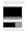
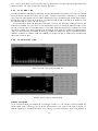
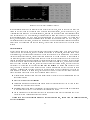
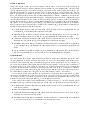

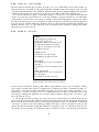
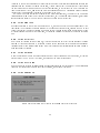

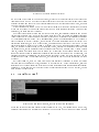
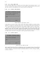
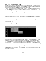
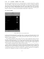
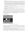
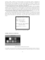
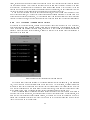
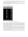
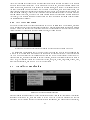
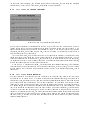
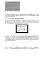
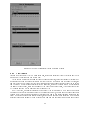

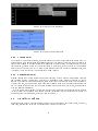
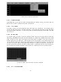
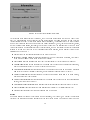
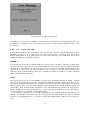
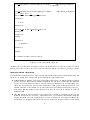
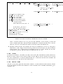
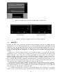
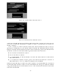
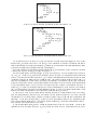
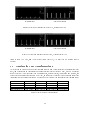
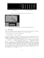
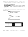
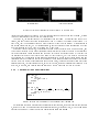
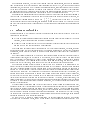
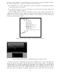
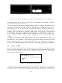
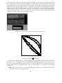
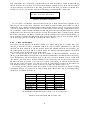
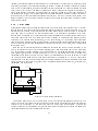


![[U4.72.04] Opérateur CREA_CHAMP](http://vs1.manualzilla.com/store/data/006355027_1-feb0d118e0073065afa5acc9e74a2674-150x150.png)