Download Rev B 28 October 2013 1 The SD16_A as a thermal random number

Rev B 28 October 2013
The SD16_A as a thermal random number-generator
Phil Ekstrom, Northwest Marine Technology, Inc.
The SD16_A analog-to-digital converter module, implemented in some members of the Texas
Instruments MSP430 microcontroller line, can function as a surprisingly good source of randomly
generated bytes, producing them at the rate of four per millisecond. The randomness can be traced to a
fundamentally thermal source, so this is a truly random generator, not a pseudo-random one.
What to do
Configure the SD16_A for maximum gain, input 7 (shorted), and an oversampling ratio of at least 256.
(Smaller may do in some cases - see below). Set the input clock divider to make a 1MHz converter clock
and set the LSBACC bit to give access to the low order part of the converter’s filter register.
When running with a 16MHZ MCLK, C code to accomplish this would be (assuming an appropriate
header file that defines the symbols the same way the User’s guide does):
//1 MHz, (MCLK/16), turn reference generator on.
SD16CTL = SD16XDIV_2 + SD16DIV_0+ SD16SSEL_0 + SD16REFON;
// Oversampling ratio set to 256, enable LSB access, no interrupts,
SD16CCTL0 = SD16OSR_256 + SD16LSBACC;
// Gain = 32 (actually 28), channel is 7 (shorted)
SD16INCTL0 = SD16GAIN_32 + SD16INCH_7;
// Now Go
SD16CCTL0 |= SD16SC;
After each conversion, the SC16IFG flag will set in the SD16CCTL0 register. If you have the interrupt
enabled (by setting SD16IE in that same register) the module will post an interrupt. When the flag sets,
the lower byte of the SD16MEM0 result register contains your new randomly generated byte. Reading
that byte will reset the flag bit. At this clock rate and OSR value, the flag bit will set again with a new
randomly-generated byte every 256 seconds. To access it in C, assign the value in SD16MEM0 to a
variable of type unsigned char.
This recipe assumes that the SD16_A is used for no other purpose. In fact it can be shared with another
use, and configured as a random generator only when needed or when it is free from other demands.
Even when doing its intended job as an ADC for nonzero signals, it will also be generating a noisy byte in
the bottom of its output register as a result of each conversion. If it is run with high gain and an OSR of
at least 256, and if the signal being converted lies safely within its input range limits, one would expect
that the low order byte would be much like it is during dedicated operation. We have not investigated
the quality of that byte in such conditions, but you may find it usable.
As discussed below, you can probably also get away with an oversampling ratio as small as 128, but
there is less theory available to tell you why you should trust it then.
If all you want is a recipe, there it is.
1
Rev B 28 October 2013
How well it works
If we are trying to make a number generator with a uniform distribution, one that produces all possible
values with equal probability, we ought to check its output to see that all values really are produced
about equally often. If we want the generator’s past history to offer no clues about its future actions, we
ought to check the autocorrelation function of the byte sequence to make sure that a large byte value is
not, for instance, usually followed by a small one or vice versa. As will be argued in the appendix, these
are necessary but not sufficient tests for randomness.
To run these tests, we need a file of output bytes from our generator. There is a program in the
appendix which when loaded into the target board of an eZ430_2013 evaluation kit sends out bytes in
start-stop serial form that have been randomly generated by the SD16_A in the manner described
above. It uses the Timer_a module to simulate a serial communication port and runs at 115.2KBaud with
its output on P1.1. I
removed the target
board from the USB
stick hardware of that
evaluation kit, wired it
to a serial-to-USB
interface cable from
FTDI, and read the byte
stream into a PC for
further processing. (The
host program in the PC
is my colleague Ray
Glaze’s work. Thanks,
Ray.)
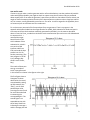
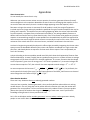
The results of these two
tests on a sample of
N=106 bytes generated
in this manner are shown in the figures at the right.
The first figure shows a
histogram of values
observed in the record,
accumulated by setting
up 256 counters (the
“bins”), one for each
possible byte value,
scanning the record, and
for each value observed
incrementing the
corresponding bin. The
second figure is an
expanded version with
three heavy black lines
indicating the average n
and the average plus and
2
Rev B 28 October 2013
minus the expected standard deviation nn. The average number in each bin is
n  N / 256  10 6 256  3906.25 .
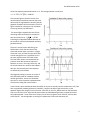
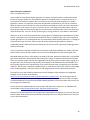
The next two figures show the results of an
autocorrelation calculation based on the same
data record for lags between 0 and 20. (See the
appendix for details of the calculation.) The first
figure includes for comparison the correlation
at zero lag, which is by definition 1.
The second figure expands the scale for the
remaining values and shows for comparison
two horizontal lines at  1 N  0.001
indicating the expected standard deviation of
the results for uniformly distributed randomlygenerated values.
The user’s manual section describing the
SD16 makes it clear that the value of the
converted number does not settle in a single
conversion cycle, and that for two cycles after
a value changes there is a significant error in
the most significant bits of the ADC result.
The new value remains correlated with the
previous value. We would not expect this
behavior to occur in the noisy lower bits, and
the results shown here confirm that indeed it
does not. Successive bytes in the sequence
are effectively uncorrelated.
.
The appendix contains a pointer to a suite of
tests offered by NIST for candidate random
number generators, and to the “Dieharder”
test suite, a more convenient implementation
of those tests along with several others.
It also contains some rude words about the ability of any test to actually confirm randomness. Still, if we
have a supposedly random generator of numbers, it ought to be able to pass those tests, as the
appendix argues they should, most of the time. We have run the STS_SERIAL test from the Dieharder
suite on a set of thirty 105-byte records derived from the USB-adapted generator, and we found that
they indeed passed – most of the time. Twenty nine of the trials gave a result “Passed”, and one was
called “Weak”. See the appendix on testing for randomness if that result distresses you.
3
Rev B 28 October 2013
Why it works at all
Every time a capacitor is connected to a resistive source, allowed to settle, and then disconnected it
acquires a randomly generated voltage with standard deviation VRMS  kT C in addition to whatever
intentional voltage the source is providing. This random addition is called “contact noise”, but it is
actually the resistor that is noisy, not the contact, as explained in the appendix. Here k is Boltzmann’s
constant and T is the absolute temperature, so at room temperature this becomes VRMS  64V
for C in pF.
C
Every microsecond when the input sampler of the SD16_A contacts the external circuit and the voltage
on its 20pF sampling capacitor settles to a new measurement of the nominally zero input value, plus or
minus “contact noise” that has a standard deviation of 64/20 = 14 microvolts. That voltage is amplified
by a factor of 28, to 0.4mV, and applied to the sigma-delta modulator. In the course of the conversion,
256 of these values will be more-or-less averaged by the digital filter, to yield a random contribution no
smaller than 400/25625V. This truly-random addition could approach this theoretically smallest
value if the filter simply averaged. In fact it does something more complicated to minimize the shaped
quantization noise of the second order delta modulator, so we expect that there will be more of the
truly random noise than this minimum.) For OSR = 256, the most significant bit of the output register is
bit 23 (see figure 26-5 of the MSP430F2xxx User’s guide, SLAU144J), and that bit is worth 600 mV. The
least significant bit of the register is therefore worth 2-23 *600 mV72nV. That means the 25V noise
contribution is worth at least 25V/72nV = 350 LSB, and we expect it to be Gaussian noise, distributed
along the familiar bell-shaped curve of probability density.
The simple treatment in the paragraph above requires some assumptions about just how the input
amplifier and delta modulator are constructed and operated. Based on the gain and capacitance
specifications and the fact that the module still offers gain when the active amplifiers are omitted, I have
assumed that each of the two Cs capacitors (10pF at gain 32) in figure 26-2 of theF2xx users guide
(SLAU144J ) is made of eight 1.25pF capacitors (like the one that is used at gain 1) that are charged in
parallel and then connected in series when presented to the ADC core. A final factor-of-four gain is
achieved some other way, perhaps in the delta modulator, or perhaps by actually splitting each of the
1.25pF capacitors four ways. There are other ways that the input amplifier could be operating, but most
of them lead to the same noise estimate. None I have thought of leads to a smaller one.
As we will see, the output is actually noisier than this estimate would lead us to expect, but that’s moreor-less OK even though it is not quite clear just where that is all coming from. We only need a guarantee
of enough thermal noise to make things genuinely random, to fill up the lower byte with “good” noise
known to originate in a thermal source that we expect to have a Gaussian distribution.
To check on this noise estimate, a program was written for the eZ430F2013 that accumulated statistics
on the SD16_A output in the upper (normal) section of the SD16 output register. For comparison, we
need a prediction based on our noise model above for what we should expect. The MSB of the upper
output register is worth 600mV at Gain=1, so its LSB is worth 600mV*2-15 = 18V. At any other gain it is
worth 18V/G. Our simple model of the filter effect is that it will simply average the noise samples, so
we expect them to be attenuated by a factor of 1 / OSR Thus we predict a noise in f the upper register
equal to
64V
G
C 18V
1
OSR
 3.6
G
OSR  C
LSB.
4
Rev B 28 October 2013
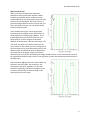
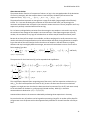
Plotting this out vs.
G / C for the
various available gain
settings (tick marks
on the traces) and
interesting values of
OSR, we obtain the
figure on the right.
Running a program in
an eZ430F2013 to
calculate the mean
and standard
deviation of 106
conversions for each
of those cases gives
instead the next figure. It has approximately the same shape, but the measured values are about four
times larger than the predicted ones. If we knew where all that came from and how securely it was tied
to a thermal source, perhaps we could confidently use a smaller OSR and generate bytes more rapidly.
As things stand, this
note recommends
OSR=256.
One of the author’s
major goals in writing
this note is to lure
some of the SD16
design team into
commenting on this
comparison and
revising the previous
several paragraphs –
all in aid of making
more secure the
theoretical
foundations of the
scheme and perhaps making it faster by leaving us more comfortable with smaller values of OSR.
5
Rev B 28 October 2013
Why it works so well
When you have a set of data with a Gaussian
distribution and you take those numbers modulo
something comparable with or smaller than their
standard deviation, the result always comes out to be
nearly uniformly distributed. That is the real key; if
you have enough Gaussian noise to fill your byte, you
don’t care about much else. The rest of this section
will show how that works.
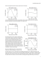
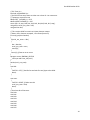
In the example at the right, we see some graphs
illustrating how that begins to take effect, where in
these graphs we are taking things modulo 1. In our
present application we can think of that unit 1 as
being one byte. In the first figure the standard
deviation of the Gaussian is less than half a byte – still
a bit small - but when you take the ordinate of the
curve modulo 1, that is when you slice it along each of
the vertical green lines, superimpose those slices, and
add them up as has been done with the dashed lines
on the left side of the graph, you get a sum (heavy
black line) that is not yet flat, but already has sharply limited variation. In this illustration the mean of
the original distribution has been chosen ¼ unit off-center to cause the maximum possible variation in
the black trace.
Well, how about adding a little more noise? When the
Gaussian is only 20% wider, the variations in the
heavy black trace shrink markedly. Let’s plot that
black trace separately, and follow its behavior as we
increase  (and thereby increase the width of the
Gaussian) by a few more steps.
6
Rev B 28 October 2013
The first two graphs represent the two cases shown in full above.
As the standard deviation increases, the probability density rapidly flattens out until its variation
becomes completely invisible when plotted at the original scale.
Now plotting that last case again but allowing the
vertical scale to adjust we see that the shape of the
variation has not changed, but that its scale has
become so small as to be undetectable in practice.
To get that degree of flatness takes a standard
deviation of 0.7 times the modulus value. For data
taken modulo one byte, that requires 180 LSB of
noise standard deviation. More noiseis better, so
long as it all stays within the input range of the ADC;
our OSB=256 case, with a contact noise contribution
of 350LSB, is safe by a wide margin.
But there is additional value to an extremely flat
distribution made by folding up a Gaussian as we
have done above; you can’t easily disturb it by adding something else to it. Adding something to the
input of the ADC just moves the mean of the input Gaussian distribution. But when the resulting output
distribution is flat, then the location of the original Gaussian’s peak no longer matters. All that moving
the peak could ever do was to move the location and change the height of that wavy trace we have
7
Rev B 28 October 2013
been watching. If the wave has a small enough amplitude to be undetectable, then the effect of a
change in the mean of the noise is also undetectable.
That is the starting point for a useful way to think about other contributions to our noise generator’s
result. All that any additive (interfering) signal can do is to move that mean. If it moves the mean and
leaves it in a new location, then quite clearly it has no effect on the performance of our generator. If it
moves it back and forth between conversions, we still won’t have any way to tell that it has done so or
any reason to wish that it hadn’t. If it changes back and forth during a conversion, we expect that all it
can do is to broaden the noise distribution, and as we can see that helps us out. Once we have enough
Gaussian noise, it looks like we can relax about interference. So long as the SD16_A is well enough
shielded to do its normal ADC function, it should be able to make high quality noise bytes.
So much for external noise sources. However the S-D modulator will respond to the input noise and its
own quantization noise can become correlated with the contact noise. This possibility could take us into
regions of sigma-delta converter design that I do not propose to enter. The contribution of an S-D
designer would be welcome, but I will take it no farther, beyond noticing that this proposed use of the
SD16A does appear to work remarkably well, so seems not greatly harmed by that possible effect.
It is worth noting that we do need the SD16_A
to be working well as an ADC, and as already
mentioned we need the entire input noise
voltage range to fit within its linear input range.
If one tail of the input noise gets outside the
linear range of the ADC function, we can no
longer guarantee a flat noise spectrum in the
result, as illustrated in the plot at the right. The
output noise spectrum in the case illustrated
here has a distortion that is just the negative of
the missing tail of the original distribution.
When the SD16_A is operating with its input
range symmetric around zero, and with the
input shorted as we do here, that requirement
is easily met and the situation diagrammed here
is easily avoided.
Conclusion
The SD16_A sigma-delta ADC can be operated as an excellent random generator of bytes, where the
source of randomness can be traced to thermal noise.
8
Rev B 28 October 2013
Appendices
About Contact Noise
It is not actually the contact that is noisy.
Whenever you connect a warm resistor across a capacitor, the resistor generates Johnson (thermal)
noise and applies it to the capacitor. Meanwhile the same resistor is discharging that capacitor. As the
net result of those two actions, there is a random voltage appearing across the capacitor, which
fluctuates as long as the resistor is connected. If the RC product is small, the range of frequencies
involved may be very large and mostly outside the passband of a typical sensitive amplifier that may be
looking at the capacitor. The amplifier may see nothing happening. When the resistor is disconnected
from the capacitor, as happens every microsecond in the SD16_A, the voltage suddenly freezes at a
definite value and can be seen by narrow-band circuitry. Since a new frozen value appears any time the
capacitor is contacted long enough for a new equilibrium to be established, the effect has acquired the
name contact noise even though the switch contact is not actually the source of the noise. The electrical
resistance of the switch and circuit is the actual source, and what it contributes is thermal noise.
An electrical engineering text which analyzes this effect might proceed by integrating the Johnson noise
spectrum over the bandwidth defined by the resistor and capacitor considered as a single-section lowpass filter, and thereby derive an expression for how much noise to expect. That is complicated; we
won’t do it that way.
A physicist looking at the same problem would more likely think about the Equipartition Theorem from
Statistical Mechanics. It states (roughly) that any quadratic energy term in a system will have an average
energy equal to kT/2 when the system is in thermal equilibrium. In our case, we notice that the voltage
across a capacitor C gives rise to an energy term ½ CV2 which is quadratic in V, its terminal voltage. We
can set that term equal to ½ kT, then solve for the mean-squared terminal voltage  V 2  kT / C .
At room temperature this becomes Vrms   V 2   kT / C  64V C for C in picofarads, the
result quoted in the body of the note. The 20pF input capacitor of the SD16_A will have an rms thermal
noise voltage due to this effect of 64V
20  14V .
About Random Numbers
There aren’t any. However there are randomly generated numbers.
Once you have a number, however generated, it has a perfectly definite value and there is nothing
random about it. The only thing that can be random about the situation is the way the number was
generated. For most purposes it is fair to call that process truly random if there is no way to predict
(better than chance) the number that the generator is going to make next - even if you have full
knowledge of the generator’s history and internal state.
So it is fair to talk about random number-generators, but not random-number generators. Mostly,
people are not careful about that distinction, but this note will try to be.
9
Rev B 28 October 2013
About Testing for Randomness
There is no good way to do it.
In the output from a perfectly random generator of numbers, at least one with a uniform distribution
like we are trying to make here, all possible bit sequences are equally likely. A string of all ones or all
zeros looks to us wildly non-random, but it is as likely as any other particular sequence in a random
generator’s output. In a single-byte result from the generator proposed here, you will see a solid zero
about 15 times a second. You will see a pair of two zero bytes together more-or-less every 16 seconds, a
trio of three in a row more or less every 72 minutes, four in a row about every twelve days, and so on.
No particular sequence of the same length that you could name would be either more or less likely than
one with all bits zero. You can’t call any of them right or wrong, random or non-random in themselves.
What you can do is to test for properties that a large majority of randomly generated sequences is likely
to have, realizing that any such test will sometimes call foul on a sequence that came out of a perfectly
random generator. A truly random generator must eventually make all possible sequences – including all
of those that fail your test. Also, there may also be chaotic sequences generated by a perfectly
predictable (pseudo-random) process that always pass such a test, which a genuinely random generator
could not always do.
In short, a generator that fails a sensible test consistently is with high probability not random. One that
passes may or may not be truly random. So we can test for failed generators, but not for good ones.
We talked about two tests in some detail in the body of this note, based on the ideas that: 1) all possible
byte values should occur about equally often and 2) pairs of bytes in sequence should be uncorrelated.
These are relatively simple tests that are suggested by the physical process that we expect is going on in
our generator. They characterize that process, which appears to be fundamentally unpredictable, and
they give this physicist writer a good feeling. They are also likely to catch a programing error should we
make one. But they are not tests for randomness per se. Assurance of that has to come from knowledge
of the underlying physics, and of the electronic and computational structure built atop that physics.
That said, there are some widely accepted tests that are thought to have relevance to cryptographic
strength. A suite of them can be found at
http://csrc.nist.gov/groups/ST/toolkit/rng/documentation_software.html. Any random generator of
numbers that we want to take seriously ought to be able to pass them, at least most of the time. Again,
as should be obvious from the fact that pseudo-random generators can also pass them, they too are not
tests for genuine randomness.
A more convenient implementation of some of these and other tests, ready to run on a Windows PC,
can be found at http://www.phy.duke.edu/~rgb/General/dieharder.php
We have run 105-byte sequences from the generator proposed here through the sts_serial test from this
suite and have obtained the results mentioned in the body of the note: they pass most but not all of the
time, as we should expect.
10
Rev B 28 October 2013
About Autocorrelation
The autocorrelation function of a sequence of values xj at lag L is the averaged product of the deviations
of x from its average, with the samples chosen L intervals apart, divided by the variance of the
sequence. That is, r L  ( x j  L   )  ( x j   )  /  x j    x j   



The pointed brackets represent an average over a range of the index j large enough to be effectively
infinite. If L = 0 we are calculating the correlation of each value of with itself; not surprisingly the
numerator and denominator are equal in that case and answer comes out 1 for any sequence at all. Any
sequence is perfectly correlated with itself at zero lag.
For L >0 we are asking whether variations from the average in one sample are mirrored in any way by
the variations from average of the sample L time intervals later. If the sequence generator is purely
random, the correlation for any lag L>0 calculated over an infinite sample should be infinitely small.
But we do not have infinite sample sizes available, and when working with a small processor we may
need to calculate a finite approximation to the autocorrelation efficiently. Paying attention to samples
lost at the ends of the record and to the fact that the set of samples in the two factors are slightly
different and may have slightly different averages, we recast the result above in terms of sums over a
finite sample of size N as

1 N L
1 N
 1  N
,
,
x


x


C
L


  x j  L   A   x j   B  and finally


j
B
j
N  L j 1
N  L jL
 N  L  j  L

r ( L)  C ( L) / C (0) .
A 
The expression for the Covariance C(L) can be expanded and simplified as:
N
N

1  N






  x j  L  x j   B  x j  L   A   A  x j   B   N  L  B  A 
 N  L  j  L
jL
jL


C L   

 1  N

  x j  L   x j    B  A   B  A   B  A
 N  L  j  L


 1  N

  x j  L   x j    B  A
 N  L  j  L

This simplification depends upon recognizing two of the sums in the first expansion as identical to  A
and  B .The final result expresses the result for C(L) in terms of three sums that can be calculated
together in a single pass over the data; the data record can be processed “on the fly” and never stored,
so the calculation can be done in a processor with limited memory. With C(L) in hand the
autocorrelation is obtained as r ( L)  C ( L) / C (0) .
Autocorrelation values in the note were obtained by evaluating these expressions in that way.
Do note that the sum of products can be large when processing a large file. A random million-byte file
will generate a sum of squares with a value approximately 1282x106234 that will overflow a four-byte
field.
11
Rev B 28 October 2013
Program for the eZ430-F2013
The program below loaded into an eZ430-F2013 will send randomly generated bytes in start-stop serial
format at 115.2 KBaud out through P1.1, which is pin 3 of the MSP430F2013 processor included in the
eZ430-F2013 . The oversampling ratio may be changed by altering a statement just below the comment
line // SD_16. However notice the warning message just above that line. The program works as
described in the text only for OSR >= 128. For smaller oversampling ratios, characters are produced
faster than they can be sent, and successive characters in the serial communication output no longer
represent successive characters in the generator output.
There are two separate files below, Main.c and Timer_A.c. They were compiled using IAR Embedded
Workbench.
//Main.c
// Random Number generator test, target is MSP430F2013,
#include <msp430f2013.h>
int send_byte(char);
unsigned char Datum;
volatile unsigned int v = 0;
int main( void )
{
// Disable watchdog timer
WDTCTL = WDTPW + WDTHOLD;
// Set DCO to 16MHz, which is OK at 3.3V Vcc.
// Active current about TBD MA at 16MHz and 3.3V
BCSCTL1 = CALBC1_16MHZ;
DCOCTL = CALDCO_16MHZ;
// Configure the ports
//P1
P1OUT = 0; // Outputs are low
P1DIR = 0xFF; // All pins are output
P1SEL = BIT1; // And Bit1 is timer output.
//P2
P2OUT = 0;
P2DIR = 0;
P2REN = 0xFF;
// Timer_A
// P1.1 = data output Pin 3 of DIP package. (LED is P1.0, pin 2)
TACCR0 = 139;
// = 16 MHz/115.2 KBaud
TACCTL0 = OUTMOD_1 + CCIE; // Set on event, enable interrupt;
TACTL = TASSEL_2 + ID_0 + MC_1;
12
Rev B 28 October 2013
// This SHIFT definition is the SD_16 register position from which the
// LSBit of the data byte is taken. SHIFT <= 8. Ordinarily 0 or 8.
#define SHIFT 0
// It and the oversampling ratio set below define the case.
// OSR >= 128 assumed so bytes are sent faster than they are produced.
// SD_16
//1 MHz, (MCLK/16), turn reference generator on.
SD16CTL = SD16XDIV_2 + SD16DIV_0+ SD16SSEL_0 + SD16REFON;
// Oversampling ratio set, enable LSB access, no interrupts,
SD16CCTL0 = SD16OSR_256 + SD16LSBACC;
// Gain = 32, channel is 7 (shorted)
SD16INCTL0 = SD16GAIN_32 + SD16INCH_7;
// Now Go
SD16CCTL0 |= SD16SC;
//***************************************
v = SD16MEM0; // Clear any leftover data.
//*******************************************************************
__enable_interrupt();
// Event loop starts here
while(1)
{
// Wait for next value
while((SD16IFG & SD16CCTL0) == 0) v++;
// Shift during this assignment to move up the filter register.
Datum = SD16MEM0>>SHIFT;
send_byte(Datum);
} // End the event loop.
} // end main
13
Rev B 28 October 2013
// File Timer_A.c
#include <msp430f2013.h>
// Set TACCTL0 to one of these to either set or clear P1.1 on next event.
// Temporary reversal for test
#define SET OUTMOD_1 + CCIE
#define RESET OUTMOD_5 + CCIE
enum {idle = 0, start, bit0, bit1, bit2, bit3, bit4, bit5, bit6, bit7, stop};
unsigned int serial_out_state = idle;
unsigned char Out;
// This routine called from main to initiate character output
// Return 0 for character accepted, 1 for refused (overrun).
int send_byte(char Outchar)
{
if(serial_out_state == idle)
{
Out = Outchar;
serial_out_state = start;
return(0);
}
return(1); //Overrun error return
}
#pragma vector=TIMERA0_VECTOR
__interrupt void Timer_A0( void )
{
switch(serial_out_state)
{
case idle:
{
TACCTL0 = SET; // Set Idle line and wait for send_byte to be called.
break;
}
case start:
{
TACCTL0 = RESET; // Make start bit
serial_out_state = bit0;
break;
}
// Send next bit of character.
case bit0:
case bit1:
case bit2:
case bit3:
case bit4:
case bit5:
case bit6:
case bit7:
14
Rev B 28 October 2013
{
if((Out&0x01) == 0) TACCTL0 = SET; // if bit is 0, output is 1
else
TACCTL0 = RESET; // and vice versa.
Out=Out>>1;
// shift to next bit
serial_out_state++;
// increment to next state.
break;
}
case stop:
{
TACCTL0 = SET; // Set Idle line and
serial_out_state = idle; // go to idle state.
break;
}
default:
{
serial_out_state = idle;
break;
}
} //End switch(serial_out_state)
} //End __interrupt void Timer_A0( void )
15