1
YMAP: a pipeline for visualization of copy number
variation and loss of heterozygosity in eukaryotic
pathogens
Abbey et al.
Abbey et al. Genome Medicine 2014, 6:100
http://genomemedicine.com/content/6/11/100
Abbey et al. Genome Medicine 2014, 6:100
http://genomemedicine.com/content/6/11/100
SOFTWARE
Open Access
YMAP: a pipeline for visualization of copy number
variation and loss of heterozygosity in eukaryotic
pathogens
Darren A Abbey1, Jason Funt2, Mor N Lurie-Weinberger3, Dawn A Thompson2, Aviv Regev2, Chad L Myers4
and Judith Berman1,3*
Abstract
The design of effective antimicrobial therapies for serious eukaryotic pathogens requires a clear understanding of
their highly variable genomes. To facilitate analysis of copy number variations, single nucleotide polymorphisms
and loss of heterozygosity events in these pathogens, we developed a pipeline for analyzing diverse genome-scale
datasets from microarray, deep sequencing, and restriction site associated DNA sequence experiments for clinical
and laboratory strains of Candida albicans, the most prevalent human fungal pathogen. The YMAP pipeline (http://
lovelace.cs.umn.edu/Ymap/) automatically illustrates genome-wide information in a single intuitive figure and is
readily modified for the analysis of other pathogens with small genomes.
Background
The collection of large, near-comprehensive genomic datasets of human pathogens such as Candida albicans has
become common due to the availability of next-generation
sequencing technologies. A major challenge is to represent
these large, complex datasets that probe a heterozygous
diploid genome in a manner that is biologically relevant and
easy to interpret. In C. albicans, genome changes of small
scale (single nucleotide polymorphisms (SNPs), short insertions, and short deletions) and large scale (duplications,
deletions, loss of heterozygosity) can have important consequences in the development of new clinical phenotypes,
most notably, drug resistance [1,2].
The C. albicans genome has eight linear chromosomes
that are highly heterozygous (approximately 70K SNPs between homologs), compact (0.9 to 3.2 Mbp) and are not
detectable via microscopy-based karyotyping methods.
Contour-clamped homogenous electric field (CHEF) electrophoresis provides information on relative chromosome
sizes but is time consuming, low throughput, and not
definitive without additional Southern blot analyses of
* Correspondence: [email protected]
1
Department of Genetics, Cell Biology and Development, University of
Minnesota, 6-160 Jackson Hall, Minneapolis, MN 55415, USA
3
Department of Molecular Microbiology and Biotechnology, Tel Aviv
University, 418 Britannia Building, Ramat Aviv 69978, Israel
Full list of author information is available at the end of the article
individual probes for different chromosome regions. Thus,
whole genome analyses via microarrays, deep sequencing,
or sequence sampling methods, such as double-digest
restriction-site associated DNA sequencing (ddRADseq),
have the potential to improve the speed and precision of
genome analysis.
Mapping of small yeast genomes was pioneered in
Saccharomyces cerevisiae, which has 16 very small chromosomes (0.2 to 1.5 Mbp), point centromeres spanning
only approximately 100 bp and short telomere repeats
that span approximately 300 to 400 bp, a single rDNA
locus containing approximately 150 tandem repeats, and
no other major regions of repetitive DNA [3]. C. albicans, like higher organisms, has regional, epigenetic centromeres that are relatively small (3 to 5 kbp compared
with 0.5 to 10 Mbp in humans) [4,5], telomere repeats
that span several hundred base pairs [6] and a set of
telomere-adjacent genes (TLO1 to TLO16) found at
most chromosome ends [7,8]. In addition to the single
rDNA locus that includes 25 to 175 tandem repeats, C.
albicans chromosomes each carry one or two major
repeat sequences composed of nested repeat units that
span 50 to 130 kbp [9,10]. Several different categories of
transposons and long terminal repeats are also scattered
throughout the chromosomes. In C. albicans, as in
human cancer cells and some normal human tissues,
© 2014 Abbey et al.; licensee BioMed Central Ltd. This is an Open Access article distributed under the terms of the Creative
Commons Attribution License (http://creativecommons.org/licenses/by/4.0), which permits unrestricted use, distribution, and
reproduction in any medium, provided the original work is properly credited. The Creative Commons Public Domain
Dedication waiver (http://creativecommons.org/publicdomain/zero/1.0/) applies to the data made available in this article,
unless otherwise stated.
Abbey et al. Genome Medicine 2014, 6:100
http://genomemedicine.com/content/6/11/100
DNA copy number and color schemes provide allele
status information with data plotted either vertically for
an individual strain or horizontally to facilitate comparison between individuals.
The YMAP website is available for use at [27] and
includes some example datasets as well as decision flowdiagrams to help determine if the pipeline will be able to
process your data (Additional file 1). The source files and
directory organization needed for installing the pipeline
on your own server can be downloaded from [28].
Implementation
The genome analysis pipeline is composed of three main
components: a module that performs raw sequence
alignment and processing (Figure 1, steps 1 to 3), a module that performs custom CNV and SNP/LOH analyses,
and a module that constructs figures summarizing all
completed analyses and then displays them on the webpage. The implementation details for each of these components are described in more detail in the following
sections. The accession numbers for the sequence data
for strains analyzed can be found at NCBI (BioSample
accessions 3144957 through 3144969).
The first component of the central computation engine
takes the user-input data and attempts to correct some
typical file errors before outputting corrected FASTQ file
(s) for use by later steps in the pipeline. Typical sequence
1. FASTQ file cleaning.
2. BAM file construction.
3. PILEUP file construction.
5. SNP/LOH analysis.
Custom
analysis
4. CNV analysis.
Rawsequence
processing
aneuploid chromosomes appear frequently and in some
cases specific aneuploidies or genome changes are
diagnostic of specific changes, such as the acquisition of
drug resistance [1,11]. Thus, the ability to detect karyotype changes in the C. albicans genome can facilitate
informed choices regarding therapeutic strategies.
Most available tools for genome analysis were designed
primarily to analyze human genome sequence data and
assist in disease diagnosis. Many tools identify short-range
variations in next-generation sequence datasets (reviewed
in [12,13]). Most tools that produce a visualization primarily represent one major aspect of a genome: rearrangements (for example, CIRCUS [14], inGAP [15], Gremlin
[16]) or large CNVs (WISECONDOR [17], FAST-SeqS
[18]). Few tools provide a whole genome view of the calculated genome changes in a single glance/figure. ChARM
[19] detects and visualizes copy number changes in microarray datasets. CEQer [20] and ExomeCNV [21] process
and visualize copy number changes in exome-only sequence data. One of the most versatile visualization tools,
IGV [22,23], can display different types of genomic variants (for example, copy number variation (CNV), SNPs,
loss of heterozygosity (LOH), sequence coverage, among
others), but visualization is limited to one genomic phenotype at a time, and thus it is not readily applied to time
series data. Further, when applied across the entire
genome view, as opposed to single chromosome views,
other genomic features (that is, centromeres, telomeres,
repetitive sequence elements) are not displayed.
Here we present YMAP, a genome analysis pipeline
motivated by the need to analyze whole genome data in
a manner that provides an overview of the entire genome, including major changes in CNVs and allele ratios
(LOHs) that it has undergone. As such, YMAP utilizes
and extends existing tools for both short- and longrange genome analyses to provide a whole-genome view
of CNVs and LOHs in small genomes, using C. albicans
as a test case. YMAP is designed to be amenable to the
analysis of clinical as well as laboratory isolates and to
be readily adapted for the study of genome organization
in other pathogenic yeast species. For genomes with
known haplotypes, YMAP utilizes a color scheme to
visualize the allele specificity of segmental and whole
chromosome LOHs. For new genomes such as clinical
isolates, it visualizes LOH events and, with appropriate
homozygosed derivatives, it facilitates the construction
of haplotype maps (hapmaps) [24]. Originally designed
to process microarray data that include both SNP and
comparative genomic hybridization (CGH) data [25],
YMAP accepts several types of whole genome datasets.
YMAP processes paired- and single-end whole genome
sequence, as well as paired- and single-end ddRADseq
data, which samples a sparse number of genomic loci at
low cost per sample [26]. Dense histograms indicate
Page 2 of 15
6. Figure construction.
Figure 1 Conceptual overview of YMAP genome analysis pipeline.
The central computation engine of the pipeline has three major
components: raw sequence processing, custom analysis, and
figure construction/presentation.
Abbey et al. Genome Medicine 2014, 6:100
http://genomemedicine.com/content/6/11/100
data are input as one or two (for paired-end reads)
FASTQ format files, either raw or compressed in the ZIP
or GZ format. Depending on connection reliability,
uploading a 500 Mb compressed file can take from minutes to a few hours. The large size of FASTQ files leaves
them prone to file transfer errors that result in corruption
because the file format does not have an internal error
correction/identification system. This corruption often
results in the final read entry being incomplete, which can
cause analysis programs to crash, and normally has to be
dealt with on a case-by-case basis. The size of the
uploaded file is available in the ‘Manage Datasets’ tab
beside the dataset name. Users can thus manually check
whether the uploaded file size is equal to the expected file
size. The issue of transfer errors is partially dealt with internally by trimming the FASTQ file to remove incomplete entries. Trimming the longer of the paired-end
FASTQ files to the length of the shorter file is also done
to deal with single-end reads that are generated by some
sequencing technologies. Both steps are done through inhouse scripts (available at [28]; incomplete entry removal:
sh/FASTQ_1_trimming.sh or unbalanced reads: sh/FASTQ_2_trimming.sh).
The second step in the central computation pipeline is
to process the corrected FASTQ file into a final Binary sequence Alignment/Mapping (BAM) file. The single- or
paired-end reads are aligned to one of the installed reference genomes using Bowtie2 with SAM output mode set
to ‘very sensitive’ [29], resulting in a Sequence Alignment/
Mapping (SAM) file. SAMtools [30] is used to compress
this into a BAM file. PicardTools [31] is used to
standardize the read-group headers in the BAM files, to
resolve some formatting irregularities to the BAM file.
SAMtools is then used to sort the BAM file, which is required for efficient later processing steps. FASTQC [32] is
used to identify the quality coding system used in the input FASTQ files, as a prelude to defining the input parameters for processing by the Genome Analysis ToolKit
(GATK) [33], which performs indel-realignment of the
BAM files, removing spurious apparent SNPs around true
indels in the primary alignment. Settings for all outside
tools can be found in the source code on sourceforge [28]
by looking at the sh/project.paired_*.sh and sh/project.single_*.sh shell scripts.
The third step in the sequence data processing component of the pipeline is to convert the BAM file into a simpler text file containing limited data for each coordinate
across the genome, which simplifies later processing. The
SAMtools function mpileup first processes the BAM file
into a ‘pileup’ file, which contains information about all of
the mapped reads at each chromosome coordinate in a
simple format that facilitates subsequent processing by
custom Python scripts (available at [28] in the ‘py’ directory). The Python scripts extract base call counts for each
Page 3 of 15
coordinate, discarding indel and read start/end information. The raw read-depth data per coordinate is saved to a
text file [‘SNP_CNV.txt’] that is input into the CNV analysis section of the pipeline. Any coordinates with more
than one base call have that information saved to a separate text file [‘putative_SNPs.txt’] that is input into the SNP
and LOH analysis section of the pipeline. These two files
can be downloaded after being made in the ‘Manage
Datasets’ tab by selecting either ‘SNP_CNV data’ or
‘putative_SNP data’ beside the relevant dataset name.
Detailed flow diagrams explaining the processes each
file goes through upon introduction to YMAP are available in Additional files 2, 3, 4, and 5.
Copy number variation analysis
CNV analysis of next-generation sequencing data by the
pipeline is based upon read depth across the genome. Several biases can impact read depth and thereby interfere
with CNV analysis. Two separate biases, a chromosomeend bias and a GC-content bias, appear sporadically in all
types of data examined (including microarray and whole
genome sequencing (WGseq) data). The mechanism that
results in the chromosome end artifact is unclear, but the
smooth change in the apparent copy number increase
towards the chromosome ends (Figure 2A) suggests that
some DNA preparations may release more genomic DNA
as a function of telomere proximity (Jane Usher, personal
communication). A GC-content bias is due to strong
positional variations in GC content in the C. albicans
genome. This, combined with the PCR amplification bias
introduced during sequence library or array preparation,
results in a strong positional effect in local copy number
estimates (Figure 3A). In datasets produced from the
ddRADseq protocol, a third bias is associated with the
length of restriction fragments. A fourth bias, seen consistently in all ddRADseq data sets, appears as a high
frequency of short-range increases and decreases in read
depth at specific genome positions across all strains
analyzed, and thus can be removed by normalization to a
control dataset from the reference genome. The YMAP
pipeline includes filters, which can be deselected by the
user, for each of these biases to correct the data before
final presentation and to facilitate detection of bona fide
CNVs. The final presentation of the corrected copy number data is in the form of a histogram drawn vertically
from the figure centerline (Figures 2A,B, 3A,B, and 4A,B).
The chromosome-end bias is normalized using locally
weighted scatterplot smoothing (LOWESS) normalization
[37] of average read depth versus distance to the nearest
chromosome end, for 5,000 bp windows tiled along each
chromosome (Figure 2C). The LOWESS fitting is performed with a smoothing window size determined for each
dataset as that which produces the least error between the
fit and the raw data, using 10-fold cross-validation [38].
Abbey et al. Genome Medicine 2014, 6:100
http://genomemedicine.com/content/6/11/100
Page 4 of 15
A
B
C
D
Corrected
Normalized
CNV estimate
Normalized
CNV estimate
Raw
250Kb
500Kb
750Kb
250Kb
1000Kb
500Kb
750Kb
1000Kb
Distance to chr end.
Distance to chr end.
Figure 2 Normalization of chromosome-end bias. (A,B) Black bars up- and down-wards from the figure midline represent local copy number
estimates, scaled to genome ploidy. Different levels of grey shading in the background indicate local changes in SNP density, with darker grey
indicating more SNPs. Detailed interpretations are similar to those described in [25]. (A) Map of data with chromosome end bias present in
read-depth CNV estimates for strain YQ2 dataset (from EMBL-EBI BioSamples database [34], accession SAMEA1879786). (B) Corrected CNV
estimates for strain YQ2 mapped across all C. albicans chromosomes. (C,D) Raw and corrected normalized read-depth CNV estimates relative
to distance from chromosome ends. Red, LOWESS fit curve.
A
B
C
D
Corrected
Normalized
CNV estimate
Normalized
CNV estimate
Raw
20%
40%
60%
% GC content
80%
100%
20%
40%
60%
80%
100%
% GC content
Figure 3 Normalization of GC-content bias. (A) GC-content bias present in read-depth CNV estimates using WGseq for strain FH6.
(B) Corrected CNV estimates mapped across FH6 genome. (C,D) Raw and corrected normalized read-depth CNV estimates versus GC content.
Red, LOWESS fit curve. Chromosome illustrations are as in Figure 2.
Abbey et al. Genome Medicine 2014, 6:100
http://genomemedicine.com/content/6/11/100
Page 5 of 15
A
C
Normalized
CNV estimate
B
Raw
3
2
1
100bp
200bp
300bp
400bp
500bp
600bp
700bp
800bp
900bp
800bp
900bp
D
Normalized
CNV estimate
ddRADseq Fragment Length
Corrected
3
2
1
100bp
200bp
300bp
400bp
500bp
600bp
700bp
ddRADseq Fragment Length
Figure 4 Normalization of fragment-length-bias in ddRADseq data. (A) High noise of raw read-depth CNV estimates in CHY477 [35] ddRADseq
data with GC-content, fragment-length, and position-effect biases. (B) CNV estimates mapped across the genome and corrected for GC bias, fragment
length bias and normalized to the reference data. (C) Average read-depth CNV estimates versus predicted restriction fragment length for strain RBY917
Mata/a -his, -leu, delta gal1::SAT1/GAL1 derived from SNY87 [36]. Black, LOWESS fit curve. (D) Corrected average read-depth CNV estimates versus
fragment length, with regions of low reliability data in red, as described in more detail in the text. Chromosome illustrations are as in Figure 2.
Dividing the raw data by the fit curve normalizes the bias
(Figure 2D), allowing an unimpeded view of the mapped
genome (Figure 2B, a diploid with no significant CNVs).
Because this bias is sporadically present, the correction is
optional and is not performed by default.
The GC-content bias is normalized using LOWESS
normalization of average read depth versus GC content,
for 5,000 bp windows tiled along each chromosome
(Figure 3C). The LOWESS fitting is performed with a
smoothing window size determined for each dataset as
that which produces the least error between the fit and
the raw data using 10-fold cross-validation. Dividing the
raw data by the fit curve normalizes this bias (Figure 3D),
allowing an unimpeded visual examination of CNVs
across the genome. For example, it can distinguish
chromosome number for a near-tetraploid strain with a
small segmental duplication near the centromere of
ChrR, three copies of chromosomes 4, 5R and 6, and
with seven copies of the left arm of chromosome 5R
(due to the presence of three copies of whole Chr5 and
two copies of an i(5L) with two copies of Chr5L per isochromosome) (Figure 3B). Because this bias is always
present to some degree in all data types examined, the
correction is performed by default unless deselected by
the user.
The ddRADseq protocol generates high read depths at
a sub-sampling of genomic loci, resulting in a muchreduced total cost per strain sequenced. The protocol
produces a library of restriction fragments digested with
two different restriction enzymes (in this case MfoI and
MpeI). A strong bias exists in the read depth versus the
length of each valid restriction fragment (obtained via a
simulated digest of the reference genome, followed by
selecting fragments that have the two restriction
fragment ends; Figure 4C). The fragment-length-bias is
filtered using LOWESS normalization of an average read
depth versus the simulated fragment frequency. The
LOWESS fitting is performed with a smoothing window
size determined for each dataset as that which produces
the least error between the fit and the raw data. Restriction fragments less than 50 bp or greater than 1,000 bp
show average read depths that exhibit too much noise
and are considered unreliable. Where the LOWESS fit
line drops below one read, the fragments are considered
Abbey et al. Genome Medicine 2014, 6:100
http://genomemedicine.com/content/6/11/100
unreliable due to the reduced dynamic range in the data.
These unreliable data are noted (red points in Figure 4D)
and not used in later steps of the analysis.
For ddRADseq analyses, first the chromosome-end
and GC-content bias corrections are applied using data
per valid restriction fragment instead of the standardsized 5,000 bp windows used in WGseq analysis. After
these corrections are performed, there remains a strong
position-effect bias in read depth that is uncharacterized.
This final bias is corrected by normalizing the corrected
read depths for each usable restriction fragment by the
corrected read depths from a euploid reference dataset.
Because the earlier biases differ from dataset to dataset,
the reference normalization is performed as the final
normalization step. The result of these corrections is a
pronounced reduction in noise in the CNV data as seen
by comparing the raw read depth (Figure 4A) to the corrected read depth (Figure 4B) for an example dataset.
After these corrections are applied to the raw sequence read data, the corrected copy number estimates
are locally smoothed to reduce the impact of highfrequency noise. The estimates are then multiplied by
the whole genome ploidy estimate that was determined
by flow cytometry of DNA content and entered during
setup of the project. The corrected estimates are plotted
as a histogram along each chromosome, with the lines
drawn vertically from the baseline ploidy entered during
project setup. CNVs are then evident as regions with
prominent black bars. A diagram summarizing the flow
of information during CNV analysis can be found in
Additional file 6.
SNP/LOH analysis
SNPs are regions of a genome that have two different alleles at the same locus on different homologs. The allelic
ratio (0 or 1 for homozygous regions and 0.5 for heterozygous regions in a diploid genome) is used to determine
whether a region that had SNPs in the parent/reference
strain has undergone LOH to become homozygous. An
allelic ratio is calculated for each coordinate by dividing
the number of reads with the more abundant base call
by the total number of reads at each coordinate (resulting in values ranging from 0.5 to 1.0).
Three styles of analysis are performed, depending on
user input during the project setup. The first style is the
default option, which is used when no reference strain
or hapmap is available. In this case, the SNP distribution
for the strain of interest is displayed as vertical grey bars
in the background of each chromosome. Once analysis
has completed, this strain can be used as the ‘parent’ for
other related strains. In the second style of analysis, a
parent strain is chosen and the SNPs in common between that parent and the test strain being analyzed are
displayed as grey bars (as in the first style), while any
Page 6 of 15
SNPs in the parent that have different allelic ratios in
the test strain are displayed in red, if allelic ratios approach 0 or 1, or in green, if ratios suggest unusual allele
numbers (often due to CNVs or aneuploidy). The third
style of analysis can be chosen if a hapmap for the parent strain background is available. SNPs that remain heterozygous are again displayed in grey, while those that
have become homozygous are displayed in the color
assigned to the homolog that is retained (for example,
cyan for the ‘a’ allele and magenta for the ‘b’ allele).
For the default option, any coordinates with an allelic
ratio near 0.5 (0.50 to 0.75) are considered heterozygous.
More extreme allelic ratios are considered to be homozygous, appearing in the dataset due to sequencing errors. The density of heterozygous SNPs is presented as
vertical lines spanning the height of each chromosome
cartoon, with the intensity of grey color representing the
number of SNPs in each 5,000 bp bin. If there are fewer
than 100 SNPs in a bin, it is drawn with a lighter shade
corresponding to the number of SNPs relative to the 100
SNP threshold. This results in white backgrounds for
homozygous regions and increasingly dark shades of
grey for regions with higher numbers of SNPs
(Figure 5A).
When a parental type strain of unknown genotype (for
example, a clinical isolate) is selected for a project, the
pipeline first calculates the distribution of SNPs across
the parental genome in the manner described above. For
comparison of the parental genotype to another related
strain (for example, another sample from the same patient), every heterozygous SNP locus in the parent is examined in the second dataset. If the allelic ratio changes
from the 0.5 value observed in the reference strain, the
SNP is assigned a red color and the final color of each
5,000 bp display bin is calculated as the weighted average of all the SNPs within the bin (Figure 5B). An alternative presentation assigns red color only to coordinates
that have transitioned from heterozygous to homozygous
(allelic ratio of 1.0) and assigns the green color to coordinates that have unusual allelic ratios (allelic ratios
between 0.75 and 1.0, only excluding those with allelic
ratios precisely at 1.0) (Figure 5C). Low SNP counts are
factored into the presented colors, as described above
for the first style of analysis.
When a known hapmap is selected for a project, the
pipeline loads SNP coordinates from the map and examines the allelic ratios of the dataset at those coordinates.
For disomic regions of the genome, any SNP locus with
an allelic ratio near 0.5 (0.50 to 0.75) is considered heterozygous and assigned the color grey. Any SNP locus
with a more extreme allelic ratio is considered homozygous and assigned the color corresponding to the homolog with the matching allele in the map. For regions that
are monosomic, trisomic, or larger, colors are assigned
Abbey et al. Genome Medicine 2014, 6:100
http://genomemedicine.com/content/6/11/100
Page 7 of 15
A
B
C
D
Figure 5 Presentation styles for WGseq data. (A) Heterozygous reference strain SC5314 (NCBI Sequence Read Archive (SRA) [39], accession
SRR868699) showing SNP density, number of SNPs per 5 kb region illustrated in degree of darkness in grey bars; centromere loci are illustrated as
an indentation in the chromosome cartoon. (B) Clinical isolate FH5 showing changes in allelic ratio in red and CNV changes including i(5L) in
black - all determined relative to the parental strain FH1 (NCBI SRA [40], accession SAMN03144961). (C) Strain FH5 relative to strain FH1
(as in (B)), with complete LOH in red and allelic ratio changes (for example, 3:1 on Chr5L) in green. (D) SC5314-derived lab isolate YJB12746
showing segmental LOH (of both homologs ‘a’ (cyan) and ‘b’ (magenta)) in addition to a segmental aneuploidy on chromosome 4. Chromosome
illustrations are as in Figure 2.
to SNPs based on the apparent ratio of homologs
present. SNPs within each 5,000 bp bin are gathered and
the final presented color is determined as the weighted
average of the colors assigned to the individual SNPs
(Figure 5D). Low SNP counts are factored into the
presented colors as in the cases previously described.
The sparse datasets produced from the ddRADseq
protocol introduce a high sampling error to allelic ratio
calls, increasing the uncertainty of SNP calls and an increased incidence of coordinates that appear as a SNP in
one dataset but not another. This sampling error in allelic ratio calls interferes with the direct comparison of
SNP loci between a dataset and a parental type dataset.
If one dataset is examined without comparison to a reference - producing a very noisy CNV map - the allelic
ratios are plotted as grey lines emanating from the top
and bottom of each chromosome cartoon inwards to the
ratio calculated for each coordinate (where the y-axis
ranges from 0.0 to 1.0 for the lines; Figure 6A). When a
dataset is examined in comparison with a reference, the
pipeline produces a figure with allelic ratios for the reference strain drawn as grey lines emanating from the
bottom of the cartoon and allelic ratios for the test dataset plotted as red lines drawn from the top of each
chromosome (Figure 6B). Loci with a read-depth lower
than 20 are ignored, because the corresponding high
sampling error produces a high likelihood of spurious
midrange allelic ratios that can appear as heterozygous.
If the user selects a hapmap while setting up an analysis, the higher resolution data of the hapmap allows
every SNP locus that appears in the dataset to be examined. The allelic ratios, coupled with the SNP homolog
identity information from the hapmap [24,25], allows coordinates to be assigned colors by how consistent they
are with either homolog or with the heterozygous state.
Lines are then drawn from the top to the bottom of each
chromosome for coordinates with allelic ratios less than
1.0, in the color previously assigned (Figure 6C). Allelic
ratios of exactly 1.0 are not drawn because they often
represent the sampling error found in low read depth
areas of the sparse dataset. Visual comparison between
the allelic ratio plots for related strains facilitates the
identification of large regions of LOH (Figure 6D: magenta at end of left arms of Chr1). A diagram summarizing the flow of information during SNP/LOH analysis
can be found in Additional file 7.
User interface
The YMAP user interface is implemented in asynchronous Javascript and PHP to ensure a responsive interface
that automatically refreshes as aspects of the central
computation engine complete. The website allows the
user to install new reference genomes and to create
‘projects’ to process raw data. A project in YMAP is
defined as the analysis of a single strain, relative to either
a known reference strain (already installed in YMAP) or
Abbey et al. Genome Medicine 2014, 6:100
http://genomemedicine.com/content/6/11/100
Page 8 of 15
A
B
C
Figure 6 Presentation styles for ddRADseq data. (A,B) Allelic ratios drawn as grey lines from top and bottom edges. (A) Allelic ratios for
YJB12712 derivative 2 (top, red) compared with reference SC5314 (bottom, grey). Regions that are predominantly white in both samples were
homozygous in the parent strain. (B) Data from YJB12712 derivative 2 illustrated without the reference control and using the hapmap color
scheme: white regions were homozygous in the reference strain, cyan is homolog ‘a’, and magenta is homolog ‘b’. (C) Two additional isolates
(YJB12712 derivative 1 and YJB12712 derivative 9) from the same experiment illustrating different degrees of LOH on the left arm of Chr1.
Chromosome illustrations are as in Figure 2.
relative to a user-installed parental/reference genome. In
addition, if allelic information is available (from strains
that are either haploid or that carry trisomic chromosomes) the website allows construction of hapmaps of
such strain backgrounds.
The main page consists of three distinct areas (Figure 7).
The top-left presents the pipeline title and logo. The
bottom is an ‘active area’ where dataset result figures are
interactively displayed and compared. The top-right area
consists of a series of selectable tabbed panels containing
the different functions built into YMAP.
The ‘User’ tab contains functions to add and delete users,
as well as to log in or out of the system. The ‘Manage
[Title area]
Datasets’ tab contains functions to install new projects, as
well as functions to display or delete existing projects. Clicking ‘Install New Dataset’, a button located under the main
toolbar, loads a page requesting information to define a new
project. Inputs required include the name for the new project, the strain ploidy, the baseline ploidy for the generated
figures, if annotations are to be drawn in figures, and the
data type.
Choosing a data type causes the window to refresh with
additional options depending on the data type selected.
The data type ‘SNP/CGH microarray’ corresponds to the
arrays defined in [25] and only has the option of correcting for the GC bias. This is a new feature, not described in
[Tab area]
User registration.
Log in, Log out.
Delete user.
User manual. Data
types and input file
format requirements.
Install or delete
genomes.
Install or delete
datasets.
Select datasets
for viewing.
Generate
or delete
hapmaps.
Example datasets
used in this paper.
System status.
Bug reporting.
[Active area]
Figure 7 Outline of user interface to pipeline. Functions are accessed through the tabbed upper-right portion of the interface. Resulting figures are
displayed in the lower portion of the interface.
Abbey et al. Genome Medicine 2014, 6:100
http://genomemedicine.com/content/6/11/100
[25], for the analysis of this type of array data. The other
data types are all sequence-based and have additional
common input requirements; the format of the sequence
read data, the choice of the reference genome, the hapmap
information (if any) to be used, the parental strain for
comparison, and a set of bias-correction filters depending
on the type of sequence data. After information about the
specific project has been provided on the pop up, the user
must click the ‘Create New Dataset’ button at the bottom
of the page. This returns the user to the main page. It is
then necessary for the user to reload/refresh the main
page.
After a dataset has been defined, it is placed in a ‘Datasets Pending’ list at the left side of the tab area. A note
is presented below the list indicating the need to wait
for any current uploads to complete before reloading the
page. To upload the data into the project, the user then
clicks on the ‘Add’ button, which appears under the project name as a dark grey colored button. The grey button includes text indicating the expected data type.
Selecting the grey upload button will open a file dialog
for choosing the file to be uploaded. For paired-end read
sequence datasets, a second grey button will appear after
the first-end reads file is selected. Once the files are all
designated, a green ‘upload’ button appears; clicking this
button initiates data upload and analysis. After data files
have been uploaded, the color of the dataset name will
be changed from red to yellow to indicate the pipeline is
processing the data. When the pipeline has completed
processing the data, the dataset name will become green.
If an unknown file type is uploaded, an error message
will be presented. If a dataset is taking longer to process
than expected, potentially due to server load or a dataset
error, an error message will be presented. Clicking the
‘Delete’ button for a project irreversibly removes it from
the site. To avoid inadvertent deletion of uploaded
projects, a confirmation is requested from the user.
The ‘Visualize Datasets’ tab allows for the visualization
of finished projects in different formats and the window
is separated into upper and lower sections. The upper
section displays the list of all projects in the user’s
account, with the same red/yellow/green color scheme
to indicate status. The project data themselves are displayed in the lower section. Once a project is completed,
the data can be displayed by checking the checkbox adjacent to the project name, which appears below in the
order in which the data display was selected. When an
additional project is chosen, an entry for the project is
added to the bottom of the display section. The default
format is a horizontal figure displaying CNVs and SNPs.
Alternative formats (for example, chromosomes displayed horizontally, one above the other) and options to
display only CNVs or only SNPs are also available. A displayed project can be removed from the viewing area by
Page 9 of 15
clicking the [‘X’] at the top-right of the entry in the
lower section of the window. Visualized datasets can be
combined into one image by selecting the ‘Combine
figures viewed below’ button found below the logo
image in the title area at the top-left of the page, then
selecting one of the options presented below the button.
The ‘Reference Genome’ tab contains functions to
install a reference genome or to delete an installed reference genome. Upon selecting the ‘Install New Genome’
button, a window requests the name of the new genome.
The genome name is then placed in the ‘Genomes Pending’ list, with behavior similar to the interface for installing
new datasets previously discussed. Selecting the grey upload button opens a file selection dialog, where a FASTA
format (or compressed FASTA in ZIP or GZ format) file
is to be selected. Importantly, reference genomes should
be installed prior to addition of relevant project data, as
the uploading/analysis process will ask for the relevant
reference genome for the analysis. During installation of a
new genome, the loaded FASTA file is first processed to
identify the names of included chromosomes. Locations of
centromeres, rDNA, any other annotations, as well as any
information about open reading frame (ORF) definitions
are then loaded and presented in the space below the
genome name.
The ‘Hapmap’ tab contains functions for constructing
or deleting hapmap definitions. During construction of a
new hapmap, the name for the new hapmap, the reference genome, and the first datasets are defined in a window similar to the dataset and genome interfaces. If the
hapmap is being constructed from two haploid/homozygous parents, the datasets for those parents are selected
in this step. If the hapmap is being constructed from a
diploid/heterozygous parent, the parent and a first partially homozygous progeny strain are chosen in this step.
For a diploid parent, the next loaded page allows the
user to define which regions of the first partially homozygous progeny strain represent an LOH event and
which homologs remain. For a diploid or haploid parent,
the page also allows the user to choose the colors used
to represent the two homologs. The system then processes the datasets and user input to build a hapmap. A
hapmap based on a haploid parent will be automatically
finalized at this stage; a hapmap based on a diploid parent can be improved with additional datasets by selecting the grey ‘Add haplotype entry…’ button until the
user indicates that the hapmap is completed by selecting
the grey ‘Finalize haplotype map’ button. More information regarding hapmap generation can be found in
Additional file 8.
The ‘Bug Reporting’ tab contains notes about the system
status and the option to report bugs to the developers. The
‘Help’ tab contains descriptions of the different input file
requirements for the different data types. The ‘Example
Abbey et al. Genome Medicine 2014, 6:100
http://genomemedicine.com/content/6/11/100
Datasets’ tab contains files or links to database accessions
used to construct the figures in this paper.
Results and discussion
Analysis of well-characterized laboratory isolates
The YMAP pipeline has been used to address a number of
important questions regarding the dynamics of genome
structures. An important feature of YMAP is the visualization
of hapmaps by comparison with a reference WGseq dataset for example, for comparison of C. albicans diploid reference
strain SC5314 with a haploid strain derived from it
(YJB12353 [41]) using SNP/CGH arrays (Figure 8A). Such
haploid genomes were used with the YMAP hapmap tool to
analyze WGseq datasets and to construct a full-resolution
hapmap. In this manner, 73,100 SNPs were identified in the
SC5314 reference genome. Of these, 222 SNP loci were discarded because of gaps in read coverage, 81 SNP loci were
discarded because they did not match either of the reference
homologs, and 78 SNP loci were discarded because of the
uncertainty in the large LOH region boundaries used to construct the hapmap. In total, 72,729 (99.48% of the reference
total) SNP coordinates were mapped to one of the two
Page 10 of 15
homologs (Additional file 9), which is comparable to the
69,688 phased SNPs mapped in [42].
The high-resolution hapmap originally constructed with
SNP/CGH microarray data [25] and the extended, fullresolution hapmap constructed through the YMAP pipeline
allow direct comparison of datasets from older microarray
and WGseq technologies generated when analyzing
strains derived from the C. albicans reference SC5314.
WGseq dataset analysis with the hapmap results in figures
(Figure 8A, bottom row) that are nearly indistinguishable
from those produced using SNP/CGH microarrays
(Figure 8A, top row). The sparse sampling of ddRADseq
datasets yields a noisier visualization, but the resulting
figures (Figure 8B, bottom row) are also comparable to
those produced from array analysis (Figure 8B, top row). In
addition to the horizontally arranged genomes illustrated
previously, the pipeline outputs figures with chromosomes
stacked vertically to maximize the visual discrimination of
chromosome-specific changes (Figure 8C,D).
Analysis of unrelated clinical isolates
C. albicans clinical isolates are highly heterozygous and
the majority of the SNPs arose after their divergence
A
B
C
D
Figure 8 Analysis of strains derived from C. albicans lab reference strain SC5314. (A) Comparison of SNP/CGH array (top row) to WGseq
(bottom row) for YJB10490, a haploid C. albicans derivative of SC5314 [41]. (B) Comparison of SNP/CGH-array (top row) to ddRADseq (bottom
row) for auto-diploid C. albicans strain YJB12229 [41]. (C) A SNP/CGH array dataset for near-diploid isolate Ss2 [43], showing LOHs and a trisomy
of Chr1. (D) WGseq dataset for haploid YJB12353 [41], showing whole-genome LOH.
Abbey et al. Genome Medicine 2014, 6:100
http://genomemedicine.com/content/6/11/100
from a common ancestor. Individual clinical isolates from
different patients also do not have a related parental-type
strain to use for comparison. Nonetheless, visualizing SNP
density across the genome can reveal evolutionarily recent
LOH events. Chromosomal regions with LOH are characterized by very low average SNP density (yellow regions in
Figure 9) and differ between unrelated C. albicans clinical
isolates. For example, reference strain SC5314 (Figure 9A)
has large LOHs at the telomeres of chromosomes 3, 7,
and R and smaller LOHs at the telomeres of chromosomes 2, 3, and 5 (as illustrated in [40]). Interestingly,
other sequencing datasets for SC5314 show additional
genome changes, such as aneuploidy and LOH (Figure 9A,
middle and lower row). In contrast, clinical isolates from
other sources exhibit LOH patterns that differ from
SC5314 (Figure 9B-F). Importantly, these simple default
style YMAP cartoons have the power to reveal major differences in the degree of LOH between different isolates.
Most, but not all, longer LOH tracts extend to the telomeres, suggestive of single recombination events and/or
break-induced replication as the mechanism(s) of homozygosis. Furthermore, while there are some regions that
are frequently homozygous (for example, the right arm of
Page 11 of 15
ChrR), most of the LOH regions appear to differ between
isolates.
Analysis of serial clinical isolates compared to a parental
isolate
In general, most human individuals are thought to be
colonized with a single strain of C. albicans that they
acquired from their mothers [44]. Thus, a related series of
clinical isolates collected over the course of treatment in
an individual patient can be compared to identify differences acquired over time. Using the YMAP pipeline, any
given isolate can be set as the ‘reference strain’ and data
from related isolates can be examined in comparison with
this reference WGseq dataset. Essentially, the heterozygous SNPs in the reference are identified and then used as
coordinates to be examined for changes in the putative derived isolates. When the hapmap of the reference strain
(that is, which SNP alleles are on which homolog) is not
known, any SNPs that have become homozygous in the
derived isolate are displayed in red, while SNPs that have
a large change in allelic ratio are displayed in green. This
color scheme allows the rapid discrimination between
A
B
C
D
E
F
Figure 9 LOH patterns differ in different C. albicans clinical isolates. (A) Three isolates of C. albicans reference strain C5314 from different
sources (EMBL EBI BioSamples [34], accession SAMN02141741; in-house; NCBI SRA, accession SAMN02140351), showing variations. (B) FH1. (C)
ATCC200955 (NCBI SRA [39], accession SAMN02140345). (D) ATCC10231 (NCBI SRA [39], accession SAMN02140347). (E) YL1 (EMBL EBI BioSamples
[34], accession SAMEA1879767). (F) YQ2 (EMBL EBI BioSamples [34], accession SAMEA1879786). Grey, heterozygous regions as in previous figures;
yellow, regions of contiguous LOH highlighted.
Abbey et al. Genome Medicine 2014, 6:100
http://genomemedicine.com/content/6/11/100
LOH events and changes in homolog ratios, usually due
to aneuploidy.
We demonstrate this ability to visualize alterations in SNP
distribution using a series of nine isolates collected sequentially over the course of treatment from a patient who developed invasive candidiasis during bone marrow transplant
[45]. Isolates (FH1 and FH2) were collected before the patient received fluconazole. During clinical isolation and subsequent culture steps, each isolate experienced at least one
single colony bottleneck. Isolate FH1 collected at the earliest
time point was used as the parental-type strain. Comparison
with the parental type using the pipeline revealed several
large and one small LOH tracts across the series (Figure 10),
in addition to the copy number changes that were previously characterized using CGH array analysis [2]. A
Page 12 of 15
parsimony analysis of the large-scale features (CNV, LOH)
that are obviously different between the isolates illustrates
the apparent relationships between the series of isolates and
how the lineage has evolved over time (Figure 10B; details of
the tree in Additional file 10).
The most visually prominent feature in the series is
the large LOH of Chr3L, which unites FH3/5/8 into a
sub-lineage. FH5/8 share a small segmental deletion on
the left arm of chromosome 1 and the presence of an
isochromosome (i(5L); red star in Figure 10B), two features not shared by FH3. Interestingly, although isolate
FH6 also has an i(5L), it lacks other features of the FH5/
8 sub-lineage, including the LOH on Chr5L, indicating
that an independent i(5L) formation event occurred in
this strain. Consistent with this, FH6 lacks the two small
A
B
*
*
*
C
D
1/2
FH1/2/9
FH1/2/9
FH3/4/7
FH3/4/7
0
1/2
0
FH5
FH5/8
0
FH8
FH6
FH6
1/4
1/7
0
Figure 10 Comparison of a series of clinical isolates. (A) Genome maps for the FH series of clinical isolates from an individual patient all compared
with the initial isolate (FH1) as in Figure 5C. White, regions homozygous in all isolates; red, regions with recently acquired LOH; green, regions with unusual
(neither 1:1 or 1:0) allelic ratios. (B) Dendrogram illustrating relationships in FH-series lineage. Yellow star indicates an early TAC1 LOH event. Red stars
indicate independent i(5L) formation events. (C) Close-up of Chr5L showing region that underwent LOH event in isolates FH3/4/5/7/8, but not in isolate
FH6, using the same color scheme as in (A). (D) Allelic ratios surrounding region of Chr5L with LOH (0 = homozygous; 1/2 = heterozygous). Red highlights
region of LOH in FH3/4/7/5/8. Horizontal light blue lines indicate expected allelic ratios (top to bottom: 1/2, 1/2, 1/4, and 1/7). Dark blue boxes enclose
regions with LOH in FH3/4/5/7/8. Allelic ratio data in the boxes is colored consistent with other subfigures. Mating type locus (MTL) is only found in one
copy in assembly 21 of the reference genome. The missing data in the MTL region of FH3/4/5/7/8 indicates these strains are homozygous for the
MTL-alpha homolog (not present in the reference genome), while FH1/2/6/9 contain both homologs.
Abbey et al. Genome Medicine 2014, 6:100
http://genomemedicine.com/content/6/11/100
tandem LOH tracts on Chr5L that are found on FH3/4/5/
7/8 and that encompass the TAC1 locus (Figure 10). Furthermore, FH9, a post-mortem tissue sample, is most similar to the initial samples FH1/2, indicating that multiple
independent isolates remained in the patient. The complete
dendrogram of FH strain relationships (Figure 10B) illustrates the expansion of one sub-lineage after the LOH of
TAC1. Importantly, the temporal order with which the
isolates were collected and numbered does not correlate
perfectly with their position on the full lineage. The lack of
correlation between collection order and relationship
within the inferred lineage is reasonably explained by the
sparse sampling of the actual lineage (one colony per time
point). A larger number of isolates would be expected to
result in a higher correlation, and would capture more of
the diversity that developed in the patient during the course
of anti-fungal treatment.
Conclusions
The YMAP pipeline provides facile conversion of sequence, microarray or ddRADseq data into intuitive
genome maps. While the sequence analysis processing
steps utilized are generally standard, the assembly of
them together in the YMAP pipeline provides a number
of important features collected into one tool: 1) the ability to upload different types of datasets (microarrays,
WGseq and ddRADseq); 2) visualization that facilitates
the comparison of genome structure between multiple
isolates for both copy number and allelic ratio; 3) analysis of well-characterized lab isolates with known haplotypes; 4) analysis of clinical isolates with unknown
genome organization; 5) display of CNV and allelic ratio
information in one, intuitive vertical plot where the individual chromosomes can be readily distinguished from
one another or in horizontal plots to facilitate isolate
comparisons; and 6) web accessibility that does not require a particular local operating system. In addition,
unlike many available databases, YMAP is designed to
accept genomic data for different species and it can
build hapmaps for those genomes if the data for assigning alleles are available.
Future developments are planned to permit the import
of IonTorrent sequencing data, RNAseq data sets, and
ChIPseq data to map positions of DNA binding proteins.
We also envision modification of the pipeline to enable
output of SNP and CNV data to a GBrowse format that
operates on the Stanford genome database and Candida
Genome Database [46] for the facile comparison of datasets with the comprehensive gene annotations available
for the C. albicans and other Candida species at the
Candida Genome Database. Finally, we are continuing to
add the ability to input data from different genomes,
including those of Candida glabrata, Candida tropicalis,
and Candida dubliniensis.
Page 13 of 15
Availability and requirements
Project name: Yeast Mapping Analysis Pipeline (YMAP )
Project home page: [28]
Operating systems: Platform independent.
Programming languages: Javascript (v1.5+), PHP
(v5.3.10), Python (v2.7.3), Matlab R2012a (v7.14.0.739),
GNU-bash shell (v4.2.25).
Other requirements:
Client-side software: Blink- (Google Chrome, Opera,
etc.) or WebKit- (Safari, etc.) based web browser.
Server-side software: GNU-bash (v4.2.25), Java6, Java7,
Bowtie2 (v2.1.0), Samtools (v0.1.18), FASTQC (v0.10.1),
GATK (v2.8-1), PicardTools (v1.105), and Seqtk.
License: MIT license [47]
Any restrictions to use by non-academics: one of the
programs used by the pipeline (GATK) requires a license for commercial use.
Additional files
Additional file 1: Figure S1. Will YMAP be of use to you? (A) Flow
diagram to help determine if YMAP pipeline will be able to analyze your
data. (B) Flow diagram to help determine if YMAP pipeline will be able to
construct a hapmap from your data.
Additional file 2: Figure S2. New project installation. Flow diagram
and input needed by YMAP pipeline to install a new project for analysis.
Additional file 3: Figure S3. New reference genome installation. Flow
diagram and input needed by YMAP pipeline to install a new reference
genome.
Additional file 4: Figure S4. New hapmap construction. Flow diagram
and input needed by YMAP pipeline to construct a new hapmap from
analyzed project datasets.
Additional file 5: Figure S5. Developmental view of new genome
installation. Diagram following information flow during installation and
processing of a new reference genome in the YMAP pipeline backend.
Additional file 6: Figure S6. Developmental view of CNV analysis.
Diagram following information flow during CNV analysis of a new project
dataset in the YMAP pipeline backend.
Additional file 7: Figure S7. Developmental view of SNP/LOH analysis.
Diagram following information flow during SNP/LOH analysis of a new
project dataset in the YMAP pipeline backend.
Additional file 8: Figure S8. Developmental view of hapmap
generation. Diagram following information flow during generation of a
new hapmap in the YMAP pipeline backend. (A) Making a hapmap from
two haploid/homozygous references. (B) Making a hapmap from one
heterozygous diploid reference.
Additional file 9: Table S1. Full-resolution hapmap. A tab-delimited
text file of the hapmap constructed for SC5314 and derived strains using
the YMAP pipeline.
Additional file 10: Figure S9. Detailed dendrogram of FH series lineage.
Descriptions of features used in parsimony analysis during lineage construction.
(a) Small LOH Chr1 (at approximately 3 Mb) and Chr7 (at approximately
0.4 Mb). (b) 2n - > 4n, +i5L*2, ΔChr4, ΔChr5, ΔChr6. (c) Small LOH Chr1
(at approximately 1.5 Mb), small LOH Chr3 (at approximately 0.75 Mb). (d) Large
LOH Chr3 (at approximately 1.6 Mb to 1.8 Mb). (e) Tandem small LOH Chr5
(at approximately 0.4 Mb). (f) Small LOH Chr3 (at approximately 1.75 Mb). (g)
Large LOH Chr3 (at approximately 1.4 Mb to 1.8 Mb). (h) Small LOH Chr2
Abbey et al. Genome Medicine 2014, 6:100
http://genomemedicine.com/content/6/11/100
(at approximately 1 Mb), large LOH Chr3 (approximately 0 to 0.7 Mb). (i)
Segmental ΔChr1 (approximately 0.3 to 0.4 Mb), +i5L. (j) Small LOH Chr3
(at approximately 0.5 Mb). (k) Large LOH Chr7 (0 to approximately
0.3 Mb), large LOH ChrR (approximately 0 to 1 Mb), segmental ΔChr5L
(0.0 to approximately 0.2 Mb).
Abbreviations
BAM: Binary sequence Alignment/Mapping; bp: base pair; CGH: comparative
genomic hybridization; CNV: copy number variation; ddRADseq: double
digest restriction site associated DNA sequencing; GATK: Genome Analysis
ToolKit; LOH: loss of heterozygosity; SAM: Sequence Alignment/Mapping;
SNP: single nucleotide polymorphism; SRA: Sequence Read Archive;
WGseq: whole genome sequencing.
Page 14 of 15
4.
5.
6.
7.
8.
Competing interests
The authors declare that they have no competing interests.
Authors’ contributions
DAA constructed the analysis pipeline and all the different normalization and
visualization algorithms, integrated publically available tools and wrote custom
in-house software components and drafted portions of the manuscript. JF, DAT
and AR performed sequencing of the FH series of strains. MNLW prepared the
user manual and helped edit the manuscript. JB conceived of the study,
participated in its design and coordination and helped draft and edit the
manuscript. CLM provided direction for the pipeline development and helped
draft and edit the manuscript. All authors read and approved the final
manuscript.
Acknowledgements
We thank Justin Nelson and Rob Schaeffer for technical assistance with web
server setup and maintenance, Anja Forche, Noa Wertheimer, Meleah Hickman,
and Jane Usher for beta-testing of the YMAP website and Mark McClellan for
both technical and computational help. We thank Meleah Hickman and Anja
Forche for example strains for analysis and Aleeza Gerstein and other members
of the Berman lab for helpful discussions. We thank Joshua Baller and the
University of Minnesota Supercomputing Institute for support and computing
resources used in early versions of the pipeline. We thank the Broad Institute
Genomics Platform for sequencing work. This work was supported by the
National Science Foundation (DBI 0953881) and the CIFAR Genetic Networks
Program (to CLM); a National Science Foundation Graduate Research Fellowship
and, in part, NIH Pre-Doctoral Training Grant T32GM007287 (to JF); Human
Frontiers Science Program (to DAT); and the Howard Hughes Medical Institute,
a Career Award at the Scientific Interface from the Burroughs Wellcome Fund, a
National Institutes of Health PIONEER award, and a Sloan Fellowship (to AR).
The work was also supported by the National Institute of Allergy and Infectious
Diseases (NIAID) R01 AI-0624273, the People Programme (Marie Curie Actions)
and the European Union's Seventh Framework Programme (FP7/2007-2013)
under REA grant agreement number 303635 and an ERC Advanced Award,
number 340087, RAPLODAPT (to JB).
Author details
Department of Genetics, Cell Biology and Development, University of
Minnesota, 6-160 Jackson Hall, Minneapolis, MN 55415, USA. 2Broad Institute
of MIT and Harvard University, 415 Main Street, Cambridge, MA 02142, USA.
3
Department of Molecular Microbiology and Biotechnology, Tel Aviv
University, 418 Britannia Building, Ramat Aviv 69978, Israel. 4Department of
Computer Science and Engineering, University of Minnesota, 200 Union St
SE, Minneapolis, MN 55455, USA.
1
Received: 24 July 2014 Accepted: 30 October 2014
9.
10.
11.
12.
13.
14.
15.
16.
17.
18.
19.
20.
21.
22.
23.
References
1. Selmecki A, Forche A, Berman J: Aneuploidy and isochromosome
formation in drug-resistant Candida albicans. Science 2006, 313:367–370.
2. Selmecki A, Gerami-Nejad M, Paulson C, Forche A, Berman J: An isochromosome confers drug resistance in vivo by amplification of two genes,
ERG11 and TAC1. Mol Microbiol 2008, 68:624–641.
3. Kobayashi T, Heck DJ, Nomura M, Horiuchi T: Expansion and contraction
of ribosomal DNA repeats in Saccharomyces cerevisiae: requirement of
24.
25.
replication fork blocking (Fob1) protein and the role of RNA polymerase
I. Genes Dev 1998, 12:3821–3830.
Ketel C, Wang HSW, McClellan M, Bouchonville K, Selmecki A, Lahav T,
Gerami-Nejad M, Berman J: Neocentromeres form efficiently at multiple
possible loci in Candida albicans. PLoS Genet 2009, 5:e1000400.
Baum M, Sanyal K, Mishra PK, Thaler N, Carbon J: Formation of functional
centromeric chromatin is specified epigenetically in Candida albicans.
Proc Natl Acad Sci U S A 2006, 103:14877–14882.
McEachern MJ, Hicks JB: Unusually large telomeric repeats in the yeast
Candida albicans. Mol Cell Biol 1993, 13:551–560.
van het Hoog M, Rast TJ, Martchenko M, Grindle S, Dignard D, Hogues H,
Cuomo C, Berriman M, Scherer S, Magee BB, Whiteway M, Chibana H, Nantel A,
Magee PT: Assembly of the Candida albicans genome into sixteen
supercontigs aligned on the eight chromosomes. Genome Biol 2007, 8:R52.
Anderson MZ, Baller JA, Dulmage K, Wigen L, Berman J: The three clades of
the telomere-associated TLO gene family of Candida albicans have
different splicing, localization, and expression features. Eukaryot Cell 2012,
11:1268–1275.
Rustchenko EP, Curran TM, Sherman F: Variations in the number of
ribosomal DNA units in morphological mutants and normal strains of
Candida albicans and in normal strains of Saccharomyces cerevisiae.
J Bacteriol 1993, 175:7189–7199.
Lephart PR, Chibana H, Magee PT: Effect of the major repeat sequence on
chromosome loss in Candida albicans. Eukaryot Cell 2005, 4:733–741.
Janbon G, Sherman F, Rustchenko E: Monosomy of a specific chromosome
determines L-sorbose utilization: a novel regulatory mechanism in
Candida albicans. Proc Natl Acad Sci U S A 1998, 95:5150–5155.
Pabinger S, Dander A, Fischer M, Snajder R, Sperk M, Efremova M, Krabichler B,
Speicher MR, Zschocke J, Trajanoski Z: A survey of tools for variant analysis
of next-generation genome sequencing data. Brief Bioinform 2014,
15:256–278.
Dolled-Filhart MP, Lee M, Ou-Yang C-W, Haraksingh RR, Lin JC-H:
Computational and bioinformatics frameworks for next-generation
whole exome and genome sequencing. Sci World J 2013, 2013:730210.
Naquin D, D'Aubenton-Carafa Y, Thermes C, Silvain M: CIRCUS: a package
for Circos display of structural genome variations from paired-end and
mate-pair sequencing data. BMC Bioinformatics 2014, 15:198.
Qi J, Zhao F: inGAP-sv: a novel scheme to identify and visualize structural
variation from paired end mapping data. Nucleic Acids Res 2011, 39:W567–W575.
O'Brien TM, Ritz AM, Raphael BJ, Laidlaw DH: Gremlin: an interactive
visualization model for analyzing genomic rearrangements. IEEE Trans Vis
Comput Graph 2010, 16:918–926.
Straver R, Sistermans EA, Holstege H, Visser A, Oudejans CBM, Reinders MJT:
WISECONDOR: detection of fetal aberrations from shallow sequencing
maternal plasma based on a within-sample comparison scheme.
Nucleic Acids Res 2014, 42:e31–e31.
Kinde I, Papadopoulos N, Kinzler KW, Vogelstein B: FAST-SeqS: a simple
and efficient method for the detection of aneuploidy by massively
parallel sequencing. PLoS One 2012, 7:e41162.
Myers CL, Dunham MJ, Kung SY, Troyanskaya OG: Accurate detection of
aneuploidies in array CGH and gene expression microarray data.
Bioinformatics 2004, 20:3533–3543.
Piazza R, Magistroni V, Pirola A, Redaelli S, Spinelli R, Redaelli S, Galbiati M,
Valletta S, Giudici G, Cazzaniga G, Gambacorti-Passerini C: CEQer:
a graphical tool for copy number and allelic imbalance detection
from whole-exome sequencing data. PLoS One 2013, 8:e74825.
Sathirapongsasuti JF, Lee H, Horst BAJ, Brunner G, Cochran AJ, Binder S,
Quackenbush J, Nelson SF: Exome sequencing-based copy-number
variation and loss of heterozygosity detection: ExomeCNV.
Bioinformatics 2011, 27:2648–2654.
Robinson JT, Thorvaldsdóttir H, Winckler W, Guttman M, Lander ES, Getz G,
Mesirov JP: Integrative genomics viewer. Nat Biotechnol 2011, 29:24–26.
Thorvaldsdóttir H, Robinson JT, Mesirov JP: Integrative Genomics Viewer
(IGV): high-performance genomics data visualization and exploration.
Brief Bioinform 2013, 14:178–192.
Legrand M, Forche A, Selmecki A, Chan C, Kirkpatrick DT, Berman J:
Haplotype mapping of a diploid non-meiotic organism using existing
and induced aneuploidies. PLoS Genet 2008, 4:e1.
Abbey D, Hickman M, Gresham D, Berman J: High-resolution SNP/CGH
microarrays reveal the accumulation of loss of heterozygosity in
commonly used Candida albicans strains. G3 (Bethesda) 2011, 1:523–530.
Abbey et al. Genome Medicine 2014, 6:100
http://genomemedicine.com/content/6/11/100
26. Cromie GA, Hyma KE, Ludlow CL, Garmendia-Torres C, Gilbert TL, May P, Huang AA,
Dudley AM, Fay JC: Genomic sequence diversity and population structure of
Saccharomyces cerevisiae assessed by RAD-seq. G3 (Bethesda) 2013,
3:2163–2171.
27. YMAP pipeline website. [http://lovelace.cs.umn.edu/Ymap/]
28. Ymap Source code hosted at Sourceforge. [https://sourceforge.net/
projects/ymap/]
29. Langmead B, Salzberg SL: Fast gapped-read alignment with Bowtie 2.
Nat Methods 2012, 9:357–359.
30. Li H, Handsaker B, Wysoker A, Fennell T, Ruan J, Homer N, Marth G, Abecasis G,
Durbin R, 1000 Genome Project Data Processing Subgroup: The Sequence
Alignment/Map format and SAMtools. Bioinformatics 2009, 25:2078–2079.
31. Wysokar A, Tibbetts K, McCown M, Homer N, Fennell T. Picard: A set of
tools for working with next generation sequencing data in BAM format.
[http://broadinstitute.github.io/picard/]
32. Andrews S. FastQC: A quality control tool for high throughput sequence
data. [http://www.bioinformatics.babraham.ac.uk/projects/fastqc/]
33. McKenna A, Hanna M, Banks E, Sivachenko A, Cibulskis K, Kernytsky A,
Garimella K, Altshuler D, Gabriel S, Daly M, DePristo MA: The Genome
Analysis Toolkit: a MapReduce framework for analyzing next-generation
DNA sequencing data. Genome Res 2010, 20:1297–1303.
34. Gostev M, Faulconbridge A, Brandizi M, Fernandez-Banet J, Sarkans U, Brazma A,
Parkinson H: The BioSample Database (BioSD) at the European Bioinformatics
Institute. Nucleic Acids Res 2012, 40:D64–D70.
35. Miller MG, Johnson AD: White-opaque switching in Candida albicans is
controlled by mating-type locus homeodomain proteins and allows
efficient mating. Cell 2002, 110:293–302.
36. Noble SM, Johnson AD: Strains and strategies for large-scale gene
deletion studies of the diploid human fungal pathogen Candida
albicans. Eukaryot Cell 2005, 4:298–309.
37. Cleveland WS: Robust locally weighted regression and smoothing
scatterplots. J Am Stat Assoc 1978, 74:829–836.
38. Arlot S, Celisse A: A survey of cross-validation procedures for model
selection. Stat Surveys 2010, 4:40–79.
39. NCBI Resource Coordinators: Database resources of the National Center for
Biotechnology Information. Nucleic Acids Res 2014, 42:D7–D17.
40. Butler G, Rasmussen MD, Lin MF, Santos MAS, Sakthikumar S, Munro CA,
Rheinbay E, Grabherr M, Forche A, Reedy JL, Agrafioti I, Arnaud MB, Bates S,
Brown AJP, Brunke S, Costanzo MC, Fitzpatrick DA, de Groot PWJ, Harris D,
Hoyer LL, Hube B, Klis FM, Kodira C, Lennard N, Logue ME, Martin R, Neiman
AM, Nikolaou E, Quail MA, Quinn J, et al: Evolution of pathogenicity and
sexual reproduction in eight Candida genomes. Nature 2009, 459:657–662.
41. Hickman MA, Zeng G, Forche A, Hirakawa MP, Abbey D, Harrison BD, Wang Y-M,
Su C-H, Bennett RJ, Wang Y, Berman J: The ‘obligate diploid’ Candida albicans
forms mating-competent haploids. Nature 2013, 494:55–59.
42. Muzzey D, Schwartz K, Weissman JS, Sherlock G: Assembly of a phased
diploid Candida albicans genome facilitates allele-specific measurements
and provides a simple model for repeat and indel structure. Genome Biol
2013, 14:R97.
43. Forche A, Alby K, Schaefer D, Johnson AD, Berman J, Bennett RJ: The
parasexual cycle in Candida albicans provides an alternative pathway to
meiosis for the formation of recombinant strains. PLoS Biol 2008, 6:e110.
44. Kozinn PJ, Taschdjian CL, Burchall JJ, Wiener H: Transmission of P32-Labeled
Candida Albicans to Newborn Mice at Birth. AMA Am J Dis Child 1960,
99:31–34.
45. Marr KA, White TC, van Burik JA, Bowden RA: Development of fluconazole
resistance in Candida albicans causing disseminated infection in a patient
undergoing marrow transplantation. Clin Infect Dis 1997, 25:908–910.
46. Arnaud MB, Costanzo MC, Skrzypek MS, Binkley G, Lane C, Miyasato SR,
Sherlock G: The Candida Genome Database (CGD), a community resource
for Candida albicans gene and protein information. Nucleic Acids Res 2005,
33:D358–D363.
47. The MIT license (MIT) at The Open Source website. [http://opensource.
org/licenses/MIT]
doi:10.1186/s13073-014-0100-8
Cite this article as: Abbey et al.: YMAP: a pipeline for visualization of copy
number variation and loss of heterozygosity in eukaryotic pathogens.
Genome Medicine 2014 6:100.
Page 15 of 15
Submit your next manuscript to BioMed Central
and take full advantage of:
• Convenient online submission
• Thorough peer review
• No space constraints or color figure charges
• Immediate publication on acceptance
• Inclusion in PubMed, CAS, Scopus and Google Scholar
• Research which is freely available for redistribution
Submit your manuscript at
www.biomedcentral.com/submit