1
KNOCKER
Self-Organizing Maps
User Manual
Author: Miroslav Pich
Library: SOM.dll
Runnable class: SOMmain
Document – Self-organizing maps
Page 1/17
KNOCKER
Content:
1
2
INTRODUCTION TO SELF-ORGANIZING MAPS .................................................................................... 3
SELF-ORGANIZING MAPS: USER INTERFACE ....................................................................................... 4
2.1
MAIN WINDOW ................................................................................................................................................ 4
2.2
MENU ................................................................................................................................................................ 4
2.2.1 File................................................................................................................................................................ 4
2.2.2 SOM ............................................................................................................................................................. 5
2.2.3 Classificiation ............................................................................................................................................. 7
2.2.4 View ............................................................................................................................................................. 9
2.2.5 Help ........................................................................................................................................................... 10
2.3
SELF-ORGANIZING MAPS VISUALIZATION .................................................................................................... 11
U
3
SOM – TUTORIAL ................................................................................................................................. 12
3.1
3.2
3.3
3.4
3.5
3.6
3.7
3.8
4
5
PREPARE YOUR DATA...................................................................................................................................... 12
ADD YOUR DATA AS VERSION IN MAIN APPLICATION ................................................................................... 12
LOAD SOM MODULE (IF NOT LOADED) INTO APPLICATION ......................................................................... 12
RUN SOM MODULE ........................................................................................................................................ 13
LOAD DATA TO SOM MODULE....................................................................................................................... 13
SPECIFY COLUMNS FOR TRAINING AND SET SOM PARAMETERS ................................................................... 13
RUN ALGORITHM ............................................................................................................................................ 14
CLASSIFICATION ............................................................................................................................................. 14
REQUIREMENTS ..................................................................................................................................... 16
SAMPLES ................................................................................................................................................. 17
Document – Self-organizing maps
Page 2/17
KNOCKER
1
Introduction to Self-Organizing Maps
Self-organizing maps - also called Kohonen feature maps - are special kinds of neural networks that
can be used for clustering tasks. They are an extension of so-called learning vector quantization.
Every self-organizing map consists of two layers of neurons: an input layer and a so-called
competition layer. Weights of the connections from the input neurons to a single neuron in the
competition layer are interpreted as a reference vector in the input space. Such self-organizing map
basically represents a set of vectors in the input space: one vector for each neuron in the
competition layer.
A self-organizing map is trained with a method called competition learning: When an input pattern
is presented to the network, the neuron in the competition layer, which reference vector is the
closest to the input pattern, is determined. This neuron is called the winner neuron and it is the focal
point of the weight changes. Neighborhood relation in self-organizing maps is defined on the
competition layer. The neighborhood indicates which weights of other neurons should also be
changed. This neighborhood relation is usually represented as a (in most cases two-dimensional)
grid. The vertices of this grid are the neurons. This grid is most often rectangular or hexagonal. The
weights of all neurons in the competition layer, which are situated within a certain radius around the
winner neuron, are also adapted during the learning process. But strength of the adaptation of such
close neurons may depend on their distance from the winner neuron.
Main effect of this method is that the grid is "spread out" over the region of the input space. Input
space is covered by the training patterns.
Like most artificial neural networks, the SOM has two modes of operation:
1. At the beginning a map is built during the training process. Then the neural network
organizes itself using the competitive process. A large number of input vectors must be
given to the network. Preferably as much vectors representing the kind of vectors expected
during the second phase as possible. Otherwise, all input vectors ought to be administered
several times...
2. Each new input vector should be quickly given a location on the map during the mapping
process. Then the vector is automatically classified or categorized. There will be one single
winning neuron. It is the neuron whose weight vector lies closest to the input vector. (This
can be simply determined by calculating the Euclidean distance between input vectors and
weight vector.)
Detailed information about SOM can be found at the following links:
http://en.wikipedia.org/wiki/Self-organizing_map
http://www.ai-junkie.com/ann/som/som1.html
Document – Self-organizing maps
Page 3/17
KNOCKER
2
Self-Organizing Maps: User Interface
2.1
Main Window
You can see menu, toolbar and view for maps in the main window. The most important commands from the
main menu are situated on the tool bar.
2.2
2.2.1
Menu
File
•
Load Data…
This command opens a dialog, in which user can choose a version of data for SOM
Document – Self-organizing maps
Page 4/17
KNOCKER
•
Load SOM…
This command opens a dialog for loading SOM from file. It shows only files with “som” extension by
default.
•
Save SOM…
This command saves SOM to the file on disk. Default extension of such file is .som.
•
Save Picture…
This command saves the view area to one of the following picture file types:
o BMP: bitmap image format
o EMF: Enhanced Windows metafile image format
o EXIF: Exchangeable Image File format.
o GIF: Gets the Graphics Interchange Format
o JPEG: Joint Photographic Experts Group image format.
o PNG: W3C Portable Network Graphics image format.
o TIFF: Tag Image File Format
o WMF: Windows metafile image format.
2.2.2
SOM
•
Train
This command runs main algorithm for Kohonen networks training.
•
Parameters…
User can set some training parameters by the dialog bellow
Document – Self-organizing maps
Page 5/17
KNOCKER
o
o
o
o
o
o
Kohonen Network Size – number of neurons in X and Y axis
Number of Iteration – this parameter determines how many iterations the algorithm will
execute. The term “iteration” means one reading of vector from table and network
adaptation to this vector. So if the table contains 20 rows and “Number of iteration” is
set to 200, then the network will adapt 10 times for each row.
Neighborhood – it is initial size of the neighborhood of the Best Matching Unit (BMU).
This will decrease with the running algorithm time. If this parameter is set to 0, then
the neighborhood will contain only the winner neuron. If it is set to 1, then the network
will contain neurons which are “directly connected” with the winner neuron.
Shape of neighborhood – there are two options: square and hexagonal
Alpha – determines how much the neighborhood of the BMU will be affected. Decrease
whit time.
Cooling(K) – determines how fast the fill size of the neighborhood and the alpha
parameter decrease.
•
Set Columns…
User can set columns which will be used for SOM training. If there are no specified columns, all columns
(which type is Double or Int) will be used.
Document – Self-organizing maps
Page 6/17
KNOCKER
Data Columns are columns, which are used for SOM training.
Descriptive column determined string, which will be painted near the best matching neuron.
•
Reset Networks
This command creates a new network and sets random weights on the neuron networks
2.2.3
Classificiation
•
Classify
This command divides neurons to clusters.
•
Parameters…
This command opens a dialog to set parameters for classification.
User can choose one of the two types of clustering algorithm:
Document – Self-organizing maps
Page 7/17
KNOCKER
2.2.3.1
Hierarchical Clustering
Hierarchical clustering builds (agglomerative), or breaks up (divisive) hierarchy of clusters. A traditional
representation of this hierarchy is a tree. This tree consists of individual elements on one side and a single
cluster with all elements on the other side. Agglomerative algorithms begin at the top of the tree, whereas
divisive algorithms begin at the bottom. (The arrows in the figure bellow indicate an agglomerative
clustering.)
Cutting the tree at a given height will return a clustering at the selected precision. Cutting bellow the second
row in the following example will return clusters {a} {b c} {d e} {f}. Cutting bellow the third row will return
clusters {a} {b c} {d e f}. The second cutting is coarser clustering, with less number of larger clusters.
Agglomerative hierarchical clustering
This method builds the hierarchy from the individual elements by the progressively merging clusters. Again,
we have six elements {a} {b} {c} {d} {e} and {f}. The first step is to determine which elements should be
merged into one cluster. We usually prefer to take two closest elements, therefore we must define a distance
d(element1,element2) between elements.
Suppose we have merged two closest elements b and c. Now, we have the following clusters {a}, {b, c}, {d},
{e} and {f}, and want to merge them further. But to do that, we need to take the distance between {a} and {b
c}, and therefore define the distance between two clusters.
Usually the distance between two clusters
and
is defined as following:
•
the maximum distance between elements of each cluster (also called complete linkage
clustering):
•
the minimum distance between elements of each cluster (also called single linkage
clustering):
•
the mean distance between elements of each cluster (also called average linkage clustering):
Document – Self-organizing maps
Page 8/17
KNOCKER
2.2.3.2
K-means clustering
The k-means algorithm assigns each point to the cluster whose center (also called centroid) is the nearest.
The center is the average of all the points included in the cluster, i.e. its coordinates are the arithmetic means
for all the points in the cluster and for each dimension separately.
Example:
The data set has three dimensions and the cluster has two points: X = (x1, x2, x3) and Y = (y1, y2, y3).
Then the centroid Z becomes Z = (z1, z2, z3), where z1 = (x1 + y1)/2 and z2 = (x2 + y2)/2 and z3 =
(x3 + y3)/2
This is the basic structure of the algorithm:
•
Randomly generates k clusters and determines the cluster centers or directly generates k
seed points as cluster centers
•
Assigns each point to the nearest cluster center.
•
Recomputes the new cluster centers.
•
Repeat until some convergence criterion is met (usually that the assignment hasn't
changed).
The main advantages of this algorithm are its simplicity and speed, which allows it to run on large datasets.
Yet it does not systematically return the same result with each run of the algorithm. Rather, the resulting
clusters depend on the initial assignments. The k-means algorithm maximizes inter-cluster (or minimizes
intra-cluster) variance, but it is not sure that the given solution is not a local minimum of variance.
• Save Classification Data…
This command saves classified data to the database as a new version with one more column. This
column contains cluster ID of the nearest neurons to the vector from appropriate row.
2.2.4
View
• Zoom in
This command zooms in the SOM view. If user right clicks on the view and moves mouse to left, the
view will be zooming in.
• Zoom out
This command zooms out the SOM view. If user right clicks on the view and moves mouse to right, the
view will be zooming out.
• Fit to Size
This command fits the graphics objects on the view to the current size of the client area.
• Show Row Name
“Row name” is a value in the descriptive column. User can set descriptive columns in SOM->Set
Columns…->Descriptive Column.
Row name will be shown next to the nearest neuron. If more then three rows (vector) are mapped to one
neuron, than only first two will be painted and text “…” is placed in the third row. This signalizes, that
more than three vectors are mapped.
Document – Self-organizing maps
Page 9/17
KNOCKER
• Show Cluster ID
This command shows the cluster ID above the neuron.
• Show Cluster Borders
This command shows cluster borders between the neurons. If the neighbor neurons are in different
clusters, line between them will be painted as shown bellow.
2.2.5
•
Help
About – info dialog about application
Document – Self-organizing maps
Page 10/17
KNOCKER
2.3
Self-Organizing Maps Visualization
U-matrix is used for the SOM visualization. U-matrix (unified distance matrix) visualizes the distances
between the neurons (red dots). The distance between the adjacent neurons is calculated and presented with
different colorings between the adjacent nodes. A dark coloring between the neurons corresponds to the
large distance and thus a gap between the codebook values in the input space. A light coloring between the
neurons signifies that the codebook vectors are close to each other in the input space. Light areas can be
thought as clusters and dark areas as cluster separators. This can be a helpful presentation when one tries to
find clusters in the input data without having any a priori information about the clusters.
Figure 7
U-matrix representation of the Self-Organizing Map
We can see the neurons of the network marked as red dots in the Figure 7. The representation reveals that
there is a separate cluster in the upper left corner of this representation. The clusters are separated by the
dark gap. This result was achieved by unsupervised learning, that is, without human intervention. Teaching
a SOM and representing it with the U-matrix offers a fast way to get insight of the data distribution.
Document – Self-organizing maps
Page 11/17
KNOCKER
3
SOM – Tutorial
How to create Self-Organizing map?
3.1
Prepare your data
First you need some data. You must prepare data that will be used for the map creation. SOM algorithm
needs set of vectors, so you could save vectors to a table. All elements of vectors must be defined!!! If table
contains columns with non numerical data or data that isn’t needed for training, never mind. You can choose
columns used for training in “Set Columns…” dialog.
3.2
Add your data as version in main application
In the main application, you can create a new version of data, which will be used for training. You can create
a new version from a table in the database or from a file. Some sample data are placed in the file
SOM_WDI.cvs.
3.3
Load SOM module (if not loaded) into application
You can find SOM in menu “Methods” of the main application window.
If there is no SOM method loaded, add it to the list of methods by choosing a command Methods ->
Methods as shown bellow.
Click “Add” button, find path of SOM.dll and choose SOMmain from class list.
Document – Self-organizing maps
Page 12/17
KNOCKER
3.4
Run SOM module
Choose SOM module from the list in “Methods“menu.
3.5
Load data to SOM module
Load data for the method. You can use File->Load Data or icon in tool bar.
3.6
Specify columns for training and set SOM parameters
In menu SOM->Set Columns… choose columns, which will be used for network training. At least one
column must be selected.
You can choose a descriptive column too. This is optional, not compulsory.
Document – Self-organizing maps
Page 13/17
KNOCKER
Set parameters for training in menu SOM->Parameters…. Default parameters are sufficient, but you can
try to set different values to get better results.
3.7
Run algorithm
Now you can run algorithm (SOM-> Train). If you choose “Show row name” and you have many entries
in the table it can cause, that algorithm run will slow down. Complexity for painting descriptive string is
O(N*M), where N is number of entries in table and M is number of neurons. The better way is to run
algorithm without showing any row name, and after the algorithm finished, set this option on.
3.8
Classification
After SOM is trained, you can run cluster algorithm on it to execute the classification. Clustering settings
are accessible in the Classification->Parameters… dialog. There are two basic types of clustering:
- Hierarchical
- K-mean
Hierarchical clustering is slower than K-mean clustering but it returns better results.
Document – Self-organizing maps
Page 14/17
KNOCKER
After the classification algorithm ends, you can see lines, which separate networks to clusters. Now, you
can save classified data to a new version in database (Classification->Save Classified data). A new
version of data with one more column will be created from the source data table. This column contains
cluster ID of the nearest neurons from the vector of the appropriate row.
Final algorithm product can look like the following picture:
Classified data with K-Mean algorithm
Document – Self-organizing maps
Page 15/17
KNOCKER
4
Requirements
Files needed to run SOM module:
•
• all common components of main application Knocker
•
• SOM.dll
•
• DMTransformStruct.dll
•
• Visualization.dll
•
• GuiExt.dll
•
• Gui.dll
Document – Self-organizing maps
Page 16/17
KNOCKER
5
Samples
You can find sample data for SOM in file SOM_WDI.csv. It’s a table of countries with some economical data.
Document – Self-organizing maps
Page 17/17