Download Using the Software Package Mathcad As a Tool to Teach Soil Physics

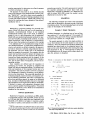
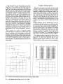
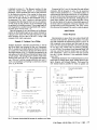
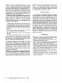
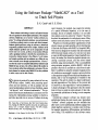
Using the Software Package "MathCAD" as a Tool
to Teach Soil Physics
D. K. Cassel* and D. E. Elrick
ABSTRACT
Many students avoid taking a course in soil physics because
they are apprehensive about higher mathematics. The computer
software, MathCAD, one of several "toolbox software programs" for solving mathematics problems, was used extensively
in teaching a graduate course on water and solute transport.
Students gained proficiency using the software as homework
assignments gradually became more complex. Students solved
simple arithmetic problems such as the computation of bulk
density and water content, problems of intermediate difficulty
such as graphing functions to describe the concentration of a
nonreactive chemical species in the effluent of a soil system,
and complex problems such as nonlinear curve fitting to construct a smooth curve through experimental data. A survey 7
mo after the course was completed indicated that students found
MathCAD easy to learn, the software allowed the student to
focus on physics rather than mathematics, and some of the students planned to continue using MathCAD to solve problems
in other courses and in their research.
S
on, PHYSICS is perceived by many students to be a very
difficult subject. Indeed, most practicing agronomists and soil scientists, as well as graduate and advanced undergraduate students in these disciplines, equate
"soil physics" with "advanced mathematics." This situation arises because mathematics is a necessary tool for
stating the relationships among variables to describe a
particular physical state or process. Problems involving
O.K. Cassel, Dep. of Soil Science, Box 7619, North Carolina State
Univ., Raleigh, NC 27695-7619; and D.E. Elrick, Dep. of Land Resource
Science, Univ. of Guelph, Guelph, Ontario, NIG 2W1, Canada.
Received 19 Mar. 1991. *Corresponding author.
Published in J. Nat. Resour. Life Sci. Educ. 21:74-78 (1992).
74
• J. Nat. Resour. Life Sci. Educ., Vol. 21, no. 1, 1992
water transport, for example, may require the solution
of a partial differential equation, or in the case of
drainage, the use of complex variables. It is our belief
that students worry less about the "physics" than they
do about the mathematics in a soil physics course. Many
students avoid soil physics courses for this very reason.
Progress in overcoming students' apprehension of soil
physics courses was made possible with the introduction
of the book Soil Physics with BASIC by Campbell (1985).
This book was designed for students who have mastered
differential and integral calculus, but who have not taken
a course in differential equations. Using Campbell's textbook, the student first learns the physical concepts concerning a particular process, and then solves related
problems using microcomputers. This is accomplished
using computer programs, coded in BASIC, which are
printed in the book or available on a disk from the publisher. In addition to using the computer program provided, students are encouraged to explore various solutions
to the equations using different initial and boundary conditions, and to vary the magnitudes of variables in the
equations. This activity results in a deeper understanding and appreciation of the physics of the process and
its sensitivity to the magnitudes of various parameters.
A major advantage of this approach is that the student
does not have to spend an undue amount of time making numerical calculations or having to write computer
programs.
Commercial computer software has become more
sophisticated during the past several years. Specialized
"toolbox" software programs are now available that
allow users to solve mathematical problems ranging from
simple algebraic operations to complex ones involving,
for example, integration, differentiation, and nonlinear
curve fitting. The availability of this software creates
another opportunity for instructors to refine the manner
in which soil physics is taught.
The purpose of this article is: (i) to briefly describe
someof the features of the mathematical software package "MathCAD"
~, and (ii) to show several examples
how this package was used in teaching a graduate course
in water and solute transport. MathCADsoftware was
selected for teaching the course because of the authors’
familiarity with it.
WHATIS MathCAD?
MathCADis a software package for personal computers. MathCAD
allows the user to write equations in
standard, two-dimensional format; to use standard
mathematical symbols; and to solve them. In addition,
graphs in two or three dimensions can be generated.
MathCAD
uses standard mathematical symbols for operators and variables, including Greek symbols. To create
simple expressions, such as addition or multiplication,
the user enters the numbers and operators (for example
+ for addition and * for multiplication) using the keys
on a standard keyboard. To create more complicated constructs, such as plots or definite integrals, the appropriate built-in function is selected using dedicated keys on
the keyboard. The user simply fills in the designated
blanks to complete the construct. For example, once the
proper key has been pressed to initiate the integral construct, the user must key in four entries to fill in the following four blanks associated with the integral: (i) the
expressionto be integrated, (ii) the upperlimit of integration, (iii) the lower limit of integration, and (iv) the
tegrating variable.
Once variables are defined and the equations or
constructs are written, the program is complete and
MathCAD
finds the numerical solution. The defined variables and equations of the program become part of a
"document" that can be printed or saved in a computer
file. Documents,in pieces or in entirety, can be imported into other documents. The numerical algorithms for
evaluating integrals, matrix inversion, and equation solving are standard, predictable, and robust. Commands
are
given from pull-down menus, by name or by dedicated
keys. An editor in MathCAD
allows the user to rearrange
the information on the screen and to add text and labels,
if desired, to create a self-explanatory documentwhen
sent to a printer capable of printing graphics. The printed
documentis identical in every detail to the information
displayed on the monitor.
monochromemonitor. No math coprocessor is required
but machine operations are much faster with one.
MathCADis licensed by MathSoft, Inc. MathCAD2.5
sells for about $180 (1991 price); the student version
(MathCAD2.0) sells for $40.
EXAMPLES
The following examples were used in the soil physics
course and are presented to illustrate several of the kinds
of problems solved. The accompanyingfigures are actual
copies of the display on the monitor.
Example1: Simple Calculation
Problem Statement: A cyfindrical core of wet soil having a radius of 3.7 cm and a height of 7.6 cm weighs 573
g and loses 110 g upon oven drying. Calculate bulk density and water content on a weight basis.
The easiest approach to solve this simple problem is
to use the keyboard in the same manner as one uses a
calculator. After the numbersand operators defining the
equation have been keyed in, the numerical answer appears on the screen immediately after entering the equal
sign (Approach A, Fig. 1). This approach is rapid, and
the information on the screen can be either saved in a
data file, printed, or discarded.
Problem
1: Calculation
A.
and
WATER
CONTENT
- 1.416
3.7’
3.7’
7.6
110
----= 0.238
573 - 110
B.
Second
approach:
Given information:
Mw := 110 g
Mass of Moll
Mt := 573 g
Total mass
r := 3.7 cm
Radius
of soil
core
L := 7.6 cm
Length
of soil
core
Volume
of soil
core
water
of wet soll
2
V :=
Db =
~ r L
Mt - MW
.......
V
-3
= 1.416
gcm
MW
Ow :
- 0.238
Mt - MW
8w =
~ The use of trade namesin this publication does not imply endorsementby the North Carolina Agric. Exp. Stn. or the University of Guelph
of the products named nor criticism of similar ones not mentioned.
DENSITY
573 - II0
Db -
Software Specifications
MathCAD
2.5 requires, at a minimum,an IBM, Apple,
or compatible computer with 512 RAM,at least one 5.25
or 3.50 inch disk drive (hard disks are supported), and
MS-DOS
or PC-DOS2.0 or higher. It requires a graphics printer or plotter, and operates on either a color or
of BULK
First approach:
- 23.758’%
Mt - MW
Fig. 1. Document
showingbulk density and water content calculations
and output using MathCAD.
J. Nat. Resour. Life Sci. Educ., Vol. 21, no. 1, 1992
Using ApproachB to solve this problem is more satisfying (Fig. 1). The "append" commandallows the user
to select one of three "scientific unit" files resident in
MathCAD.For example, appending the MKS(SI) unit
file allows the user to specify the units of each variable
in the equation in SI units. The answer is then automatically displayed in SI units. To begin solving this problem,
the numerical value for each symbol appearing in the
equations to follow is defined. Each equation is then written in terms of the previously defined symbols and, immediately upon keying in the equal sign for each
equation, its numerical answer and units are given. No
units exist for the computer water content because the
units cancel. By pressing the percent key after the unitless answer, the equation is automatically copied and the
answer given in percent. The equations are essentially
templates and can be used to solve the same problem
repeatedly (for different sets of input data) simply
changing the appropriate numerical value(s) of the variables defined in the "Given information" section in
Fig. 1.
This example was chosen to illustrate
several
MathCAD
features. In practice, it would be easier and
faster for a student to solve the problem on a hand-held
calculator. The following two examplesillustrate the types
of problems solved by graduate students using MathCAD
in an AdvancedSoil Physics class at the University of
Guelph during the 1990 spring semester. Noneof the students had previous experience using MathCAD
before the
course began.
Example2: Plotting Functions
Plotting the functional relationships between several
variables is a powerful learning tool because the student
can observe visually how a change in one or more independent variables affects the dependent variable. The
concept of the breakthrough or effluent concentration
curve is important in understanding solute transport in
soils (Van Genuchten and Wierenga, 1986). For this
problem the breakthrough curve is defined as the concentration of nonreacting solute flowing out of a soil system(e.g., out the base of a soil profile) plotted vs. p, the
numberof pore volumesof fluid flowing through the soil
system.
Problem Statement: Plot the breakthrough curves for
one-dimensional solute transport of a nonreacting chemical. The first solution, C1 (for brevity the equations are
not stated here, but are shownin Fig. 2) assumes an infinite soil column (Taylor, 1953). Solutions C2 (Lapidus
and Amundson, 1952) and C3 (Lindstrom et el., 1967)
assume first type (concentration) and third type (flux)
boundaryconditions, respectively, at the inlet end of a
semi-infinite soil column. For a comparisonof these and
other results, see Van Genuchten and Parker (1984).
The complete program to generate 25 pairs of numbers to plot the theoretical breakthrough curves for solutions C1, C2, and C3 are shown in Fig. 2. After
assigning the index variable i values for 1 to 25, the pore
volume variable p, which occurs in all three equations,
a := 5 B is theBrenner
or columnPeclet
number
o.~____~
: o.ooooo~
o.r~
, .9.oo62z
.,;;
|
o
Fig.
. . !
0
2. Document showing MathCADprogram and output
76 ¯ J. Nat.
Resour. Life
Sci.
Educ.,
Vol.
for
plotting
21, no. 1, 1992
complex functions.
C2
io
1.269814 10
0.000003
C3
io
2.727263
O.eO006
is defined in terms of i. The Brenner number, B, also
called the column Peclet number, is a dimensionless
parameter, which represents the ratio of the convective
to the dispersive processes. After typing the three equations as shown in Fig. 2, the "compute" commandis
given and the four columns of data displayed in Fig. 2
are generated. The "plot" function is activated with a
pre-assigned key allowing the three curves to be plotted.
A wide range of plot formats can be formulated using
the guidance of a pulldown menu. The average length of
time required by a student learning MathCAD
to generate these plots was less than l h.
Once the programis run, the influence of the Brenner
number on the breakthrough curves is easily obtained by
typing in a new value of B. The time required to run the
entire program for one value of B was 5 s using a 286
computer with math coprocessor.
Example3: Nonlinear Curve-Fitting
Problem Statement: Chloride concentration vs. time at
the 20-cm depth was obtained by Ian van Wesenbeeck
(Ph.D. student) at the Delhi Research Station in Ontario
on a sandy soil. (For brevity the data are shown only in
the output section of Fig. 3.) Chloride was applied to the
soil surface at the rate of 80 g of chloride per squaremeter
of soil surface. The average water content in the transmission zone was 0.30 mS/ms , the average bulk density
was 1.59 g/cm3, and the average infiltration rate was 3.5
cm/h. Use nonlinear curve fitting to construct a smooth
curve to fit the data.
Presented in Fig. 3 are: (A) the data files and defined
constants; (B) the program to solve for the numerical
values of three parameters (~r, /~, and MPA)subject
minimizing the least square mean error; (C) the computed values of the three fitting parameters; and (D) a plot
of the curve along with the input data. Althoughthe program looks complex, the user manual provides a stepby-step description of the process. Reasonableguesses of
the three unknownparameter values are required to begin the iterative curve-fitting process. The "plot" procedure discussed in Example2 was used to create the graph.
DISCUSSION
Student Response
Questionnaires to assess their views about MathCAD
were sent to all nine M.S. and Ph.D. students 7 moafter
they had completed the advanced soil physics course. In
their responses, seven students said they used the computer very often and one said often. Ona five-point scale
of very easy, easy, neither easy nor difficult, difficult,
or very difficult, five students found learning MathCAD
was easy, and three found it neither easy nor difficult.
One commented, "Once you know what the function
keys do, it is easy. However,it was somewhatfrustrating at first."
Additional statements were evaluated based on a fivepoint scale of strongly agree, agree, neither agree nor disagree, disagree, and strongly disagree. They agreed the
user manual made it possible for them to quickly use
Inputof experimental
Guessvalues
o :=.5
Thesearethebestguessvalues
of a,thevarianGe,
and~,themean,
Fig. 3. Documentshowing MathCAD
programfor nonlinear curve fitting.
d. Nat. Resour. Life Sci. Educ., Vol. 21, no. 1, 1992 ¯ 77
MathCAD. They also agreed the plot function was easy
to learn. They agreed using MathCAD made it possible
to focus on the physical properties of soils without spending too much time on the math. Comments included, "It
allowed me to look at the physics of the question without
having to review my calculus" and "The physics aspects
of soil properties and their mathematical descriptions are
supplementary to each other; therefore, without one the
other cannot be understood properly."
Students agreed that using MathCAD helped them clarify the functional relationships between variables. They
neither agreed nor disagreed with the statement,
"Without MathCAD, the course would have been
difficult because of the math." In their comments they
expanded on their responses:
"Although I have several university courses in calculus, my
working knowledge of math was not to the level that would
have made the physics course easy. MathCAD really helped."
"Although it helped in plotting analytical solutions and varying variables, it did not help with partial differential
equations."
"Difficult to say—perhaps I did not realize the amount of
time I would have spent without MathCAD."
"To understand MathCAD's output you must understand
the input."
They agreed they would continue to use MathCAD,
even if it were not an integral part of a course. Typical
statements were: "I'm using it to analyze my thesis data"
and "I'll continue to use MathCAD because it has a wide
range of math functions and operations."
In response to the question, "In general, how do you
think MathCAD helped you learn soil physics concepts
in this course?", one responded, "It helped me understand the relative importance/impact of changes in various input parameters on the output parameter, i.e., salt
concentration." Other responses indicated that
MathCAD had not hindered them in learning soil physics concepts in the course.
Balkovick et al. (1985) found that students have
difficulty translating an abstract mathematical formulation into an understanding of the phenomena that they
can use. Because of computational difficulty, faculty may
confine examples to problems that can be solved on the
78 • J. Nat. Resour. Life Sci. Educ., Vol. 21, no. 1, 1992
blackboard. This may limit assignments. With the computer, ".. .the students can be asked to pose a variety
of 'What if?' questions about problems so sufficiently
rich that not even the qualitative answers may be obvious" (Balkovick et al., 1985, p. 1215).
Instructor Response
We conclude that the various mathematical problemsolving procedures in MathCAD represent a powerful
tool for students as well as researchers to solve complicated problems. Advantages of using MathCAD in an advanced soil physics course include the following: (i)
relatively easy to learn to use, (ii) capable of solving complex equations, and (iii) relatively inexpensive. We are not
promoting the idea that MathCAD or any other computer
software package be substituted for learning mathematics. However, we do believe MathCAD and similar software greatly enhance the learning process by allowing
students (and faculty) to explore and experiment with
complex mathematical relationships in a time-efficient
manner. The favorable student response to MathCAD
supports our enthusiasm for using it as an aid to understanding soil physics.