Download ReaX: User Manual

ReaX: User Manual
Nicolas Berthier
April 30, 2015
ReaTK is the Reactive System Verification and Synthesis ToolKit. It provides the
ReaVer tool dedicated to the static verification of logico-numerical programs by
abstract interpretation, and the ReaX tool performing discrete controller synthesis
for such programs.
This manual details the ReaX tool by means of a small example and some explanations about its usage.
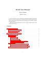
Contents
1 Installation Instructions
1.1 External Library Dependencies . . . . . . . . . . . . . . . . . . . . . . . . . . .
1.2 Installation using OPAM . . . . . . . . . . . . . . . . . . . . . . . . . . . . . .
1.3 Manual Compilation . . . . . . . . . . . . . . . . . . . . . . . . . . . . . . . . .
2
2
2
2
2 The Controllable-Nbac Language
2.1 Naming Conventions . . . . . . . . . . . . . . . . . . .
2.2 Global Structure . . . . . . . . . . . . . . . . . . . . . .
2.3 Common Rules . . . . . . . . . . . . . . . . . . . . . . .
2.3.1 Lexing Rules . . . . . . . . . . . . . . . . . . .
2.3.2 Expressions . . . . . . . . . . . . . . . . . . . .
2.3.3 Type-related Rules . . . . . . . . . . . . . . . .
2.3.4 Variable Declarations . . . . . . . . . . . . . . .
2.3.5 Local Variable Declaration and Definitions . . .
2.3.6 Declaring Weavable Signatures . . . . . . . . .
2.4 Main Entities . . . . . . . . . . . . . . . . . . . . . . . .
2.4.1 (Weavable) Node Specification (Ctrln/Ctrld) . .
2.4.2 (Weavable) Function Specification (Ctrlf) . . . .
2.4.3 (Weavable) Predicate Specification (Ctrlp/Ctrlr)
2.5 Variable Scope
TODO . .
2
2
3
3
3
3
4
4
4
5
6
6
6
6
7
1
.
.
.
.
.
.
.
.
.
.
.
.
.
.
.
.
.
.
.
.
.
.
.
.
.
.
.
.
.
.
.
.
.
.
.
.
.
.
.
.
.
.
.
.
.
.
.
.
.
.
.
.
.
.
.
.
.
.
.
.
.
.
.
.
.
.
.
.
.
.
.
.
.
.
.
.
.
.
.
.
.
.
.
.
.
.
.
.
.
.
.
.
.
.
.
.
.
.
.
.
.
.
.
.
.
.
.
.
.
.
.
.
.
.
.
.
.
.
.
.
.
.
.
.
.
.
.
.
.
.
.
.
.
.
.
.
.
.
.
.
.
.
.
.
.
.
.
.
.
.
.
.
.
.
.
.
.
.
.
.
.
.
.
.
.
.
.
.
.
.
.
.
.
.
.
.
.
.
.
.
.
.
3 Synthesizing using ReaX
3.1 Specifying a DCS Algorithm . . . . . . .
3.2 Available Synthesis Algorithms . . . . .
3.2.1 Common Flags . . . . . . . . . .
3.2.2 Boolean Synthesis (sB) . . . . . .
3.2.3 Approximating Synthesis (sS) . .
3.3 Available Abstract Domains . . . . . . .
3.4 Post-processing the Controller . . . . . .
3.4.1 One-step Optimization . . . . . .
3.4.2 Triangularization . . . . . . . . .
3.4.3 Triangularization & Merging . .
3.5 Example Executions . . . . . . . . . . . .
3.5.1 Finite-state Case . . . . . . . . .
3.5.2 Infinite-state Case . . . . . . . .
3.5.3 Synthesizing Towards Simulation
.
.
.
.
.
.
.
.
.
.
.
.
.
.
.
.
.
.
.
.
.
.
.
.
.
.
.
.
.
.
.
.
.
.
.
.
.
.
.
.
.
.
.
.
.
.
.
.
.
.
.
.
.
.
.
.
.
.
.
.
.
.
.
.
.
.
.
.
.
.
.
.
.
.
.
.
.
.
.
.
.
.
.
.
.
.
.
.
.
.
.
.
.
.
.
.
.
.
.
.
.
.
.
.
.
.
.
.
.
.
.
.
.
.
.
.
.
.
.
.
.
.
.
.
.
.
.
.
.
.
.
.
.
.
.
.
.
.
.
.
.
.
.
.
.
.
.
.
.
.
.
.
.
.
.
.
.
.
.
.
.
.
.
.
.
.
.
.
.
.
.
.
.
.
.
.
.
.
.
.
.
.
.
.
.
.
.
.
.
.
.
.
.
.
.
.
.
.
.
.
.
.
.
.
.
.
.
.
.
.
.
.
.
.
.
.
.
.
.
.
.
.
.
.
.
.
.
.
.
.
.
.
.
.
.
.
.
.
.
.
.
.
.
.
.
.
.
.
.
.
.
.
.
.
.
.
.
.
.
.
.
.
.
.
.
.
.
.
.
.
.
.
.
.
.
.
.
.
.
.
.
.
.
.
.
.
.
.
.
.
.
.
.
.
7
7
7
7
8
8
8
9
9
9
10
10
10
12
16
References
17
Index
18
1 Installation Instructions
1.1 External Library Dependencies
ReaTK and most of its dependencies are written using OCaml, yet some of its library dependencies require a decent version of GCC to be compiled, as well as development packages of
GMP and MPFR libraries (packages libgmp-dev and libmprf-dev under Debian-based
distributions, gmp-devel and mpfr-devel under Fedora).
1.2 Installation using OPAM
The recommended way for installing ReaTK is to use the OCaml Package Manager (OPAM).
See http://people.irisa.fr/Nicolas.Berthier/opam for further instructions.
1.3 Manual Compilation
Please refer to the README file at the root of the source tree.
2 The Controllable-Nbac Language
2.1 Naming Conventions
The tool ReaX handles input files that must define either a node, a function or a predicate.
By convention, file names of node, function and predicate should be suffixed with .ctrln,
.ctrlf and .ctrlp respectively. The file name extension .ctrld can be used for nodes
2
without controllable input variables (typically, for synthesis results), and .ctrlr can also
denote predicates.
2.2 Global Structure
Each of these types of inputs have a signature and a body. Signatures always define (name
and type) input variables; signature of nodes additionally specify state variables. The body is
essentially a set of assignments for state and/or output variables, possibly along with definitions
for local variables.
Controllable-Nbac files are divided into sections, each of which beginning with a keyword
starting with a ’!’.
2.3 Common Rules
Let’s first define basic lexing and grammar rules that are common to any category of input
understood by ReaX.
2.3.1 Lexing Rules
The Controllable-Nbac language is case-sensitive, and variables and type names are defined
classically as identifiers. Yet, one shall always start label names with an uppercase letter, and
variable names with any other allowed identifier character. Comments start with "(*", end with
"*)", and can be imbricated.
# Note all rules bellow are lexing ones: no space is allowed in between
# characters.
# Numbers
<digit> ::= '0' - '9'
<digits> ::= <digit> { <digit> }
<positive> ::= <digits>
<rational> ::= <digits> '/' <digits>
<real> ::= { <digit> } '.' <digits> [ ( 'e' | 'E' ) [ '+' | '-' ] <digits> ]
# Identifiers
<id> ::= <id-character> { <id-character> | <digit> | '!' }
<id-character> ::= 'A' - 'Z' | 'a' - 'z' | '_' | '@'
2.3.2 Expressions
Numerical constants are specified as usual, and the Boolean ones are true and false. Although
grammar rules do not impose any typing constraints on expressions, some type checking
is performed during parsing, and typing errors reported by ReaX may be interleaved with
syntax-related ones.
# Boolean constants
<bcst> ::= "true" | "false"
# Numerical constants
<ncst> ::= <positive> | <rational> | <real> | <bint>
<bint> ::= <bint-type> '(' [ '-' ] <positive> ')'
3
# Untyped expressions
<expr> ::= <bcst> | <ncst> | <id>
| <unary-operator> <expr>
| <expr> <binary-operator> <expr>
| "if" <expr> "then" <expr> "else" <expr>
| '#' '(' <exprs-list> ')'
| <ncst> <id>
| <expr> "in" '{' <exprs-list> '}'
| '(' <expr> ')'
<exprs-list> ::= <expr> { ',' <expr> }
# Available operators
<unary-operator> ::= "not" | '-'
<binary-operator> ::= "and" | "or" | "xor" | "eq" | '-' | '+' | '*' | '/'
| '<' | '>' | "<=" | ">=" | "<>" | '='
#(...) and in operators are syntactic sugar to encode respectively the mutual exclusion between
a list of Boolean expressions (i.e. at most one can hold at a time) and the membership test for
finite types. Semantics of the other constructs is straightforward.
2.3.3 Type-related Rules
An optional section for type specifications always comes first in Controllable-Nbac files.
# Type definition section
<typdefs> ::= "!typedef" { <typdecl> }
# Enuleration type declaration
<typdecl> ::= <id> '=' "enum" '{' <id> { ',' <id> } '}' ';'
# Type names
<type> ::= "bool" | "int" | "real" | <bint-type> | <id>
# Bounded integers
<bint-type> ::= ( "uint" | "sint" ) '[' <positive> ']'
2.3.4 Variable Declarations
Standard variable declarations are made using series of sets of identifiers, associated to their
type:
<var-decls> ::= <var-decls'> { <var-decls'> }
<var-decls'> ::= <id> { ',' <id> } ':' <type> ';'
2.3.5 Local Variable Declaration and Definitions
Every category of Controllable-Nbac input (node, function or predicate) may use local variables
to shorten or ease the specification of expressions. Local variables are declared and defined in
the !local and !definition sections:
# Declaration part
<local-decls> ::= "!local" <var-decls>
# Definition part
4
<local-defs> ::= "!definition" <local-def> { <local-def> }
<local-def> ::= <id> '=' <expr> ';'
A local variable transitively inherits the minimal scope among the variable dependencies of its
expression definition. See Section 2.5 for details about variable scopes.
2.3.6 Declaring Weavable Signatures
Non-controllable Variable Declarations A set of non-controllable variables must be declared within an !input section:
# Declaration of non-controllable variables
<input-decls> ::= "!input" <var-decls>
Controllable Variable Declarations The declaration of a sequence of controllable variables
takes place in !controllable sections, and additionally permits the specification of associated
default expressions:
# Declaration of controllable variables
<crtl-decls> ::= "!controllable" <ctrl-decls'> { <ctrl-decls'> }
<ctrl-decls'> ::= <ctrl-id> { ',' <ctrl-id> } ':' <type> ';'
<ctrl-id> ::= <id> [ '?' <expr> ]
U/C groups Specification
sections.
U/C groups are declared by alternating !input and !controllable
# Possibly empty sequence of U/C groups
<uc-groups-decl> ::= { <uc-group-decl> } [ <uc-group-final-u> ]
| <uc-group-only-c>
<uc-group-decl> ::= <input-decls> <ctrl-decls>
<uc-group-final-u> ::= <input-decls>
<uc-group-only-c> ::= <ctrl-decls>
U/C group sequences must start with the declaration of a set of non-controllable inputs, unless
all inputs are controllable.
I/O groups Specification I/O groups are the counterpart of U/C groups, and typically define
the signature of a function resulting from the triangularization of a controller synthesized for a
weavable node. I/O groups are declared by alternating !input and !output sections.
# Non-empty sequence of I/O groups
<io-groups-decl> ::= <io-group-decl> [ <io-group-final-i> ]
| <io-group-only-o>
<io-group-decl> ::= <io-group-decl'> { <io-group-decl'> }
<io-group-decl'> ::= <input-decls> <output-decls>
<io-group-final-i> ::= <input-decls>
<io-group-only-o> ::= <output-decls>
<output-decls> ::= "!output" <var-decls>
I/O group sequences must start with the declaration of a set of non-controllable inputs, unless
all inputs are controllable.
5
2.4 Main Entities
2.4.1 (Weavable) Node Specification (Ctrln/Ctrld)
A Controllable-Nbac node is specified as an input stream whose syntax is as defined by the
rule bellow:
<node>
# Main rule
<node> ::= [ <typdefs> ] <node-decls> <local-defs> <trans-func> <node-formulas>
# Variable declaration sections
<node-decls> ::= <state-decls> [ <uc-groups-decl> ] [ <local-decls> ]
<state-decls> ::= "!state" <var-decls>
# Node formulas definitions
<node-formulas> ::= { ( <assertion> | <initial> | <final>
| <invariant> | <reach> | <attract> ) ';' }
<assertion> ::= "!assertion" <expr>
<initial> ::= "!initial" <expr>
<final> ::= "!final" <expr>
<invariant> ::= "!invariant" <expr>
<reach> ::= "!reachable" <expr>
<attract> ::= "!attractive" <expr>
Note that zeroadic nodes (i.e. without any !input nor !controllable sections) are admitted.
Further, non-controllable nodes (Ctrld — i.e. without any !controllable section) are also valid.
Transition Function Definitions The transition function of nodes are specified as assignments of state variables according to the following syntax:
<trans-func> ::= "!transition" <assign> { <assign> }
<assign> ::= <id> ( ":=" | "'" '=' ) <expr> ';'
2.4.2 (Weavable) Function Specification (Ctrlf)
A Controllable-Nbac function defines output vectors based on inputs. Its grammar is as defined
by the <func> rule bellow:
# Main rule
<func> ::= [ <typdefs> ] <func-decls> <local-defs> <func-formulas>
# Variable declaration sections
<func-decls> ::= [ <io-groups-decl> ] [ <local-decls> ]
# Optional assertion on inputs & outputs
<func-formulas> ::= [ <assertion> ';' ]
Zeroadic functions (i.e. without any !input nor !output sections) are not admitted.
2.4.3 (Weavable) Predicate Specification (Ctrlp/Ctrlr)
A Controllable-Nbac predicate is a Boolean function without state. Its grammar is as defined by
the <pred> rule bellow:
# Main rule
<pred> ::= [ <typdefs> ] <pred-decls> <local-defs> <pred-def>
6
# Variable declaration sections
<pred-decls> ::= [ <uc-groups-decl> ] [ <local-decls> ]
# Predicate definition
<pred-def> ::= "!value" <expr> ';'
As for nodes, zeroadic predicates (i.e. without any
admitted.
!input
nor
!controllable
sections) are
2.5 Variable Scope
TODO
Where variables can be used, especially the local ones.
3 Synthesizing using ReaX
3.1 Specifying a DCS Algorithm
In order to compute a controller, one first needs to select one of the synthesis algorithms
available in ReaX, and optionally provide additional options for it. On the command line, the
algorithm descriptor can be specified as an string immediately following the -a (short version
of --algo) flag.
Algorithm-specific options can be set by appending a colon to the algorithm descriptor,
followed by a comma-separated list of option flags or assignments, and values for complex
options (e.g. lists of variables, abstract domain descriptors) must be enclosed in brackets. For
instance, Algo:flag,option1=42,option2={foo,bar} selects an algorithm Algo,
sets the a flag flag, an option option1 to value 42 and option2 to a list of two strings.
Flags are considered disabled by default.
3.2 Available Synthesis Algorithms
ReaX currently implements two synthesis algorithms: an exact (also referred to as “Boolean”)
and an approximating one. The former is dedicated to operate on finite state systems, and the
latter is capable of handling infinite ones.
3.2.1 Common Flags
Table 1 lists the flags that are common to all synthesis algorithms.
Table 1: Flags that are common to all synthesis algorithms.
deads Exclude initial deadlocking states from the invariant
nobnd Disable computation of boundary transitions in the controller
7
3.2.2 Boolean Synthesis (sB)
If the input node does not comprise any numerical state variable, then the exact synthesis
algorithm can be used to compute a controller. The descriptor for this algorithm is sB, and its
additional flags are given in Table 2. Note that !reachable and !attractive sections of the input
Table 2: Flags specific to the Boolean synthesis algorithm.
r Enable reachability property enforcement
a Enable attractivity property enforcement (may be buggy for now)
node are ignored by ReaX unless the corresponding flag is explicitly set.
Audacious Usage Notice that the Boolean synthesis algorithm may compute correct results
for nodes involving numerical components in their vector of state variables (even if these state
variables do not encode outputs — see Section "A Note on Specifying Outputs" of the Technical
References Manual). It may however never terminate and lead to an explosion of memory
consumption in this case.
3.2.3 Approximating Synthesis (sS)
In case the vector of state variables involves numerical variables, one should consider using
the approximating algorithm with abstract interpretation. To do so, one should use the sS
algorithm specifier. Available flags for this algorithm are listed in Table 3 and options are listed
in Table 4.
Table 3: Flags specific to the approximating synthesis algorithm.
split Perform the "split" algorithm for handling of non-convex set of
forbidden states (may lead to deadlocks in the result)
bdisj Force full DNF decomposition of forbidden states predicate when
using the "split" algorithm
Table 4: Options specific to the approximating synthesis algorithm.
d Abstract domain specification (cf Section 3.3 below)
ws Maximum number of ascending iterations before resorting to base
widening
wd Number of descending iterations after base widening
3.3 Available Abstract Domains
Abstract domains are specified in a way similar to synthesis algorithms, and all share a common
set of options. The first component of abstract domains is the numerical abstraction, that can
be specified using one selector of Table 5. After having chosen the numerical domain, several
8
flags and options are available, that are listed in Table 6. Table 7 lists additional options for the
convex polyhedra numerical abstract domain.
I
O
P
b/m
s/l
Table 5: Numerical abstract domain selectors.
Intervals (Boxes)
Octagons
Convex Polyhedra
Table 6: Options for abstract domain composition.
Select BDD-based / MTBDD-based composition (default is BDDbased); MTBDD-based is generally less efficient, yet it might perform
better for disjunctive domains
Table 7: Convex polyhedra options.
Select Strict / Loose convex polyhedra
3.4 Post-processing the Controller
A successful synthesis produces a controller (Ctrlr) in the form of a predicate over the signature
of the initial node (state variables plus inputs). As noted in Section "Synthesis Product(s)" of
the Technical References Manual, this predicate is non-deterministic. Several possibilities exist
to reduce this non-determinism, and even to make a function (i.e. executable code) out of it.
Computation steps performed on controllers computed using one of the DCS algorithms above
are called post-processing steps.
3.4.1 One-step Optimization
One-step optimization can be used to reduce the level of non-determinism of the controller by
restricting its possible choices according to given criteria. For instance, a controlled system
whose controller has undergone one-step minimization of a state variable x will always enter
one of the immediate successor states for which the value of x is the smallest.
ReaX implements one-step minimization and maximization of numerical state variables, that
can be triggered by using the -O command line flag followed by an optimization specification of
the form “o1:<specs>”, where <specs> is a sequence (expressing priority) of goals that are
listed in Table 8. See Section Exemplifying One-step Minimization on page 17 for an example
usage of this feature.
3.4.2 Triangularization
ReaX is able to triangularize the controller using the default expressions for controllable inputs, to produce a function as detailed in Section Section “Triangularization Procedure” of the
9
min v
max v
Table 8: One-step optimization goals available.
Minimization of numerical state variable v
Maximization of numerical state variable v
Technical References Manual. Triangularization of the controller is performed when the -t
(or --triang) flag is given on the command line. In this case, a Controllable-Nbac function is
produced (Ctrlf).
3.4.3 Triangularization & Merging
Additional post-processing can be carried out when the -m (or --merge) flag is given (this
flag forces triangularization). In such a case, the controllable inputs involved in the transition
function of the original node are substituted with the corresponding equation resulting from the
triangularization. The output of ReaX then becomes a classical (non-controllable) node (Ctrld).
3.5 Example Executions
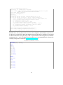
3.5.1 Finite-state Case
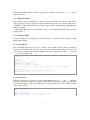
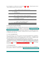
Example Controllable-Nbac Node Let the file 2tasks.ctrln exclusively contain the
Controllable-Nbac code as listed bellow. It describes a node (almost) equivalent to the one
described as Figure 3 in the paper introducting ReaX (Berthier and Marchand, 2014). In terms
of behavior, the main difference lies in the ability of the controller to force entering Idle from
Active. Its automaton representation is shown in Figure 1.
r∧c
¬(r ∧ c)
Idle
Active
s∨c
Figure 1: Task automaton.
2tasks.ctrln
!typedef
S = enum {Idle, Active};
!state
t1, t2: S;
!input
r1, r2, s1, s2, _c1: bool;
!controllable
c1 ? _c1, c2 ? c1: bool;
!transition
t1' = if t1 = Idle
and r1 and c1
then Active else
10
¬(s ∨ c)
if t1 = Active and (s1 or c1) then Idle
else t1;
t2' = if t2 = Idle
and r2 and c2 then Active else
if t2 = Active and (s2 or c2) then Idle
else t2;
!initial
t1 = Idle and t2 = Idle;
!invariant
#(t1 = Active, t2 = Active);
Remark that in this example, the default value for controllable input c1 is specified as additional
non-controllable input _c1; for illustrative purpose, the default value of c2 is the effective value
of c1 (to be chosen by the controller).
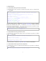
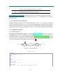
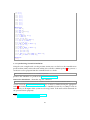
Executing ReaX for Boolean Synthesis To compute a controller for this node using the
Boolean synthesis algorithm (sB), to triangularize it (-t), and also to show basic debugging
information about the execution of ReaX (--debug D), one can use the following command
line:
reax 2tasks.ctrln -a 'sB' -t --debug D
The program reports on its execution using a sequence of log entries as listed bellow. Each
log entry starts with a measure of the time it effectively used the processor since the beginning
of its execution (in seconds). Following are a character describing the log level: ’E’ for errors, ’W’
for warnings, ’I’ for general information (the default level), and ’D’, ’d’ and ’.’ for three further
debugging levels. Then comes the name of an internal module of ReaX and the payload itself.
[0.029 I Main] Reading node from ‘2tasks.ctrln’...
[0.051 I Supra] Variables(bool/num): state=(2/0), i=(7/0), u=(5/0), c=(2/0)
[0.052 I Df2cf] Preprocessing: discrete program
[0.052 I Synth] Boolean synthesis:
[0.052 D sB] ++ ϕ = t1 = Idle or t1 = Active and t2 = Idle (= ~β)
[0.052 I sB] ++> Invariance:
[0.052 I sB] ++<
[0.052 D sB] β = t1 = Active and t2 = Active
[0.053 I sB] I∩β=∅ = true (= success)
[0.053 I sB] Building controller...
[0.053 I sB] Computing boundary transtions...
[0.053 I sB] Simplifying controller...
[0.053 I Synth] Boolean synthesis succeeded.
[0.055 I Env] CUDD reordering...
[0.063 I t.] Triangulation...
[0.063 D t.]
- U/C group 1:
c1’ = _c1;
c2’ = c1 and not r1
or c1 and r1 and not r2 and t1 = Idle
or c1 and r1 and r2 and t1 = Idle and t2 = Active
or c1 and r1 and t1 = Active;
[0.064 I Main] Extracting triangularized controller...
[0.064 I Main] Checking triangularized controller...
[0.065 I Main] Outputting into ‘2tasks.ctrlf’...
The resulting output file file:2tasks.ctrlf encodes the triangulated controller. Observe that its
inputs are the union of all state and non-controllable inputs of the original node, and its outputs
are the two controllable inputs.
11
2tasks.ctrlf
!typedef
S = enum {Idle, Active};
!input
t1: S;
t2: S;
r1: bool;
r2: bool;
s1: bool;
s2: bool;
_c1: bool;
!output
c1: bool;
c2: bool;
!local
l0: bool;
l1: bool;
l2: bool;
l3: bool;
l4: bool;
l5: bool;
!definition
c1 = _c1;
l0 = not r1;
l1 = not r2;
l2 = (t2 = Active);
l3 = (l1 or l2);
l4 = ((t1 = Active) or l3);
l5 = (l0 or l4);
c2 = c1 and l5;
!assertion
true;
3.5.2 Infinite-state Case
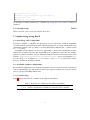
Example Node Consider an extended version of the previous example finite ControllableNbac node, now involving a numerical state variable. In this model, additional state variables x1
and x2 are used to count the number of steps spent in the Active state for each task.
Let 2tasks-counters.ctrln be the file:
2tasks-counters.ctrln
!typedef
S = enum {Idle, Active};
!state
t1, t2: S;
x1, x2: int;
!input
r1, r2, s1, s2, _c1, _c2: bool;
!controllable
c1 ? _c1, c2 ? _c2: bool;
12
!transition
t1' = if t1
if t1
x1' = if t1
if t1
t2' = if t2
if t2
x2' = if t2
if t2
=
=
=
=
=
=
=
=
Idle
Active
Idle
Active
Idle
Active
Idle
Active
and r1 and c1 then Active
and (s1 or c1) then Idle
and r1 and c1 then 0
then x1 + 1
and r2 and c2 then Active
and (s2 or c2) then Idle
and r2 and c2 then 0
then x2 + 1
else
else
else
else
else
else
else
else
t1;
x1;
t2;
x2;
!initial
t1 = Idle and t2 = Idle and x1 = 0 and x2 = 0;
!invariant
#(t1 = Active, t2 = Active) and x1 <= 10 and x2 <= 10;
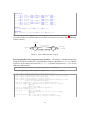
It encodes the parallel composition of two instances of the automaton of Figure 2. Here, the
invariant to enforce is both the mutual exclusion between the Active states, and the bounding
of their counters.
x := 0
r ∧ c/x := 0
¬(r ∧ c)
Idle
Active
¬(s ∨ c)/
x := x + 1
s ∨ c/x := x + 1
Figure 2: Task automaton with counter.
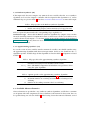
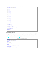
Executing ReaX for Over-approximating Synthesis To compute a controller for this node
using the deadlock-avoiding over-approximating synthesis algorithm (sS:deads) with the
disjunctive power domain over intervals (d={I:D}), and then triangularize it (-t), we use the
following command line:
reax 2tasks-counters.ctrln -a 'sS:d={I:D},deads' -t --debug D2
The corresponding rather detailed execution trace (--debug D2) shows:
[0.023
[0.046
[0.046
[0.046
[0.047
I
I
I
I
I
[0.047 D
[0.048 d
[0.049 d
[0.049 d
[0.049 d
[0.055 d
Main] Reading node from ‘2tasks-counters.ctrln’...
Supra] Variables(bool/num): state=(2/2), i=(8/0), u=(6/0), c=(2/0)
Df2cf] Preprocessing: discrete program
Verif] Forcing selection of power domain.
Synth] logico-numerical synthesis with powerset extension of power
domain over intervals with BDDs:
s.] Computing the original set of deadlocking states.
sS] α(F) = {Jt1 = Active and t2 = Active 7→ x1610 ∧ x2610K,
Jx2>11K,
Jx1>11 ∧ x2610K}
s.] Beginning of least fixpoint computation.
sS] Traversing arc 1.
sS]
B = {Jx1>11 ∧ x2610K,
Jt1 = Active and t2 = Active 7→ x1610 ∧ x2610K,
Jx2>11K}
sS] pre^ = {Jt1 = Idle and t2 = Active 7→ x2>10K,
Jt1 = Idle and t2 = Active 7→ x1>11 ∧ x269K,
13
[0.057 d sS]
[0.057 d sS]
[0.066 d sS]
[0.069 d sS]
[0.069 d sS]
[0.078 d sS]
[0.081 d s.]
[0.082 d s.]
[0.083 d s.]
[0.083 D sS]
[0.085 d s.]
[0.086 I sB]
[0.087 I sB]
Jt1 = Active and t2 = Idle 7→ x2>11K,
Jt1 = Active and t2 = Idle 7→ x1>10 ∧ x2610K,
Jt1 = Idle and t2 = Idle 7→ x2>11K,
Jt1 = Active and t2 = Active 7→ x1>10 ∧ x269K,
Jt1 = Idle and t2 = Idle 7→ x1>11 ∧ x2610K,
Jt1 = Active and t2 = Active 7→ x2>10K}
Traversing arc 1.
B = {Jt1 = Active and t2 = Active 7→ x2>10K,
Jx2>11K,
Jt1 = Active and t2 = Idle 7→ x1>10 ∧ x2610K,
Jt1 = Active and t2 = Active 7→ x1610 ∧ x2610K,
Jt1 = Idle and t2 = Active 7→ x2>10K,
Jt1 = Active and t2 = Active 7→ x1>10 ∧ x269K,
Jx1>11 ∧ x2610K}
pre^ = {Jt1 = Idle and t2 = Active 7→ x2>10K,
Jt1 = Idle and t2 = Active 7→ x1>11 ∧ x269K,
Jt1 = Active and t2 = Idle 7→ x2>11K,
Jt1 = Active and t2 = Idle 7→ x1>10 ∧ x2610K,
Jt1 = Idle and t2 = Idle 7→ x2>11K,
Jt1 = Active and t2 = Active 7→ x1>10 ∧ x269K,
Jt1 = Idle and t2 = Idle 7→ x1>11 ∧ x2610K,
Jt1 = Active and t2 = Active 7→ x2>10K}
Traversing arc 1.
B = {Jt1 = Active and t2 = Active 7→ x2>10K,
Jx2>11K,
Jt1 = Active and t2 = Idle 7→ x1>10 ∧ x2610K,
Jt1 = Active and t2 = Active 7→ x1610 ∧ x2610K,
Jt1 = Idle and t2 = Active 7→ x2>10K,
Jt1 = Active and t2 = Active 7→ x1>10 ∧ x269K,
Jx1>11 ∧ x2610K}
pre^ = {Jt1 = Idle and t2 = Active 7→ x1>11 ∧ x269K,
Jt1 = Idle and t2 = Idle 7→ x2>11K,
Jt1 = Active and t2 = Active 7→ x1>10 ∧ x269K,
Jt1 = Active and t2 = Idle 7→ x1>10 ∧ x2610K,
Jt1 = Idle and t2 = Idle 7→ x1>11 ∧ x2610K,
Jt1 = Active and t2 = Active 7→ x2>10K,
Jt1 = Idle and t2 = Active 7→ x2>10K,
Jt1 = Active and t2 = Idle 7→ x2>11K}
End of least fixpoint computation.
α(.-1) = {Jx2>11K,
Jx1>11 ∧ x2610K,
Jt1 = Idle and t2 = Active 7→ x2>10K,
Jt1 = Active and t2 = Active 7→ x1>10 ∧ x269K,
Jt1 = Active and t2 = Idle 7→ x1>10 ∧ x2610K,
Jt1 = Active and t2 = Active 7→ x2>10K,
Jt1 = Active and t2 = Active 7→ x1610 ∧ x2610K}
^u.I = ⊥
I(F) = {Jt1 = Active and t2 = Active 7→ x1610 ∧ x2610K,
Jt1 = Active and t2 = Idle 7→ x1>10 ∧ x2610K,
Jt1 = Idle and t2 = Active 7→ x2>10K,
Jx2>11K,
Jx1>11 ∧ x2610K,
Jt1 = Active and t2 = Active 7→ x1>10 ∧ x269K,
Jt1 = Active and t2 = Active 7→ x2>10K}
~γ(^) = t1 = Idle and t2 = Idle and -x2+10>=0 and -x1+10>=0
or t1 = Idle and t2 = Active and -x2+10>=0 and -x1+10>=0
and -x2+9>=0
or t1 = Active and t2 = Idle and -x2+10>=0 and -x1+10>=0
and -x1+9>=0
(= G)
Building controller...
Computing boundary transtions...
14
[0.087 I sB] Simplifying controller...
[0.087 d sB]
K = (43n,177m) (= <G>∩A∩G)
[0.087 I Synth] logico-numerical synthesis with powerset extension of power
domain over intervals with BDDs succeeded.
[0.089 I Env] CUDD reordering...
[0.102 I t.] Triangulation...
[0.102 D t.]
- U/C group 1:
c1’ = not _c1 and not s1 and t1 = Active and x1-9>=0 or _c1;
c2’ = not _c2 and not r1 and not s2 and t2 = Active and x2-9>=0
or not _c2 and not c1 and r1 and not s2 and t2 = Active and x2-9>=0
or not _c2 and c1 and r1 and not s2 and t2 = Active
or _c2 and not r1 and t1 = Idle
or _c2 and not c1 and r1 and t1 = Idle
or _c2 and c1 and r1 and not r2 and t1 = Idle
or _c2 and c1 and r1 and r2 and t1 = Idle and t2 = Active
or _c2 and not c1 and not r2 and not s1 and t1 = Active
or _c2 and c1 and not s1 and t1 = Active
or _c2 and s1 and t1 = Active;
[0.104 I Main] Extracting triangularized controller...
[0.105 I Main] Checking triangularized controller...
[0.107 I Main] Outputting into ‘2tasks-counters.ctrlf’...
From this trace, one can observe the successive values computed, and notably the set of states to
be effectively avoided (I(F)). Note that the BDD representation of the controller (K) is printed
in abbreviated form as it is quite large; still, a representation of the triangularized controller
(assignments of c1 and c2) is shown at the end of the trace. In Controllable-Nbac format, the
resulting triangularized controller file:2tasks-counters.ctrlf is:
2tasks-counters.ctrlf
!typedef
S = enum {Idle, Active};
!input
t1: S;
t2: S;
x1: int;
x2: int;
r1: bool;
r2: bool;
s1: bool;
s2: bool;
_c1: bool;
_c2: bool;
!output
c1: bool;
c2: bool;
!local
l0: bool;
l1: bool;
l2: bool;
l3: bool;
l4: bool;
l5: bool;
l6: bool;
l7: bool;
15
l8: bool;
l9: bool;
l10: bool;
l11: bool;
l12: bool;
l13: bool;
l14: bool;
l15: bool;
l16: bool;
l17: bool;
!definition
l0 = not s1;
l3 = not s2;
l4 = (t2 = Active);
l9 = not r2;
l12 = not r1;
l1 = l0 and (x1 >= 9);
l5 = l3 and l4;
l14 = (l9 or l4);
l2 = (t1 = Active) and l1;
l6 = (x2 >= 9) and l5;
c1 = (_c1 or l2);
l7 = (if c1 then l5 else l6);
l10 = (c1 or l9);
l13 = not c1;
l8 = (if r1 then l7 else l6);
l11 = (s1 or l10);
l15 = (l13 or l14);
l16 = (l12 or l15);
l17 = (if (t1 = Idle) then l16 else l11);
c2 = (if _c2 then l17 else l8);
!assertion
true;
3.5.3 Synthesizing Towards Simulation
Using the same example node as in the previous Section, one can also leave the controller in its
predicate form (Ctrlr), and use the tool ctrl2lut (also available as OPAM package1 ) to generate a
stochastic reactive program from the controlled node as a whole:
reax 2tasks-counters.ctrln -a 'sS:d={I:D},deads'
produces the controller as a predicate in file:2tasks-counters.ctrlr.
Interactive Simulation
From this step, the command
ctrl2lut -o two-tasks-counters.lut 2tasks-counters.ctrln 2tasks-counters.ctrlr
creates a Lutin file file:two-tasks-counters.lut, that can then be simulated using the appropriate
tools2 . For instance, one can simulate the above controlled system by executing Luciole to
interactively set all inputs of the system at each step (“main” is the name of the main node in
the generated Lutin program):
1
2
See http://people.irisa.fr/Nicolas.Berthier/opam#ctrl2lut.
See http://www-verimag.imag.fr/Lutin.html.
16
lutin -n main -luciole two-tasks-counters.lut
Although Lutin does not support non-Boolean finite variables (i.e. enumerations) for now,
ctrl2lut is able to handle them: it one-hot encodes such variables to keep the input and output
signals readable. Note however that finite numerical variables are not supported.
Automated Simulation Alternatively, one can also use the ctrl2lut tool to generate a stochastic environment node generating the inputs of the controller (or original) node from the values
of its state variables, and by ensuring that its assertion is not violated.
ctrl2lut -o two-tasks-counters.lut 2tasks-counters.ctrln 2tasks-counters.ctrlr \
-e -eo two-tasks-counters-env.lut
In this case, the simulation can be launched using Lurette3 :
lurettetop \
-rp 'sut:lutin:two-tasks-counters.lut:main' \
-rp 'env:lutin:two-tasks-counters-env.lut:env'
Exemplifying One-step Minimization To perform one-step optimization targeting the
minimization of x1 and then of x2, one can use:
reax 2tasks-counters.ctrln -a 'sS:d={I:D},deads' -O 'o1:min x1,min x2'
References
Berthier, N. and Marchand, H. (2014). Discrete controller synthesis for infinite state systems
with ReaX. In 12th Int. Workshop on Discrete Event Systems, WODES ’14.
3
See http://www-verimag.imag.fr/Lurette,107.html.
17
Index
abstract domain, 8
controllable variable, 5
Controllable-Nbac
function, 6
I/O group, 5
keyword
enum, 4
in, 4
node, 6
predicate, 6
section
assertion, 6
attractive, 6
controllable, 5
definition, 4
final, 6
initial, 6
input, 5
invariant, 6
local, 4
output, 5
reachable, 6
state, 6
transition, 6
typedef, 4
value, 6
U/C group, 5
default expression, 5
synthesis algorithm, 7
approximating, 8
Boolean, 8
18