Download Athlete DSS and data analysis

POLITECNICO DI TORINO
III Facoltà di Ingegneria
Corso di Laurea in Ingegneria Informatica
Tesi di Laurea Magistrale
Athlete DSS and data analysis
Relatore:
Prof. Pau F ONSECA I C ASAS
Candidato:
Gianfranco A RCAI
Gennaio 2008
II
Sommario
Il lavoro che viene presentato si pone l’obiettivo di illustrare in dettaglio l’attività svolta durante il periodo di tesi presso la UPC (Universitat Politècnica de Catalunya) ed
analizzare gli aspetti teorici che la supportano.
Il lavoro di tesi riguarda la collaborazione allo sviluppo del progetto denominato
+Atleta. Lo scopo di tale progetto è quello di realizzare un DSS (Decision Support System) in ambito sportivo; tale software avrà la funzione di monitorare le prestazioni di
un elevato numero di atleti fornendo l’analisi approfondita dei dati, al fine di perseguire
il miglioramento del rendimento sportivo degli atleti stessi. Partendo dall’analisi dei parametri biologici, il software sarà inoltre in grado di simulare le prestazioni future degli
atleti.
Il lavoro svolto è stato incentrato sullo sviluppo del progetto esistente e sull’aggiunta
di nuove funzionalità al programma. Il progetto +Atleta, che prese il via nel 2005, si trova
nella fase di ultimazione dell’intera infrastruttura del sistema, grazie alla quale si potranno
eseguire in futuro le simulazioni di prestazioni. Per raggiungere questo obiettivo, devono
essere presi in considerazione numerosi fattori: i parametri biologici dell’atleta, i dati
relativi ad ogni gara od allenamento, le condizioni meteorologiche e quelle ambientali.
Scendendo nel dettaglio, sono stati studiati ed implementati algoritmi di analisi dei
dati relativamente allo sforzo fisico dell’atleta, al profilo altimetrico della corsa ed alle
caratteristiche topografiche del percorso di gara. Ciò ha determinato la creazione di numerose viste statistiche (suddivise per categoria) e l’analisi di alcuni fattori mediante la
regressione lineare. Il lavoro è iniziato con lo studio del sistema preesistente e, passando
attraverso lo studio della struttura di analisi dei dati, si è concluso con l’implementazione
III
delle nuove funzionalità. Nel presente documento saranno pertanto descritti gli obiettivi,
le scelte progettuali e le implementazioni realizzate durante il periodo di lavoro di tesi. Al
termine verranno riportate le conclusioni con relative considerazioni finali.
1.1
Introduzione
Attualmente, nel mondo dello sport, la competitività a livello professionistico è talmente
alta che si ricerca l’aiuto di qualsiasi strumento per migliorare le prestazioni ed il rendimento di un atleta. Negli ultimi anni, si fa sempre più ricorso alla tecnologia, in quanto
ci si è resi conto che il suo impiego nelle diverse discipline sportive ha avuto come conseguenza il miglioramento dei risultati ottenuti in precedenza. Si è arrivati al punto, a
livello professionistico, che un qualsivoglia margine di miglioramento, per quanto piccolo possa essere, possa tramutarsi nel superamento dell’attuale record mondiale oppure,
più semplicemente, in una vittoria.
L’uomo, per sua natura, è molto competitivo e tende a migliorarsi ed a superare se
stesso ed i propri limiti, giorno dopo giorno. Per raggiungere questo obiettivo è obbligato
a tenere sempre sotto osservazione quei parametri che lo portano a incrementare le proprie
prestazioni, in modo da poter lavorare sempre con la massima efficienza. Per questo
motivo, esiste oggi un gran numero di aziende, spesso multinazionali, che già da anni
puntano molto su progetti di questo tipo. Lo spettro delle possibili attività è piuttosto
ampio e variegato: alcuni produttori si occupano della strumentazione professionale in
grado di rilevare i parametri biologici dell’atleta, certe aziende offrono servizi di analisi
dei dati raccolti come supporto alle decisioni in merito allo stato fisico di un soggetto,
altre aziende ancora si preoccupano di produrre l’abbigliamento sportivo più adatto alla
disciplina praticata. Oltre a ciò, si è assistito alla istituzione di numerosi centri sportivi
specializzati in questo campo, di norma al servizio di società sportive di grande rilievo,
nei quali viene impiegata tecnologia all’avanguardia e personale altamente qualificato per
perseguire lo scopo del miglioramento delle prestazioni sportive degli atleti.
All’interno di questo complesso scenario è nato presso la UPC (Universitat Politècnica
IV
de Catalunya) di Barcellona il progetto denominato +Atleta. Tale progetto, curato dal Professor Pau Fonseca i Casas, si colloca nell’ambito dell’analisi dei dati sportivi. +Atleta
è stato ideato a seguito di una lunga ed approfondita analisi relativamente ai prodotti esistenti sul mercato. Detta ricerca ne ha preso in esame le caratteristiche, i punti forti e quelli
deboli, al fine di evidenziarne i limiti, le carenze e tutte le future possibilità di sviluppo.
Sono stati presi come modello per l’analisi le aziende leader in questo settore; in particolare si tratta di tre aziende di rilievo internazionale: POLAR, GARMIN e SUUNTO. Tali
imprese producono pulsometri professionali e forniscono al cliente software proprietari
che, una volta installati sul proprio PC, provvedono a visualizzare e gestire i dati raccolti
durante una gara od una qualsiasi sessione di allenamento. I parametri biologici raccolti,
non subiscono tuttavia profonde analisi, ma nella maggior parte dei casi vengono solamente mostrati all’utente sotto forma di grafico o di tabella. Ciò significa che, rispetto
alle informazioni che il pulsometro stesso fornisce in tempo reale durante il periodo di
attività fisica, il software non introduce sostanziali novità, se non quella di mostrare i dati
in forma più leggibile. Inoltre, l’utente deve necessariamente utilizzare il software fornito dalla ditta costruttrice dell’apparecchio che ha acquistato, poiché ciascuna impresa
utilizza un formato di dati proprietario. Questo fattore costituisce uno svantaggio non
indifferente, poiché con lo stesso programma non è possibile visualizzare dati provenienti
da strumenti di marche distinte.
A seguito di tali considerazioni, si inserisce l’idea di creare uno strumento nuovo,
nato dall’esigenza di ovviare alle carenze di quelli esistenti, per superarne le limitazioni
e proporsi come alternativa, in particolar modo per quanto riguarda l’uso professionale.
Il progetto +Atleta si propone dunque come strumento in grado di offrire caratteristiche e
funzionalità nuove nel settore dell’analisi dei dati biologici. Esso prese il via nel settembre
del 2005 e si trova tuttora in fase di sviluppo. Tale progetto, di durata pluriennale, ha
come obiettivo quello di creare un DSS (Decision Support System), un software molto
complesso, in grado di permettere il monitoraggio costante e dettagliato delle prestazioni
sportive di un elevato numero di atleti e l’analisi approfondita dei dati raccolti, al fine di
perseguire il miglioramento del rendimento sportivo degli atleti stessi. Attraverso l’analisi
V
di una grande quantità di dati, il DSS si comporterà come un vero e proprio sistema di simulazione, con l’obiettivo di prevedere in anticipo le prestazioni future di un atleta in una
particolare disciplina, su uno specifico tracciato, con particolari condizioni atmosferiche
ed ambientali.
+Atleta si propone di creare un prodotto nuovo rispetto a quelli oggigiorno in commercio. Le carenze dei prodotti presenti sul mercato divengono dunque i punti di forza
di questo progetto. Facendo uso dei pulsometri delle già citate case costruttrici, il software +Atleta è concepito per essere uno strumento standard, in grado cioè di acquisire
ed elaborare dati provenienti da qualsivoglia strumento, indipendentemente dalla marca
o dal modello di quest’ultimo. I dati raccolti vengono tradotti e mappati in un file in
formato standard XML (si veda il paragrafo 2.4.3) e successivamente salvati in un database MySQL. Da un lato i dati vengono visualizzati all’utente sotto forma di grafico o
di tabella, in maniera tale da far risaltare quelli più importanti e significativi; dall’altro
subiscono elaborazioni più complesse al fine di calcolare numerosi parametri biologici
utili per monitorare e migliorare delicati aspetti della preparazione atletica. Tali parametri
biologici, ricavati da calcoli effettuati sui dati originari in ingresso, rappresentano fattori e
variabili che verranno immessi come input nel DSS ed andranno dunque ad incidere nella
simulazione delle prestazioni di un atleta.
La presente Tesi di laurea si occupa di descrivere il lavoro di collaborazione ed il ruolo assunto dal sottoscritto nello sviluppo del progetto +Atleta. Per volgere al termine, il
progetto +Atleta prevede il completamento di numerose ed elaborate fasi di lavoro; esse
sono state descritte nel paragrafo 2.1 (Project planning) e sono state pianificate in maniera
tale da poter essere svolte da più studenti contemporaneamente. Una fase propedeutica
del lavoro di tesi è stata dedicata allo studio dell’architettura, del funzionamento e della
direzione degli sviluppi relativi al il progetto esistente. Lo spettro delle attività da svolgere è piuttosto complesso, tanto da coinvolgere studenti con formazioni universitarie e
competenze diverse dall’ingegneria. L’attività svolta si colloca nella fase di ultimazione
dell’infrastruttura del sistema esistente, illustrato in ogni sua parte nel capitolo 2. Nello
svolgimento del lavoro sono state affrontate due principali tematiche: la prima consiste
VI
nella creazione della struttura atta ad effettuare l’analisi statistica dei dati mediante l’interfacciamento con il software R; previa una fase di studio del funzionamento e delle potenzialità del software R, l’attenzione è stata rivolta all’implementazione della regressione
lineare, analisi statistica che offre interessanti informazioni sullo stato fisico dell’atleta.
Tuttavia lo scopo principale di questo lavoro è stato quello di documentare la creazione
della struttura, descrivere i procedimenti ed i meccanismi del collegamento tra +Atleta
ed il software statistico, affinché ricercatori futuri, in possesso di buone competenze di
medicina sportiva, possano utilizzarla per analisi mirate, più efficienti e più complesse.
Il lavoro relativamente a questa parte è descritto nel capitolo 3. La seconda tematica affrontata riguarda invece l’ideazione di tre algoritmi di analisi di dati relativamente allo
sforzo fisico dell’atleta, al profilo altimetrico del percorso di gara ed alla planimetria della
corsa. Tali algoritmi hanno lo scopo di visualizzare statistiche relative al proprio ambito
e calcolare alcuni parametri che, come predetto, potranno essere utilizzati come input per
il simulatore. La teoria ed il funzionamento di tali algoritmi è dettagliatamente illustrata
nel capitolo 4. La parte successiva, affrontata nel capitolo 5 della Tesi, riguarda l’implementazione vera e propria di tali algoritmi mediante l’utilizzo dell’ambiente di sviluppo
c e del linguaggio di programmazione Visual C++.
Visual Studio 2005 della Microsoft Inoltre, si è realizzata un’adeguata interfaccia utente attraverso la quale è possibile disporre agevolmente di tutte le funzionalità aggiunte al software +Atleta. Sono esposte infine le
caratteristiche, le scelte progettuali effettuate, l’organizzazione delle classi implementate,
i diagrammi dei casi d’uso ed i diagrammi di sequenza propri del progetto di ingegneria
del software. L’ultimo capitolo (6) riporta le conclusioni sul lavoro svolto, la descrizione
dello stato attuale del progetto e le ipotesi sugli sviluppi futuri.
VII
1.2
Descrizione del sistema esistente
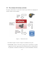
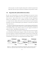
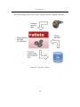
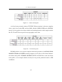
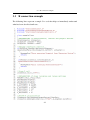
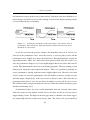
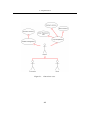
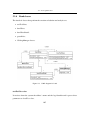
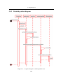
Il seguente schema illustra le connessioni esistenti tra gli elementi che compongono il
sistema ed il flusso di dati scambiato:
Figura 1.1.
Elementi del sistema
Come illustra la figura, il sistema è composto essenzialmente da tre parti:
• base di dati: contiene i dati relativi a tutti gli atleti e agli allenatori; la grande
maggioranza dei dati è rappresentata delle informazioni generate automaticamente
dai pulsometri. Solamente una minima parte è inserita manualmente dell’utente;
VIII
ulteriori dati, in numero decisamente inferiore, provengono dalle elaborazioni del
programma sui dati originali.
• Software +Atleta: permette all’utente di avere una visione completa dei suoi dati
di allenamento o di gara; tali dati possono essere piani di allenamento, viste grafiche
dei parametri fisiologici oppure dati completi sulle corse. I dati sono analizzati dal
software per ricavare parametri più complessi e specifici. Il software gestisce la
connessione sia con il database che con i dispositivi esterni.
• Pulsometro: origina la maggior parte dei dati presenti nel database; essi sono i dati
immagazzinati durante ogni gara od allenamento.
1.2.1
La base di dati
La base di dati è composta da tabelle che contengono tutte le informazioni del sistema.
Il database è stato progettato per contenere una grande quantità di dati. Dovrà immagazzinare, infatti, i dati di numerose squadre di atletica, ciascuna delle quali composta
mediamente da 20 corridori. Le informazioni sono rappresentate da dati personali, parametri biologici, caratteristiche di ciascun atleta e dati relativi ad ogni gara o sessione
di allenamento effettuati. Solamente i dati topografici dei percorsi non sono presenti nel
database. Questo è dovuto al fatto che essi sono in numero eccessivamente elevato e di
conseguenza non risulta conveniente salvarli all’interno del sistema locale, visto il loro
utilizzo poco frequente; è stato deciso di reperire tali informazioni da file esterni nel caso
in cui debbano essere analizzate dal programma. Infine, è opportuno precisare che si utilizza una base di dati MySQL [4], in grado di fornire tutte le funzionalità richieste senza
alcun costo di licenza. Si accede ai dati contenuti nel database mediante l’utilizzo delle
librerie MySQL++ [13].
IX
1.2.2
Il software +Atleta
Il software +Atleta è stato sviluppato usando il linguaggio di programmazione ad oggetti
Visual C++ [1] e l’ambiente di sviluppo Microsoft Visual Studio 2005 [6]. L’applicazione implementata utilizza inoltre i componenti ActiveX e la libreria MFC (Microsoft
Foundation Class library).
Per comprendere il funzionamento del programma esistente, è necessario esaminarne
le caratteristiche:
• Organizzazione delle informazioni: i dati sono suddivisi in tre grandi categorie,
in base alla funzione che ricoprono all’interno del programma. Esse sono:
– log: sono i dati provenienti dal pulsometro propriamente detti. Ciascuno di essi fa riferimento ad un’unica sessione di allenamento. Tutti i dettagli originali
sono visualizzati, ciascuno con la propria unità di misura.
– Piani di allenamento: corrispondono agli allenamenti tipo che possono essere
organizzati ed elaborati.
– Programmi di allenamento: sono raggruppamenti di più piani di allenamento,
secondo un denominatore comune.
• Funzioni svolte: al momento attuale sono disponibili le seguenti funzioni, raggruppate per grandi aree tematiche:
– sicurezza: la riservatezza dei dati è garantita dalla possibilità di effettuare il
login con la propria password. Gli account possono essere creati ed esistono
due tipi di utente: l’allenatore e l’atleta. Mentre il primo ha a disposizione i
dati personali ed i log relativi a tutti gli atleti della sua squadra, l’utente atleta
può solamente visualizzare i propri. Le informazioni utenti possono essere
modificate o cancellate in qualsiasi momento.
– Calendario: scegliendo il giorno del calendario è possibile associare ad una
particolare data più piani di allenamento e/o più programmi di allenamento.
X
– Log: può essere importato o esportato all’esterno, attraverso l’utilizzo di un
file in formato XML. Il log può essere modificato dall’utente o dall’allenatore.
È possibile vedere quale piano è associato ad un log, raggruppare più log sotto
una matrice comune ed effettuare la divisione di un log in più parti in relazione
alla sua durata.
– Confronto di log: è possibile effettuare il confronto di due log ed il programma
ne mostra i rispettivi valori, il valore massimo, minimo e medio tra i due.
– Grafici: il software prevede la visualizzazione grafica di alcuni parametri di
un log in relazione al tempo ed allo spazio: frequenza cardiaca, altitudine,
velocità e consumo energetico.
1.2.3
Il pulsometro
Il pulsometro è lo strumento usato per introdurre i parametri biologici degli atleti all’interno del sistema. Ciascun atleta che coopera allo sviluppo di questo progetto, deve
necessariamente allenarsi indossando un pulsometro. Al termine di ciascuna sessione di
allenamento, deve trasferire tutti i dati sul proprio PC, in quanto il pulsometro generalmente possiede una memoria piuttosto limitata. Durante la fase iniziale della tesi, sono
state effettuati approfonditi studi per stabilire quali informazioni immagazzinare nella base di dati e quali invece scartare. In particolare, sondando il mercato, sono stati scelti tre
produttori che offrono prodotti di ottima fattura: GARMIN [1], POLAR [2] e SUUNTO
[3].
Le pagine web dei produttori offrono informazioni dettagliate riguardo le caratteristiche dei propri prodotti, per cui è stato possibile confrontarle tra loro. In questa fase
dello sviluppo del progetto, sono stati presi in considerazione solamente i modelli che
rientrassero nella categoria “corsa”.
XI
1.3
Software statistico
Una parte importante del lavoro di tesi ha riguardato la creazione della struttura atta ad
eseguire l’analisi statistica dei dati. La base di dati MySQL, infatti, non fornisce strumenti
sufficienti per questo scopo. Dalle ricerche effettuate in questo senso, è emerso che la
soluzione migliore è quella di non implementare alcuna funzione statistica manualmente,
ma utilizzare software apposito già esistente. Questa soluzione è la conseguenza delle
seguenti considerazioni: implementare ciascuna singola funzione statistica richiede un
grande lavoro in termini di tempo per scriverne il codice e per comprendere a fondo la
teoria matematica su cui si basa. Inoltre, si ha un’altissima probabilità di commettere
errori nell’algoritmo di calcolo. Utilizzando invece un software apposito sono garantiti
l’affidabilità, il livello di precisione richiesti, la velocità di esecuzione e la semplicità.
Sul mercato si trovano numerosi software statistici dalle caratteristiche simili, come
SPSS, MINITAB o R. Per svolgere questa parte del lavoro di tesi, è stato scelto di utilizzare
R, poichè esso offre alcuni importanti vantaggi: non ha costi di licenza, è un software
open-source ed è in continuo sviluppo da parte della nutrita community di utenti. Proprio
per quest’ultimo motivo, R è un prodotto sempre più utilizzato da Professori e ricercatori
universitari. R offre inoltre gli strumenti per essere utilizzato in remoto da qualsiasi altro
software e la sua esauriente documentazione al riguardo ne hanno fatto lo strumento ideale
per gli scopi del progetto. In questa sezione verrà descritta l’infrastruttura creata per
integrare le funzionalità di R all’interno del software +Atleta. In particolare, si sottolinea
che l’obiettivo di questa attività non è stato quello di eseguire complesse analisi statistiche,
bensı̀ quello di creare l’infrastruttura affinchè i futuri ricercatori che collaboreranno al
progetto possano utilizzarla per sfruttare al meglio le potenzialità offerte da R. La sola
analisi statistica implementata è stata la regressione lineare dei parametri biologici degli
atleti presenti nel database.
XII
1.3.1
Collegamento ad R
Uno degli scopi del progetto +Atleta è quello di creare un modello di simulazione, per
poter calcolare in anticipo le prestazioni di un atleta. Numerosi solo gli input che devono
essere inseriti nel simulatore per svolgere la sua funzione; alcuni di essi sono i risultati relativi alle regressioni lineari effettuate usando R [8]. La regressione lineare è uno
strumento statistico che consente, date due variabili, di predirne una conoscendo il valore
dell’altra.
Le caratteristiche di R sono state dettagliatamente analizzate per poter ottenerne l’integrazione all’interno di +Atleta. Lo strumento utilizzato è denominato R SERVER; esso
è stato creato da alcuni sviluppatori di R e consente di connettere il software statistico con
qualsiasi altra applicazione scritta con i più comuni linguaggi di programmazione.
R SERVER è definito come un “DCOM server che contiene un’interfaccia COM a R”.
Per comprenderne la definizione è necessario conoscere la nomenclatura di tali acronimi:
COM (Component Object Model) è una piattaforma software introdotta da Microsoft [5] nel 1993. Questa tecnologia, nata per permettere la comunicazione tra processi e
la creazione dinamica di oggetti, si adatta ad ogni linguaggio di programmazione che la
supporti. I componenti/oggetto COM sono implementati in un linguaggio “neutrale”, non
conosciuto da chi ne fa uso, e possono essere visti come una scatola chiusa di cui non si
conoscono i meccanismi interni. Tali oggetti possono essere inseriti in qualsiasi ambiente
ed utilizzati mediante l’interfaccia di cui sono provvisti.
DCOM (Distributed Component Object Model) è un’altra tecnologia sviluppata da
Microsoft, per consentire la comunicazione tra componenti software distribuiti su una rete
di computer. DCOM estende dunque il concetto COM, aggiungendovi la gestione della
comunicazione distribuita tra oggetti.
XIII
Come descritto, gli oggetti COM/DCOM definiscono uno standard per l’interoperabilità ed assumono una funzione molto simile a quella di una libreria. Questa tecnica
di programmazione, simile al paradigma “ad oggetti”, è più correttamente definita “a
componenti”. Un componente è fondamentalmente una unità base che può incapsulare al
suo interno funzioni (metodi), dati (proprietà) e stati.
In riferimento a quanto detto, è importante conoscere la corretta nomenclatura:
• un componente è detto “COM/DCOM server”;
• l’utilizzatore di un componente è detto “COM/DCOM client”.
Il package R SERVER contiene un DCOM server utilizzato per connettere un’applicazione client con R. Come è stato accennato in precedenza, il package R SERVER fornisce
un’interfaccia COM a R, esattamente nello stesso modo in cui oggetti COM e controlli
ActiveX le forniscono alle applicazioni che li supportano. R (D)COM server possiede i
meccanismi per connettersi con:
• applicazioni standard (ad esempio Microsoft Excel);
• applicazioni scritte in qualsiasi linguaggio di programmazione, che svolgono la
funzione di COM/DCOM client; esse usano il motore computazionale di R e ne
ricavano gli output grafici e testuali.
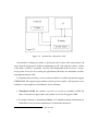
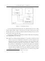
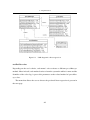
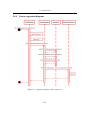
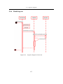
La figura nella pagina seguente mostra le relazioni esistenti tra gli elementi appena
descritti [11].
XIV
Figura 1.2.
Struttura del collegamento ad R
Osservando lo schema precedente si può notare che il cuore della connessione è R
server, il quale rappresenta l’anello di congiunzione tra R1 ed il software +Atleta. +Atleta
è l’R client, al quale è consentito l’accesso alle funzionalità di R. R server è in grado di gestire il caso in cui vi siano più applicazioni (R client) che intendano accedere
contemporaneamente ad R.
La comunicazione tra client e server avviene mediante lo scambio di particolari oggetti
COM/DCOM. Tali oggetti rappresentano il mezzo grazie al quale i dati possono essere
scambiati e sono composti essenzialmente da due elementi:
• l’interfaccia COM, che contiene i metodi e le proprietà (variabili) visibili dal
client. L’interfaccia rappresenta l’unico punto di accesso all’oggetto COM.
• Il secondo elemento è denominato Coclass ed è l’implementazione dell’interfaccia
COM. Più Coclass possono implementare la medesima interfaccia.
1
R deve necessariamente essere installato sulla macchina.
XV
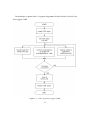
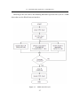
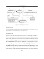
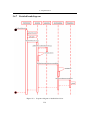
In riferimento a quanto detto, il seguente diagramma di flusso illustra il ciclo di vita
di un oggetto COM:
Figura 1.3. Ciclo di vita di un oggetto COM
XVI
1.3.2
Regressione lineare usando R
Utilizzando il software statistico R, la regressione lineare tra due variabili può essere
effettuata in pochi passaggi [12]:
1. dichiarazione delle variabili: ciascuna variabile deve essere inserita in forma di
vettore;
2. comando per la regressione lineare: usando il comando lm, viene eseguita la regressione lineare tra due variabili;
3. visualizzazione dei dati: con il comando plot si ottiene la rappresentazione Cartesiana (scatterplot) delle variabili;
4. retta di regressione: il comando abline visualizza la retta di regressione calcolata;
5. visualizzazione dei risultati: utilizzando summary si possono vedere tutte le informazioni relative alla regressione lineare calcolata.
L’esempio seguente chiarisce ulteriormente quanto descritto:
1.3.3
Motivazioni biomediche della regressione lineare
Il software +Atleta esegue, per il momento, solamente regressioni lineari tra due variabili. Tali variabili sono state selezionate in base alla rilevanza delle informazioni che
forniscono sotto il profilo medico/sportivo [14]:
XVII
1. FREQUENZA CARDIACA - VELOCITÀ: Il fattore risultante di questa regressione lineare è certamente quello che riveste maggiore importanza. Conoscendo la
relazione che intercorre tra frequenza cardiaca e velocità si può stimare il livello
di allenamento atletico di una persona. Osservando questo parametro si nota se
sia necessario o meno variare il carico di lavoro in allenamento per migliorare il
rendimento dell’atleta. Per esempio, un’alta velocità di corsa conseguita con una
frequenza cardiaca relativamente bassa è indice di un ottimo livello di allenamento.
2. FREQUENZA CARDIACA - ALTITUDINE: il fattore che può essere osservato è
l’adattabilità del fisico all’altitudine. Ad altitudini elevate (circa 2000 m) svolgere esercizio fisico è più faticoso che ad altitudini inferiori; questo fatto è la conseguenza della minor concentrazione di ossigeno nell’aria, che porta all’innalzamento
della frequenza cardiaca e di quella respiratoria.
3. FREQUENZA CARDIACA - DISTANZA: il suo sviluppo indica se l’atleta è allenato sulla lunga distanza. Questo è un fattore di secondaria importanza rispetto a i
primi due, ma rappresenta in ogni caso un aspetto da considerare.
4. VELOCITÀ - ALTITUDINE: questo parametro è molto simile a quello descritto
nel punto 2. Mantenere un’alta velocità ad alta quota è decisamente più difficile
che non ad altitudini inferiori.
5. VELOCITÀ - ENERGIA: assume significato solamente se considerato in associazione con valori della frequenza cardiaca, distanza e pendenza. Tale fattore è molto
particolare, in quanto non indica un parametro fisico, bensı̀ uno psicologico. Esso
segnala infatti se un atleta si trova a suo agio o meno nella corsa ad una particolare
velocità. Alcuni atleti prediligono la corsa a bassa intensità, ma per lunghe distanze;
alcuni corridori non si sentono a proprio agio percorrendo tratti in discesa, altri
ancora consumano eccessive energie nei tracciati in salita.
6. VELOCITÀ - DISTANZA: questo valore va associato all’analisi tra frequenza cardiaca e distanza [15]. Esso indica il comportamento del fisico sulla lunga distanza,
XVIII
è utile per capire se un atleta è in grado o meno gestire e razionare le proprie risorse
lungo tutto il percorso di gara, in modo tale da mantenere una prestazione costante.
1.4
Algoritmo di analisi dello sforzo fisico
Per poter essere ritenuta efficace, una sessione di allenamento deve provocare un cambiamento all’interno dell’equilibrio fisico di un atleta. Questo particolare fenomeno è
detto omeostasi. Ogni esercizio fisico è di per sè stancante, ma dopo l’allenamento,
durante la fase denominata di recupero, il normale stato fisico viene ristabilito. Il fisico si adatta allo sforzo richiesto dall’esercizio svolto in modo tale da poterlo affrontare
nuovamente, ma con prestazioni migliori; questo fenomeno è conosciuto con il nome di
supercompensazione.
Per conoscere il livello di supercompensazione e la giusta frequenza degli allenamenti,
è determinante stabilire il livello di sforzo di una sessione di allenamento. Il metodo che
è stato utilizzato nella tesi per calcolare lo sforzo è lo stesso suggerito nel manuale di
utilizzo del software “POLAR Precision Performance” [2].
Un altro importante fattore da considerare è il tempo di riposo necessario. Esso dipende sia dall’intensità dell’allenamento (frequenza cardiaca) che dalla sua durata. Risulta
necessario organizzare la frequenza degli allenamenti, lasciando passare il tempo opportuno tra due allenamenti successivi: non devono essere troppo ravvicinati per evitare il
sovrallenamento e non devono essere troppo distanti da non risultare efficaci.
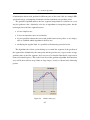
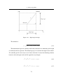
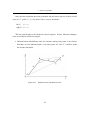
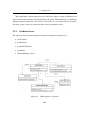
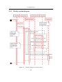
Figura 1.4. Rappresentazione degli effetti di un allenamento sulle prestazioni. Sull’asse
delle ascisse è presente la durata e sull’asse delle ordinate l’intensità di un allenamento
XIX
Come si evince dallo schema precedente gli effetti immediati di un esercizio sono
la diminuzione delle prestazioni. Dopo l’esercizio si entra nella fase di recupero, durante la quale la curva delle prestazioni cresce lentamente fino a raggiungere il livello
iniziale. La fase successiva è quella della supercompensazione, nella quale il livello delle prestazioni aumenta fino a superare quello iniziale. Per incrementare visibilmente le
prestazioni di un atleta, l’allenamento successivo deve sempre avvenire all’interno fase di
supercompensazione.
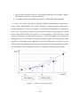
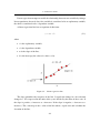
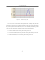
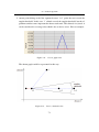
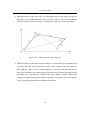
Il calcolo dello sforzo fisico è stato ideato in modo tale da ricavare un parametro numerico avendo come dati iniziali lo sport praticato, la durata e l’intensità dell’allenamento.
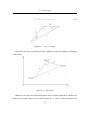
Figura 1.5.
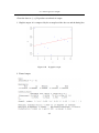
Relazione tra sforzo fisico e tempo di recupero
La figura precedente mostra, per esempio, che con un valore di sforzo pari a 300,
la relativa fase di recupero deve esse circa un giorno. Terminata questa fase l’atleta è
pronto per compiere un nuovo allenamento, poichè il suo fisico si trova nella fase di
supercompensazione.
Come anticipato in precedenza, il calcolo numerico dello sforzo fisico è il risultato
della combinazione di tre elementi dell’allenamento:
1. durata (tempo, espresso in minuti);
2. intensità (frequenza cardiaca, espressa in battiti al minuto);
3. coefficiente sportivo (coefficiente che dipende dallo sport praticato).
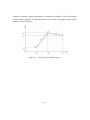
XX
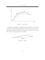
Per ciascun intervallo di frequenza cardiaca, è dato un coefficiente di sforzo per il
quale è moltiplicato il tempo trascorso in tale intervallo. Il tutto è poi moltiplicato per il
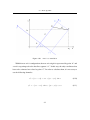
coefficiente relativo allo sport praticato. La formula è la seguente:
Sf orzo =
n
X
[(CSf dell0 intervallo di f requenza) · (tempo trascorso)] · (CSp ) (1.1)
i=0
dove:
• CSf è il Coefficiente di Sforzo;
• CSp è il Coefficiente Sportivo;
• i è l’indice degli intervalli di frequenza cardiaca;
• n è il numero degli intervalli di frequenza cardiaca.
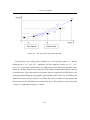
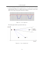
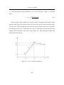
Il coefficiente di sforzo relativo a ciascun intervallo di frequenza è stato ricavato in
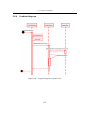
relazione al seguente grafico:
Figura 1.6.
Sforzo relativo in funzione della frequenza cardiaca
Il valore dello sforzo fisico è tipicamente compreso tra 50 e 400, mentre il valore del
coefficiente sportivo oscilla tra 0.8 e 1.3.
Per quanto concerne l’implementazione, il software utilizza l’algoritmo per visualizzare graficamente il valore dello sforzo fisico di un atleta, consentendo all’utente di
XXI
scegliere la finestra temporale mensile o settimanale. Per ciascun allenamento sono mostrati inoltre importanti parametri associati, quali i valori minimo, massimo e medio sia
della frequenza cardiaca che della velocità. Il coefficiente sportivo e quello di sforzo
relativo a ciascun intervallo di frequenza possono essere modificati a piacere dall’utente;
in tal caso il software ricalcolerà nuovamente tutti i parametri.
1.5
Algoritmo di analisi della pendenza del tracciato
Un’altra analisi molto interessante riguarda le prestazioni degli atleti in relazione allo
sviluppo altimetrico della corsa. Gli atleti possono avere un comportamento molto differente in termini di velocità o consumo energetico a seconda della pendenza del tracciato.
Per esempio, alcuni corridori potrebbero presentare caratteristiche di grande resistenza in
salita, ma possedere una tecnica di corsa in discesa non efficace. Analizzando il profilo del
percorso in relazione ai parametri biologici degli atleti è possibile evidenziare limiti fisici
o atletici, in maniera tale da poter adeguatamente pianificare allenamenti che suppliscano
a tali carenze.
L’algoritmo ideato, partendo dai valori puntuali della distanza e della altitudine, rappresentati rispettivamente sull’asse delle ascisse e su quello delle ordinate, crea un profilo
altimetrico modificato. L’algoritmo associa tra loro i segmenti che presentano una pendenza simile, presentando un profilo altimetrico meno frastagliato rispetto a quello ottenuto con i dati originari. Tale profilo inoltre può essere studiato con molta più semplicità;
esso mette in relazione ciascun tratto del percorso con pendenza costante con parametri
quali la frequenza cardiaca, la velocità ed il consumo energetico.
L’algoritmo utilizza l’interpolazione mediante segmenti per calcolare il valore della
pendenza. Esistono molteplici metodi per l’interpolazione di punti, ma si è scelto questo
in relazione alle seguenti considerazioni:
• è il metodo più semplice;
• non introduce rumore nel calcolo;
XXII
• dato che non è possibile conosce l’esatto profilo altimetrico tra due punti, è impossibile stabilire quale sia l’algoritmo migliore;
• è possibile ottenere molti livelli di precisione, modificando alcuni parametri.
L’idea su cui si basa l’algoritmo è quella di scandire completamente il vettore contenente il valore dell’altitudine. Per ciascun elemento si esegue la seguente elaborazione:
un punto appartiene ad un certo segmento, se la pendenza del segmento che congiunge il
punto stesso ed il punto precedente non eccede una determinata soglia angolare, stabilita
in base alla pendenza media del segmento a cui fa riferimento. Nella realtà però, alcuni
percorsi presentano dei profili molto particolari: si pensi ad esempio ad un tracciato di
montagna dove ci sono numerosi saliscendi. Per questa ragione sono stati presi in esame
più punti (e di conseguenza più segmenti) nel calcolo dell’algoritmo, in modo tale da considerare anche la tendenza futura del percorso in questione. In questo modo è possibile
non considerare lievi oscillazioni del terreno o valori non corretti dei dati in origine.
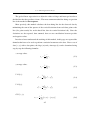
Figura 1.7.
Punti coinvolti nell’algoritmo
XXIII
L’algoritmo di calcolo decide se il punto esaminato (“i”) appartiene ad un segmento dopo aver effettuato tre test. Come mostra la figura precedente, il sistema calcola le
pendenze dei segmenti “S1”, “S+1”, ed “S+2” che congiungono rispettivamente i punti
“i”, “i+1” e “i+2” con il punto precedente a quello considerato (“i-1”). Se almeno una
delle tre pendenze cosı̀ calcolate non eccede la pendenza media del segmento di riferimento, il punto è considerato parte del segmento generale e l’algoritmo procede verso i
punti successivi del tracciato. La figura seguente mostra un esempio del profilo che si può
ottenere:
Figura 1.8. Profilo mostrato da +Atleta. In blu il tracciato originale, in rosso
quello elaborato dell’algoritmo
La classe implementata gradientView visualizza sia il profilo altimetrico originale del
tracciato che quello ottenuto dall’elaborazione dell’algoritmo. Numerosi parametri statistici associati sono mostrati in forma riassuntiva, suddivisi per range di pendenza: pendenza massima e minima, numero di segmenti appartenenti al range e loro percentuale
sul totale, frequenza cardiaca massima e media e per concludere velocità massima e media. Il limite angolare utilizzato può essere modificato dall’utente; in tal caso il software
provvede in pochi istanti a rieseguire l’algoritmo ed aggiornare le statistiche. L’interfaccia contiene infine un apposito bottone che consente di vedere le statistiche complete di
ciascun segmento individuato dall’algoritmo.
XXIV
1.6
Algoritmo di analisi delle curve del tracciato
Partendo dalle semplici coordinate topografiche, questa analisi ha l’obbietivo di stabilire
il numero di curve di un percorso e la loro direzione. L’importanza di conoscere queste
informazioni risiede nel fatto che ciascun atleta ha una la propria tecnica di corsa che
dipende enormemente dalla propria gamba preferita. La simmetria del corpo umano non
è perfetta, per cui la potenza degli arti inferiori di ciascun individuo non è distribuita
equamente. Ciò si traduce in una differenza in termini di velocità e consumo energetico
a seconda che l’atleta percorra una curva a destra piuttosto che una a sinistra. Per questo
motivo percorrere un tracciato in una direzione o in quella opposta può comportare una
differenza di prestazione.
L’algoritmo implementato prende in esame il tracciato di gara o di allenamento, rappresentandolo ed esaminandolo come una sequenza di segmenti. I dati a disposizione
sono le coordinate topografiche rilevate utilizzando un apparecchio GPS (Global Position
System) e sono rappresentati mediante un grafico Cartesiano. Le coordinate Cartesiane
vengono trasformate in coordinate Polari per una più semplice analisi: in questo modo
non si hanno a disposizione punti, ma segmenti. L’elaborazione successiva coinvolge
una coppia di segmenti adiacenti alla volta: a seconda dell’ampiezza dell’angolo tra essi
compreso, si presenta uno dei seguenti casi:
• se il valore angolare è molto elevato e supera la soglia prestabilita (angolo limite),
non c’è alcuna curva;
• se l’angolo ha un’ampiezza che non supera l’angolo limite si presentano due alternative:
– si è in presenza di una curva se la curva precedente è più distante di una certa
soglia (distanza limite) oppure se la curva precedente è nell’altra direzione;
– non c’è una nuova curva, poichè quella in esame fa parte di una curva più
grande, delimitata da più di due segmenti consecutivi.
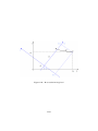
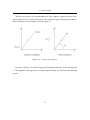
L’algoritmo compie una roto-traslazione degli assi cartesiani per ogni coppia di segmenti adiacenti, in modo tale da sovrapporre l’asse delle ascisse con il primo dei due
XXV
segmenti considerati. Questa operazione è essenziale per stabilire, in base alla posizione del secondo segmento, la direzione della curva in esame. Il seguente schema aiuta a
chiarire il concetto esposto:
Figura 1.9.
Configurazione standard degli assi
XXVI
Figura 1.10.
Roto-traslazione degli assi
XXVII
Riassumendo quanto detto finora, l’algoritmo riconosce in quale scenario si trova la
curva analizzata e ne provvede ad immagazzinare i parametri associati, quali la frequenza
cardiaca, la velocità, la pendenza ed il consumo energetico. Nel caso in cui una curva
sia composta da più di due segmenti consecutivi, i predetti parametri sono calcolati come
valore medio tra tutti quelli coinvolti.
Per quanto concerne l’implementazione, la classe bendView consente di visualizzare
la planimetria del tracciato e fornisce numerose statistiche associate, quali l’ampiezza
massima, minima e media dell’angolo della curva, la percentuale di curve a destra ed
a sinistra sul numero totale di curve, la frequenza cardiaca media, la velocità media e
la pendenza media. Esistono poi due tipi di statistiche riassuntive: la prima suddivide
le informazioni citate in intervalli di ampiezza di angolo della curva, mentre la seconda
raggruppa i valori in base a range di pendenza. Inoltre, l’interfaccia consente all’utente
di modificare i due importanti parametri coinvolti nell’algoritmo: l’angolo limite e la
distanza limite. Se tali parametri vengono modificati, il software riesegue l’algoritmo ed
aggiorna i valori delle statistiche. L’utente ha la possibilità di consultare i dati esaustivi
relativi a ciascuna curva cliccando sull’apposito bottone.
1.7
Conclusioni
Al termine del lavoro effettuato si possono trarre le conclusioni su ciò che è stato conseguito. L’attività di tesi ha portato alla definizione di nuove ed importanti funzionalità del
software +Atleta. In particolare è stata creata la struttura atta a compiere la regressione
lineare dei dati presenti nel database del sistema. Attraverso un’opportuna interfaccia,
è possibile scegliere su quali dati effettuare la regressione lineare ed automaticamente il
sistema provvede a connettersi ad R, inviare le informazioni necessarie e ricevere il risultato delle elaborazioni in pochi istanti. Queste ultime sono mostrate all’utente sotto forma
grafica e corredate dai più importanti dati statistici associati. La regressione lineare non si
effettua su tutti i dati biologici che si hanno a disposizione, ma solamente su quelli che sono stati selezionati in base alla rilevanza che assumono dal punto di vista medico-sportivo.
XXVIII
L’obiettivo di questo lavoro non è stato quello di effettuare profonde ed elaborate analisi
statistiche dei dati, bensı̀ quello di impostare una infrastruttura semplice ed efficace affinché tali analisi possano aver luogo. È stata in questo modo ideata la base sulla quale
si fonda il lavoro di altri ricercatori che collaboreranno al progetto, i quali disporranno di
uno strumento funzionante e potranno sfruttare la dettagliata documentazione al riguardo
per utilizzare al meglio le grandi potenzialità che offre il software statistico R.
Inoltre, gran parte del lavoro di tesi è stato quello di ideare e realizzare tre algoritmi di
analisi di dati relativamente allo sforzo fisico dell’atleta, al profilo altimetrico del percorso di gara ed alla planimetria della corsa. Tali analisi si occupano di particolari e delicati
aspetti della preparazione atletica ed hanno lo scopo di visualizzarne approfondite e dettagliate statistiche; rivestono inoltre un ulteriore funzione: quella di calcolare determinati
parametri che potranno essere utilizzati come input per il DSS che verrà implementato
nei prossimi anni, utile per prevedere le prestazioni di un atleta in una competizione non
ancora avvenuta. Infine, per facilitarne la diffusione e l’utilizzo, seppur per il momento
solamente in ambito accademico, è stato realizzato un comodo installatore per i sistemi operativi Microsoft. Esso installa in pochi passaggi il software +Atleta, il database
MySQL e tutti i componenti aggiuntivi necessari per il coretto funzionamento.
Per quanto riguarda invece la realizzazione dei componenti software, si è cercato di
favorire l’aspetto architetturale della progettazione, cercando di suddividere il più possibile ciascun ambito e di utilizzare un approccio modulare. Grazie ad esso è stato possibile
fornire un certo grado di estensibilità, mediante la quale sarà possibile aggiungere nuove
funzionalità al progetto, senza doverne necessariamente modificare l’intera architettura.
Uno dei principi che ha guidato il lavoro di tesi è stato cercare di rendere le diverse componenti il più possibile compatibili con il resto del sistema, anche sotto il profilo grafico,
in maniera tale da rispettare e seguire le linee guida tracciate da chi vi ha lavorato precedentemente. Un ulteriore scelta progettuale è stata quella di continuare ad usare standard
e raccomandazioni ampiamente accettate a livello internazionale per la realizzazione di
ogni componente: ne sono esempi la creazione del collegamento con il software statistico
XXIX
mediante R-server, strumento in continuo aggiornamento e sviluppo che garantisce grande longevità al progetto oppure l’utilizzo della tecnologia ActiveX per la visualizzazione
di tutti i grafici. Da sottolineare infine, che l’attività di creazione delle interfacce utente
è stata eseguita ponendo particolare attenzione alla semplicità, intuitività ed immediatezza nel loro utilizzo; ciascuna interfaccia è stata concepita in modo tale da possedere due
livelli di precisione: un livello principale nel quale sono contenute le informazioni che
rivestono un ruolo fondamentale ed un riassunto dei dati suddivisi per categoria, ed un livello secondario più approfondito e completo, riservato agli utenti con necessità di vedere
informazioni dettagliate su un determinato tema.
Come già evidenziato più volte all’interno della tesi, il lavoro svolto all’interno del
progetto +Atleta ha riguardato la terminazione dell’intera infrastruttura del sistema. Tuttora il progetto si trova in fase di pieno sviluppo e molti sono i collaboratori che ne prendono parte, ognuno di essi occupandosi di un aspetto specifico. Le tematiche in questione
sono numerose e affrontano sia lo sviluppo di nuove funzionalità che il miglioramento
di quelle esistenti; ad esempio vi è lo scambio di dati tra i pulsometri professionali ed il
sistema che non è ancora automatico e semplice come dovrebbe essere quello di un software che vuole incontrare un numero elevato di utenza. Inoltre, il lavoro da me svolto si
occupa unicamente del funzionamento su una singola macchina. Alcuni ricercatori stanno realizzando un sistema distribuito, grazie al quale si potrà accedere alle funzionalità
del software anche attraverso il web; in questo caso l’architettura tradizionale del sistema
verrà rivoluzionata per assumere la conformazione tipica del modello client-server. In altre parole, quello che si vuole ottenere è una scissione netta tra il software, che rappresenta
il motore dell’applicazione, ed il database che ne contiene le informazioni.
Il progetto +Atleta prevede due tipi di prospettive future: la prima riguarda il breve
periodo mentre la seconda è a lungo termine. Nel prossimo futuro, nell’arco di duo o tre
anni, è prevista l’ultimazione del progetto generale con la messa a punto sia del simulatore
che del DSS. Entro questo periodo ci si propone inoltre di estendere le funzionalità del
software, riservate per il momento solo alla corsa, a molte altre discipline dell’atletica.
A lungo periodo invece, una volta che il sistema risulti perfettamente funzionante sugli
XXX
atleti, ne è prevista l’applicazione in campo medico. L’idea nasce dal fatto che, una volta
conosciuti i dati relativi al comportamento di un fisico sano, eventuali parametri che si
discostino eccessivamente da essi potrebbero essere sintomo di disfunzioni o patologie;
in questo caso +Atleta diverrebbe un utilissimo strumento di prevenzione.
XXXI
Summary
The goal of this thesis is to describe my work of cooperation done at the UPC (Universitat Politècnica de Catalunya) and to intensify the knowledge about the related theoretical
aspects. As my work is concerned, it can be described as a collaboration in the +Atleta
project. It begun in 2005 and nowadays it is still in phase of development. The goal
of this project is the creation of a DSS (Decision Support System) for sport activities,
that is a software for professional use whose aim is to help an athlete to improve his/her
performances. By starting from deep analysis of body parameters, the software will be
able to simulate the future performances of the athlete. This thesis work is focused on
the improvement of the existing project, adding on new functionalities and capabilities.
In this phase of project development, the attention is focused on creating the main infrastructure that could allow performance simulation in the future. Numerous data have to be
taken into consideration, some of them are: body parameters, training or race courses and
whether conditions. In particular, data which have been studied and implemented are data
analysis about body exertion, altimetric track profile and topographic track profile. This
analysis has involved the creation of many statistical views, grouped into thematic areas,
and statistical analysis of some important factors using linear regression. The work had
started from the knowledge of the existing project and, through the technical analysis of
the infrastructure creation, it finished with the implementation of new software functionalities. In the present document, objectives, planning methods and development phases
which have been developed during the thesis period are described in detail. Finally, a final
evaluation about the work done, as well as the conclusions and the considerations about
the future of the project, are present in this thesis.
XXXIII
Acknowledgements
This research activity would not have been possible without the contributions of the Prof.
Pau Fonseca i Casas and the Prof. Elena Baralis. I am grateful for his and her time,
suggestions and detailed comments. On my personal side, I would like to acknowledge
my family, who has always supported me during these years at the University and has
believed in me.
XXXV
Contents
Sommario
III
1.1
Introduzione . . . . . . . . . . . . . . . . . . . . . . . . . . . . . . . . .
IV
1.2
Descrizione del sistema esistente . . . . . . . . . . . . . . . . . . . . . .
VIII
1.3
1.2.1
La base di dati . . . . . . . . . . . . . . . . . . . . . . . . . . .
IX
1.2.2
Il software +Atleta . . . . . . . . . . . . . . . . . . . . . . . . .
X
1.2.3
Il pulsometro . . . . . . . . . . . . . . . . . . . . . . . . . . . .
XI
Software statistico . . . . . . . . . . . . . . . . . . . . . . . . . . . . . .
XII
1.3.1
Collegamento ad R . . . . . . . . . . . . . . . . . . . . . . . . .
XIII
1.3.2
Regressione lineare usando R . . . . . . . . . . . . . . . . . . .
XVII
1.3.3
Motivazioni biomediche della regressione lineare . . . . . . . . .
XVII
1.4
Algoritmo di analisi dello sforzo fisico . . . . . . . . . . . . . . . . . . .
XIX
1.5
Algoritmo di analisi della pendenza del tracciato . . . . . . . . . . . . . .
XXII
1.6
Algoritmo di analisi delle curve del tracciato . . . . . . . . . . . . . . . .
XXV
1.7
Conclusioni . . . . . . . . . . . . . . . . . . . . . . . . . . . . . . . . .
XXVIII
Summary
XXXIII
Acknowledgements
XXXV
1
Introduction
1
2
Existing project
5
2.1
5
Project planning . . . . . . . . . . . . . . . . . . . . . . . . . . . . . . .
XXXVII
3
4
2.2
Current situation . . . . . . . . . . . . . . . . . . . . . . . . . . . . . .
9
2.3
Project guidelines . . . . . . . . . . . . . . . . . . . . . . . . . . . . . .
10
2.4
Project description . . . . . . . . . . . . . . . . . . . . . . . . . . . . .
11
2.4.1
Database . . . . . . . . . . . . . . . . . . . . . . . . . . . . . .
13
2.4.2
+Atleta software . . . . . . . . . . . . . . . . . . . . . . . . . .
18
2.4.3
External devices . . . . . . . . . . . . . . . . . . . . . . . . . .
20
Statistical software
29
3.1
R connectivity . . . . . . . . . . . . . . . . . . . . . . . . . . . . . . . .
30
3.2
Embedding R in applications on MS Windows . . . . . . . . . . . . . . .
32
3.2.1
Interface IStatConnector . . . . . . . . . . . . . . . . . . . . . .
35
3.2.2
Data transfer . . . . . . . . . . . . . . . . . . . . . . . . . . . .
38
3.2.3
Error handling . . . . . . . . . . . . . . . . . . . . . . . . . . .
40
3.3
R connection example . . . . . . . . . . . . . . . . . . . . . . . . . . . .
41
3.4
Linear regression’s theory . . . . . . . . . . . . . . . . . . . . . . . . . .
43
3.5
Linear regression using R . . . . . . . . . . . . . . . . . . . . . . . . . .
48
3.6
Biomedical motivations . . . . . . . . . . . . . . . . . . . . . . . . . . .
52
Analysis algorithms
55
4.1
Exertion algorithm . . . . . . . . . . . . . . . . . . . . . . . . . . . . .
55
4.1.1
Calculating the exertion count . . . . . . . . . . . . . . . . . . .
58
4.1.2
The algorithm . . . . . . . . . . . . . . . . . . . . . . . . . . . .
63
Gradient algorithm . . . . . . . . . . . . . . . . . . . . . . . . . . . . .
64
4.2.1
The algorithm . . . . . . . . . . . . . . . . . . . . . . . . . . . .
73
Bend algorithm . . . . . . . . . . . . . . . . . . . . . . . . . . . . . . .
76
4.3.1
85
4.2
4.3
5
The algorithm . . . . . . . . . . . . . . . . . . . . . . . . . . . .
Implementation
89
5.1
Use cases . . . . . . . . . . . . . . . . . . . . . . . . . . . . . . . . . .
89
5.1.1
91
Log management . . . . . . . . . . . . . . . . . . . . . . . . . .
XXXVIII
5.1.2
5.2
5.3
Athlete management . . . . . . . . . . . . . . . . . . . . . . . .
94
Conceptual model . . . . . . . . . . . . . . . . . . . . . . . . . . . . . .
95
5.2.1
Linear regression classes . . . . . . . . . . . . . . . . . . . . . .
95
5.2.2
Exertion classes . . . . . . . . . . . . . . . . . . . . . . . . . . . 100
5.2.3
Gradient classes . . . . . . . . . . . . . . . . . . . . . . . . . . 104
5.2.4
Bend classes . . . . . . . . . . . . . . . . . . . . . . . . . . . . 107
Model of behaviour . . . . . . . . . . . . . . . . . . . . . . . . . . . . . 110
5.3.1
5.4
5.5
6
Operations . . . . . . . . . . . . . . . . . . . . . . . . . . . . . 110
Sequence diagrams . . . . . . . . . . . . . . . . . . . . . . . . . . . . . 111
5.4.1
Linear regression diagram . . . . . . . . . . . . . . . . . . . . . 112
5.4.2
Monthly exertion diagram . . . . . . . . . . . . . . . . . . . . . 113
5.4.3
Weekly exertion diagram . . . . . . . . . . . . . . . . . . . . . . 114
5.4.4
Gradient diagram . . . . . . . . . . . . . . . . . . . . . . . . . . 115
5.4.5
Detailed gradient diagram . . . . . . . . . . . . . . . . . . . . . 116
5.4.6
Bend diagram . . . . . . . . . . . . . . . . . . . . . . . . . . . . 117
5.4.7
Detailed bend diagram . . . . . . . . . . . . . . . . . . . . . . . 118
Setup creation . . . . . . . . . . . . . . . . . . . . . . . . . . . . . . . . 119
Conclusions
123
A Database specifics
127
B Code examples
139
B.1 XML file . . . . . . . . . . . . . . . . . . . . . . . . . . . . . . . . . . 139
B.2 Database access . . . . . . . . . . . . . . . . . . . . . . . . . . . . . . . 145
B.3 R connection . . . . . . . . . . . . . . . . . . . . . . . . . . . . . . . . 146
C Work planning
151
D Glossary
157
Bibliography
159
XXXIX
Web Sites
161
XL
Chapter 1
Introduction
At the present time, the competitiveness at professional level in the sport world is so
high that any way or instrument that could help to improve athlete’s performances has
been pursuing. In the last few years, the use of technology has become more and more
frequent, since people understood that its use in sport disciplines gave an improvement of
precedent results. Nowadays, at professional level, a little margin of improvement could
even mean the achieving of a new world record or, more simply, a new victory.
Human nature is very competitive and every person has the tendency to improve and
surpass himself and his limits, day by day. In order to achieve this important objective, it is necessary to always work at full capacity. For this reason, all parameters that
could improve the performances must be controlled. It exists nowadays a large number of
worldwide companies, indeed, that invest for years in this kind of projects. These projects
could involve a broad spectrum of activities: some producers make professional instruments capable of store body parameters of athletes, others offer analysis services of these
data as decision support system about the physical state of a person, others make special
sportswear depending on the sporting discipline. Furthermore, numerous new specialized
sports centers have been created, generally from sports clubs of great importance. There,
high technology and specialized staff are used to achieve the improvement of athletes’
performances.
1
1 – Introduction
Into this complex scenario, the project called “+Atleta” was born at the UPC (Universitat Politècnica de Catalunya) in Barcelona. This project, managed by the Professor Pau
Fonseca i Casas, is put in the area of interest of the body data analysis. It was devised
after a long and deep research about similar products present in the market. By analyzing
all the characteristics of +Atleta strong and weak points, its limitations, many possibilities of future improvements have been highlighted. Leader companies in this market’s
sector have been taken as a model; in particular, three worldwide companies: POLAR,
GARMIN and SUUNTO. They produce professional training computers and furnish to
their customers their own software. It provides to visualize and manage data retrieved
during any race or training session. Biological data are not subjected to deep analysis, but
in the majority of cases they are displayed as graph or table view. This means that these
software do not provide more information than the ones that training computers provide
in real time during a training session. Data are just visualized in a more comprehensible
form. Moreover, the customer must utilize the furnished software, because each company
has its own format data. This last point represents a considerable disadvantage, because it
is not possible to analyze data from products of different brands. As consequence of these
considerations, what has been occurred to mind was the idea of creating a new product
who can compensate lacks of existing ones. It overcomes their limitations and represents
a new alternative, especially for professional use. +Atleta project is an instrument who
can offer new capabilities in biological data analysis. It was born in September 2005 and
it is still now in phase of development. This is a long-term project, its aim is to create
a DSS (Decision Support System), a very complex software capable of doing a constant
and detailed monitoring of the sporting performance of numerous athletes. Furthermore,
it is able to perform deep data analysis to reach the athletes’ increasing performances.
Through the analysis of a great quantity of data, the DSS is a real simulation system and
its aim is to predict in advance, with particular atmospheric and environmental conditions,
future athlete’s results on a certain sport discipline, on a given track route.
The product’s lacks present on the market are transformed into the strong point of
this project. By using their training devices, +Atleta software is planned to be a standard
2
instrument able to obtain data from any device, independently from its brand or model.
Retrieved data are translated and mapped on a XML format file (see paragraph 2.4.3) and
subsequently stored into a MySQL database. On the one hand, data are shown to the user
as graph or table view, in order to highlight the most significant ones. On the other hand,
they are subjected to more complex elaboration and processes which calculate numerous
biological parameters. These estimated parameters represent the DSS’ input variables and
they assume an important role into the athlete’s performance simulation.
The goal of the present thesis is to describe my cooperation work and my assumed
role into the +Atleta project development. A large number of complex work phases are
needed to complete +Atleta project. They are described in the paragraph 2.1 (Project
planning) and are planned in such a manner that can be developed by several people at
the same time. A preparatory phase of the work was focused on the study of the existing
project’s architecture, functioning and on the project development. The amount of work
that has to be done is very high and is so complex that students and researchers with others
university careers are involved into the project. My work’s contribution is located in the
phase of completion of the existing system’s infrastructure, which is described in detail in
chapter 2. Two main aspects have been taken into consideration: the first is the creation
of the statistical data analysis structure, by the implementation of a connection with the R
software; the previous step was the study of R’s capabilities, then the attention has been
paid on the implementation of the linear regression, a particular statistical analysis which
provides interesting information about the physical state of an athlete. Nevertheless, the
main aim of this work has been the detailed structure documentation, the description of
every connectivity’s mechanism between R and +Atleta. In this way, future researchers
(specialized into sports medicine) will utilize it to do more complex, efficient and useful
data analysis. Chapter 3 explains what previously has been said. The second aspect taken
into consideration is the creation of three analysis algorithms related to athlete’s exertion,
track’s gradient and bends of the training way respectively. Their goals are to show statistics and to count parameters which can be used as input for the simulator engine. Their
theoretical aspects and functioning are described in detail in chapter 4. Chapter 5 of the
3
1 – Introduction
thesis explains algorithms’ implementation on Visual Studio 2005 framework. Moreover,
a special user-friendly interface which permits to use in a simple way the new +Atleta’s
functionalities has been implemented. Moreover, all characteristics, features, planning
decisions, classes architecture, use case diagrams and sequence diagrams are present, too.
Finally, chapter 6 contains the conclusions about the work that has been done, it describes
the current project’s situation and explains its future development.
4
Chapter 2
Existing project
2.1
Project planning
+Atleta is certainly a very ambitious project, that requires a big work in terms of time and
human resources. For this reason it has been planned and organized in such a manner to
be developed by numerous students, everyone with a different assigned work, depending
on the type and the level of their previous university careers. Due to its complexity, the
project development is organized as a multi-year activity, and it is possible to identify
three basic phases. Each one is divided into several sub-activities:
• infrastructure creation: it consists in software planning, requirement decision,
setting up its characteristics and its functional working, planning which functions
have to be implemented and finally deciding which kind of data utilize. This represents the base for the following development phases. For this reason, this infrastructure creation is divided into the following activities:
– determination of software requirements and its functions;
– determination of data type to be researched;
– determination of data format;
– determination of database structure and how to manage it;
– software implementation;
5
2 – Existing project
– parser implementation, to import and normalize data from external devices
that will be stored into the database;
– data visualization in a useful and comprehensible shape;
– data management;
– creation of statistical data analysis structure;
– creation of web access structure.
• Data retrieval: it represents a collaboration between project developers and different existing athletics teams. This phase is necessary to retrieve great quantities of
valid data. Its start is estimated on January 2008 and its duration is exactly one year.
The starting point is not a parameter as restrictive as the duration. The duration is
the most important factor of this development part of +Atleta project, because the
aim is to obtain training data of all seasons. This is due to the fact that it’s important
and useful compare the athlete’s performance related to the same training session,
but done in different seasons to study if and how climatic conditions affect it. Data
retrieval is divided into sub-activities:
– detection of athletes teams which cooperate with the project in question;
– detection of retrieval data procedure;
– retrieval data phase;
– validation data procedure;
– possible database modification.
• Data analysis: this final phase consists in finding the existing relationship, considered in forms of mathematical and statistical functions, between the parameters
studied and retrieved in the previous phases. This work has the goal of extrapolating
information from founded relations, and helping trainers to understand how athletes
performances can be improved. It involves a deep initial statistics study joined with
an excellent body parameters knowledge. The whole project terminates with the
DSS (Decision Support System) creation. It is a very complex work because it involves the use of a simulation model, to predict the future athlete’s performances.
6
2.1 – Project planning
A temporary simulation model implementation will be performed, then the establishment of the used variable, hypothesis and development paradigms. Models will
be created and implemented. The final simulation model will be ready after a deep
test session. Tests are divided into three parts: validation is used to establish if the
used simulation models are the correct ones. Verification is used to check if was
performed the right model implementation. The final step is accreditation, i.e. the
certification of a person, a body or an institution as having the capacity to fulfill this
particular function. A further difficulty is to choose which information have to be
shown to the user and in which way.
Data analysis phase is composed by:
– determination of work hypothesis;
– deep statistics data study;
– body parameters study;
– determination of relationship between different parameters;
– initial simulation model construction:
∗ determination of Variables;
∗ determination of Hypothesis;
∗ determination of Paradigms.
– Models implementation;
– tests:
∗ validation;
∗ verification;
∗ accreditation.
At the moment, considering this work’s contribution, +Atleta project is at the end of
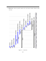
the first phase, infrastructure creation. In the next page it is possible to see the general
Gantt diagram of the project.
7
2 – Existing project
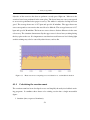
Figure 2.1.
General Gantt diagram
8
2.2 – Current situation
2.2
Current situation
The initial part of the present thesis is focused on the study and the analysis of the existing system. Making reference to the planning phases of the project described in the
previous paragraph, it is necessary to examine the present situation in order to proceed to
the accurate description of the thesis work.
Currently, +Atleta project is close to the end of the first planned phase (see project
planning paragraph). It means that this work and the one of others students involved in
the project development, is focused on the creation of the whole program infrastructure.
To carry out the infrastructure is a crucial step for software development. It is considered
one of most important milestones, because all the future developments have as base the
work done in this primary phase.
At the moment, the mentioned DSS takes only one sport into account: one is speaking about running, which behaves to the category of athletics. In particular, software is
planned to manage running in all its different forms:
• track events, running events conducted on a 400 m track:
– sprints: events up to and including 400 m. Common events are 60 m (indoors
only), 100m, 200m and 400m.
– Middle distance: events from 800m to 3000 m, 800m, 1500m, mile and
3000m. Belongs to this category the steeplechase - a race (usually 3000 m) in
which runners must negotiate barriers and water jumps.
– Long distance: runs over 5000 m. Common events are 5000 m and 10000 m.
Less common are 1, 6, 12, 24 hour races.
– Hurdling: 110 m high hurdles (100 m for women) and 400 m intermediate
hurdles (300 m in some high schools).
– Relays: 4 x 100m relay, 4 x 400 m relay, 4 x 200 m relay, 4 x 800 m relay,
etc. Some events, such as medley relays, are rarely run except at large relay
carnivals. Typical medley relays include the distance medley relay (DMR) and
9
2 – Existing project
the sprint medley relay (SMR). A distance medley relay consists of a 1200 m
leg, a 400 m leg, an 800 m leg, and finishes with a 1600 m leg. A sprint medley
relay consists of a 400 m leg, 2 200 m legs, and then an 800 m leg.
• Road running: conducted on open roads, but often finishing on the track. Common
events are over 5km, 10km, half-marathon and marathon, and less commonly over
15km, 20km, 10 miles, and 20 miles. The marathon is the only common road-racing
distance run in major international athletics championships such as the Olympics.
• Race walking: usually conducted on open roads. Common events are 10km, 20
km and 50 km.
2.3
Project guidelines
+Atleta project is planned to achieve a large number of consumers. In order to obtain this
goal, it must have the following features:
1. One of the most important characteristic of the software is the simplicity of user’s
use, in the sense that the user can immediately understand how the application
works and most of all he can easily transfer data from the device to the database.
For this reason, software is developed to be the most possible user-friendly, with
an extremely intuitive interface. Furthermore, it must be the more automatic as
possible to help user in the best manner.
2. Another important feature consists in reaching the compatibility and standardization with each device and the possibility of doing the same (or almost the same)
data analysis of a training session, independently of the device brand. This is due to
the fact that not all users can afford to buy the most expensive device or to buy the
whole training set. This is a focal point which is difficult to reach for two reasons:
• each model of training device returns different parameters; for example high
level heart monitors have more data than low level ones or some product does
10
2.4 – Project description
not give longitude and latitude coordinates;
• the data format of different brands can be different.
3. The project is planned to be standard and does not use owner solutions as much
as possible. For this reason, it uses XML format file to structure body and log
information, that is a standard and a free license format file. Furthermore, it uses a
MySQL database, whose license is free.
4. The program must show graphic and processed information about runner performances and the user can choose rapidly which data will be displayed or not. Furthermore these data must be compared with previous performances or with other
runner’s performances.
5. System could in the future be utilized for lots of sports and different activities. At
the moment, our concentration is focalized only on running subject. Once running
project will be terminated, the project will be developed toward different sports.
2.4
Project description
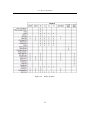
This system is complex and is basically composed by three different parts:
• Database: it stores data of all the athletes and trainers; most quantity of data are
originated by running computers and only a little quantity are inserted manually.
Other stored data are generated by software processing.
• Software +Atleta: it permits to the user to have a complete view of its training
data; they involve training plans, graphic and table views of numerous biological
parameters. These data can be analyzed and processed by the program. It manages
database connection and data storage.
• Running computer/external device: it provides the major part of input data. In
particular, it furnishes body parameters about each race or training session.
11
2 – Existing project
The following figure shows the system’s elements and the exchanged data flow:
Figure 2.2.
System’s elements
12
2.4 – Project description
2.4.1
Database
Existing database is composed by tables which contain the whole training system information. It is planned to store a great quantity of data. They are related to numerous
athletics teams, each one is composed by 20 athletes. Information could be personal data,
biological parameters and characteristics of every athlete and body data about all training
session or race done. Only topographic tracks information are not stored in the DB. This
is due to the fact that they are so many that it is not convenient to save them. In agreement
with the project manager, it is been decided to retrieve track information from external
file when it is needed to analyze them and not to store them into the local system. Finally,
the database is a MySQL DB [4], which provides all functionalities needed without any
license costs. It is accessed by using the MySQL++ library [13], described in the next
paragraph.
More in detail, the database structure is described by the following figure:
13
2 – Existing project
14
2.4 – Project description
Figure 2.3.
Database schema
15
2 – Existing project
MySQL++ library
MySQL++ is a powerful C++ wrapper for MySQL’s C API. It is built around STL (Standard Template Library) principles. MySQL++ helps the programmer to manage C data
structures, to generate easily repetitive SQL statements, and to manual creation of C++
data structures to mirror the database schema.
MySQL++ [5] has developed into a very complex and powerful library, with different
ways to perform a task. The purpose of this section is to provide an overview of the most
important used components of the library.
The process for using MySQL++ is similar to that of most other database access APIs:
1. to open the connection;
2. to form and execute the query;
3. to iterate through the result set.
Connection and query execution
Any connection to the MySQL server is managed at least by a Connection Object. The
most important function of the Connection is to create Query Objects for the user, which
are used to execute queries. The library also allows to execute queries directly through the
Connection Object, although the more powerful Query Object is strongly recommended
to execute queries.
To set up the Query Object to perform query executions there are three different ways:
1. standard Query Object is the recommended way of building and executing queries.
It is subclassed from std::stringstream, which means that it can be used
like any other C++ stream to form a query. The library includes also stream manipulators, which generate syntactically-correct SQL. This is the utilized method in
+Atleta system.
16
2.4 – Project description
2. Another useful instrument is the use of a Template Query. It works like the C
printf() function. The user sets up a fixed query string with tags inside, which
indicate where to insert the variable parts. This can be very useful in the case of
multiple queries that are structurally similar, because it is only necessary to set up
one template query, and use that in the various locations of the program.
3. A third method for building queries is to use Specialized SQL Structures (SSQLS).
This feature presents the results as a C++ data structure, instead of accessing the
data through MySQL++ intermediary classes. It also reduces the amount of embedded SQL code that a program needs. Unfortunately, a Visual Studio 2005 bug
does not allow users to utilize this method into the framework.
The field data in a result set are stored in a special std::string-like class called
ColData. This class has got conversion operators that let the programmer automatically
convert these objects to any of the basic C data types. Additionally, MySQL++ [4] defines
classes like DateTime, which can be initialized from a MySQL DATETIME string. These
automatic conversions are protected against bad conversions, and can either set a warning
flag or throw an exception.
As for the result sets as a whole, MySQL++ offers different ways of representing
them:
• Queries that do not return data. Not all SQL queries return data. An example is CREATE TABLE. For these types of queries, there is a special result type
(ResNSel) that simply reports the state resulting from the query: whether the query
was successful, how many rows it impacted (if any), etc.
• Queries that return data: dynamic method. The easiest way to retrieve data
from MySQL is using a Result object, which includes one or more Row objects.
Because these classes are std::vector-like containers, it is easy and powerful
to manage the result set as a two-dimensional array. For example, to obtain the
fifth item on the second row, what has to be typed is: result.at(1).at(4). It
17
2 – Existing project
also allowed the access to row elements by field name, like the following example:
result.at(2)[‘‘altitude’’]. An alternate way of accessing to the query
results is through a ResUse object. This class acts more like a Standard Template
Library input iterator than a container: programmers can analyze the retrieved result
set one item at a time, always going forward. This system has the disadvantage that
it is not possible to know how many results are in the set until the end is reached.
Finally, this method is more efficient when there are many results.
• Queries that return data: static method. Specialized SQL Structures (SSQLS)
define C++ structures that match table structures in the database schema. This is
called “static” method because table structure is fixed at compile time. If some
schema changes, update by programmer are required, to update its SSQLS definitions and recompile. In addition the program could crash or throw “bad conversion” exceptions when MySQL++ tries to stuff the new data into an outdated data
structure. The advantage of this method is that the program will require very little
embedded SQL code. By simply executing a query, results are received as C++ data
structures.
2.4.2
+Atleta software
+Atleta software has been developed by using the object oriented programming language
Visual C++ [1] and the Microsoft Visual Studio 2005 framework [6]. The implemented
application utilizes ActiveX components and the MFC (Microsoft Foundation Class) library. Its programming style follows the guidelines which were expressed in the previous
paragraph.
To understand the general software functioning, it is necessary to examine the following information:
• data organization: data are divided into three main categories, depending on their
function. They could be:
18
2.4 – Project description
– log: data from training computers. Each log is referred to a single training
session or to a single race. The whole original data set is visualized, and each
parameter has its own unit of measurement.
– Plan: it corresponds to a training model, which can be organized, created or
edited.
– Training Plan: it is a group of different plans, related to a single athlete.
• Function: at the moment, the following functions are available, which are grouped
by general thematic areas:
– security: data confidentiality is guaranteed by the initial login procedure that
asks the user’s name and password. Accounts can be created and subsequently
edited. There are two types of account: trainer or athlete. The trainer user can
manage personal and all training data (logs) about all the athletes of his team,
whereas athlete user can only see his owns. All the user data can be modified
or edited or cancelled in any moment.
– Calendar: by choosing a particular date, it is possible to get an association
with more than one Training Plan or simply more than one Plan.
– Log: it could be imported or exported, through the use of an XML file that
stores the data in a structured and fixed way. A log can be modified by the
athlete or by his trainer. It is allowed to know which plan is associated with
the log, to group more logs under a common root and to split a log in two or
more parts. In particular, this is a temporal division.
– Log comparison: it is possible to compare two different logs; the software
shows their parameters’ values: maximum, minimum and average value between them.
– Graphs: the software has lots of different graphic views. It has the goal to
show in the best way the training data of any log. It is possible to see only
some training data, not the whole data set. This is caused by the fact that
19
2 – Existing project
not all running computers store the same information. For example, +Atleta
shows parameters like heart frequency, altitude, speed and energy consumption, related to time or to the distance of the training route.
2.4.3
External devices
They represent the entry point for body parameters. Each runner who cooperates in the
development of this project, must have a training session using a running computer and
every time he/she must transfer data from the device to the PC, because device memory
is limited and probably cannot store more than one session’s data. In the initial part of the
thesis, researches have been operated in order to understand which body parameter could
be retrieved from an existing running computer. From a market research, it emerged
that there is a large number of running computer producers. In particular, what has been
stressed are three important companies which give good warranty about the quality of
their products. They are SUUNTO [3], POLAR [2] and GARMIN [1].
Web pages of these companies offer detailed information about technical specifications and features of each model. This made it possible to do a feature comparison between different models. In the following tables, what can be observed are the different
technical specifications relating to all the models of the three companies taken into consideration.
It is important to state that in this phase of the project development, not all sports are
considered, so we regard only models belong at the RUNNING category.
20
2.4 – Project description
Figure 2.4.
Suunto products
21
2 – Existing project
Figure 2.5.
Polar products
22
2.4 – Project description
Figure 2.6.
Garmin products
By examining the above tables, it can be noted that the most complete configuration,
which gives the major number of parameters, is composed by:
• heart monitor SUUNTO T6;
• SUUNTO foot POD;
• SUUNTO GPS POD;
• management software (SUUNTO training manager).
23
2 – Existing project
This equipment provides the user to receive data like heart frequency (maximum,
minimum and average), speed (maximum, minimum and average), times (plan, climb,
slide and lap), meteorological data (pressure and temperature), geographic data (altitude)
and thanks to the included software it permits to calculate/estimate other useful body
parameters including ventilation, oxygen consumption, respiratory rate, training effect
and EPOC (see glossary).
In general POLAR and SUUNTO instruments have similar and comparable features,
apart from the data analysis software; the SUUNTO’s one is more complex and elaborated
and for this reason it allows to perform a deeper and more useful data analysis.
GARMIN products are a little different compared to the previous ones. These are
more topography oriented and return high precision data about a training way, included
data like latitude and longitude, slide, climb and plan distances and times.
Missing data
Depending on the brand and model of the used training computer, some data cannot be
retrieved. This fact entails that +Atleta software can not have at its disposal all parameters, but only a part of them. In particular, only the parameters that they have in common
are stored into the database and can be analyzed. This work is focused to add on functionalities and capabilities to the +Atleta software, and to process and analyze these data.
To definitely complete this external device report, the following figures show which
are the missing data related on each brand:
24
2.4 – Project description
Figure 2.7.
Suunto missing data
As it has been previously written, SUUNTO T6 heart monitor is the most complete
device (only if used with GPS and foot POD). Models X6HR, X3HR and ADVISOR,
instead, do not produce data about calendar and training duration, while simpler models
like T4, T3 and TX do not provide any topography course data .
Figure 2.8.
Polar missing data
POLAR products are in general complete about body parameters, but RS100, RS200,
RS200SD, RS400 and RS400SD training computer do not allow at all to know information about track profile. RS800SD, RS800SD, S625X and S8101 have some data about
track profile, as for example altitude, but they do not provide particular details as GPS
coordinates.
25
2 – Existing project
Figure 2.9.
Garmin missing data
All GARMIN devices have installed a GPS so the exact profile of the training track
can be known. GARMIN software does not analyze deeply body data and does not furnish
estimated values of EPOC, VO2 and oxygen consumption. Therefore, low level products
as F101, F201 and F205 do not store any body data.
Finally, it is important to state that the market research has been made in April 2007,
during the initial phase of this thesis, and all the information about the mentioned parameters and device specifications are referred to this date.
Format file
POLAR, SUUNTO and GARMIN products generate data which are the point of departure
of the following analysis. Each company develops its own format file, which can be read
only by its own software product. In fact, when training session data are transferred from
the device to the PC, they are saved as a file. Subsequently, the software opens it and
shows the results to the user. More in particular, some details about the different format
files are reported:
• POLAR devices produce files with .hrm extension;
• GARMIN training computers generate files with .hst extension, or, with the new
versions .tcx one;
• SUUNTO heart monitors use .sdf extension.
26
2.4 – Project description
At the present time, the +Atleta software is not able to take on data directly from
devices, but the companies’ software have the feature to export their own logs in XML
format [7]. So +Atleta can import POLAR, SUUNTO and GARMIN logs thanks to its
implemented parsers. It is very important to note that each software has its own XML
format. Parsers are used to transform data from each XML file type to a standard XML
file used by +Atleta. This is an important feature of the software that reflects the aforesaid
project’s guidelines, in terms of using standard formal file for every producer. Furthermore, each XML file is different from the other one in terms of:
• kind of stored data;
• number of stored data;
• structural schema;
• precision degree of measurement;
• variable’s names;
• meaning of variable’s names.
It involves that is essential having an XML structured file equal for all devices. Moreover, it must contain the same information.
The facts just described represent a future works for +Atleta developers, because one
of the project’s guideline is to achieve the independency between the software and the
utilized training computer. So, at the moment, to import a log is necessary to follow these
steps:
1. transfer data from device to PC using its own company software;
2. export the selected file in XML format;
3. use +Atleta to standardize XML file and import it.
27
2 – Existing project
It is clear that all that has been just described represents a big fault of +Atleta. It must
be improved in the future, in order to achieve one of the main fixed points of this project:
the simplicity of use.
+Atleta XML format
The XML file has been studied and structured to contain all necessary information, which
will be subsequently analyzed, displayed and used to show a simulation of the run way
by the program. The file in question contains in addition data to build other files:
• HTML file to visualize data;
• WRL file to see the simulation track.
The XML file (see appendix B.1) shows the utilized structure to store data. The XML
schema is basically divided into three main labels, which are:
• Atleta: contains all personal data that describe the athlete and his/her physical characteristics; some of them are for example: sex, age, height and weight. Furthermore,
it contains maximum and minimum values of HR.
• DadesEntrenament: information about laps or parts of a single log (training session). In fact, a single log could be split into more laps. It stores data like speed,
distance, exercise type and atmospheric information.
• DadesEntrenamentHR: this section includes the main quantity of data, represented by sample data stored each instant; the sample’s number obviously depends
on the chosen sampling frequency.
28
Chapter 3
Statistical software
An important part of this thesis is focused on the creation of a structure able to perform
statistical data analysis. The MySQL database only provides simple descriptive statistics,
such as maximum, minimum and average value of stored data. In order to perform statistical analysis, it is necessary to use more powerful instruments. After researches, in
which all possible solutions have been studied, it has been decided to do not implement
any special C++ classes for this purpose, but to utilize an existing statistical software.
This approach is the result of the following considerations: to implement every statistical
function means to spend much time studying and deeply understanding the functioning
of every mathematical instrument that have to be used. Furthermore, there is a high
probability of error in development of algorithm calculations. On the contrary, statistical
software ensures reliability, a high precision level and provides a large number of simple
and complex functions. The last point represents a very important feature, because once
the structure has been created, it can be easily adapted and used to new and different statistical analysis. In terms of rapidity, simplicity, precision and future potentiality, to use
an existing statistical software guarantees a better result.
A large number of statistical software can be found on the market. In terms of precision level and reliability, there are not so many differences between products like SPSS,
MINITAB or R. If others factors are taken into account, the best software for the thesis’
purpose is R. It is the only one that has got some particular advantages: it is a free license
29
3 – Statistical software
and an open-source software, two characteristics that explain its continuous development
and improvement by its user community. In fact, R is the most used software by professors
and university researchers. Moreover R provides instruments to be remotely used by any
custom application. Finally, its simplicity of distribution and its extensive documentation
make it the most appropriate choice.
The goal of this chapter is to describe the infrastructure that has been created to embed R in +Atleta project. What has been created is the structure to perform the linear
regression of biological data stored into the database. This standard architecture has the
great advantage that it can be easily modified to perform all analysis that R allows and to
make full use of R capabilities.
3.1
R connectivity
As mentioned in chapter 2, one of the goals of +Atleta project is to create a simulation
model, to predict in advance athletes’ performances on a particular track. The starting
point can be represented by performing a linear regression, to predict a variable knowing
another one, using the statistical software R [8]. Obviously, linear regressions have to be
strongly embedded in +Atleta context. For this reason, R capabilities and characteristics
have been deeply analyzed. A great part of the work related to this thesis is focused on a
connection between +Atleta software and R.
R developers created a useful tool to connect R with any custom software; it is called
R SERVER. The goal in this chapter is to describe what R server is, how it has made
connections possible with others programs. Moreover, it aims at explaining which settings
and code lines on Visual C++ are needed to use R server under +Atleta. Considering
R server as a DCOM server which contains a COM-Interface to R, the first step is to
understand the general context and the meaning of these acronyms.
30
3.1 – R connectivity
Component Object Model (COM) is a platform for software components introduced
by Microsoft [5] in 1993. It is used to enable inter-process communication and dynamic
object creation in any programming language that supports this technology. The term
COM is often used in software development world as an “umbrella” term that encompasses the OLE, OLE Automation, ActiveX and COM+ technologies. The essence of
COM is a language-neutral way of implementing objects which can be used in different
environments from the one they were created in. For well-authored components, COM
allows reuse of objects with no knowledge of their internal implementation. This is due
to the fact that it forces component implementers to provide well-defined interfaces that
are separate from the implementation. The different allocation semantics of languages
are accommodated by making objects responsible for their own creation and destruction
through reference-counting. The preferred method of inheritance within COM is the creation of sub-objects to which method calls are delegated.
Distributed Component Object Model (DCOM) is also a Microsoft proprietary
technology for software components distributed across several networked computers to
communicate with each other. DCOM extends Microsoft’s COM, and provides the communication substrate under Microsoft’s COM+ application server infrastructure. DCOM
had to solve the problems of:
1. Marshalling: serializing and deserializing the arguments and return values of method
calls “over the wire”.
2. Distributed garbage collection: ensuring that references held by clients of interfaces are released when, for example, the client process has crashed, or the network
connection was lost.
31
3 – Statistical software
3.2
Embedding R in applications on MS Windows
As mentioned before, COM/DCOM objects define a standard for interoperability and their
function is assumed to be comparable with the one of a library. This kind of programming
technique, similar to the object-oriented paradigm, is more specifically called componentoriented. A component is fundamentally a basic unit that can encapsulate operations
(methods), data (properties) and state; it manages life-cycle by reference counting and
perform object creation.
It is important to know the right nomenclature:
• a component is called “COM/DCOM server”;
• a user of component is called “COM/DCOM client”.
The R SERVER package contains a DCOM server used to connect a client application
with R. As it was previously said, the R SERVER package provides a COM-Interface to
R as well as various COM objects and ActiveX controls do for many applications. R
(D)COM server has got a mechanism for:
• standard applications (like Microsoft Excel);
• custom applications written in any language to serve as a COM/DCOM client; they
use R as a powerful computational engine and renderer for graphics and text output.
After this general introduction, it is important to understand which the basic elements
that compose the R connectivity to +Atleta software are and in which way they are related.
The following figure shows the connections between R client, R server and R [11]:
32
3.2 – Embedding R in applications on MS Windows
Figure 3.1.
R connectivity structure
As can be observed from the picture above, the connection heart is R server, which
joins R1 and the software +Atleta. +Atleta represents a R client, and it can access to the
R engine only by R server. This last component controls and manages the access to R if
there are more clients at the same time.
In order to give a summary of what has been said before, main features of the package
R DCOM SERVER are the followings:
Use: thanks to the COM and DCOM technologies, it is possible to set R for local and
remote use respectively. DCOM allows transparent use of remote components and
application does not have to be changed for remote use. By paying attention to the
configuration settings on COM client’s and on COM server’s computer, it is possible to obtain user synchronization. To synchronize means that a given component
lives in a space that could be called “apartment” (comparable to thread context) and
execution context of a method call is always the component’s apartment. Into this
apartment, all method calls are synchronized, but it is not allowed to have parallel
1
It is required that R statistical software is installed on the computer.
33
3 – Statistical software
computations on a single R “instance”. In particular, this thesis’ work is focused
only on local use.
Data transfer: both from R to the client-application and vice versa, currently supporting
scalars (like booleans, integers, doubles and strings), arrays of these and arrays of
mixed data types (for example booleans and strings in a single array). Only one
array at a time can be past because the use of array of arrays is forbidden.
Text and graphics output: they are captured by using special ActiveX controls. They
allow to store outputs into particular data structures and subsequently import them
in the developed custom application.
Multiple local/remote server applications: the current implementation of the R server
package puts every single R interpreter used in a client application into a separate
address space. It also allows different code and data segments for multiple instances
of the interpreter even in a single client instance.
Multiple local/remote clients: using COM/DCOM to expose R’s functionality to client
applications even makes it possible to share a single instance of an R interpreter
between multiple client applications, both running on the same or even on different
machines in the network. Sharing an interpreter instance also implies a shared data
and code segment for R. The implementation using COM takes care of synchronizing access to the interpreter, so only one client can use the server’s functionality at
the same time.
34
3.2 – Embedding R in applications on MS Windows
Finally, it is important to state that clients and servers can communicate only using
COM/DCOM objects. COM/DCOM object is the media that allows communications and
data exchanges. It is composed by two parts:
• COM interface, which contains methods (functions and operations) and properties
(variables) visible by clients. It also contains its internal state, that is invisible by
clients. This interface represents the unique entry point to the object; an important
characteristic is that it must not be changed at all, even new methods cannot be
implemented. Given that it is an interface, it has an abstract definition and it is
identified by its IID (Interface IDentifier), a 128 bit numeric value.
• The second element is called Coclass, which is the implementation of COM interface. As many programming languages allow, even in this case, multiple Coclasses
can implement the same interface. Unlike the COM interface, the Coclass is identified by its CLSID (CLass IDentifier), a 128 bit numeric value or, more simply, by
its name. Coclass is referred to a COM client, who is programmed against interface,
and this reference is established at run-time.
3.2.1
Interface IStatConnector
IStatConnector interface is a COM interface that allows users to connect to R and exchange information with it. In fact IStatInterface defines the methods used to access to R.
Its structure is very simple, as the following example code shows. They are divided into
three thematic blocks:
35
3 – Statistical software
Figure 3.2.
IStatConnector interface
36
3.2 – Embedding R in applications on MS Windows
Referring to the code above, the following flowchart represents life-cycle of a COM
object that uses the IStatConnector interface:
Figure 3.3.
COM object life-cycle
37
3 – Statistical software
With the implementation of IstatConnector, it can be noted that all the components
involved assume a different role. On the one hand, R Server runs R in “background”,
it means that it is invisible by the user, while every objects gets its own process because
they have different symbol spaces in R server. R server also provides to redirect the R
graphic and textual outputs. On the other hand, R client runs R in “foreground” and user
can use R in parallel to many applications. Furthermore, every object accesses the same R
process, that is unique and allows one object access at a time, each one only in its shared
symbol space. In this context, textual and graphic output can be displayed in a window.
Finally, both Coclasses implement more COM interfaces and the application can use any
of them. Different CLSID are used in order to distinguish between them.
3.2.2
Data transfer
Unique allowed data transfer format is called VARIANT. The peculiarity of this format is
that it can contain any type of data, and this is determined by the VARIANT’s type (VT).
The main characteristics of VT are the followings:
• scalar values are supported. In particular:
– VT BOOL, VT I2, VT I4, VT UI1, VT R4, VT R8, VT BSTR;
– VT EMPTY;
– VT ERROR (xlErrDiv0, xlErrNA, xlErrNull).
• Arrays of same scalars of any dimensions represent the optimized data transfer
mode;
• arrays of different scalars generate the “mixed transfer mode”, who is not as efficient as the previous one.
COM Object can be transferred from application to R and vice versa. It simply utilizes
IStatInterface’s methods already described. Moreover, COM Object made possible to
send data and retrieve a particular operation or analysis on that. Furthermore, R text
38
3.2 – Embedding R in applications on MS Windows
output and R graphic output can be retrieved using two different ways, starting from the
fact that R (D)COM Server allows redirection of text and graphics output:
• Using ActiveX control for capturing text and graphic output available;
• Using COM object for (programmatically) capturing text output available.
In this project, the ActiveX approach has been used because it allows a greater simplicity of use and a more intuitive understanding. For this reason, additional functions
exist in IStatConnector Interface:
Figure 3.4.
Interface IStatConnector’s output
39
3 – Statistical software
3.2.3
Error handling
It is based on the assumption that every function returns an HRESULT result. For this
reason, standard COM error handling mechanism exist, which uses the macros SUCCEEDED() and FAILED() to check errors in functions. At the moment, it could be considered a great fault because the mechanism of error handling is not so easy and simply to
manage and utilize. The most effective example is that errors in every function call must
be checked. Anyway, to ensure the completeness, the following table quotes the most
common error codes:
Figure 3.5.
Error handling
40
3.3 – R connection example
3.3
R connection example
The following lines represent a sample C++ code that helps to immediately understand
what has been described until now:
41
3 – Statistical software
Figure 3.6.
42
Example
3.4 – Linear regression’s theory
A close examination of same passage is needed:
Figure 3.7.
3.4
Notes
Linear regression’s theory
As mentioned in chapter 2, one of the goals of +Atleta project is to create a simulation
model, in order to predict in advance athletes’ performances on a particular track. The
starting point can be represented by performing a linear regression, to predict a variable
knowing another one, by using the statistical software R. In this section, the linear regression’s theory is explained as well all passages that have to be followed to perform a linear
regression with R.
43
3 – Statistical software
Linear regression attempts to model the relationship between two variables by fitting a
linear equation to observed data. One variable is considered to be an explanatory variable,
the other is considered to be a dependent variable.
A linear regression line has an equation of this form:
y = mx + b
(3.1)
where
• x is the explanatory variable;
• y is the dependent variable;
• m is the slope of the line;
• b is the intercept (the value of y when x = 0).
Figure 3.8.
Linear regression line
The slope quantifies the steepness of the line. It equals the change in y for each unit
change in x. It is expressed in the units of the y-axis divided by the units of the x-axis. If
the slope is positive, y increases as x increases. If the slope is negative, y decreases as x
increases. The y intercept is the y value of the line when x equals zero and it defines the
elevation of the line.
44
3.4 – Linear regression’s theory
The goal of linear regression is to adjust the values of slope and intercept in order to
find the line that best predicts y from x. The most common method for fitting a regression
line is the method of least-squares.
More precisely, this method calculates the best-fitting line for the observed data by
minimizing the sum of the squares of the vertical deviations from each data point to the
line (if a point exactly lies on the fitted line, then its vertical deviation is 0). Since the
deviations are first squared, then summed, there are no cancellations between positive
and negative values.
In order to better understand the working of this method, in this page are reported the
formulas that have to be used to perform a statistical treatment to the data. Given a set of
data (xi ,yi ) with n data points, the slope (m) and y-intercept (b) can be determined using
step by step the following formulas:
x average value:
n
1X
xi
n i=1
(3.2)
n
1X
yi
µy =
n i=1
(3.3)
µx =
y average value:
V AR(x):
σx2
n
1X
=
(x2i − µ2x )
n i=1
(3.4)
n
1X
(yi2 − µ2y )
n i=1
(3.5)
n
1X
[(xi yi ) − (µx µy )]
n i=1
(3.6)
V AR(y):
σy2 =
COV (x,y):
σxy =
45
3 – Statistical software
Correlation coefficient:
σxy
σx σy
(3.7)
σxy
COV (x,y)
= 2
V AR(x)
σx
(3.8)
rxy =
Slope:
m=
y-intercept:
b = µy − mµx
(3.9)
Note that linear regression does not test whether the data are linear. It assumes that
data are linear, and finds the slope and intercept that make a straight line which best
fit the data. For this reason, it is necessary to find parameters which give a measure
of correctness of fit of linear regression. A valuable numerical measure of association
between two variables is the correlation coefficient, rxy . It is a value between -1 and 1
indicating the strength of the association of the observed data for the two variables. The
correlation coefficient, gives a measure of the reliability of the linear relationship between
the x and y values. A value of rxy = 1 indicates an exact linear relationship between x and
y. Values of rxy close to 1 indicate excellent linear reliability. If the correlation coefficient
is relatively far away from 1, the predictions based on the linear relationship, y = mx + b,
will be less reliable. Some examples are present in the next page.
46
3.4 – Linear regression’s theory
Figure 3.9.
Correlation coefficient
There is another parameter that functions exactly as the correlation coefficient. It is
called coefficient of determination and its symbol is r2 . In the simple linear regression
it is the square of the correlation coefficient. The value r2 is a fraction between 0.0 and
1.0, and has no units. An r2 value of 0.0 means that knowing x does not help to predict
y. There is no linear relationship between x and y, and the best-fit line is a horizontal line
going through the mean of all y values. When r2 equals 1.0, all points lie exactly on a
straight line with no scatter. Knowing x let predict y perfectly. For example, a r2 value of
47
3 – Statistical software
0.726 indicates that 72.6% of the variation in one variable may be explained by the other.
Finally, it is very important to remember that the absence of linear relationship between variables does not mean that any relationship between them does not exist.
3.5
Linear regression using R
Modern statistical software can execute steps described in the previous paragraph automatically, performing calculation in few instants. In particular, by using the statistical
software R, a linear regression can be performed following these few passages [12]:
1. data set declaration: each data set has to be filled in vectorial form;
2. linear regression command: using the command lm, it is possible to perform the
linear regression between variables;
3. data set display: typing plot it is possible to obtain a graphic representation (scatterplot) of the used data set;
4. fitting line display: the abline command is used to display the calculated fitting
line;
5. show results: the summary command is useful to show all information about the
linear regression just performed.
The following example is useful to understand immediately previous points:
48
3.5 – Linear regression using R
Given the data set (x,y), R produces two kinds of output:
1. Graphic output: it is composed by the scatterplot of the data set and the fitting line.
Figure 3.10.
R graphic output
2. Textual output:
49
3 – Statistical software
As can be observed, the textual output is composed by numerous lines, each one
containing statistic information and estimated parameters. In particular, there are two
values that assume great importance to verify the correctness of the used method:
• Multiple R-Squared: already described, also called coefficient of determination,
it represents a valuable numerical measure of association between variables;
• P-value: in statistical hypothesis testing, is the probability of obtaining a result at
least as extreme as a given data point, under the null hypothesis. The fact that pvalues are based on this assumption is crucial to their correct interpretation. It is a
probability, so its value is a fraction between 0.0 and 1.0.
It has been introduced a new term: the null hypothesis [6]. It is a hypothesis set up
to be nullified or refuted in order to support an alternate hypothesis. When used, the
null hypothesis is presumed true until statistical evidence in the form of a hypothesis test
indicates otherwise. This means that the null hypothesis proposes something initially
presumed true. It is rejected only when it becomes evidently false. That is, when one has
a certain degree of confidence, usually 95% to 99%, the data does not support the null
hypothesis.
Formulation of the null hypothesis is a vital step in testing statistical significance.
Having formulated such a hypothesis, the probability of observing the obtained data or
data more different can be established from the prediction of the null hypothesis, if the
null hypothesis is true. That probability is what is commonly called significance level
of the results. Generally, one rejects the null hypothesis if the p-value is smaller than or
equal to the significance level. In this case, the null hypothesis is formulated when the
method of least-squares is applied.
Given the model in the following form:
yi = β0 + β1 xi
50
(3.10)
3.5 – Linear regression using R
As aforesaid, the aim of this method is to calculate the values of β0 and β1 that minimize:
n
X
(yi − β0 − β1 xi )2
(3.11)
i=1
The null hypothesis is:
H0 : β1 = 0
(3.12)
It follows that the alternate hypothesis is:
H1 : β1 6= 0
(3.13)
Calling α the significance level, it is possible to have only two scenarios:
if α < p value
H0 is accepted
if α > p value
H0 is rejected
Normally, if H0 is rejected, the linear regression fits the given data set.
Final clarifications are needed because there are several common misunderstandings
about p-value. Here the most frequents are reported:
1. The p-value is not the probability that the null hypothesis is true (claimed to justify
the “rule” of considering as significant p-values closer to 0). In fact, it is not possible
to attach probabilities to hypotheses.
2. The p-value is not the probability of falsely rejecting the null hypothesis.
3. The p-value is not the probability that a replicating experiment would not yield the
same conclusion.
4. 1-(p-value) is not the probability of the alternative hypothesis being true.
51
3 – Statistical software
5. The significance level of the test is not determined by the p-value. The significance
level of a test is a value that should be decided upon by the agent interpreting the
data before the data are viewed. It is compared against the p-value or any other
statistic calculated after the test has been performed.
6. The p-value does not indicate the size or importance of the observed effect.
Finally, in appendix B.3 is present the programming code of +Atleta that performs
the linear regression of two variables by using R and that shows R’s graphic and textual
outputs.
3.6
Biomedical motivations
At the moment, in +Atleta software only few linear regressions have been performed.
The following lines explain the motivations and the information that can be retrieved
from them [14]:
1. HR - SPEED: it represents one of the most important factors. In fact, the knowledge
of the relation between HR and speed is very important to estimate the athletic
training level of a person. Observing this parameter, it is possible to know if it is
necessary to modify current training sessions to improve the athlete’s performance
or not. For example, to have a high speed and a relatively low HR is index of a great
athletic training level. This is due to the fact that it means that the athlete can run
faster with a lower energy consumption.
2. HR - ALTITUDE: a factor that can be observed is the body altitude adaptability. At
high altitude (about 2000 m) to do physical activity is more exertive; this is due to
the decreasing of oxygen concentration in the air. Less oxygen availability usually
entails the increasing of HR and respiration rate, too. This is the body natural
behavior to maintain a constant level of oxygen in the system for a short period.
Another typical body reaction (usually at higher altitudes, over 2000 m) is the red
blood cell increasing, to transport more oxygen quantity.
52
3.6 – Biomedical motivations
3. HR - DISTANCE: its progress indicates if an athlete is trained enough to large
distances. This is a secondary factor compared to the first ones, but, anyway, it
represents an aspect that does not have to be forgotten. For example, if the athlete’s
HR significantly increases after a certain covered distance, this could imply wrong
training plans for long distances.
4. SPEED - ALTITUDE: this parameter is very similar to the HR - ALTITUDE one,
described at the point 2. This is due to the fact that maintaining a high speed on
a high altitude entails a stronger HR increasing than at lower altitudes. A very
interesting analysis could be to compare performances at different altitudes (with a
significant gap), and to observe the speed variations in both cases.
5. SPEED - ENERGY: this factor relates speed and energy consumption. It assumes
significance only if it is associated with HR, DISTANCE and GRADIENT values. It
is very particular, because it does not give a physical parameter, but a psychological
one. It signals if a runner feels at ease running to a certain speed or not. It happens
that some athlete prefers run at low speed, also for very long distances; others, for
example, do not feel at ease running fast on a slope or they spend too much energy
on a climb. In all these cases, energy consumption value changes.
6. SPEED - DISTANCE: this data has to be associated to the HR - DISTANCE analysis [15]. It indicates the body behavior, especially on long distances. It can be
interesting to understand if a runner knows how to manage a long distance race,
rationing his/her forces and energy to maintain a constant performance or not.
53
Chapter 4
Analysis algorithms
4.1
Exertion algorithm
In order to be effective and to cause an adaptable response, a training session must in
some way cause disturbance in the body’s internal balance. This particular phenomenon
is called “homeostasis”. Any physical exercise per se is exertive and deteriorates performance, but after training, during the recovery phase, the body is being “built up”. The
body adapts to the requirements of exercise in order to be able to perform that task again.
Actually, the body is “built up” a little better than it was before, a phenomenon known as
“supercompensation”.
To know the supercompensation level and the right training frequency, it is important
to estimate how exertive are training sessions. The method which has been utilized in
this thesis in order to calculate exertion, is the same suggested in the POLAR Precision
Performance software manual [2].
Another important factor to consider is the time required for recovery. It foremost depends on the intensity (HR) of the training session and also on the duration of this session.
For athletic training, it is essential to schedule training sessions at correct intervals: not
too close to each other in order to avoid overtraining and not too far from each other in order to avoid undertraining. However, it is difficult to evaluate the effects of both intensity
55
4 – Analysis algorithms
and duration in respect of the recovery time needed. Until now, it has been difficult to estimate the time needed for recovery after training sessions when athletic training consists
of several different types of training.
Figure 4.1. A schematic presentation of the acute effects of an exercise bout on
performance. The vertical axis depicts the intensity and the horizontal axis shows
the duration of an exercise
As can be seen from the previous schema, the immediate effect of an exercise is a
decrease in the performance level. After the exercise, a recovery phase occurs and the
performance curve slightly rises above the initial level. This phenomenon is exactly the
supercompensation. Thus, for a short and certain period of time after the exercise session, the performance improves to a level slightly higher than it was before that exercise
session. This phenomenon is the basis of all training programs. The next training session
should occur during the supercompensation phase. Then, it is possible to gradually increase performance, starting each time from a slightly higher level. However, if the next
exercise comes too early, the performance level will decline even more, and the recovery
will take longer. Respectively, if the next session is delayed, and is done when the supercompensation phase is over, the net effect of multiple sessions will be close to zero.
The exertion count is designed to make all exercise sessions measurable referring to sport,
duration and intensity level.
As mentioned before, the most useful information from the exertion count comes
when one learns to relate his/her exertion level to the time needed for recovery after a
single training session. The figure in the next page shows a schematic view of the suggestive relationship between exertion and recovery time. The values used are personalized.
56
4.1 – Exertion algorithm
Therefore, a record of his/her own experiences and findings should be kept for several
weeks before applying this analysis.
Figure 4.2.
A schematic relationship between exertion count and recovery time
The previous figure shows, for example, that for a exertion value of about 300, the
related recovery time is of about one day. Past this time, the athlete is able to perform
a new training session, because his/her body is in the supercompensation phase. When
one has found out how his/her own exertion factors relate to recovery, he/she can easily
control his/her training in advance. It is also possible to know after each session when
he/she is able to start the next one. The exertion count rapidly reveals when easy days
have come and if the load has been constant or inconstant.
The heart rate level achieved during light recovery exercises accurately demonstrates
the body’s exertion level. When recovery has been unsuccessful, the heart rate tends
to rise and speed to decrease. In addition to heart rate and speed, subjective feelings
during the exercise are also an essential part of evaluating the exertion level. All three
variables - heart rate, speed and feelings - describe the exertion level. Sometimes changes
are apparent in only one of the above factors. When heart rate, speed and feelings are
regularly monitored during light and recovery exercises, the athlete is able to immediately
react to changes in the above factors. This ensures optimal development and helps to avoid
overexertion. The graph in the next page can be observed in order to clarify this concept.
The graph compares two exercises performed in two different states of recovery. The
57
4 – Analysis algorithms
objective of the exercises has been to perform a steady-paced light run. Moreover, the
exercises have been performed in the same place. The lower heart rate curve corresponds
to an exercise performed after proper recovery. The athlete’s subjective feeling has been
good. The average heart rate is 127 bpm and speed 4.26 min/km. The upper heart rate
curve corresponds to an exercise that was felt to be difficult. The average heart rate is 137
bpm and speed 4.30 min/km. The heart rate curves show a distinct difference in the state
of recovery. The situation demonstrated by the upper curve is due to heavy training during
the days prior to the test. It is important to state that increased heart rate level during light
aerobic training may also be caused by other factors, such as flu.
Figure 4.3.
4.1.1
Heart rate curves comparing recovered situation vs. strained/tired situation
Calculating the exertion count
The exertion count has been developed to ease and simplify the analysis of athletic training programs. It combines three factors of a training session into a single measurable
figure:
1. duration (time, expressed in minute);
58
4.1 – Exertion algorithm
2. intensity (heart rate, expressed in beats per minute);
3. sport factor (constant depending on the sport).
For each training intensity interval (HR interval), is given an exertion factor by which
the time spent at that HR is multiplied. Some exercise modes or sports have their additional impact on the exertion and thus a sport factor is applied. The exertion count is the
total sum of these three components. Its formula is the following one:
Exertion =
n
X
[(EF of HR interval) · (time spent in that interval)] · (SF ) (4.1)
i=0
where:
• EF is the Exertion Factor;
• SF is the Sport Factor;
• i is the index of the HR interval;
• n is the number of HR intervals.
The concept of exertion count is easy to understand with the help of the chart of the
next page. The chart describes relative exertion as a function of exercise heart rate. The
higher the heart rate, the harder is the exercise. It is easy to agree that 30 minutes of
exercise at HR of 160 beats/min is about twice as exertive as 30 minutes at HR of 140
beats/min. The exertion count is a simple way to express the total exertion of a single
training session as a combination of the intensity and duration of exercise. The exertion
count values are typically from 50 - 400. At these magnitudes, they are easy to use in
simple calculations.
59
4 – Analysis algorithms
Figure 4.4.
The relative exertion of an exercise as a function of heart rate
A last consideration has to be done about sport factors. The definition of sport factors is targeted at an advanced user of the software. As can be seen from the following
statements, several factors are involved when determining an appropriate factor for a certain sport. The basic assumption is that each individual has his/her favorite sport which
is most often used. The following presents a selection of the most popular sports and
recommendations for their sport factors. The recommended factors range within 0.8-1.3,
thus being of relatively minor importance, and therefore emphasize the importance of HR
measurement in all training sessions.
Running/jogging 1.0
Running is expected to be the most common sport, and thus has the factor 1.0 to
which other sports are related.
Aerobics 0.9-1.1
The correct factor of aerobics depends very much on the type of a particular program. Typically aerobics consists mainly of dynamic movements mainly involving
lower extremity muscles. Also, the recovery phases, if there are any, are relatively
short. The differences between step/low/high/combo are mainly reflected in HR.
60
4.1 – Exertion algorithm
Cycling 1.1-1.2
To reach the same HRs, one will have to work approximately 10 to 15% harder
in cycling than in running. That is mainly due to the slightly slower frequency
of cycling, the lack of a weight bearing task in cycling and the larger amount of
eccentric work in running.
Mountain biking 1.0-1.1
Mountain biking differs from road cycling as regards the usage of upper body muscles and the amount of standing. Also, the varying terrain makes the demands of
mountain biking somewhat higher than those of road cycling but mostly these differences are also reflected in the HR.
Stepping 1.0-1.2
As to the sport factor, stepping is very much like cycling, as it lacks the eccentric
component of work, yet requires a relatively large muscle mass. However, the
rhythm of work may impair circulation and thus cause an increase in blood lactate.
This, in turn, may not be reflected in the HR and should therefore be taken into
account in the sport factors.
Canoeing, paddling 1.2-1.3
This is a typical upper body exercise. For an occasional canoeist high HRs are
difficult to reach, but the upper body may be rather exhausted, because the work is
done by a limited muscle mass.
Rowing 0.9-1.2
See cycling and stepping. However, the involvement of upper body may cause
effects such as in cross-country skiing.
61
4 – Analysis algorithms
Walking 1.1
Walking is similar to biking in regards to the effort for reaching a given HR. Again,
this is due to the mainly concentric work of muscles. Also walking lacks the rapid
and large limb movements which per se increase HR.
Swimming 1.2-1.3
For a recreational swimmer high HRs are difficult to reach, giving swimming a
high factor. The respiratory muscles are highly stressed, which is also the case with
upper body and hip muscles.
Tennis 1.0
Tennis is a game in which rapid movements and the work of the whole body are
combined with relatively long pauses. This combination allows your HR to react
quite precisely so that additional factors may not be needed.
Badminton 1.1-1.2
The abrupt nature of badminton makes your HR rise relatively easily. However, the
energy production lies mainly on carbohydrates and anaerobic energy yield without
adequate respiratory stimulus, and leads into a slight underestimation of exertion if
based solely on HR.
Squash 1.0-1.1
Squash is similar to badminton by nature, yet a lower factor is recommended because the movements are shorter than in badminton.
Soccer 1.0
See tennis. The demands of soccer depend greatly on the player’s role.
62
4.1 – Exertion algorithm
Skating 1.1-1.2
In line skating resembles cycling but the resting periods are longer (step frequency
is very low). On the other hand, there is a long static phase during each step which
makes the sport rather heavy.
Cross-country skiing: classic 0.9
It is possible to reach the same HR somewhat easier in whole-body work, but also
the total energy expenditure will be a little more on a given HR than in running.
Cross-country skiing: freestyle 1.1-1.2
Skating or freestyle skiing very much resembles skating, yet the HR is lower than in
the classic style mainly because of long static phases and relatively slow movements
and frequency in the upper body.
These examples refer only to normal conditions, and are not applicable to extremely
long or exhaustive exercise sessions. These factors are valid only together with HR data.
It cannot be stated that 1 hour of biking is 10% harder than 1 hour running. The question
should rather be put in this way: “Is it harder to run at HR of 150 beats/min than to cycle
at the same HR?”.
4.1.2
The algorithm
Using the aforesaid formula and method, the exertion algorithm has been implemented.
Its functioning is very simple: for each existing HR interval, it multiplies the related
exertion factor (chosen with relation to the figure 4.4) per time spent in that HR interval.
Then, the algorithm sums all these values and applies the related sport factor.
Finally, it is important to notice that, if there is more than one training session in a
day, the algorithm calculates the daily exertion count as sum of all the exertion counts of
each training session.
63
4 – Analysis algorithms
The implemented exertion algorithm is described in detail by the following pseudocode:
1 initialize total exertion value of a log at 0
2 execute cycle for all logs of a single day
2.1 initialize partial HR interval exertion at 0
2.2 execute cycle for all athlete’s HR intervals
2.2.1 retrieve seconds, minutes and hours spent in this HR interval
2.2.2 transform all in minutes: multiply hours spent per 60
2.2.3 transform all in minutes: divide seconds spent per 60
2.2.4 sum of transformed seconds and transformed hours and minutes
2.2.5 multiply total time spent per related exertion factor
2.2.6 add the calculated partial HR interval exertion (i) to the previous one
(i-1)
2.3 multiply the total exertion value of a log per the related sport factor
2.4 add the calculated total exertion value of a log (i) to the previous one (i-1)
4.2
Gradient algorithm
It is very important to know the athlete’s performance respect to the altitude development
of a track. In fact, athletes could have significant difference in terms of speed or energy
consumption depending on the ground slope. For example, an athlete could have a great
resistance in a climb, but not have a good running technique during slopes, so his/her
performances can be affected by these factors. Studying track profiles related on training
session is useful to highlight body limits or athletic faults, to perform the best training
sessions to improve athletes performances.
Starting from the punctual values of distance and altitude, represented on the x-axis
and y-axis of a Cartesian graph respectively, this algorithm has the goal to show a different
track profile. It associates to a single line segment more sub-segments which have in
common the similar gradient value. This is important to obtain a less jagged track profile,
which can be studied and analyzed with much more simplicity. From it, one can see lots
64
4.2 – Gradient algorithm
of information about track gradient in different parts of the track, like for example HR,
speed and energy consumption variation in relation with their own gradient values.
The gradient algorithm utilizes the line segment interpolation to calculate in a easy
way the gradient value. Obviously exist lots of algorithms to interpolate points, but the
undersigned uses the line segment because:
• it is the simplest one;
• it does not introduce noise in calculation;
• it is not possible to know the exact track profile between two points, so it is impossible to establish which algorithm is the best one;
• modifying the angular limit, it is possible to obtain many precision levels.
The algorithm idea is that a point belongs to a certain line segment, if the gradient of
the segment line delimited by the same point and the previous one, respect to the average
gradient value of the line segment, does not exceed a calculated threshold (expressed in
terms of decimal degrees). This is the basic idea of the gradient algorithm, that functions
very well if the track has steep climbs or large slopes, exactly as shown in the following
picture:
Figure 4.5.
Climbs and slopes
65
4 – Analysis algorithms
The decision threshold allows that there will be a little angular margin between two
different gradient values, both in slope and in climb. For this reason, it is possible to
obtain profiles like the following one:
Figure 4.6.
Gradient view
Moreover, a last consideration has to be made. In reality, lots of tracks have a different
profile in terms of altitude. For example, mountain roads, with lot of ups and downs
can be easily imagined. For this reason, the original idea has been improved: not only
one point has been involved in the calculation, but also its two following points. This
improvement is useful because the algorithm does not only consider one point respect
to the line segment gradient, but also the future progression of the track profile. In this
way it is possible to avoid and to do not consider little oscillations of the profile or wrong
altitude values. The following picture is an example of this behavior:
66
4.2 – Gradient algorithm
Figure 4.7.
Possible wrong value
It is necessary now to describe how the algorithm works, scanning each point of the
track profile. It involves in its calculation four points at a time: the current scanned point,
the previous point and the two following ones. It starts calculating the fictitious gradient
value of the three different line segments delimited by the mentioned points:
• the first is delimited by the current point and the previous one;
• the second is delimited by the next point of the current point and the previous one;
• the third is delimited by the second next point and the previous one.
67
4 – Analysis algorithms
Figure 4.8. Involved points in gradient algorithm
In the picture, the scanned point is marked as “i”, the previous point “i-1” and the
following ones “i+1” and “i+2”. Intuitively, the line segments’ names are “s1”, “s+1”
and “s+2” respectively. Furthermore, it is important to state that in the gradient calculation, the distance between two points has been intended as horizontal distance and not
as inclined one. Since the majority of distance data are originated by GPS devices, the
undersigned has utilized the topographic approach that works in this way. In addition, the
difference between the two distances is so little that can be assumed as nonessential, and
the precision of the calculation is not affected by errors. The gradient is expressed by the
α angle of a right-angled triangle, as shown:
68
4.2 – Gradient algorithm
Figure 4.9.
Right-angled triangle
Using the trigonometry law, the formula for α angle is the following:
"
b
α = arctan
a
!#
(4.2)
And it follows that the formula for gradient is:
"
α
rad
altitude
= arctan
distance
!#
(4.3)
The C++ programming language offers a library to developers, math.h, which contains lot of mathematics functions [2]. The formula for gradient which has been used in
this project, has been lightly modified because math.h can only manage radiant angles,
but to be more user-friendly, the +Atleta interface show only decimal degrees. The final
formula for gradient calculation is:
"
altitude
α = arctan
distance
◦
!#
·
180
π
(4.4)
Once the three fictitious gradient values are calculated, the algorithm updates the value
of the current general line segment gradient. It is calculated as average of all the sub-line
segment gradients, which are composing (at the moment) the questioned line segment.
The algorithm operates a comparison between it and the evaluated fictitious gradients
calculated in advance. This comparison establishes if the current point (i) could be part of
69
4 – Analysis algorithms
the current line segment. The “i+1” and “i+2” points represent the future development of
the track, and for this reason assume a great importance in this decision. They can avoid
errors due to little track oscillations or wrong stored altitude values. It is also important to
notice that an angular threshold exists (defined and configured by users) to perform this
comparison. The “i” point belong to the line segment if one of the following conditions
is satisfied:
• if gradient of “s1” does not exceed the angular threshold;
• if gradient of “s2” does not exceed the angular threshold;
• if gradient of “s3” does not exceed the angular threshold.
Observing this rule, it is easy to notice that “i” point does not belong to the line
segment only in the case that all three fictitious gradients exceed the angular threshold.
For this reason, different scenarios could be presented:
1. current point belong to the line segment because “i” point does not exceed the angular threshold
Figure 4.10.
70
Case 1
4.2 – Gradient algorithm
2. current point belong to the line segment because “i+1” point does not exceed the
angular threshold. In this case “i” altitude exceed the angular threshold, but the algorithm considers more important the future track trend. This altitude is rejected: it
can be considered as a wrong value which is due to device errors. Here an example:
Figure 4.11.
Case 2, graph view
The shown graph could be represented in this way:
Figure 4.12.
Case 2, schematic view
71
4 – Analysis algorithms
3. current point belong to the line segment because “i+2” point does not exceed the
angular threshold. This case is similar to the previous one, but there are two values
that are out of scope. Next picture will show an example.
Figure 4.13.
Case 3, graph view
The shown graph could be represented in this way:
Figure 4.14.
Case 3, schematic view
72
4.2 – Gradient algorithm
4.2.1
The algorithm
In order to summarize what has been described until now, it can be said that the algorithm
works in the following way: before deciding if a point could be part of a certain line
segment, three tests are performed. They check if all the three next points (of the point
considered in a certain moment) could be part of the line segment. This happens comparing the average gradient of the general line segment and the three gradients of the line
segments, i.e. segments obtained joining the points “i”, “i+1” and “i+2” with the point
“i-1”. It is necessary that at least one of the three tests is past, to consider the “i” point as
part of the general line segment. In this way, all points belonging to the track are checked,
not simply testing their positions, but also keeping the future track trend into account.
The detailed gradient algorithm is described by the following pseudo-code:
1 execute cycle from 1st element to third last element of punctualData vector
1.1 if previous point (i-1) is the starting point of the track
1.1.1 calculate the gradient of the segment delimited by it (i-1) and current
point (i)
1.2 else segment’s gradient value already exists
1.2.1 update it calculating new average segment’s gradient (segmentGradient)
1.3 retrieve relative distance and relative altitude between current point (i) and previous point (i-1)
1.4 calculate gradient of the segment delimited by current point (i) and previous
point (i-1)
1.5 retrieve relative distance and relative altitude between next point (i+1) and previous point (i-1)
1.6 calculate gradient of the segment delimited by next point (i+1) and previous
point (i-1)
1.7 retrieve relative distance and relative altitude between second point (i+2) and
previous point (i-1)
73
4 – Analysis algorithms
1.8 calculate gradient of the segment delimited by second next point (i+2) and
previous point (i-1)
1.9 calculate tolerance range, the maximum (maxRange) and minimum (minRange) angular limit as sum/subtraction of segmentGradient and gradientFactor
1.10 perform a three level tolerance control: if gradient calculated at (1.4) exceeds the tolerance range
1.10.1 if gradient calculated at (1.6) exceeds the tolerance range
1.10.1.1 if gradient calculated at (1.8) exceeds the tolerance range
1.10.1.1.1 current point is not part of previous line segment because
it is out of range
1.10.1.1.2 store data related to previous line segment. It goes from
starting point to (i-1) point
1.10.1.1.3 set previous point as the new starting point
1.11 return at the cycle start (1)
2 update mean segment’s gradient (segmentGradient)
3 retrieve relative distance and relative altitude between current point (i) and previous
point (i-1)
4 calculate gradient of the segment delimited by current point (i) and previous point
(i-1)
5 retrieve relative distance and relative altitude between next point (i+1) and previous
point (i-1)
6 calculate gradient of the segment delimited by next point (i+1) and previous point
(i-1)
7 calculate tolerance range, the maximum (maxRange) and minimum (minRange) angular limit as sum/subtraction of segmentGradient and gradientFactor
8 perform a two level tolerance control: if gradient calculated at (4) exceeds the tolerance range
8.1 if gradient calculated at (6) exceeds the tolerance range
8.1.1 current point is not part of previous line segment because it is out of
range
8.1.2 store data related to previous line segment. It goes from starting point
to (i-1) point
74
4.2 – Gradient algorithm
8.1.3 set previous point as the new starting point
9 update mean segment’s gradient (segmentGradient)
10 retrieve relative distance and relative altitude between current point (i) and previous
point (i-1)
11 calculate gradient of the segment delimited by current point (i) and previous point
(i-1)
12 calculate tolerance range, the maximum (maxRange) and minimum (minRange) angular limit as sum/subtraction of segmentGradient and gradientFactor
13 perform a single level tolerance control: if gradient calculated at (11) exceeds the
tolerance range
13.1 last track point (current point) is not part of previous line segment because it
is out of range
13.2 store data related to previous line segment. It goes from starting point to (i-1)
point
13.3 set previous point as the new starting point
13.4 store data related to the last line segment. It goes from previous point (i-1)
point to current and last track point
14 else last track point (current point) is part of previous line segment (last track line
segment)
14.1 store data related to last line segment. It goes from starting point to the track
final point
75
4 – Analysis algorithms
4.3
Bend algorithm
Starting from the simple topographic coordinates, this algorithm has the purpose to detect
when there is a bend in the track and if it is a left bend or a right one. It is important
to know these circumstances because each runner has his own run technique that very
much depends on his preferred leg, i.e. a leg more powerful than another. The fact that
each athlete has got a preferred leg, could entail differences in term of speed and energy
consumption and could concern a left or a right bend. For this reason, to cover a track
in a way or in the opposite one, could involve that the same athlete can obtain different
performances. This behaviour has been acutely taken into consideration, studied and
analyzed.
The idea of this algorithm is that a track is represented by a sequence of line segment.
Track data are GPS coordinates which can be displayed by using a simple Cartesian graph.
Depending on the amplitude of the calculated angle between each adjacent line segment,
the following cases can be presented:
• if the angle value is too high, compared to a fixed threshold, there is no bend. The
reason is that the two line segment compose nearly a straight line;
• if the angle is under the threshold there are different scenarios:
– there is a bend if the previous bend is too far (respect to the fixed “distance
threshold”) or if the previous one is on the opposite side;
– there is not a new bend, because this one is already part of a greater bend.
Therefore, this algorithm establishes these different scenarios and it detects in which
one the analyzed line segment is in. Then, it stores parameters like mean HR, speed,
energy consumption and gradient of each bends. It is important to notice that, if a bend
is composed by more than two line segments, the algorithm provides for the average
calculation of the aforesaid parameters. Moreover, it does an average among all the line
segments involved.
76
4.3 – Bend algorithm
The first step consists on a transformation of a line segment, expressed by the Cartesian coordinates of its extreme points, into a line segment expressed by polar coordinates.
Polar coordinates are the length (s) and the angle (α).
Figure 4.15.
Point’s representations
In order to do this, it is useful to apply the Pythagorean theorem, and to calculate the
”s” line segment as the hypotenuse of a right-angled triangle. It is shown by the following
picture:
77
4 – Analysis algorithms
Figure 4.16.
Right-angled triangle
The formula is:
s=
q
(xB − xA )2 + (yB − yA )2
(4.5)
The fundamental aspect to continue in the bend calculation is to obtain the polar length
of each adjacent line segments. The following step is to calculate the angle between them.
To reach this goal it is necessary to use Carnot’s theorem. It states the following relations
between sides and angles and could be applied to any triangle:
a2 = b2 + c2 − 2 · b · c · cos α
(4.6)
b2 = a2 + c2 − 2 · a · c · cos β
(4.7)
78
4.3 – Bend algorithm
c2 = b2 + a2 − 2 · b · a · cos γ
Figure 4.17.
(4.8)
Carnot’s triangle
In the case of a track, considering two line segment at a time, the triangle could appear
in this form:
Figure 4.18.
Bend angle
Moreover, once the sides of the triangle have been calculated with the 4.5 formula (as
shown in the picture, they are the real line segments “a” and “b” and the fictitious one
79
4 – Analysis algorithms
“c”), with the inversion of the formula 4.8, it is easy to find the γ angle, i.e. the bend
angle:
b2 + a2 − c2
γ = arccos
2·a·b
!
(4.9)
The next step is more complicated. It has the goal to determine if the bend is on the
right or on the left side. In order to do this, it is necessary operate a roto-translation of the
Cartesian axis. This operation has to be done for each bend and is the way to determine
the following bend’s side. Particularly, the x-axis is superimposed to the analyzed line
segment and its direction is the same of the track’s one. The following example will
better clarify this concept:
Figure 4.19.
Axis’ standard configuration
80
4.3 – Bend algorithm
Figure 4.20.
Axes’ roto-translation
With this new axis’s configuration, the new axis origin is represented by point “A” and
x-axis is superimposed to the first line segment “s1”. In this way, the only coordinates that
have to be estimated are related to point “C”. In order to calculate them, it is necessary to
use the following formulas:
0
xC = (xC − xA ) · cos α + (yC − yA ) · sin α
0
yC = − (xC − xA ) · sin α + (yC − yA ) · cos α
81
(4.10)
(4.11)
4 – Analysis algorithms
Once the roto-translation has been performed and one knows the new relative coordi0
0
nates of “C” point (xC ,yC ), the bend’s side is easy to determine:
left if
0
yC > 0
0
right if yC < 0
The last point that has to be analyzed is bend sequence. In fact, different configurations and scenarios will be developed:
• different bends with different sides: the software analyses the points; it also detects
that there are two different bends, even if the points “B” and “C” would be under
the distance threshold.
Figure 4.21.
Different bends with different sides
82
4.3 – Bend algorithm
• Different bends on the same side: the algorithm analyses the points and detects
that there are two different bends on the same side. This is due to the fact that the
distance between them is too large, in comparison with fixed distance threshold.
Figure 4.22.
Different bends on the same side
• Different bends on the same side that compose a single bend: the algorithm analyses the points and detects that there is only a bend, composed by more than two
line segments. This is due to the fact that they are on the same side and the distance between them is too small compared with the fixed distance threshold. In this
particular case, all parameters estimated like angle, altitude, distance, HR, speed,
energy consumption and gradient will be calculated as the mean value of all parameters of each line segment involved in the calculation.
83
4 – Analysis algorithms
Figure 4.23.
Composed bend
Furthermore, it is important to state that in the gradient calculation, as well as exposed
in the previous paragraph (Gradient algorithm 4.2), the distance between two points has
been intended as horizontal distance and not as inclined one. The gradient is so expressed
by the α angle of a right-angled triangle, as here shown:
Figure 4.24.
84
Gradient
4.3 – Bend algorithm
Using the trigonometry laws, the formula for α angle is the following:
"
altitude
α = arctan
distance
◦
4.3.1
!#
·
180
π
(4.12)
The algorithm
As a summary of what has been said until now, the algorithm works in the following way:
initially Polar coordinates are calculated to transform points represented by Cartesian
coordinates into more useful line segments. For each couple of adjacent line segments,
an axes’ roto-translation is performed to align the x-axis with the line segment at issue.
This operation is essential to understand, depending on the position of the line segments,
if there is a left or a right bend. The algorithm provides for the cases in which bends are
composed by more segments or there is not a bend, if the set angular limit is not exceeded.
Finally, the detailed implemented bend algorithm is described by the following pseudocode:
1 execute cycle from 1st element to third last element
1.1 apply Pythagorean theorem to calculate polar distance between current point
(i) and second point (i+1) -> this line segment is called “a”
1.2 apply Pythagorean theorem to calculate polar distance between second point
(i+1) and third point (i+2) -> this line segment is called “b”
1.3 apply Pythagorean theorem to calculate polar distance between current point
(i) and third point (i+2) -> this line segment is called “c”
1.4 apply Carnot’s theorem to calculate the angle between first and second segment line -> this angle is called “gamma”
1.5 add “a” to the variable “cumulativeDistance”
1.6 if “a” belong to the first quadrant
1.6.1 set variable “addToAngle” to 0
85
4 – Analysis algorithms
1.7 if “a” belong to the second quadrant
1.7.1 set variable “addToAngle” to 3π/2
1.8 if “a” belong to the third quadrant
1.8.1 set variable “addToAngle” to π
1.9 if “a” belong to the fourth quadrant
1.9.1 set variable “addToAngle” to π/2
1.10 if “a” is parallel to the x-axis
1.10.1 if “a” goes from left to right
1.10.1.1 set variable “addToAngle” to 0
1.10.2 if “a” goes from right to left
1.10.2.1 set variable “addToAngle” to 3π/2
1.11 if “a” is parallel to the y-axis
1.11.1 if “a” goes from up to down
1.11.1.1 set variable “addToAngle” to π
1.11.2 if “a” goes from down to up
1.11.2.1 set variable “addToAngle” to 0
1.12 if “gamma” is under the threshold, there is a bend
1.12.1 calculate “a” and “b” gradient values
1.12.2 calculate rotation axis angle to perform the axes roto-translation ->
this angle is called “rotationAngle”
1.12.3 if “rotationAngle” is <0
1.12.3.1 “rotationAngle”=“angleToAdd” + π/2 + “rotationAngle”
1.12.4 else
1.12.4.1 “rotationAngle”=“angleToAdd” + “rotationAngle”
1.12.5 calculate third point’s Y coordinate, respect to the new axis inclination
-> this variable is called “relativeThirdPointY”
1.12.6 if “relativeThirdPointY” > 0, there is a LEFT bend
1.12.6.1 if this is the continuation of the previous bend
1.12.6.1.1 save parameters and update data
1.12.6.2 if there is a different bend on the same side as the previous one
1.12.6.2.1 store previous bend
1.12.6.2.2 save parameters and update data
1.12.6.3 if there is a different bend on the other side respect to the previous one
86
4.3 – Bend algorithm
1.12.6.3.1 store previous bend
1.12.6.3.2 save parameters and update data
1.12.7 else, there is a RIGHT bend
1.12.7.1 if this is the continuation of the previous bend
1.12.7.1.1 save parameters and update data
1.12.7.2 if there is a different bend on the same side as the previous one
1.12.7.2.1 store previous bend
1.12.7.2.2 save parameters and update data
1.12.7.3 if there is a different bend on the other side respect to the previous one
1.12.7.3.1 store previous bend
1.12.7.3.2 save parameters and update data
1.13 return at the cycle start (1)
87
Chapter 5
Implementation
This chapter is the consequence of the objectives, project guidelines and requirements
explained in previous chapters. The whole implemented system’s architecture, all components and classes will be described in detail. In order to exhaustively explain the implemented code, this chapter is divided into five sections, each one referred to a particular
aspect of the system’s implementation.
5.1
Use cases
Use cases identify system’s features and associate them with the related actors. As can be
seen from the picture in the next page, the human actor could be only Athlete (Atleta) or
Trainer (Entrenador). The other actor involved in the described operation is clearly the
system. Each use case describes the existing relations between actors and specify actions
done by them.
89
5 – Implementation
Figure 5.1.
General use cases
90
5.1 – Use cases
5.1.1
Log management
Use case: linear regression view
Actors: user, system
Summary: to view the linear regression graph of the selected parameters
Exceptions:
• Step 2: the system detects an error and shows a warning message box.
• Step 5: the system detects an error and shows a warning message box.
91
5 – Implementation
Use case: gradient statistics
Actors: user, system
Summary: to view the gradient statistics of the selected log
Exceptions:
• Step 2: the system detects an error and shows a warning message box.
• Step 5: the system checks if the filled value is too low or too high and asks user
confirmation by showing a warning message box.
• Step 12: the system detects an error and shows a warning message box.
92
5.1 – Use cases
Use case: bend statistics
Actors: user, system
Summary: to view the bend statistics of the selected log
Exceptions:
• Step 2: the system detects an error and shows a warning message box.
• Step 5: the system checks if the filled values are too low or too high and asks user
confirmation by showing a warning message box.
• Step 12: the system detects an error and shows a warning message box.
93
5 – Implementation
5.1.2
Athlete management
Use case: exertion statistics
Actors: user, system
Summary: to view the exertion statistics of the selected athlete
Exceptions:
• Step 4: the system checks if the filled values are too low or too high and asks user
confirmation by showing a warning message box.
94
5.2 – Conceptual model
• Step 9: the system checks if the filled value is too low or too high and asks user
confirmation by showing a warning message box.
• Step 18: the system detects an error and shows a warning message box.
• Step 21: the system shows the weekly view panel, which has the same statistics and
contents of the monthly view panel; the only difference is that the time division is
week-based.
5.2
Conceptual model
Conceptual model shows implemented classes and relations between them. In this paragraph four UML diagrams are presents; each one is related to a particular area of interest:
linear regression, exertion algorithm, gradient algorithm or bend algorithm.
5.2.1
Linear regression classes
The involved classes to perform a linear regression are:
• treeTestView;
• queryManager;
• gestorDisc;
• CdialogManager classes.
95
5 – Implementation
Figure 5.2.
UML diagram for linear regression
treeTestView class
Depending on the user’s choice, each menu’s voice activates a different queryManager
method. More in detail, each method retrieves from the system the athlete’s name and the
identifier of the select log; it passes this parameters to the related method of queryManager class.
The menu that allows the user to choose the preferred linear regression is present in
the next page.
96
5.2 – Conceptual model
Figure 5.3.
Linear regression menu
queryManager class
This class receives two parameters from treeTestView, the athlete’s name and the log identifier; subsequently it performs calls to the lower level, where gestorDisc works. Its function is to receive parameters to display, that will be past to the graphic class. Each of the
following methods retrieve a different couple of vector (for example FC and Speed), depending on the previous user’s choice. Furthermore, it retrieves from gestorDisc average,
maximum and minimum values of the two parameters. The most important implemented
methods are:
void RgraphicSpeedEnergy(string idLog,string idUsuari)
It retrieves punctual values of speed and energy consumption of the selected log and
the descriptive statistics like average, minimum and maximum values.
void RgraphicSpeedAltitude(string idLog,string idUsuari)
It retrieves punctual values of speed and altitude of the selected log and the descriptive
statistics.
97
5 – Implementation
void RgraphicSpeedDistance(string idLog,string idUsuari)
It retrieves punctual values of speed and distance of the selected log and the descriptive
statistics.
void RgraphicFCSpeed(string idLog,string idUsuari)
It retrieves punctual values HR and speed of the selected log and the descriptive statistics.
void RgraphicFCAltitude(string idLog,string idUsuari)
It retrieves punctual values HR and altitude of the selected log and the descriptive
statistics.
void RgraphicFCDistance(string idLog,string idUsuari)
It retrieves punctual values HR and distance of the selected log and the descriptive
statistics.
gestorDisc class
It represents the lower point of the software, because it is the closer to the database level.
Its main function is to interrogate the database. To do this, gestorDisc uses mySQL++ library class and gives the retrieved data (which are stored in a vector) to the queryManager.
They could be descriptive statistics or punctual parameters values. The most important
implemented methods are:
dataVectorSpeedEnergy (string idLog, string idU)
It returns punctual values of speed and energy consumption of a log.
dataVectorSpeedDistance (string idLog, string idU)
It returns punctual values of speed and distance of a log.
dataVectorSpeedAltitude (string idLog, string idU)
It returns punctual values of speed and altitude of a log.
dataVectorFCSpeed (string idLog, string idU)
It returns punctual values of HR and speed of a log.
dataVectorFCAltitude (string idLog, string idU)
It returns punctual values of HR and altitude of a log.
98
5.2 – Conceptual model
dataVectorFCDistance (string idLog, string idU)
It returns punctual values of HR and distance of a log.
About descriptive statistics, these are the implemented methods:
vector<float> descriptiveStatSpeed (string idLog, string idU)
Speed average, maximum and minimum values.
vector<float> descriptiveStatEnergy (string idLog, string idU)
Energy consumption average, maximum and minimum values.
vector<float> descriptiveStatFC (string idLog, string idU)
HR average, maximum and minimum values.
vector<float> descriptiveStatAltitude (string idLog, string idU)
Altitude average, maximum and minimum values.
vector<float> descriptiveStatDistance (string idLog, string idU)
Distance average, maximum and minimum values.
CdialogManager classes
Following classes belong to this category:
• RgraphSpeedEnergy;
• RgraphSpeedDistance;
• RgraphSpeedAltitude;
• RgraphFCSpeed;
• RgraphFCAltitude;
• RgraphFCDistance.
They implement a linear regression view, using the COM/DCOM object described in
the paragraph 3. Each class shows a couple of different variables, but their code structure
and functioning is the same. For this reason it is possible to concentrate the attention
only on one of them, for example, RgraphSpeedEnergy class. Its function is essentially
99
5 – Implementation
to receive parameters from queryManager and to perform the linear regression using R.
In particular, it receives the vectors of Speed and Energy consumption punctual values,
and the vectors of the related descriptive statistics (it means maximum, minimum and
average values). Subsequently, it transforms this vectors into CcomSafeArray arrays
[3]; CComSafeArray is an ATL wrapper for SAFEARRAYs, and it is used simply to
allow easy access to SAFEARRAY elements. This transformation of a vector of double
into a vector of VARIANT results more complex than the transformation of non-vectorial
variables as explained in the sample code at paragraph 3.3. In this way it has been opened
a connection with the statistical software R. Exchange of data, variables and most of all
commands, is possible. For this reason the local method calls R (remote) functions to
perform the linear regression between the past vector and it calls others commands to
store results. In this way the local method can receive the subsequent processed data
from the statistical software as well as the graphics and text outputs; this last operation is
possible using the GraphicDevice and the CharacterOutputDevice ActiveX controls. The
function that allows all how just explained is quoted in appendix (see appendix B.3).
5.2.2
Exertion classes
The involved classes that perform the exertion calculation and analysis are:
• treeTestView;
• exertionView;
• exertionViewWeekly;
• ExertionCalculator;
• gestorDisc;
• CdialogManager classes.
100
5.2 – Conceptual model
Figure 5.4.
UML diagram for exertion
treeTest view class
It retrieves from the system the athlete’s name and the identifier of the select log; it passes
this parameters to the related method of exertionView class.
exertionView class
This class receives the athlete’s name from treeTestView, it calculates the one month before date and performs one call to the ExertionCalculator class for each day of the estimated month. His function is to show to the user the monthly variation of the exertion
factor. For each day, the graph shows others correlated values as maximum and average
HR and maximum and average speed, too. Furthermore, it retrieves from ExertionCalculator other parameters that will be past to the appropriate graphic class to perform a
interesting linear regression between exertion values and HR or speed. This class shows
the HR intervals of the athlete, the related default exertion factors, the sport factor and it
allows the user to update them. In this case, the new exertion calculation will be immediately processed and the graph will be automatically updated. A list control implements
101
5 – Implementation
a summary containing all parameters related to a single day (date, exertion value, maximum and average speed, maximum and average HR). Finally, it is able to afford buttons
to change the analyzed period and to select a previous one (30 days before).
The most important implemented method is:
void function(int defVectToUse)
This is the core function of the class. It calculates the one month before date; starting
from this day until today date, it performs a call for day to ExeertionCalculator and it
retrieves from it the day exertion value, the maximum and average HR and speed values.
Subsequently, it works on the graph view and, using the NTGraphCtrl ActiveX control, it
shows the monthly exertion values and the related average HR.
exertionViewWeekly class
Fundamentally, this class works as exertionView class. The difference between the two
classes is that exertionViewWeekly has a different time setting and for this reason works
only about a week before the today date and not about a month.
ExertionCalculator class
It represents an intermediate point between the exertionView class and the gestorDisc
one. It contains the exertion calculation algorithm based on the user guide of POLAR
Precision Performance Software [2] (see paragraph 4.1). It is essentially composed by
a unique function that is called by exertionView or exertionViewWeekly and receives the
athlete’s id, the selected date, a exertion factors vector and a value representing the sport
factor. It interrogates the DB to obtain all logs that behave to the selected day and then
it retrieves the time spent for each HR interval of all logs. These are the basic values
of the exertion calculation. It implements the algorithm and it stores the result into a
special structure. It is important to notice that if there is more than one log in a day, the
related exertion values are calculated and added. It also stores average HR, maximum
102
5.2 – Conceptual model
HR, average speed and maximum speed of a day, obviously managing the fact that it is
possible to have more logs in a day.
gestorDisc class
It passes data (which are stored in a vector [9]) to ExertionCalculator. In this case they
can be descriptive statistics, log identifiers or HR interval structure. The implemented
methods are:
llistaLogs Date(string idU,string date)
It returns logs that behave to a particular athlete in a particular date.
llistaIntervalHRLog(string idLog, string idU)
This function returns an HR intervals list associate to a specific log. It stores results
into a particular structure called registre intervalHRLog which contains maximum and minimum HR, the log ID, the user ID and the time value.
About descriptive statistics, there are the following methods, already described into
the “Linear Regression” section (5.2.1):
descriptiveStatSpeed (string idLog, string idU)
Speed average, maximum and minimum values.
descriptiveStatFC (string idLog, string idU)
HR average, maximum and minimum values.
CdialogManager classes
Following classes belong to this category:
• RgraphExertionHRMax;
• RgraphExertionMeanHR;
• RgraphExertionMaxSpeed;
• RgraphExertionMeanSpeed.
103
5 – Implementation
They implement a linear regression view. Each class shows a couple of different variable, but their code structure and functioning is the same. Their function is essentially to
display parameters that they receive from exertionView or exertionViewWeekly. In particular they are the vectors of exertion and the selected parameter values.
5.2.3
Gradient classes
The involved classes that perform the exertion calculation and analysis are:
• treeTestView;
• gradientView;
• gradientViewDetail;
• gestorDisc;
• CdialogManager classes.
Figure 5.5.
UML diagrams for gradient
104
5.2 – Conceptual model
treeTestView class
It has got simple methods which retrieve from the system the athlete’s name and the log
identifier and pass these parameters to gradientView class.
gradientView class
This class receives the athlete’s name and the log identifier from treeTestView and it calls
the gestorDisc class to obtain the log structured data. Subsequently, gradientView implements the “gradient algorithm” described at paragraph 4.2, who, starting from the altitude
track profile, groups segments which have the same or the similar gradient value; it approximates this value sequence using a line segment. In this way, the new obtained track
profile is composed by a sequence of line segments. It also shows to the user this new
profile, as well as the calculated segment parameters and statistics. Users can obviously
update the gradient angular limit and the software automatically reuses the gradient algorithm to calculate, to process and finally to show the new track profile and related
statistics. A list control implements a summary containing all parameters related to a
gradient range of values (minimum and maximum gradient values, number of segments
that belong to this range, percentage respect to the total line segments of the track, maximum and average speed, maximum and average HR). The implemented most important
methods are:
void function()
It implements the “gradient algorithm” and it allows the user to see the track profiles.
void showTrackStatistic()
It is a very useful method which counts the number of track line segments which
belong to a particular gradient range and all the related parameters already commented.
Users can understand immediately the track gradient profile only watching these statistics.
105
5 – Implementation
gradientViewDetail class
This class receives the data to display, already processed by gradientView. These data are
on form of vectors: the first contains punctual data of the track and the second one contains parameters of each line segment. A list control implements a summary containing
all parameters related to a single line segment (starting and final distance, starting and final altitude, gradient, maximum, minimum and average speed, maximum, minimum and
average HR, maximum, minimum and average energy consumption). Furthermore, it performs interesting linear regressions between segment gradient values and HR, speed and
energy consumption related to each segment.
gestorDisc class
Its function is to interrogate the database. It selects the logs’ data and store them in a
particular structure called gradient punctual data. The implemented method is:
getGradientPunctualData(string usID, string logID)
It returns logs punctual data of altitude, distance, HR, energy consumption and speed.
CdialogManager classes
Following classes belong to this category:
• RgraphGradientHR;
• RgraphGradientSpeed;
• RgraphGradientEnergy.
They implement a linear regression view, exactly in the same way already explained
for the linear regression CdialogManager classes at 5.2.1.
106
5.2 – Conceptual model
5.2.4
Bend classes
The involved classes that perform the exertion calculation and analysis are:
• treeTestView;
• bendView;
• bendViewDetail;
• gestorDisc;
• CdialogManager classes.
Figure 5.6.
UML diagram for bend
treeTestView class
It retrieves from the system the athlete’s name and the log identifier and it passes these
parameters to bendView class.
107
5 – Implementation
bendView class
Bendview class implements the “bend algorithm” described at paragraph 4.3, which, starting from the topographic track coordinates, establishes which points create a bend; then
it stores its side (respect to the starting point) and many others related data. Two important parameters are involved into this calculation: the bend length and the minimum bend
angle. They can be modified by users. This class shows the track profile, as well as the
calculated bend parameters and statistics. There are also two list controls that implement
summaries containing all parameters related to a bend. The first summary shows data
as minimum and maximum angle, percentage of bends respect to the total, average HR,
average speed, average gradient, left bends which belong to the interval, right bends and
total bends. This first list is grouped by angular intervals, while the second one is grouped
by gradient range of values. This one shows minimum and maximum gradient, percentage of bends respect to the total, average HR, average speed, average bend angle, left
bends, right bends and total bends. Furthermore, bendView shows descriptive statistics
about gradient and plan angles. The most important implemented methods are:
void function()
It implements the “bend algorithm” and it allows users to see the track profile and
bends data.
void showTrackStatistic()
This is a very useful method, which counts the general statistics and date groped by
gradient and plan angular intervals. Users can understand immediately the track gradient
profile only watching these statistics.
bendViewDetail class
This class receives the data to display, already processed by bendView. These data are on
form of vectors: the first contains punctual data of the track and the second one contains
parameters of each bend. A list control implements a summary containing all parameters
related to a single bend (distance from the start point, altitude, side, angle, gradient, HR,
108
5.2 – Conceptual model
speed and energy consumption). Furthermore, it performs linear regressions between:
• HR and angle;
• HR and gradient;
• Speed and angle;
• Speed and gradient;
• Angle and gradient.
gestorDisc class
Its function is to interrogate the database. It selects the selected log’s data and store them
in a particular structure called bend punctual data. The implemented method is:
getBendPunctualData(string usID, string logID)
It returns logs punctual data of altitude, HR, energy consumption and speed.
CdialogManager classes
The following classes belong to this category:
• RgraphBendHRAngle;
• RgraphBendHRGradient;
• RgraphBendSpeedAngle;
• RgraphBendSpeedGradient;
• RgraphBendAngleGradient.
They implement a linear regression view, exactly in the same way already explained
for the linear regression CdialogManager classes at 5.2.1.
109
5 – Implementation
5.3
Model of behaviour
This model is a useful instruments to determine how the system reacts to users’ actions.
Each operation generates a system state modification, that can be the requested operation
execution or an exception if some conditions are not satisfied.
5.3.1
Operations
Name:
To execute linear regression
Semantics:
To execute a linear regression of the selected log
Exceptions:
Error message if preconditions are not satisfied
Preconditions:
Log must exist into the database
Post conditions:
The linear regression has been performed
Name:
To select the exertion view
Semantics:
To display the exertion statistics of an athlete
Exceptions:
Error message if preconditions are not satisfied
Preconditions:
Athlete must exist into the database
Post conditions:
Exertion statistics have been visualized
Name:
To select the gradient view
Semantics:
To display the gradient statistics of a log
Exceptions:
Error message if preconditions are not satisfied
Preconditions:
Log must exist into the database
Post conditions:
Gradient statistics have been visualized
110
5.4 – Sequence diagrams
5.4
Name:
To select the bend view
Semantics:
To display the bend statistics of a log
Exceptions:
Error message if preconditions are not satisfied
Preconditions:
Log must exist into the database
Post conditions:
Bend statistics have been visualized
Sequence diagrams
Sequence diagrams are a very useful instrument to model the functions of the system.
They represent at high level which are the operation system and which classes are involved in. Time is a fundamental factor of this kind of diagram, and it is represented on
the vertical axis. Furthermore one can observe the method calls of each class and their
temporal schedule.
Following diagrams show the main implemented system operations.
111
5 – Implementation
5.4.1
Linear regression diagram
Figure 5.7.
Sequence diagram of linear regression
112
5.4 – Sequence diagrams
5.4.2
Monthly exertion diagram
Figure 5.8. Sequence diagram of monthly exertion
113
5 – Implementation
5.4.3
Weekly exertion diagram
Figure 5.9.
Sequence diagram of weekly exertion
114
5.4 – Sequence diagrams
5.4.4
Gradient diagram
Figure 5.10.
Sequence diagram of gradient view
115
5 – Implementation
5.4.5
Detailed gradient diagram
Figure 5.11.
Sequence diagram of detailed gradient view
116
5.4 – Sequence diagrams
5.4.6
Bend diagram
Figure 5.12. Sequence diagram of bend view
117
5 – Implementation
5.4.7
Detailed bend diagram
Figure 5.13.
Sequence diagram of detailed bend view
118
5.5 – Setup creation
5.5
Setup creation
Finally, to complete this thesis work, a setup project has been developed [10]. The framework Visual Studio 2005 allows developers to create an installer for their program. This
is a very useful tool that helps programmers to do a more complete work and, most of all,
it helps them in the software distribution.
Setup Project is composed by five useful editors:
1. File system editor: it allows user to choose and organize files and folders that will
be installed on a PC. The paths of every component can be choose and furthermore
it involves a shortcut creation to the program on the user’s Desktop and on the user’s
Program Menu and the association with related icons.
2. Registry editor: useful to write keys on Target user’s machine registry. Keys are
values that programmers want to store in the user’s PC registry because they give
some information about the software. They are usually parameters such as the
software version and they are very important because they can be read and tested
during the installation phase of any software.
3. User interface editor: it is used to display information about installation state. It
provides for the standard dialogs that being displayed into all the three installation
phases: start, progress and end. Text to be displayed can be easily and rapidly
edited using the provided menu.
4. Custom Action editor: it allows to add actions to be performed during a particular
installation/uninstallation state (install, commit, rollback, uninstall). The programmer can add actions to be executed, depending on the state in which the installation
is in. For example, this operations are very important when something goes wrong
during the installation phase: in this case, the execution state is set to rollback and
the machine has to perform some actions to restore the default situation.
119
5 – Implementation
5. Launch Conditions editor: developer can set conditions, which stop the install
execution if they are not verified. Usually, this options are used to check if all prerequisites of the program are correctly installed. To perform this test, it is necessary
to check some registry key entry.
By using the described editors, a Setup project has been implemented in order to improve +Atleta software distribution. In this way, professors and students can run +Atleta
and observe the actual development state and test new introduced features. The setup
program is useful to perform a fast installation of +Atleta and all additional components
that are needed.
More in detail, +Atleta Setup Project main characteristics are:
• prerequisites check: installation is allowed only if prerequisites are present. The
most important is the .NET framework version 3.0. If the installer does not find
it, a warning message is displayed and the user can choose if download and install
the missing component. If the user accept, an automatic download starts and solves
the problem. Otherwise the installation is blocked and cancelled. The prerequisites
check has been performed as a launch condition, which checks if a key related to
the .NET framework is present into the local PC registry.
• Setup specifications: the user interface editor has been utilized to create dialog
boxes in which users can choose installation’s details. In particular, they ask for additional components that are needed to the correct functioning of +Atleta. User can
select his/her favorite options about installation folder, too. Additional components
required are:
– R;
– R Server;
– MySQL Server;
– MySQL .Net Connector;
– Cortona Viewer.
120
5.5 – Setup creation
To install these components custom actions have been created.
Figure 5.14. Screenshot of +Atleta installer
• File system options: using the file system editor above described, the files system organization has been chosen by the undersigned. In particular, the program
folder, called “+Atleta project”, contains all files and libraries used by the program.
Furthermore, during the installation process, a Desktop shortcut and a entry in the
user’s program menu are created.
121
Chapter 6
Conclusions
As to conclusions, this thesis activity has added new and important capabilities to +Atleta
software. In particular, a whole statistical data analysis structure has been created. It
performs the linear regression of data stored into the database. Through a special user
interface, it is possible to choose on which data the linear regression has to be performed.
Automatically, in few instants, the system provides to establish the R connection, to send
the information that are needed and to receive processed data. They are displayed to
the user as graphs, together with the most important associated data. Linear regression
is not performed on all available biological data, but only on selected data which have
a certain relevance in sports and medical subjects. The goal of this work has not been
to perform deep and complex statistical analysis, but, it has been to create a efficient
functioning infrastructure which performs this analysis. In this way, a solid base has been
build for future researchers. They will cooperate to the project and they will use this
useful instrument. Thanks to this detailed documentation, they can make full use of the
great potential of the statistical software R. Furthermore, an important part of this work
was the planning and the creation of three algorithm of data analysis. They are related
to athlete’s exertion, track’s gradient and bends of the training way respectively. These
analysis are referred to particular tricky aspects about athletics training and their goal is
to show some detailed statistics. Moreover, they calculate parameters which can be used
as input for the DSS’ simulator engine. It will be implemented in the next years in order
123
6 – Conclusions
to know in advance future athlete’s performances. Finally, as to simplify distribution and
use, an installer for Microsoft operating system has been developed. It installs in few steps
+Atleta , the MySQL database and all the components that are needed by the software to
its correct functioning.
As software component development are concerned, the architectural aspect has been
managed in order to follow a programming modular approach. By using this method,
a certain extendibility has been added, too. In this way, it is possible to add new capabilities to the project, without any change in the architecture. Since it was important to
follow the project guideline, one of the most important leading principle of this work has
been the compatibility of the components with the existing system, also at presentation
level. Another planning strategy has been to continue to use worldwide standard to develop every component. An example of this strategy is the connection between R and
+Atleta by R-server, which is a frequently updated and developed instrument. It guarantees great longevity to the whole project. Another example is the ActiveX technology use
for all graph’s visualization. Finally, user-interfaces have been developed by following
simplicity, intuitiveness and immediacy of use criteria. Each interface has been planned
to have two precision levels: the first level contains main information and data summaries
which are divided into categories. The second one, more detailed and complete, shows all
information about the selected topic.
As it has previously said many times in the all document, my work’s contribution at
the +Atleta project has been focused on the completion of the whole system infrastructure.
Nowadays, the project is still into development phase and there are numerous researchers
working on it, each one working on a specific aspect. There are many areas of interest
that are focused both on the development of new capabilities and on the improvement of
existing mechanisms. An example is the data exchange between system and professional
training computers, which is not very automatic and simple as should be for a software
that want to achieve a large number of users. Furthermore, the work that has been done
was focused only on the system functioning on a single computer. Some researchers are
creating a distributed system, which will allow to access to the system functionalities by
124
web; in this case, the traditional architecture will be transformed following a client-server
model. In other words, there will be a marked division between the software system
engine and the database.
+Atleta project has two future perspectives: the first one is a short-term project, while
the second is a long-term one. In the next two or three years, the completion of the
general project, the set up of the software simulator and the DSS are planned to reach
their conclusions. Within this data, all the functions will be extended to many other
athletics disciplines. As regards the long-term perspective, it is expected to do a medical
application, once the system proves to be perfectly operable on athletes. Once that data
related to a healthy body are well known, the idea is that all those parameters which are so
different from these data could be symptoms of pathologies. As a consequence, +Atleta
could be a useful medical application.
125
Appendix A
Database specifics
This section is dedicated to describe each table contents.:
ACTIVITATS
This table allows to save the name of user activity.
ENTRENADOR
This table allows to save entrenador user information.
127
A – Database specifics
ASSOCIA LOG PLA
This table allows to save association information about a log and a system plan.
INFOASSOCIADA
This table allows to save sample information retrieved by the training computers,
registered every sample time.
128
ASSOCIA LOG PLA PLANIFICAT
This table allows to save association information about a log and a system plan
scheduled in a particular date.
ASSOCIA LOG PLA PROGRAMA
This table allows to save association information about a log, a system plan and a
training plan.
129
A – Database specifics
ATLETA
This table allows to save atleta user information.
INTERVALHR
This table allows to save an Heart Frequency interval.
INTERVALHR ATLETA TEMPS
This table allows to save the total time past in every HR interval of each athlete.
130
LOG MANUAL
This table allows to save a manual log, created by the user.
LOG EXTERN
This table allows to save a system log data, imported from an external XML file.
131
A – Database specifics
INTERVALHR LOG
This table allows to save the log time past in every HR interval of each athlete.
INTERVALHR LOG MARCA
This table allows to save the log time past in every HR interval of each athlete, divided
by label.
132
LOG
This table allows to save a system log data.
133
A – Database specifics
MARQUES
This table allows to save a particular label data, splitted from a log.
134
MESURA TEMPS LOG
This table allows to save the time of a particular Heart Frequency interval, related to a
particular log.
MESURA TEMPS PLA
This table allows to save the time of a particular Heart Frequency interval, related to a
particular system plan.
135
A – Database specifics
MESURA TEMPS PLA PLANIFICAT
This table allows to save the time of a particular Heart Frequency interval, related to a
particular system plan of a particular date.
MESURA TEMPS PLA PROGRAMA
This table allows to save the time of a particular Heart Frequency interval, related to a
particular system plan, which behave to a particular training plan.
136
PLA
This table allows to save a system plan.
PLAPLANIFICAT
This table allows to save a system plan, related to a particular calendar date.
PROGRAMMAENTRENAMENT
This table allows to save the system training programs.
137
A – Database specifics
PLAPROGRAMA
This table allows to save a system plan, related to a particular training plan.
USUARI
This table allows to save user information.
138
Appendix B
Code examples
B.1
XML file
<?xml version="1.0" encoding="iso-8859-1" ?>
- <entrenament xmlns:xsi="http://www.w3.org/2001/XMLSchema-instance">
- <atleta>
- <dadesPersonals>
<MAXVENTILATION>145.147430298851</MAXVENTILATION>
<MAXOXYGENCONSUMPTION>44.2072981678076</MAXOXYGENCONSUMPTION>
<MAXBREATHINGFREQUENCY>52.9097930253813</MAXBREATHINGFREQUENCY>
<PERSONAL_YEAROFBIRTH>1983</PERSONAL_YEAROFBIRTH>
<PERSONAL_LENGTH>168</PERSONAL_LENGTH>
<PERSONAL_WEIGHT>70</PERSONAL_WEIGHT>
<PERSONAL_SMOKING>0</PERSONAL_SMOKING>
<PERSONAL_GENDER>1</PERSONAL_GENDER>
<PERSONAL_RESTINGHR>55</PERSONAL_RESTINGHR>
<PERSONAL_MAXHR>199</PERSONAL_MAXHR>
<PERSONAL_ACTIVITYCLASS>7</PERSONAL_ACTIVITYCLASS>
<PERSONAL_MAXOXYGENCONSUMPTION>15</PERSONAL_MAXOXYGENCONSUMPTION>
<PERSONAL_MAXBREATHFREQUENCY>55</PERSONAL_MAXBREATHFREQUENCY>
<PERSONAL_LUNGVOLUME>6</PERSONAL_LUNGVOLUME>
<PERSONAL_MAXVENTILATION>163</PERSONAL_MAXVENTILATION>
<PERSONAL_EPOCLEVEL1>21</PERSONAL_EPOCLEVEL1>
139
B – Code examples
<PERSONAL_EPOCLEVEL2>63</PERSONAL_EPOCLEVEL2>
<PERSONAL_EPOCLEVEL3>144</PERSONAL_EPOCLEVEL3>
<PERSONAL_EPOCLEVEL4>228</PERSONAL_EPOCLEVEL4>
<MOD_RESTHR>0</MOD_RESTHR>
<MOD_WEIGHT>0</MOD_WEIGHT>
<LOGTYPE>7</LOGTYPE>
</dadesPersonals>
- <IntervalsHR>
- <intervalHR>
<id>1</id>
<minHRinterval>150</minHRinterval>
<maxHRinterval>170</maxHRinterval>
</intervalHR>
</IntervalsHR>
</atleta>
- <dadesEntrenament>
- <voltes>
- <dadesVolta>
<id>1</id>
<tempsIniciVolta>17:41.22</tempsIniciVolta>
<tempsParcialVolta>00:12:00</tempsParcialVolta>
<lapType>3</lapType>
<notes>"</notes>
- <altitudVolta>
<minima>-49</minima>
<maxima>-29</maxima>
- <ascendentVolta>
<temps>00:00:00</temps>
<distancia>3</distancia>
</ascendentVolta>
- <descendentVolta>
<temps>00:00:00</temps>
<distancia>12</distancia>
</descendentVolta>
- <plaVolta>
140
B.1 – XML file
<temps>00:12:00</temps>
<distancia>2655.0</distancia>
</plaVolta>
</altitudVolta>
- <velocitatVolta>
<minima>0</minima>
<maxima>4.07380727618375</maxima>
<mitja>3.70833333333333</mitja>
</velocitatVolta>
<distancia>9310</distancia>
- <frequenciaCardiaca>
<maxima>164</maxima>
<minima>0</minima>
<mitjana>155</mitjana>
<PEAKEPOC>162.370833608398</PEAKEPOC>
- <Intervals>
- <interval>
<id>1</id>
<tempsSotaInterval>00:03:16</tempsSotaInterval>
<tempsSobreInterval>00:00:08</tempsSobreInterval>
<tempsInterval>00:42:34</tempsInterval>
</interval>
</Intervals>
</frequenciaCardiaca>
<kilocalories>603.732716039904</kilocalories>
</dadesVolta>
</voltes>
<tipusExercici>correr</tipusExercici>
- <dataEntrenament>
<data>07.03.2006</data>
<tempsInici>17:29.22</tempsInici>
<tempsFi>18:15.18,2</tempsFi>
</dataEntrenament>
- <unitats>
<velocitat>min/km</velocitat>
141
B – Code examples
<altura>m</altura>
<distancia>m</distancia>
<temps>hora:min:seg</temps>
<data>dia-mes-any</data>
<pressio>pascals</pressio>
<temperatura>centigrads</temperatura>
</unitats>
- <dadesAtmosferiques>
<pressioAire>0</pressioAire>
<temperatura>0</temperatura>
</dadesAtmosferiques>
<intervalMostreig>00:00:02</intervalMostreig>
<FEELING>3</FEELING>
- <altitud>
<minima>-49</minima>
<maxima>-29</maxima>
- <ascendent>
<temps>00:08:16</temps>
<distancia>57</distancia>
</ascendent>
- <descendent>
<temps>00:09:08</temps>
<distancia>53</distancia>
</descendent>
- <pla>
<temps>00:35:51</temps>
<distancia>9200.0</distancia>
</pla>
</altitud>
- <velocitatLog>
<minima>0</minima>
<maxima>4.07380727618375</maxima>
<mitja>3.38</mitja>
</velocitatLog>
<distancia>9310</distancia>
142
B.1 – XML file
- <frequenciaCardiacaLog>
<maxima>172</maxima>
<minima>45</minima>
<mitjana>160</mitjana>
<PEAKEPOC>162.370833608398</PEAKEPOC>
- <IntervalsLog>
- <intervalLog>
<id>1</id>
<tempsSotaInterval>00:03:16</tempsSotaInterval>
<tempsSobreInterval>00:00:08</tempsSobreInterval>
<tempsInterval>00:42:34</tempsInterval>
</intervalLog>
</IntervalsLog>
</frequenciaCardiacaLog>
<kilocalories>603.732716039904</kilocalories>
</dadesEntrenament>
- <dadesEntrenamentHR>
- <dada>
<alcada>-35</alcada>
<epoc>0.00831607204232823</epoc>
<fc>109</fc>
<peapok>0.00831607204232823</peapok>
<rr>28</rr>
<ventilacio>46.647539620774</ventilacio>
<VO2>15.2349521683399</VO2>
<energia>5.18772407676901</energia>
<RR>2.55752239436743</RR>
<distancia>0</distancia>
<velocitat>3.6666666666666</velocitat>
</dada>
</dadesEntrenamentHR>
- <origenDades>
- <pulsometre>
<marca>SUUNTO</marca>
<model>T6</model>
143
B – Code examples
<fitxer>CorredorCollserola.sdf</fitxer>
</pulsometre>
- <cartografia>
<format>IDRISI32</format>
- <mdt>
<codificacio>raster</codificacio>
<fitxer>Cursa_Collserola</fitxer>
</mdt>
- <capes>
<codificacio>vectorial</codificacio>
<fitxer>Cursa_Collserola</fitxer>
</capes>
<wrl>Cursa_Collserola</wrl>
</cartografia>
</origenDades>
</entrenament>
144
B.2 – Database access
B.2
Database access
//return vector of vector<float> with parameters
vector<vector<float>> GestorDisc::dataVectorSpeedDistance
(string idLog, string idU)
{
std::vector<vector<float>> VelyEne;
try {
mysqlpp::Query consulta = connexio->query();
consulta << "SELECT velocitatMitjana, distancia
infoassociada
FROM
WHERE idLog = \"" + idLog +
"\" AND identificadorUsuari = \"" + idU + "\"";
mysqlpp::ResUse resultat = consulta.use();
if(resultat) {
mysqlpp::Row row;
std::vector<float> vect_aux(2);
while (row = resultat.fetch_row()) {
vect_aux.at(0) = row["velocitatMitjana"];
vect_aux.at(1) = row["distancia"];
VelyEne.push_back(vect_aux);
}
}
else
throw "Error";
return VelyEne;
}
catch(const mysqlpp::Exception& error) {
//delete VelyEne;
throw error.what();
}
}
145
B – Code examples
B.3
R connection
void RgraphSpeedEnergy::showSpeedvsEnergy()
{
//show descriptive statistics about speed
//average
CEdit* edBx = (CEdit*) GetDlgItem(IDC_EDIT1);
edBx->SetWindowText(floatToString(vecstat1.at(0)).c_str());
//max
edBx = (CEdit*) GetDlgItem(IDC_EDIT2);
edBx->SetWindowText(floatToString(vecstat1.at(1)).c_str());
//min
edBx = (CEdit*) GetDlgItem(IDC_EDIT3);
edBx->SetWindowText(floatToString(vecstat1.at(2)).c_str());
//show descriptive statistics about energy
//average
edBx = (CEdit*) GetDlgItem(IDC_EDIT4);
edBx->SetWindowText(floatToString(vecstat2.at(0)).c_str());
//max
edBx = (CEdit*) GetDlgItem(IDC_EDIT5);
edBx->SetWindowText(floatToString(vecstat2.at(1)).c_str());
//min
edBx = (CEdit*) GetDlgItem(IDC_EDIT6);
edBx->SetWindowText(floatToString(vecstat2.at(2)).c_str());
//SpeedvsEnergy identifier
flag=0;
IStatConnector lConnector;
IDispatch* lCharDev = NULL;
IDispatch* lGfxDev = NULL;
//check
146
B.3 – R connection
if(FAILED(m_Char_dev.GetControlUnknown()->
QueryInterface(IID_IDispatch,(LPVOID*) &lCharDev))) {
MessageBox("Error from Character Device");
return;
}
if(FAILED(lConnector.CreateDispatch
(_T("StatConnectorSrv.StatConnector")))) {
MessageBox("Error creating StatConnectorSrv");
return;
}
//R initialization
lConnector.Init(_T("R"));
//declaration: symbol
VARIANT lVal1,lVal2;
VariantInit(&lVal1);
VariantInit(&lVal2);
V_VT(&lVal1) = VT_R8;
V_VT(&lVal2) = VT_R8;
//declaration: SAFEARRAY
VARIANT *pVarx;
// variant used to hold the vector x
VARIANT *pVary;
// variant used to hold the vector y
// CComSafeArray is an ATL wrapper for SAFEARRAYs, and are
//used simply to allow easy access to SAFEARRAY elements:
CComSafeArray<double> *pComArrX; // to hold vector x
CComSafeArray<double> *pComArrY;
// to hold vector y
// to specify bounds of a SAFEARRAY
CComSafeArrayBound bounds[1];
bounds[0].SetLowerBound(0);
bounds[0].SetCount(vectorLength);
147
B – Code examples
// A helper for accessing CComSafeArrays by index
LONG ix;
pVarx = new VARIANT;
pVary = new VARIANT;
VariantInit(pVarx);
VariantInit(pVary);
// input is SAFEARRAY of doubles
pVarx->vt = VT_ARRAY | VT_R8;
// output is SAFEARRAY of doubles
pVary->vt = VT_ARRAY | VT_R8;
//set activeX TEXT OUTPUT
lConnector.SetCharacterOutputDevice(lCharDev);
//set activeX Graphic OUTPUT
lConnector.AddGraphicsDevice(_T("Gfx"),m_Graph_dev.GetGFX());
//Create the input SAFEARRAY and fill it with values:
// now wraps a SAFEARRAY
pComArrX = new CComSafeArray<double>(bounds, 1);
// now wraps a
SAFEARRAY
pComArrY = new CComSafeArray<double>(bounds, 1);
for(ix = 0;ix<vectorLength;ix++)
{
pComArrX->SetAt(ix,vc1.at(ix),1);
pComArrY->SetAt(ix,vc2.at(ix),1);
}
//point the input VARIANT at the array
pVarx->parray = pComArrX->Detach();
pVary->parray = pComArrY->Detach();
//ready to call R!
lConnector.SetSymbol("Speed", (*pVarx));
148
B.3 – R connection
lConnector.SetSymbol("Energy", (*pVary));
//regress x on y and store the results
lConnector.EvaluateNoReturn(_T("result <- lm(Speed ˜ Energy)"));
//PLOT
lConnector.EvaluateNoReturn(_T("plot(Speed, Energy, col=4,
main=\"Speed vs. Energy\")"));
//add regression line
if (vectorLength>1)
{
lConnector.EvaluateNoReturn(_T("abline(result, col=2)"));
//save into a sting vector which contains the output
lConnector.EvaluateNoReturn
(_T("string_vector<-capture.output(summary(result))"));
//print this vector
lConnector.EvaluateNoReturn
(_T("cat(string_vector,sep=\"\n\")"));
}
//close and release resources
lConnector.ReleaseDispatch();
lConnector.RemoveGraphicsDevice(_T("Gfx"));
lConnector.Close();
}
149
Appendix C
Work planning
Activity planning has a great importance to obtain a good work organization. For this
reason, it is necessary to make up a Gantt chart that summarizes into an intuitive and a
schematic way the whole activity set. By its observation, it is very simple to understand
which are the steps that have been followed to achieve the conclusion of this project work.
An important thing to remember is that the Gantt chart shows the follows activity and it
does not have to be confused with the project design.
The present project has been organized as it is shown by the gantt chart (C).
REVIEW phase is the first step of the thesis and it is composed by:
• review existing system: a panoramic view of the entire project, why and how it
has been created. To learn technical terms, parameters and concepts about athletics
is necessary to establish the athlete’s performance. To learn its potentiality and,
looking the program code, understand how handle it and how make future modifications.
• Identify user requirements: watching the whole system, understand its functioning and its faults, related on the project’s objective. These last ones are very important because they signal which parts have to be developed.
151
C – Work planning
• Identify work: identify work already done and, according with the user requirements, identify where improvements are needed. Choose which improvements will
be implemented.
• Identify work specifications: it means to understand which elements, data and
information are interesting and useful to implement this work. Also deciding which
data have to be extracting from the Database, which ones have to be processed and
analyzed.
The main phase of the current work is clearly the DEVELOPMENT one. It is divided
into:
• Analysis of the algorithms: starting from all parameters which are involved into
the calculation of different kinds of statistics, this phase consists of the creation
of algorithms to achieve these goals. More in detail, three algorithms have been
studied and created to calculate exertion, gradient and bend statistics.
• Program implementation: this phase is concurrently with the analysis of the algorithms and the program test. It is the longest phase of the project, because it
consists of programming the new planned functionalities, using the Visual Studio
2005 framework. The used programming language is C++.
• Program tests: they have been done very often because are a good index of the
work quality. Especially testing all possible scenarios and boundary cases, in which
one can find the major number of bugs.
• Software integration: integration of this work with the existing project. Particular
attention to menu integration to obtain a more user-friendly interface. It also include
a setup project creation for an easy software installation.
• Final modification: in this phase, little details have to be changed or improved to
improve the work’s quality.
152
• Final tests: the lasts general controls to be sure that the whole software works
correctly.
Figure C.1.
Gantt chart
153
C – Work planning
The just described activities that compose the whole project work, are organized into
more sub-tasks. The following table describes the work organization and shows the related working hours, considering that some tasks are partially overlapped and a mean
working day of 6 hours:
154
Finally, it is necessary to do a cost analysis. Project costs includes two points:
• programmer cost, calculated in terms of working hours. As can be seen from the
previous table, the spent hours in the project are 828. Considering a medium programmer cost of 20 e/hour the total programmer cost is:
• Software license cost, depending on the commercial costs are:
The total cost of the current project is the sum of the programmer and the licenses
costs, and it amounts to 17760 e.
155
Appendix D
Glossary
EPOC
Excess Post-exercise Oxygen Consumption, it is a measure for the amount of oxygen that the body needs to recover from physical exertion. It describes the accumulating training load. It is a measurably increased rate of oxygen intake following
strenuous activity. The extra oxygen is used in the processes that restore the body
to a rest state and adapt it to the just performed exercise.
HR
A measurement of the heart rate, most commonly expressed as the number of beats
per minute (bpm).
KILOCALORIE
A measure of the energy value in physical activity.
1 kilocalorie (kcal) = 1 Calorie (Cal) = 1000 calories (cal)
157
D – Glossary
RESTING HEART RATE (HRREST )
The lowest number of heartbeats per minute (bpm) at complete rest. HRREST
decreases as the fitness level increases. A typical value for adults is 60-80 bpm, but
for top athletes it can be below 30 bpm.
RR INTERVAL
It is the inter-beat interval.
TARGET ZONE
To reach the goal by defining the right intensity for each exercise. Depending on
the product, it is possible to define the target zone based on heart rate, speed/pace
or cadence.
VENTILATION
Also called ventilation rate, it is the rate at which gas enters or leaves the lungs.
VO2
The maximum capacity for oxygen consumption by the body during maximum exertion per minute. Also known as aerobic power or maximal oxygen consumption.
V O2max is a commonly used determinant of aerobic (cardiovascular) fitness. The
most accurate way to measure the VO2max is to perform a maximal exercise stress
test in a laboratory. V O2max is expressed in [ml · kg −1 · min−1 ].
158
Bibliography
[1] F. Javier Ceballos, Programación orientada a objetos con C++ , III edition, Madrid,
Ra-ma, 2003
[2] Julian Templeman, David Vitter, La biblia de Visual Studio .NET, Madrid, Anaya
Multimedia, 2002
[3] Tom Archer, Richard Leinecker, La biblia de Visual C++ .NET, Madrid, Anaya
Multimedia, 2003
[4] Kevin Atkinson, MySQL++ User Manual, MySQL ABEducational Technology Resources, 2005
[5] Kevin Atkinson, MySQL++ Reference Manual, MySQL ABEducational Technology Resources, 2005
[6] Antonio Di Crescenzo, Luigi Maria Ricciardi, Elementi di statistica, Napoli, Liguori
Editore, 2000
159
Web Sites
[1] Garmin official web site, March 2007
http://www.garmin.com
[2] Polar official web site, April 2007
http://www.polar.com
[3] Suunto official web site, April 2007
http://www.suunto.com
[4] MySQL official web site, May 2007
http://www.mysql.com
[5] Microsoft official web site, April 2007
http://www.microsoft.com
[6] Microsoft MSDN official web site, June 2007
http://msdn.microsoft.com
[7] W3c official web site, April 2007
http://www.w3c.org
[8] R official web site, July 2007
http://www.r-project.org/
[9] C++ on line resource, July 2007
http://www.codeguru.com/
[10] C++ on line resource, September 2007
http://www.cplusplus.com/
[11] On line R COM resource, July 2007
http://sunsite.univie.ac.at/rcom/
161
Web Sites
[12] On line Rweb resource, July 2007
http://www.math.montana.edu/Rweb/
[13] On line mySql++ documentation, June 2007
http://tangentsoft.net/mysql++/doc/
[14] On line biomedical documentation, September 2007
http://www.biosportmed.it
[15] On line biomedical documentation, September 2007
http://www.albanesi.it/Menu/Corsa1.htm
162