Download AstroImageJ 2.4.1 User Guide plus - University of Louisville Astronomy

10.2.1.8. Variable Aperture Usage
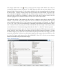
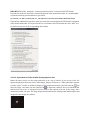
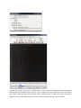
The “Multi-aperture Measurements” setup panel that was discussed previously has an option labeled
“Vary photometer aperture radii based on FWHM” and a “FWHM multiplication factor” below. The
variable aperture mode first estimates the FWHM of the object inside all of the apertures and calculates
the mean FWHM for the image. Then the aperture radii of all apertures in the image is set to FWHM x
multiplication factor. The idea is to allow the aperture radii to expand and contract with scintillation
changes and/or focus drift, etc.
IMPORTANT NOTE: The FWHM of each object is determined using only the pixels inside the defined
fixed aperture radius. It is important to set the fixed aperture radius to be larger than the largest FWHM in
the image sequence. In general, double the size of a normal case aperture radius tends to work well.
NOTE: AIJ currently overestimates FWHM. However, with the implementation in AIJ version 2.1.4,
multiplication factors in the range 1.0 to 1.4 seem to work well.
10.2.1.9. Load a Default Plot Configuration
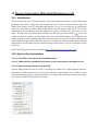
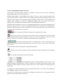
If the two “Multi-Plot” (MP) control windows are not open from the previous step, click
on the AIJ
Toolbar to open them and automatically load the measurements table just created by Multi-Aperture. Now
load the supplied plot configuration file using Multi-Plot_Main->File->”Open plot configuration from
file”. Navigate to the file “transit_standard.plotcfg” that is supplied as part of this demonstration and click
OPEN.
SHORTCUT: drag and drop the plot configuration file “transit_standard.plotcfg” onto either of the
Multi-plot control windows to open it.
10.2.1.10. Understanding the Basics of Multi-plot
10.2.1.10.1. V. Marker 1 and V. Marker 2
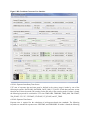
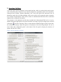
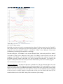
The target light curve with up to 7 comparison stars should now be displayed. However, the ingress and
egress markers may not be in the correct location for your dataset. In the top-right corner of Multi-plot
Main, you will see settings for “V. marker 1” and “V. marker 2”. Set the start of ingress time in the V.
Marker 1” box and the end of egress time in the “V. Marker 2” box. If the red dashed ingress and egress
markers are still not displayed, make sure the check boxes for each are selected.
10.2.1.10.2. Detrend and Normalize Region Selection
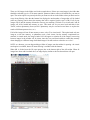
Finally, the “Detrend and Normalize Region Selection” section at the bottom of the “Multi-Plot Main”
panel needs to be set to match your data. In this simple case, click the “Copy” icon
to copy the
V.Marker1 and V.Marker2 values to the “Left” and “Right” boxes. The V.Marker lines are for display
purposes only. The “Left” and “Right” values are used to segment the data for normalization and
detrending purposes. The two sets of markers are not required to be at the same x-axis location. If the
predicted ingress and egress are not accurate, but you want to maintain those settings, simply shift the
Left and Right values to demark the desired normalization and detrending regions.
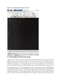
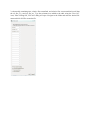
Your plot format should now look similar to the plot shown below.
SHORTCUT: control-left-click in the plot to interactively set the “Left” value, control-right-click in the
plot to set the “Right” value.