Download software error detection through testing and analysis

SOFTWARE ERROR
DETECTION THROUGH
TESTING AND ANALYSIS
J. C. Huang
University of Houston
A JOHN WILEY & SONS, INC., PUBLICATION
SOFTWARE ERROR
DETECTION THROUGH
TESTING AND ANALYSIS
SOFTWARE ERROR
DETECTION THROUGH
TESTING AND ANALYSIS
J. C. Huang
University of Houston
A JOHN WILEY & SONS, INC., PUBLICATION
C 2009 by John Wiley & Sons, Inc. All rights reserved.
Copyright Published by John Wiley & Sons, Inc., Hoboken, New Jersey.
Published simultaneously in Canada.
No part of this publication may be reproduced, stored in a retrieval system, or transmitted in any form or
by any means, electronic, mechanical, photocopying, recording, scanning or otherwise, except as
permitted under Sections 107 or 108 of the 1976 United States Copyright Act, without either the prior
written permission of the Publisher, or authorization through payment of the appropriate per-copy fee to
the Copyright Clearance Center, Inc., 222 Rosewood Drive, Danvers, MA 01923, (978) 750-8400,
fax (978) 750-4470, or on the web at www.copyright.com. Requests to the Publisher for permission
should be addressed to the Permissions Department, John Wiley & Sons, Inc., 111 River Street, Hoboken,
NJ 07030, (201) 748-6011, fax (201) 748-6008, or online at http://www.wiley.com/go/permission.
Limit of Liability/Disclaimer of Warranty: While the publisher and author have used their best efforts in
preparing this book, they make no representations or warranties with respect to the accuracy or
completeness of the contents of this book and specifically disclaim any implied warranties of
merchantability or fitness for a particular purpose. No warranty may be created or extended by sales
representatives or written sales materials. The advice and strategies contained herein may not be suitable
for your situation. You should consult with a professional where appropriate. Neither the publisher nor
author shall be liable for any loss of profit or any other commercial damages, including but not limited to
special, incidental, consequential, or other damages.
For general information on our other products and services or for technical support, please contact our
Customer Care Department within the United States at (800) 762-2974, outside the United States at
(317) 572-3993 or fax (317) 572-4002.
Wiley also publishes its books in a variety of electronic formats. Some content that appears in print may
not be available in electronic formats. For more information about Wiley products, visit our web site at
www.wiley.com.
Library of Congress Cataloging-in-Publication Data:
Huang, J. C., 1935–
Software error detection through testing and analysis / J. C. Huang.
p. cm.
Includes bibliographical references and index.
ISBN 978-0-470-40444-7 (cloth)
1. Computer software–Testing. 2. Computer software–Reliability.
computer science. I. Title.
QA76.76.T48H72 2009
005.1 4–dc22
3. Debugging in
2008045493
Printed in the United States of America
10
9
8
7
6
5
4
3
2
1
To my parents
CONTENTS
Preface
ix
1
1
Concepts, Notation, and Principles
1.1
1.2
1.3
1.4
1.5
2
3
4
Concepts, Terminology, and Notation
Two Principles of Test-Case Selection
Classification of Faults
Classification of Test-Case Selection Methods
The Cost of Program Testing
4
8
10
11
12
Code-Based Test-Case Selection Methods
14
2.1 Path Testing
2.2 Statement Testing
2.3 Branch Testing
2.4 Howden’s and McCabe’s Methods
2.5 Data-Flow Testing
2.6 Domain-Strategy Testing
2.7 Program Mutation and Fault Seeding
2.8 Discussion
Exercises
16
17
21
23
26
36
39
46
51
Specification-Based Test-Case Selection Methods
53
3.1 Subfunction Testing
3.2 Predicate Testing
3.3 Boundary-Value Analysis
3.4 Error Guessing
3.5 Discussion
Exercises
55
68
70
71
72
73
Software Testing Roundup
76
4.1
4.2
4.3
4.4
4.5
77
80
82
84
88
Ideal Test Sets
Operational Testing
Integration Testing
Testing Object-Oriented Programs
Regression Testing
vii
viii
5
6
7
CONTENTS
4.6 Criteria for Stopping a Test
4.7 Choosing a Test-Case Selection Criterion
Exercises
88
90
93
Analysis of Symbolic Traces
94
5.1 Symbolic Trace and Program Graph
5.2 The Concept of a State Constraint
5.3 Rules for Moving and Simplifying Constraints
5.4 Rules for Moving and Simplifying Statements
5.5 Discussion
5.6 Supporting Software Tool
Exercises
94
96
99
110
114
126
131
Static Analysis
132
6.1 Data-Flow Anomaly Detection
6.2 Symbolic Evaluation (Execution)
6.3 Program Slicing
6.4 Code Inspection
6.5 Proving Programs Correct
Exercises
134
137
141
146
152
161
Program Instrumentation
163
7.1 Test-Coverage Measurement
7.2 Test-Case Effectiveness Assessment
7.3 Instrumenting Programs for Assertion Checking
7.4 Instrumenting Programs for Data-Flow-Anomaly Detection
7.5 Instrumenting Programs for Trace-Subprogram Generation
Exercises
164
165
166
169
181
192
Appendix A: Logico-Mathematical Background
194
Appendix B: Glossary
213
Appendix C: Questions for Self-Assessment
220
Bibliography
237
Index
253
PREFACE
The ability to detect latent errors in a program is essential to improving program
reliability. This book provides an in-depth review and discussion of the methods of
software error detection using three different techniqus: testing, static analysis, and
program instrumentation. In the discussion of each method, I describe the basic idea
of the method, how it works, its strengths and weaknesses, and how it compares to
related methods.
I have writtent this book to serve both as a textbook for students and as a technical
handbook for practitioners leading quality assurance efforts. If used as a text, the book
is suitable for a one-semester graduate-level course on software testing and analysis
or software quality assurance, or as a supplementary text for an advanced graduate
course on software engineering. Some familiarity with the process of software quality
assurance is assumed. This book provides no recipe for testing and no discussion of
how a quality assurance process is to be set up and managed.
In the first part of the book, I discuss test-case selection, which is the crux of
problems in debug testing. Chapter 1 introduces the terms and notational conventions
used in the book and establishes two principles which together provide a unified
conceptual framework for the existing methods of test-case selection. These principles
can also be used to guide the selection of test cases when no existing method is deemed
applicable. In Chapters 2 and 3 I describe existing methods of test-case selection in
two categories: Test cases can be selected based on the information extracted form
the source code of the program as described in Chapter 2 or from the program
specifications, as described in Chapter 3. In Chapter 4 I tidy up a few loose ends and
suggest how to choose a method of test-case selection.
I then proceed to discuss the techniques of static analysis and program instrumentation in turn. Chapter 5 covers how the symbolic trace of an execution path can
be analyzed to extract additional information about a test execution. In Chapter 6 I
address static analysis, in which source code is examined systematically, manually
or automatically, to find possible symptoms of programming errors. Finally, Chapter
7 covers program instrumentation, in which software instruments (i.e., additional
program statements) are inserted into a program to extract information that may be
used to detect errors or to facilitate the testing process.
Because precision is necessary, I have made use throughout the book of concepts
and notations developed in symbolic logic and mathematics. A review is included as
Appendix A for those who may not be conversant with the subject.
I note that many of the software error detection methods discussed in this book are
not in common use. The reason for that is mainly economic. With few exceptions,
ix
x
PREFACE
these methods cannot be put into practice without proper tool support. The cost of the
tools required for complete automation is so high that it often rivals that of a major
programming language compiler. Software vendors with products on the mass market
can afford to build these tools, but there is no incentive for them to do so because
under current law, vendors are not legally liable for the errors in their products. As a
result, vendors, in effect, delegate the task of error detection to their customers, who
provide that service free of charge (although vendors may incur costs in the form of
customer dissatisfaction). Critical software systems being built for the military and
industry would benefit from the use of these methods, but the high cost of necessary
supporting tools often render them impractical, unless and until the cost of supporting
tools somehow becomes justifiable. Neverthless, I believe that knowledge about these
existing methods is useful and important to those who specialize in software quality
assurance.
I would like to take opportunity to thank anonymous reviewers for their comments;
William E. Howden for his inspiration; Raymond T. Yeh, José Muñoz, and Hal Watt
for giving me professional opportunities to gain practical experience in this field;
and John L. Bear and Marc Garbey for giving me the time needed to complete the
first draft of this book. Finally, my heartfelt thanks go to my daughter, Joyce, for
her active and affectionate interest in my writing, and to my wife, Shih-wen, for her
support and for allowing me to neglect her while getting this work done.
J. C. Huang
Houston
1
Concepts, Notation, and Principles
Given a computer program, how can we determine whether or not it will do exactly
what it is intended to do? This question is not only intellectually challenging, but
also of primary importance in practice. An ideal solution to this problem would
be to develop certain techniques that can be used to construct a formal proof (or
disproof) of the correctness of a program systematically. There has been considerable
effort to develop such techniques, and many different techniques for proving program
correctness have been reported. However, none of them has been developed to the
point where it can be used readily in practice.
There are several technical hurdles that prevent formal proof of correctness from
becoming practical; chief among them is the need for a mechanical theorem prover.
The basic approach taken in the development of these techniques is to translate the
problem of proving program correctness into that of proving a certain statement to
be a theorem (i.e., always true) in a formal system. The difficulty is that all known
automatic theorem-proving techniques require an inordinate amount of computation
to construct a proof. Furthermore, theorem proving is a computationally unsolvable
problem. Therefore, like any other program written to solve such a problem, a theorem
prover may halt if a solution is found. It may also continue to run without giving any
clue as to whether it will take one more moment to find the solution, or whether it
will take forever. The lack of a definitive upper bound of time required to complete a
job severely limits its usefulness in practice.
Until there is a major breakthrough in the field of mechanical theorem proving,
which is not foreseen by the experts any time soon, verification of program correctness
through formal proof will remain impractical. The technique is too costly to deploy,
and the size of programs to which it is applicable is too small (relative to that of
programs in common use). At present, a practical and more intuitive solution would
be to test-execute the program with a number of test cases (input data) to see if it will
do what it is intended to do.
How do we go about testing a computer program for correctness? Perhaps the
most direct and intuitive answer to this question is to perform an exhaustive test:
that is, to test-execute the program for all possible input data (for which the program
is expected to work correctly). If the program produces a correct result for every
possible input, it obviously constitutes a direct proof that the program is correct.
Unfortunately, it is in general impractical to do the exhaustive test for any nontrivial
program simply because the number of possible inputs is prohibitively large.
Software Error Detection through Testing and Analysis, By J. C. Huang
C 2009 John Wiley & Sons, Inc.
Copyright 1
2
CONCEPTS, NOTATION, AND PRINCIPLES
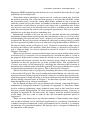
To illustrate, consider the following C++ program.
Program 1.1
main ()
{
int i, j, k, match;
cin >> i >> j >> k;
cout << i << j << k;
if (i <= 0 || j <= 0 || k <= 0
|| i+j <= k || j+k <= i || k+i <= j)
match = 4;
else if !(i == j || j == k || k == i)
match = 3;
else if (i != j || j != k || k != i)
match = 2;
else match = 1;
cout << match << endl;
}
If, for an assignment of values to the input variables i, j, and k, the output variable
match will assume a correct value upon execution of the program, we can assert that
the program is correct for this particular test case. And if we can test the program for
all possible assignments to i, j, and k, we will be able to determine its correctness.
The difficulty here is that even for a small program like this, with only three input
variables, the number of possible assignments to the values of those variables is
prohibitively large. To see why this is so, recall that an ordinary integer variable in
C++ can assume a value in the range −32,768 to +32,767 (i.e., 216 different values).
Hence, there are 216 × 216 × 216 = 248 ≈ 256 × 1012 possible assignments to the
input triple (i, j, k). Now suppose that this program can be test-executed at the rate
of one test per microsecond on average, and suppose further that we do testing 24
hours a day, 7 days a week. It will take more than eight years for us to complete an
exhaustive test for this program. Spending eight years to test a program like this is
an unacceptably high expenditure under any circumstance!
This example clearly indicates that an exhaustive test (i.e., a test using all possible
input data) is impractical. It may be technically doable for some small programs, but
it would never be economically justifiable for a real-world program. That being the
case, we will have to settle for testing a program with a manageably small subset of
its input domain.
Given a program, then, how do we construct such a subset; that is, how do we
select test cases? The answer would be different depending on why we are doing the
test. For software developers, the primary reason for doing the test is to find errors
so that they can be removed to improve the reliability of the program. In that case
we say that the tester is doing debug testing. Since the main goal of debug testing
is to find programming errors, or faults in the Institute of Electrical and Electronics
CONCEPTS, NOTATION, AND PRINCIPLES
3
Engineers (IEEE) terminology, the desired test cases would be those that have a high
probability of revealing faults.
Other than software developers, expert users of a software system may also have
the need to do testing. For a user, the main purpose is to assess the reliability so that
the responsible party can decide, among other things, whether or not to accept the
software system and pay the vendor, or whether or not there is enough confidence in
the correctness of the software system to start using it for a production run. In that
case the test cases have to be selected based on what is available to the user, which
often does not include the source code or program specification. Test-case selection
therefore has to be done based on something else.
Information available to the user for test-case selection includes the probability
distribution of inputs being used in production runs (known as the operational profile)
and the identity of inputs that may incur a high cost or result in a catastrophe if the
program fails. Because it provides an important alternative to debug testing, possible
use of an operational profile in test-case selection is explained further in Section 4.2.
We discuss debug testing in Chapters 2 and 3. Chapter 4 is devoted to other aspects
of testing that deserve our attention. Other than testing as discussed in Chapters 2
and 3, software faults can also be detected by means of analysis, as discussed in
Chapters 5 through 7.
When we test-execute a program with an input, the test result will be either correct
or incorrect. If it is incorrect, we can unequivocally conclude that there is a fault in
the program. If the result is correct, however, all that we can say with certainty is that
the program will execute correctly for that particular input, which is not especially
significant in that the program has so many possible inputs. The significance of
a correct test result can be enhanced by analyzing the execution path traversed to
determine the condition under which that path will be traversed and the exact nature
of computation performed in the process. This is discussed in Chapter 5.
We can also detect faults in a program by examining the source code systematically
as discussed in Chapter 6. The analysis methods described therein are said to be static,
in that no execution of the program is involved. Analysis can also be done dynamically,
while the program is being executed, to facilitate detection of faults that become more
obvious during execution time. In Chapter 7 we show how dynamic analysis can be
done through the use of software instruments.
For the benefit of those who are not theoretically oriented, some helpful logicomathematical background material is presented in Appendix A. Like many others
used in software engineering, many technical terms used in this book have more
than one possible interpretation. To avoid possible misunderstanding, a glossary is
included as Appendix B. For those who are serious about the material presented
in this book, you may wish to work on the self-assessment questions posed in
Appendix C.
There are many known test-case selection methods. Understanding and comparison of those methods can be facilitated significantly by presenting all methods in
a unified conceptual framework so that each method can be viewed as a particular
instantiation of a generalized method. We develop such a conceptual framework in
the remainder of the chapter.
4
CONCEPTS, NOTATION, AND PRINCIPLES
1.1
CONCEPTS, TERMINOLOGY, AND NOTATION
The input domain of a program is the set of all possible inputs for which the program
is expected to work correctly. It is constrained by the hardware on which the program
is to be executed, the operating system that controls the hardware, the programming
environment in which the program is developed, and the intent of the creator of the
program. If none of these constraints are given, the default will be assumed.
For example, consider Program 1.1. The only constraint that we can derive from
what is given is the fact that all variables in the program are of the type “short
integer” in C++. The prevailing standard is to use 16 bits to represent such data in
2’s-complement notation, resulting in the permissible range −32,768 to 32,767 in
decimal. The input domain therefore consists of all triples of 16-bit integers; that is,
D = {< x, y, z > |x, y, and z are 16-bit integers}
Input (data) are elements of the input domain, and a test case is an input used
to perform a test execution. Thus, every test case is an input, but an input is not
necessarily a test case in a particular test. The set of all test cases used in testing is
called a test set. For example, <3, 5, 2> is a possible input (or test case) in Program
1.1, and in a particular test we might choose {<1, 2, 3>, <4, 5, 6>, <0, 0, 5>, <5,
0, 1>, <3, 3, 3>} as the test set.
This notational convention for representing program inputs remains valid even
if the program accepts an input repeatedly when run in an interactive mode (i.e.,
sequence of inputs instead of a single input). All we need to do is to say that the input
domain is a product set instead of a simple set. For example, consider a program
that reads the value of input variable x, which can assume a value from set X . If
the function performed by the program is not influenced by the previous value of
x, we can simply say that X is the input domain of the program. If the function
performed by the program is dependent on the immediately preceding input, we can
make the product set X · X = {< x1 , x2 > |x1 ∈ X and x2 ∈ X } the input domain. In
general, if the function performed by the program is dependent on n immediately
preceding inputs, we can make the product set X n+1 = {< x1 , x2 , . . . , xn , xn+1 >
|xi ∈ X for all 1 ≤ i ≤ n + 1} the input domain. This is the property of a program
with memory, often resulting from implementing the program with a finite-state
machine model. The value of n is usually small and is related to the number of states
in the finite-state machine.
Do not confuse a program with memory with an interactive program (i.e., a
program that has to be executed interactively). Readers should have no difficulty
convincing themselves that an interactive program could be memoryless and that
a program with memory does not have to be executed interactively. We shall now
proceed to define some terms in program testing that might, at times, have a different
meaning for different people.
The composition of a test set is usually prescribed using a test-case selection
criterion. Given such a criterion, any subset of the input domain that satisfies the
criterion is a candidate. We say “any subset” because more than one subset in the input
CONCEPTS, TERMINOLOGY, AND NOTATION
5
domain may satisfy the same criterion. Examples of a test-case selection criterion
include T = {0, 1, 2, 3}, T = {< i, j, k > |i = j = k and k > 1 and k < 10}, and
“T is a set of inputs that cause 60% of the statements in the program to be exercised
at least once during the test.”
Let D be the input domain of a given program P, and let OK(P, d), where d ∈ D,
be a predicate that assumes the value of TRUE if an execution of program P with
input d terminates and produces a correct result, and FALSE otherwise. Predicate
OK(P, d) can be shortened to OK(d) if the omission of P would not lead to confusion.
After we test-execute the program with input d, how can we tell if OK(d) is true?
Two assumptions can be made in this regard. One is that the program specification
is available to the tester. OK(d) is true if the program produced a result that satisfies
the specification. Another is the existence of an oracle, a device that can be used to
determine if the test result is correct. The target-practice equipment used in testing
the software that controls a computerized gunsight is a good example of an oracle. A
“hit” indicates that the test is successful, and a “miss” indicates otherwise. The main
difference between a specification and an oracle is that a specification can be studied
to see how to arrive at a correct result, or the reason why the test failed. An oracle
gives no clue whatsoever.
Let T be a test set: a subset of D used to test-execute a program. A test using T is
said to be successful if the program terminates and produces a correct result for every
test case in T . A successful test is to be denoted by the predicate SUCCESSFUL(T ).
To be more precise,
SUCCESSFUL (T ) ≡ (∀t)T (OK(t))
The reader should not confuse a successful test execution with a successful program test using test set T . The test using T fails if there exists a test case in T
that causes the program to produce an incorrect result [i.e., ¬SUCCESSFUL(T ) ≡
¬(∀t)T (OK(t)) ≡ (∃t)T (¬OK(t))]. The test using T is successful if and only if the
program executes correctly for all test cases in T .
Observe that not every component in a program is involved in program execution.
For instance, if Program 1.1 is executed with input i = j = k = 0, the assignment statement match = 1 will not be involved. Therefore, if this statement is
faulty, it will not be reflected in the test result. This is one reason that a program can
be fortuitously correct, and therefore it is insufficient to test a program with just one
test case.
According to the IEEE glossary, a part of a program that causes it to produce an
incorrect result is called a fault in that program. A fault causes the program to fail
(i.e., to produce incorrect results) for certain inputs. We refer to an aggregate of such
inputs as a failure set, usually a small subset of the input domain.
In debug testing, the goal is to find faults and remove them to improve the reliability
of the program. Therefore, the test set should be constructed such that it maximizes
the probability and minimizes the cost of finding at least one fault during the test.
To be more precise, let us assume that we wish to test the program with a set of n
test cases: T = {t1 , t2 , . . . , tn }. What is the reason for using multiple test cases? It
6
CONCEPTS, NOTATION, AND PRINCIPLES
is because for all practical programs, a single test case will not cause all program
components to become involved in the test execution, and if there is a fault in a
component, it will not be reflected in the test result unless that component is involved
in the test execution.
Of course, one may argue that a single test case would suffice if the entire program
were considered as a component. How we choose to define a component for test-case
selection purposes, however, will affect our effectiveness in revealing faults. If the
granularity of component is too coarse, part of a component may not be involved in
test execution, and therefore a fault contained therein may not be reflected in the test
result even if that component is involved in the test execution. On the other hand, if
the granularity of the component is too fine, the number of test cases required and the
effort required to find them will become excessive. For all known unit-testing methods, the granularities of the component range from a statement (finest) to an execution
path (coarsest) in the source code, with one exception that we discuss in Section 7.2,
where the components to be scrutinized are operands and expressions in a statement.
For debug testing, we would like to reveal at least one fault in the test. To be more
precise, we would like to maximize the probability that at least one test case causes
the program to produce an incorrect result. Formally, we would like to maximize
p(¬OK(t1 ) ∨ ¬OK(t2 ) ∨ · · · ∨ ¬OK(tn )) = p((∃t)T (¬OK(t)))
= p(¬(∀t)T (OK(t)))
= 1 − p((∀t)T (OK(t)))
The question now is: What information can be used to construct such a test set?
It is well known that programmers tend to forget writing code to make sure that the
program does not do division by zero, does not delete an element from an empty queue,
does not traverse a linked list without checking for the end node, and so on. It may also
be known that the author of the program has a tendency to commit certain types of error
or the program is designed to perform certain functions that are particularly difficult
to implement. Such information can be used to find test cases for which the program is
particularly error-prone [i.e., the probability p(¬OK(t1 ) ∨ ¬OK(t2 ) · · · ∨ ¬OK(tn ))
is high]. The common term for making use of such information is error guessing.
The essence of that technique is described in Section 3.4.
Other than the nature or whereabouts of possible latent faults, which are unknown
in general, the most important information that we can derive from the program and
use to construct a test set is the degree of similarity to which two inputs are processed
by the program. It can be exploited to enhance the effectiveness of a test set. To see
why that is so, suppose that we choose some test case, t1 , to test the program first, and
we wish to select another test case, t2 , to test the program further. What relationship
must hold between t1 and t2 so that the joint fault discovery probability is arguably
enhanced?
Formally, what we wish to optimize is p(¬OK(t1 ) ∨ ¬OK(t2 )), the probability of
fault discovery by test-executing the program with t1 and t2 . It turns out that this probability can be expressed in terms of the conditional probability p(OK(t2 ) | OK(t1 )):
CONCEPTS, TERMINOLOGY, AND NOTATION
7
the probability that the program will execute correctly with input t2 given the fact
that the program executed correctly with t1 . To be exact,
p(¬OK(t1 ) ∨ ¬OK(t2 )) = p(¬(OK(t1 ) ∧ OK(t2 )))
= p(¬(OK(t2 ) ∧ OK(t1 )))
= 1 − p(OK(t2 ) ∧ OK(t1 ))
= 1 − p(OK(t2 ) | OK(t1 )) p(OK(t1 ))
This equation shows that if we can choose t2 to make the conditional probability
p(OK(t2 ) | OK(t1 )) smaller, we will be able to increase p(¬OK(t1 ) ∨ ¬OK(t2 )), the
probability of fault discovery.
The value of p(OK(t2 ) | OK(t1 )) depends on, among other factors, the degree
of similarity of operations performed in execution. If the sequences of operations
performed in test-executing the program using t1 and t2 are completely unrelated,
it should be intuitively clear that p(OK(t2 ) | OK(t1 )) = p(OK(t2 )), that is, the fact
that the program test-executed correctly with t1 does not influence the probability
that the program will test-execute correctly with test case t2 . Therefore, p(OK(t2 ) ∧
OK(t1 )) = p(OK(t2 )) p(OK(t1 )). On the other hand, if the sequences of operations
performed are similar, then p(OK(t2 ) | OK(t1 )) > p(OK(t2 )), that is, the probability
that the program will execute correctly will become greater given that the program
test-executes correctly with input t1 . The magnitude of the difference in these two
probabilities, denoted by
␦(t1 , t2 ) = p(OK(t2 ) | OK(t1 )) − p(OK(t2 ))
depends on, among other factors, the degree of commonality or similarity between
the two sequences of operations performed by the program in response to inputs t1
and t2 .
For convenience we shall refer to ␦(t1 , t2 ) henceforth as the (computational) coupling coefficient between test cases t1 and t2 , and simply write ␦ if the identities of
t1 and t2 are understood. The very basic problem of test-case selection can now be
stated in terms of this coefficient simply as follows. Given a test case, find another
that is as loosely coupled to the first as possible!
Obviously, the value of this coefficient is in the range 0 ≤ ␦(t1 , t2 ) ≤ 1 −
p(OK(t2 )), because if OK(t1 ) implies OK(t2 ), then p(OK(t2 ) | OK(t1 )) = 1, and if the
events OK(t1 ) and OK(t2 ) are completely independent, then p(OK(t2 ) | OK(t1 )) =
p(OK(t2 )). The greater the value of ␦(t1 , t2 ), the tighter the two inputs t1 and t2 are
coupled, and therefore the lower the joint probability of fault discovery (through the
use of test cases t1 and t2 ). Asymptotically, ␦(t1 , t2 ) becomes zero when the events of
successful tests with t1 and t2 are absolutely and completely independent, and ␦(t1 , t2 )
becomes 1 − p(OK(t2 )) = p(¬OK(t2 )) when a successful test with t1 surely entails
a successful test with t2 .
8
CONCEPTS, NOTATION, AND PRINCIPLES
Perhaps a more direct way to explain the significance of the coupling coefficient
␦(t1 , t2 ) is that
p(¬OK(t1 ) ∨ ¬OK(t2 )) = 1 − p(OK(t2 ) | OK(t1 )) p(OK(t1 ))
= 1 − ( p(OK(t2 ) | OK(t1 )) − p(OK(t2 ))
+ p(OK(t2 ))) p(OK(t1 ))
= 1 − (␦(t1 , t2 ) + p(OK(t2 ))) p(OK(t1 ))
= 1 − ␦(t1 , t2 ) p(OK(t1 )) − p(OK(t2 )) p(OK(t1 ))
The values of p(OK(t1 )) and p(OK(t2 )) are intrinsic to the program to be tested;
their values are generally unknown and beyond the control of the tester. The tester,
however, can select t1 and t2 with a reduced value of the coupling coefficient ␦(t1 , t2 ),
thereby increasing the fault-discovery probability p(¬OK(t1 ) ∨ ¬OK(t2 )).
How can we reduce the coupling coefficient ␦(t1 , t2 )? There are a number of ways
to achieve that, as discussed in this book. One obvious way is to select t1 and t2 from
different input subdomains, as explained in more detail later.
1.2
TWO PRINCIPLES OF TEST-CASE SELECTION
Now we are in a position to state two principles. The first principle of test-case
selection is that in choosing a new element for a test set being constructed, preference
should be given to those candidates that are computationally as loosely coupled as
possible to all the existing elements in the set. A fundamental problem then is: Given
a program, how do we construct a test set according to this principle? An obvious
answer to this question is to select test cases such that the program will perform a
distinctly different sequence of operations for every element in the set.
If the test cases are to be selected based on the source code, the most obvious
candidates for the new element are those that will cause a different execution path
to be traversed. Since almost all practical programs have a large number of possible
execution paths, the next question is when to stop adding test cases to the test set.
Since the purpose of using multiple test cases is to cause every component, however
that is defined, to be exercised at least once during the test, the obvious answer is to
stop when there are enough elements in the test set to cause every component to be
exercised at least once during the test.
Thus, the second principle of test-case selection is to include in the test set as
many test cases as needed to cause every contributing component to be exercised at
least once during the test. (Remark: Contributing here refers to the component that
will make some difference to the computation performed by the program. For brevity
henceforth, we omit this word whenever the term component is used in this context.)
Note that the first principle guides us as to what to choose, and the second, as to
when to stop choosing. These two principles are easy to understand and easy to apply,
TWO PRINCIPLES OF TEST-CASE SELECTION
9
and therefore become handy under situations when no existing method is applicable.
For example, when a new software system is procured, the user organization often
needs to test it to see if it is reliable enough to pay the vendor and release the system
for production runs. If an operational profile is available, the obvious choice is to
perform operational testing as described in Section 4.2. Otherwise, test-case selection
becomes a problem, especially if the system is fairly large. Source code is generally
not available to the user to make use of the methods presented in Chapter 2, and
detailed design documents or specifications are not available to use the methods
presented in Chapter 3. Even if they are available, a typical user organization simply
does not have the time, resources, and technical capability to deploy the methods. In
that event, the two principles can be utilized to select test cases. The components to be
exercised could be the constituent subsystems, which can be recognized by reading
the system user manual. Two inputs are weakly coupled computationally if they cause
different subsystems to be executed in different sequences. Expert users should be
able to apply the two principles readily to achieve a high probability of fault detection.
In short, if one finds it difficult to use any existing method, use the two principles
instead.
Next, in practical application, we would like to be able to compare the costeffectiveness of test sets. In the literature, the effectiveness of a test set is measured
by the probability of discovering at least one fault in the test (see, e.g., [FHLS98]).
It is intuitively clear that we can increase the fault-discovery capability of a test
set simply by adding elements to it. If we carry this idea to the extreme, the test
set eventually would contain all possible inputs. At that point, a successful test
constitutes a direct proof of correctness, and the probability of fault discovery is
100%. The cost of performing the test, however, will become unacceptably high.
Therefore, the number of elements in a test set must figure prominently when we
compare the cost-effectiveness of a test set. We define the cost-effectiveness of a test
set to be the probability of revealing a fault during the test, divided by the number of
elements in the test set.
A test set is said to be optimal if it is constructed in accordance with the first and
second principles for test-case selection and if its size (i.e., the number of elements
contained therein) is minimal. The concept of path testing (i.e., to choose the execution
path as the component to be exercised during the test) is of particular interest in this
connection because every feasible execution path defines a subdomain in the input
domain, and the set of all subdomains so defined constitutes a partition of the input
domain (in a set-theoretical sense; i.e., each and every element in the domain belongs
to one and only one subdomain). Therefore, a test set consisting of one element from
each such subdomain is a good one because it will not only cause every component to
be exercised at least once during the test, but its constituent elements will be loosely
coupled as well. Unfortunately, path testing is impractical in general because most
programs in the real world contain loop constructs, and a loop construct expands into
a prohibitively large number of execution paths. Nevertheless, the idea of doing path
testing remains of special interest because many known test-case selection methods
can be viewed as an approximation of path testing, as we demonstrate later.
10
1.3
CONCEPTS, NOTATION, AND PRINCIPLES
CLASSIFICATION OF FAULTS
In the preceding section we said that a test case should be selected from a subdomain
or a subset of inputs that causes a component to be exercised during the test. Is there
a better choice if there is more than one? Is there any way to improve the faultdetection probability by using more than one test case from each subdomain? The
answer depends on the types of faults the test is designed to reveal. What follows is
a fault classification scheme that we use throughout the book.
In the abstract, the intended function of a program can be viewed as a function
f of the nature f : X → Y . The definition of f is usually expressed as a set of
subfunctions f 1 , f 2 , . . . , f m , where f i : X i → Y (i.e., f i is a function f restricted to
X i for all 1 ≤ i ≤ m), X = X 1 ∪ X 2 ∪ · · · ∪ X m , and f i = f j if i = j. We shall use
f (x) to denote the value of f evaluated at x ∈ X , and suppose that each X i can be
described in the standard subset notation X i = {x | x ∈ X ∧ Ci (x)}.
Note that, above, we require the specification of f to be compact (i.e., f i = f j
if i = j). This requirement makes it easier to construct the definition of a type of
programming fault in the following. In practice, the specification of a program may
not be compact (i.e., f i may be identical to f j for some i and j). Such a specification,
however, can be made compact by merging X i and X j .
Let (P, S) denote a program written to implement the function f described above,
where P is the condition imposed on the input and S is the sequence of statements
to be executed. Furthermore, let D be the set of all possible inputs for the program.
Set D is the computer-implemented version of set X mentioned above. No other
constraints are imposed. The definition of set D, on the hand, will be constrained
by programming language used and by the hardware on which the program will be
executed. For example, if it is implemented as the short integers in C++, then D is
a set of all integers representable by using 16 bits in 2’s-complement notation. The
valid input domain (i.e., the set of all inputs for which the program is expected to
work correctly) is seen to be the set {d | d ∈ D and P(d)}. The program should be
composed of n paths:
(P, S) = (P1 , S1 ) + (P2 , S2 ) + · · · + (Pn , Sn )
Here (Pi , Si ) is a subprogram designed to compute some subfunction f j . P ≡ P1 ∨
P2 ∨ · · · ∨ Pn , and P is in general equal to T (true) unless the programmer places
additional restrictions on the inputs. We shall use S(x) to denote the computation
performed by an execution of S with x as the input.
Two basic types of fault may be committed in constructing the program (P, S).
The program created to satisfy a specification must partition its input domain into at
least as many subdomains as that required by the specification, each of which must be
contained completely in some subdomain prescribed by the specification. Otherwise,
there is a domain fault. If there is an element in the input domain for which the
program produces a result different from that prescribed by the specification, and the
input is in a subdomain that is contained completely in a subdomain prescribed by
CLASSIFICATION OF TEST-CASE SELECTION METHODS
11
the specification, there is a computational fault. To be more precise, we can restate
the definitions as follow.
1. Computational fault. The program has a computational fault if (∃i)(∃ j)((Pi ⊃
C j ∧ Si (x) = f j (x)).
2. Domain fault. The program has a domain fault if ¬(∀i)(∃ j)(Pi ⊃ C j ).
In words, if the program specification says that the input domain should consist
of m subdomains X 1 , X 2 , . . . , X m , the program should partition the input domain
into n subdomains D1 , D2 , . . . , Dn , where n must be greater than or equal to m
if the partition prescribed by the specification is compact. The partition created by
the program must satisfy the condition that every Di = {d | d ∈ D and Pi (d)} be
contained completely in some X j , X 1 ∪ X 2 ∪ . . . ∪ X m = X , and D1 ∪ D2 ∪ . . . ∪
Dn = D. Otherwise, there is a domain fault.
If there is a subdomain Di created by the program that is contained completely in
some X j prescribed by the specification, then for every input in Di , the value computed by Si must be equal to that computed by f j . Otherwise, there is a computation
fault.
It is possible that a program contains both domain and computational faults at the
same time. Nevertheless, the same element in the input domain cannot be involved in
both kinds of fault. If the program is faulty at a particular input, it is either of domain
or computational type, but not both.
Previously published methods of program-fault classification include that of
Goodenough and Gerhart [GOGE77], Howden [HOWD76], and White and Cohen
[WHCO80]. All three include one more type of fault, called a subcase fault or
missing-path fault, which occurs when the programmer fails to create a subdomain
required by the specification [i.e., if ¬(∀i)(∃ j)(Ci ⊂ P j )]. Since such a fault also
manifests as a computational fault, we chose, for simplicity, not to identify it as a
fault of separate type.
In Chapters 2 and 3 we discuss test-case selection methods that are designed
particularly for revealing the domain faults. In such methods, the components to be
exercised are the boundaries of subdomains embodied by the predicates found in the
source code or program specification.
1.4
CLASSIFICATION OF TEST-CASE SELECTION METHODS
It was observed previously that when a program is being test-executed, not all constituent components would be involved. If a faulty component is not involved, the fault
will not be reflected in the test result. A necessary condition, therefore, for revealing
all faults in a test is to construct the test set in such a way that every contributing
component in the program is involved (exercised) in at least one test execution!
What is a component in the statement above? It can be defined in many different ways. For example, it can be a statement in the source code, a branch in the
12
CONCEPTS, NOTATION, AND PRINCIPLES
control-flow diagram, or a predicate in the program specification. The use of different components leads to the development of different test-case selection methods. As
shown in Chapters 2 and 3, many test-case selection methods have been developed.
If the component used is to be identified from the source code, the resulting testcase selection method is said to be code-based. The most familiar examples of such
a method are the statement test, in which the program is to be tested to the extent that
every statement in its source code is exercised at least during the test, and the branch
test, in which the program is to be tested to the extent that every branch in its controlflow diagram is traversed at least once during the test. There are several others that
cannot be explained as simply. All the methods are discussed in detail in Chapter 2.
If the component used is to be identified from the program specification, the
resulting test-case selection method is said to be specification-based. Examples of the
components identifiable from a program specification include predicates, boundaries
of input/output variables, and subfunctions. Chapter 3 is devoted to a discussion of
such methods.
It is possible that certain components can be identified from either the source
code or the program specification. The component defined in the subfunction testing
method discussed in Chapter 3 is an example.
Since a component can be also a subdomain consisting of those and only those
inputs that cause that component to be exercised during the test, a test-case selection
method that implicitly or explicitly requires execution of certain components in
the program during the test can also be characterized as being subdomain-based
[FHLS98]. The test methods and all of their derivatives, discussed in Chapters 2 and
3, are therefore all subdomain-based.
Are there any test-case selection methods that are not subdomain-based? There are
at least two: random testing [DUNT84, CHYU94, BOSC03] and operational testing
[MUSA93, FHLS98]. The first, although interesting, is not discussed in this book
because its value has yet to be widely recognized. The second is important in that it
is frequently used in practice. Because it is neither code- nor specification-based, we
choose to discuss it in Section 4.2.
1.5
THE COST OF PROGRAM TESTING
Software testing involves the following tasks: (1) test-case selection; (2) test execution; (3) test-result analysis; and if it is debug testing, (4) fault removal and regression
testing.
For test-case selection, the tester first has to study a program to identify all input
variables (parameters) involved. Then, depending on the test-case selection method
used, the tester has to analyze the source code or program specification to identify all
the components to be exercised during the test. The result is often stated as a condition
or predicate, called the test-case selection criterion, such that any set of inputs that
satisfies the criterion is an acceptable test set. The tester then constructs the test cases
by finding a set of assignments to the input variables (parameters) that satisfies the testcase selection criterion. This component of the cost is determined by the complexity
of the analysis required and the number of test cases needed to satisfy the criterion.
THE COST OF PROGRAM TESTING
13
A commonly used test-case selection criterion is the statement test: testing the program to the extent that every statement in the source code is exercised at least once
during the test. The critics say that this selection criterion is far too simplistic and ineffectual, yet it is still commonly used in practice, partly because the analysis required
for test-case selection is relatively simple and can be automated to a great extent.
The process of test-case selection is tedious, time consuming, and error prone. The
most obvious way to reduce its cost is through automation. Unfortunately, some parts
of that process are difficult to automate. If it is specification based, it requires analysis
of text written in a natural language. If test cases satisfying a selection criterion are to
be found automatically, it requires computational power close to that of a mechanical
theorem prover.
For operational testing, which we discuss in Section 4.2, the cost of test-case
selection is minimal if the operational profile (i.e., the probability distribution of
inputs to be used in production runs) is known. Even if the operational profile had to
be constructed from scratch, the skill needed to do so is much less than that for debug
testing. That is one of the reasons that many practitioners prefer operational testing.
It should be pointed out, however, that a real operational profile may change in time,
and the effort required to validate or to update an existing profile is nontrivial.
Test execution is perhaps the part of the testing process that is most amenable to
automation. In addition to the machine time and labor required to run the test, the
cost of test execution includes that of writing the test harness (i.e., the additional
nondeliverable code needed to produce an executable image of the program).
The cost of test-result analysis depends largely on the availability of an oracle. If
the correctness of test results has to be deduced from the specification, it may become
tedious, time consuming, and error prone. It may also become difficult to describe
the correctness of a test result if it consists of a large aggregate of data points, such
as a graph of a photographic image. For that reason, the correctness of a program is
not always unequivocally definable.
A class of computer programs called real-time programs have hard time constraints; that is, they not only have to produce results of correct values but have to
produce them within prescribed time limits. It often requires an elaborate test harness
to feed the test cases at the right time and to determine if correct results are produced
in time. For that reason, a thorough test of a real-time software system is usually
done under the control of an environment simulator. As the timing aspect of program
execution is not addressed in this work, testing of real-time programs is beyond the
scope of this book.
Finally, it should be pointed out that, in practice, the ultimate value of a test method
is not determined solely by the number of faults it is able to reveal or the probability
that it will reveal at least one fault in its application. This is so because the possible
economical consequence of a fault could range from nil to catastrophic, and the value
of a program often starts to diminish beyond a certain point in time. A test method is
therefore of little value in practice if the faults it is capable of revealing are mostly
inconsequential, or if the amount of time it takes to complete the test is excessive.
2
Code-Based Test-Case
Selection Methods
We start by discussing a family of test methods that can be used to do debug testing,
and the test cases are to be selected based on the information that can be extracted from
the source code. In debug testing, as explained in Chapter 1, we want to maximize
the probability that at least one fault will be revealed by the test. That is, if we use
a test set of n elements, say, T = {t1 , t2 , . . ., tn }, we want to maximize the probability
p(¬OK(t1 ) ∨ ¬OK(t2 ) ∨ · · · ∨ ¬OK(tn )) = p((∃t)T (¬OK(t)))
= p(¬(∀t)T (OK(t)))
= 1 − p((∀t)T (OK(t)))
How do we go about constructing such a test set? We can do it incrementally by
letting T = {t1 } first. If there is any information available to find a test case that has
a high probability of revealing a fault in the program, make it t1 . Otherwise, t1 can be
chosen arbitrarily from the input domain.
We then proceed to add another test case t2 to T so that the probability of fault
discovery is maximal. That probability can be expressed as
p(¬OK(t1 ) ∨ ¬OK(t2 )) = p(¬(OK(t1 ) ∧ OK(t2 )))
= p(¬(OK(t2 ) ∧ OK(t1 )))
= 1 − p(OK(t2 ) ∧ OK(t1 ))
= 1 − p(OK(t2 ) | OK(t1 )) p(OK(t1 ))
As explained in Chapter 1, this can be achieved by finding another test case, t2 ,
such that t1 and t2 are as loosely coupled as possible; that is, ␦(t1 , t2 ), the coupling
coefficient between t1 and t2 , is minimal. The value of ␦(t1 , t2 ) is a function of the
degree of exclusiveness between the sequences of operations to be performed by the
program in response to test cases t1 and t2 .
Software Error Detection through Testing and Analysis, By J. C. Huang
C 2009 John Wiley & Sons, Inc.
Copyright 14
CODE-BASED TEST-CASE SELECTION METHODS
15
Now if we proceed to find t3 , the third element for the test set, the fault discovery
probability to maximize is
p(¬OK(t1 ) ∨ ¬OK(t2 ) ∨ ¬OK(t3 ))
= p(¬(OK(t1 ) ∧ OK(t2 ) ∧ OK(t3 )))
= p(¬(OK(t3 ) ∧ OK(t2 ) ∧ OK(t1 )))
= 1 − p(OK(t3 ) ∧ OK(t2 ) ∧ OK(t1 ))
= 1 − p(OK(t3 ) | OK(t2 ) ∧ OK(t1 )) p(OK(t2 ) ∧ OK(t1 ))
Again, this probability can be maximized by minimizing the conditional probability
p(OK(t3 ) | OK(t2 ) ∧ OK(t1 )), that is, the probability that the program will execute
correctly with t3 given that the program executed correctly with t1 and t2 . Obviously,
this can be accomplished by selecting t3 such that neither OK(t1 ) nor OK(t2 ) will
have much, if any, impact on the probability p(OK(t3 )). That is, t3 should be chosen
such that both ␦(t1 , t3 ) and ␦(t2 , t3 ) are minimal.
This process can be repeated to add inputs to the test set. In general, to add a new
element to the test set T = {t1 , t2 , . . . , ti }, the (i + 1)th test case ti+1 is to be selected
to maximize the probability
p(¬OK(t1 ) ∨ · · · ∨ ¬OK(ti ) ∨ ¬OK(ti+1 ))
= p(¬(OK(t1 ) ∧ · · · ∧ OK(ti ) ∧ OK(ti+1 )))
= p(¬(OK(ti+1 ) ∧ OK(ti ) ∧ · · · ∧ OK(t1 )))
= 1 − p(OK(ti+1 ) ∧ OK(ti ) ∧ · · · ∧ OK(t1 ))
= 1 − p(OK(ti+1 ) | OK(ti ) ∧ · · · ∧ OK(t1 )) p(OK(ti ) ∧ · · · ∧ OK(t1 ))
This probability can be maximized by minimizing the conditional probability
p(OK(ti+1 ) | OK(ti ) ∧ · · · ∧ OK(t1 )), that is, by selecting ti+1 in such a way that
␦(t1 , ti+1 ), ␦(t2 , ti+1 ), . . . , ␦(ti , ti+1 ) are all minimal. In practice, there are several different ways to do this, each of which led to the development of a different test-case
selection method, discussed in this and the following chapters.
In studying those methods, keep in mind that program testing is a very practical
problem. As such, the value of a debug test method is predicated not only on its
capability to reveal faults but also by the cost involved in using it. There are three
components to the cost: the cost of finding test cases, the cost of performing test
execution, and the cost of analyzing the test results. The number of test cases used
has a direct impact on all three components. Therefore, we always strive to use as few
test cases as possible. The amount of training and mental effort required to construct a
test set is a major factor in determining the cost of test-set construction. Therefore, in
developing a test method, whenever alternatives are available to accomplish a certain
task, we invariably choose the one that is most cost-effective. In some studies, the
cost of debug testing includes the cost of removing the faults detected as well. This
16
CODE-BASED TEST-CASE SELECTION METHODS
is rightly so, because the main purpose of debug testing is to improve the reliability
of a software system by detecting and removing latent faults in the system.
To facilitate understanding of the test-case selection methods discussed below, it
is useful to think that every method for debug testing is developed as follows. First, a
type of programming construct, such as a statement or branch predicate, is identified
as the essential component of a program each component of which must be exercised
during the test to reveal potential faults. Second, a test-case selection criterion is
established to guide the construction of a test set. Third, an analysis method is devised
to identify such constructs in a program and to select test cases from the input domain
so that the resulting test set is reasonable in size and its elements are loosely coupled
computationally. Those are the essential elements of every debug test method.
2.1
PATH TESTING
In path testing, the component to be exercised is the execution path. The test-case
selection criterion is defined to select test cases such that every feasible execution path
in the program will be traversed at least once during the test. Path testing is interesting
in that every feasible execution path defines a subdomain in the input domain, and the
resulting set of subdomains constitutes a partition of the input domain. That is, the
intersection of any two subdomains is an empty set, and the union of all subdomains is
the input domain. In other words, every input belongs to one and only one subdomain,
and the subdomains are not overlapping.
If two test cases are selected from the same subdomain, they will be tightly coupled
computationally because they will cause the program to test-execute along the same
execution path and thus perform the same sequence of operations. On the other hand,
if two test cases are selected from different subdomains of this sort, they will cause the
program to test-execute along two different execution paths and thus perform different
sequences of operations. Therefore, they will have a smaller coupling coefficient, as
explained previously. Any subset of the input domain that contains one and only one
element from each subdomain defined by the execution paths in the program will
satisfy the test-case selection criterion, and the test cases will be loosely coupled.
Path testing is not practical, however, because almost all real-world programs
contain loop constructs, and each loop construct often expands into a very large
number of feasible execution paths. Besides, it is costly to identify all subdomains,
find an input from each, and determine the corresponding correct output the program
is supposed to produce. Despite its impracticality, we choose to discuss path testing
first because all test-case selection methods discussed in the remainder of the chapter
can be viewed as an approximation of path testing. Originally, these methods were
developed independently based on a variety of ideas as to what is important in a
program. The two test-case selection principles developed in Section 1.2 provide a
unified conceptual framework based on which of these methods can be described as
different instantiations of a generalized method—path testing. Instead of exercising
all execution paths, which is impractical in general, only a sample of them will be
exercised in these methods. Basically, these methods differ in the ways in which
the paths are sampled. These methods are made more practical by reducing the