1
LAGOPUS – Divergence time estimation in R
using the multidivtime approach
Christoph Heibl and Natalie Cusimano
Manual for the current version 1.4.4 as released on April 12, 2010
Contents
1 Introduction
2 Required software
2.1 Getting R and the ape package .
2.2 Getting LAGOPUS . . . . . . . . .
2.3 Getting phyloch (optional) . . .
2.4 Getting PAML and multidivtime
2
.
.
.
.
.
.
.
.
.
.
.
.
.
.
.
.
.
.
.
.
.
.
.
.
.
.
.
.
.
.
.
.
.
.
.
.
.
.
.
.
.
.
.
.
.
.
.
.
.
.
.
.
.
.
.
.
.
.
.
.
.
.
.
.
.
.
.
.
.
.
.
.
.
.
.
.
.
.
.
.
.
.
.
.
.
.
.
.
.
.
.
.
.
.
.
.
2
2
3
3
3
3 Preparing the data
3.1 DNA sequence alignments . . . . .
3.2 Phylogenetic trees . . . . . . . . .
3.3 Age constraints . . . . . . . . . . .
3.4 Creating the LAGOPUS input object
.
.
.
.
.
.
.
.
.
.
.
.
.
.
.
.
.
.
.
.
.
.
.
.
.
.
.
.
.
.
.
.
.
.
.
.
.
.
.
.
.
.
.
.
.
.
.
.
.
.
.
.
.
.
.
.
.
.
.
.
.
.
.
.
.
.
.
.
.
.
.
.
.
.
.
.
.
.
.
.
.
.
.
.
.
.
.
.
.
.
.
.
3
4
4
4
5
4 Running LAGOPUS
4.1 Checking and editing the control files . . . . . . . . . . . . . . . . . . . . . .
4.2 Fixing the path to the executables . . . . . . . . . . . . . . . . . . . . . . .
4.3 Starting the analysis . . . . . . . . . . . . . . . . . . . . . . . . . . . . . . .
6
6
6
6
5 Acknowledgements
7
1
1
Introduction
Bayesian relaxed-clock dating with PAML 4.1 (Yang, 2007) and multidivtime (Thorne
et al., 1998; Kishino et al., 2001; Thorne and Kishino, 2002) is currently one of the most
widely used molecular dating techniques. However, the procedure can be tedious and
error-prone because many different steps are involved. “The software is unintentionally
user-rude”, as put by Jeff Thorne in the multidivtime user manual. In order to facilitate
using PAML/multidivtime for R users (and others that might be convinced here ...) we
wrote a small R add-on package that offers easy access to Bayesian relaxed-clock dating
once the input data are specified. The package is called LAGOPUS in order to distinguish it
in this manual from multidivtime. LAGOPUS offers you:
• Input and control files are written automatically to the corresponding directories
(and without typos, of course).
• Running baseml, paml2modelinf, estbranches, multidivtime in a pipe.
• Age constraints are automatically assigned to the corresponding nodes. Correct assignment of nodes can be verified in a cladogram that is printed to the screen with
the age constraints mapped on it.
• The ‘amount of evolution’ needed for calculating the mean and the standard deviation of the prior distribution for the rate at the root node (rtrate and rtratesd,
respectively), is estimated by the median of branch lengths (see the multidivtime
read-me).
• The output is summarized in an object of class mdt and can be visualized conveniently
by the function plot.mdt.
If this is what you are looking for, read on ...
2
2.1
Required software
Getting R and the ape package
Source code and binaries for the latest releases of R for all major platforms are distributed
on http://cran.r-project.org/. We recommend to install the binary distribution. Once
installed you can launch the R console by doubleclicking on the R application in your
applications folder (or wherever you chose to install it) or by typing open -a R in your
shell. The ape package can be installed by the install.packages command. Make sure
to install also the dependencies:
install.packages(‘‘ape’’, dependencies = TRUE).
For further information type ?install.packages in the R console. Upon successful installation, ape is loaded by library(ape).
2
2.2
Getting LAGOPUS
Download the gzipped LAGOPUS package from the LAGOPUS website (http://www.christophheibl.
de/mdt/mdtinr.html). It is not necessary to unpack the file, just open a shell, change to
the directory where the gzipped file has been stored, and type:
R CMD INSTALL LAGOPUS 1.4.2.tar.gz
Alternatively, you can install LAGOPUS via the R console:
install.packages(‘‘LAGOPUS 1.4.2.tar.gz’’, repos = NULL, type = ‘‘source’’)
2.3
Getting phyloch (optional)
The phyloch package contains easy-to-use functions to import DNA sequences. Other
packages (e.g., ape, seqinr) contain quite the same functionality and perhaps you prefere
those. If you decide to use phyloch, download it from http://www.christophheibl.de/
Rpackages.html and install it exactly like the LAGOPUS package.
2.4
Getting PAML and multidivtime
To carry out the Bayesian dating analysis, baseml from Ziheng Yang’s PAML package
and paml2modelinf, estbranches, and multidivtime from the multidivtime package by
Jeffrey Thorne and Hirohisa Kishino are required.
PAML is distributed on the website of Ziheng Yang (http://abacus.gene.ucl.ac.uk/
software/paml.html) and multidivtime can be down loaded from Jeffrey Thorne’s website
(http://statgen.ncsu.edu/thorne/multidivtime.html). For compilation and installation of these programs please refer to the information provided in the respective manuals
and read-me’s. A helpful step-for-step manual for PAML/multidivtime was written by
Frank Rutschmann and can be downloaded at ftp://statgen.ncsu.edu/pub/thorne/
bayesiandating1.5.pdf.
IMPORTANT: In order to use LAGOPUS all the executables must be stored in one single
folder. The easiest way to achieve this is to copy the baseml executable into the multidistribute folder. On our computer this looks like this:
cp /Applications/paml4/src/baseml /Applications/multidistribute
3
Preparing the data
This section tells you how to prepare your data. In order to start your analysis you
need one or more alignments of DNA sequences, one or more phylogentic trees (with or
without branch lengths) and a table containing the age constraints to use on the data. The
following paragraphs show how to do this. You can skip them if you know how to deal with
3
phylogenetic data in R. We suggest that you create a folder (e.g., R_files/multidivtime)
where you drop your sequence and tree files.
3.1
DNA sequence alignments
First, read in your alignment file(s). If you installed and loaded the phyloch package (see
above), this can be done easily calling
my.sequences <- read.align("my.sequences").
read.align can parse files in NEXUS, PHILIP, and FASTA format. Alternatively you
can read in sequence data in the same formats by the functions provided by the ape
package. Type ?read.dna and ?read.nexus.data for details. In ape DNA sequence
alignments are stored as an object of mode matrix and class DNAbin. Before proceeding
you should check if the input file has been correctly parsed. This can be done, e.g., by
typing summary(my sequences). If the issued base frequencies seem reasonable, usually
everything is alright.
3.2
Phylogenetic trees
Now you proceed reading in your phylogenetic tree(s). You can use either
my.tree <- read.tree("my.tree.tre") or
my.tree <- read.nexus("my.tree.nex"),
both provided by the ape package. The first command is for trees saved in the NEWICK
format, the latter for the NEXUS format. The input tree can contain branch lenghts which
are dropped automatically by LAGOPUS.
3.3
Age constraints
The age constraints are stored in a data frame object. The example tree in figure 1 will
demostrate the procedure. Suppose you want to constrain nodes A and B to have been
present at least 72 my and 12 my before present. To identify both nodes you have to
specify for each of them two terminal nodes that coalesce in these nodes. The fossil record
normally provides a minimal age for the node in question (because we cannot be sure if
there aren’t any unknown, older fossils out there), and this characteristic is represented by
‘L’ which stands for lower bound. If you are completely sure that the node cannot be older
(e.g., strains of viruses, etc.), you might also specify ‘U’ for upper bound, which means a
maximal age. To sum up all this information we type:
node.A <- c("L", "t9", "t3", 72)
node.B <- c("L", "t5", "t4", 12)
my.age.constraints <- data.frame(rbind(node.A, node.B))
4
t12
t11
t10
t9
t8
t7
A
●
t6
B
●
t4
t5
t3
t2
t1
Figure 1: An example tree with two internal nodes A and B which are represented in the
fossil record 72 and 12 mya, respectively.
Again you can check the data frame by typing my.age.constraints. Note that age constraints, which involve the outgroup taxa are not allowed in multidivtime. This is because the outgroup will be pruned from the input tree in the MCMC analysis. In this case
LAGOPUS will issue a warning and terminate.
3.4
Creating the LAGOPUS input object
If you have created all these necessary objects (i.e., sequence alignment, phylogenetic tree,
and age constraints) you will have to bundle them into an input object. This is achieved
by the mdt.in function. For an unpartitioned dataset this looks like:
x <- mdt.in(my.sequences, my.tree, my.age.constraints)
The function checks the consistency of the input objects and stores them in a list of class
mdt.in.
If you want to analyze a partitioned data set, you will have to also specify a ‘final tree’.
This is necessary because the first step of parameter estimation using baseml requires
5
that each tree match its corresponding alignment partition perfectly. Subsequent steps
(estbranches and multidivtime) relax this requirement, so that you can select one tree
for the final estimation of node ages and substitution rates. mdt.in recognizes the first
tree in its argument list as ‘final tree’.
x <- mdt.in(seq1, seq2, seq3, final.tr, tr1, tr2, tr3, age.constraints)
x <- mdt.in(seq1, seq2, seq3, tr1, tr2, tr3, age.constraints)
# in the latter example tr1 is recognized as final tree
4
4.1
Running LAGOPUS
Checking and editing the control files
Load the baseml and the multidivtime control files and edit them if necessary. For example
you should specify a mean (rttm) and standard deviation (rttmsd) for the prior distribution
of the root node age, i.e. the time interval from the root to present. The choice of this
value depends on the prior knowledge about the studied organisms.
data(baseml.ctr)
data(multicntrl.dat)
multicntrl.dat$rttm <- 84
multicntrl.dat$rttmsd <- 84
4.2
# set rttm to 84 mya
# set rttmsd to 84 mya
Fixing the path to the executables
The multidivtime function has one argument path whose default is NULL. In order to save
typing every time you start an analysis, you can store the path in a *.RData object and
load it prior to execution of multidivtime. On CH’s system this looks like this:
path <- "/Applications/multidistribute"
save("path", file = "path.RData")
# before execution of multidivtime
load("/Users/R files/multidivtime/path.RDat")
4.3
Starting the analysis
Once you have created your input object, you are ready to execute multidivtime. The
interface is as follows:
multidivtime(x, file = NULL, start = "baseml", part = 1, runs = 1,
path = NULL, transfer.files = TRUE, LogLCheck = 100, plot = TRUE)
6
Below follows a list with explanations of the arguments:
x
file
start
part
runs
path
transfer.files
LogLCheck
5
An object of class mdt.in containing DNA sequence alignment,
phylogeny, and constraints (see 3).
A character string giving a name to the output files, e.g, file =
"mdt.august2008". If left NULL, the output files will be called
"LAGOUT".
The step to start with. Can either be baseml, estbranches, or
multidivtime. If a step later than baseml is chosen, the file
argument must not be changed in order to allow LAGOPUS the
accession of the previous output files.
If several partitions are to be analyzed, LAGOPUS can be started or
restarted on any partition. The number of the partition is specified
as an integer. E.g., part = 2 skips the first partition.
It is recommended to run Bayesian analyses several times to
check for the convergence of the posterior probability distributions.
LAGOPUS offers a simple way to do this via the runs argument. An
integer gives the number of MCMC chains to run, e.g., runs = 3.
A character string giving the path to the executables of baseml,
paml2modinf, estbranches, and multidivtime, which must all
reside in the same directory (see 2.4). It is convenient to store
the path in a file and load it prior to executation of LAGOPUS as
described in 4.2.
Logical. If transfer.files = TRUE, all output files are transferred to an output folder, which is created in the working directory of R. If transfer.files = FALSE, the output files will stay
in the directory where the executables are.
A real number giving the maximal difference between log Likelihood values of baseml and estbranches that will be accepted
by LAGOPUS. If the value of LogLCheck is exceeded, the program
assumes that one of the Likelihood estimations failed and will terminate. This mechanism is somewhat arbitrary and you should
not blindly rely on it.
Acknowledgements
Jeff Thorne provided the algorithm for node assignment for phylogentic trees used by
multidivtime, Emmanuel Paradis reported several issues with multidivtime and gave
advice for improvement, Hanno Schäfer offered his data set on Ctenoplectra bees for testing, and Susanne Renner gave useful comments on running multidivtime and tested the
manual.
7
References
Kishino, H., J. L. Thorne, and W. J. Bruno. 2001. Performance of a divergence time
estimation method under a probabilistic model of rate evolution. Mol. Biol. Evol. 18:352–
361.
Thorne, J. L. and H. Kishino. 2002. Divergence time and evolutionary rate estimation with
multilocus data. Syst. Biol. 51:689–702.
Thorne, J. L., H. Kishino, and I. S. Painter. 1998. Estimating the rate of evolution of the
rate of molecular evolution. Mol. Biol. Evol. 15:1647–1657.
Yang, Z. 2007. Paml 4: a program package for phylogenetic analysis by maximum likelihood. Mol. Biol. Evol. 24:1586–1591.
8