Download Microphone lab

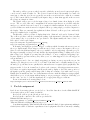
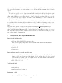
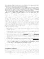
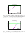
BME 194: Applied Circuits Lab 2: Electret Microphones
Kevin Karplus
January 12, 2013
1
Design Goal
For this lab, you will
• characterize the DC behavior of an electret microphone, using the Arduino to automate the
measurement,
• design a simple circuit to bias the microphone appropriately to have an output that is centered
at 1v,
• observe the waveform of the microphone on the oscilloscope, and
• design a very simple high-pass (DC-blocking) filter to convert the microphone output from
being centered at 2.5v to being centered at 0v, using just resistors and capacitors.
Much of this lab is familiarization with the oscilloscope (DC and AC coupling, input scaling,
X1/X10 probes, time base, triggering, . . . ) and with the Arduino data logger.
2
Background
Electret microphone
An electret microphone consists of a permanently charged capacitor (an “electret”) connected to
the gate of a field-effect transistor. One plate of the capacitor is a diaphragm, moved by the changes
in air pressure that make up sound.
Because the charge on the electret is constant, but the capacitance changes with the separation
between plates of the capacitor, the voltage across the capacitor changes with the separation:
V (t) = Q/C(t) .
The small change in voltage is converted to a change in the saturation current of the field-effect
transistor (FET), which can be measured externally. We will look at field-effect transistors more
carefully in a later lab: for this lab we are mainly interested in looking at the electret microphone
as a simple sensor, but some of the FET behavior will appear in the DC characterization of the
microphone.
Read http://en.wikipedia.org/wiki/Electret
and http://en.wikipedia.org/wiki/Electret microphone
Oscilloscope
An oscilloscope is a device for visualizing a time-varying voltage. There are two main types: analog
and digital.
http://en.wikipedia.org/wiki/Oscilloscope
1
The analog oscilloscopes use a cathode-ray tube, which shoots an electron beam at a phosphorcoated screen to make a bright dot. The electron beam is deflected horizontally by a sawtooth
waveform, so that the spot moves repeatedly across the screen from left to right at a constant
speed. The beam is deflected vertically by the input voltage, so that what appears on the screen is
the voltage as a function of time.
The digital oscilloscopes record the input voltage for a chunk of time, then display it on the
screen. The recorded data can be manipulated in various ways that are not feasible with the
analog scope, and the data can be saved on a computer for further analysis. It is now possible to
get devices that serve as the front-end of a digital oscilloscope, using a laptop or tablet computer for
the display. These are currently less sophisticated than dedicated oscilloscopes, but considerably
cheaper for similar levels of capability.
Traditionally, oscilloscopes have a display that is 10 “divisions” wide and 8 “divisions” high.
The oscilloscopes have controls for setting the scaling of the inputs and of the time base, in terms
of how many volts or seconds there are per division. The inputs usually also have a choice of
DC-coupled or AC-coupled input.
http://en.wikipedia.org/wiki/Capacitive coupling
http://en.wikipedia.org/wiki/Direct coupling
Both analog and digital scopes have “trigger” conditions, which determine when a sweep across
the scope display starts. These trigger conditions can be based on any of the inputs to the scope
(there is often an additional input to the scope available only for triggering). On analog scopes,
the trigger is usually a voltage level and whether the input signal is rising or falling as it crosses
that voltage level. Digital scopes may have the ability to do more complicated triggering logic.
Because digital scopes have memory, they allow you to see what happened before the trigger, as
well as afterward.
The triggers can be done once (single triggering), producing one sweep across the screen. On
digital scopes, this gives you a record of a one-time event that can be carefully analyzed, but on
an analog scope, the fluorescence quickly fades, unless the trace is captured photographically. The
triggers can also be done in “normal” mode, where each occurrence of the trigger starts a new trace.
If you have a repetitive input signal, this allows the analog display to show the same portion of
the signal repeatedly, giving a stable image (like looking at a rotating object with a stroboscope).
Finally, there is usually an “auto” mode that starts a new trace without waiting for a trigger signal,
which allows you to see the input without having to set proper trigger conditions. Generally, you
use the “auto” mode to look at the signal and choose appropriate trigger conditions.
For more information about triggering look at
http://hobbyprojects.com/oscilloscope tutorial/oscilloscope trigger controls.html
3
Pre-lab assignment
Read about electret microphones, as cited above. Read the data sheet for the CMA-4544PF-W
electret microphone we’ll be using for this lab.
Read about oscilloscopes in general, as cited above.
Read about the controls for the oscilloscopes in the lab:
Kikusui COS5041 analog scope
http://www.kikusui.co.jp/kiku manuals/C/COS5040 5041 E.PDF
Tektronix TDS3052 2-channel digital storage scope.
Somewhat surprisingly, Tektronix hides their user manual behind a login requirement, making it
relatively inaccessible to students or purchasers of used equipment. Given how extremely confusing
2
their control panels are without a manual, this is extremely short-sighted of them—if students have
bad experiences learning to use their equipment, who will specify the equipment later? I found a
copy at
http://www.cs.washington.edu/education/courses/cse466/07wi/labs/l2/Oscope/TDS3000Manual.pdf
The analog scopes are easier to learn to use and will be sufficient for this lab, though the digital
scopes offer considerably more capability if you can figure out the controls. Despite the inventory
claims on the BELS web pages, there appear to be more digital scopes than analog scopes in the
lab, so you’ll probably have to learn to use them at least minimally—you can’t be sure that the
simpler analog scopes will be available.
Read how to use the function generators in the lab: Agilent 33120A. You won’t need most of
the capability of those function generators (which are really overkill for a beginning circuits course),
just how to generate a sine wave of known frequency, which is covered in pages 19–21 of the User’s
Guide:
http://www.home.agilent.com/upload/cmc upload/All/6C0633120A USERSGUIDE ENGLISH.pdf
Prepare gnuplot scripts for plotting current versus voltage and equivalent resistance versus
voltage, including fitting different models. You’ll probably have to tweak these scripts once you get
real data, but you’ll want to have a usable basis to start from, rather than spending all your lab
time reading gnuplot documentation.
4
Parts, tools, and equipment needed
Parts for this lab from kit:
• CUI inc CMA-4544PF-W electret microphone
http://www.digikey.com/product-detail/en/CMA-4544PF-W/102-1721-ND/1869981
• resistors
• 10kΩ trimpot
• breadboard
• loudspeaker
Parts students need to provide on their own:
• Arduino board. Drivers should be installed on lab computers for Uno, Uno R3, Duemilanove, and Leonardo versions of the Arduino board. Arduino Mega boards not tested
yet, but should work on your own computer if the drivers are installed. Arduino Due
not supported by the Data Logger.
• USB cable for board.
Tools for this lab:
• wire cutters
• wire strippers
• small screwdriver for trimpot
Equipment in lab:
• power supply (for providing power to microphone)
3
Figure 1: Back of the electret microphone. In this orientation, the lower terminal is “Terminal 2”,
which should be connected to ground, and the upper terminal is “Terminal 1”, which should be
connected via a series resistor to the positive voltage source (or terminal 2 to the positive power
rail, and terminal 1 via a series resistor to ground).
• multimeter (for measuring current and voltage)
• oscilloscope (for observing signal)
• function generator (for producing a sound signal for mic)
5
Procedures
DC characterization with multimeter
The first part of the lab is to measure the DC current through the microphone for various DC
voltages across it. With the equipment in the lab, this is most easily done by hooking up a
multimeter configured as an ammeter in series with the mic, and powering the pair from the
bench power supply. Connecting clip leads to the mic can be difficult, but the mic plugs into the
breadboard easily, allowing wires or double-ended header pins to be used as probe points. Be sure
to get the polarity right, as shown in Figure 1.
Measure the current at several different voltages (say 1–10 volts in steps of 1 volt). Note that
the data sheet specifies a maximum voltage for the microphone. Don’t exceed it.
Record the voltages and currents in a table and try to fit the I-vs-V curve with various functions.
If your measurements are all for voltages over 1v, you should see fairly constant current.
DC characterization with Arduino
Measuring with the multimeter and recording the data by hand in a lab notebook or by typing it
into a file is tedious, and so relatively few data points well be taken. This makes it easy to miss
important phenomena, so let’s automate the measurement. The goal is to use the Data Logger
from C:\ProgramFiles\DataLogger\ or
http://bitbucket.org/abe k/arduino-data-logger/get/default.tar.bz2
to record numbers from which you can derive either an I-vs-V curve or an R-vs-V curve (where the
resistance here is the DC resistance R = V /I not the dynamic resistance dV
dI ).
There are some limitations of the Arduino analog-to-digital converter that are important for
this lab:
4
ñÿðï
ùþ
ùòñý
ÿø
þýüûú
÷öõ
ôöóþ ôöóø
ÿþ
þýüûú
ùòñþ
îíì
Figure 2: Schematic for testing the the DC characteristics of the microphone. The voltage source
is the bench power supply. Schematic drawn using http://www.circuitlab.com/editor/
• There are only 6 channels that can be recorded on (for Uno and other ATmega328-based
boards—some of the newer boards have more pins that can be used as analog inputs).
• The highest voltage allowed is 5v and the lowest is 0v.
• The resolution is only 10 bits (1024 steps).
• The steps seem to be more uniformly spaced at the low end of the range than the high end
(so differences at the high end are less accurate than differences at the low end).
• The external reference voltage AREF must be at least 0.5v (this is not in the data sheet, but
when I tried lower AREF voltages, the reading was always 1023), and no more than 5v.
• Readings are not simultaneous, but the analog-to-digital converter is quickly switched from
one input to another. It takes at least 104µs for each conversion. For slowly changing signals,
this skewing of the inputs in time doesn’t matter much, but for fast-changing signals it can
make a big difference.
• The Arduino has limited memory size for queuing recordings and will drop data points if its
queue is full. The serial line rate of 115200 baud means that you can’t sample inputs more
frequently than once per millisecond with one analog channel, adding about 0.5msec for each
additional analog channel. (The Leonardo, using a different USB protocol may be able to get
a little more speed out of the USB channel, to the point where the Python program on the
host computer becomes a more important bottleneck.)
The Arduino can only record voltages (as well as digital values and timestamps), so we need to
convert the current through the microphone into a voltage that we can measure with the Arduino.
The circuit in Figure 2 provides one way to do this. The bench power supply provides a known
voltage that is used as the AREF reference voltage of the Arduino’s analog-to-digital converter, the
18-turn trimmer potentiometer (trimpot) allows us to present a lower voltage to the microphone
plus 10kΩ resistor that act as a voltage divider. We can use two analog inputs of the Arduino
to record the voltage across the resistor (which we can convert to a current through the resistor,
5
since we know the resistance) and the voltage across both the microphone and the resistor. If we
subtract VA1 from VA0 we get the voltage across the microphone.
Since you are connecting an external voltage reference to AREF, be sure to specify the “external”
option in the data logger configuration pane. Your files will be much easier to work with if you
have the data logger compute the voltages of A0 and A1 for you. Also, remember to document in
the notes what A0 and A1 are connected to, so that you can interpret the files later.
For two or three different settings of AREF (say 0.55v, 1.7v, and 5v), record a series of measurements (say every 100ms) as you adjust the trimpot from one end of its range to the other.
Each different AREF setting will need a different output file for the data, since the DataLogger
puts metadata in the file about the settings used.
[Note: you can do this part of the lab at home without the bench power supply, by using the 5v
supply from the Arduino board, but you need to measure what voltage that is with a multimeter—
it depends on the power being delivered through the USB port, which can fluctuate quite a bit
and still be within the USB spec. The bench supply is a much more reliable DC signal. Getting
lower AREF voltages than 5v at the input to the trimpot using just the Arduino may require using
another trimpot as a voltage divider to divide down the 5V supply. ]
Write a gnuplot script to plot the data as I-vs-V points and as R-vs-V points. I found it useful
to plot each file separately (so the points are color-coded by which file they cam from), but to make
a larger file by concatenating all the separate files for fitting models to the data. Plotting with log
scales on both axes makes the data look simpler and easier to come up with models for. Using a
linear scale for voltage may hide the low-voltage behavior.
Here are four models to try fitting:
• linear (resistance) model: I = V /RL . You may want to fit RL for just the lower voltages
across the microphone.
• saturation (current source) model: I = Isat . You may want to fit the saturation current Isat
for just the higher voltages across the microphone.
q
q
2 + (V /I
2
2
2
• blended linear and saturation model: R(V ) = RL
sat ) or I(V ) = V / RL + (V /Isat ) .
This makes a smooth transition from the linear model to the saturation model, with the
limV →0 R(V ) = RL and limV →∞ R(V ) = Isat /V . This model is similar to a standard model
for FET behavior.
• power-law model. The saturation current, as I measured it, was not constant,
q but increased
2 + (V p /I
2
slightly as voltage increased. I modeled this with a power law: R(V ) = RL
sat )
q
2 + (V p /I
2
or I(V ) = V / RL
sat ) . If p = 1, this is the same as the previous model, but with
p < 1, the current goes up with voltage even in the saturation region.
The current-versus-voltage plots for the four models are shown in Figures 3 and 4.
When I tried this lab, I got a very good fit with the last model, except at very low voltages and
currents, where the quantization errors of the Arduino made measurement unreliable.
Microphone to oscilloscope
You will be converting the current output of the electret microphone to a voltage output by putting
the mic in series with a load resistor connected to a +5 v power supply (like a voltage divider, but
with the microphone between the output and ground). Using your measurements or the formula
you found for the I-vs-V curve, compute what resistance this load resistor should have to get a 1v
6
Current vs. voltage for electret mic
Current through mic [microA]
100
10
1
linear model
saturation current
blended model
power law in saturation region
0.1
0.001
0.01
0.1
Voltage across mic [V]
1
10
Figure 3: Current-versus-voltage plot for the electret mic. The log scale for current makes the lowvoltage behavior clearer. For this figure, I’ve deliberately suppressed the data and the parameters I
got, to give the flavor of the models. Your plots should, of course, include the data and you should
use “sprintf” in the titles of the plotted curves to print the parameters of the models.
Current vs. voltage for electret mic
250
Current through mic [microA]
200
150
100
50
linear model
saturation current
blended model
power law in saturation region
0
0.001
0.01
0.1
Voltage across mic [V]
1
10
Figure 4: Current-versus-voltage plot for the electret mic. The linear scale for current makes the
high-voltage behavior clearer. Again, I’ve suppressed the data and the parameters.
7
ñðï
ÿþýüûú
ïþüìö
ïþëî
îí
ùýø÷öõøöôóò÷
Figure 5: Schematic for the microphone, the load resistor, and the DC-blocking capacitor. You
will need to fill in the values used. I’ve used a standard nFET symbol for the electret microphone
(rather than square box I used in Figure 2), because CircuitLab does not have a symbol for a
microphone. Schematic drawn using http://www.circuitlab.com/editor/
output voltage. Choose the closest standard resistance value from your collection of resistors, and
measure the DC voltage you actually get.
Now hook up the oscilloscope probe to the output of the microphone and try to view the output
of the microphone as a time-varying signal. You can whistle or talk into the mic or provide some
other sound source. It may be easiest to learn to use the scope if you have a known input signal.
One way to get that is to hook up the function generator to a loudspeaker to put out a sine wave
of known frequency, say between 50Hz and 5kHz. Try using both AC coupling and DC coupling
for the scope input, and see what happens if you change the triggering conditions.
What is the amplitude of the AC output of the microphone? The AC amplitude is half the
peak-to-peak voltage—that is, it is the maximum voltage minus the minimum voltage, divided by
2. Note that this amplitude will depend on how loud your sound input is.
Add a DC-blocking capacitor to the microphone as shown in Figure 5 and connect scope probes
to both Vout and VAC . Use the oscilloscope to compare the output of the microphone at the two
points at different frequencies of input. Use the multimeter(s) to measure the RMS AC voltage at
the two points for different frequencies (say 5Hz, 10Hz, 20Hz, 50Hz, 100Hz, . . . , 50kHz). Plot the
ratio RM S(VAC )/RM S(Vout ) as a function of frequency. don’t move your speaker or microphone
around during these tests, as you don’t want to change the relationship between the two. Your
hands and body can act as important reflectors of sound also, so keep them well away from the mic
and speaker during this test.
Note: the effect should be different depending on what size capacitor you use, particularly at
the lower frequencies. Try a few different sizes, from 470µF down to 100pF.
6
Demo and writeup
Demo the oscilloscope outputs to a TA or instructor, showing that you know how to adjust the
time base, the input scaling, and the triggering.
On the Monday after the lab, turn in a writeup describing what you did. Remember that the
instructors are not your audience—a bioengineer who has not read the assignment is.
Provide at least
8
• a purpose of the report (the problem you are solving or the design information you are
providing),
• the I-vs-V or R-vs-V curves for the electret microphone (which electret microphone?),
• a schematic of the tested circuit,
• a plot of the ratio of the RMS voltage after the DC-blocking capacitor to the RMS voltage
before the DC-blocking capacitor as a function of frequency.
7
Design Hints
When trying to come up with a function for the I-vs-V curve, look at the plot with different ways
of scaling the x and y coordinates.
To choose a suitable initial DC-blocking capacitor value for testing, try to block frequencies
below about 50 Hz (much higher than one would normally want to use). Use the pull-up resistor
1
you chose as the resistance and the RC time constant RC = 2πf
for a cutoff frequency f to compute
the capacitance. If that works, try a capacitor about 50 times larger, to get a 1Hz cutoff.
We’ll look at RC filtering in more detail later in the quarter.
9