1
GE Healthcare
Optima MR360
1.5T MR system
Operator Manual
GE Medical Systems does business as GE Healthcare
Volume I / Volume II
Optima MR360
1.5T MR System
Operator Manual, English
5339461-1EN Rev 4 (10/2010)
Copyright 2010 General Electric Company
All rights reserved.
Medical Device Directive
Medical Device Directive
These products conform with the requirements of council directive 93/42/EEC concerning medical
devices, when they bear the following CE Mark of Conformity:
Manufacturer:
GE HANGWEI MEDICAL SYSTEMS CO., LTD
No. 2, North Yong Chang Street
Economic-Technological Development Zone
Beijing, P.R. CHINA 100176
European Representative:
GE Medical Systems S.C.S
Quality Assurance Manager
283 rue de la Minière
78530 BUC France
Telephone: +33 1 30 70 40 40
This equipment generates, uses, and can radiate radio frequency energy. The equipment may cause
radio frequency interference with other medical and non-medical devices and radio communications.
To provide reasonable protection against such interference, the:
GE MR Systems
comply with emissions limits for (Group 2, Class A) Medical Devices as stated in EN 60601-1-2. However, there is no guarantee that interference will not occur in a particular installation.
If this equipment is found to cause interference (which may be determined by turning the equipment
on and off), the user (or qualified service personnel) should attempt to correct the problem by one or
more of the following measures:
o
o
o
o
reorient or relocate the affected devices;
increase the separation between the equipment and the affected device;
power the equipment from a source different from that of the affected device; and/or
consult the point of purchase or service representative for further suggestions.
The manufacturer is not responsible for any interference caused by using interconnect cables that are
not recommended or by unauthorized changes or modifications to this equipment. Unauthorized
changes or modifications could void the user’s authority to operate the equipment.
5339461-1EN Rev 4
Copyright 2010 General Electric Company
CE-1
Medical Device Directive
Do not use devices that transmit RF Signals (cellular phones, transceivers, or radio controlled products) in the vicinity of this equipment as they may cause performance outside the published specifications. Keep the power to these types of devices turned off when near this equipment.
The medical staff in charge of this equipment is required to instruct technicians, patients, and other
people who may be around this equipment to fully comply with the above requirement.
Immunity/Emissions Exceptions: Note the exceptions from the EMC test results. Check with the business EMC engineer for this information.
In accordance with the international safety standard IEC 60601-1, this system is a Class I device,
acceptable for Continuous Operation, having ordinary protection against ingress of water (IPX0) with
type B and BF applied parts and is not for use in the presence of flammable anesthetics.
CAUTION: This symbol indicates that the waste of electrical and electronic equipment must
not be disposed as unsorted municipal waste and must be collected separately. Contact an authorized representative of the manufacturer for information concerning the decommissioning of your
equipment.
NOTE: This system uses Ryobi fonts for Japanese screen display.
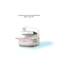
Indications for use
The Optima MR360 is a whole body magnetic resonance scanner designed to support high resolution,
high signal-to-noise ratio, and short scan times. It is indicated for use as a diagnostic imaging device
to produce axial, sagittal, coronal, and oblique images, spectroscopic images, parametric maps,
and/or spectra, dynamic images of the structures and/or functions of the entire body, including, but
not limited to, head, neck, TMJ, spine, breast, heart, abdomen, pelvis, joints, prostate, blood vessels,
and musculoskeletal regions of the body. Depending on the region of interest being imaged, contrast
agents may be used.
The images produced by the Optima MR360 reflect the spatial distribution or molecular environment
of nuclei exhibiting magnetic resonance. These images and/or spectra when interpreted by a trained
physician yield information that may assist in diagnosis.
CE-2
5339461-1EN Rev 4 (10/2010)
Copyright 2010 General Electric Company
Table of Content
Table of Content
Chapter 1: Read Me First
1-1
MR workflow
1-1
MR Operator Information
1-3
How to Use Your Online Help
1-4
Online Help Procedures
1-5
Chapter 2: About this manual
About this manual
Chapter 3: Get Acquainted Training
System User Interface
Chapter 4: Applications
2-1
2-1
3-1
3-1
4-1
Applications annotation
4-1
Multi Station
4-2
Real Time
4-8
SmartPrep
4-28
Procedures
4-33
Chapter 5: Cardiac
5-1
Patient setup
5-1
Plane procedure
5-11
Workflows
5-23
Procedures
5-28
Chapter 6: Equipment
Equipment Procedures
6-1
6-1
Chapter 7: Film
7-1
Film methods
7-1
Film preferences
7-7
Procedures
Chapter 8: Filters
7-11
8-1
Filters Procedures
8-1
Chapter 9: FuncTool
9-1
FuncTool Procedures
9-1
Film Save
9-43
Generate Report
9-48
Right-click functions
9-53
Chapter 10: HIPAA
10-1
General
10-1
Group
10-4
User
10-7
Procedures
10-11
Screens
10-12
5339461-1EN Rev 4 (10/2010)
Copyright 2010 General Electric Company
TOC-1
Table of Content
Chapter 11: Imaging Options
11-1
Imaging Options annotation
11-1
Procedures
11-3
SmartPrep
11-29
Real Time
11-34
Multi-Station
11-54
Multi-Phase
11-60
IDEAL
11-65
ASSET
11-70
Chapter 12: Image Management
12-1
Image Management Procedures
12-1
Recycle Bin
12-3
Patient List
12-6
Chapter 13: Image Management Archive Network
Image Management Archive Network Procedures
Chapter 14: Image Management Data Apps
13-1
13-1
14-1
CD/DVD
14-1
Data Export
14-7
Procedures
14-13
Chapter 15: Image Management Session Apps
Image Management Session Apps Procedures
Chapter 16: Image Management Tools
Image Management Tools Procedures
Chapter 17: Patient Preparation
15-1
15-1
16-1
16-1
17-1
Patient padding
17-1
Procedures
17-5
Chapter 18: Preferences
Preferences Procedures
Chapter 19: Prescan
Prescan Procedures
Spectroscopy
Chapter 20: Protocol Notes
Protocols Note Procedures
Chapter 21: Protocols
Protocols Procedures
18-1
18-1
19-1
19-1
19-13
20-1
20-1
21-1
21-1
Protocol Exchange
21-15
Protocol Lockout
21-24
Protocol Notes
21-25
Chapter 22: PSD
PSD Procedures
TOC-2
22-1
22-1
5339461-1EN Rev 4 (10/2010)
Copyright 2010 General Electric Company
Table of Content
3-Plane localizer
22-4
EPI
22-5
FSE
22-13
GRE
22-24
PROPELLER
22-52
Spectroscopy
22-57
Spin Echo
22-80
Vascular
22-84
Chapter 23: Respiratory
Respiratory Procedures
Chapter 24: Scan
Scan Procedures
23-1
23-1
24-1
24-1
Artifact tips
24-28
AutoStart
24-42
AutoVoice
24-46
Graphic Rx
24-55
SAT
24-87
Artifact control
24-92
Contrast
24-96
Resolution
24-111
Timing
24-117
Standard parameters
24-136
Stop Watch
24-147
Workflow Manager
24-149
Chapter 25: Sessions
25-1
Desktop Navigation
25-1
Procedures
25-2
Chapter 26: System Management
System Management Procedures
Chapter 27: System Startup and Shutdown
26-1
26-1
27-1
Daily Automated Quality Assurance
27-1
Procedures
27-8
Chapter 28: User CV
User CV Procedures
Chapter 29: Viewer
Viewer Procedures
28-1
28-1
29-1
29-1
Annotation
29-23
Cross Reference
29-25
Film
29-31
Matte
29-35
5339461-1EN Rev 4 (10/2010)
Copyright 2010 General Electric Company
TOC-3
Table of Content
Measure
29-38
Text Page
29-47
User Preferences
29-49
Window Width and Level
29-60
Chapter 30: Viewer CD
30-1
Viewer CD Procedures
30-1
Chapter 31: Viewer GSPS
31-1
Viewer GSPS Procedures
Chapter 32: Viewer InLine
Viewer InLine Procedures
31-1
32-1
32-1
Annotation
32-31
Cross Reference
32-39
Film
32-45
Matte
32-50
Measure
32-54
Propagate
32-58
ROI
32-64
Window Width and Level
32-68
Chapter 33: Viewer Mini
Viewer Mini Procedure
Chapter 34: Viewer SR
33-1
33-1
34-1
Viewer SR Procedures
34-1
Chapter 35: Volume Viewer
35-1
Annotation
Batch Film
35-1
35-5
Color and Shading
35-13
Histogram
35-16
IVI
35-18
Measure
35-23
Model
35-31
ROI
35-33
Segment
35-38
Procedures
35-45
Chapter 36: Worklist Manager
Worklist Manager Procedures
TOC-4
36-1
36-1
5339461-1EN Rev 4 (10/2010)
Copyright 2010 General Electric Company
Chapter 1: Read Me First
Chapter 1: Read Me First
MR workflow
The MR system's role in the workflow for an exam is to acquire data and create images for analysis of
the patient's condition. The operator needs to be able to start with the patient's requested procedure,
execute the set of acquisitions and post-processing activities to fulfill that request and then transfer/export the resulting data.
MR exam workflow
5339461-1EN Rev 4 (10/2010)
Copyright 2010 General Electric Company
1-1
Chapter 1: Read Me First
MR exam workflow
No.
1.
Description
Patient handling (1)
The patient is brought into the MR scan room and prepared for the exam.
1. Transfer the Patient Procedure
2. Position the Patient Procedure
3. Landmark the Patient Procedure
2.
To start scanning upon closing the magnet room door, Scan with Auto Start. The
magnet room door must be closed to start scanning to avoid bidirectional transmission of RF energy outside the room, which can degrade image quality.
Patient Registration (2a and 2b)
The patient is entered into the Worklist Manager through either a RIS system or manually
entered and a protocol is attached to the patient's exam.
Enter a Patient in Work List Procedure
The scan data is acquired (2c)
A protocol must be attached to the exam before you can start exam.
3.
Scan with a Protocol Procedure
View and analyze images (3)
After the scan data is acquired the images can be viewed and filmed (3a) and analyzed
(3b) using one of several post processing applications
Open InLine Viewer procedure
Open Viewer procedure
Open the film composer procedure
Open Volume Viewer procedure
Open FuncTool procedure
Add/Subtract procedure
Pasting procedure
4.
Store images (4)
The exam can be networked to be analyzed on an AW workstation (4a), stored and
analyzed on a PACs system (4b) or simply stored on a CD/DVD (4c)
Auto Archive Procedure
Auto Network procedure
Manual send Archive Network Procedure
Save Images to CD/DVD Procedure
1-2
5339461-1EN Rev 4 (10/2010)
Copyright 2010 General Electric Company
Chapter 1: Read Me First
MR Operator Information
Your MR operator information is comprised of the following sources:
l
l
l
l
OnLine Help - an electronic document that resides on your MR system. It is opened by clicking
the online help icon
.
Release Notes (optional) - delivered in paper or CD/DVD.
MR Safety Guide - delivered in paper.
Depending on the country in which your MR system was purchased, your operator documentation may include regulatory information, which may be delivered in paper or on a
CD/DVD.
5339461-1EN Rev 4 (10/2010)
Copyright 2010 General Electric Company
1-3
Chapter 1: Read Me First
How to Use Your Online Help
Your MR operator manual is on line. The online help icon
screen.
is located in the footer area of the
The online help initially appears in the lower right corner of the screen when the online help icon is
clicked. The online help window overlays the waveform and Protocol Notes area. The online help window can be closed or minimized. If you minimize the window, then the next time you click the online
help icon, the window opens at the same size and in the same location on the screen.
The online help is an html document which means that much of the content is hyper-linked. Click blue
text to link to another topic or to view drop down text or images. If you have linked to another topic,
use the back and forward arrow keys
between topics.
on the Mozilla browser to navigate
Procedures
Open procedure
Open TOC procedure
View movies procedure
Online Help window resize procedure
Print topics procedure
Minimize procedure
Close procedure
1-4
5339461-1EN Rev 4 (10/2010)
Copyright 2010 General Electric Company
Chapter 1: Read Me First
Online Help Procedures
Online Help open procedure
In the footer area of the screen, click the Online Help icon
.
Related topics
Online Help introduction
5339461-1EN Rev 4 (10/2010)
Copyright 2010 General Electric Company
1-5
Chapter 1: Read Me First
Online Help open the TOC procedure
The default state for the table of contents is open. If the Index or Search view is open, click Contents
to open the table of contents.
Click a book and all the topics related to the book title are displayed.
1-6
5339461-1EN Rev 4 (10/2010)
Copyright 2010 General Electric Company
Chapter 1: Read Me First
Related topics
Online Help introduction
5339461-1EN Rev 4 (10/2010)
Copyright 2010 General Electric Company
1-7
Chapter 1: Read Me First
Online Help window resize procedure
Click and drag any edge of the Online Help window.
Related topics
Online Help introduction
1-8
5339461-1EN Rev 4 (10/2010)
Copyright 2010 General Electric Company
Chapter 1: Read Me First
Online Help minimize procedure
Click the dot in the upper right corner of the help window. The next time you open help, the window
opens at the same size and in the same location on the screen.
Related topics
Online Help introduction
5339461-1EN Rev 4 (10/2010)
Copyright 2010 General Electric Company
1-9
Chapter 1: Read Me First
Online Help view system screens and images
Move the cursor around the image or graphic. If the cursor changes from a pointer to a hand, click to
link to another topic that has text related the graphic.
Related topics
Online Help introduction
1-10
5339461-1EN Rev 4 (10/2010)
Copyright 2010 General Electric Company
Chapter 1: Read Me First
Online Help view movies
If there is a movie in a topic, it automatically plays as soon as the topic is opened. To view the movie a
second time, click the back and forward buttons on the Mozilla browser. This closes and opens the
topic and thus restarts the movie.
Related topics
Online Help introduction
5339461-1EN Rev 4 (10/2010)
Copyright 2010 General Electric Company
1-11
Chapter 1: Read Me First
Online Help print topics procedure
Use this procedure to print topics from the PC version of Online Help.
1. Click all light purple text to open the drop-down text, if printing all the text within a topic is
desired.
2.
In the Online Help, click
on the toolbar.
3. In the Print Topics dialog, select either Print the selected topic or Print the selected heading
and all subtopics.
l
If you choose the latter option, all pages in the selected table of contents book will be printed.
4. Click Print.
5. In the Print menu, select the printer and number of copies.
Related topics
Online Help introduction
1-12
5339461-1EN Rev 4 (10/2010)
Copyright 2010 General Electric Company
Chapter 1: Read Me First
Online Help close procedure
Click the close icon and select Close from the pull-down menu. The next time you open help, it will
open to the title page and the default size and location.
Related topics
Online Help introduction
5339461-1EN Rev 4 (10/2010)
Copyright 2010 General Electric Company
1-13
Chapter 1: Read Me First
[This page intentionally left blank]
1-14
5339461-1EN Rev 4 (10/2010)
Copyright 2010 General Electric Company
Chapter 2: About this manual
Chapter 2: About this manual
About this manual
This section explains the purpose and design of this Online Help. It is an introduction to the manual,
providing information on the purpose, prerequisite skills, organization, format, and graphic conventions that identify the visual symbols used throughout the manual.
This manual is for Optima MR360 MR Systems . The manual does not identify components or features
that are standard or purchasable options. Therefore, if a feature or component included in the manual
is not on your system, it is either not available on your system configuration or your site has not purchased the option.
Safety information
Please refer to the MR Safety Guide, direction # 2381696. The MR Safety Guide describes the safety
information you and the physicians must understand thoroughly before you begin to use the system. If
you need additional training, seek assistance from qualified GE Healthcare personnel.
The equipment is intended for use by qualified personnel only.
This manual should be kept with the equipment and should be readily available at all times. It is important for you to periodically review the procedures and safety precautions. It is important to read and
understand the contents of this manual before attempting to use this product.
Federal Law restricts this device to sale, distribution, and use by or on the order of a physician.
Purpose of this manual
This manual is written for health care professionals (namely, the MR technologist) to provide the necessary information relating to the proper operation of this system. The manual is intended to teach
you the system components and features necessary to use your MR system to its maximum potential.
It is not intended to teach magnetic resonance imaging or to make any type of clinical diagnosis.
Prerequisite skills
This manual is not intended to teach the principles of magnetic resonance imaging. It is necessary for
you to have sufficient knowledge to competently perform the various diagnostic imaging procedures
within your modality. This knowledge is gained through a variety of educational methods, including
clinical working experience, hospital-based programs, or classes offered by many college and university Radiologic Technology diagnostic imaging programs.
Pop-up windows
Pop-up message windows require an acknowledgement typically by clicking OK. Always click OK to
acknowledge the message.
If there are multiple floating window on the screen, click on the window title to bring it in front or close
the window in front to access the windows that is behind it.
Mouse controls
The mouse is a hand-operated device that you maneuver across the surface of a pad. As you move it,
the on-screen cursor mimics the movement of the mouse, allowing you to move among windows and
menus. For instance, moving the mouse to the right causes the on-screen cursor to move to the right.
The mouse is used to make selections by clicking the left, right, and middle buttons.
Mouse: 1 = Left button, 2 = Middle button, 3 = Right button
5339461-1EN Rev 4 (10/2010)
Copyright 2010 General Electric Company
2-1
Chapter 2: About this manual
Mouse action
Click
Right-click
Middle-click
Click and drag
Right-click and drag
Middle-click and drag
Double-click
Triple-click
Description
Clicking the left mouse button to select a button or icon.
Clicking the right mouse button.
Clicking the middle mouse button.
Clicking and holding the left mouse button down while dragging
the cursor to the desired location.
Clicking and holding the right mouse button down while dragging the cursor to the desired location.
Clicking and holding the middle mouse button down while dragging the cursor to the desired location.
Clicking the left mouse button twice in rapid succession.
Clicking the left mouse button three times in rapid succession.
Graphic conventions and legends
This manual uses special conventions for images and legends to make it easier for you to work with
the information. The table below describes the conventions used when working with menus, buttons,
text boxes, and keyboard keys.
Example
Select
Press Enter
Press and hold Shift
Click Viewer
In the Spacing text box ...
Type supine in the Patient
Position text box
Select Sort > Sort by date
Ctrl X simultaneously
2-2
Description
Selecting an option in a check box or radial button and selecting a tab.
Pressing a hard key on the keyboard.
Pressing and holding down a hard key on the keyboard.
A button label or Interface button name.
The name of text box in which you can select or type text.
Text you enter into a text box.
The pathway of selecting option(s) in a pull-down menu.
Press and hold the Control button on the keyboard and simultaneously press the X button on the keyboard. Ctrl is the abbreviation used for the Control keyboard button, and ALT is the
abbreviation used for the Alternative keyboard.
5339461-1EN Rev 4 (10/2010)
Copyright 2010 General Electric Company
Chapter 2: About this manual
Safety notices
The following safety notices are used to emphasize certain safety instructions. This manual uses the
international symbol along with the danger, warning, or caution message. This section also describes
the purpose of an Important notice and a Note.
DANGER
Danger is used to identify conditions or actions for which a specific hazard is known to exist that will
cause severe personal injury, death, or substantial property damage if the instructions are ignored.
WARNING
Warning is used to identify conditions or actions for which a specific hazard is known to exist that may
cause severe personal injury, death, or substantial property damage if the instructions are ignored.
CAUTION
Caution is used to identify conditions or actions for which a potential hazard may exist that will or can
cause minor personal injury or property damage if the instructions are ignored.
COIL CAUTION
Coil Caution is used to identify conditions or actions for which a potential hazard of crossing or looping
coil cables may exist that will or can cause minor personal injury or property damage if the instructions are ignored.
Important indicates information where adherence to procedures is crucial or where your comprehension is necessary to apply a concept or effectively use the product.
Note provides additional information that is helpful to you. It may emphasize certain information
regarding special tools or techniques, items to check before proceeding, or factors to consider about
a concept or task.
Troubleshooting tips provide information that allow you to investigate the resolution of some
type of problem, locate the difficulty, and make adjustments to solve the problem.
5339461-1EN Rev 4 (10/2010)
Copyright 2010 General Electric Company
2-3
Chapter 2: About this manual
[This page intentionally left blank]
2-4
5339461-1EN Rev 4 (10/2010)
Copyright 2010 General Electric Company
Chapter 3: Get Acquainted Training
Chapter 3: Get Acquainted Training
System User Interface
Footer area of screen layout
The message and icons in the footer area always appear on the screen.
Footer area
Description
Message area that displays messages regarding the system status. Click the arrow next to the message to display the error log screen.
The Scan Parameter area also has a Scan messages
area that is related to the series in an INRX state
Click Hardware icon to display controls for:
gating
magnet light and fan
The current Date and Time is displayed. It is set by your
service engineer.
The Reconstruction Status area displays the status of the
examination, series, and images currently being reconstructed. The most recently reconstructed image is displayed until the next image is ready for reconstruction.
The Network Status area displays the status of the examination, series, and images currently being networked
and the destination location.
The Archive/Remove Status area displays the status of
the examination, series, and images currently being
archived to the primary archive device. The Remove
Status simply shows "Removing" or "Removed." The
individual exams, series or images are not listed.
The Film Status area displays the status of the examination, series, and images currently being filmed.
5339461-1EN Rev 4 (10/2010)
Copyright 2010 General Electric Company
3-1
Chapter 3: Get Acquainted Training
Roll the cursor over the icon to display the disk capacity
for 256 and 512 images.
The graph displays multiple disk capacity states:
empty
¼ full
½ full
¾ full
a red segment when there is insufficient space available for the currently prescribed acquisition.
Click to open an iLinq window.
Click to open the Stop Watch screen.
Click to open the on line help window.
Click SAR1 icon to open the SAR display.
1Specific Absorption Rate
3-2
5339461-1EN Rev 4 (10/2010)
Copyright 2010 General Electric Company
Chapter 3: Get Acquainted Training
Header area
The icons and session tabs in the header area always appear on the screen.
Header area
Work area
Click Scan Session tab to view the:
Scan work area screen
InLine Viewer work area displays when InLine
Viewer is active in the scan session
Three scan sessions are allowed (one active
and two Scan Done)
Click Protocol Session tab to view the Protocol
work area.
One protocol session is allowed.
Click Review Session tab to view Review work
area.
Up to two review sessions are allowed if system
resources are available.
Click Worklist Manager icon to display the Worklist Manager work area. The Worklist Manager
area is used to:
Schedule patients
Select patients for scan activities
Enter patient demographic information
Complete HIS/RIS tasks
Start an exam
Click Image Management icon to display the
Image Management work area. The Image Management work area is used to:
Archive/network images
Select an exam/series/image
Launch an application from the Session Management, Data Management or Tools lists
5339461-1EN Rev 4 (10/2010)
Copyright 2010 General Electric Company
3-3
Chapter 3: Get Acquainted Training
Click Tools icon to display the Tools work area.
The Tools work area has multiple tabs that open
unique work areas that are used to:
Open a protocol session to create or edit protocols from the Protocol Organize tab
Initiate a TPS Reset from the Service Desktop
Manager tab
Define multiple system settings from the
Guided Install feature on the Service Desktop
Manager tab
Define several system preferences from the
System Preferences selection on the Tools
pull-down menu
View error log and write a note to your service representative on the GESYS tab
View and select options on the Gating Control
screen from the GATING tab
The menu allows access to additional functions
3-4
5339461-1EN Rev 4 (10/2010)
Copyright 2010 General Electric Company
Chapter 3: Get Acquainted Training
Terminology
Control panels
Control panels are comprised of selectable buttons. Feature applications such as FuncTool, Volume
Viewer, InLine Viewer, and Viewer all have control panels.
Linking
Linking allows you to connect series or images in scan and volume viewer.
Pull-down menus
A drop-down or pull-down menu capability is indicated by an arrow. For example, all session tabs
have drop-down menus.
Screen
Screens or windows are free floating. They typically appear within a workflow and require you to
respond before you can move to the next step in the workflow. An example of a screen is the SAR and
dB/dt screen that appears in the New Patient workflow.
Session
A session is a workflow activity involving scan, review, and/or protocols. Sessions are identified by
tabs displayed in the header or across the top of the screen. The tab always indicates the session
type.
Tabs
Tabs are used through-out the user interface to organize applications and features. For example, in
the Workflow Manager area of the Scan work area, there are two tabs: Task and Series Data
. Another example is the Set Dis-
5339461-1EN Rev 4 (10/2010)
Copyright 2010 General Electric Company
3-5
Chapter 3: Get Acquainted Training
play Preference
Viewer. Regardless of the location, click a tab to view it's contents.
tab in the InLine
Task
A task is a piece of work assigned in the Workflow Manager. The tasks can be scan data or post-processed data tasks.
Workflow
A workflow provides an order in which specific tasks are to be performed. You can find workflows in
Procedure folders, such as the Manual Prescan workflow. Another example is the Workflow Manager, used for scan and post-processed data tasks.
Worklist
A worklist displays a list of "to do" tasks. From the Worklist Manager, you can schedule and select
patients for scan activities, enter patient demographic information, complete HIS/RIS tasks, and start
an exam.
Related topics
User Interface introduction
3-6
5339461-1EN Rev 4 (10/2010)
Copyright 2010 General Electric Company
Chapter 3: Get Acquainted Training
System user interface introduction
The system screen design has three major areas:
1. Header: contains the Worklist Manager, Image Management, and System Management icons and
Scan, Protocol, and Review session tabs for changing the work area display
2. Work area: contains the Scan, Display, Tools, or Patient List work area, depending on the icon or
session tab selected in the Header area
3. Footer: contains system status messages, icons for Reconstruction, Network, Archive, Film, and
Disk Space status, and icons to access Hardware, Stopwatch, and Online Help
Procedures
Image Management open work area
Protocol Session open/close
Review Session open/close
Scan Session open/close
Scan workflow
System Management open work area
Worklist Manager open work area
Related topics
Terminology
5339461-1EN Rev 4 (10/2010)
Copyright 2010 General Electric Company
3-7
Chapter 3: Get Acquainted Training
Work areas
The Work area content changes based on the session or icon selected from the header. Once a session tab or icon has been selected, the work area content can be changed based on your selections.
Below is a list of work areas.
AutoView work area
The upper right corner of the screen displays AutoView.
Gating/Protocol Notes work area
There are two tabs in the lower right corner of the screen: Protocol Notes and Gating.
Scan related work areas
Scan work area
Worklist Manager work area
InLine Viewer work area
Protocol work area
Display related work areas
InLine Viewer work area
Viewer work area
Volume Viewer work area
FuncTool work area
System Management work areas
Protocol work area
System Management work area
Image Management work areas
Image Management work area
Data Apps List screen
Session Apps List Screen
Tools screen
3-8
5339461-1EN Rev 4 (10/2010)
Copyright 2010 General Electric Company
Chapter 4: Applications
Chapter 4: Applications
Applications annotation
The Applications are annotated in the lower left corner of the image. The following table lists the Applications abbreviations used for image annotation.
Application
BREASE
COSMIC
Multi Station
Navigator
Quick-Step
Real Time
SmartPrep
T2 Map
TRICKS
Cube
5339461-1EN Rev 4 (10/2010)
Copyright 2010 General Electric Company
Annotation
3D/COSMIC/flip angle
NAV
M3D/QSTEP
RTI
T2 Map
TRICKS
M3D/Cube Pulse
sequency/flip angle
4-1
Chapter 4: Applications
Multi Station
Multi Station patient preparation procedure
Use this procedure to prepare a patient for a peripheral vascular run-off exam using Multi Station.
1. Position the patient.
Patient entry: head first or feet first.
Coil options: Based on the real situation, select the proper coils, such as Body coil or 8 channel
Body Array.
Elevate the patient’s legs with pillows or sponges so that they are parallel to the table.
Raise the patient’s arms over his/her head to reduce the wrap around, especially when using
partial PFOV 1 to reduce scan time.
2. Place the Respiratory Bellows around the patient to monitor the patient’s breathing during
breath-hold acquisitions.
3. Based on the real situation, position the landmark at a proper level.
4. Press Landmark.
5. Prepare contrast according to the clinician’s instructions; typically, the right arm, which has the
shortest path to the heart.
6. Record offsets for each station.
Typically, use the suggested offsets.
Not using the recommended offsets can result in coil cut-off.
7. Press Advance to Scan.
8. Acquire the Multi Station localizer.
Related topics
Multi Station series set-up procedure
Multi Station scan series procedure
1Phase Field Of View
4-2
5339461-1EN Rev 4 (10/2010)
Copyright 2010 General Electric Company
Chapter 4: Applications
Multi Station localizer procedure
Add the Multi Station protocol
If the exam does not have a Multi Station protocol loaded into the Workflow Manager, click Add Task
> Add Sequence.
1. From the Protocol Manager select Lower Extremities.
If you do not have a protocol built in your site library, select the GE protocol library.
2. Select an MRA run-off exam with the desired bolus detection protocol: SP for Smart Prep and FT
for Fluoro Trigger.
3. Click the arrow to load the protocol into the Protocol Basket.
4. Click Accept to load the protocol into the Workflow Manager and close the protocol window.
Build the localizers
1. Select the Top Loc 3-Plane series in the Workflow Manger and click Setup.
If you are building the localizer protocol, consider selecting the following parameters for the
first localizer:
Patient Position: Description = Top Loc, Coil = Body Coil
Imaging Parameters: Plane = Sagittal or 3-Plane, Imaging Mode = 2D, PSD = Fast SPGR,
FSE, or Spin Echo if sagittal plane is selected or Localizer if 3-Plane is selected, Imaging
Options = No Phase Wrap (increases the scan time because 2 NEX is the minimum NEX
value)
Scanning Range: FOV = 44, Slice Thickness = 7 (top station) or 10 (middle and lower stations), Spacing (not applicable for 3-plane prescriptions) = 2 (top station) or 5 (middle and
lower stations), Sagittal Scan Range = L150-R150, or Localizer Center FOV = 0 for all directions and number of slices = 1, 3, or 5
Acquisition Timing: Phase = 128, Frequency = 256, NEX = 2, PFOV = 1.0, Shim = Auto
To reduce scan time, consider turning off No Phase Wrap and either placing the patient’s arms
above the head or raised on cushions above the abdomen and using 1 NEX.
2. Click Save Rx.
3. Select the localizer series and right-click to select Copy.
4. Paste the series as many times as the number of stations you will be scanning.
5. For each series representing a unique station, select the series, click Setup, and change the following parameters:
Description from Top Loc to Mid Loc and Bot Loc
Center FOV offset to I420 for the second station, and I840 for the lower leg station.
6. Click Save Rx for each series edited.
Scan the localizers
1.
2.
3.
4.
5.
Select the first station labeled Top Loc.
Click Scan arrow > Auto Prescan. Typically, acquire the first station as a breath hold.
Click Scan to start the first localizer series.
Repeat steps 1 and 2 for each station.
Set up the Multi Station series.
5339461-1EN Rev 4 (10/2010)
Copyright 2010 General Electric Company
4-3
Chapter 4: Applications
Related topics
Multi Station patient preparation procedure
Multi Station scan series procedure
4-4
5339461-1EN Rev 4 (10/2010)
Copyright 2010 General Electric Company
Chapter 4: Applications
Multi Station series setup procedure
Use these steps to set up a Multi Station series for a peripheral run-off exam.
1. From the Workflow Manager, select the multi-station series and click Setup.
2. The Multi Station tab displays. Make parameter adjustments, as needed and click Save Rx.
Number of Stations = 3 or 4
The Number of Stations does not appear on the Multi Station tab if the protocol is pre-built
and loaded into the Workflow Manager from the Site or GE library. Therefore, you are not
able to change the number of stations. This is expected behavior for pre-built multi-station
protocols and Copy/Pasted multi-station protocols. The only time this selection appears is
when you are building a protocol.
Mask Acquisition = 1 (optional)
Venous Acquisition = 1 (optional)
3. From the Workflow Manager, click the folder + icon to open or expand the Multi Station series.
Select each sub-task, click Setup and make scan parameter adjustments to each series.
Patient Position: Coil = Body, Description = 3D TOP
Imaging Parameters: Plane = Oblique, Mode = 3D, Pulse Seq. Family = Vascular, Pulse
Sequence = Fast TOF SPGR, Imaging Options = ZIP x 2, ZIP 512, and either SmartPrep or
Fluoro Trigger
Scan Timing: TE = Minimum, Flip Angle = 45
Scanning Range: FOV = 46 to 48, Slice Thickness = 3, Scan Locs = 32 to 40
Acquisition Timing: 1.5T: Frequency = 256, Phase = 128 to 160, Phase = 128 to 160, NEX = 1,
Phase FOV = 0.8, Shim = Auto, Contrast = enter amount and type
4. Click the Vascular tab and make parameter adjustments, as needed.
Projection = 0
Collapse = On
5. Click Advanced tab and make parameter adjustments, as needed.
5339461-1EN Rev 4 (10/2010)
Copyright 2010 General Electric Company
4-5
Chapter 4: Applications
Maximum Monitor Period (SmartPrep only) = 30 to 40
Image Acquisition Delay = 5 to 8
k-space filling = Centric (top)
Because of the rapid contrast transit time and the need for high signal and spatial resolution of the lower station (lower legs), it is recommended to use the Elliptic-Centric
option for the lower station. Scan times of 40 to 50 seconds are possible with little venous
contamination in the arterial phase due to the efficient k-space filling scheme. Image
reconstruction for these sequences may be longer than other sequences.
Elliptic-centric and SPECIAL are not compatible. Use one or the other.
Turbo Mode = 2 (optional)
The contrast bolus can circulate through out the body more quickly than all stations can be
acquired. Thus, the diffusion of contrast into stationary tissue and venous structures can
reduce visualization of arterial structures. To minimize scan times and decrease these
effects, increase the bandwidth up to +/- 83.125kHz and enable Turbo Mode (if applicable).
Real Time SAT (Fluoro Trigger only) = 1
Restricted Real Time Navigation (Fluoro Trigger only) = 1
6. Click Select Series in Graphic Rx and select the Top Loc series, and then OK for All.
7. Place the cursor over the area of interest and click to deposit the 3D volume. Adjust the angle and
location as needed while keeping the center tick mark over the I/S 0 mm horizontal reference
line.
8. Select SPECIAL for both the top and middle stations that use Centric k-space filling technique, if
desired.
9. Click Accept.
10. If using SmartPrep, position the tracker cursor on the top station localizer.
For TOF sequences with SmartPrep, bolus tracking is used only at the first station. SmartPrep
tracking is not used for the mask and venogram meta-series.
11. Click Save Rx.
Copy/Paste is allowed for a meta-series. The entire meta-series will be copied and pasted. You
cannot copy/paste any single station.
12. Repeat steps for each station, picking the appropriate meta-series.
Double-click each station to adjust the scan parameters.
Select the appropriate localizer series (Mid Loc or Bot Loc) and then select OK for All.
Change the Description field (3D MID and 3D BOT), the coil, and k-space filling technique, Centric for top and middle station, Elliptical Centric for bottom and any other stations.
13. Scan the Multi Station series.
Related topics
Multi Station patient preparation procedure
Multi Station localizer procedure
4-6
5339461-1EN Rev 4 (10/2010)
Copyright 2010 General Electric Company
Chapter 4: Applications
Multi Station scan the series procedure
Use these steps to scan a Multi Station series to acquire a peripheral run-off exam.
1. Skip to step 8 if you are not performing a mask series.
2. When you are ready to initiate prescan for the Multi Station mask (or arterial) series, select the
last station of the meta-series.
3. Click Prescan All.
Depending on the patient orientation (head or feet first) the meta-series will be prescanned in
reverse order: the last series is pre-scanned first and the first series last.
When prescan has completed, the table is at the location needed for station one and no table
movement is needed when the sequence is ready to begin.
When a station is in the PSCD1 state, scan parameters cannot be edited.
5. Select series one of the desired meta-series and continue with the scan process as needed.
6. Click Scan Mask to scan all series within the Mask meta-series.
All stations within the Mask meta-series are scanned from top to bottom.
The system stops after all the Mask meta-series are acquired. This allows you to prepare for
the contrast injection.
7. Prepare the patient for contrast injection.
8. Select the first station of the arterial meta-series.
9. Click Scan A/V.
If you are using Fluoro Trigger, the system switches to that mode. Make adjustments to the
Fluoro Trigger image and then click Go 3D when the bolus fills the vessel and provide breathing instructions to the patient.
If you are using SmartPrep, the system initiates it. The system prompts you in the message window when to begin giving contrast. Once contrast is detected, instruct the patient to hold his or
her breath.
Once the first station is done scanning, the patient can resume breathing.
The system scans the top, middle, and bottom arterial stations, moving the table automatically
between stations.
If a series is cut from the Workflow Manager during a Multi Station scan, the table may not stop
and pause for initiation of the next phase of the scan. Auto Step continues without user input.
If a venous meta-series is prescribed, the table begins scanning the venous meta-series from
bottom to top after the arterial meta-series is completed.
The meta-series can be saved as a protocol.
Related topics
Multi Station patient preparation procedure
Multi Station localizer procedure
Multi Station series set-up procedure
1PreSCannD
5339461-1EN Rev 4 (10/2010)
Copyright 2010 General Electric Company
4-7
Chapter 4: Applications
Real Time
Fluoro Trigger with Real Time procedure
Use the Fluoro Trigger Imaging Option to detect the arrival of a contrast bolus in MRA1 exams.
1. Save the series and click Download, Auto Prescan, and Scan to launch Real Time with Fluoro
Trigger.
Use Fluoro Trigger with Multi-Phase to capture both the arterial and venous phase. The Fluoro
Trigger screen displays for the first phase only.
Do not click Fallback if you are using a 2D TOF projection image for the localizer. Only use Fallback with a 3-Plane Localizer to set the imaging volume center at R0.
SPECIAL is NOT available if the following are selected: Elliptic Centric, Reverse Elliptic Centric,
or IR-Prepared.
2. Type a delay time in the Delay text box, if necessary.
The delay period is the time after the Go 3D button is clicked and the scan actually starts.
3. Click Subtract, if desired.
4. Begin administering contrast to the patient.
5. Watch for the bolus on the FT MRA viewer, and click Go 3D once the bolus fills the vessel.
Clicking Go 3D initiates the quiet delay period. The count-down can be observed from the PC
monitor or from the magnet cover.
Once the delay timer reaches 1 second, the system automatically switches into scanning mode
(an audible switch of the gradients can be heard), the FT MRA screen disappears, and the Scan
desktop is again displayed.
Optimal time to begin acquisition with Centric k-space filling: 1 = too soon, 2 = too soon, 3 = still too soon, 4 = click GO
3D
1Magnetic Resonance Angiography
4-8
5339461-1EN Rev 4 (10/2010)
Copyright 2010 General Electric Company
Chapter 4: Applications
The first phase scan starts when the first phase delay has elapsed, counting from the time
when the you clicked Go 3D. For phases 2 and up, the scan starts as soon as: the scanner is
prepped, and the time elapsed since the end of the previous phase (or since you pressed the
Scan button, for the first phase) is equal to or greater than the delay prescribed after the previous phase.
Related topics
Imaging Options annotation
5339461-1EN Rev 4 (10/2010)
Copyright 2010 General Electric Company
4-9
Chapter 4: Applications
Real Time start scan procedure
Use the following steps to interactively scan with Real Time. Before starting Real Time, close other
operations such as filming, networking, IVI, FuncTool, Reformat, and 3D. Should these features remain
open, the application will shut down automatically when i/Drive is entered. This occurs due to system
allocation restrictions. i/Drive cannot be open concurrently with high level display functions.
1. From the Workflow Manager, click Add Task > Add Sequence.
2. From the Protocol screen, select a Real Time protocol from your site or GE library.
3. From the Workflow Manager, select the Real Time series and click Setup.
4. Make adjustments to the Real Time protocol parameters, as needed.
If the following scan parameters are increased, the Frame Rate is decreased: TR, NEX,
Frequency matrix, Phase matrix, or Phase FOV.
If the following scan parameters are decreased, the Frame Rate is increased: Bandwidth, FOV,
or Slice thickness.
For detecting PFO1: when the patient performs the valsalva maneuver, the blood flow shunt
between the atria is elicited. If the real time scan is acquired during the valsalva maneuver, the
shunt can be imaged. The IR-Prep option provides the necessary T1-weighted contrast. High
temporal resolution is required with these scans because the shunt duration is typically less
than one second. Achieve high temporal resolution by trading off high spatial resolution. A
large FOV and slice thickness, small matrix values, and fractional NEX may be necessary to
achieve the desired temporal resolution of 4 FPS.
5. Click Save Rx > Scan to launch the Acquire tab (iDrive Pro)/Acquire tab (iDrive Pro Plus).
If you need to stop the real time scan and make a change to the protocol, first close the Real
Time screen before you stop the scan or any other activity. Failing to close the Real Time
screen results in the original Real Time screen staying open and the new Real Time screen not
opening.
Related topics
iDrive Pro Plus Review tab procedures
iDrive Pro Review tab procedures
1Patent Foreman Ovale
4-10
5339461-1EN Rev 4 (10/2010)
Copyright 2010 General Electric Company
Chapter 4: Applications
iDrive Pro Acquire tab procedures
The iDrive Pro Acquire tab displays for a Real Time scan.
Scroll to the bottom of the graphic to see the details.
iDrive Pro Acquire tab
Book...
Click Book... to save the plane, location, and image contrast of the current image as a Bookmark
thumbnail for later recall. Up to seven images can be bookmarked. Bookmarks are not automatically
saved to the image disk.
Pause When Full
Click Pause When Full to have the system automatically pause the real time data acquisition when the
Real Time Image Buffer is full. The Image Buffer holds approximately 240 images in i/Drive and
i/Drive Pro. This is equivalent to 60 seconds of scanning at 4 FPS.
5339461-1EN Rev 4 (10/2010)
Copyright 2010 General Electric Company
4-11
Chapter 4: Applications
Main Viewer
The Main Viewer displays the real-time images as real-time data acquisition is taking place. This
image is also used with the Movement tools and Graphic tools for defining new scan planes.
Define New Home
Click Define New Home to acquire new Home images. The new Home images are acquired in three
orthogonal planes based on the real-time image currently displayed in the main viewer.
Home images
Home images are orthogonal images (axial, sagittal, and coronal) acquired upon initialization of a
real-time series based on the locations prescribed during the real-time series prescription. The Home
images are automatically saved to the system disk.
Save Image
Click Save Image to save the current real time image to the system disk. Saved images are listed in
the Patient List and can be used in Graphic Rx in subsequent series.
Rx Locations
Click Rx Locations to enable the IGRx tools to save or retrieve locations for defining additional real
time and/or non-real time sequences.
GO
Click Go to initiate a scan plane change when a line is drawn on the real time image. Alternatively,
right-click anywhere on the image to initiate data acquisition. The Go button becomes visible on the
real time image when the Draw Line tool is selected.
Movement
Use a Movement tool to define the on-image scan plane manipulation features.
Click Pan/Rotate to activate the Pan
icon in the center of the Main Viewer to scroll the
image in the X (left and right) and Y (up and down) directions in the viewer. The FOV 1 center is
changed with no changes to the scan plane obliquity or orientation.
Click Pan/Rotate to activate the Rotate
icon on the periphery of the Main Viewer to turn
the image in a clockwise or counter-clockwise motion. The FOV center, in the X and Y directions, does not change, nor does the scan plane or orientation.
1Field Of View
4-12
5339461-1EN Rev 4 (10/2010)
Copyright 2010 General Electric Company
Chapter 4: Applications
Click Tilt/Translate to activate the Tilt
icon on the periphery of the Main Viewer to
change the scan plane, in degree increments, by tilting the image. The degree increment can
be adjusted by typing a new value in the degree text box. Tilt provides a single oblique motion
at the top, right, bottom, and left positions and double oblique motion at the corner positions.
Movement occurs along the X-axis, the Y-axis, or both.
Click Tilt/Translate to activate the Translate
icon in the center of the Main Viewer to
roll (oblique) the image along the Z-axis, tilting toward or away from you with no change in the
angle of the image. No movement occurs in the X or Y directions. Changes the scan location, in
millimeter increments, but does not change the scan plane. The millimeter increment can be
adjusted by typing a new value in the mm text box.
Undo
Click Undo to return the real-time image to the state prior to the most recent change, undoing the
most recent scan plane or image contrast change.
Redo
Click Redo to cancel the most recent Undo operation. The real-time image returns to its previous
state.
Orientation
Use the Orientation tools to quickly return the scan plane to any orthogonal orientation at the current
FOV center by clicking Axial, Sagittal, or Coronal. Click Normal to adjust the image to a normal
anatomic presentation. The image is presented such that RAS1 coordinates are in their normal positions in the viewer.
Timer
Click Timer to turn the on-image time display on or off. The on-image timer shows the scan time for a
single image. When the timer is on, the scan timer is set to zero. The timer readout updates with each
new image acquired and displayed.
Contrast
Use the Contrast tools to adjust image contrast parameters. The Contrast tools available are based on
the pulse sequence selected.
Swap Phase/Freq.
Click Swap Phase/Freq to swap the phase and frequency matrix directions based on the original
series prescription.
FOV
Click Zoom In to change the FOV size.
1Right, Anterior, Superior
5339461-1EN Rev 4 (10/2010)
Copyright 2010 General Electric Company
4-13
Chapter 4: Applications
Tools
Use the Graphic tools to manipulate the scan plane.
Average
Use the Average text box to specify the number of images to be averaged to create the real-time
image. This improves SNR1 as well as motion averaging. Averaging occurs as long as the real-time
image location and contrast setting are not changed. A value of 1 effectively means no averaging. The
maximum allowable value is 8.
Pause Scanning
Click Pause Scanning to stop real-time data acquisition. The Acquire tab remains open. Click Pause
Scanning again to resume data acquisition.
Review
Click Review to pause scanning and move the display to the Review tab. The Review tab is used to
view and save recently-acquired real-time images.
Message Area
The Message area conveys error and warning messages. Messages displayed are cleared when any
action is performed within the user interface. Clicking the double arrows displays a dialog box with a
scrollable list of messages that have been displayed for the current real-time session.
Close
Click Close to exit the Acquire tab and stop the current real-time session. Once you close i/Drive, you
cannot access images that have not been saved.
Related topics
Real Time start scan procedure
1Singal-to-Noise Ratio
4-14
5339461-1EN Rev 4 (10/2010)
Copyright 2010 General Electric Company
Chapter 4: Applications
iDrive Pro Review tab procedures
The iDrive Pro Review tab displays for a Real Time scan.
Scroll to the bottom of this graphic to see details.
iDrive Pro Review tab
Pause When Full
Click Pause When Full to automatically pause the real-time data acquisition when the Real Time
Image Buffer is full. The progress bar provides a graphic display of the image buffer capacity.
Bookmark
The plane, location, and image contrast of the image currently in the Review tab viewer is saved as a
Bookmark thumbnail for later recall. Bookmarks can be created and deleted in both the Acquire and
Review tabs.
Main Viewer
The Main Viewer displays the real-time images during image review.
5339461-1EN Rev 4 (10/2010)
Copyright 2010 General Electric Company
4-15
Chapter 4: Applications
Define New Home
Inactive on the Review tab.
Home Images
Home images are orthogonal images (axial, sagittal, and coronal) acquired upon initialization of a
real-time series based on the locations prescribed during the real-time series prescription. The Home
images are automatically saved to the system disk.
Save Image
Click Save Image to save the image in the Review tab Main Viewer to the system disk. When a saved
image is displayed, the word “Saved” is seen below this button.
Image Slider
Use the Image slider to move through the images to change the image currently displayed in the
viewer.
Play Forward
Click Play Forward to start a movie in the forward play motion. The images are displayed in movie
playback in ascending image number order, starting at the first image in the defined range. The Image
slider updates to reflect the image that is currently being viewed.
Play Backward
Click Play Backward to start a movie in the backward play motion. The images are displayed in movie
playback in descending image number order, starting at the last image number defined in the image
range. Play continues according to the temporal or spatial play mode.
Stop Play
Click Stop Play to stop the movie playback. You can also stop playback by clicking the selected toggle
that started play.
Temporal
Click Temporal to play the movie images in a continuous loop from first to last. When the end of the
range is reached, play wraps to the first image again. For example, an image set consisting of four
images appears in the following order: 1, 2, 3, 4, 1, 2, 3, 4, etc.
Spatial
Click Spatial to play the movie images forward, then backward in a repeating loop. Image play effectively recoils off the end of the range in a forward and backward direction. For example, an image
range of four images appears in the following order: 1, 2, 3, 4, 3, 2, 1, etc.
FPS
Enter a number (1 to 60) in the FPS text to define the rate of movie playback in frames per second. If
you enter a value higher than the system allows, the maximum allowed value of 60 is displayed.
4-16
5339461-1EN Rev 4 (10/2010)
Copyright 2010 General Electric Company
Chapter 4: Applications
Set Range First
Click Set Range First to define the first image to be included in a range or set of images for displaying
in movie mode.
Set Range Last
Click Set Range Last to define the last image to be included in a range or set of images for displaying
in movie mode.
Full Annotation
Click Full Annotation to display all image annotation in the Main Viewer. Otherwise, only partial annotation is displayed.
Measure Distance
Click Measure Distance to display a line on the main image. The length and angle of the line can be
adjusted by dragging either end. The line length and angle from vertical is displayed on the image.
Save Range
Click Save Range to save the range of images currently defined on the Review tab to the system disk.
When a saved image is displayed, the word “Saved” is seen below the Save Image button.
Do not switch desktops while the Save Range dialog box is up. Doing so will cause the dialog box to display on the desktop without any text and cannot be closed.
Acquire at Current
Click Acquire at Current to return the display to the Acquire tab and begin data acquisition at the
image location currently displayed in the Review tab Main Viewer.
Acquire
Click Acquire to return the display to the Acquire tab.
Message Area
The Message area displays messages at the bottom of the Review tab. Click the button to display a
message list for the current Real Time session.
Close
Click Close to exit the Review tab and stop the current Real Time session.
Related topics
Real Time start scan procedure
5339461-1EN Rev 4 (10/2010)
Copyright 2010 General Electric Company
4-17
Chapter 4: Applications
iDrive Pro Plus Acquire tab procedures
The iDrive Pro Plus Acquire tab displays for a Real Time scan.
Scroll to the bottom of this graphic to see details.
iDrive Pro Plus Acquire tab
Delete Bookmarks
Click Delete Bookmarks to delete all bookmark thumbnails currently displayed. Individual bookmarks
cannot be deleted.
Add Bookmarks
Click Add Bookmarks to save the plane, location, and image contrast of the current image as a Bookmark thumbnail for later recall. Up to 12 images can be bookmarked.
4-18
5339461-1EN Rev 4 (10/2010)
Copyright 2010 General Electric Company
Chapter 4: Applications
Bookmark Viewers
When an image is bookmarked, it is displayed as a Bookmark thumbnail image in the Bookmark
Viewers. The viewers are black when that viewer does not contain a Bookmark thumbnail. A single
thumbnail image can be enlarged from a 64x64 to a 128×128 pixel display by leaving the cursor on
the image for longer than one second. Bookmarks are not automatically saved to the image disk.
Define Scout
Click Define Scout to copy the image in the Main Viewer to the Scout Viewer (the viewer directly under
the Define Scout button).
Scout Viewer
The Scout Viewer contains a static 256×256 image that can be used with the Draw Line tool to prescribe orthogonal real-time image planes. This viewer is empty when real-time scanning begins.
Pause When Full
Click Pause When Full to have the system automatically pause the real-time data acquisition when
the Real Time Image Buffer is full. Up to 960 real-time images can be held in the image buffer,
although the actual number of images in the buffer depends on the image size of the reconstructed
image.
Progress Bar
The Progress Bar provides a graphic display of the image buffer capacity.
Main Viewer
The Main Viewer displays the real-time images as the real-time data acquisition is taking place. This
image is also used with the Movement tools and Graphic tools for defining new scan planes.
Define New Home
Click Define New Home to acquire new Home images. The new Home images are acquired in three
orthogonal planes based on the real-time image currently displayed in the Main Viewer.
Home images
Home images are orthogonal images (axial, sagittal, and coronal) acquired upon initialization of a
real-time series based on the locations prescribed during the real-time series prescription. The Home
images are automatically saved to the system disk.
Save Image
Click Save Image to save the current real-time image to the system disk. Saved images are listed in
the Patient List and can be used in Graphic Rx in subsequent series.
5339461-1EN Rev 4 (10/2010)
Copyright 2010 General Electric Company
4-19
Chapter 4: Applications
Undo
Click Undo to return the real-time image to the state prior to the most recent change, undoing the
most recent scan plane or image contrast change. It can also be used if i/Drive Pro Plus has been
exited. When you click Undo upon re-entering i/Drive Pro Plus, the last location scanned in the prior
Real Time session will be acquired, provided the ID, Landmark, and Patient Position have not changed.
In Drive mode, it undoes all Drive functions, returning the image to its original state before any Drive
tools were applied. In the Step mode, it undoes all Step functions, returning the image to its original
state before any Step tools were applied.
Redo
Click Redo to cancel the most recent Undo operation. The real-time image returns to its previous
state.
Timer
Click Timer to turn the on-image time display on or off. The on-image timer shows the scan time for a
single image. When the timer is on, the scan timer is set to zero. The timer readout updates with each
new image acquired and displayed.
Swap Phase/Freq
Click Swap Phase/Freq to swap the phase and frequency matrix directions based on the original
series prescription.
Rx Center
Click Rx Center to display the IGRx tool for centering. The IGRx tools are used to save or retrieve locations for defining additional Real Time and/or non-Real Time sequences.
Rx Start/End
Click Rx Start/End to display the IGRx tools for defining image locations from a start and end perspective. The start and end locations displayed are the RAS1 coordinates of the center point of the
image.
Movement
Use a Movement tool (Pan, Rotate, Tilt, Translate icons) to define the on-image scan plane manipulation features. The same Movement tools are available for both the Drive and Step modes. The
mode simply determines the manner in which the scan plane changes are applied. The Movement tool
text boxes indicating the millimeter and degree of movement are not available in Drive mode. They
can only be changed in Step mode.
Click Drive and click and drag the mouse in the Main Viewer. The cursor indicates the direction of
movement as the cursor is moved. As you drag the mouse, the extent of movement is annotated in
the lower right corner of the real-time image. The scan plane updates when you release the
mouse button.
1Right, Anterior, Superior
4-20
5339461-1EN Rev 4 (10/2010)
Copyright 2010 General Electric Company
Chapter 4: Applications
Click Step and the scan plane is navigated by clicking the mouse button. As the mouse button is
released, the scan plane changes as determined by the increments set in the Movement tools mm
and deg text boxes. The location of the cursor on the image determines the direction of movement
when that tool is used at that point on the image.
Pan
Click the Pan icon to scroll the image in the X (left and right) and Y (up and down) directions in the
viewer. The FOV 1 center is changed with no changes to the scan plane obliquity or orientation. When
in Step mode, movement occurs in millimeter increments based on the value set in the Movement
tools text box.
Rotate
Click the Rotate icon to turn the image in a clockwise or counter-clockwise motion. The FOV center in
the X and Y directions does not change. When in Step mode, movement occurs in degree increments
based on the value set in the Movement tools text box.
Tilt
Click the Tilt icon to roll (oblique) the image in the direction of the arrow on the cursor. Movement
occurs along the X-axis, the Y-axis, or both. When in Step mode, movement occurs based on the value
set in the deg text box.
Translate
Click the Translate icon to roll (oblique) the image along the Z-axis, tilting toward or away from you
with no change in the angle of the image. No movement occurs in the X or Y directions. When in Step
mode, movement occurs based on the value set in the mm text box. As movement begins, the arrow
changes to display the direction of the translation.
Orientation
Use an Orientation tool to quickly return the scan plane to any orthogonal orientation, at the current
FOV center, by clicking Axial, Sagittal, or Coronal. Click Normal to adjust the image to a normal
anatomic presentation. The image is presented such that RAS coordinates are in their “normal” positions in the viewer.
Contrast
Use a Contrast tool to adjust image contrast parameters. The contrast tools available are based on
the pulse sequence.
Click IR2 to apply a single-shot Inversion Recovery pulse. Unique to Real Time interactive imaging,
the IR pulse stays on until it is deselected. When IR is on, myocardium saturation is improved,
which is particularly useful in PFO3 studies.
1Field Of View
2Inversion Recovery
3Patent Foreman Ovale
5339461-1EN Rev 4 (10/2010)
Copyright 2010 General Electric Company
4-21
Chapter 4: Applications
Click SAT to apply two concatenated sat bands parallel to slice, which track the RTIA1 imaging
plane. If a single SAT2 pulse is selected during series prescription and then turned off during
i/Drive, toggling SAT on again at the Acquire tab turns on only the single, original SAT pulse prescribed. SAR3 value reflects whether a single or paired SAT pulse is applied.
Click Fat SAT to apply a chemical fat saturation pulse.
Click SPGR to change the FGRE PSD4 to FSPGR.
Click FC to activate Flow Compensation to reduce flow motion artifact.
Tools
Use a graphic Tool as an alternate method to manipulate the scan plane.
Click Center to change the FOV center of the Real Time image to the location of a cursor placed on
the Real Time image.
Click Draw Line to prescribe a cut plane by drawing a line on the image that becomes that plane.
Click 2 Point Tool to prescribe a cut plane by depositing two points that can be placed on the same
or different image locations. The scan plane becomes the plane perpendicular to the imaginary
line connecting the two points.
Click 3 Point Tool to prescribe a cut plane using three points that can be placed on the same image
or different image locations. The scan plane becomes the plane defined by the three points. 3Point mode is typically used with complex anatomy that requires you to work with multiple images
during prescription.
Stack
Select Stack to enable the Multi-Slice Mode. The stack values are shown in millimeters in the range of
10 to 100.
FOV
Use the FOV slider and text box to change the prescribed FOV.
Slice Thickness and Flip Angle
Use the Slice Thickness slider and text box to change the prescribed slice thickness.
Use the Flip Angle slider and text box to change the prescribed flip angle.
Average
Enter a number (1 to 8) in the Average text box to specify the number of images to be averaged to
create the real-time image. This improves SNR5 as well as motion averaging. Averaging occurs as
long as the real-time image location and contrast setting are not changed. A value of 1 effectively
1Real Time Interactive Acquisition
2SATuration
3Specific Absorption Rate
4Pulse Sequence Database
5Singal-to-Noise Ratio
4-22
5339461-1EN Rev 4 (10/2010)
Copyright 2010 General Electric Company
Chapter 4: Applications
means no averaging.
Pause Scanning
Click Pause Scanning to stop the Real Time data acquisition. The Acquire tab remains open. Click
Pause Scanning again to resume data acquisition.
Review
Select the Review tab to pause scanning and move the display to the Review tab. The Review tab is
used to view and save recently-acquired Real Time images.
Message Area
Click the double arrows in the Message area to display a list of error and warning messages that have
been displayed for the current Real Time session. Messages displayed are cleared when any action is
performed within the user interface.
Close
Click Close to exit the Acquire tab and stop the current Real Time session. Once you close i/Drive, you
cannot access images that have not been saved.
Related topics
Real Time start scan procedure
5339461-1EN Rev 4 (10/2010)
Copyright 2010 General Electric Company
4-23
Chapter 4: Applications
iDrive Pro Plus Review tab procedures
The iDrive Pro Plus Review tab displays for a Real Time scan.
Scroll to the bottom of this graphic to see details.
iDrive Pro Plus Review tab
Delete Bookmarks
Click Delete Bookmarks to delete all Bookmark thumbnails currently displayed. Note that bookmarks
created on the Acquire tab are shown on the Review tab. Individual bookmarks cannot be deleted.
Add Bookmarks
Click Add Bookmarks to save the plane, location, and image contrast of the image currently in the
Review tab viewer as a bookmark thumbnail for later recall. Bookmarks can be created and deleted in
both the Acquire and Review tabs.
4-24
5339461-1EN Rev 4 (10/2010)
Copyright 2010 General Electric Company
Chapter 4: Applications
Define Scout
Click Define Scout to push the image in the Main Viewer to the Scout Viewer. The new scout is also
applied to the Scout Viewer on the Acquire tab.
Pause When Full
Click Pause When Full to automatically pause the real-time data acquisition when the Real Time
Image Buffer is full. The progress bar provides a graphic display of the image buffer capacity.
Main Viewer
The Main Viewer displays the real-time images during image review.
Define New Home
Inactive on the Review tab.
Home Images
Home images are orthogonal images (axial, sagittal, and coronal) acquired upon initialization of a
real-time series based on the locations prescribed during the real-time series prescription. The Home
images are automatically saved to the system disk.
Save Image
Click Save Image to save the image in the Review tab Main Viewer to the system disk. When a saved
image is displayed, the word “Saved” is seen below this button.
Image Slider
Move the Image slider to scroll through the images to change the image currently displayed in the
viewer.
Play Forward
Click Play Forward to start a movie in the forward play motion. The images are displayed in movie
playback in ascending image number order, starting at the first image in the defined range. The Image
slider updates to reflect the image that is currently being viewed.
Play Backward
Click Play Backward to start a movie in the backward play motion. The images are displayed in movie
playback in descending image number order, starting at the last image number defined in the image
range. Play continues according to the temporal or spatial play mode.
Stop Play
Click Stop Play to stop the movie playback. You can also stop playback by clicking the selected toggle
that started play.
5339461-1EN Rev 4 (10/2010)
Copyright 2010 General Electric Company
4-25
Chapter 4: Applications
Temporal
Click Temporal to play the movie images in a continuous loop from first to last. When the end of the
range is reached, play wraps to the first image again. For example, an image set consisting of four
images appears in the following order: 1, 2, 3, 4, 1, 2, 3, 4, etc.
Spatial
Click Spatial to play the movie images forward, then backward in a repeating loop. Image play effectively recoils off the end of the range in a forward and backward direction. For example, an image
range of four images appears in the following order: 1, 2, 3, 4, 3, 2, 1, etc.
FPS
Enter a number (1 to 60) in the FPS text to define the rate of movie playback in frames per second. If
you enter a value higher than the system allows, the maximum allowed value of 60 is displayed.
Set Range First
Click Set Range First to define the first image to be included in a range or set of images for displaying
in movie mode.
Set Range Last
Click Set Range Last to define the last image to be included in a range or set of images for displaying
in movie mode.
Full Annotation
Click Full Annotation to display all image annotation in the main viewer. Otherwise, only partial annotation is displayed.
Measure Distance
Click Measure Distance to display a line on the main image. The length and angle of the line can be
adjusted by dragging either end. The line length and angle from vertical is displayed on the image.
Save Range
Click Save Range to save the range of images currently defined on the Review tab to the system disk.
When a saved image is displayed, the word “Saved” is seen below the Save Image button.
Do not switch desktops while the Save Range dialog box is up. Doing so will cause the dialog box to display on the Scan desktop without any text and cannot be closed.
Acquire at Current
Click Acquire at Current to return the display to the Acquire tab and begin data acquisition at the
image location currently displayed in the Review tab Main Viewer.
Acquire
Click Acquire to return the display to the Acquire tab.
4-26
5339461-1EN Rev 4 (10/2010)
Copyright 2010 General Electric Company
Chapter 4: Applications
Message Area
The Message area displays messages at the bottom of the Review tab. Click the button to display a
message list for the current Real Time session.
Close
Click Close to exit the Review tab and stop the current Real Time session.
Related topics
Real Time start scan procedure
5339461-1EN Rev 4 (10/2010)
Copyright 2010 General Electric Company
4-27
Chapter 4: Applications
SmartPrep
SmartPrep patient preparation procedure
Use these steps to prepare your patient for a contrast-enhanced SmartPrep exam.
1. Select the appropriate coil.
2. Position the patient comfortably and immobilize the area of interest with sponges.
3. Set up the patient IV catheter, contrast, saline, and power injector (optional).
Prepare contrast according to the clinician’s instructions; typically, the right arm, which has the
shortest path to the heart.
4. Landmark the patient.
5. Press Advance to Scan to move patient to the landmarked location inside the bore.
6. Acquire a SmartPrep localizer.
Related topics
SmartPrep series set-up procedure
SmartPrep scan series procedure
4-28
5339461-1EN Rev 4 (10/2010)
Copyright 2010 General Electric Company
Chapter 4: Applications
SmartPrep localizer procedure
Acquire the SmartPrep localizer just prior to the contrast-enhanced series so that it is “fresh” and
truly represents the current position of the patient.
1. From the Workflow Manager, select the localizer and click Setup.
2. Make scan parameter adjustments, as needed.
3. Click Save Rx.
4.
Click Scan arrow icon
and select Prep Scan.
Acquire the localizer as a breath hold if the patient is to hold his or her breath for the SmartPrep sequence.
5. Click Scan to start the localizer series.
More than one localizer may be needed to ensure proper volume coverage.
6. Set up the SmartPrep series.
Related topics
SmartPrep patient preparation procedure
SmartPrep scan series procedure
5339461-1EN Rev 4 (10/2010)
Copyright 2010 General Electric Company
4-29
Chapter 4: Applications
SmartPrep series setup procedure
Use these steps to set up a SmartPrep series to acquire contrast-enhanced images with a bolus tracking technique.
1. From the Workflow Manager, select the 3D, oblique, Fast TOF GRE or Fast TOF SPGR (better
background suppression) protocol with the SmartPrep Imaging Option.
2. Click Setup and make scan parameter adjustments, as needed.
3. Select the Multi Phase Imaging Option to acquire both the arterial and venous phases of the contrast bolus.
Bolus detection (SmartPrep monitoring) is performed for the first phase only.
The first phase scan starts when the initial delay has elapsed, counting from the end of the
monitoring period (bolus detected or timeout).
For phases 2 and up, the scan starts as soon as:
the scanner is prepped, and
the time elapsed since the end of the previous phase (or since you pressed the Scan button, for the first phase) is equal to or greater than the delay prescribed after the previous
phase.
4. Select Contrast and enter the amount and type.
The trigger threshold depends on the contrast volume entered: one threshold for a volume of
20 cc or less and a threshold 5% higher for a volume greater than 20 cc.
The series cannot be saved unless the contrast information is completed.
5. Click the Vascular tab and make parameter adjustments, as needed.
From the Multi-Phase tab turn Variable Delays option button On to view the Vascular tab.
Consider setting Projection Images = 0 (saves reconstruction time and projection images can
be created in IVI as post processed images) and Collapse = On.
Deselecting projection images (i.e., selecting 0 projections) will substantially increase the reconstruction speed. This can be useful with ZIP 512 and Slice ZIP.
6. Click the Advanced tab and make parameter adjustments, as needed.
Maximum Monitor period = 45 to 120 (use a longer time for patients with poor cardiac output)
If contrast is not injected quickly enough to create a bolus effect, the peak may not be
detected during the Maximum Monitor period.
Image Acquisition Delay = 5 to 8
Disrupted flow due to pathology may require an increase in Image Acquisition Delay time.
Turbo Mode = 1
k-space = Centric
7. Prescribe the tracker and 3D volume.
Most patients can hold their breath for 20 to 25 seconds. Scan times longer than that are at
great risk for breathing motion artifacts due to patient breathing.
In Graphic Rx, the width of the deposited volume represents the number of slices prescribed,
including the discarded slices.
If desired, select SPECIAL in the Chemical SAT menu.
4-30
5339461-1EN Rev 4 (10/2010)
Copyright 2010 General Electric Company
Chapter 4: Applications
SPECIAL is only available if no k-space User CV is selected or if Centric or Reverse Centric
is the selected k-space mode.
SPECIAL is not available if the IR-Prepared Imaging Option is selected.
8. Scan the SmartPrep series.
Related topics
SmartPrep patient preparation procedure
SmartPrep localizer procedure
5339461-1EN Rev 4 (10/2010)
Copyright 2010 General Electric Company
4-31
Chapter 4: Applications
SmartPrep scan the series procedure
Use these steps to acquire a SmartPrep series to use a tracking pulse to synchronize image acquisition with the arrival of a contrast bolus to acquire vascular images.
1. Click Save Rx.
2.
Select the Scan arrow icon
and click Auto Prescan > Scan. Auto Prescan performs the prescan procedure without using previous data.
3. Watch the message area. Do not inject until you see the "Begin Contrast Injection" message.
SmartPrep scan: 1 = Acquire Baseline, 2 = Begin Contrast Injection, 3 = Bolus Detected (give patient breathing instructions), 4 = Threshold, 5 = Scan. The vertical axis = signal intensity, the horizontal axis = time in seconds
4. Instruct the patient to stop breathing when the message "Bolus Detected" displays and the gradients become silent.
The gradients are active up until this point (or the maximum monitor period has been reached).
The quiet delay time allows you to more easily give the patient breathing instructions.
5. Allow the scan to complete and instruct the patient to resume breathing.
Related topics
SmartPrep patient preparation procedure
SmartPrep localizer procedure
SmartPrep series parameters procedure
4-32
5339461-1EN Rev 4 (10/2010)
Copyright 2010 General Electric Company
Chapter 4: Applications
Procedures
BREASE procedure
Use the following steps to acquire a BREASE spectrum for breast spectroscopy. The spectrum is displayed in the Viewer.
1. Open a scan session.
2. Acquire a 3-Plane localizer.
3. Acquire a calibration scan.
4. From the Workflow Manager, click Add Task > Add Sequence.
5. From the Protocol screen, select a BREASE protocol from your site or GE library.
At a minimum, include a localizer and BREASE series.
BREASE is only compatible with the 4- or 8-channel Breast coil. Depending on which breast
you are scanning, select the BREASE protocol in the GE protocol library. These protocols select
the right or left coil configuration.
Click Accept.
6. From the Workflow Manager, select the BREASE series and click Setup.
a. Make scan parameter adjustments, as needed.
Base the FOV on the size of the patient.
Use a Voxel Thickness > 15 and determined by size of abnormality.
Use a 32 NEX for a 20×20×20 mm3 voxel, Frequency Direction = unswap, Autoshim = on.
The NEX value needs to be adjusted as the voxel size changes so that SNR1 is sufficient to
make the diagnosis. If the NEX value is too low, the SNR may be insufficient to make a diagnosis, if it is too high, it may result in patient motion artifact. See the recommended values for
voxel size and NEX combinations.
1.5T voxel size/NEX combinations
Voxel size
20×20×20 mm
18×18×18 mm
15×15×15mm
NEX
32
32
56
Scan time
(mn)
4.48
4.48
8.00
b. Click the Advanced tab and make adjustments as needed.
Scan mode = 1
Number of TE steps = 4
ROI edge mask = 7
1Singal-to-Noise Ratio
5339461-1EN Rev 4 (10/2010)
Copyright 2010 General Electric Company
4-33
Chapter 4: Applications
If ROI Edge Mask is set to 7 in the protocol, it means that there are 6 SAT bands already
selected in S/I/R/L/A/P direction, around the voxel.
The maximum number of SAT pulses allowed may decrease depending on the patient’s
weight. Unless the SAT pulses are absolutely necessary due to an irregular shaped lesion, do
not apply them.
7. Load the post contrast VIBRANT series in the Graphic Rx viewports.
You can use an acquired scan or a reformatted scan as the localizer for the VOI1.
If you need additional planes to better visualize the lesion, display reformatted images in the
Graphic Rx viewports. The reformatted image type must be RFMT and cannot be SSAVE. To set
the reformat image type, from the Reformat desktop, click Filming Tools > Film/Save Options
> Image Type for Reformat > RFMT.
8. When prescribing the voxel, make sure the size of the voxel matches the lesion size. For example,
do not prescribe a 20×20×20 mm voxel if the lesion is only 10 mm in diameter.
Optimal voxel size and placement (yellow box). The voxel is within the lesion; therefore there is no contamination from fat tissue.
BREASE is only available as a single-voxel prescription.
Place the VOI over the reference line so that the reference image appears in FuncTool.
9. If the lesion is very irregular in shape and the voxel includes some fat tissue, from the Graphic Rx
Toolbar, click SAT to prescribe saturation bands to aid fat suppression.
Voxel and SAT band placement on irregular shaped lesion
1Volume Of Interest
4-34
5339461-1EN Rev 4 (10/2010)
Copyright 2010 General Electric Company
Chapter 4: Applications
10. Click Save Rx.
11. From the Scan menu, select Auto Prescan.
The line width value is a measure of the voxel homogeneity; the smaller the line width, the
better the homogeneity. Keeping the line width value within the recommended ranges is critical to the success of the spectroscopy scan.
Line width should be less than 30 on 1.5T system.
If the values exceed the recommended values, repeat Auto Prescan.
12. Optional: from the Scan menu, select Manual Prescan and adjust the center frequency so that it
is centered on the water peak.
a. On the Manual Prescan screen, click CF Fine.
b. Select the receiver that provides the highest signal.
c. Adjust the center frequency on the water peak.
d. Click Done to close the Manual Prescan screen.
13. Click Scan.
5339461-1EN Rev 4 (10/2010)
Copyright 2010 General Electric Company
4-35
Chapter 4: Applications
COSMIC procedure
Use the following steps to acquire a 3D axial C1-spine COSMIC sequence.
1. Open a scan session.
2. Acquire a 3-Plane localizer.
3. Acquire a calibration scan if you want to use PURE.
4. From the Workflow Manager, click Add Task > Add Sequence.
5. From the Protocol screen, select a COSMIC protocol from your site or GE library.
At a minimum, include a localizer and a COSMIC series.
Click Accept.
6. From the Workflow Manager, select the COSMIC series and click Setup.
a. Make scan parameter adjustments, as needed.
b. Graphically deposit and position a single slab (COSMIC only allows a single-slab).
c. Select an anterior SAT pulse positioned over the throat to minimize swallowing motion, if
needed.
7. When the prescription is finished, click Save Rx and Scan.
1Cervical
4-36
5339461-1EN Rev 4 (10/2010)
Copyright 2010 General Electric Company
Chapter 4: Applications
Navigator procedure
Use the following steps to acquire a Navigator free-breathing, coronary artery imaging acquisition. A
phased array coil is recommended, typically the Torso Array coil.
1. Open a scan session.
2. Select a protocol from your Site or GE library that has a real time localizer and a 3D FGRE or 3D
FIESTA with Navigator and Cardiac Gating as selected Imaging Options.
3. Acquire localizer images with Real Time imaging.
a. From the Workflow Manager, select a Real Time series with i/Drive Pro Plus and click Setup.
b. Make any changes as needed, and then click Save Rx > Scan to initiate the Real Time acquisition.
c. Change the Slice Thickness to 8.
d. Select the coronal Home image.
e. Click Define Scout.
f. Click Draw Line and position the vertical line cursor over the right diaphragm.
g. Click Save Image when the diaphragm is in the most superior location (expiration).
h. Click Draw Line to turn the line tool off.
i. Select the coronal Home image.
j. Click Step and position the cursor so that the arrow is pointing either towards or away from
you.
k. Click until you see a good heart image.
l. Click Save Image to capture several coronal images for positioning the 3D volume.
4. From the Workflow Manager, select the Navigator series and click Setup.
Make scan parameter adjustments, as needed.
Enter a value of 0 for the contrast amount. This turns on the required reconstruction
algorithm for Navigator. Leave the Agent text box blank.
Click the Advanced tab and make adjustments as needed.
5. Graphically prescribe the Navigator scan locations and tracker.
a.
Click the Graphic Rx icon
.
b. Deposit the 3D slab over the area of interest.
3D Navigator slab
5339461-1EN Rev 4 (10/2010)
Copyright 2010 General Electric Company
4-37
Chapter 4: Applications
c. Display an image on which the liver-lung edge can be visualized.
d. From the GRx Toolbar, click Tracker and then click to deposit the Navigator tracker on the
image.
Navigator tracker position
1 = tracker length, 2 = rotate handle, 3 = tracker thickness
e. Place the center tick-mark of the tracker line at the liver-lung edge of the right lobe.
The tracker line should be as lateral as possible.
If placed too close to midline, the tracker pulses may interfere with the anatomy of interest
(if performing cardiac imaging), causing artifacts.
f. In the Tracker Length text box, type 70.
g. In the Tracker Thickness text box, type 12.
h. Adjust the position of the Navigator tracker.
6. From the Workflow Manager, click Save Rx > Scan to start the Navigator acquisition.
7. Monitor the Navigator pulse.
When you begin the Navigator acquisition, the Navigator Monitor window opens. Your MR system determines and displays a baseline respiratory cycle. The status area of the Navigator
Monitor window indicates the baseline is being acquired. As the status of the scan changes,
the status area updates to reflect the current status of the scan.
When the Navigator window opens, it takes the system time to obtain a baseline as the
patient’s breathing and diaphragm movement are monitored. The time during which the
4-38
5339461-1EN Rev 4 (10/2010)
Copyright 2010 General Electric Company
Chapter 4: Applications
baseline data is gathered can be as long as 30 to 45 seconds. For a patient with an erratic
heart rate or unusual breathing patterns, this baseline time may be longer.
When baseline data is gathered, the Acceptance Window and Threshold fields are unavailable.
Navigator scan time uses the following formula: scan time = [(phase value ÷ number of overscans) × (60 sec ÷ heart rate)/efficiency number].
a. View the baseline respiratory waveform and phase displacement of the Navigator
tracker.
b. Adjust the displacement of the Navigator tracker, if necessary.
c. In the Threshold text box, type a value to shifts the threshold displacement.
d. In the Acceptance Window text box, type a value to widen or narrow the acceptance window. Increasing the acceptance at this point improves data acquisition time.
e. Click Done to close the Navigator Monitor window.
5339461-1EN Rev 4 (10/2010)
Copyright 2010 General Electric Company
4-39
Chapter 4: Applications
Quick-Step procedure
Use the following Quick-Step procedures to acquire multi-station, multi-phase sequences for a lower
extremity run-off examination. Quick-Step can only acquire coronal slabs and is only compatible with
the bolus detection method of Fluoro Trigger.
Most of the scan parameters are automatically selected with Quick-Step. If you wish to control the scan parameters, then acquire a 3D FGRE scan with the Multi-Phase and Multi-Station
Imaging Options selected.
Patient set-up
1. Place a Quick-Step compatible coil on the table.
Body coil
8-channel CTL coil
8-channel Body Array coil
2. Position the patient supine and feet first.
The patient must have the arms raised above the head since there is no anti-aliasing option
available.
3. Place the landmark at the feet.
4. Inform the patient of the table movement that occurs during the scan so that the patient is not
started when the table moves between stations.
Scan
1. Open a scan session.
2. From the Workflow Manager, click Add Task > Add Sequence.
3. From the Protocol screen, select a QuickStep protocol from your site or GE library. In the GE
library, the QuickStep protocols are located in the Lower Extremities body part.
a. Select a QuickStep protocol from one of the following sub-folders:
QuickStep Body coil (this protocol allows single phase only)
QuickStep CTL MID coil (this protocol allows single phase only)
QuickStep 8ChBodyFull 2MPH (this protocol allows multi-phase and ARC)
QuickStep 8ChBodyFull 3MPH (this protocol allows multi-phase and ARC)
b. Select one of the following options from any of the folders:
QuickSTEP 128 Big = 128 cm coverage and a 48 cm FOV
Top: 4.2 mm slice thickness, 72 locs/slab
Middle: 3.6 mm slice thickness, 70 locs/slab
Lower: 3.0 mm thickness and 58 locs/slab
QuickSTEP 112 Big = 112 cm coverage and a 42 cm FOV of 42 cm
Top: 4.2 mm slice thickness, 72 locs/slab
Middle: 3.6 mm slice thickness, 70 locs/slab
Lower: 3.0 mm thickness and 58 locs/slab
4-40
5339461-1EN Rev 4 (10/2010)
Copyright 2010 General Electric Company
Chapter 4: Applications
QuickSTEP 128 Mid = 128 cm coverage and a 48 cm FOV
Top: 4.2 mm slice thickness, 60 locs/slab
Middle: 3.6mm slice thickness, 66 locs/slab
Lower: 3.0 mm thickness and 58 locs/slab
QuickSTEP 112 Mid = 112 cm coverage and a 42 cm FOV of 42 cm
Top: 4.2 mm slice thickness, 60 locs/slab
Middle: 3.6mm slice thickness, 66 locs/slab
Lower: 3.0 mm thickness and 58 locs/slab
QuickSTEP 96 = 96 cm coverage and a 36 cm FOV
Top: 3.8 mm slice thickness, 66 locs/slab
Middle station: 3.6mm slice thickness, 66 locs/slab
Lower: 3.0 mm thickness and 58 locs/slab
4. From the Workflow Manager, select the QuickSTEP series and click Setup.
The Multistation Task screen displays. The number of stations cannot be edited. It is part of
the protocol.
c. Click the folder + icon to open or expand the QuickSTEP series. Select desired acquisition
types for the exam: Mask to allow subtractions, Venous to acquire venous flow, and Arterial to
acquire artery flow.
b. Skip Prescan On is the default selection for optimum exam speed. This means that prescan
data is only acquired from the top station and the other stations have the prescan values calculated from the first station. If you want to acquire prescan data from each station, then
select Off for the Skip Prescan option.
c. Select desired subtraction series that will automatically be generated when the acquisition is
finished.
d. Click Save Rx to close the Multistation Task screen.
5339461-1EN Rev 4 (10/2010)
Copyright 2010 General Electric Company
4-41
Chapter 4: Applications
5. Review the scan parameters. The only editable field is contrast and AutoVoice. Make changes as
needed.
6. Click Save Rx.
7. Repeat steps 5 and 6 for the other stations in the exam.
8. Click Prescan All.
9. When Prescan is finished, click Scan Mask.
When the mask series is completed, the system pauses.
If you decide to skip the mask series, from the Scan menu select Scan A/V.
QuickStep allows up to 2048 reconstructed slices per 3D series/slab.
10. Set the patient up for the remaining multi-station acquisitions and prepare the patient for the contrast injection.
11. Click Scan A/V to launch Fluoro Trigger.
12. From the Fluoro Trigger screen:
a. Click Subtract, if desired.
b. Adjust the Delay Time if desired.
c. Click GO 3D at the appropriate time.
Scan continues until all remaining phases are acquired.
Subtracted images and source images are populated to the Patient List.
13. From the Workflow Manager, click Add Task > Add Post -Processing. You can add a series in the
Workflow Manager so that once scan is finished you can click on the post process series and click
Run to generate the MIP and Paste images.
a. Select a Post Processing option from the Add Post Processing Task screen.
b. Click Setup.
c. Make adjustments as needed.
d. Click Accept.
14. In the Workflow Manager, select the you post processing series and click Run.
The images can be filmed from the InLine Viewer, Viewer or Volume Viewer.
4-42
5339461-1EN Rev 4 (10/2010)
Copyright 2010 General Electric Company
Chapter 4: Applications
T2 Map acquisition procedure
Use the following steps to acquire T2 Map images for cartilage degeneration. The acquired data can
be processed in FuncTool to produce T2 color maps.
1. Select a T2 Map protocol from your site or GE library.
2. From the Workflow Manager, click Setup and make protocol adjustments, as needed.
T2 MAP is compatible with both quadrature and phased-array coils.
1.5T = Coil type = Extremity, Coil = HD TR knee
Typically select the following scan planes:
Axial - Patellofemoral Joint
Sagittal - Femoral Condyle
Coronal - Tibial Plateau
If slice spacing is less than 20% of the slice thickness and if the TR prescribed can accommodate the prescribed slices in a single acquisition, the system will automatically change the
prescription to two acquisitions in order to reduce the cross talk effects.
The TE is the primary scan parameter that controls T2 weighting. It is not a selectable parameter with the T2 Map application.
3. Prescribe Graphic Rx and SAT1 as appropriate for your needs. Due to the T2 Map scan time
length, typically only scan in the area of interest, for example 5 slices in the post surgical area.
Standard axial slice prescription off a sagittal image.
1SATuration
5339461-1EN Rev 4 (10/2010)
Copyright 2010 General Electric Company
4-43
Chapter 4: Applications
4. Click Save Rx > Scan.
Related topics
FuncTool Cartigram (T2 Map) procedure
4-44
5339461-1EN Rev 4 (10/2010)
Copyright 2010 General Electric Company
Chapter 4: Applications
TRICKS procedure
Use the following steps to acquire third station run-offs (calf and foot) and brain imaging of AVMs and
aneurysms with the TRICKS multi-phase, single station, acquisition technique.
1. Open a scan session.
2. Acquire a 3-Plane localizer.
3. Acquire a calibration scan if you want to use PURE.
4. From the Workflow Manager area, click Add Task > Add Sequence.
5. From the Protocol screen, select a TRICKS protocol from your site or GE library.
If you cannot locate a TRICKS protocol in either library, then from the Protocol screen:
6. From the Workflow Manager area, select the TRICKS series and click Setup.
a. Make scan parameter adjustments, as needed.
Adjust these scan parameters to capture the desired blood flow dynamics (healthy and diseased) of the anatomy you are scanning: TE, Bandwidth, number of Scan Locs, Matrix (primarily Phase), NEX, Phase FOV, and the number of Temporal Output Phases (this only
affects the Rx Scan Time and has no effect on Temp Res time). Adjust the values so that the
Rx Scan Time is long enough (e.g., long enough to capture venous phase) and the Temporal
Resolution time is short enough to capture, at a minimum, one arterial pass.
The Rx Scan Time (contrast enhanced phases), mask scan time, and effective temporal resolution (time interval from one phase to the next phase) values are displayed on the Scan
Parameter screen.
b. Click the TRICKS tab and make adjustments as needed.
c. Click the Advanced tab and make adjustments as needed (Turbo mode).
d. Graphically define the slice volume and proceed to scan. Copying a slab from a Multi Station
graphic prescription to a single slab graphic prescription (i.e., TRICKS) is not allowed.
7. When the prescription is finished, click Save Rx and Scan.
The system completes prescan, acquires the mask acquisition, and then pauses if Pause On is
selected.
8. Prepare the contrast injection according to the clinician’s instructions and inject and press Scan
on the keyboard.
The system immediately starts the acquisition of all phases prescribed.
9. View the TRICKS images in the Viewer or the InLine Viewer.
From both viewers, a collapsed image for each phase is put in the series; in this example,
series 100+C and 150+C. The source images are put into individual series, one for each phase;
in this example, series 1 (mask). 101-105 (subtracted source images) and 151-155(non-subtracted source images).
5339461-1EN Rev 4 (10/2010)
Copyright 2010 General Electric Company
4-45
Chapter 4: Applications
The collapsed images are annotated as COL, scan plane, slice location, and +C (e.g: COL Ax
S19.0+C).
Viewer: TRICKS collapsed image annotation
The subtracted source images are annotated as SUB scan plane, slice location, and +C (e.g:
Sub Ax S19.0+C).
Viewer: TRICKS subtracted image annotation
Both collapsed and subtracted images are annotated with the TD1 and the current phase/total
number of phases (e.g., TD: 1000, Ph: 1/8). The TD is the time the phase started from the time
the Scan button was pressed.
1Time Delay
4-46
5339461-1EN Rev 4 (10/2010)
Copyright 2010 General Electric Company
Chapter 5: Cardiac
Chapter 5: Cardiac
Patient setup
Coil setup procedure for cardiac imaging
1. Place the patient in the center of the table to reduce the possibility of patient burns.
2. Position the cardiac coil in the proper orientation, making sure the anterior and posterior coils
align with each other.
Typically, place the arms by the side.
3. Place the top of the posterior coil at the scapular spine or top part of scapula.
The top of the anterior coil typically lines up with the clavicle.
Do not let the anterior and posterior coils touch. They should be positioned so that the distance
between the coils is half the coil diameter.
Use sponges or blankets placed between the patient and coil to achieve this distance for small
patients (typically younger than 3).
4. Place a wedge shaped sponge under the clavicle area to help make the anterior coil flat on barrel
chested patients.
5. Make certain the lead wires and cables are undamaged.
6. Position the cable in a fashion such that the cable is not looped and a minimum length of cable
remains within the bore of the magnet.
Keep cardiac cables from touching the patient, coil cables, or magnet bore. Cables need to exit
the bore down the center of the table.
Keep surface coils and their cables away from the ECG1 cables/wires.
Related topics
ECG patient setup
1ElectroCardioGram
5339461-1EN Rev 4 (10/2010)
Copyright 2010 General Electric Company
5-1
Chapter 5: Cardiac
ECG patient setup procedure
Use this procedure to prepare your patient for an ECG gated cardiac examination. To perform a successful gated examination, it is very important to follow these steps for proper ECG1 lead placement
and cable routing. Attach electrodes no more than 5 to 10 minutes before a scan.
WARNING: Do not use waveforms for physiological monitoring. Patient condition may not
be reflected, resulting in improper treatment.
1. Position the patient supine and feet first or head first (1.5T systems) supine and head first (3.0T systems) to accommodate the coil requirements.
2. Prepare the patient for lead placement.
a.
Remove any dead skin, which improves the cardiac signal and reduces noise.
b. Shave the chest if necessary.
c. Apply an abrasive gel to a cotton swab or gauze and rub lightly on the skin where the electrodes will be placed.
d. Remove excess gel when done cleaning.
3. Apply only recommended electrodes and leads.
See Standard gating setup for detailed instructions.
Do not use outdated electrodes, electrodes that have been exposed to light, or electrodes that
have been left out of an air tight sealed pouch for a long time.
Do not press on the center portion of the electrode. This can flatten the conductive gel and
weaken electrical impulse detection, which may result in intermittent or missing QRS detection.
Do not place electrodes over bony areas such as the clavicle or sternum. Bone can interfere
with signal detection.
Do not press on the center of the electrode where the gel is, but rather on the edges where
the adhesive is.
For women with large breasts, the left breast should be raised and the red electrode placed as
close to the position indicated in the ECG2 lead placement illustration.
The electrodes should not be placed more than 10 to 15 cm apart.
Be sure to place the left leg (red) electrode over the apex of the heart.
4. If available, use an impedance meter to check the contact impedance of the electrode to the skin.
It should be less than 2k outside of the magnet. If it exceeds 2k, then re-prep the patient and use
another electrode.
All of these factors can result in noise interference with the cardiac signal during the scan.
An anterior lead placement is preferable, but if the patient’s anatomy does not allow anterior
placement, try a lateral placement.
1ElectroCardioGram
2ElectroCardioGram
5-2
5339461-1EN Rev 4 (10/2010)
Copyright 2010 General Electric Company
Chapter 5: Cardiac
5. Attach the leads to the electrodes.
If the patient is oriented feet first, the leads should be routed from the chest to the head and in
the center of the table.
If the patient is oriented head first, the leads should be routed from the chest down the center
of the patient and the table.
Make sure the connector does not lift up from the electrode once it has been attached. Rotating the connector so that it lies flat on the electrode can reduce the probability of the connector
lifting off the skin. A secure connector-to-skin contact is required for a good gating signal.
Place a pillow case around the leads to prevent them from rubbing against the patient’s skin
and to help reduce coil motion.
To reduce signal distortion, do not move the leads once they are positioned. Check that the
leads are not in contact with the patient’s hands or feet.
6. Connect the leads to the PAC1 system.
7. Position the cardiac coil in the proper orientation.
Respiratory Bellows and Vector lead placement
8. Explain to the patient what will happen during the exam.
9. Provide the patient with ear plugs.
10. Place bellows on the patient to ensure that breath holding instructions are followed.
11. From the Gating Control screen, make selections from two locations:
1Physiological Acquisition Control
5339461-1EN Rev 4 (10/2010)
Copyright 2010 General Electric Company
5-3
Chapter 5: Cardiac
Waveform display area
Trigger level area
On normal volunteers, ECG ll generally provides the best signal.
The heart may present itself in a different orientation within the thorax of a patient with heart
disease. In these patients, ECG l or ECG lll may provide the best signal.
12. Move the patient into the magnet and landmark in the mid-chest area. Use the anatomical
marker on the coil to help position the landmark.
13. Check that the ECG cable outside of the magnet is routed down the center of the table.
14. Check for proper ECG signal prior to starting the acquisition.
If you copy/paste a series from the Workflow Manager, the heart rate is copy and pasted along
with all other scan parameters. Therefore, if you anticipate the heart rate is going to change,
open the Cardiac tab so that the Heart Rate field updates every 5 seconds.
Gating and triggering can elongate the scan time. If the gating signal is lost for more than 30
seconds during a scanning acquisition, the scan aborts.
5-4
5339461-1EN Rev 4 (10/2010)
Copyright 2010 General Electric Company
Chapter 5: Cardiac
Peripheral gating setup procedure
WARNING: Do not use waveforms for physiological monitoring. Patient condition may not
be reflected, resulting in improper treatment.
1. The PSD selected must be compatible with the gating option. To select peripheral gating,following
these instructions:
a. From the Scan Control area, click Imaging Options.
b. From the Imaging Options window, click Cardiac Gating/Triggering selection.
c.
In the footer area of the screen, click the Gating icon
.
d. From the Gating Control screen, click Peripheral Gating selection from two locations:
Waveform display area
Trigger level area
e. From the Cardiac tab, select or confirm that Peripheral is the Trigger Type.
2. Patient set-up: make sure the anatomy where the sensor is placed remains cool and dry during
the entire exam.
5339461-1EN Rev 4 (10/2010)
Copyright 2010 General Electric Company
5-5
Chapter 5: Cardiac
3. Attach the sensor to a toe or finger with minimal callous to insure a good reading.
4. Check the waveform display. If it is not a satisfactory waveform, try another digit.
Keep the cable entering the magnet bore to a minimum. Do not loop the cable.
Keep the photosensor away from isocenter and the area being imaged to minimize the RF1 or
gradient interference.
5. Ask the patient to keep the sensor very still during the study. To minimize sensor motion, rest the
patient’s arms at his/her sides, rather than on the chest or stomach.
1Radio Frequency
5-6
5339461-1EN Rev 4 (10/2010)
Copyright 2010 General Electric Company
Chapter 5: Cardiac
Standard gating setup procedure
Standard ECG electrode placement
WARNING: Do not use waveforms for physiological monitoring. Patient condition may not
be reflected, resulting in improper treatment.
1. Place the GE recommended leads as shown in the illustration.
1 = RA or right arm (white)
2 = RL or right leg (green)
3 = LA or left arm (black)
4 = LL or left leg (red)
2. Open the Gating Control screen.
a.
In the header area, click the Tools icon
.
b. In the System Management work area, click the Gating tab.
3. Click Gating Reset to reset the gating values from the previous patient to the current patient.
4. From the Waveform Display area, click Cardiac Gating.
5. From the Cardiac Gating Selection area, click Standard Gating (ECG).
6. From the Trigger Lead area, select a lead.
ECG I lead defaults on and the waveform is displays on the Waveform tab.
Tick marks automatically display on the waveform.
Select each ECG lead and observe the waveforms on the monitor.
Choose the ECG lead that produces the optimum signal.
7. Check the position of the tick marks to verify proper R-wave detection.
View the R-peak amp display and make sure it reads > 0.5mV. If it is less than 0.5mV, verify that
the leads are properly connected or reposition the leads until you see a good signal.
5339461-1EN Rev 4 (10/2010)
Copyright 2010 General Electric Company
5-7
Chapter 5: Cardiac
If there are missing triggers, reduce the Cardiac Trigger Level to 50% and confirm that the tick
marks now appear on the waveform.
Observe the waveforms during the scan.
8. If during the acquisition you note that the signal is poor from one of the waveforms and it is no
longer displaying trigger marks on that waveform, switch to the waveform that is producing the
optimum signal.
Related topics
ECG patient setup procedure
5-8
5339461-1EN Rev 4 (10/2010)
Copyright 2010 General Electric Company
Chapter 5: Cardiac
Vector gating setup procedure
Vector electrode placement: arrows represent Vector 1 or 2, as long as the pairs are orthogonal.
WARNING: Do not use waveforms for physiological monitoring. Patient condition may not
be reflected, resulting in improper treatment.
1. Use the GE recommended electrodes and leads.
2. Connect the electrodes to the black and white lead pairs that are marked by a color bead located
near the connector.
The leads should be connected as orthogonal pairs as shown in the above figure. They can be
in any direction as long as the pairs are orthogonal.
The leads are color coded, but also have a color center stud on the wire near the connector.
white lead: white stud
red lead: white stud
green lead: black stud
black lead: black stud
3. Open the Gating Control screen.
a.
In the Header area, click the Tools icon
.
b. In the Tools work area, click the Gating tab.
4. Click Cardiac Gating.
5. Click Independent Gating Vector.
Both waveforms are displayed on the Waveform screen.
5. Click VCG I and II.
The waveforms from vector 1 and 2 display on the Waveform screen.
5339461-1EN Rev 4 (10/2010)
Copyright 2010 General Electric Company
5-9
Chapter 5: Cardiac
If IVG is selected with VCG I and II, then the PG waveform is not visible.
Only three waveforms can be displayed at one time.
6. Click Gating Reset to initialize gating and display the trigger marks on the waveform.
7. Observe the waveforms during the scan.
If during the acquisition you note that the signal is poor from one of the waveforms and it is no
longer displaying trigger marks on that waveform, switch the trigger lead from the Gating Control screen to the waveform that is producing the optimum signal.
Related topics
ECG patient setup procedure
5-10
5339461-1EN Rev 4 (10/2010)
Copyright 2010 General Electric Company
Chapter 5: Cardiac
Plane procedure
Aorta plane procedure
Use this procedure to acquire images of the aorta.
1. Prescribe and acquire a sagittal localizer.
2. Prescribe and acquire coronal slices (yellow line indicates graphic location) for an ascending aorta
view.
3. Prescribe and acquire an axial localizer.
4. Prescribe and acquire oblique sagittal slices (yellow line indicates graphic location) for an aortic
arch view.
Related topics
Scan with a protocol
5339461-1EN Rev 4 (10/2010)
Copyright 2010 General Electric Company
5-11
Chapter 5: Cardiac
Aortic valve plane procedure
Use this procedure to acquire images of the aortic valve.
1. From a short axis view, prescribe (yellow line indicates graphic location) and acquire a 4-chamber
view.
2. From the 4-chamber view, prescribe (red line indicates graphic location) and acquire a short axis
view.
3. From the short axis view, prescribe (red line indicates graphic location) and acquire a basal short
axis view.
4. From the basal short axis view, prescribe (orange line indicates graphic location) and acquire a
left ventricular outflow tract view.
5-12
5339461-1EN Rev 4 (10/2010)
Copyright 2010 General Electric Company
Chapter 5: Cardiac
5. From the left ventricular outflow tract view, prescribe (red line indicates graphic location) and
acquire aortic valve view.
6. View resulting aortic valve image. In this example, 3 = aortic valve, 1 = open, 2 = closed.
Related topics
Scan with a protocol
5339461-1EN Rev 4 (10/2010)
Copyright 2010 General Electric Company
5-13
Chapter 5: Cardiac
Basic cardiac planes procedure
Use this procedure to acquire 2-chamber, 4-chamber, and short axis views of the heart.
1. From an axial view, prescribe (red line indicates graphic location) and acquire the right ventricular
outflow tract view.
2. From the 2-chamber view, prescribe (yellow line indicates graphic location) and acquire a 4chamber view.
3. From the 4-chamber view, prescribe (red line indicates graphic location) and acquire a short axis
view.
4. View resulting short axis image.
5-14
5339461-1EN Rev 4 (10/2010)
Copyright 2010 General Electric Company
Chapter 5: Cardiac
Related topics
Scan with a protocol
5339461-1EN Rev 4 (10/2010)
Copyright 2010 General Electric Company
5-15
Chapter 5: Cardiac
Cardiac outflow tracts and chambers procedure
Use this procedure to acquire 2-chamber and ventricular outflow tract views of the heart.
1. From an axial view, prescribe (red lines indicates graphic location) and acquire the right ventricular outflow tract view.
Left=Axial View, Right= Right Ventricular Outflow Tract View
2. From the 4-chamber view, prescribe (red line indicates graphic location) and acquire a right 2chamber view.
Left= 4-Chamber View, Right= Right 2-Chamber View
3. From the basal short axis view, prescribe (red line indicates graphic location) and acquire the left
ventricular outflow tract view.
Left= Basal Short Axis View, Right=Left Ventricular Outflow Tract View
4. From the 4-chamber view, prescribe (red line indicates graphic location) and acquire the left 2chamber view.
Left=4-Chamber View, Right= Left 2-Chamber View
5-16
5339461-1EN Rev 4 (10/2010)
Copyright 2010 General Electric Company
Chapter 5: Cardiac
Related topics
Scan with a protocol
5339461-1EN Rev 4 (10/2010)
Copyright 2010 General Electric Company
5-17
Chapter 5: Cardiac
Mitral valve procedure
Use this procedure to acquire images of the mitral valve.
1. From the short axis view, prescribe (yellow line indicates graphic location) and acquire a 4chamber view.
2. From the 4-chamber view, prescribe (green line indicates graphic location) and acquire a 2chamber view.
3. From the left 2-chamber view, prescribe (green line indicates graphic location) and acquire a
mitral valve view.
4. View the resulting mitral valve image. In this example, 3 = mitral valve, 1 = open, 2 = closed.
5-18
5339461-1EN Rev 4 (10/2010)
Copyright 2010 General Electric Company
Chapter 5: Cardiac
Related topics
Scan with a protocol
5339461-1EN Rev 4 (10/2010)
Copyright 2010 General Electric Company
5-19
Chapter 5: Cardiac
Pulmonary valve procedure
Use this procedure to acquire images of the pulmonary valve.
1. From an axial image, prescribe (blue line indicates graphic location) and acquire a right ventricular outflow tract view.
2. From the right ventricular outflow tract view, prescribe (blue line indicates graphic location) and
acquire a pulmonary valve view.
3. View the pulmonary valve image. In this example, 1 = pulmonary valve.
Related topics
Scan with a protocol
5-20
5339461-1EN Rev 4 (10/2010)
Copyright 2010 General Electric Company
Chapter 5: Cardiac
Tricuspid valve procedure
Use this procedure to acquire images of the tricuspid valve.
1. From a short axis view, prescribe (yellow line indicates graphic location) and acquire a 4-chamber
view.
2. From the 4-chamber view, prescribe (purple line indicates graphic location) a right 2-chamber
view.
3. From the right 2-chamber view, prescribe (purple line indicates graphic location) and acquire a tricuspid valve view.
4. View the resulting tricuspid valve image. In this example, 1 = pulmonary valve, 2 = mitral valve, 3 =
tricuspid valve.
5339461-1EN Rev 4 (10/2010)
Copyright 2010 General Electric Company
5-21
Chapter 5: Cardiac
Related topics
Scan with a protocol
5-22
5339461-1EN Rev 4 (10/2010)
Copyright 2010 General Electric Company
Chapter 5: Cardiac
Workflows
Ischemic heart workflow
1. Acquire a sagittal localizer using an ungated 2D FIESTA sequence.
2. On a sagittal localizer, prescribe and acquire a series of axial locations that cover the heart anatomy of interest using an ungated 2D FIESTA sequence.
3. On an axial that displays the mitral valve, prescribe and acquire a long axis 2-chamber view using
an ungated 2D FIESTA sequence.
Axial localizer: oblique reference lines
2-chamber long axis view
4. On the 2-chamber view, prescribe and acquire a long axis 4-chamber view using an ungated
2DFIESTA sequence.
Long axis 2-chamber view
5339461-1EN Rev 4 (10/2010)
Copyright 2010 General Electric Company
5-23
Chapter 5: Cardiac
4-chamber view
Another method to acquire a long axis view is to prescribe it from a short axis view.
Short axis view
5. Prescribe and acquire a stack of short axis FIESTA Cine images using an ungated 2D FIESTA
sequence.
The slices should cover the entire left ventricle from the mitral valve to the apex.
The short axis images are typically used for ventricular function calculations (stroke volume,
ejection fraction, etc.).
Graphic Rx slice prescription of short axis stack
5-24
5339461-1EN Rev 4 (10/2010)
Copyright 2010 General Electric Company
Chapter 5: Cardiac
Consider turning on the ASSET Imaging Option to reduce the breath hold time or to
increase temporal resolution. If using ASSET, be sure that the Phase FOV incorporates all the
anatomy.
If there is wrap-around artifact, prescribing the stack of slices from the mitral valve to the
apex allows you to see the wrap artifact on the first acquisitions. Therefore, you can stop the
scan and adjust the FOV before completing acquisition of all locations.
6. Prescribe and acquire a Myocardial Evaluation series using 2D or 3D FGRE with IR-Prep.
The slices should cover the area of interest in at least two planes, typically a long and short
axis (or long axis radial prescription)
Adjust the TI time based on factors that can alter image contrast. For example, select a TI time
of 200 to 250 if 1 RR Interval is selected and 290 to 350 for 2 RR Intervals.
Short axis prescription or long axis radial prescription
Related topics
Scan with a protocol
Patent foramen ovale workflow
5339461-1EN Rev 4 (10/2010)
Copyright 2010 General Electric Company
5-25
Chapter 5: Cardiac
Patent foramen ovale workflow
Real Time scans with the IR Prepared Imaging Option turned on can be used for detection of PFO1.
When the patient performs the valsalva maneuver, the blood flow shunt between the atria is elicited.
If the realtime scan is acquired during the valsalva maneuver, the shunt can be imaged. IR-Prepared
provides the necessary T1-weighted contrast. High temporal resolution is required with these scans
because the shunt duration is typically less than one second. Achieve high temporal resolution by trading off high spatial resolution. A large FOV and slice thickness, small matrix values, and fractional
NEX2 may be necessary to achieve the desired temporal resolution of four frames per second.
Blood clots traversing a PFO can be contributors to cerebral emboli, particularly with young patients.
PFOs are difficult to identify because the transient amount of shunted blood is small and the shunt can
only be visualized when the patient bears down using a valsalva maneuver. Therefore, this evaluation
is performed using real time scanning.
1. Explain the valsalva maneuver.
Carefully explain that the patient must bear down for 20 seconds and then release and begin
breathing normally.
Since this maneuver must occur during real time scanning, which is very noisy, providing the
patient with a hand signal to start and stop the maneuver is critical.
2. Prescribe a Real Time acquisition.
TE = Min Full, Flip Angle = 30, Bandwidth = 62.50, FOV = 48, Slice Thickness = 20, Slice Spacing
= 0, Frequency = 64, Phase = 64, NEX = 0.5, Phase FOV = 0.75, Shim = Auto
Click IR in the Contrast area of the Real Time Acquire tab.
3. Acquire the Real Time scan with the valsalva maneuver.
a. Use the real-time controls to define a 4-chamber view.
b. Rotate the heart so that the apex is pointing up at the 12:00 position.
c. Pause the real-time scan to communicate with the patient that the procedure is going to
begin.
d. The operator at the console must communicate with the person attending the patient when
the valsalva maneuver must begin and end.
e. Stop the scan when the maneuver is completed.
f. Save the acquisition BEFORE the Real Time screen is closed. Failing to do so will result in losing the images acquired during real-time scanning.
4. Display a time/intensity curve.
a. Start FuncTool.
b. Press the up/down arrow keys to page through the images until you display an image with
the right and left atrium.
c. Place an ROI3 in the right atrium (1) and an ROI in the left atrium (2).
d. Press the Spacebar after you deposit each ROI to generate the time/intensity curve.
1Patent Foreman Ovale
2Number of EXcitations
3Region Of Interest
5-26
5339461-1EN Rev 4 (10/2010)
Copyright 2010 General Electric Company
Chapter 5: Cardiac
5. Analyze the curve for a PFO.
A PFO is typically demonstrated as an additional peak on the time/intensity curve.
Related topics
Scan with a protocol
Ischemic heart workflow
5339461-1EN Rev 4 (10/2010)
Copyright 2010 General Electric Company
5-27
Chapter 5: Cardiac
Procedures
Gated 2D FIESTA Cine procedure
1. Position the patient supine and feet first.
This ensures accurate cardiac gating/triggering and patient safety by ensuring proper routing
of gating cables out of the bore, and proper routing of the coil cable to its attachment point on
the coil port carriage.
Use the Phased Array Cardiac coil or other coils that produce optimum coverage and SNR1.
2. Choose a Gated 2D FIESTA pulse sequence from your Site or GE protocol list.
The Sequential Imaging Option is automatically selected to acquire one slice at a time and multiple cardiac phases. Therefore, cross-talk is not a problem.
The minimum TR is selected automatically. The calculated TR is the minimum TR attainable and
is based on SAR2 restrictions. The TR may be adjusted through changes to any of the following
parameters: frequency matrix, FOV, slice thickness, and flip angle. You achieve the best image
quality at TR ≤ 4 ms. The bandwidth is typically ≥ 125 to keep the TR < 4.
The Phase matrix can be > Frequency value, which can help to avoid increasing the TR above
the values mentioned previously.
3. Place a small FOV shim volume over the heart.
The shim volume FOV should be approximately half the size of the scan FOV. For example, if
the scan FOV is 36 cm, then the shim volume FOV should be 18 cm.
Shim volume over heart
4. Place the parallel slices or single slice over the area of interest.
1Singal-to-Noise Ratio
2Specific Absorption Rate
5-28
5339461-1EN Rev 4 (10/2010)
Copyright 2010 General Electric Company
Chapter 5: Cardiac
To optimize the gated 2D FIESTA prescan enhancement, the intersection of the shim volume and slice locations should only be placed over the anatomy of interest.
Correct intersection and placement of shim volume and slice locations
Incorrect intersection and placement of shim volume
5339461-1EN Rev 4 (10/2010)
Copyright 2010 General Electric Company
5-29
Chapter 5: Cardiac
5. Click Auto Prescan.
The enhanced gated 2D FIESTA prescan only applies to the intersection of the shim volume and
the center slice of the graphic prescription. This ensures that the acquisition uses relevant
frequencies centered on the area of interest.
Frequencies outside the FOV that used to cause the spectrum degradation are thus eliminated
with this technique.
6. Click Scan and view the results.
The image improvements are demonstrated in all gated 2D FIESTA scans.
Reduced susceptibility artifact (right image)
Off-resonance artifact at 3.0T (left) and reduced artifact (right)
5-30
5339461-1EN Rev 4 (10/2010)
Copyright 2010 General Electric Company
Chapter 5: Cardiac
Blood Suppression scan parameter selections
Use the Blood Suppression Imaging Option to obtain “black blood” cardiac images and reduce flowrelated ghosting.
Cardiac Gating and Sequential are automatically selected options.
Related topics
Imaging Options procedure
5339461-1EN Rev 4 (10/2010)
Copyright 2010 General Electric Company
5-31
Chapter 5: Cardiac
CCOMP scan parameter selections
Use CCOMP for breath-hold abdominal images to reduce pulsatile flow artifact.
CCOMP is available for 2D GRE, SPGR, Fast GRE, and Fast SPGR pulse sequences, in sequential or non-sequential (multi-planar) acquisitions.
With CCOMP, vessels have a bright appearance with reduced motion artifact.
CCOMP acquisitions result in more slices than the same parameters with no CCOMP and SAT1
pulses turned on.
Related topics
Imaging Options procedure
1SATuration
5-32
5339461-1EN Rev 4 (10/2010)
Copyright 2010 General Electric Company
Chapter 5: Cardiac
Record gated signals procedure
1. From the Gating Control screen, Record ECG area, click Start to record the ECG waveform for a
maximum of 25 minutes.
You can record the waveform while you scan.
The recording starts 30 second prior to the scan start, so that a gating history can be captured
in case a gating failure occurs.
Four channels (Two ECG channels, one PG channel and one respiratory channel) are recorded.
The sampling rates are fixed to cardiac = 1ms, PG = 10ms, Resp = 40ms.
2. Click the Stop again to stop the recording.
The recording is saved to a Service directory so that a service engineer can retrieve the data
and analyze the waveform.
5339461-1EN Rev 4 (10/2010)
Copyright 2010 General Electric Company
5-33
Chapter 5: Cardiac
[This page intentionally left blank]
5-34
5339461-1EN Rev 4 (10/2010)
Copyright 2010 General Electric Company
Chapter 6: Equipment
Chapter 6: Equipment
Equipment Procedures
Keyboard procedures
Select an Image Using the Keyboard
Open the Viewer or Mini Viewer
1. From the Browser, select a patient exam/series.
2. Click Viewer or Mini Viewer from the list of applications on the right side of the Browser.
Sort data in Browser
From the Browser menu bar, click Sort to sort the Browser information. The information can be
sorted on the basis of common characteristics. For example, you can have separate groups of patient
data arranged according to the patient’s name, date, modality, examination number, etc.
A limited number of examinations can be accessed in the Viewer when using the Exam Next (+)
or Prior (-) buttons. Therefore, select an examination in the Browser as the start or reference point
and use the Exam Next or Prior buttons to navigate around that examination. The order in which the
images are displayed is dependent on how the examinations and images are sorted in the Patient List.
Select an Image Using the Soft Keys
l
Click
(next) to recall the next image, series, or exam that is down the Browser list.
l
Click
(prior) to recall the next image, series, or exam that is up the Browser list.
l
Hold down either arrow on the slider bar, and the images scroll to the end.
l
Click and drag the slider to scroll to the desired image.
l
Place the cursor in the image text box, select the text, and type a new number.
Select an Image Using the Keyboard
Press Page Down and the effect is the same as the Image Prior (+) button.
Press Page Up and the effect is the same as the Image next (-) button.
Select an Image Using the Command Line
l
Type an image number, with no prefix and the image appears in the upper left viewport. For
example, type 1 and press Enter.
l
Type e and the exam # or s and the series # to recall a specific exam or series.
5339461-1EN Rev 4 (10/2010)
Copyright 2010 General Electric Company
6-1
Chapter 6: Equipment
l
Type NS for next series or PS for prior series.
l
Type NE for next exam or PE for prior exam.
Window width and level procedures
Open the Viewer or Mini Viewer
1. From the Browser, select a patient exam/series.
2. Click Viewer or Mini Viewer from the list of applications on the right side of the Browser.
Adjust the W/L with the Middle Mouse Button
1. Place the cursor on any viewport.
2. To adjust window width only, middle-click and drag the mouse:
l
to the right to widen the window width (make the image gray).
l
to the left to narrow the window width (make the image more black and white).
3. To adjust the window level, middle-click and drag the mouse:
l
up to increase the window level (make the image bright).
l
down to decrease the level (make the image dark).
4. Middle-click and drag in a diagonal fashion to change window width and level simultaneously.
Adjust the W/L with the Keyboard Keys
1. Place the cursor on any viewport.
2. Press and hold or rapidly press and release the up/down arrow keys to change the window
level.
3. Press and hold or rapidly press and release the left/right arrow keys to change the window
width.
Arrow Keys
4. Press Shift and one of the following keys to program a preset W/L: F6, F7, F8, F9, F10, F11.
5. Press one of the following keys to activate the preset window: F6, F7, F8, F9, F10, F11.
6. Press F5 to reset the window level to the previous setting.
6-2
5339461-1EN Rev 4 (10/2010)
Copyright 2010 General Electric Company
Chapter 6: Equipment
Function Keys
5339461-1EN Rev 4 (10/2010)
Copyright 2010 General Electric Company
6-3
Chapter 6: Equipment
Dock and undock the table procedure
The table has four pedals. The Dockpedal is used for connecting the table with the magnet, and
undock pedal is used for removing the table from the magnet.
The combined weight of the patient, coils, pads, etc. cannot exceed 350 pounds (159 kg) if the
table is going to be moved vertically or be undocked and used as a transport device.
Dock the table
1. Remove brake by stepping on the caster toggle .
2. Line up the table to the table base and push table towards table base.
3. When the connections for the table and table base are close and aligned, step on the Dockpedal.
4. When connected, to raise the table, step on the Uppedal at the table base or at the side of the
magnet.
Undock the table
1. Remove brake by stepping on the caster toggle.
2. Step on the Undock pedal .
3. At the foot end of the table, pull directly back for a few feet.
6-4
5339461-1EN Rev 4 (10/2010)
Copyright 2010 General Electric Company
Chapter 6: Equipment
4. Pull the transport bar at the foot end of the table.
5. Move the table.
5339461-1EN Rev 4 (10/2010)
Copyright 2010 General Electric Company
6-5
Chapter 6: Equipment
Surface coil procedures
Coil selection
l
Choose the coil most appropriate for the corresponding anatomy of interest and required FOV.
Coil landmark
l
Landmark on the coil marker, not on the patient’s anatomy. The landmark line(s) on the coil indicate the center of the coil or each coil configuration. Imaging coils will function most accurately
when placed at the magnet’s isocenter.
Multi-channel coils
l
If the coil has multiple configurations, select the appropriate number of elements according to the
area that needs to be covered.
l
If the coil has multiple configurations, center the coil elements corresponding to the coil configuration chosen over the region of interest.
6-6
5339461-1EN Rev 4 (10/2010)
Copyright 2010 General Electric Company
Chapter 7: Film
Chapter 7: Film
Film methods
Film Composer drag and drop procedure
1. Open the Film Composer.
2. From an image viewing application (Viewer, FuncTool, Volume Viewer, InLine Viewer, etc.), place
the cursor over the image you want to film.
3. Drag and drop the image to the desired frame on the Film Composer.
5339461-1EN Rev 4 (10/2010)
Copyright 2010 General Electric Company
7-1
Chapter 7: Film
F1 film an image procedure
1. Open Film.
2. Place the cursor over the image you want to film.
3. To place the currently active image in the next available Film frame, do one of the following:
Press F1 on the keyboard for the Viewer or InLine Viewer.
If the InLine Viewer is open, click Image (F1).
7-2
5339461-1EN Rev 4 (10/2010)
Copyright 2010 General Electric Company
Chapter 7: Film
F2 film page procedure
1. Open Film and make sure it is empty.
2. If necessary, delete the image that is currently in the Film Composer.
3. Adjust the Window Width and Level as needed for each image.
4. To place the currently displayed images into the Film Composer, do one of the following:
Press F2 on the keyboard.
If the Inline Viewer is open, click F2.
If the Viewer is open, click F2.
The Film Composer format changes to match the currently displayed format and places all the
images in the into the Film Composer.
5339461-1EN Rev 4 (10/2010)
Copyright 2010 General Electric Company
7-3
Chapter 7: Film
F3 film multiple image displays procedure
1. Open Film.
2. Set the image display to the desired format.
3. Adjust the window width and level as needed for each image.
4. Set the Film Composer to the desired format.
5. To place the currently displayed images in a single frame on the Film Composer, do one of the following:
Press F3 on the keyboard
If the Inline Viewer is open, click F3.
If the Viewer is open, click F3.
Film MID with customized annotation
When using the MID1 feature (2-on-1 or 6-on-1) for filming, the system automatically adjusts the
image annotation to a partial annotation level. Several image annotation fields are not displayed since
the film real estate is limited. For example, scan time, matrix, NEX, coil, FOV, number of slices and
imaging options are not displayed. These parameters are not displayed even if you have selected Full
Annotation from the User Preferences screen. To view specific annotation complete the following
steps.
1. From the Patient List, select an exam in which you want to use the MID film feature.
2. Click Viewer from the list of applications.
3. From the Viewer control panel, click User Preferences.
4. From the User Preferences screen, click Customize in the Annotation level Film area.
If you want to view the annotation levels on the screen, you must select Custom Annotation on
the Screen side of the Annotation level area.
5. From the Film/screen annotation groups menu, select the desired annotation that you want to
appear on the film.
6. Click OK.
7. From the User Preferences screen, click Save as defaults if you want this film annotation level to
be the default setting. If not, click Apply, and the annotation level will only apply to the current
application.
Do not select Full Annotation from the Annotation level area of the User Preferences screen.
Partial annotation level for the MID application will display. Only by using the Custom annotation level will you get the specifically requested annotation on film or screen.
1Multiple Image Display
7-4
5339461-1EN Rev 4 (10/2010)
Copyright 2010 General Electric Company
Chapter 7: Film
F4 film series procedure
Film a series from the Viewer
1. Open Film.
2. Set the Film Composer to the desired format.
3. Adjust the Window Width and Level as needed for each image.
4. Press F4 on the keyboard or from the Viewer control panel, click Film Series <F4>.
5. Answer all the questions on the Print Series screen.
6. Click Print Series.
The Auto Print and Auto Clear options can be turned off and the system will continue to print
and clear each film until it has filmed all images within the selected series.
Film a series from the InLine Viewer
1. From the scan session tab, click Show Filmer.
2. Set the Film Composer to the desired format.
3. Adjust the Window Width and Level as needed for each image.
4. From the InLine Viewer, click the Film/Save tab.
5.
From the Film/Save tab, click the Film icon
.
6. From the Film control panel, specify the images to film.
In the Format menu, select As is.
Select Film Last Page to films the last page even if there are blank film frames.
Select All, a range of slices, and every nth image, if you want to define a range of images.
6. Click Film Series.
5339461-1EN Rev 4 (10/2010)
Copyright 2010 General Electric Company
7-5
Chapter 7: Film
Mini Viewer: Film with multiple Mini Viewers procedure
1. Open an exam in the Mini Viewer and select the localizer image.
2. Adjust the window width and level select the image from which you want to cross-reference the
scan lines.
3. In the Command Line, enter the cross-reference command to post the scan lines from the series
you want to film. For example, type XR S4.
4. From the Mini Viewer control panel, click Film Composer.
5. Select the desired film format size, for example, 15-on-1.
6. Click and drag or press F1 to move the localizer to the first frame of the film composer.
7. From the Patient List, select the series that is cross-referenced on the localizer. In this example,
series 4.
8. From the Data Apps List, click Mini Viewer to open another Mini Viewer under a new tab.
9. Adjust the window width and level.
10. Click and drag or press F1 to move each image into the next frame on the Film Composer.
An efficient way to film the series is to press F1 and Page Down for each image in the series.
Adjust the window width and level as needed for each image.
11. When the sheet of film is full, from the Film Composer click Print.
12. From the Film Composer, click Clear > OK to prepare for the next sheet of film.
13. Continue to film the rest of the series.
14. Optional: From the Mini Viewer control panel:
a. Click Text Page > Exam or Series.
b. Click Film. If Series is selected, depending on the number of images within the series, multiple
pages are sent to the Film Composer.
c. Click Quit.
15. When the sheet of film is full, from the Film Composer click Print.
16. Click Clear > OK to prepare for the next sheet of film.
17. From the Mini Viewer control panel, click Series + to display the next series in the exam. Select
the Mini Viewer tab with the localizer image and enter new text to post cross-reference lines and
then repeat steps 9 to 16. You can have up to four Mini Viewers open in the Data Apps display
area.
7-6
5339461-1EN Rev 4 (10/2010)
Copyright 2010 General Electric Company
Chapter 7: Film
Film preferences
Viewer: Film/Screen annotation preferences procedure
Use these steps to customize the User Preferences for film and screen annotation display.
1. Open the Viewer.
2. In the Viewer control panel, click User Prefs.
3. On the User Preferences screen, select the desired source of annotation to customize.
4. Select the desired annotation option.
Click No annotation to only display the tick marks and Window/Level.
Click Partial annotation to display the patient name, exam date, exam/series/image numbers,
center coordinates, pulse sequence, # of echoes, bandwidth, TR/TE, slice thickness and spacing, and window/level.
5339461-1EN Rev 4 (10/2010)
Copyright 2010 General Electric Company
7-7
Chapter 7: Film
Click Full annotation to display all annotation.
Click Custom annotation to display only the selected options on the custom annotation screen.
5. To change custom annotation options go to step 6. Go to step 9 if you are not changing the custom annotation options.
6. Click Customize... to customize your user preferences for the selected annotation through the
Screen Annotation Groups screen or the Film Annotation screen.
If the Customize screen is displayed behind the User Preference screen, click Customize again.
7. Select the desired custom options.
8. Click OK to accept the changes to the annotation and close the window.
9. Click Save as defaults to permanently save the selections.
Alternatively, click Apply to apply the selected options. This is a temporary application and
applies only to the currently displayed images.
Related topics
Film/Screen font size preference procedure
InLine Viewer Annotation level procedure
7-8
5339461-1EN Rev 4 (10/2010)
Copyright 2010 General Electric Company
Chapter 7: Film
Viewer: Film/Screen font size preference procedure
Use these steps to customize the User Preferences for the font size displayed on the screen and film.
1. Open the Viewer.
2. In the Viewer control panel, click User Prefs.
3. On the User Preferences screen, click Customize Large Font in either or both of the Screen and
Film areas.
If the Customize Large Font screen is displayed behind the User Preference screen, click Customize Large Font again.
This changes the font size for the patient's name, identification number, accession number and
date on the images.
Font Size varies based on the viewport format. For example, the font size for a 2:1 or 4:1 format (left image) appears larger than the font size on a 12:1 format (right image).
4. Select the check box next to the item you want to have displayed in a large font and click OK:
Patient Name
Patient ID
Accession Number
Date
5. Click Apply to apply your selections for the current image or click Save as Default to change for
all exams viewed in the Viewer or Mini Viewer.
The images currently displayed in the Viewer update to display the large font.
Patient name and ID large font for 4:1
5339461-1EN Rev 4 (10/2010)
Copyright 2010 General Electric Company
7-9
Chapter 7: Film
7-10
5339461-1EN Rev 4 (10/2010)
Copyright 2010 General Electric Company
Chapter 7: Film
Procedures
Film hide/show procedure
Open Film Composer from a session tab
From any Session tab (with the exception of Protocol session), click Show Filmer from the drop down
menu. From any Session tab, click Hide Filmer to close the Film Composer. The images in the frames
remain on the Film Composer when you hide it.
Open Film Composer from the Mini Viewer
From the MiniViewer Viewer control panel, click Film Composer.
Open Film tab and Film Composer from the InLine Viewer
The user interface for the InLine Viewer is different from the Film Composer. The same tasks can be
completed from both screens.
1. From the Workflow Manager Tasks screen, verify the desired series is in the "Done" state.
2. From the WorkFlow Manager control panel, click View to open the InLine Viewer.
3. From the scan session tab, click Show Filmer.
4.
From the InLine Viewer Film /Save tab, click the Film icon
5339461-1EN Rev 4 (10/2010)
Copyright 2010 General Electric Company
.
7-11
Chapter 7: Film
View film status procedure
Status area
View the Film Status icon
status located in the footer area of the screen.
When there are no messages displayed below the icon, then filming is inactive.
View film queue or backlog
1. Open the Film Composer.
2. From the Film Composer, click Queue.
3. From the Film Queue screen, you can:
pause or resume all processes listed in the queue.
select items in the queue and pause, resume, or clear them from the queue.
4. When you are finished with the queue, click Quit to close the Film Queue screen and OK to the
prompt.
7-12
5339461-1EN Rev 4 (10/2010)
Copyright 2010 General Electric Company
Chapter 7: Film
Film Text Page procedure
From the Viewer
Exam Text Page Viewer procedure
Series Text Page Viewer procedure
From the Inline Viewer
Exam and Series Text Inline Viewer procedure
5339461-1EN Rev 4 (10/2010)
Copyright 2010 General Electric Company
7-13
Chapter 7: Film
Film Composer delete image procedure
1. Open the Film Composer.
2. Fill at least one frame.
3. Place the cursor in the frame on the Film Composer from which you want to remove the image
and click the image frame.
4. Click Yes to the confirmation prompt.
Click No to exit without erasing the image from the film.
If you want to erase all images on the film, click Clear.
7-14
5339461-1EN Rev 4 (10/2010)
Copyright 2010 General Electric Company
Chapter 7: Film
Configure (add) a printer procedure
1. Open the Film Composer.
2. Click Configure to open the Remote printer configuration screen with the current default printer
displayed.
3. Select Add.
4. From the Type of Laser Camera screen, select a printer.
Your choices depend on what you have at your site.
If you have more than one type of camera, a Camera Configuration list displays.
5. Click a camera type and click Select.
6. From the Printer configuration Parameters screen, choose parameters based on your site requirements.
The camera selected from the Film/Save Options screen in the Volume Viewer is not changed
when the camera configured in the Film Composer is changed. The system is designed so that
you can send your films to different cameras in your department. If you want all MR films to be
sent to the same camera, you must have identical camera selections from both the Film Composer Configuration screen and the Film/Save Options screen.
5339461-1EN Rev 4 (10/2010)
Copyright 2010 General Electric Company
7-15
Chapter 7: Film
Film Composer close procedure
Use one of these methods to close the Film Composer screen.
Mini Viewer
1. Click Quit.
2. Click OK to the prompt, which will discard images and close the Film Composer.
Close Film Composer from a session tab
Click the arrow on the Session tab and select HIDE Filmer to close the Film Composer and retain the
images.
7-16
5339461-1EN Rev 4 (10/2010)
Copyright 2010 General Electric Company
Chapter 8: Filters
Chapter 8: Filters
Filters Procedures
Calibration scan procedure
Use these steps to acquire a calibration scan to measure the receive coil sensitivities prior to an
ASSET or PURE image acquisition.
1. From the Workflow Manager, select Add Task > Add Sequence.
2. From the Protocol screen, select the Site or GE library.
3. Click the tab that represents the body part your are scanning.
4. Select a calibration series (you may need to open several sub folders to find the calibration
series) and click the arrow to move it from the Protocol list to the Multi Protocol Basket list.
5. Click Accept.
6. From the Workflow Manager, select the calibration series and click Setup.
7. Adjust the scan parameters, as needed.
The calibration scan must be acquired in the axial plane.
The FOV 1 is set to the maximum value based on the current coil configuration.
If the number of slices were not defined, place the cursor in the sagittal or coronal localizer,
click and prescribe axial slices from the inferior to the superior borders of the FOV. Click and
drag any of the slice lines to adjust the slice locations on the localizer.
If clinical scans are acquired outside of the calibration volume, that portion of the image is cutoff. Prescribe slices for complete coverage of the ASSET or PURE acquisition.
1Field Of View
5339461-1EN Rev 4 (10/2010)
Copyright 2010 General Electric Company
8-1
Chapter 8: Filters
Example of a calibration range for an ASSET or PURE scan prescription
8-2
5339461-1EN Rev 4 (10/2010)
Copyright 2010 General Electric Company
Chapter 8: Filters
Example of an ASSET or PURE prescription that is well within the calibration file
8. Adjust the slice thickness so that you are acquiring the images in a single acquisition, if possible.
Typically select 5 to 7 mm slice thickness for head or extremity and 7 to 10 mm for body applications.
9. Scan the acquisition.
For breath hold calibration scans, click Save Rx > Prep Scan, give the patient breathing instructions, and then click Scan. Consider using Auto Voice for the breathing instructions.
For non-breath hold calibration scans, click Save Rx > Scan.
After the series downloads, the table automatically moves to the new scan location if it is
within 5 cm from the current table location.
There is no need to repeat the calibration scan for each series unless the landmark has
changed.
Up to four calibration scans at unique coil selections or configurations can be acquired and
then stored in the cal file. For example, a calibration scan is acquired for the CTL Cervical Thoracic Lumbar bottom, CTL 4, 5, 6 and CTL 5, 6. The cal files are stored in the calibration database and you can now acquire PURE images with any of the above coil configurations. If you
repeat a calibration scan using a coil configuration that already exists, it will over write the first
coil configuration calibration.
5339461-1EN Rev 4 (10/2010)
Copyright 2010 General Electric Company
8-3
Chapter 8: Filters
If any calibration scan is aborted for a particular coil, then the system deletes all previous calibrations done for the same coil/landmark in the exam.
If an exam has multiple calibration series, the system may get confused and use the wrong
cal scan for the series. To avoid this problem, scan the calibration and the image scan back-toback. Example of a C-spine using the CTL coil.
Create calibration file using coil configuration 234.
Scan a sagittal series using coil configuration 234.
Create a new cal file using coil configuration 23.
Scan an axial series using coil configuration 23.
Repeat the axial series (for example for a post contrast series) using coil configuration 23.
Scan a sagittal scan using coil configuration 234.
The system uses the incorrect cal file of 23 rather than 234, resulting in a blank area of
the image. The blank area represents the missing cal file data for coil config 4.
8-4
5339461-1EN Rev 4 (10/2010)
Copyright 2010 General Electric Company
Chapter 8: Filters
Image Filter apply in post-process procedure
Use this procedure to apply an Image Filter,SCIC, orPURE as a post-processing option in ClariView
after the scan has been acquired to improve SNR1, contrast, and edge sharpness in the images.
If you tend to see PURE images with a signal loss, complete these steps before you acquire
your PURE images.
PURE image (top) with upper-right corner signal loss and SCIC image (bottom)
Check all receive channels of your multi-channel coil to verify that you have a signal coming from the active coils. Use center frequency fine in manual prescan to check the signal
and then check receiver 1, 2, 3 etc.
If an active receiver is not displaying the expected signal, then check that the coil plug is
well seated. The green light may be illuminated on the Coil ID, but the coil plug may still
not be properly seated if all pins are not properly connecting.
Always check the calibration images to make sure they have signal through out the image,
as expected, before you acquire the PURE images. Both of these abdominal images were
acquired with the same coil configuration. The PURE images exhibit the signal loss
because the cal file had the signal loss. The SCIC images do not use calibration data for
reconstruction and therefore did not exhibit the signal loss.
1.
From the header area of the screen, click the Image Management icon
.
2. Select the exam and series to which you want to apply a filter.
1Singal-to-Noise Ratio
5339461-1EN Rev 4 (10/2010)
Copyright 2010 General Electric Company
8-5
Chapter 8: Filters
3. From the Session Apps list of the Image Management work area, click ClariView to open the ClariView screen.
If filters have already been applied, a notification is posted. Click OK to the notification prompt.
ClariView cannot be used with screen saved or 3D surface images.
4. Select a representative image to which you want to apply an Image Filter, SCIC or PURE.
5. Click Filter Setting and select a filter from the list. Click SCIC or PURE if it is available.
PURE requires that a calibration scan be acquired prior to the PURE scan.
PURE and SCIC can only be applied to images acquired with compatible coils.
6. Click Preview.
7. If you are satisfied with the preview image, click Series or Image.
Series filters all the images in the series, or have SCIC or PURE applied.
Image only modifies that image. In either case, a new series with a new description is created
in the patient list.
Individual images are saved as a series. The system saves a maximum of nine filtered series. If
you want to filter more than nine times, delete one or more filtered series. A new filter can be
selected at any time EXCEPT while the filtering process is running.
8. If you are unsatisfied with the filter, SCIC or PURE preview images, repeat steps 4 to 6.
8-6
5339461-1EN Rev 4 (10/2010)
Copyright 2010 General Electric Company
Chapter 8: Filters
Image Filter add as post-process task procedure
Use this procedure to add an Image Filter,SCIC, orPURE as a post-process task in the Workflow Manager to improve the SNR1, contrast, and edge sharpness in the images.
If you tend to see PURE images with a signal loss, complete these steps before you acquire
your PURE images.
PURE image (top) with upper-right corner signal loss and SCIC image (bottom)
Check all receive channels of your multi-channel coil to verify that you have a signal coming from the active coils. Use center frequency fine in manual prescan to check the signal
and then check receiver 1, 2, 3 etc.
If an active receiver is not displaying the expected signal, then check that the coil plug is
well seated. The green light may be illuminated on the Coil ID, but the coil plug may still
not be properly seated if all pins are not properly connecting.
Always check the calibration images to make sure they have signal through out the image,
as expected, before you acquire the PURE images. Both of these abdominal images were
acquired with the same coil configuration. The PURE images exhibit the signal loss
because the cal file had the signal loss. The SCIC images do not use calibration data for
reconstruction and therefore did not exhibit the signal loss.
1. From the Workflow Manager, select the series to which you want add a filter or intensity correction.
2. Click Setup.
The series state changes to InRx.
1Singal-to-Noise Ratio
5339461-1EN Rev 4 (10/2010)
Copyright 2010 General Electric Company
8-7
Chapter 8: Filters
3. Click Add Task > Add Post Processing.
4. From the Add Post Processing Task screen, select Image Enhancement Filters.
5. Click Setup.
6. From the Setup Post Process Task screen, make the post-processing task automatic or manual.
If you select Automatic, you must select an Intensity Filter from the menu and/or click an Intensity Correction option (None, PURE, or SCIC).
If the series is not in an InRx state, then Intensity Correction selections are not available.
PURE requires that a calibration scan be acquired prior to the PURE scan.
PURE and SCIC can only be applied to images acquired with compatible coils.
If you select Manual, no filter selections are available at this time. You will make your filter
selections after the images are acquired.
7. Click Accept.
Run a manual filter task in the Workflow Manager
The scan must be acquired and the series in a Work state before you can run the post process task.
1. From the Workflow Manager, select the RxD post process Filter task.
2. Click Run to open the post process application.
3. Complete the post process task.
4. Exit from the post process application to restore the full Workflow Manager screen.
8-8
5339461-1EN Rev 4 (10/2010)
Copyright 2010 General Electric Company
Chapter 8: Filters
Add an image filter or intensity correction to a scan series procedure
Use this procedure to add an Image Filter,SCIC, orPURE from the Intensity Filter menu on the Details
tab of the scan session to improve the SNR1, contrast, and edge sharpness in the images.
If you desire two series, one with a filter or intensity correction applied and one without,
select None from the Intensity Correction and Filter Choices menu
on the Details tab of the active series and then select a
filter or intensity correction from the ClariView screen or as a post process task.
If you tend to see PURE images with a signal loss, complete these steps before you acquire
your PURE images.
PURE image (top) with upper-right corner signal loss and SCIC image (bottom)
Check all receive channels of your multi-channel coil to verify that you have a signal coming from the active coils. Use center frequency fine in manual prescan to check the signal
and then check receiver 1, 2, 3 etc.
If an active receiver is not displaying the expected signal, then check that the coil plug is
well seated. The green light may be illuminated on the Coil ID, but the coil plug may still
not be properly seated if all pins are not properly connecting.
Always check the calibration images to make sure they have signal through out the image,
as expected, before you acquire the PURE images. Both of these abdominal images were
1Singal-to-Noise Ratio
5339461-1EN Rev 4 (10/2010)
Copyright 2010 General Electric Company
8-9
Chapter 8: Filters
acquired with the same coil configuration. The PURE images exhibit the signal loss
because the cal file had the signal loss. The SCIC images do not use calibration data for
reconstruction and therefore did not exhibit the signal loss.
1. From the Workflow Manager, select the series to which you want to add a filter or intensity correction.
2. Click Setup.
3. From the scan parameter screen, click Details.
4. Complete one of the following:
Click the Intensity Filter menu and select one of the filters.
Click the Intensity Correction menu and select PURE or SCIC.
PURE requires that a calibration scan be acquired prior to the PURE scan.
PURE and SCIC can only be applied to images acquired with compatible coils.
5. Complete all scan and graphic parameters.
6. Click Save Rx and Scan.
PURE and SCIC can be saved as part of a series protocol.
8-10
5339461-1EN Rev 4 (10/2010)
Copyright 2010 General Electric Company
Chapter 9: FuncTool
Chapter 9: FuncTool
FuncTool Procedures
FuncTool Cartigram (T2 Map) workflow
1. Open FuncTool.
2. Adjust the W/L1 and magnification.
To adjust the W/L, middle-click and drag over the image.
To adjust the magnification factor, place the cursor over the red DFOV and middle-click and
drag right to left.
3. Locate the desired images to view.
Press the Up and Down arrows to move through the images to locate the image with the area
of interest. Or click and drag the red slice Location annotation.
Press the Right and Left arrows to select the desired rank. Or, click and drag the red Rank
annotation.
4. Adjust the T2 Map settings.
a. On the FuncTool control panel, click T2 Map.
The reference anatomical image displays.
The T2 Functional Maps (T2 MAP Preset-1 and T2 MAP Preset-2) display with default parameter values.
b. Adjust the settings on the T2 Map Settings screen.
Typically, the Preset Color Level sliders for both the T2 Map and parametric images are
within a 10 and 90 range.
Typically, the Threshold is 20.
Typically, the Confidence Level is 0.05.
c. Click Compute.
d. Click Save to save the settings on the T2 Map Settings screen so the next time you open a T2
Map series in FuncTool you will see the saved values.
5. Adjust the W/L of the parametric images.
6. Generate a curve.
T2 Map parametric image (the T2 values are located in the lower-left corner).
1Window width and window level
5339461-1EN Rev 4 (10/2010)
Copyright 2010 General Electric Company
9-1
Chapter 9: FuncTool
a.
On the FuncTool control panel, click the cursor icon
.
b. Adjust the cursor size and click and drag it to the area of interest.
c. Press the spacebar to auto adjust the curve in the upper-right viewport.
d. In the upper right viewport, adjust the red cursor annotation so that the size is no greater than
3x3. The red text annotation range is limited based on the Cursor setting located on the Graph
Preferences screen. Typically set the Cursor size to 1x1 on the Graph Preferences screen or
by clicking and dragging on the red cursor annotation .
9-2
5339461-1EN Rev 4 (10/2010)
Copyright 2010 General Electric Company
Chapter 9: FuncTool
e. Click the cursor icon again to deposit another cursor on all three image viewports. To make
cursor 2 the same size as cursor 1, press R, and then click the ROI icon.
f. Middle-click and drag the red vertical annotation to adjust the vertical scale so that you can
see both curves.
7. Optional: Set the Reference image to display a different background image.
If the series does not closely match the T2 Map data set, an error message posts.
8. Film and save the images.
See the Save the graph data procedure.
See the Save images in color procedure.
9. Generate a report.
10.
To exit FuncTool, click the Close icon
.
Related topics
FuncTool Keyboard shortcuts
5339461-1EN Rev 4 (10/2010)
Copyright 2010 General Electric Company
9-3
Chapter 9: FuncTool
FuncTool Diffusion Tensor workflow
1. Open FuncTool.
The system automatically sets the threshold, b-value, and computes the parametric images. To
change these settings, on the FuncTool control panel, click Diffusion Tensor to open the Diffusion Tensor wizard and complete steps 4 to 8.
To change the color ramp, display fiber traks, and save/film the images, skip to the later steps.
2. Press the Up and Down arrows to move through the images to locate the image with the area of
interest.
3. On the Corrections of EPI Distortion screen, Click Apply Correction to activate the correction process.
The correction function can automatically remove distortions by scaling, de-skewing, and translating each image to align it with the reference image.
The correction processing time can be as long as several minutes, depending on series size
and processing speed.
4. Click Next if the amount of distortion is acceptable for the current analysis, or if you want to look
at the data before applying correction.
5. On the Processing Thresholds screen, click and drag the left Threshold slider
until the brain is outlined in green and all
the anatomy inside the image displays green lines.
Default threshold (left), corrected (right)
This indicates that all the anatomy inside the brain is used for the post-processing calculations
and the noise outside the brain is not used.
9-4
5339461-1EN Rev 4 (10/2010)
Copyright 2010 General Electric Company
Chapter 9: FuncTool
6. Click Next to advance to the Final Settings screen.
7. Click Compute to generate the parametric maps.
The protocol generates the following functional maps:
Average DC (diffusion coefficient)
Isotropic image
Fractional Anisotropy
Volume Ratio Anisotropy
Exponential Attenuation
T2-weighted trace
Press / to toggle between a single and multiple functional map display within a single viewport.
Note that the order in which the manually generated functional maps is stored is the reverse
order in comparison to automatically generated functional maps.
8. Place the cursor in each map viewport and right-click Color Ramps > Gray levels to set the color
map to gray scale to film the images.
9. Film and save the images.
Save graph data
Save image for Generate Report
Save images in color
Save parametric or function maps
11. Generate a report.
Generate a report into the database
Generate single-click DICOM SR report
Archive or Network a generated report
12.
To exit FuncTool, click the Close icon
.
Related topics
FuncTool Keyboard shortcuts
5339461-1EN Rev 4 (10/2010)
Copyright 2010 General Electric Company
9-5
Chapter 9: FuncTool
FuncTool DWI workflow
1. Open FuncTool.
To view a PROPELLER DWI series, simultaneously press Ctrl and select both the PROPELLER
and PROPELLER COMB series.
The system automatically sets the threshold, b-value, and computes the parametric images.
CSF1 appears black in the ADC2 and eADC3 maps if the threshold is set improperly. The threshold can be improperly set with the auto launch of DWI in FuncTool.
To change these settings, click ADC on the FuncTool control panel to open the DWI wizard and
complete steps 5 to 7.
To change the color ramp and save/film the images, skip to step 7.
2. Press Up and Down to move through the images to locate the image with the area of interest.
3. From the Processing Thresholds screen, click and drag the left Threshold slider until the brain is
outlined in green and all the anatomy inside the image displays green lines.
Default threshold (left), corrected (right)
1Cerebral Spinal Fluid
2Apparent Diffusion Coefficient
3enhanced Apparent Diffusion Coefficient
9-6
5339461-1EN Rev 4 (10/2010)
Copyright 2010 General Electric Company
Chapter 9: FuncTool
This indicates that all the anatomy inside the brain is used for the ADC and eADC map calculations and the noise outside the brain is not used.
4. Click Next to advance to the B-Value screen.
For PROPELLER DWI, enter the b-values as 0 1000, rather than the default values of 1000 0---.
The values must be entered in this order because the T2 series precedes the combined series.
In this example, 1000 represents the b-value used to acquire the data. Be sure you enter the
correct b-value.
5. Click Next to advance to the Final Settings screen.
6. Click Compute > Close to generate the ADC and eADC maps.
The ADC map is displayed in the lower-right viewport.
The eADC map is displayed in the lower-left viewport.
7. To change the confidence level and the units for the ADC map, do the following:
a. Click ADC and Advanced Settings to display the Advanced Settings screen.
b. Change the desired settings.
c. Click Done.
d. Click Compute.
8. Place the cursor in each map viewport and right-click Color Ramps > Gray levels to set the color
map to gray scale to film the images.
9. Film and save the images.
Save graph data
Save image for Generate Report
Save images in color
Save parametric or function maps
5339461-1EN Rev 4 (10/2010)
Copyright 2010 General Electric Company
9-7
Chapter 9: FuncTool
10. Generate a report.
Generate a report into the database
Generate single-click DICOM SR report
Archive or Network a generated report
11.
To exit FuncTool, click the Close icon
.
Related topics
FuncTool Keyboard shortcuts
9-8
5339461-1EN Rev 4 (10/2010)
Copyright 2010 General Electric Company
Chapter 9: FuncTool
FuncTool FiberTrak workflow
FiberTrak is an optional feature with Diffusion Tensor. This workflow assumes that you have completed the steps described in the Diffusion Tensor workflow.
1. Place the cursor in the upper-left viewport, right-click and select Show Structural View from the
FiberTrak ROIs Input Settings screen.
Any image viewport can be used to position the ROI1. Typically, use the upper-left viewport
since this viewport can display a color orientation map that is very useful in visualizing the
white matter tract orientation.
A colored orientation image displays. The color orientation box (1) illustrates the orientation of
the white matter tracks. Blue pixels on the image represent white matter tracks oriented in the
axial or Z direction, red pixels represent X or sagittal, and green pixels represent Y or coronal
orientation.
2. Define the Seed ROI.
a.
From the FuncTool control panel, click the circle or box ROI icon
.
1Region Of Interest
5339461-1EN Rev 4 (10/2010)
Copyright 2010 General Electric Company
9-9
Chapter 9: FuncTool
b. Size and use the color guide to help position the cursor over a white matter area of interest.
For example, if you want to see white matter tracts in the axial or Z dimension, place the cursor over a blue area.
c. Click Set Seed ROI to deposit the cursor location.
Depositing a Seed ROI results in a white matter track oriented through the ROI.
To display white matter tracks oriented from one ROI to another ROI, position a second ROI
on the image and click Set Target ROI.
d. Click Tracking to create a white matter track image in the upper-right viewport.
e. Repeat steps c and d to deposit more ROIs.
3. Zoom the ROI pixels display to better assess the white matter tract orientation.
a. Select the ROI you want to zoom (it should be green).
b. Place the cursor over the red color orientation text in the upper-left corner.
c. Right-click and select Main Eigenvector to magnify the ROI with a vector displayed in each
pixel.
If the ROIs are too widely spaced, then the size of the each vector to be displayed becomes
too small to be useful and an error message is displayed. Place the ROIs closer together
to avoid the error message.
The vector color represents the orientation of the white matter in that pixel. Correlate the
vector color with the color guide box in the lower-right corner of the viewport.
Pixels from an ROI that is comprised of white matter tracks oriented in the sagittal direction.
9-10
5339461-1EN Rev 4 (10/2010)
Copyright 2010 General Electric Company
Chapter 9: FuncTool
Some vectors are a combination of multiple orientations. For example, some vectors may
be yellow indicating that the white matter represented in the pixel is oriented in both the Z
and Y (blue + green = yellow) directions.
Pixels from an ROI that is comprised of white matter tracks oriented in multiple directions illustrated by the mix of
vector colors.
5339461-1EN Rev 4 (10/2010)
Copyright 2010 General Electric Company
9-11
Chapter 9: FuncTool
4. Manipulate the FiberTrak image.
All red annotations are active annotations.
Middle-click and drag:
the Zoom red annotation to zoom the image
the transparent red annotation to change image appearance
axial, sagittal or coronal red location annotations to parse locations
Place the cursor over the FiberTrak image and then, click and drag to rotate the image.
9-12
5339461-1EN Rev 4 (10/2010)
Copyright 2010 General Electric Company
Chapter 9: FuncTool
Right-click to display a menu with additional options.
Click Help to view the Help menu and specific functions only available with FiberTrak.
5. Click Next to advance to the Manual Registration screen. Optional: to complete manual registration procedure, see Manual Registration for image fusion.
6. Film and save the images.
Save FiberTrak images
Save graph data
Save image for Generate Report
Save images in color
Save parametric or function maps
6.
To exit FuncTool, click the Close icon
.
7. Annotate the FiberTrak images from the Viewer.
5339461-1EN Rev 4 (10/2010)
Copyright 2010 General Electric Company
9-13
Chapter 9: FuncTool
FiberTrak images cannot be annotated in FuncTool. It may be useful to annotate the screen
saved images to correlate the ROI with the fiber tract.
a. Select the screen-saved series from the Patient List.
b. Click the 3D FiberTrak image to make the viewport active.
c. Follow the Annotate Viewer procedure to display an annotation text box.
d. Type the appropriate text. For example, Fiber tract 1 = ROIs 2 and 3.
e. Repeat steps c and d for each fiber tract.
f. Click Screen Save to save the image to the exam.
Consider the following with FiberTrak.
Deletion of an ROI causes the corresponding fiber tract to be removed.
The ROI numbering scheme corresponds exactly with the fiber tract numbers displayed on
the 3D viewer menu.
Fiber tracts can be hidden or viewed by placing the cursor in the 3D FiberTrak viewport,
right-click and select Tracks, and then the specific fiber tract can be turned on/off.
Related topics
FuncTool Keyboard shortcuts
9-14
5339461-1EN Rev 4 (10/2010)
Copyright 2010 General Electric Company
Chapter 9: FuncTool
FuncTool MR SER Breast workflow
1. Open FuncTool.
The system automatically computes the parametric images.
To change these settings, on the FuncTool control panel, click SER to open the SER wizard and
complete the remaining steps.
2. Adjust the W/L1 and magnification.
To adjust the W/L, middle-click and drag over the image.
To adjust the magnification factor, place the cursor over the red DFOV and middle-click and
drag right to left.
3. Locate the desired images to view.
Press the Up and Down arrows to move through the images to locate the image with the area
of interest. Or click and drag the red slice Location annotation.
Press the Right and Left arrows to select the desired rank or phase. Or, click and drag the red
Rank annotation.
4. From the Processing Thresholds screen, click and drag the left Threshold slider until the breast is
outlined in green and all the anatomy inside the image displays green lines.
Corrected Threshold
1Window width and window level
5339461-1EN Rev 4 (10/2010)
Copyright 2010 General Electric Company
9-15
Chapter 9: FuncTool
The threshold value is the signal intensity value that will be used to mask out the background
noise so that only the brain tissue is used in the map calculations.
5. Deposit the ROI.
a. On the FuncTool control panel, click the circular ROI.
b. Click and drag the ROI to an area of abnormal tissue.
9-16
5339461-1EN Rev 4 (10/2010)
Copyright 2010 General Electric Company
Chapter 9: FuncTool
c. Adjust the size and position of the ROI so that it fits within the pathology. If need be, magnify
the image by placing the cursor over the red-lettered DFOV and middle-click and drag to size
the image.
d. If you always want the cursor to display at a defaulted size, after adjusting the cursor to the
desired size, press R.
6. Press the spacebar to generate a time/intensity graph in the upper-right viewport.
7. Click Next to advance to the Wash In and Out screen.
5339461-1EN Rev 4 (10/2010)
Copyright 2010 General Electric Company
9-17
Chapter 9: FuncTool
8. Define the slice ranges.
a.
Click and drag the pre-enhancement sliders
define the pre-enhancement slices displayed on the time/intensity curve.
9-18
to
5339461-1EN Rev 4 (10/2010)
Copyright 2010 General Electric Company
Chapter 9: FuncTool
b.
Click and drag the wash-in slider
until the vertical time intensity cursor is
overlayed on the image representing the largest uptake peak on the time intensity curve.
c. Click the scroll bar to view the wash-out slider.
5339461-1EN Rev 4 (10/2010)
Copyright 2010 General Electric Company
9-19
Chapter 9: FuncTool
d.
Click and drag the wash-out slider
until the time/intensity cursor is overlayed on the image representing wash-out on the time intensity curve.
9. Click Next to advance to the Final Settings screen.
10. Review the settings and click Compute > Close to generate a Mean Time to Enhance parametric
map in the lower-left viewport and a Positive Enhancement Integral map in the lower-right viewport.
To select a different algorithm, place the cursor over the red algorithm annotation and click to
display the options.
Press / to toggle between a single and multiple functional map display within a single viewport.
11. Film and save the images.
Save graph data
Save image for Generate Report
9-20
5339461-1EN Rev 4 (10/2010)
Copyright 2010 General Electric Company
Chapter 9: FuncTool
Save images in color
Save parametric or function maps
12. Generate a report.
Archive or Network a generated report
Generate Report into database
Generate single-click DICOM SR report
13.
To exit FuncTool, click the Close icon
.
Related topics
FuncTool Keyboard shortcuts
5339461-1EN Rev 4 (10/2010)
Copyright 2010 General Electric Company
9-21
Chapter 9: FuncTool
FuncTool MR Standard Brain workflow
1. Open FuncTool.
The system automatically computes the parametric images.
To change these settings, on the FuncTool control panel, click MR Standard to open the MR
Standard wizard and complete the remaining steps.
2. Adjust the W/L1 and magnification.
To adjust the W/L, middle-click and drag over the image.
To adjust the magnification factor, place the cursor over the red DFOV and middle-click and
drag right to left.
3. Locate the desired images to view.
Press the Up and Down arrows to move through the images to locate the image with the area
of interest. Or click and drag the red slice Location annotation.
Press the Right and Left arrows to select the desired rank or phase. Or, click and drag the red
Rank annotation.
4. From the Processing Thresholds screen, click and drag the left Threshold slider
until the brain is outlined in green and all the anatomy inside the image displays green lines.
Default Threshold
1Window width and window level
9-22
5339461-1EN Rev 4 (10/2010)
Copyright 2010 General Electric Company
Chapter 9: FuncTool
Corrected Threshold
5339461-1EN Rev 4 (10/2010)
Copyright 2010 General Electric Company
9-23
Chapter 9: FuncTool
The threshold value is the signal intensity value that will be used to mask out the background
noise so that only the brain tissue is used in the map calculations.
5. Deposit the ROI.
a. On the FuncTool control panel, click the circular ROI.
b. Click and drag the ROI to an area of abnormal tissue.
9-24
5339461-1EN Rev 4 (10/2010)
Copyright 2010 General Electric Company
Chapter 9: FuncTool
c. Adjust the size and position of the ROI so that it fits within the pathology. If need be, magnify
the image by placing the cursor over the red-lettered DFOV and middle-click and drag to size
the image.
d. If you always want the cursor to display at a defaulted size, after adjusting the cursor to the
desired size, press R.
6. Press the spacebar to generate a time/intensity graph in the upper-right viewport.
7. Click Next to advance to the Pre and Post Enhancement Images screen.
5339461-1EN Rev 4 (10/2010)
Copyright 2010 General Electric Company
9-25
Chapter 9: FuncTool
8. Define the slice ranges.
a. Click and drag the pre-enhancement sliders
until the vertical cursor on the
time/intensity curve is over the pre-enhancement slice.
9-26
5339461-1EN Rev 4 (10/2010)
Copyright 2010 General Electric Company
Chapter 9: FuncTool
b.
Click and drag the post-enhancement slider
vertical cursor on the time/intensity curve is over the post-enhancement slice.
until the
9. Click Next to advance to the Base and Sign screen.
10. Select Constant and Negative for Brain map generation. Keep the default value for Base: Constant.
11. Click Next to advance to the Final Settings screen.
12. Review the settings and click Compute > Close to generate a Mean Time to Enhance parametric
map in the lower-left viewport and a Negative Integral map in the lower-right viewport.
To select a different algorithm, place the cursor over the red algorithm annotation and click to
display the pull-down menu.
Press / to toggle between a single and multiple functional map display within a single viewport.
13. Optional: Compare two ROIs.
5339461-1EN Rev 4 (10/2010)
Copyright 2010 General Electric Company
9-27
Chapter 9: FuncTool
a. On the FuncTool control panel, click the circular ROI.
b. Click and drag it to the abnormal area.
c. Adjust the size of the cursor so that the cursor is not larger than the pathology.
d. Press Ctrl and simultaneously click the two ROIs to make them green or active.
e. Press the space bar to connect the ROIs and display two time/intensity curves in the upperright viewport.
If you cannot see both time/intensity curves on the graph, adjust the upper and lower red MR
units located in the top and bottom left corner of the graph. Middle-click and drag to the right
and left to adjust the scale.
Press / to toggle between viewing the two graphs on a single versus dual display.
To scale the curves, place the cursor in the upper-right viewport and right-click Set Y Unit
> Relative. Absolute is the default setting.
14. Film and save the images.
Save graph data
Save image for Generate Report
Save images in color
Save parametric or function maps
15. Generate a report.
Archive or Network a generated report
Generate Report into database
Generate single-click DICOM SR report
16.
To exit FuncTool, click the Close icon
.
Related topics
FuncTool Keyboard shortcuts
9-28
5339461-1EN Rev 4 (10/2010)
Copyright 2010 General Electric Company
Chapter 9: FuncTool
FuncTool MR Standard Breast workflow
1. Open FuncTool.
The system automatically computes the parametric images.
To change these settings, on the FuncTool control panel, click MR Standard to open the MR
Standard wizard and complete the remaining steps.
2. Adjust the W/L1 and magnification.
To adjust the W/L, middle-click and drag over the image.
To adjust the magnification factor, place the cursor over the red DFOV and middle-click and
drag right to left.
3. Locate the desired images to view.
Press the Up and Down arrows to move through the images to locate the image with the area
of interest. Or click and drag the red slice Location annotation.
Press the Right and Left arrows to select the desired rank or phase. Or, click and drag the red
Rank annotation.
4. From the Processing Thresholds screen, click and drag the left Threshold slider
until the breast is
outlined in green and all the anatomy inside the image displays green lines.
Corrected Threshold
1Window width and window level
5339461-1EN Rev 4 (10/2010)
Copyright 2010 General Electric Company
9-29
Chapter 9: FuncTool
The threshold value is the signal intensity value that will be used to mask out the background
noise so that only the brain tissue is used in the map calculations.
5. Deposit the ROI.
a. On the FuncTool control panel, click the circular ROI.
b. Click and drag the ROI to an area of abnormal tissue.
9-30
5339461-1EN Rev 4 (10/2010)
Copyright 2010 General Electric Company
Chapter 9: FuncTool
c. Adjust the size and position of the ROI so that it fits within the pathology. If need be, magnify
the image by placing the cursor over the red-lettered DFOV and middle-click and drag to size
the image.
d. If you always want the cursor to display at a defaulted size, after adjusting the cursor to the
desired size, press R.
6. Press the spacebar to generate a time/intensity graph in the upper-right viewport.
7. Click Next to advance to the Pre and Post Enhancement Images screen.
5339461-1EN Rev 4 (10/2010)
Copyright 2010 General Electric Company
9-31
Chapter 9: FuncTool
8. Define the slice ranges.
a.
Click and drag the pre-enhancement sliders
enhancement slices displayed on the time/intensity curve.
9-32
to define the pre-
5339461-1EN Rev 4 (10/2010)
Copyright 2010 General Electric Company
Chapter 9: FuncTool
b.
Click and drag the post-enhancement slider
the post-enhancement slices displayed on the time/intensity curve.
to define
9. Click Next to advance to the Base and Sign screen.
10. Select Interpolated and Positive.
11. Click Next to advance to the Final Settings screen.
12. Review the settings and click Compute > Close to generate a Mean Time to Enhance parametric
map in the lower-left viewport and a Positive Enhancement Integral map in the lower-right viewport.
To select a different algorithm, place the cursor over the red algorithm annotation and click to
display the pull-down menu.
Press / to toggle between a single and multiple functional map display within a single viewport.
13. Film and save the images.
Save graph data
5339461-1EN Rev 4 (10/2010)
Copyright 2010 General Electric Company
9-33
Chapter 9: FuncTool
Save image for Generate Report
Save images in color
Save parametric or function maps
14. Generate a report.
Archive or Network a generated report
Generate Report into database
Generate single-click DICOM SR report
15.
To exit FuncTool, click the Close icon
.
Related topics
FuncTool Keyboard shortcuts
9-34
5339461-1EN Rev 4 (10/2010)
Copyright 2010 General Electric Company
Chapter 9: FuncTool
FuncTool R2* workflow
The R2* application can only analyze series acquired with a 2D GRE family, Multi-echo FGRE or FSPGR
pulse sequence.
1. Open FuncTool.
The system automatically computes the parametric images. To change these settings, from the
FuncTool control panel, click R2* and complete the remaining steps.
The source and image maps are automatically displayed.
Source image (upper-left viewport), R2* image (lower-left), and T2* image (lower-right)
2. Adjust the W/L1 and magnification.
To adjust the W/L, middle-click and drag over the image.
To adjust the magnification factor, place the cursor over the red DFOV and middle-click and
drag right to left.
1Window width and window level
5339461-1EN Rev 4 (10/2010)
Copyright 2010 General Electric Company
9-35
Chapter 9: FuncTool
3. Press the Up and Down arrows to move through the images to locate the image with the area of
interest.
4. From the Processing Thresholds screen, click and drag the left Threshold slider until the chest or
abdomen is outlined in green and all the anatomy inside the image displays green lines.
Default threshold (left), modified threshold (right)
This indicates that all the anatomy inside the chest or abdomen is used for the R2* calculations
and the noise outside the chest or abdomen is not used.
5. Click Next to advance to the Skip Image Numbers screen.
6. Type the images numbers that you do not want to contribute to the R2* or T2* maps. This parameter is only relevant if the Fitting Algorithm is set to 2-Parameter on the Advanced Settings
screen.
7. Click Next to advance to the Final Settings screen.
8. Click Compute > Close to generate R2* and T2* images.
The R2* map color scale is displayed in units of hz and the T2* map color scale is displayed in
units of ms.
If desired, click Advanced Settings to adjust the confidence level and fitting algorithm used in
the generating the maps before you click Compute > Close .
9. If filming with a black and white printer, place the cursor in each map viewport and right-click
Color Ramps > Gray levels to set the color map to gray scale to film the images.
10. Film and save the images.
Save image for Generate Report
Save images in color
Save parametric or function maps
11. Generate a report.
Generate Report into database
Generate single-click DICOM SR report
Archive or Network a generated report
9-36
5339461-1EN Rev 4 (10/2010)
Copyright 2010 General Electric Company
Chapter 9: FuncTool
12.
To exit FuncTool, click the Close icon
.
Related topics
FuncTool Keyboard shortcuts
5339461-1EN Rev 4 (10/2010)
Copyright 2010 General Electric Company
9-37
Chapter 9: FuncTool
FuncTool Compute procedure
Once the current settings for all input parameters are satisfactory, click Compute to compute and display the functional maps or advanced settings adjusted in spectroscopy. Computing the functional
maps may take a few moments because all functional maps for the current location are computed at
the same time. This is indicated by the progress bar at the bottom of the main control panel. You can
click Stop at the left side of the progress bar to interrupt the computation.
To modify any of the input parameters, you can recall the protocol.
1. On the FuncTool control panel, click the Application button
tocol screens display for that application.
. The pro-
2. Modify the parameters as required.
3. Click Compute in the final panel to re–compute the functional maps.
CAUTION: Always click Compute again to re–compute the functional maps after making
changes to the input parameters. The changes are not taken into account automatically.
9-38
5339461-1EN Rev 4 (10/2010)
Copyright 2010 General Electric Company
Chapter 9: FuncTool
FuncTool Keyboard Shortcut procedures
Toggle Spectra Display Using a Forward Slash
W/L Function Keys
Press F5 to reset the W/L to the previous setting.
Press F6 to F11 to set the W/L to one of the available pre–defined settings.
Press W to compute and apply the best-estimate window width and level for the currently-displayed
image in the active viewport. To re-display the initial (default) W/L that appeared when the FuncTool
application was first displayed, reload the series into FuncTool.
Auto Scale Vertical Axis
Press the spacebar to auto scale the vertical axis.
Copy/Cut/Paste and Undo
To cut ROIs, simultaneously press Ctrl and X.
To copy ROIs, simultaneously press Ctrl and C.
To paste ROIs, simultaneously press Ctrl and V.
To undo the last action, simultaneously press Ctrl and Z.
To redo the last action, simultaneously press Ctrl and Y.
Related topics
FuncTool W/L procedure
5339461-1EN Rev 4 (10/2010)
Copyright 2010 General Electric Company
9-39
Chapter 9: FuncTool
Pixel Values in Saved Images
When exploring saved FuncTool images with other viewing applications (such as the Viewer or Volume Viewer), the pixel values in the saved images may be different from the original values in the functional map.
WARNING
Under no circumstances should the pixel values from saved functional maps be used by any software
applications that rely on hounsfield values. This applies in particular to dose computation software
applications.
Functional Maps
For saved functional maps that have been saved as processed images, the explanation is the following:
When images are saved, the pixel values are stored on the image disk as integers.
To avoid loss of information when a functional map is saved, a scale factor is applied whenever
the values returned by the algorithm used are too small to be meaningful when converted to
integer values.
As an example, assume the computation of a ratio by an algorithm that returns a value
between 0.0 and 1.0. Storing the resulting functional map as an image with pixel values of
either 0 or 1 would obviously be of no use. Therefore the ratio value is multiplied by 100, resulting in a pixel range of 0 to 100.
When viewing such a saved functional map with another viewing application (such as the
Viewer), you multiply the displayed pixel value by a scale factor of 0.01 to obtain the ratio.
Value returned by
function (algorithm
or derived function)
Ratio (division)
Multiple pixel
value in saved
image by:
0.01
Correlation coefficient
0.001
ADC1
0.000 001 (10 -6)
To obtain:
Ratio except (spectroscopy)
Correlation coefficient in
range –1.0 to 1.0
ADC in mm2/sec
Certain functions also use a scale factor for the display of the functional maps. In those cases, no
further scaling is applied when saving the images, but the scale factor is still required to derive the
actual physical quantities from the saved pixel values. This applies mostly to functions that were also
available in earlier versions of the software.
1Apparent Diffusion Coefficient
9-40
5339461-1EN Rev 4 (10/2010)
Copyright 2010 General Electric Company
Chapter 9: FuncTool
FuncTool open procedure
Each FuncTool application requires a specific data set. When you launch FuncTool, the system selects
the most commonly compatible application. If you want to launch a different application, then select
New Application from the FuncTool control panel and select the desired application from the FuncTool
Application Selection screen. For example, a multi-phase, multi-slice brain exam will automatically
launch BrainStat. You may prefer to use MR Standard or the SER application.
FuncTool can be started from two locations, the Session Apps list and from a scan session. Use one of
the following procedures to open FuncTool.
Session Apps List
1. Navigate to the Image Management work area.
2. From the Patient List, select the exam, series, and range of images within the series that you
want to use in the analysis.
3. From the Session Apps List, click FuncTool.
The selected images load.
The FuncTool Application Selection screen displays.
Scan Session
1. From the Workflow Manager Task screen, select a scanned series.
2. From the Workflow Manager control panel, click Run > FuncTool.
The selected images load.
The FuncTool Application Selection screen displays.
If FuncTool was not added as a post process task in the protocol, then add a Workflow Manager Post Process Task.
5339461-1EN Rev 4 (10/2010)
Copyright 2010 General Electric Company
9-41
Chapter 9: FuncTool
FuncTool W/L procedure
Use the following steps to adjust the W/L1 of an image or map in FuncTool.
Adjust the W/L of an image
To adjust the W/L, middle-click and drag over the image.
Adjust the W/L of a reference image
Middle-click and drag to change the functional map. To return the map to the default settings,
press W.
Press Ctrl and simultaneously middle-click and drag to adjust the W/L of the localizer image.
Adjust the W/L of a parametric image
1. Place the cursor in one of the parametric images.
2. Middle-click and drag to adjust the W/L of the parametric map to visualize cartilage.
Recommended color scale settings are 10 (bottom) and 90 (top). You may wish to alter these to
improve the dynamic range by changing this scale; doing so will not affect the quantitative
values obtained by using an ROI2 analysis.
Healthy cartilage has a short T2.
The parametric map color scheme is as follows:
Short T2 structures = orange to red
Intermediate T2 structures = yellow
Long T2 structures = green to blue
Adjusting the range will not affect the quantitative values when doing an ROI analysis.
Related topics
FuncTool Keyboard shortcuts
1Window width and window level
2Region Of Interest
9-42
5339461-1EN Rev 4 (10/2010)
Copyright 2010 General Electric Company
Chapter 9: FuncTool
Film Save
FuncTool save color images procedure
Use this procedure to save your color preference for screen saved images.
1. From the FuncTool control panel, click Pref/Settings > Saving to open theSave Preferences
screen.
2. Select Save SCREENSAVE images in colors to save the images to the Patient List as color
images.
FuncTool, by default, saves screen save images in color using this format. You may at times
want to transfer images from FuncTool to other workstations and systems that do not support
the DICOM color format; therefore, deselect the Color option.
The images must be saved as Screen Saved to appear in color on the Viewer.
5339461-1EN Rev 4 (10/2010)
Copyright 2010 General Electric Company
9-43
Chapter 9: FuncTool
FuncTool save FiberTrak images procedure
Save images in the upper-left viewport
1. From the FuncTool control panel, click Film/Save/Report > Custom View and make the appropriate selections on the Film/ Save Custom screen.
2. Click Save.
Save FiberTrak image
1. From the FuncTool control panel, click Film/Save/Report > 3D View and make the appropriate
selections on the Tracto Save/Save 3D Viewer Data screen.
2. Click Save.
9-44
5339461-1EN Rev 4 (10/2010)
Copyright 2010 General Electric Company
Chapter 9: FuncTool
FuncTool save image for Generate Report procedure
1. Save an image and add it to a report from one of the following locations:
Series Data screen
Graph Data screen
Functional Maps screen
Right-click Save View + Add to Report
2. From the FuncTool control panel, click Film/Save/Report.
3. Select Generate Report.
4. Click the DICOM tab.
5. From the Film/Save Report Generate Report screen, make a selection for the images that you
want added to the Structured Report.
Select Single location to add the currently displayed image and the parametric images to the
report.
Select Multiple locations to add all the source and parametric images to the report.
Select Select from images added to report to display a list of images under the Illustrations
tab that were saved by a right-click Save View + Add to Report. The illustrations tab is only visible if there are images in the list. Click Edit DICOM Report to view the report tabs.
For more steps on generating a report, see the Generate Report into database procedure.
5339461-1EN Rev 4 (10/2010)
Copyright 2010 General Electric Company
9-45
Chapter 9: FuncTool
FuncTool save graph data procedure
1. From the FuncTool control panel, click Film/Save/Report > Graph Data.
2. Make the appropriate selections on the Save Graph Data screen.
Select Screen Save which limits your image manipulation from the Viewer.
Select ScreenSave + Add to Report to add images to the Generate Report screen.
3. Click Save.
The graph does not have to be displayed when you click Save.
9-46
5339461-1EN Rev 4 (10/2010)
Copyright 2010 General Electric Company
Chapter 9: FuncTool
FuncTool save parametric or function maps procedure
1. From the FuncTool control panel, click Film/Save/Report.
2. Click Film/Save/Report > Functional Maps to open the Functional Maps screen.
3. Select Visible Maps and a layout option.
The white box represents the viewport that will be saved/filmed.
Or, select Available Maps to view the Film/Save Selected Maps screen. Select the maps you
want to be saved as defaults.
4. Select a location to film/save the maps.
Select Single location to save/film the currently displayed location.
Select Multiple locations to save/film all slices from the currently displayed series.
5. Click Next.
6. Select a save image format type.
Select Send to Film Composer (F1) or press F1 to film the images in the current Film Composer format.
Select Save as SCREENSAVE image (S) or press S to save the image with all system and user
annotation as displayed on the screen. Screen Save places the visible functional images in the
same series, allows color images to be displayed in the Viewer, and limits your image manipulation from the Viewer.
Select SCREENSAVE+ Add to Report (D) or press D to save the images to the Generate Report
Best Illustrations list so that you can add the images to a structured report.
Select Save as processed images (F) or press F to place the maps in individual series. It does
not allow display of color images from the Viewer and it does allow flexible image manipulation from the Viewer. Processed images can also be reloaded into FuncTool. This eliminates
the need to execute the map calculation steps.
7. Click Save to activate the save process. As the images are being saved, they display in the lower
viewports.
5339461-1EN Rev 4 (10/2010)
Copyright 2010 General Electric Company
9-47
Chapter 9: FuncTool
Generate Report
FuncTool generate report into database procedure
A DICOM1 structured report can be generated for any source data in FuncTool. Only a PDF and
SSAVE2 reports can be generated for spectroscopy source data.
1. From the FuncTool control panel, click Film/Save/Report > Generate Report.
2. On the Generate Report screen, click DICOM.
3. Select the desired slice locations: single, multiple locations, or Select from images added to
report....
With a single location, you can only have the currently displayed image added to the report.
You must click Select from images added to report... for the images to appear in the Illustrations list.
4. Click Edit DICOM Report.
5. On the Edit DICOM Report screen, click each tab and place the cursor in the text box and type text.
The tabs can be selected in any order and the text can be edited from one tab to the next.
The text must be edited before you click Generate.
De-select images if needed. Only images saved as ScreenSave + Add to Report are listed in the
Best Illustrations list and will automatically be added to the report. If no images have been
saved, then the Best Illustration list does not display.
From the Images in Set list, select a series with more than one image, and the Image list
appears. To remove images from the list so that they do not appear in the report, complete the
following steps:
a. Select the series and, if applicable, the specific images that you want to remove from the
report.
b. Click Delete Image to remove a specific image from the report.
c. Click Delete Set to remove a series from the report.
d. Click Close to close the Image list.
6. Click Generate to generate the report and place the new series in the Patient List.
7.
Click OK to the SR prompt
appears if you selected Edit DICOM report.
. This prompt only
1Digital Imaging and COmmunications in Medicine
2Screen Save
9-48
5339461-1EN Rev 4 (10/2010)
Copyright 2010 General Electric Company
Chapter 9: FuncTool
If the report type is DICOM, structured report is launched. Click Close from the Generate
Report screen so that you can view the structured report.
The SR series is also placed in the Patient List. Select the SR series from the Patient List and
select SR Viewer from the Data Apps List screen to view the structured report.
If the report type is SSAVE, a screen saved image is listed.
Select the SSAVE series from the Patient List and select Viewer from the Session Apps List
screen to view the SSAVE report.
SSAVE report
Related topics
FuncTool archive or network a generated report procedure
FuncTool generate single-click DICOM SR report procedure
5339461-1EN Rev 4 (10/2010)
Copyright 2010 General Electric Company
9-49
Chapter 9: FuncTool
FuncTool generate DICOM SR report procedure
1. From the FuncTool control panel, click Film/Save/Report > Generate Report.
2. Click DICOM.
3. Select the slice locations: single, multiple locations, or Select from images added to report....
4. Click Edit DICOM Report to open the FuncTool Edit DICOM Report screen.
5. Click Generate.
Related topics
FuncTool archive or network a generated report procedure
FuncTool generate report into database
9-50
5339461-1EN Rev 4 (10/2010)
Copyright 2010 General Electric Company
Chapter 9: FuncTool
FuncTool archive or network a generated report procedure
1. From the Patient List, press Ctrl and simultaneously click the SR series and the SSAVE series that
holds the ScreenSave + Add to Report images.
If you do not select the screen saved images, the report will display black boxes for the images
once you display it at the end destination.
2. Follow the Manual send Archive Network procedure starting with step 3.
When you restore a series to the hard drive, you must restore both the screen saved series
and the SR1 series.
Related topics
FuncTool generate report into database procedure
FuncTool generate single-click DICOM SR report procedure
1Structured Report
5339461-1EN Rev 4 (10/2010)
Copyright 2010 General Electric Company
9-51
Chapter 9: FuncTool
FuncTool save image for Generate Report procedure
1. Save an image and add it to a report from one of the following locations:
Series Data screen
Graph Data screen
Functional Maps screen
Right-click Save View + Add to Report
2. From the FuncTool control panel, click Film/Save/Report.
3. Select Generate Report.
4. Click the DICOM tab.
5. From the Film/Save Report Generate Report screen, make a selection for the images that you
want added to the Structured Report.
Select Single location to add the currently displayed image and the parametric images to the
report.
Select Multiple locations to add all the source and parametric images to the report.
Select Select from images added to report to display a list of images under the Illustrations
tab that were saved by a right-click Save View + Add to Report. The illustrations tab is only visible if there are images in the list. Click Edit DICOM Report to view the report tabs.
For more steps on generating a report, see the Generate Report into database procedure.
9-52
5339461-1EN Rev 4 (10/2010)
Copyright 2010 General Electric Company
Chapter 9: FuncTool
Right-click functions
FuncTool right-click functions introduction
The right-click menu in FuncTool changes based on the image, graph, or parametric image displayed
in the viewport. Therefore, the features listed may not appear on every right-click menu.
Right-click menu for Spectroscopy
Right-click menu for a spectrum
Right-click menu for DWI
Right-click menu for FiberTrak
5339461-1EN Rev 4 (10/2010)
Copyright 2010 General Electric Company
9-53
Chapter 9: FuncTool
Procedures
Annotate message
Color Ramp
Display Normal
Hide/Show PRESS ROI
Hide/Show SAT pulses
Move to Center
Reset ROIs
Save View and Add to Report
Screen Save
Set Reference Image
Show Graph View
Tracts
9-54
5339461-1EN Rev 4 (10/2010)
Copyright 2010 General Electric Company
Chapter 9: FuncTool
FuncTool annotate a message procedure
1. Place the cursor in any viewport.
2. Right-click Create Annotation.
An annotation box appears in each viewport.
3. Type text.
The text displays in the annotation box.
The cursor does not need to be positioned in the annotation box as you type.
To cut the annotation from all viewports, select the box so that the box and text are green and
press Ctrl and X simultaneously.
Related topics
FuncTool right-click functions introduction
5339461-1EN Rev 4 (10/2010)
Copyright 2010 General Electric Company
9-55
Chapter 9: FuncTool
FuncTool Color Ramp procedure
1. Place the cursor in a diffusion parametric image viewport.
2. Right-click Color Ramps to apply different color ramps to the tracts.
Color Ramps can only be applied if the functional map is changed to Fractional Aniso, Average
DC, or eADC.
Related topics
FuncTool right-click functions introduction
9-56
5339461-1EN Rev 4 (10/2010)
Copyright 2010 General Electric Company
Chapter 9: FuncTool
FuncTool Display Normal procedure
1. Place the cursor in the viewport of an image that has been magnified, scrolled, or flipped.
2. Right-click Display Normal to reset the image to the normal display.
Related topics
FuncTool right-click functions introduction
5339461-1EN Rev 4 (10/2010)
Copyright 2010 General Electric Company
9-57
Chapter 9: FuncTool
FuncTool Show Graph View procedure
1. Place the cursor in a viewport that has an ROI1.
2. Right-click Show Graph View to display a slice/intensity curve of the ROIs.
Related topics
FuncTool right-click functions introduction
1Region Of Interest
9-58
5339461-1EN Rev 4 (10/2010)
Copyright 2010 General Electric Company
Chapter 9: FuncTool
FuncTool Hide/Show PRESS ROI procedure
The Hide/Show PRESS ROI is a toggle button.
Right-click Hide PRESS ROI to remove the white PRESS1ROI2 from the image.
Right-click Show PRESS ROI to view the white PRESS ROI on the image.
Related topics
FuncTool right-click functions introduction
1Point RESolved Spectroscopy
2Region Of Interest
5339461-1EN Rev 4 (10/2010)
Copyright 2010 General Electric Company
9-59
Chapter 9: FuncTool
FuncTool Hide/Show SAT band procedure
The Hide/Show SAT band is a toggle button.
Right-click Hide SAT Band to remove the SAT1 bands from the image.
Right-click Show SAT Band to view the SAT bands on the image.
Related topics
FuncTool right-click functions introduction
1SATuration
9-60
5339461-1EN Rev 4 (10/2010)
Copyright 2010 General Electric Company
Chapter 9: FuncTool
FuncTool Move to Center procedure
1. Place the cursor in a viewport where the image has been moved off-center.
2. Right-click Move to Center to re-center the image.
Related topics
FuncTool right-click functions introduction
5339461-1EN Rev 4 (10/2010)
Copyright 2010 General Electric Company
9-61
Chapter 9: FuncTool
FuncTool Set Reference Image procedure
Setting a Reference Image allows you to display a parametric map over a gray-scaled image.
1. Place the cursor in either of the bottom two viewports that have a gray-scaled image.
2. Right-click Set Reference Image.
3. Click Original to use the source image.
4. To select a specific series, complete the following instructions:
a. From the Data Selector, located above the FuncTool control panel, click the desired series or
image from which you localized the functional series (typically a T1-weighted image).
b. Place the cursor in the lower left or right viewport, right-click Set Reference Image > Selection. The reference image is displayed and the parametric image is overlaid.
Related topics
FuncTool right-click functions introduction
9-62
5339461-1EN Rev 4 (10/2010)
Copyright 2010 General Electric Company
Chapter 9: FuncTool
FuncTool Reset ROIs procedure
1. Place the cursor in a viewport where you have changed or deleted any ROIs1.
2. Right-click Reset ROIs to restore the ROIs to the default state.
For example, with a spectroscopy data set, the default state is to display all ROIs within the
VOI2. If you delete all ROIs and create a new ROI or simply select a single ROI, to re-select all
ROIs, click Reset ROIs.
Related topics
FuncTool right-click functions introduction
1Region Of Interest
2Volume Of Interest
5339461-1EN Rev 4 (10/2010)
Copyright 2010 General Electric Company
9-63
Chapter 9: FuncTool
FuncTool Save View and Add to Report procedure
1. Place the cursor in the viewport of the image you want to add to a report.
2. Right-click Save View and Add to Report.
The image is added to the Illustrations image list which you can view from the Generate
Report tab screen.
The Illustrations tab is only available if DICOM is selected from the Generate Report screen.
Related topics
FuncTool right-click functions introduction
9-64
5339461-1EN Rev 4 (10/2010)
Copyright 2010 General Electric Company
Chapter 9: FuncTool
FuncTool Screen Save procedure
1. Place the cursor in the viewport of the image you want to save.
2. Right-click Save View.
The image is saved to the Image Management image list as a SSAVE image type.
Related topics
FuncTool right-click functions introduction
5339461-1EN Rev 4 (10/2010)
Copyright 2010 General Electric Company
9-65
Chapter 9: FuncTool
FuncTool Tracts procedure
1. Place the cursor in a viewport that displays fiber tracts.
2. Right-click Tracts to turn Traks on/off.
Turning a tract off merely hides it.
To delete a tract, delete the corresponding ROI1.
Related topics
FuncTool FiberTrak workflow
FuncTool right-click functions introduction
1Region Of Interest
9-66
5339461-1EN Rev 4 (10/2010)
Copyright 2010 General Electric Company
Chapter 10: HIPAA
Chapter 10: HIPAA
General
HIPAA activate procedure
1.
From the header area of the screen, click the Tools icon
.
2. Click the Service Desktop manager tab.
3. On the Service Desktop Manager, click Guided Install.
4. Select GI: FE mode in the program list and click Start.
5. Place the cursor in the Install window and click to activate.
6. At the root password prompt, type operator and press Enter.
7. On the left side of the Guided Install screen, under Preferences, select HIPAA.
8. From the HIPAA Guided Install panel, click Install HIPAA > Yes.
9. Click Configure.
10. Click File >Quit.
11. In the Message box, click Yes to confirm the quit action.
12. From the Tools menu, click System Restart to reboot the computer. For restart details, see System restart procedure.
5339461-1EN Rev 4 (10/2010)
Copyright 2010 General Electric Company
10-1
Chapter 10: HIPAA
HIPAA emergency login procedure
The Emergency Login screen displays because either the screen was locked or the system is in a
reboot and a user has clicked Emergency Login from the Login screen.
1. From the Emergency Login screen, type any name in the Login ID text field.
2. Click Login. One of two actions occurs:
The screen unlocks and displays the desktop that was last visible right before the screen was
locked.
The system starts-up or re-boots.
10-2
5339461-1EN Rev 4 (10/2010)
Copyright 2010 General Electric Company
Chapter 10: HIPAA
HIPAA login and logout procedure
Log in
After a period of inactivity set by your administrator, or after a user locks the screen, the startup
splash screen displays. To login:
1. From the HIPAA Login screen, type your Login ID.
2. Type your password.
3. Click Login.
Logging off does not prohibit other users from logging in. Logout is designed to protect patient
privacy, not stop approved users from logging in. When you or another user logs back in, the
system returns to its last known state.
Your splash screen may or may not display the Emergency login button. Turning this option on
or off is set by your system administrator. When using Emergency login, you may be prompted
to enter your name.
Use Emergency login unless you have a valid account set up.
Log in with administrator privileges
If you have administrator privileges, when you log in you are asked if you wish to perform administrative tasks or scan. Do not click the button next to the Enter admin screen if you only want to scan.
Manual logout
1.
From the header area of the screen, click the Tools menu
.
2. Click Lock screen.
Automatic logout
After a period of inactivity set by your administrator, the splash screen displays.
5339461-1EN Rev 4 (10/2010)
Copyright 2010 General Electric Company
10-3
Chapter 10: HIPAA
Group
HIPAA add a group procedure
Groups are most often used in an enterprise environment.
1. From the Groups tab, click Add Local Group or Add Enterprise Group.
2. Type a group name, using only lower case letters or accent characters that are found on English
keyboards.
3. Click Add Local Group or Add Enterprise Group to submit the group.
10-4
5339461-1EN Rev 4 (10/2010)
Copyright 2010 General Electric Company
Chapter 10: HIPAA
HIPAA assign permissions to groups procedure
Use this procedure to assign permissions to a group. The users will then have all the privileges
assigned to the group.
1. From the Groups tab, find the group name along the left side of the window.
2. In the Roles area, select the desired role.
3. Click Apply Roles.
In a non-enterprise system (one without a site network), only the users in the administrator group
have unique privileges. On an enterprise system, other permission levels can be added. The privileges
extended to standard and limited users are identical in the MR environment. The GE Service permission is for use by GE service personnel.
5339461-1EN Rev 4 (10/2010)
Copyright 2010 General Electric Company
10-5
Chapter 10: HIPAA
HIPPA remove a group procedure
1. From the Groups tab, select a group name.
2. Click Remove Group.
3. Click Confirm Removal.
10-6
5339461-1EN Rev 4 (10/2010)
Copyright 2010 General Electric Company
Chapter 10: HIPAA
User
HIPAA add users procedure
1. From the Local Users tab, click Add Local User.
2. From the new displayed screen, type a user ID and name using only lower case letters or accent
characters that are found on English keyboards.
3. Type a password and retype to confirm.
4. Click Add User.
5339461-1EN Rev 4 (10/2010)
Copyright 2010 General Electric Company
10-7
Chapter 10: HIPAA
HIPAA change user name
1.
2.
3.
4.
From the Local Users tab, select a user name.
Click Change Name.
Type a full name.
Click Confirm Change.
10-8
5339461-1EN Rev 4 (10/2010)
Copyright 2010 General Electric Company
Chapter 10: HIPAA
HIPAA change user password procedure
1.
2.
3.
4.
5.
From the Local Users tab, select a user name.
Click Change Password.
Type a new password.
Retype the password to confirm.
Click Confirm Change.
5339461-1EN Rev 4 (10/2010)
Copyright 2010 General Electric Company
10-9
Chapter 10: HIPAA
HIPAA remove users procedure
1. From the Local Users tab, selectHIPAA remove users procedure a user name.
2. Click Remove User.
3. Click Confirm Removal.
10-10
5339461-1EN Rev 4 (10/2010)
Copyright 2010 General Electric Company
Chapter 10: HIPAA
Procedures
Open HIPAA interace procedure
1.
Click Tools
icon from the header area of the screen.
2. Click the Service Desktop Manager tab.
3. From the Service Desktop Manager, click Service Browser.
4. From the Insite Browser, click Utilities tab.
5. From the Toolbox list, click HIPAA Configuration.
6. From the HIPAA login configuration screen, in the Username field type root and in the Password
field type operator.
5339461-1EN Rev 4 (10/2010)
Copyright 2010 General Electric Company
10-11
Chapter 10: HIPAA
Screens
HIPAA Login screen
The HIPAA Login screen appears when either you have rebooted or someone has logged out.
HIPAA Login screen, Optima
Login ID:
Type the Login ID for your system. The default Login ID is SDC. Your administrator can set-up a unique
Login ID for you through your hospital Enterprise system.
Password
In the Password text box, type a password assigned to you by the system administrator.
Emergency Login
Click Emergency Login to launch the Emergency Login screen which does not require a ID or password that is filed on your Enterprise system.
Login
Click Login to initiate the start-up procedure.
Cancel
Click Cancel to stop the login or start-up procedure.
10-12
5339461-1EN Rev 4 (10/2010)
Copyright 2010 General Electric Company
Chapter 11: Imaging Options
Chapter 11: Imaging Options
Imaging Options annotation
The Imaging Options are annotated in the lower-left corner of the image. The following table lists the
Imaging Options abbreviations used for image annotation.
Abbreviation
Acc
Imaging Option
ARTm
ASSET and ARC. View the Series text page to see which of the two was used in
the acquisition
Acoustic Reduction / Moderate level
ARTh
Acoustic Reduction / High level
BSP
Blood Suppression
CAL
Calibration
CC
Cardiac Compensation
DT
Delay Trigger - actual phase start time for Multi-Phase (upper left area)
ED
Extended Dynamic Range
EG
Cardiac Gating/Triggering
FC
Flow Compensation
FCf
Flow Compensation in the frequency direction (FSE scans)
FCs
Flow Compensation in the slice direction (FSE scans)
FT
Full Echo Train
FTr
Fluoro Trigger
IDL
IDEAL
IDEAL processed image annotation is left of the slice location information.
W
Water suppressed
F
Fat suppressed
InPh
Fat and water in-phase = water + fat
OutPh
Fat and water out-of-phase = water - fat
FMap
MP
Multi Phase
MT
Magnetization Transfer
NAV
Navigator
NP
PG
No Phase Wrap (The image is annotated with the programmed values, not the
values with which it acquired the data.)
Peripheral Gating with Cardiac Gating/Triggering
RC
Respiratory Compensation
RTr
Respiratory Gating/Triggering
SQ
Sequential
SqP
Square Pixel
SSRF
Spectral Spatial RF
T2P
T2 Prep
5339461-1EN Rev 4 (10/2010)
Copyright 2010 General Electric Company
11-1
Chapter 11: Imaging Options
TrF
Tailored RF
trig %
Respiratory Trigger Point
Z1024
ZIP 1024
Z2
ZIP × 2
Z4
ZIP × 4
Z512
ZIP 512
Related topics
Imaging Options procedure
11-2
5339461-1EN Rev 4 (10/2010)
Copyright 2010 General Electric Company
Chapter 11: Imaging Options
Procedures
Imaging Options procedure
1. Open a scan session.
2. In the Workflow Manager, select the desired series and click Setup.
3. In the Scan Parameters control panel, click Imaging Options....
4. From the Imaging Options screen, choose the desired options. If the option is grayed out or not on
the list, it is not available with the currently selected pulse sequence and imaging mode.
5. Click Accept.
Related topics
Imaging Options annotation
5339461-1EN Rev 4 (10/2010)
Copyright 2010 General Electric Company
11-3
Chapter 11: Imaging Options
ARC procedure
Consider the following information when selecting this Imaging Option.
Position the patient and select an ARC compatible PSD or Application and coil:
Application /PSD
CUBE
Coil
8-channel HR brain
8-channel NV head
TR knee
LAVA (a GRE PSD)
Express Head Neck Array by GE
8-channel body
TR knee
HD 4 Ch Torso Array by GE
SSFSE 2D
Express Body Array by GE
8-channel breast
8-channel HR brain
8-channel NV head
8-channel body
TR knee
HD 4 Ch Torso Array by GE
Express Body Array by GE
SSFSE 3plane localizer
Express Head Neck Array by GE
8-channel breast
8-channel HR brain
8-channel NV head
8-channel body
TR knee
HD 4 Ch Torso Array by GE
Express Body Array by GE
Express Head Neck Array by GE
From the Details screen, select an acceleration factor.
Phase wrap artifacts are projected to the FOV edge and not to the center of the FOV.
You may need to adjust the Frequency Direction to select the desired scan plane.
11-4
5339461-1EN Rev 4 (10/2010)
Copyright 2010 General Electric Company
Chapter 11: Imaging Options
Blood Suppression scan parameter selections
Use the Blood Suppression Imaging Option to obtain “black blood” cardiac images and reduce flowrelated ghosting.
Cardiac Gating and Sequential are automatically selected options.
Related topics
Imaging Options procedure
5339461-1EN Rev 4 (10/2010)
Copyright 2010 General Electric Company
11-5
Chapter 11: Imaging Options
CCOMP scan parameter selections
Use CCOMP for breath-hold abdominal images to reduce pulsatile flow artifact.
CCOMP is available for 2D GRE, SPGR, Fast GRE, and Fast SPGR pulse sequences, in sequential or non-sequential (multi-planar) acquisitions.
With CCOMP, vessels have a bright appearance with reduced motion artifact.
CCOMP acquisitions result in more slices than the same parameters with no CCOMP and SAT1
pulses turned on.
Related topics
Imaging Options procedure
1SATuration
11-6
5339461-1EN Rev 4 (10/2010)
Copyright 2010 General Electric Company
Chapter 11: Imaging Options
Classic scan parameter selections
Use the Classic Imaging Option to reduce the contribution of off-resonant signals to spin-echo
images.
Classic:
slightly decreases SNR1
produces lower signal intensities from a wide range of frequencies. If you want to see many
shades of gray, do not use Classic
is sensitive to the center-frequency selection
centering on fat decreases water signal
centering on water decreases fat signal
centering on the midpoint decreases both fat and water signal
is not a substitute for chemical saturation
Related topics
Imaging Options procedure
1Singal-to-Noise Ratio
5339461-1EN Rev 4 (10/2010)
Copyright 2010 General Electric Company
11-7
Chapter 11: Imaging Options
DE Prepared scan parameter selections
Use the DE Prepared Imaging Option to apply a 90/180/90° RF1DE preparation pulse to produce more
T2-weighted contrast with 2D, sequential Fast GRE sequences.
The longer the prep time, the more dephasing, and the more T2-weighting.
Some blurring can occur with prep pulses. Centric phase-encoding is used to minimize the blurring.
Related topics
Imaging Options procedure
1Radio Frequency
11-8
5339461-1EN Rev 4 (10/2010)
Copyright 2010 General Electric Company
Chapter 11: Imaging Options
Extended Dynamic Range scan parameter selections
Use the Extended Dynamic Range Imaging Option to improve SNR1 in applications such as 3D2 scans.
It is compatible with all Imaging Options.
Extended Dynamic Range:
uses more memory, and, therefore, can reduce the number of available slices, especially with
3D acquisitions
may cause auto pause to engage if a large number of slices is prescribed
may be prompted by the system for use after prescan if the system determines it will improve
SNR
Related topics
Imaging Options procedure
1Singal-to-Noise Ratio
23-dimensional
5339461-1EN Rev 4 (10/2010)
Copyright 2010 General Electric Company
11-9
Chapter 11: Imaging Options
Flow Compensation scan parameter selections
Use the Flow Compensation Imaging Option to reduce motion artifacts when slow-moving blood and
CSF1 are flowing in the direction of the applied FC gradient.
Flow Compensation increases the minimum TE2, which in turn decreases T1-weighting when acquiring short TR/TE scans. Due to the increased TE and gradient use, the maximum number of slices
allowed can decrease.
The flow must be moving in a direction that the FC gradient is applied:
Spin Echo or GRE Echo: slice and frequency
FSE: slice or frequency
1 = phase direction, 2 = frequency direction
Left = FC gradient applied in same direction as motion, Right = ineffective FC gradient due to swapped phase and frequency
Flow Compensation:
is compatible with any 2D PSD except FIESTA or DWI
is compatible with any 3D PSD except FGRE/FSPGR, FIESTA, TRICKS, and FIESTA-C
is not compatible with spectroscopy PSDs
uses a maximum of 2 echoes
with FSE, requires the gradient selection on which FC will be applied
with a sagittal or coronal scan should not swap phase and frequency (i.e., use the default selection). If the acquisition is FSE, place the FC gradient in the direction that the flow is moving; e.g.,
in the frequency direction for sagittal spines, and in the axial direction for axial spines
Related topics
Imaging Options procedure
Fluoro Trigger with Real Time procedure
Use the Fluoro Trigger Imaging Option to detect the arrival of a contrast bolus in MRA3 exams.
1. Save the series and click Download, Auto Prescan, and Scan to launch Real Time with Fluoro
Trigger.
1Cerebral Spinal Fluid
2Echo Time
3Magnetic Resonance Angiography
11-10
5339461-1EN Rev 4 (10/2010)
Copyright 2010 General Electric Company
Chapter 11: Imaging Options
Use Fluoro Trigger with Multi-Phase to capture both the arterial and venous phase. The Fluoro
Trigger screen displays for the first phase only.
Do not click Fallback if you are using a 2D TOF projection image for the localizer. Only use Fallback with a 3-Plane Localizer to set the imaging volume center at R0.
SPECIAL is NOT available if the following are selected: Elliptic Centric, Reverse Elliptic Centric,
or IR-Prepared.
2. Type a delay time in the Delay text box, if necessary.
The delay period is the time after the Go 3D button is clicked and the scan actually starts.
3. Click Subtract, if desired.
4. Begin administering contrast to the patient.
5. Watch for the bolus on the FT MRA viewer, and click Go 3D once the bolus fills the vessel.
Clicking Go 3D initiates the quiet delay period. The count-down can be observed from the PC
monitor or from the magnet cover.
Once the delay timer reaches 1 second, the system automatically switches into scanning mode
(an audible switch of the gradients can be heard), the FT MRA screen disappears, and the Scan
desktop is again displayed.
Optimal time to begin acquisition with Centric k-space filling: 1 = too soon, 2 = too soon, 3 = still too soon, 4 = click GO
3D
The first phase scan starts when the first phase delay has elapsed, counting from the time
when the you clicked Go 3D. For phases 2 and up, the scan starts as soon as: the scanner is
prepped, and the time elapsed since the end of the previous phase (or since you pressed the
Scan button, for the first phase) is equal to or greater than the delay prescribed after the previous phase.
Related topics
Imaging Options annotation
5339461-1EN Rev 4 (10/2010)
Copyright 2010 General Electric Company
11-11
Chapter 11: Imaging Options
Full Echo Train scan parameter selections
Use the Full Echo Train Imaging Option with two-echo, FSE sequences. The Full Echo Train method
completes all echo trains for Effective TE1 before Effective TE2 is initiated. The phase encoding process is altered to place the central phase encodings at the selected Effective TE1 or TE2.
Full Echo Train can result in a decrease in the number of available slices per acquisition. To
compensate for the loss of slices, increase the TR1.
The resulting contrast may be more varied than desired. An alternative is to acquire two separate acquisitions, each with an Effective TE and ETL programmed to produce the desired contrast and time results. For example, a PD-weighted protocol uses a short ETL (4 to 8) with a
short TE, and a T2-weighted protocol uses a long ETL (12 to 24) with a long TE (> 100 ms).
Related topics
Imaging Options procedure
1Time to Repeat or Repetition Time
11-12
5339461-1EN Rev 4 (10/2010)
Copyright 2010 General Electric Company
Chapter 11: Imaging Options
IR Prepared scan parameter selections
Use the IR Prepared Imaging Option to enhance T1-weighting and to suppress signals from selective
tissues.
Use longer prep times as field strength increases. IR Prep times:
Abdomen: 500 to 600 ms
Cardiac: 200 to 300 ms
Liver: 200 to 400 ms
Fat: 80 to 130 ms
Spleen: 400 to 600 ms
CSF1: 700 to 800 ms
Some degree of blurring may occur due to varying amounts of T1 relaxation as the protons
recover from the initial 180° prep pulse. Centric phase encoding helps to reduce blurring.
2D Fast TOF GRE/SPGR and Fast GRE/Fast SPGR with Sequential and IR Prepared results in
the following:
The inversion pulse is non-selective, resulting in more consistent vascular suppression.
IR-Prep uses sequential versus centric phase encoding resulting in optimized liver/spleen
contrast.
The prep time calculation is independent of the matrix size.
The above does not apply for IR-Prepared with cardiac gated PSDs or 3D applications.
For 2D Fast TOF GRE/SPGR or Fast GRE/SPGR only, the prep time is calculated from the inversion pulse to the acquisition of the center of k-space, which is where the contrast is determined. This calculation method is designed to optimize liver/spleen contrast.
Related topics
Imaging Options procedure
1Cerebral Spinal Fluid
5339461-1EN Rev 4 (10/2010)
Copyright 2010 General Electric Company
11-13
Chapter 11: Imaging Options
Magnetization Transfer scan parameter selections
Use the Magnetization Transfer Imaging Option to suppress brain parenchyma signal relative to contrast-laden blood.
The minimum TR1 is a function of the gradient strength.
The off-resonance saturation pulse applies peak SAR2. The minimum TR may need to be
increased if a FC or spatial saturation pulse is used.
Magnetization Transfer with 3D TOF GRE/SPGR and 3D GRE/SPGR increases the minimum TR.
Approximate signal saturation to be expected when using Magnetization Transfer:
Skeletal muscle: 60%
White brain matter: 40%
Gray brain matter: 30%
Blood: 15%
Suggested MT Pulse values based on the PSD3 selected.
PSD
2D Spin Echo
2D Spin Echo
with FC
2D GRE/SPGR
3D GRE/SPGR
3D TOF
GRE/SPGR
MT Pulse
Duration
MT Offset
MT
Flip
16 ms
16 ms
1200 Hz
1200 Hz
1100
1100
MT
Pulse
Type
Fermi
Fermi
8 ms
8 ms
8 ms
1200 Hz
1200 Hz
1200 Hz for T/R coils
or 2400 Hz for other
coils
670
670
950
Fermi
Fermi
Fermi
Related topics
Imaging Options procedure
1Time to Repeat or Repetition Time
2Specific Absorption Rate
3Pulse Sequence Database
11-14
5339461-1EN Rev 4 (10/2010)
Copyright 2010 General Electric Company
Chapter 11: Imaging Options
MRCP procedure
Consider the following information when selecting this Imaging Option.
It is only available with 3D FRFSE-XL.
T2 Prep with MRCP improves suppression of signal from background tissues.
Left = T2 Prep on, right = T2 Prep off
It is not compatible with NPW.
It automatically sets the TE.
Typical ETL is 100-140.
It only allows a single slab acquisition.
5339461-1EN Rev 4 (10/2010)
Copyright 2010 General Electric Company
11-15
Chapter 11: Imaging Options
Navigator procedure
Use the following steps to acquire a Navigator free-breathing, coronary artery imaging acquisition. A
phased array coil is recommended, typically the Torso Array coil.
1. Open a scan session.
2. Select a protocol from your Site or GE library that has a real time localizer and a 3D FGRE or 3D
FIESTA with Navigator and Cardiac Gating as selected Imaging Options.
3. Acquire localizer images with Real Time imaging.
a. From the Workflow Manager, select a Real Time series with i/Drive Pro Plus and click Setup.
b. Make any changes as needed, and then click Save Rx > Scan to initiate the Real Time acquisition.
c. Change the Slice Thickness to 8.
d. Select the coronal Home image.
e. Click Define Scout.
f. Click Draw Line and position the vertical line cursor over the right diaphragm.
g. Click Save Image when the diaphragm is in the most superior location (expiration).
h. Click Draw Line to turn the line tool off.
i. Select the coronal Home image.
j. Click Step and position the cursor so that the arrow is pointing either towards or away from
you.
k. Click until you see a good heart image.
l. Click Save Image to capture several coronal images for positioning the 3D volume.
4. From the Workflow Manager, select the Navigator series and click Setup.
Make scan parameter adjustments, as needed.
Enter a value of 0 for the contrast amount. This turns on the required reconstruction
algorithm for Navigator. Leave the Agent text box blank.
Click the Advanced tab and make adjustments as needed.
5. Graphically prescribe the Navigator scan locations and tracker.
a.
Click the Graphic Rx icon
.
b. Deposit the 3D slab over the area of interest.
3D Navigator slab
11-16
5339461-1EN Rev 4 (10/2010)
Copyright 2010 General Electric Company
Chapter 11: Imaging Options
c. Display an image on which the liver-lung edge can be visualized.
d. From the GRx Toolbar, click Tracker and then click to deposit the Navigator tracker on the
image.
Navigator tracker position
1 = tracker length, 2 = rotate handle, 3 = tracker thickness
e. Place the center tick-mark of the tracker line at the liver-lung edge of the right lobe.
The tracker line should be as lateral as possible.
If placed too close to midline, the tracker pulses may interfere with the anatomy of interest
(if performing cardiac imaging), causing artifacts.
f. In the Tracker Length text box, type 70.
g. In the Tracker Thickness text box, type 12.
h. Adjust the position of the Navigator tracker.
6. From the Workflow Manager, click Save Rx > Scan to start the Navigator acquisition.
7. Monitor the Navigator pulse.
When you begin the Navigator acquisition, the Navigator Monitor window opens. Your MR system determines and displays a baseline respiratory cycle. The status area of the Navigator
Monitor window indicates the baseline is being acquired. As the status of the scan changes,
the status area updates to reflect the current status of the scan.
When the Navigator window opens, it takes the system time to obtain a baseline as the
patient’s breathing and diaphragm movement are monitored. The time during which the
5339461-1EN Rev 4 (10/2010)
Copyright 2010 General Electric Company
11-17
Chapter 11: Imaging Options
baseline data is gathered can be as long as 30 to 45 seconds. For a patient with an erratic
heart rate or unusual breathing patterns, this baseline time may be longer.
When baseline data is gathered, the Acceptance Window and Threshold fields are unavailable.
Navigator scan time uses the following formula: scan time = [(phase value ÷ number of overscans) × (60 sec ÷ heart rate)/efficiency number].
a. View the baseline respiratory waveform and phase displacement of the Navigator
tracker.
b. Adjust the displacement of the Navigator tracker, if necessary.
c. In the Threshold text box, type a value to shifts the threshold displacement.
d. In the Acceptance Window text box, type a value to widen or narrow the acceptance window. Increasing the acceptance at this point improves data acquisition time.
e. Click Done to close the Navigator Monitor window.
11-18
5339461-1EN Rev 4 (10/2010)
Copyright 2010 General Electric Company
Chapter 11: Imaging Options
No Phase Wrap scan parameter selections
Use the No Phase Wrap Imaging Option to prevent wraparound artifacts when anatomy is outside the
FOV 1 in the phase direction.
No Phase Wrap:
is not compatible with Respiratory Compensation high sort, Square Pixel, or a Phase FOV < 1
selected with 1 NEX extends scan time slightly, due to overscans necessary with the acquisition 0.5 NEX
scans must have a NEX value ≥ 1
scans with a 1 or 2 NEX value may increase motion artifacts
Related topics
Imaging Options procedure
1Field Of View
5339461-1EN Rev 4 (10/2010)
Copyright 2010 General Electric Company
11-19
Chapter 11: Imaging Options
Respiratory Compensation scan parameter selections
Use the Respiratory Compensation Imaging Option to reduce phase ghosting from breathing motion
when scanning in the chest or abdomen.
Use 2 or 4 NEX on patients with deep breathing patterns.
If the patient’s breathing pattern cannot stay consistent during the acquisition, consider using a
GRE, SSFSE, or EPI breath-hold method.
Choose the low or high sort Respiratory Compensation method.
Low sort occurs when 0.75 or 1 NEX1 is selected.
Respiratory Compensation: low sort
High sort occurs when 2 or 4 NEX is selected. High sort doubles the PFOV 2, phase matrix, and
halves the NEX, resulting in phase ghosts moved to outside the displayed FOV 3.
Respiratory Compensation: high sort
Respiratory Compensation:
adds a 1 ms delay to cardiac gating’s trigger delay
requires that the patient have a consistent breathing pattern during the acquisition; look for
the message "Resp OK". The system will scan without the message "Resp OK", but there will be
no Respiratory Compensation benefits
slightly lengthens scan time
high-sort may increase vessel motion, therefore, program motion suppression techniques as
needed
cannot use a NEX > 4
1Number of EXcitations
2Phase Field Of View
3Field Of View
11-20
5339461-1EN Rev 4 (10/2010)
Copyright 2010 General Electric Company
Chapter 11: Imaging Options
can cause increased vessel motion with 2 or 4 NEX, because the system halves the NEX value
which decreases the benefits from motion averaging
Related topics
Imaging Options procedure
Respiratory bellows procedure
5339461-1EN Rev 4 (10/2010)
Copyright 2010 General Electric Company
11-21
Chapter 11: Imaging Options
Respiratory Gating/Triggering scan parameter selections
Use Respiratory/Gating Triggering Imaging Option to reduce breathing artifacts by synchronizing the
acquisition with the respiratory cycle.
Combined Cardiac/Respiratory Gating is allowed for FastCard GRE/SPGR, 3D Fast TOF, Fast
2D PC, and 3D FGRE/FSPGR.
Respiratory Gating/Triggering is not compatible with Respiratory Compensation.
2D mode and Respiratory Triggering are compatible with: FSE-XL, FRFSE-XL, FSE-IR, SSFSE,
SSFSE-IR.
3D mode and Respiratory Triggering are compatible with: InHance 3D Velocity , Fast TOF
GRE/SPGR, Fast GRE/SPGR, FIESTA, and FRFSE-XL.
There is no form of respiratory arrhythmia rejection.
Related topics
Imaging Options procedure
Respiratory bellows procedure
11-22
5339461-1EN Rev 4 (10/2010)
Copyright 2010 General Electric Company
Chapter 11: Imaging Options
Sequential scan parameter selections
Use the Sequential Imaging Option with breath-hold abdominal or chest scans, quick localizers, and
2D TOF vascular sequences to prevent cross-talk.
Acquiring a number of 2D sequential scans through an area may take longer than a 3D acquisition. Always compare the scan times of both acquisition modes and the trade offs between
2D and 3D to make a decision that best fits the patient’s needs.
Sequential is automatically turned on with FSE-IR sequences.
Sequential paired with IR1 pulse sequence may produce more slices than non-sequential for
TI2s less than 250 ms.
Related topics
Imaging Options procedure
1Inversion Recovery
2Inversion Time
5339461-1EN Rev 4 (10/2010)
Copyright 2010 General Electric Company
11-23
Chapter 11: Imaging Options
Square Pixel scan parameter selections
Use the Square Pixel Imaging Option when the anatomy in the phase direction is smaller than the new
reduced FOV 1 to reduce scan time.
Aliasing will occur when anatomy is outside the phase FOV.
For optimum image quality, use pads to raise the anatomy of interest as close to isocenter as
possible. You want to position the anatomy as close to FOV center as possible because the FOV
decreases evenly on both sides.
Offset the FOV so that the anatomy is in the center of the screen to reduce the chance of aliasing.
No Phase Wrap is not compatible with Square Pixel.
As the phase matrix value decreases, the SNR2 decreases.
Select asymmetrical phase and frequency matrix values. There is a slight loss in SNR due to
fewer phase steps applied when using Square Pixel. Compensate accordingly.
Related topics
Imaging Options procedure
1Field Of View
2Singal-to-Noise Ratio
11-24
5339461-1EN Rev 4 (10/2010)
Copyright 2010 General Electric Company
Chapter 11: Imaging Options
T2 Prep scan parameter selections
T2 Prep with MRCP improves suppression of signal from background tissues.
It is not necessary to program a TI time for the inversion time – it is automatically calculated.
Related topics
Imaging Options procedure
5339461-1EN Rev 4 (10/2010)
Copyright 2010 General Electric Company
11-25
Chapter 11: Imaging Options
Tailored RF scan parameter selections
Use the Tailored RF Imaging Option with FSE scans using short TE1s, T1-weighted and/or PD2weighted imaging and for off center FOV 3s (e.g., shoulders).
Always select Tailored RF if the Blurring Cancellation User CV is on.
You can also use Tailored RF with a larger bandwidth (20 to 41 kHz) to increase the slices per
acquisition at the expense of flattened T2 image contrast.
Because the flip angles are less than 180°, the contrast for an FSE scan acquired with Tailored
RF pulses may be slightly different than an FSE scan acquired without Tailored RF.
Related topics
Imaging Options procedure
1Echo Time
2Proton Density
3Field Of View
11-26
5339461-1EN Rev 4 (10/2010)
Copyright 2010 General Electric Company
Chapter 11: Imaging Options
ZIP scan parameter selections
Option
Slice ZIP
(ZIP × 2
and ZIP
× 4)
Applications
Create appearance of increased
through-plane resolution
Smooth reformations or IVI projections
Reduce the number of 3D slices and
resulting scan time
PSDs
3D FGRE/SPGR
3D TOF
3D Fast TOF
SmartPrep
Enhance 3D Fast GRE scans for muskuloskeletal, breath-hold abdomens,
breast, and MRA imaging
Matrix
ZIP
(ZIP 512
and ZIP
1024)
ZIP 512 not compatible with:
Better visualize the available in-plane
resolution
Enhance resolution without an
increase in scan time if you keep the
pixel size (phase matrix and FOV) the
same as your routine protocol
Create appearance of a sharper image
to recover some of the loss in spatial
resolution if you increase the FOV or
decrease the phase matrix in your routine protocol
EPI
2D TOF GRE/SPGR
Phase Contrast
Propeller
ZIP 1024 not compatible with:
No Phase Wrap
ASSET
Slice ZIP tips
If your primary goal is to increase the resolution of your multiple image projections (MIP), select
ZIP × 2 to increase the number of reconstructed slices within your prescribed range by a factor of 2 (or 4 with ZIP × 4). This results in an increased number of slices overlapped through
your prescribed scanning range.
The # of overlapped slices and discarded end slices are doubled or quadrupled if you select
Slice ZIP. Keep this in mind if slice thickness is decreased; desired anatomy might be discarded.
It is possible to select slices that are too thick. Gibbs ringing artifacts can result when the slice
thickness gets too large, typically greater than or equal to 2 mm in the head, or 4 mm in the
body. This ringing artifact can occur in both the phase and slice directions. It is often most
apparent on reformatted images when the artifact occurs in the slice direction.
Matrix ZIP tips
ZIP 512 has no effect if a frequency matrix value > 256 is selected (e.g., 512, 384, etc.) since
512 reconstruction is already used.
5339461-1EN Rev 4 (10/2010)
Copyright 2010 General Electric Company
11-27
Chapter 11: Imaging Options
ZIP 512 and 1024 enhance apparent image resolution. It can make truncation (Gibbs) artifacts
more noticeable. Increasing the phase matrix value up to 256, or decreasing the FOV, can
reduce this artifact.
ZIP Considerations
ZIP 1024:
produces a decrease in SNR, typically less than selecting a 512×512 acquisition matrix
is not compatible with No Phase Wrap
is available for both single and quad-array processor configurations
images take longer to reconstruct and require more disk storage space than a 256×256 or a
512×512 image
images cannot be transferred to and displayed on a non-LX system
MIP1 images take a very long time to post process in IVI2
is not compatible with ASSET.
ZIP 512:
produces a small decrease in SNR as compared to a 256×256 matrix. However, the SNR of a
scan with ZIP 512 is much higher than the same scan with a 512×512 acquisition matrix.
images take longer to reconstruct and require more disk storage space than 256 images. This
additional reconstruction time and required storage space is identical to an acquired 512
image.
ZIP × 2 and ZIP × 4:
The Slice Thickness value must be divisible by 0.2 if ZIP × 2 is selected, or divisible by 0.4 if ZIP ×
4 is selected.
The number of overlapped slices and discarded end slices are doubled or quadrupled if you
select Slice ZIP. Keep this in mind if slice thickness is decreases; desired anatomy might be discarded.
The Slice Location value multiplied by the Slice ZIP factor equals the real number of reconstructed slices.
It is possible to select slices that are too thick. Gibbs ringing artifacts can result when the slice
thickness gets too large, typically greater than or equal to 2 mm in the head, or 4 mm in the
body. This ringing artifact can occur in both the phase and slice directions. It is often most
apparent on reformatted images when the artifact occurs in the slice direction.
ZIP comes at the expense of increased reconstruction time.
1Maximum Intensity Projections
2Interactive Vascular Imaging
11-28
5339461-1EN Rev 4 (10/2010)
Copyright 2010 General Electric Company
Chapter 11: Imaging Options
SmartPrep
SmartPrep patient preparation procedure
Use these steps to prepare your patient for a contrast-enhanced SmartPrep exam.
1. Select the appropriate coil.
2. Position the patient comfortably and immobilize the area of interest with sponges.
3. Set up the patient IV catheter, contrast, saline, and power injector (optional).
Prepare contrast according to the clinician’s instructions; typically, the right arm, which has the
shortest path to the heart.
4. Landmark the patient.
5. Press Advance to Scan to move patient to the landmarked location inside the bore.
6. Acquire a SmartPrep localizer.
Related topics
SmartPrep series set-up procedure
SmartPrep scan series procedure
5339461-1EN Rev 4 (10/2010)
Copyright 2010 General Electric Company
11-29
Chapter 11: Imaging Options
SmartPrep localizer procedure
Acquire the SmartPrep localizer just prior to the contrast-enhanced series so that it is “fresh” and
truly represents the current position of the patient.
1. From the Workflow Manager, select the localizer and click Setup.
2. Make scan parameter adjustments, as needed.
3. Click Save Rx.
4.
Click Scan arrow icon
and select Prep Scan.
Acquire the localizer as a breath hold if the patient is to hold his or her breath for the SmartPrep sequence.
5. Click Scan to start the localizer series.
More than one localizer may be needed to ensure proper volume coverage.
6. Set up the SmartPrep series.
Related topics
SmartPrep patient preparation procedure
SmartPrep scan series procedure
11-30
5339461-1EN Rev 4 (10/2010)
Copyright 2010 General Electric Company
Chapter 11: Imaging Options
SmartPrep series setup procedure
Use these steps to set up a SmartPrep series to acquire contrast-enhanced images with a bolus tracking technique.
1. From the Workflow Manager, select the 3D, oblique, Fast TOF GRE or Fast TOF SPGR (better
background suppression) protocol with the SmartPrep Imaging Option.
2. Click Setup and make scan parameter adjustments, as needed.
3. Select the Multi Phase Imaging Option to acquire both the arterial and venous phases of the contrast bolus.
Bolus detection (SmartPrep monitoring) is performed for the first phase only.
The first phase scan starts when the initial delay has elapsed, counting from the end of the
monitoring period (bolus detected or timeout).
For phases 2 and up, the scan starts as soon as:
the scanner is prepped, and
the time elapsed since the end of the previous phase (or since you pressed the Scan button, for the first phase) is equal to or greater than the delay prescribed after the previous
phase.
4. Select Contrast and enter the amount and type.
The trigger threshold depends on the contrast volume entered: one threshold for a volume of
20 cc or less and a threshold 5% higher for a volume greater than 20 cc.
The series cannot be saved unless the contrast information is completed.
5. Click the Vascular tab and make parameter adjustments, as needed.
From the Multi-Phase tab turn Variable Delays option button On to view the Vascular tab.
Consider setting Projection Images = 0 (saves reconstruction time and projection images can
be created in IVI as post processed images) and Collapse = On.
Deselecting projection images (i.e., selecting 0 projections) will substantially increase the reconstruction speed. This can be useful with ZIP 512 and Slice ZIP.
6. Click the Advanced tab and make parameter adjustments, as needed.
Maximum Monitor period = 45 to 120 (use a longer time for patients with poor cardiac output)
If contrast is not injected quickly enough to create a bolus effect, the peak may not be
detected during the Maximum Monitor period.
Image Acquisition Delay = 5 to 8
Disrupted flow due to pathology may require an increase in Image Acquisition Delay time.
Turbo Mode = 1
k-space = Centric
7. Prescribe the tracker and 3D volume.
Most patients can hold their breath for 20 to 25 seconds. Scan times longer than that are at
great risk for breathing motion artifacts due to patient breathing.
In Graphic Rx, the width of the deposited volume represents the number of slices prescribed,
including the discarded slices.
If desired, select SPECIAL in the Chemical SAT menu.
5339461-1EN Rev 4 (10/2010)
Copyright 2010 General Electric Company
11-31
Chapter 11: Imaging Options
SPECIAL is only available if no k-space User CV is selected or if Centric or Reverse Centric
is the selected k-space mode.
SPECIAL is not available if the IR-Prepared Imaging Option is selected.
8. Scan the SmartPrep series.
Related topics
SmartPrep patient preparation procedure
SmartPrep localizer procedure
11-32
5339461-1EN Rev 4 (10/2010)
Copyright 2010 General Electric Company
Chapter 11: Imaging Options
SmartPrep scan the series procedure
Use these steps to acquire a SmartPrep series to use a tracking pulse to synchronize image acquisition with the arrival of a contrast bolus to acquire vascular images.
1. Click Save Rx.
2.
Select the Scan arrow icon
and click Auto Prescan > Scan. Auto Prescan performs the prescan procedure without using previous data.
3. Watch the message area. Do not inject until you see the "Begin Contrast Injection" message.
SmartPrep scan: 1 = Acquire Baseline, 2 = Begin Contrast Injection, 3 = Bolus Detected (give patient breathing instructions), 4 = Threshold, 5 = Scan. The vertical axis = signal intensity, the horizontal axis = time in seconds
4. Instruct the patient to stop breathing when the message "Bolus Detected" displays and the gradients become silent.
The gradients are active up until this point (or the maximum monitor period has been reached).
The quiet delay time allows you to more easily give the patient breathing instructions.
5. Allow the scan to complete and instruct the patient to resume breathing.
Related topics
SmartPrep patient preparation procedure
SmartPrep localizer procedure
SmartPrep series parameters procedure
5339461-1EN Rev 4 (10/2010)
Copyright 2010 General Electric Company
11-33
Chapter 11: Imaging Options
Real Time
Fluoro Trigger with Real Time procedure
Use the Fluoro Trigger Imaging Option to detect the arrival of a contrast bolus in MRA1 exams.
1. Save the series and click Download, Auto Prescan, and Scan to launch Real Time with Fluoro
Trigger.
Use Fluoro Trigger with Multi-Phase to capture both the arterial and venous phase. The Fluoro
Trigger screen displays for the first phase only.
Do not click Fallback if you are using a 2D TOF projection image for the localizer. Only use Fallback with a 3-Plane Localizer to set the imaging volume center at R0.
SPECIAL is NOT available if the following are selected: Elliptic Centric, Reverse Elliptic Centric,
or IR-Prepared.
2. Type a delay time in the Delay text box, if necessary.
The delay period is the time after the Go 3D button is clicked and the scan actually starts.
3. Click Subtract, if desired.
4. Begin administering contrast to the patient.
5. Watch for the bolus on the FT MRA viewer, and click Go 3D once the bolus fills the vessel.
Clicking Go 3D initiates the quiet delay period. The count-down can be observed from the PC
monitor or from the magnet cover.
Once the delay timer reaches 1 second, the system automatically switches into scanning mode
(an audible switch of the gradients can be heard), the FT MRA screen disappears, and the Scan
desktop is again displayed.
Optimal time to begin acquisition with Centric k-space filling: 1 = too soon, 2 = too soon, 3 = still too soon, 4 = click GO
3D
1Magnetic Resonance Angiography
11-34
5339461-1EN Rev 4 (10/2010)
Copyright 2010 General Electric Company
Chapter 11: Imaging Options
The first phase scan starts when the first phase delay has elapsed, counting from the time
when the you clicked Go 3D. For phases 2 and up, the scan starts as soon as: the scanner is
prepped, and the time elapsed since the end of the previous phase (or since you pressed the
Scan button, for the first phase) is equal to or greater than the delay prescribed after the previous phase.
Related topics
Imaging Options annotation
5339461-1EN Rev 4 (10/2010)
Copyright 2010 General Electric Company
11-35
Chapter 11: Imaging Options
Real Time start scan procedure
Use the following steps to interactively scan with Real Time. Before starting Real Time, close other
operations such as filming, networking, IVI, FuncTool, Reformat, and 3D. Should these features remain
open, the application will shut down automatically when i/Drive is entered. This occurs due to system
allocation restrictions. i/Drive cannot be open concurrently with high level display functions.
1. From the Workflow Manager, click Add Task > Add Sequence.
2. From the Protocol screen, select a Real Time protocol from your site or GE library.
3. From the Workflow Manager, select the Real Time series and click Setup.
4. Make adjustments to the Real Time protocol parameters, as needed.
If the following scan parameters are increased, the Frame Rate is decreased: TR, NEX,
Frequency matrix, Phase matrix, or Phase FOV.
If the following scan parameters are decreased, the Frame Rate is increased: Bandwidth, FOV,
or Slice thickness.
For detecting PFO1: when the patient performs the valsalva maneuver, the blood flow shunt
between the atria is elicited. If the real time scan is acquired during the valsalva maneuver, the
shunt can be imaged. The IR-Prep option provides the necessary T1-weighted contrast. High
temporal resolution is required with these scans because the shunt duration is typically less
than one second. Achieve high temporal resolution by trading off high spatial resolution. A
large FOV and slice thickness, small matrix values, and fractional NEX may be necessary to
achieve the desired temporal resolution of 4 FPS.
5. Click Save Rx > Scan to launch the Acquire tab (iDrive Pro)/Acquire tab (iDrive Pro Plus).
If you need to stop the real time scan and make a change to the protocol, first close the Real
Time screen before you stop the scan or any other activity. Failing to close the Real Time
screen results in the original Real Time screen staying open and the new Real Time screen not
opening.
Related topics
iDrive Pro Plus Review tab procedures
iDrive Pro Review tab procedures
1Patent Foreman Ovale
11-36
5339461-1EN Rev 4 (10/2010)
Copyright 2010 General Electric Company
Chapter 11: Imaging Options
iDrive Pro Acquire tab procedures
The iDrive Pro Acquire tab displays for a Real Time scan.
Scroll to the bottom of the graphic to see the details.
iDrive Pro Acquire tab
Book...
Click Book... to save the plane, location, and image contrast of the current image as a Bookmark
thumbnail for later recall. Up to seven images can be bookmarked. Bookmarks are not automatically
saved to the image disk.
Pause When Full
Click Pause When Full to have the system automatically pause the real time data acquisition when the
Real Time Image Buffer is full. The Image Buffer holds approximately 240 images in i/Drive and
i/Drive Pro. This is equivalent to 60 seconds of scanning at 4 FPS.
5339461-1EN Rev 4 (10/2010)
Copyright 2010 General Electric Company
11-37
Chapter 11: Imaging Options
Main Viewer
The Main Viewer displays the real-time images as real-time data acquisition is taking place. This
image is also used with the Movement tools and Graphic tools for defining new scan planes.
Define New Home
Click Define New Home to acquire new Home images. The new Home images are acquired in three
orthogonal planes based on the real-time image currently displayed in the main viewer.
Home images
Home images are orthogonal images (axial, sagittal, and coronal) acquired upon initialization of a
real-time series based on the locations prescribed during the real-time series prescription. The Home
images are automatically saved to the system disk.
Save Image
Click Save Image to save the current real time image to the system disk. Saved images are listed in
the Patient List and can be used in Graphic Rx in subsequent series.
Rx Locations
Click Rx Locations to enable the IGRx tools to save or retrieve locations for defining additional real
time and/or non-real time sequences.
GO
Click Go to initiate a scan plane change when a line is drawn on the real time image. Alternatively,
right-click anywhere on the image to initiate data acquisition. The Go button becomes visible on the
real time image when the Draw Line tool is selected.
Movement
Use a Movement tool to define the on-image scan plane manipulation features.
Click Pan/Rotate to activate the Pan
icon in the center of the Main Viewer to scroll the
image in the X (left and right) and Y (up and down) directions in the viewer. The FOV 1 center is
changed with no changes to the scan plane obliquity or orientation.
Click Pan/Rotate to activate the Rotate
icon on the periphery of the Main Viewer to turn
the image in a clockwise or counter-clockwise motion. The FOV center, in the X and Y directions, does not change, nor does the scan plane or orientation.
1Field Of View
11-38
5339461-1EN Rev 4 (10/2010)
Copyright 2010 General Electric Company
Chapter 11: Imaging Options
Click Tilt/Translate to activate the Tilt
icon on the periphery of the Main Viewer to
change the scan plane, in degree increments, by tilting the image. The degree increment can
be adjusted by typing a new value in the degree text box. Tilt provides a single oblique motion
at the top, right, bottom, and left positions and double oblique motion at the corner positions.
Movement occurs along the X-axis, the Y-axis, or both.
Click Tilt/Translate to activate the Translate
icon in the center of the Main Viewer to
roll (oblique) the image along the Z-axis, tilting toward or away from you with no change in the
angle of the image. No movement occurs in the X or Y directions. Changes the scan location, in
millimeter increments, but does not change the scan plane. The millimeter increment can be
adjusted by typing a new value in the mm text box.
Undo
Click Undo to return the real-time image to the state prior to the most recent change, undoing the
most recent scan plane or image contrast change.
Redo
Click Redo to cancel the most recent Undo operation. The real-time image returns to its previous
state.
Orientation
Use the Orientation tools to quickly return the scan plane to any orthogonal orientation at the current
FOV center by clicking Axial, Sagittal, or Coronal. Click Normal to adjust the image to a normal
anatomic presentation. The image is presented such that RAS1 coordinates are in their normal positions in the viewer.
Timer
Click Timer to turn the on-image time display on or off. The on-image timer shows the scan time for a
single image. When the timer is on, the scan timer is set to zero. The timer readout updates with each
new image acquired and displayed.
Contrast
Use the Contrast tools to adjust image contrast parameters. The Contrast tools available are based on
the pulse sequence selected.
Swap Phase/Freq.
Click Swap Phase/Freq to swap the phase and frequency matrix directions based on the original
series prescription.
FOV
Click Zoom In to change the FOV size.
1Right, Anterior, Superior
5339461-1EN Rev 4 (10/2010)
Copyright 2010 General Electric Company
11-39
Chapter 11: Imaging Options
Tools
Use the Graphic tools to manipulate the scan plane.
Average
Use the Average text box to specify the number of images to be averaged to create the real-time
image. This improves SNR1 as well as motion averaging. Averaging occurs as long as the real-time
image location and contrast setting are not changed. A value of 1 effectively means no averaging. The
maximum allowable value is 8.
Pause Scanning
Click Pause Scanning to stop real-time data acquisition. The Acquire tab remains open. Click Pause
Scanning again to resume data acquisition.
Review
Click Review to pause scanning and move the display to the Review tab. The Review tab is used to
view and save recently-acquired real-time images.
Message Area
The Message area conveys error and warning messages. Messages displayed are cleared when any
action is performed within the user interface. Clicking the double arrows displays a dialog box with a
scrollable list of messages that have been displayed for the current real-time session.
Close
Click Close to exit the Acquire tab and stop the current real-time session. Once you close i/Drive, you
cannot access images that have not been saved.
Related topics
Real Time start scan procedure
1Singal-to-Noise Ratio
11-40
5339461-1EN Rev 4 (10/2010)
Copyright 2010 General Electric Company
Chapter 11: Imaging Options
iDrive Pro Review tab procedures
The iDrive Pro Review tab displays for a Real Time scan.
Scroll to the bottom of this graphic to see details.
iDrive Pro Review tab
Pause When Full
Click Pause When Full to automatically pause the real-time data acquisition when the Real Time
Image Buffer is full. The progress bar provides a graphic display of the image buffer capacity.
Bookmark
The plane, location, and image contrast of the image currently in the Review tab viewer is saved as a
Bookmark thumbnail for later recall. Bookmarks can be created and deleted in both the Acquire and
Review tabs.
Main Viewer
The Main Viewer displays the real-time images during image review.
5339461-1EN Rev 4 (10/2010)
Copyright 2010 General Electric Company
11-41
Chapter 11: Imaging Options
Define New Home
Inactive on the Review tab.
Home Images
Home images are orthogonal images (axial, sagittal, and coronal) acquired upon initialization of a
real-time series based on the locations prescribed during the real-time series prescription. The Home
images are automatically saved to the system disk.
Save Image
Click Save Image to save the image in the Review tab Main Viewer to the system disk. When a saved
image is displayed, the word “Saved” is seen below this button.
Image Slider
Use the Image slider to move through the images to change the image currently displayed in the
viewer.
Play Forward
Click Play Forward to start a movie in the forward play motion. The images are displayed in movie
playback in ascending image number order, starting at the first image in the defined range. The Image
slider updates to reflect the image that is currently being viewed.
Play Backward
Click Play Backward to start a movie in the backward play motion. The images are displayed in movie
playback in descending image number order, starting at the last image number defined in the image
range. Play continues according to the temporal or spatial play mode.
Stop Play
Click Stop Play to stop the movie playback. You can also stop playback by clicking the selected toggle
that started play.
Temporal
Click Temporal to play the movie images in a continuous loop from first to last. When the end of the
range is reached, play wraps to the first image again. For example, an image set consisting of four
images appears in the following order: 1, 2, 3, 4, 1, 2, 3, 4, etc.
Spatial
Click Spatial to play the movie images forward, then backward in a repeating loop. Image play effectively recoils off the end of the range in a forward and backward direction. For example, an image
range of four images appears in the following order: 1, 2, 3, 4, 3, 2, 1, etc.
FPS
Enter a number (1 to 60) in the FPS text to define the rate of movie playback in frames per second. If
you enter a value higher than the system allows, the maximum allowed value of 60 is displayed.
11-42
5339461-1EN Rev 4 (10/2010)
Copyright 2010 General Electric Company
Chapter 11: Imaging Options
Set Range First
Click Set Range First to define the first image to be included in a range or set of images for displaying
in movie mode.
Set Range Last
Click Set Range Last to define the last image to be included in a range or set of images for displaying
in movie mode.
Full Annotation
Click Full Annotation to display all image annotation in the Main Viewer. Otherwise, only partial annotation is displayed.
Measure Distance
Click Measure Distance to display a line on the main image. The length and angle of the line can be
adjusted by dragging either end. The line length and angle from vertical is displayed on the image.
Save Range
Click Save Range to save the range of images currently defined on the Review tab to the system disk.
When a saved image is displayed, the word “Saved” is seen below the Save Image button.
Do not switch desktops while the Save Range dialog box is up. Doing so will cause the dialog box to display on the desktop without any text and cannot be closed.
Acquire at Current
Click Acquire at Current to return the display to the Acquire tab and begin data acquisition at the
image location currently displayed in the Review tab Main Viewer.
Acquire
Click Acquire to return the display to the Acquire tab.
Message Area
The Message area displays messages at the bottom of the Review tab. Click the button to display a
message list for the current Real Time session.
Close
Click Close to exit the Review tab and stop the current Real Time session.
Related topics
Real Time start scan procedure
5339461-1EN Rev 4 (10/2010)
Copyright 2010 General Electric Company
11-43
Chapter 11: Imaging Options
iDrive Pro Plus Acquire tab procedures
The iDrive Pro Plus Acquire tab displays for a Real Time scan.
Scroll to the bottom of this graphic to see details.
iDrive Pro Plus Acquire tab
Delete Bookmarks
Click Delete Bookmarks to delete all bookmark thumbnails currently displayed. Individual bookmarks
cannot be deleted.
Add Bookmarks
Click Add Bookmarks to save the plane, location, and image contrast of the current image as a Bookmark thumbnail for later recall. Up to 12 images can be bookmarked.
11-44
5339461-1EN Rev 4 (10/2010)
Copyright 2010 General Electric Company
Chapter 11: Imaging Options
Bookmark Viewers
When an image is bookmarked, it is displayed as a Bookmark thumbnail image in the Bookmark
Viewers. The viewers are black when that viewer does not contain a Bookmark thumbnail. A single
thumbnail image can be enlarged from a 64x64 to a 128×128 pixel display by leaving the cursor on
the image for longer than one second. Bookmarks are not automatically saved to the image disk.
Define Scout
Click Define Scout to copy the image in the Main Viewer to the Scout Viewer (the viewer directly under
the Define Scout button).
Scout Viewer
The Scout Viewer contains a static 256×256 image that can be used with the Draw Line tool to prescribe orthogonal real-time image planes. This viewer is empty when real-time scanning begins.
Pause When Full
Click Pause When Full to have the system automatically pause the real-time data acquisition when
the Real Time Image Buffer is full. Up to 960 real-time images can be held in the image buffer,
although the actual number of images in the buffer depends on the image size of the reconstructed
image.
Progress Bar
The Progress Bar provides a graphic display of the image buffer capacity.
Main Viewer
The Main Viewer displays the real-time images as the real-time data acquisition is taking place. This
image is also used with the Movement tools and Graphic tools for defining new scan planes.
Define New Home
Click Define New Home to acquire new Home images. The new Home images are acquired in three
orthogonal planes based on the real-time image currently displayed in the Main Viewer.
Home images
Home images are orthogonal images (axial, sagittal, and coronal) acquired upon initialization of a
real-time series based on the locations prescribed during the real-time series prescription. The Home
images are automatically saved to the system disk.
Save Image
Click Save Image to save the current real-time image to the system disk. Saved images are listed in
the Patient List and can be used in Graphic Rx in subsequent series.
5339461-1EN Rev 4 (10/2010)
Copyright 2010 General Electric Company
11-45
Chapter 11: Imaging Options
Undo
Click Undo to return the real-time image to the state prior to the most recent change, undoing the
most recent scan plane or image contrast change. It can also be used if i/Drive Pro Plus has been
exited. When you click Undo upon re-entering i/Drive Pro Plus, the last location scanned in the prior
Real Time session will be acquired, provided the ID, Landmark, and Patient Position have not changed.
In Drive mode, it undoes all Drive functions, returning the image to its original state before any Drive
tools were applied. In the Step mode, it undoes all Step functions, returning the image to its original
state before any Step tools were applied.
Redo
Click Redo to cancel the most recent Undo operation. The real-time image returns to its previous
state.
Timer
Click Timer to turn the on-image time display on or off. The on-image timer shows the scan time for a
single image. When the timer is on, the scan timer is set to zero. The timer readout updates with each
new image acquired and displayed.
Swap Phase/Freq
Click Swap Phase/Freq to swap the phase and frequency matrix directions based on the original
series prescription.
Rx Center
Click Rx Center to display the IGRx tool for centering. The IGRx tools are used to save or retrieve locations for defining additional Real Time and/or non-Real Time sequences.
Rx Start/End
Click Rx Start/End to display the IGRx tools for defining image locations from a start and end perspective. The start and end locations displayed are the RAS1 coordinates of the center point of the
image.
Movement
Use a Movement tool (Pan, Rotate, Tilt, Translate icons) to define the on-image scan plane manipulation features. The same Movement tools are available for both the Drive and Step modes. The
mode simply determines the manner in which the scan plane changes are applied. The Movement tool
text boxes indicating the millimeter and degree of movement are not available in Drive mode. They
can only be changed in Step mode.
Click Drive and click and drag the mouse in the Main Viewer. The cursor indicates the direction of
movement as the cursor is moved. As you drag the mouse, the extent of movement is annotated in
the lower right corner of the real-time image. The scan plane updates when you release the
mouse button.
1Right, Anterior, Superior
11-46
5339461-1EN Rev 4 (10/2010)
Copyright 2010 General Electric Company
Chapter 11: Imaging Options
Click Step and the scan plane is navigated by clicking the mouse button. As the mouse button is
released, the scan plane changes as determined by the increments set in the Movement tools mm
and deg text boxes. The location of the cursor on the image determines the direction of movement
when that tool is used at that point on the image.
Pan
Click the Pan icon to scroll the image in the X (left and right) and Y (up and down) directions in the
viewer. The FOV 1 center is changed with no changes to the scan plane obliquity or orientation. When
in Step mode, movement occurs in millimeter increments based on the value set in the Movement
tools text box.
Rotate
Click the Rotate icon to turn the image in a clockwise or counter-clockwise motion. The FOV center in
the X and Y directions does not change. When in Step mode, movement occurs in degree increments
based on the value set in the Movement tools text box.
Tilt
Click the Tilt icon to roll (oblique) the image in the direction of the arrow on the cursor. Movement
occurs along the X-axis, the Y-axis, or both. When in Step mode, movement occurs based on the value
set in the deg text box.
Translate
Click the Translate icon to roll (oblique) the image along the Z-axis, tilting toward or away from you
with no change in the angle of the image. No movement occurs in the X or Y directions. When in Step
mode, movement occurs based on the value set in the mm text box. As movement begins, the arrow
changes to display the direction of the translation.
Orientation
Use an Orientation tool to quickly return the scan plane to any orthogonal orientation, at the current
FOV center, by clicking Axial, Sagittal, or Coronal. Click Normal to adjust the image to a normal
anatomic presentation. The image is presented such that RAS coordinates are in their “normal” positions in the viewer.
Contrast
Use a Contrast tool to adjust image contrast parameters. The contrast tools available are based on
the pulse sequence.
Click IR2 to apply a single-shot Inversion Recovery pulse. Unique to Real Time interactive imaging,
the IR pulse stays on until it is deselected. When IR is on, myocardium saturation is improved,
which is particularly useful in PFO3 studies.
1Field Of View
2Inversion Recovery
3Patent Foreman Ovale
5339461-1EN Rev 4 (10/2010)
Copyright 2010 General Electric Company
11-47
Chapter 11: Imaging Options
Click SAT to apply two concatenated sat bands parallel to slice, which track the RTIA1 imaging
plane. If a single SAT2 pulse is selected during series prescription and then turned off during
i/Drive, toggling SAT on again at the Acquire tab turns on only the single, original SAT pulse prescribed. SAR3 value reflects whether a single or paired SAT pulse is applied.
Click Fat SAT to apply a chemical fat saturation pulse.
Click SPGR to change the FGRE PSD4 to FSPGR.
Click FC to activate Flow Compensation to reduce flow motion artifact.
Tools
Use a graphic Tool as an alternate method to manipulate the scan plane.
Click Center to change the FOV center of the Real Time image to the location of a cursor placed on
the Real Time image.
Click Draw Line to prescribe a cut plane by drawing a line on the image that becomes that plane.
Click 2 Point Tool to prescribe a cut plane by depositing two points that can be placed on the same
or different image locations. The scan plane becomes the plane perpendicular to the imaginary
line connecting the two points.
Click 3 Point Tool to prescribe a cut plane using three points that can be placed on the same image
or different image locations. The scan plane becomes the plane defined by the three points. 3Point mode is typically used with complex anatomy that requires you to work with multiple images
during prescription.
Stack
Select Stack to enable the Multi-Slice Mode. The stack values are shown in millimeters in the range of
10 to 100.
FOV
Use the FOV slider and text box to change the prescribed FOV.
Slice Thickness and Flip Angle
Use the Slice Thickness slider and text box to change the prescribed slice thickness.
Use the Flip Angle slider and text box to change the prescribed flip angle.
Average
Enter a number (1 to 8) in the Average text box to specify the number of images to be averaged to
create the real-time image. This improves SNR5 as well as motion averaging. Averaging occurs as
long as the real-time image location and contrast setting are not changed. A value of 1 effectively
1Real Time Interactive Acquisition
2SATuration
3Specific Absorption Rate
4Pulse Sequence Database
5Singal-to-Noise Ratio
11-48
5339461-1EN Rev 4 (10/2010)
Copyright 2010 General Electric Company
Chapter 11: Imaging Options
means no averaging.
Pause Scanning
Click Pause Scanning to stop the Real Time data acquisition. The Acquire tab remains open. Click
Pause Scanning again to resume data acquisition.
Review
Select the Review tab to pause scanning and move the display to the Review tab. The Review tab is
used to view and save recently-acquired Real Time images.
Message Area
Click the double arrows in the Message area to display a list of error and warning messages that have
been displayed for the current Real Time session. Messages displayed are cleared when any action is
performed within the user interface.
Close
Click Close to exit the Acquire tab and stop the current Real Time session. Once you close i/Drive, you
cannot access images that have not been saved.
Related topics
Real Time start scan procedure
5339461-1EN Rev 4 (10/2010)
Copyright 2010 General Electric Company
11-49
Chapter 11: Imaging Options
iDrive Pro Plus Review tab procedures
The iDrive Pro Plus Review tab displays for a Real Time scan.
Scroll to the bottom of this graphic to see details.
iDrive Pro Plus Review tab
Delete Bookmarks
Click Delete Bookmarks to delete all Bookmark thumbnails currently displayed. Note that bookmarks
created on the Acquire tab are shown on the Review tab. Individual bookmarks cannot be deleted.
Add Bookmarks
Click Add Bookmarks to save the plane, location, and image contrast of the image currently in the
Review tab viewer as a bookmark thumbnail for later recall. Bookmarks can be created and deleted in
both the Acquire and Review tabs.
11-50
5339461-1EN Rev 4 (10/2010)
Copyright 2010 General Electric Company
Chapter 11: Imaging Options
Define Scout
Click Define Scout to push the image in the Main Viewer to the Scout Viewer. The new scout is also
applied to the Scout Viewer on the Acquire tab.
Pause When Full
Click Pause When Full to automatically pause the real-time data acquisition when the Real Time
Image Buffer is full. The progress bar provides a graphic display of the image buffer capacity.
Main Viewer
The Main Viewer displays the real-time images during image review.
Define New Home
Inactive on the Review tab.
Home Images
Home images are orthogonal images (axial, sagittal, and coronal) acquired upon initialization of a
real-time series based on the locations prescribed during the real-time series prescription. The Home
images are automatically saved to the system disk.
Save Image
Click Save Image to save the image in the Review tab Main Viewer to the system disk. When a saved
image is displayed, the word “Saved” is seen below this button.
Image Slider
Move the Image slider to scroll through the images to change the image currently displayed in the
viewer.
Play Forward
Click Play Forward to start a movie in the forward play motion. The images are displayed in movie
playback in ascending image number order, starting at the first image in the defined range. The Image
slider updates to reflect the image that is currently being viewed.
Play Backward
Click Play Backward to start a movie in the backward play motion. The images are displayed in movie
playback in descending image number order, starting at the last image number defined in the image
range. Play continues according to the temporal or spatial play mode.
Stop Play
Click Stop Play to stop the movie playback. You can also stop playback by clicking the selected toggle
that started play.
5339461-1EN Rev 4 (10/2010)
Copyright 2010 General Electric Company
11-51
Chapter 11: Imaging Options
Temporal
Click Temporal to play the movie images in a continuous loop from first to last. When the end of the
range is reached, play wraps to the first image again. For example, an image set consisting of four
images appears in the following order: 1, 2, 3, 4, 1, 2, 3, 4, etc.
Spatial
Click Spatial to play the movie images forward, then backward in a repeating loop. Image play effectively recoils off the end of the range in a forward and backward direction. For example, an image
range of four images appears in the following order: 1, 2, 3, 4, 3, 2, 1, etc.
FPS
Enter a number (1 to 60) in the FPS text to define the rate of movie playback in frames per second. If
you enter a value higher than the system allows, the maximum allowed value of 60 is displayed.
Set Range First
Click Set Range First to define the first image to be included in a range or set of images for displaying
in movie mode.
Set Range Last
Click Set Range Last to define the last image to be included in a range or set of images for displaying
in movie mode.
Full Annotation
Click Full Annotation to display all image annotation in the main viewer. Otherwise, only partial annotation is displayed.
Measure Distance
Click Measure Distance to display a line on the main image. The length and angle of the line can be
adjusted by dragging either end. The line length and angle from vertical is displayed on the image.
Save Range
Click Save Range to save the range of images currently defined on the Review tab to the system disk.
When a saved image is displayed, the word “Saved” is seen below the Save Image button.
Do not switch desktops while the Save Range dialog box is up. Doing so will cause the dialog box to display on the Scan desktop without any text and cannot be closed.
Acquire at Current
Click Acquire at Current to return the display to the Acquire tab and begin data acquisition at the
image location currently displayed in the Review tab Main Viewer.
Acquire
Click Acquire to return the display to the Acquire tab.
11-52
5339461-1EN Rev 4 (10/2010)
Copyright 2010 General Electric Company
Chapter 11: Imaging Options
Message Area
The Message area displays messages at the bottom of the Review tab. Click the button to display a
message list for the current Real Time session.
Close
Click Close to exit the Review tab and stop the current Real Time session.
Related topics
Real Time start scan procedure
5339461-1EN Rev 4 (10/2010)
Copyright 2010 General Electric Company
11-53
Chapter 11: Imaging Options
Multi-Station
Multi Station patient preparation procedure
Use this procedure to prepare a patient for a peripheral vascular run-off exam using Multi Station.
1. Position the patient.
Patient entry: head first or feet first.
Coil options: Based on the real situation, select the proper coils, such as Body coil or 8 channel
Body Array.
Elevate the patient’s legs with pillows or sponges so that they are parallel to the table.
Raise the patient’s arms over his/her head to reduce the wrap around, especially when using
partial PFOV 1 to reduce scan time.
2. Place the Respiratory Bellows around the patient to monitor the patient’s breathing during
breath-hold acquisitions.
3. Based on the real situation, position the landmark at a proper level.
4. Press Landmark.
5. Prepare contrast according to the clinician’s instructions; typically, the right arm, which has the
shortest path to the heart.
6. Record offsets for each station.
Typically, use the suggested offsets.
Not using the recommended offsets can result in coil cut-off.
7. Press Advance to Scan.
8. Acquire the Multi Station localizer.
Related topics
Multi Station series set-up procedure
Multi Station scan series procedure
1Phase Field Of View
11-54
5339461-1EN Rev 4 (10/2010)
Copyright 2010 General Electric Company
Chapter 11: Imaging Options
Multi Station localizer procedure
Add the Multi Station protocol
If the exam does not have a Multi Station protocol loaded into the Workflow Manager, click Add Task
> Add Sequence.
1. From the Protocol Manager select Lower Extremities.
If you do not have a protocol built in your site library, select the GE protocol library.
2. Select an MRA run-off exam with the desired bolus detection protocol: SP for Smart Prep and FT
for Fluoro Trigger.
3. Click the arrow to load the protocol into the Protocol Basket.
4. Click Accept to load the protocol into the Workflow Manager and close the protocol window.
Build the localizers
1. Select the Top Loc 3-Plane series in the Workflow Manger and click Setup.
If you are building the localizer protocol, consider selecting the following parameters for the
first localizer:
Patient Position: Description = Top Loc, Coil = Body Coil
Imaging Parameters: Plane = Sagittal or 3-Plane, Imaging Mode = 2D, PSD = Fast SPGR,
FSE, or Spin Echo if sagittal plane is selected or Localizer if 3-Plane is selected, Imaging
Options = No Phase Wrap (increases the scan time because 2 NEX is the minimum NEX
value)
Scanning Range: FOV = 44, Slice Thickness = 7 (top station) or 10 (middle and lower stations), Spacing (not applicable for 3-plane prescriptions) = 2 (top station) or 5 (middle and
lower stations), Sagittal Scan Range = L150-R150, or Localizer Center FOV = 0 for all directions and number of slices = 1, 3, or 5
Acquisition Timing: Phase = 128, Frequency = 256, NEX = 2, PFOV = 1.0, Shim = Auto
To reduce scan time, consider turning off No Phase Wrap and either placing the patient’s arms
above the head or raised on cushions above the abdomen and using 1 NEX.
2. Click Save Rx.
3. Select the localizer series and right-click to select Copy.
4. Paste the series as many times as the number of stations you will be scanning.
5. For each series representing a unique station, select the series, click Setup, and change the following parameters:
Description from Top Loc to Mid Loc and Bot Loc
Center FOV offset to I420 for the second station, and I840 for the lower leg station.
6. Click Save Rx for each series edited.
Scan the localizers
1.
2.
3.
4.
5.
Select the first station labeled Top Loc.
Click Scan arrow > Auto Prescan. Typically, acquire the first station as a breath hold.
Click Scan to start the first localizer series.
Repeat steps 1 and 2 for each station.
Set up the Multi Station series.
5339461-1EN Rev 4 (10/2010)
Copyright 2010 General Electric Company
11-55
Chapter 11: Imaging Options
Related topics
Multi Station patient preparation procedure
Multi Station scan series procedure
11-56
5339461-1EN Rev 4 (10/2010)
Copyright 2010 General Electric Company
Chapter 11: Imaging Options
Multi Station series setup procedure
Use these steps to set up a Multi Station series for a peripheral run-off exam.
1. From the Workflow Manager, select the multi-station series and click Setup.
2. The Multi Station tab displays. Make parameter adjustments, as needed and click Save Rx.
Number of Stations = 3 or 4
The Number of Stations does not appear on the Multi Station tab if the protocol is pre-built
and loaded into the Workflow Manager from the Site or GE library. Therefore, you are not
able to change the number of stations. This is expected behavior for pre-built multi-station
protocols and Copy/Pasted multi-station protocols. The only time this selection appears is
when you are building a protocol.
Mask Acquisition = 1 (optional)
Venous Acquisition = 1 (optional)
3. From the Workflow Manager, click the folder + icon to open or expand the Multi Station series.
Select each sub-task, click Setup and make scan parameter adjustments to each series.
Patient Position: Coil = Body, Description = 3D TOP
Imaging Parameters: Plane = Oblique, Mode = 3D, Pulse Seq. Family = Vascular, Pulse
Sequence = Fast TOF SPGR, Imaging Options = ZIP x 2, ZIP 512, and either SmartPrep or
Fluoro Trigger
Scan Timing: TE = Minimum, Flip Angle = 45
Scanning Range: FOV = 46 to 48, Slice Thickness = 3, Scan Locs = 32 to 40
Acquisition Timing: 1.5T: Frequency = 256, Phase = 128 to 160, Phase = 128 to 160, NEX = 1,
Phase FOV = 0.8, Shim = Auto, Contrast = enter amount and type
4. Click the Vascular tab and make parameter adjustments, as needed.
Projection = 0
Collapse = On
5. Click Advanced tab and make parameter adjustments, as needed.
5339461-1EN Rev 4 (10/2010)
Copyright 2010 General Electric Company
11-57
Chapter 11: Imaging Options
Maximum Monitor Period (SmartPrep only) = 30 to 40
Image Acquisition Delay = 5 to 8
k-space filling = Centric (top)
Because of the rapid contrast transit time and the need for high signal and spatial resolution of the lower station (lower legs), it is recommended to use the Elliptic-Centric
option for the lower station. Scan times of 40 to 50 seconds are possible with little venous
contamination in the arterial phase due to the efficient k-space filling scheme. Image
reconstruction for these sequences may be longer than other sequences.
Elliptic-centric and SPECIAL are not compatible. Use one or the other.
Turbo Mode = 2 (optional)
The contrast bolus can circulate through out the body more quickly than all stations can be
acquired. Thus, the diffusion of contrast into stationary tissue and venous structures can
reduce visualization of arterial structures. To minimize scan times and decrease these
effects, increase the bandwidth up to +/- 83.125kHz and enable Turbo Mode (if applicable).
Real Time SAT (Fluoro Trigger only) = 1
Restricted Real Time Navigation (Fluoro Trigger only) = 1
6. Click Select Series in Graphic Rx and select the Top Loc series, and then OK for All.
7. Place the cursor over the area of interest and click to deposit the 3D volume. Adjust the angle and
location as needed while keeping the center tick mark over the I/S 0 mm horizontal reference
line.
8. Select SPECIAL for both the top and middle stations that use Centric k-space filling technique, if
desired.
9. Click Accept.
10. If using SmartPrep, position the tracker cursor on the top station localizer.
For TOF sequences with SmartPrep, bolus tracking is used only at the first station. SmartPrep
tracking is not used for the mask and venogram meta-series.
11. Click Save Rx.
Copy/Paste is allowed for a meta-series. The entire meta-series will be copied and pasted. You
cannot copy/paste any single station.
12. Repeat steps for each station, picking the appropriate meta-series.
Double-click each station to adjust the scan parameters.
Select the appropriate localizer series (Mid Loc or Bot Loc) and then select OK for All.
Change the Description field (3D MID and 3D BOT), the coil, and k-space filling technique, Centric for top and middle station, Elliptical Centric for bottom and any other stations.
13. Scan the Multi Station series.
Related topics
Multi Station patient preparation procedure
Multi Station localizer procedure
11-58
5339461-1EN Rev 4 (10/2010)
Copyright 2010 General Electric Company
Chapter 11: Imaging Options
Multi Station scan the series procedure
Use these steps to scan a Multi Station series to acquire a peripheral run-off exam.
1. Skip to step 8 if you are not performing a mask series.
2. When you are ready to initiate prescan for the Multi Station mask (or arterial) series, select the
last station of the meta-series.
3. Click Prescan All.
Depending on the patient orientation (head or feet first) the meta-series will be prescanned in
reverse order: the last series is pre-scanned first and the first series last.
When prescan has completed, the table is at the location needed for station one and no table
movement is needed when the sequence is ready to begin.
When a station is in the PSCD1 state, scan parameters cannot be edited.
5. Select series one of the desired meta-series and continue with the scan process as needed.
6. Click Scan Mask to scan all series within the Mask meta-series.
All stations within the Mask meta-series are scanned from top to bottom.
The system stops after all the Mask meta-series are acquired. This allows you to prepare for
the contrast injection.
7. Prepare the patient for contrast injection.
8. Select the first station of the arterial meta-series.
9. Click Scan A/V.
If you are using Fluoro Trigger, the system switches to that mode. Make adjustments to the
Fluoro Trigger image and then click Go 3D when the bolus fills the vessel and provide breathing instructions to the patient.
If you are using SmartPrep, the system initiates it. The system prompts you in the message window when to begin giving contrast. Once contrast is detected, instruct the patient to hold his or
her breath.
Once the first station is done scanning, the patient can resume breathing.
The system scans the top, middle, and bottom arterial stations, moving the table automatically
between stations.
If a series is cut from the Workflow Manager during a Multi Station scan, the table may not stop
and pause for initiation of the next phase of the scan. Auto Step continues without user input.
If a venous meta-series is prescribed, the table begins scanning the venous meta-series from
bottom to top after the arterial meta-series is completed.
The meta-series can be saved as a protocol.
Related topics
Multi Station patient preparation procedure
Multi Station localizer procedure
Multi Station series set-up procedure
1PreSCannD
5339461-1EN Rev 4 (10/2010)
Copyright 2010 General Electric Company
11-59
Chapter 11: Imaging Options
Multi-Phase
Multi-Phasze Manual Start procedure
Use these steps to pause the scan process with a Multi-Phase series once the current phase is completed. When the current scan is completed and the phase delay time elapsed, the acquisition stops.
1. Select Manual Start.
2. Click Scan to resume the acquisition at the next phase.
Related topics
Multi-Phase parameter procedure
11-60
5339461-1EN Rev 4 (10/2010)
Copyright 2010 General Electric Company
Chapter 11: Imaging Options
Multi-Phase scan parameter selections
Use the following procedure to complete the Multi-Phase scan parameters on the Multi-Phase tab.
For 2D FGRE, the Sequential Imaging Option is active when Multi-Phase is selected.
1. Type the total number of phases to be scanned (1 to 512) after the mask phase in the Phases per
Location text box.
The value should not include the mask phase.
2. If available and required for your applications, select Variable Delays.
It's availability is dependent on the selected PSD1.
If it is not available, then you are unable to enter specific times for each phase.
When Variable Delays are selected, Phase Acquisition Order and Delay After Acquisition are
not available.
3. Select a Phase Acquisition Order.
Select Sequential to acquire all the images at the first slice location (pass 1) before moving to
the second (pass 2).
Select Interleaved to acquire the first phase at each location (pass 1) and then acquire the second phase at each location (pass 2) and so on.
4. Type a Delay After Acq value, in seconds, for each phase delay after the end of the scan for the
corresponding phase.
Times available are the minimum value to 20 seconds. Locs before Pause may be selected
instead of programming the delay after acquisition. If so, select the minimum delay after acquisition.
5. If you want all phases to have the same delay, select Apply to All Phases.
6. Click Series per Phase to specify the images produced are placed into one series per phase
instead of into a single series.
This option is only available if Variable Delays is selected.
The number of phases is limited to 99 when this option is selected.
When off, all images produced by a given series are placed into a single series.
If you want to rescan a DynaPlan or multi-phase task when Series per Phase is selected, click
New Series from the rescan pop-up.
7. Select Mask Phase to create a mask phase and select Pause after Phase Mask to pause the scan
after the Mask Phase.
8. Make desired Auto Subtract selections.
Images acquired at a single location with multiple phases may appear shifted upon display.
This is most noticeable when these images are loaded into a paging-loop mode.
1Pulse Sequence Database
5339461-1EN Rev 4 (10/2010)
Copyright 2010 General Electric Company
11-61
Chapter 11: Imaging Options
When a Multi-Phase (variable delays) series is selected, the Scan Operation's appearance and
behavior is the same as for other types of scan, except for the following.
When a Multi-Phase series is downloaded, the Scan button is disabled until the series has
been prepped. Since prescan time is unknown, if you click Start before Prep, there is no
guarantee that prescan will complete before the first phase delay elapses.
When the scanner is in a waiting state, it is indicated on the status bar.
For a Multi-Phase series, an additional toggle button is displayed allowing you to switch to
Manual Mode and back to Normal Mode. This button is available at all times, until the end
of the Multi-Phase sequence. In Manual Mode, the Scan button is available as soon as the
delay starts, and until you has pressed it to confirm the next phase start.
Multi Phase variable delays Scan Operations area
The scan time displayed in the Scan Operation area is the total time (from the start of the first
phase scan to the end of the last phase scan). When Multi-Phase (variable delays) is selected,
the scan progress display area displays the following information.
Current phase and total number of phases (blank during initial delay).
Delay or Scan time count down for the current phase (label shall be “Delay time” during
delay and “Scan time” while scanning)
Total scan time count down.
Scan Time for Multi-Phase
In calculating the scan time, consider the following:
When the system is entering a waiting state or when the scan is started early with the
Start button, the total time is re-adjusted (i.e. set to the time required to scan the remaining phases).
When the scan is paused during a scan, the scan time and total time count down are interrupted and continue when the scan is resumed.
When the scanner is waiting and in Manual Mode, and the prescribed delay is elapsed,
both delay time and total time count down are interrupted and continue when the next
phase scan is started.
11-62
5339461-1EN Rev 4 (10/2010)
Copyright 2010 General Electric Company
Chapter 11: Imaging Options
For additional (manual) phases scanned after the Multi-Phase (variable delays) sequence is
completed, only the current phase and scan time are displayed (not the delay time, nor the
total time)
5339461-1EN Rev 4 (10/2010)
Copyright 2010 General Electric Company
11-63
Chapter 11: Imaging Options
The actual phase start time (annotated DT on image) is the time when the phase scan
starts, in sec, expressed relative to the reference time. <Total # of Scan Loc>/<Total Scan
Time>
Related topics
Imaging Options annotation
Multi-Phase Manual Start procedure
11-64
5339461-1EN Rev 4 (10/2010)
Copyright 2010 General Electric Company
Chapter 11: Imaging Options
IDEAL
IDEAL build a series in an existing protocol procedure
Use this procedure to add the IDEAL Imaging Option to a series in an existing protocol to acquire multiple echoes resulting in water suppressed, fat suppressed, fat and water in-phase, and fat and water
out-of-phase processed images.
1.
From the header area of the screen, click the Tools icon
.
2. From the Tools screen, click Protocol Management tab.
3. Click the body part tab and select the desired protocol from the list to add an IDEAL series.
4. Click Edit Protocol.
5. From the Workflow Manager, select the series to which you want to add IDEAL and click Setup.
6. Optional: To add "IDEAL" to the series name, select the series and right-click Rename, insert the
cursor into the series name and type new text.
7. From the Scan control panel, click Imaging Options.
8. From the Imaging Options screen, select IDEAL and any other compatible imaging options.
9. Click More to view scan Mode and PSD selections.
2D or 3D scan mode
IDEAL compatible pulse sequences:
Either 2D FSE-XL or 2D FRFSE-XL
Either 3D Fast GRE or 3D Fast SPGR
10. Click Accept to close the Imaging Options screen.
11. From the Scan control panel, click Coil... and select an IDEAL compatible coil.
HD CTL
HD NV Head/Neck Array
Quad T/R Knee/Foot
If you scan with a non-IDEAL coil, the resulting images may not have the proper image contrast.
12. From the Scan control panel, click Patient Orientation and select the patient position and patient
entry,
13. Adjust the scan parameters, as needed.
In both 2D and 3D IDEAL acquisitions, the echo times to achieve fat and water suppression and
the in and out of phase images are automatically adjusted based on your TE.
The shortest TE value is computed by the receive bandwidth, frequency resolution and
frequency FOV parameters.
Typically, use the pre-IDEAL bandwidth and double it.
The IDEAL sequence acquires three acquisitions for all the data. Therefore the scan is equivalent to a 3 NEX scan. If your pre-IDEAL acquisition uses 6 NEX, with IDEAL select 2 NEX to get
equivalent SNR.
5339461-1EN Rev 4 (10/2010)
Copyright 2010 General Electric Company
11-65
Chapter 11: Imaging Options
Typical C-spine values: TR = 867, ETL = 3, RBW = 62.5, Frequency = 320, Phase = 256, NEX = 1,
FOV = 24×24, Slice thickness = 3 mm, Spacing = 1 mm.
Typical knee values: TR = 4000, ETL = 12, RBW = 125, Frequency = 320, Phase = 256, NEX = 1,
FOV = 16×16, Slice thickness = 3 mm, Spacing = 1 mm.
Typically, select 0.5 or 1 NEX. Typically, cut the pre-IDEAL NEX value by 33%. For example, if
your pre-IDEAL protocol uses 1.5 NEX, enter 0.5 NEX.
14. From the Details tab, select the IDEAL images you want reconstructed (in-phase or out-of-phase).
All IDEAL prescriptions have Fat and Water and therefore they are not options.
15.
Click the Graphic/SAT Rx icon
to open the Graphic Rx Toolbar.
16. Click SAT and select spatial saturation pulses in the desired locations.
IDEAL is not compatible with chemical saturation but is compatible with spatial saturation.
17. Type desired text in the Protocol Notes text area and click Save.
18. Click Save Rx to add the IDEAL series.
19. From the Workflow Manager menu, click Exam > Save as Protocol.
To close the Protocol Edit session without saving the protocol, click End > Close from the Workflow Manager menu or the Protocol Session tab.
20. Scan the IDEAL series.
Related topics
IDEAL display images procedure
11-66
5339461-1EN Rev 4 (10/2010)
Copyright 2010 General Electric Company
Chapter 11: Imaging Options
IDEAL scan a series procedure
Use this procedure to acquire a scan with the IDEAL Imaging Option to obtain multiple echoes resulting in water suppressed, fat suppressed, fat and water in-phase, and fat and water out-of-phase processed images.
1. From the Workflow Manager, click the IDEAL series.
2. From the Workflow Manager control panel, click Setup.
3. Adjust the scan parameters, as needed.
Click the Details arrow and select the desired IDEAL image reconstruction options (fat, inphase, out-of-phase).
Depending on the scan mode, some of the selections may not be de-selected.
4. From Graphic Rx, deposit and position a 2D set of slices or a 3D volume based on the selected
scan mode.
CAUTION: Make sure that the FOV includes all anatomy. Phase wrap will cause water/fat
signal swap.
5. Deposit SAT pulses, as needed.
6. Click Save Rx > Scan.
7. Display IDEAL images.
When 3D FSPGR images are acquired, once the last water magnitude image is displayed in
Autoview, the reconstruction of the series is completed.
Related topics
IDEAL build protocol procedure
5339461-1EN Rev 4 (10/2010)
Copyright 2010 General Electric Company
11-67
Chapter 11: Imaging Options
IDEAL display images procedure
Use these steps to display images acquired with the IDEAL Imaging Option.
1. From the Patient List, select the series with the IDEAL images.
The IDEAL series descriptions are annotated:
Water with the series number (N), for example series 1
Fat with series number 100 x N, for example series 100
In-Phase with series number [100 x N) +1, for example series 101
Out-Phase with series number [100 x N) +2, for example series 102
2. Select the desired series and from the Session application list, click Viewer.
The annotated NEX is different from the NEX value entered for the scan prescription. The annotated NEX reflects the value needed to optimize image quality and it is typically three times the
NEX value entered.
The water-only and fat-only images are annotated as W/F, respectively. The effective TE is
annotated as effective TE of the unshifted spin echo for 2D FSE-XL and FRFSE-XL, and as the
average of the three TEs for 3D FSPGR and FGRE with IDEAL.
The water+fat (in-phase) and water-fat (out-of-phase) images are annotated as OutPh or InPh,
respectively. The effective TE is annotated as the corresponding fat/water in- or out-phase TE,
bracketed by the three shifted echo times in the case of 3D FGRE and FSPGR with IDEAL, and
as the unshifted spin echo's effective TE for 2D FSE-XL and FRFSE-XL with IDEAL.
IDEAL acquisition is a 3-NEX-equivalent scan. All water, fat, in-phase and out-phase images
generated with IDEAL are annotated as 3 NEX.
The success of spectral saturation techniques depends on the uniformity of the anatomical
area being imaged, in addition to the pulse sequence and coil being used. While the system is
shimmed to a system specification to provide you with optimal homogeneity, once a patient is
placed in the magnet bore, the homogeneity can be affected. For example, an abdomen may
be more uniform than a shoulder. It works best with anatomy of interest at isocenter, a small
FOV, and no patient motion. In spite of careful patient positioning, all images within the IDEAL
acquisition may not have complete fat or water suppression due to patient inhomogeneities
such as areas in and around air cavities and metal implants, etc.
The water image will have about 10 to 20% fat signal because the pulse sequence and processing used is more like the Classic fat saturation technique rather than the fat saturation technique.
CAUTION: Images labeled as water may include signal from fatty tissue, and images
labeled as fat may include signal from water. This error may occur in regions of high magnetic field variation, in spatially isolated tissue, due to patient or tissue motion, due to phase
wrap artifacts, and/or in images with low signal-to-noise ratios. The presence of fat tissue in
images labeled as water, or vice versa, may occur within single images or throughout an in
entire stack of slices. By default, both sets of images (labeled fat and labeled water) will be
reconstructed and inserted into the database for review. Proper calibration and center
frequency selection will reduce the occurrence of this error. Complete elimination of this
11-68
5339461-1EN Rev 4 (10/2010)
Copyright 2010 General Electric Company
Chapter 11: Imaging Options
error may not be possible and thus interpretation of MR images must be completed by
trained personnel.
Related topics
IDEAL build protocol procedure
IDEAL scan series procedure
Imaging Options annotation
5339461-1EN Rev 4 (10/2010)
Copyright 2010 General Electric Company
11-69
Chapter 11: Imaging Options
ASSET
ASSET procedure
Use the ASSET Imaging Option to scan faster with brain, abdomen, chest, fMRI, extremities and breath
hold angiography imaging. You can also use it to decrease artifacts with EPI sequences and to
decrease blurring with FSE sequences.
1. Select an ASSET compatible coil.
ASSET can only be used with compatible coils. If the selected coil is not compatible, ASSET is
not available.
2. Position the patient.
Only the Supine and Prone patient positions are compatible with ASSET.
When using ASSET for abdominal imaging, placing a thin pad between the patient and the coil
may improve image quality. If the patient is heavy, place an extremely resilient pad beneath
the patient and the lower array elements of the coil. The pad should be thick enough to provide
adequate separation while compressed.
In ASSET sequences, large artifacts are likely to result when metal is present in or near the
anatomy of interest. This is true even when the metal is as small as a stent, clip, or metallic ink
tattoos. ASSET sequences may not provide adequate image quality when metal is present.
It is extremely critical that the patient position be the same for the calibration and the ASSET
acquisition. Do not place the patient’s arms on the abdomen, since breathing motion can result
in location differences of the hands between the calibration and the ASSET scan. Provide the
patient with clear instructions on holding the hands and arms still during the ASSET acquisition.
Note the mottled image appearance in the circled areas that is due to misregistration because the patient had a different breath hold pattern between the calibration scan and the ASSET acquisition. To avoid this artifact, make sure that
the patient breaths with the same pattern for the breath hold for the calibration scan and the ASSET image scan (for
example, use a full breath out or full breath in technique).
3. Acquire a calibration scan.
A calibration scan must be acquired prior to scanning with ASSET.
Perform a multiple breath-hold calibration scan to avoid misregistration artifacts with ASSET.
Breath-hold misregistration artifacts can occur with ASSET scans due to dissimilar
breath-holds between the calibration and ASSET acquisitions, causing attenuation arti-
11-70
5339461-1EN Rev 4 (10/2010)
Copyright 2010 General Electric Company
Chapter 11: Imaging Options
facts within the ROI1 and residual aliasing outside the ROI.
ASSET attenuation artifacts from breath-hold misregistration: 2D calibration using full in-hale (left) and 2D calibration using both full in-hale and full-exhale (right)
Breath-hold misregistration artifacts can occur with belly-breathers, where the patient
perimeter aliases into the torso.
ASSET aliasing artifacts from breath-hold registration: Note the size difference between left and right images.
Patient is a “belly-breather”. The left image demonstrates deeper inhale than the right. As the diaphragm
moves in the inferior direction, organs are displaced downward and outward. The left image is larger in the A/P
direction and this height exceeds the height of the cross-section in the calibration. Since there is little sensitivity
information in the calibration corresponding to this location, the signal from the most-anterior region aliases
into the torso.
1Region Of Interest
5339461-1EN Rev 4 (10/2010)
Copyright 2010 General Electric Company
11-71
Chapter 11: Imaging Options
4. Select an ASSET compatible pulse sequence from your Site or GE library.
If ASSET appears on the Imaging Options screen, then it is compatible with the selected PSD.
5. In the Workflow Manager, click Setup.
If you are editing a protocol that has an ASSET compatible coil and you change the coil to a
non-ASSET compatible coil, the protocol automatically deletes ASSET as an Imaging Option.
6. In the Scan Parameters area, click Imaging Options....
7. Click ASSET.
If the Multi Station Imaging Option is selected with ASSET, it is only applied to the first station.
The calibration scan is not a multi-station scan.
8. Click Accept.
9. Review the scan parameters.
With large FOV ASSET scans, there may be degradation of the ASSET calibration at the edge of
the FOV due to field inhomogeneities. The result may be thin dark bands in the anatomy at the
edge of the FOV of the large FOV ASSET scan.
For NEX values greater than 1 it is recommended to reduce NEX value for scan time savings
and to avoid risk of potential ASSET artifacts.
For axial scans, consider using a larger FOV than the anatomy requires since the acquired FOV
is smaller than the prescribed FOV. This can help reduce aliasing artifact.
Choose a full Phase FOV to reduce possible artifacts.
In head examination with ASSET imaging option, wraparound signal from ears can appear on
the acquired images. To avoid the problem please set patients so that ears folded back so that
it touches the head and set fat suppression such that Fat SAT is effective.
A NEX of 1 in combination with Blurring Cancellation should NOT be used with ASSET. It
degrades image quality.
For the FSE-XL and FRFSE pulse sequences, time reduction depends on the choice of ETL,
Phase FOV, NEX, and matrix. With some combinations of ETL and Phase FOV selections, changing the phase matrix value does not change scan time.
An even ETL should be prescribed for all FSE PSDs when using ASSET.
10. On the Scan Parameters menu bar, click the arrow to expand the screen, and then click the
Details tab to select the ASSET factor.
Typically, choose a factor of 2.
Choose 1.25 for smaller FOVs, since there will be reduced aliasing at the expense of a longer
scan time.
Choose 2 for axial VIBRANT scans.
11. Graphically prescribe slices within the calibration anatomical range.
Pay particular attention to positioning the anatomy to the center of the FOV to minimize aliasing artifact.
Residual aliasing artifacts can occur if the axial calibration slice does not fully encompass the
patient. Increase the FOV to 48 cm on large patients. If the patient is larger than 48 cm, aliasing artifacts may occur.
11-72
5339461-1EN Rev 4 (10/2010)
Copyright 2010 General Electric Company
Chapter 11: Imaging Options
The scanning range of the ASSET image acquisition must be within the borders of the scanning
range used for the Calibration acquisition. Pay particular attention to positioning the anatomy
to the center of the FOV to minimize aliasing artifact. Scan regions that fall outside of the calibration volume are blank in the final images.
ASSET Calibration Range (left), ASSET Scanning Range (right)
12. In the Workflow Manager, click Save Rx.
13. If acquiring a breath hold scan, click the Scan arrow > Prep Scan, deliver breathing instructions,
and click Scan to initiate the acquisition. Otherwise, to begin the scan, click Scan.
Calibration scan procedure
Use these steps to acquire a calibration scan to measure the receive coil sensitivities prior to an
ASSET or PURE image acquisition.
1. From the Workflow Manager, select Add Task > Add Sequence.
2. From the Protocol screen, select the Site or GE library.
3. Click the tab that represents the body part your are scanning.
4. Select a calibration series (you may need to open several sub folders to find the calibration
series) and click the arrow to move it from the Protocol list to the Multi Protocol Basket list.
5. Click Accept.
6. From the Workflow Manager, select the calibration series and click Setup.
7. Adjust the scan parameters, as needed.
The calibration scan must be acquired in the axial plane.
The FOV 1 is set to the maximum value based on the current coil configuration.
If the number of slices were not defined, place the cursor in the sagittal or coronal localizer,
click and prescribe axial slices from the inferior to the superior borders of the FOV. Click and
drag any of the slice lines to adjust the slice locations on the localizer.
If clinical scans are acquired outside of the calibration volume, that portion of the image is cutoff. Prescribe slices for complete coverage of the ASSET or PURE acquisition.
1Field Of View
5339461-1EN Rev 4 (10/2010)
Copyright 2010 General Electric Company
11-73
Chapter 11: Imaging Options
Example of a calibration range for an ASSET or PURE scan prescription
11-74
5339461-1EN Rev 4 (10/2010)
Copyright 2010 General Electric Company
Chapter 11: Imaging Options
Example of an ASSET or PURE prescription that is well within the calibration file
8. Adjust the slice thickness so that you are acquiring the images in a single acquisition, if possible.
Typically select 5 to 7 mm slice thickness for head or extremity and 7 to 10 mm for body applications.
9. Scan the acquisition.
For breath hold calibration scans, click Save Rx > Prep Scan, give the patient breathing instructions, and then click Scan. Consider using Auto Voice for the breathing instructions.
For non-breath hold calibration scans, click Save Rx > Scan.
After the series downloads, the table automatically moves to the new scan location if it is
within 5 cm from the current table location.
There is no need to repeat the calibration scan for each series unless the landmark has
changed.
Up to four calibration scans at unique coil selections or configurations can be acquired and
then stored in the cal file. For example, a calibration scan is acquired for the CTL Cervical Thoracic Lumbar bottom, CTL 4, 5, 6 and CTL 5, 6. The cal files are stored in the calibration database and you can now acquire PURE images with any of the above coil configurations. If you
repeat a calibration scan using a coil configuration that already exists, it will over write the first
coil configuration calibration.
5339461-1EN Rev 4 (10/2010)
Copyright 2010 General Electric Company
11-75
Chapter 11: Imaging Options
If any calibration scan is aborted for a particular coil, then the system deletes all previous calibrations done for the same coil/landmark in the exam.
If an exam has multiple calibration series, the system may get confused and use the wrong
cal scan for the series. To avoid this problem, scan the calibration and the image scan back-toback. Example of a C-spine using the CTL coil.
Create calibration file using coil configuration 234.
Scan a sagittal series using coil configuration 234.
Create a new cal file using coil configuration 23.
Scan an axial series using coil configuration 23.
Repeat the axial series (for example for a post contrast series) using coil configuration 23.
Scan a sagittal scan using coil configuration 234.
The system uses the incorrect cal file of 23 rather than 234, resulting in a blank area of
the image. The blank area represents the missing cal file data for coil config 4.
11-76
5339461-1EN Rev 4 (10/2010)
Copyright 2010 General Electric Company
Chapter 11: Imaging Options
ASSET compatible coils
The following coils are compatible with the ASSET Imaging Option.
8ch VIBRANT Breast Array by GE, 8Breast Full configuration (bilateral only)
8ch High Res Brain Array by Invivo
8ch Body
HD 8-channel NV coil by Invivo
8ch wrist coil
Express Body Array by GE
Express Head Neck Array by GE
HD 4Ch Torso Array by GE
HD Foot Ankle Array by Invivo
HD T/R Knee Array by Invivo
Related topics
ASSET compatible pulse sequences
ASSET procedure
5339461-1EN Rev 4 (10/2010)
Copyright 2010 General Electric Company
11-77
Chapter 11: Imaging Options
ASSET compatible pulse sequences
The following PSDs1 are compatible with the ASSET Imaging Option.
2D
Inhance 2D Inflow
Spin Echo
2D TOFCAL
FSE
FRFSE
FSE-IR
T1 FLAIR
2D Double IR
2D Triple IR
2D T2 MAP
2D FSE-XL IDEAL
2D SSFSE
2D SSFSE-IR
2D FGRE
2D FAST CARD GRE
2D FIESTA
3D
3D FRFSE
3D FRFSE HYDRO
3D TOF GRE
3D FGRE
3D FGRE IDEAL
3D FAST TOF GRE
3D FIESTA
Inhance 3D IFIR
3D FIESTA-C
3D MDE
3D SWAN
3D TRICKS
3D LAVA
3D VIBRANT
Inhance 3D Velocity
2D FIESTA-C
2D FIESTA FAST CARD
2D FIESTA FAST CINE
2D MDE
2D MFGRE
2D GRE-EPI
2D SE-EPI
2D DW-EPI
2D DT-EPI
2D FLAIR-EPI
2D FAT SAT FIESTA
Related topics
ASSET compatible coils
ASSET procedure
1Pulse Sequence Database
11-78
5339461-1EN Rev 4 (10/2010)
Copyright 2010 General Electric Company
Chapter 12: Image Management
Chapter 12: Image Management
Image Management Procedures
Image Management open work area procedure
Open an Image Management work area to archive/network images, select an exam/series/image,
or launch an application from the Session Management, Data Management, or Tools list.
From the header area of the screen, click the Image Management icon
Image Management work area.
5339461-1EN Rev 4 (10/2010)
Copyright 2010 General Electric Company
to open the
12-1
Chapter 12: Image Management
Review Session procedures
Open a Review Session to view the Review work area.
Open a Review Session
1.
From the screen header area, click Image Management icon
.
2. From the Patient List, select the desired exam and series.
3. Click an option from the Session Apps list of programs.
This action opens a Review session with the selected application.
Close a Review Session
From the Review Session tab, click the menu arrow and select Close.
12-2
5339461-1EN Rev 4 (10/2010)
Copyright 2010 General Electric Company
Chapter 12: Image Management
Recycle Bin
Recycle Bin empty contents procedure
1. Navigate to the Image Management work area.
2.
Click the Recycle Bin icon
to open the Recycle Bin screen.
3. Click Empty.
The recycle bin is emptied and therefore you cannot retrieve any exams/series.
To clear the message area, click Clear.
Related topics
Permanently delete exams/series procedure
Retrieve images from recycle bin procedure
5339461-1EN Rev 4 (10/2010)
Copyright 2010 General Electric Company
12-3
Chapter 12: Image Management
Recycle Bin permanently delete exams/series procedure
1. Navigate to the Image Management work area.
2.
Click the Recycle Bin icon
to open the Recycle Bin screen.
3. Click the exam to display the series associated with the exam.
4. Select the exam/series you want to delete.
Click an individual item.
Press Shift and simultaneously click the first and last item.
Press Ctrl and simultaneously click individual items.
5. Click Delete.
The images are permanently deleted from your system's hard drive.
A confirmation message is displayed in the bottom portion of the Recycle Bin screen. To clear
the message area, click Clear.
Related topics
Patient List remove images procedure
Recycle Bin empty procedure
Recycle Bin retrieve images procedure
12-4
5339461-1EN Rev 4 (10/2010)
Copyright 2010 General Electric Company
Chapter 12: Image Management
Recycle Bin retrieve images procedure
Images that have been deleted before archiving are placed in the Recycle Bin. Use these steps to
retrieve images that have been deleted from the Patient List but are not archived.
1. Navigate to the Image Management work area.
2.
Click the Recycle Bin icon
to open the Recycle Bin screen.
3. Click the exam to display the series associated with the exam.
4. Select the exam/series you want to retrieve.
Click an individual item.
Press Shift and simultaneously click the first and last item.
Press Ctrl and simultaneously click individual items.
5. Click Restore.
The images are returned to the Patient List.
A confirmation message is displayed in the bottom portion of the Recycle Bin screen. To clear
the message area, click Clear.
Related topics
Patient List refresh database procedure
Patient List remove images procedure
Recycle Bin empty procedure
Recycle Bin permanently delete exams/series procedure
5339461-1EN Rev 4 (10/2010)
Copyright 2010 General Electric Company
12-5
Chapter 12: Image Management
Patient List
Patient List adjust images procedures
Use the following procedures to adjust the W/L1, magnification,, and center placement of images in
the Patient List.
W/L the images
1. Navigate to the Image Management work area.
2. Click an image in the Image List area.
3. Adjust the W/L.
Middle-click and drag the cursor.
You must start the W/L adjustment with the cursor within the image, but with the mouse button held down, you can move the cursor outside the image.
All images in the list are adjusted. You cannot independently adjust the W/L for a single image.
Zoom the images
1. Navigate to the Image Management work area.
2. Click an image in the Image List area.
3. Adjust the zoom.
Right-click and drag the cursor up to magnify the image and move the cursor down to minify
the image.
1Window width and window level
12-6
5339461-1EN Rev 4 (10/2010)
Copyright 2010 General Electric Company
Chapter 12: Image Management
You must start the zoom adjustment with the cursor within the image, but with the mouse button held down, you can move the cursor outside the image.
All images in the list are adjusted. You cannot independently adjust the zoom for a single
image.
Scroll the images
1. Navigate to the Image Management work area.
2. Click an image in the Image List area.
3. Adjust the scroll.
Click and drag the cursor in the direction you want to move the image.
You must start the scroll adjustment with the cursor within the image, but with the mouse button held down, you can move the cursor outside the image to adjust the scroll.
All images in the list are adjusted. You cannot independently adjust the scroll for a single
image.
5339461-1EN Rev 4 (10/2010)
Copyright 2010 General Electric Company
12-7
Chapter 12: Image Management
Patient List filter list procedure
Use these steps to add a filter to the Patient List.
1. Navigate to the Image Management work area.
2. Select a remote host from the Source menu.
The Filter feature is only available on remote hosts.
3.
Click the Filter icon
to open the Filter Data screen.
4. Enter all desired fields. In the Filter Name field, enter a descriptive name for the filter.
5. Click Save.
When the filter has been saved, a confirmation prompt
appears.
6. Click OK.
Related topics
Patient List remove filter procedure
12-8
5339461-1EN Rev 4 (10/2010)
Copyright 2010 General Electric Company
Chapter 12: Image Management
Patient List find exam procedure
Use these steps to search by exam number in the Patient List.
1. Navigate to the Image Management work area.
2. In the Exam Title area, click Find and select a category. For example, Exam.
3. In the Find text box, type the exam number you want to locate. For example, 121.
The exam is selected in the Exam list if it is in the active data base.
If the exam is not in the data base, it locates a number that starts with the entered number.
5339461-1EN Rev 4 (10/2010)
Copyright 2010 General Electric Company
12-9
Chapter 12: Image Management
Patient list keyboard shortcuts
The following shortcuts apply when selecting items from the patient list.
Delete key deletes selected items and displays a prompt. Click Yes or No to the confirmation
prompt.
Press Ctrl and simultaneously press A to select all items in the patient list. For example, with
an exam selected, press Ctrl+A to select all series within the exam.
Press Shift and simultaneously press Delete to permanently delete selected items. Respond
Yes or No to the prompt.
Press Shift and simultaneously click the first and last item to select a contiguous range of
items.
Press Ctrl and simultaneously click individual items to select a non-contiguous range of items.
12-10
5339461-1EN Rev 4 (10/2010)
Copyright 2010 General Electric Company
Chapter 12: Image Management
Patient List refresh database procedure
1. Navigate to the Image Management work area.
2. From the header area of the Image Management work area, click the Refresh icon
.
The database from the currently selected source, updates.
5339461-1EN Rev 4 (10/2010)
Copyright 2010 General Electric Company
12-11
Chapter 12: Image Management
Patient List remove filter
Use these steps to remove a Patient List filter. The filter features is only available on remote hosts.
1. Navigate to the Image Management work area.
2. From the Source menu, select a remote host.
3.
Click Filter icon
to open the Filter Data screen.
4. From the Available Filters menu, select a filter.
5. Click Remove.
6. Click Yes to the confirmation prompt.
Related topics
Patient List filter procedure
12-12
5339461-1EN Rev 4 (10/2010)
Copyright 2010 General Electric Company
Chapter 12: Image Management
Patient List remove images procedure
1. Navigate to the Image Management work area.
2. From the Patient List, select the exams/series you want to send to the trash bin.
Click an individual item.
Press Shift and simultaneously click the first and last item.
Press Ctrl and simultaneously click individual items.
3.
Click the Delete icon
located above the exam or series list.
4. Click Yes to the confirmation prompt.
Related topics
Recycle Bin empty procedure
Recycle Bin permanently delete exams/series procedure
Recycle Bin retrieve images procedure
5339461-1EN Rev 4 (10/2010)
Copyright 2010 General Electric Company
12-13
Chapter 12: Image Management
Patient List size exam/series/image areas procedure
Perform any of the actions below to resize areas in the Patient List.
1 = click and drag the double line divider between each data group to customize the size of the
work area.
2 = click the up/down arrows to collapse or expand a data group area.
3 = click and drag vertical line between titles within each data area to change the size of the
column.
4 = the column heading with the arrow is the currently active sort mode. Click it to reverse the
sort order, for example from descending to ascending.
12-14
5339461-1EN Rev 4 (10/2010)
Copyright 2010 General Electric Company
Chapter 12: Image Management
Patient List sort list procedure
Use these steps to sort the data in the Patient List.
1. Navigate to the Image Management work area.
2. Click the title bar selection by which you want to sort the exam/series or Patient List.
An arrow
sorted by the selection.
appears in the title bar column indicating that the list is
An up arrow indicates an ascending sort order and a down arrow indicates descending sort
order.
5339461-1EN Rev 4 (10/2010)
Copyright 2010 General Electric Company
12-15
Chapter 12: Image Management
[This page intentionally left blank]
12-16
5339461-1EN Rev 4 (10/2010)
Copyright 2010 General Electric Company
Chapter 13: Image Management Archive Network
Chapter 13: Image Management Archive Network
Image Management Archive Network Procedures
Archive auto send procedures
You can define the node for Auto Archive in the Scan Session or Tools preferences. Saving third party
images is allowed, however saving these images may cause the archive task to pause.
Set the Auto Archive node for the current exam
1. Open a scan session.
2. Click the Scan Session arrow > Preferences.
3. On the Exam Preferences screen, select Auto Transfer by Exam and/or Auto Transfer by series
On.
4. From the Exam Preferences screen, select Auto Archive On.
5.
Click the Auto Archive icon
to display the Auto Archive screen.
6. Select a node in the Available Archive List and click the arrow to move it to the Selected Archive
List.
The node can be a station such as a PACS1 system. For more archive node details, see Archive
node settings.
When saving images to a remote archive device such as a PACS, items queued to be saved
remotely will be listed in the Archive Queue under the Remote Archive list.
7.
Click the up/down arrows
List.
to move a selected node on the Selected Archive
The order of the nodes in the list reflects the order in which the data is transferred.
8. Click OK to activate the selected node as the auto archive node and to close the Auto Archive
screen.
9. Click Close.
Set the Auto Archive node for the system
1. From the header area of the screen, click the Tools arrow > System Preferences.
2. From the System Preferences screen, in the Admin Password text box, type your password and
click Apply.
3. On the Exam Preferences screen, select Auto Transfer by Exam and/or Auto Transfer by series
On.
4. From theExam Preferences screen, select Auto Archive On.
1Picture Archiving Communications System
5339461-1EN Rev 4 (10/2010)
Copyright 2010 General Electric Company
13-1
Chapter 13: Image Management Archive Network
5.
Click the Auto Archive icon
to display the Auto Archive screen.
6. Select a node in the Available Archive List and click the arrow to move it to the Selected Archive
List.
The node can be an archive station such as a PACS1 system.
When saving images to a remote archive device such as a PACS, items queued to be saved
remotely will be listed in the Archive Queue under the Remote device list.
7.
Click the up/down arrows
Selected Archive List.
to move a selected node up or down in the
The order of the nodes in the list reflects the order in which the data is transferred.
8. Click OK to activate the selected node as the auto archive node and to close the Auto Archive
screen.
9. Click Close.
Related topics
Archive/Network manual send procedure
Selective auto send by series procedure
1Picture Archiving Communications System
13-2
5339461-1EN Rev 4 (10/2010)
Copyright 2010 General Electric Company
Chapter 13: Image Management Archive Network
Selective auto send by series procedure
Use this procedure to enable/disable auto transfer for each series listed in the Worklist Manager
Series Data screen. For example, if you have certain series in your protocol that do not need to be
automatically transferred to a PAC or other viewing station, you can disable the send feature for that
particular series. The enable/disable settings can be saved to the protocol.
The transfer destinations are set form the system preference screen or exam preference screen.
1. A scan session is open.
2. From the Worklist Manager, click the Series Data tab.
3. From the Worklist Manager header area, click Exam > Show Future Data. This allows you to set
auto transfer enable/disable for series that have not been scanned yet.
4. The check box selection state in the auto transfer column
is determined by how you set auto transfer in
the protocol. If the exam is not pulled from a protocol,the default state for all boxes is selected
5339461-1EN Rev 4 (10/2010)
Copyright 2010 General Electric Company
13-3
Chapter 13: Image Management Archive Network
except for Calibration scan, which means that the series will be transferred by exam or series as
determined from the preference screens. Click the check box to de-select the series from auto
transfer.
Only the boxes selected in your protocol are checked in the Series Data tab.
You can modify the state of the checkbox, only if network transfer is turned on.
The check box status can be changed anytime up until the scan data is completely acquired.
If you have transfer by exam On, series that are created outside of the InLine Viewer are transferred even though those series do not appear on the Series Data tab.
5. As soon as the series completes, the selection becomes disabled. If the box is selected, data is
placed in the network queue.
Data transfer begins only if the Network iconActive icon
Inactive icon
the column is active. To turn on auto send see Archive auto send procedure.
at the head of
If you have transfer by series On and transfer by exam Off, once a series is completed and
transferred, it becomes inactive. In other words, you cannot deselect the series or send it to
another destination via the Series Data screen.
If you have transfer by series On and transfer by exam On, once the series is completed, it
remains active after it is transferred. In other words, you can chose to deselect it for the transfer by exam activity.
Related topics
Archive auto send procedure
13-4
5339461-1EN Rev 4 (10/2010)
Copyright 2010 General Electric Company
Chapter 13: Image Management Archive Network
Archive define a host or node procedure
1. Navigate to the Image Management work area.
2. From the Tools menu, click Network Configuration.
3. Select a host from the Configured Hosts list that you want to add to the archive list located at the
bottom of the Image Management screen.
4. From the Configuration Network Hosts screen, click Edit.
If the node you want to define as an archive device is not on the Configured Hosts list, you
must add it to the list.
5. From the Archive Node Settings area, select Archive Node.
6. Click Save to add the node to the Archive Destination list.
7. Click OK.
Related topics
Archive/Network configure host procedures
5339461-1EN Rev 4 (10/2010)
Copyright 2010 General Electric Company
13-5
Chapter 13: Image Management Archive Network
Archive/Network configure host procedures
1. Navigate to the Image Management work area.
2. From the Tools menu, click Network configuration.
Add or edit a host
1. From the Configure network hosts screen, click Add.
2. In the Remote Host Information area, complete all fields.
3. In the Archive node settings area, complete all fields.
4. In the Services area, select the desired options.
5. Click Save to save the settings for the currently selected node.
6. Click OK.
Move nodes on the configuration list
1. From the Configured Hosts List, select the node you want to move.
2.
Click the up/down arrows
the configuration list.
to move the selected node to a new destination on
3.
Click OK to update the Archive list
and Network
List
the bottom of the Image Management work area.
at
Adjust the column size on the Configured hosts menu bar
From the Configured Hosts List, click and drag the line
that divides two items on the menu bar to change the space allowed for a column of data.
Remove nodes from the Configuration host list
1. From the Configured Hosts List, select the node you want to remove.
2. From the Configure network hosts screen, click Remove.
3. Click Yes to the confirmation prompt.
13-6
5339461-1EN Rev 4 (10/2010)
Copyright 2010 General Electric Company
Chapter 13: Image Management Archive Network
Ping a remote host
1. From the Configured Hosts List, select the node you want to ping.
2. From the Configure network hosts screen, click Ping.
3. Click OK to the message prompt.
4. If a failure occurs, read the prompt to help determine the cause of the failure.
Related topics
Archive define a host procedure
5339461-1EN Rev 4 (10/2010)
Copyright 2010 General Electric Company
13-7
Chapter 13: Image Management Archive Network
Manual send archive/network procedure
1. Navigate to the Image Management work area.
2. From the Patient List, select the exam, series, or images you want to send.
Click an individual item.
Press Shift and simultaneously click the first and last item.
Press Ctrl and simultaneously click individual items.
3. Click the corresponding button in the destination group that represents where you want to send
the data.
The data transfer process begins.
4. View either the Job Management screen or the archive status or the network status in the
footer area of the screen to view the state of the images as they are transferred to the archive or
network device.
Jobs in the queue are performed in first come first served basis.
When saving images to a remote archive device such as a PACS1, items queued are performed in first come first served basis.
When the data has been successfully transferred to an archive device, the archive device label
is displayed in the series Archived On column.
When the data has been successfully transferred to a network node, the label of the node is
displayed in the series Transferred To column.
Roll the cursor over the names displayed in the Archived On or Transferred To columns to see
more details.
Related topics
Archive auto send procedure
Archive/Network view backlog procedure
Network auto send procedure
1Picture Archiving Communications System
13-8
5339461-1EN Rev 4 (10/2010)
Copyright 2010 General Electric Company
Chapter 13: Image Management Archive Network
Archive/Network view backlog/queue procedure
1. Navigate to the Image Management work area.
2.
Click the Job Management icon
to open the Job Management screen.
3. Click Show Jobs and select an option to refine the lists.
4. From the Registered Jobs list, select the jobs you would like to change.
Click an individual item.
Press Shift and simultaneously click the first and last item.
Press Ctrl and simultaneously click individual items.
5. Choose the desired job action:
Click Pause to place the selected items in the list into a paused state.
Click Retry/Resume to initiate the job of the selected items in the list.
Click Delete to remove a transmission from the queue. A message confirms the deletion.
Click Clear to delete Completed Jobs from the list.
6. Click Close.
Delete jobs from the Completed Jobs list
1. Navigate to the Image Management work area.
2.
Click the Job Management icon
to open the Job Management screen.
3. Click Clear to remove the selected jobs from the list.
4. Click Close.
5339461-1EN Rev 4 (10/2010)
Copyright 2010 General Electric Company
13-9
Chapter 13: Image Management Archive Network
Network auto send procedures
You can define the node for Auto Network in the Scan Session or Tools preferences.
Set the Auto Network node for the currently active exam
1. Open a scan session.
2. Click the Scan Session arrow > Preferences.
3. On the Exam Preferences screen, select Auto Transfer by Exam and/or Auto Transfer by series
On.
4. From the Exam Preferences screen, click the Auto Transfer by Exam or Auto Transfer by
Seriesicon
.
Only one can be selected at a time.
5. From the Auto Transfer by Exam or Auto Transfer by Series screen, select a node in the Available
Network Host list and click the arrow to move it to the Selected Network Hosts list.
The node must be another system such as an AW1, PACS2, or imaging device (for example,
another MR system).
6.
Click the up/down arrows
Selected Network Hosts list.
to move a selected node up or down in the
The order of the nodes in the list reflects the order in which the data is transferred.
7. Click OK to activate the selected node as the auto network node and to close the Auto Transfer
screen.
8. Click Close.
Set the Auto Network node for the system
1. From the header area of the screen, click the Tools arrow > System Preferences.
2. In the Admin Password text box, type your password and click Apply.
3. From the System Preferences screen, select Auto Transfer by Exam and/or Auto Transfer by
series On.
4. From the Exam Preferences screen, click the Auto Transfer by Exam or Auto Transfer by
Seriesicon
.
Only one can be selected at a time.
5. From the Auto Transfer by Exam or Auto Transfer by Series screen, select a node in the Available
Network Host list and click the arrow to move it to the Selected Network Hosts list.
1Advanced Workstation
2Picture Archiving Communications System
13-10
5339461-1EN Rev 4 (10/2010)
Copyright 2010 General Electric Company
Chapter 13: Image Management Archive Network
The node must be another system such as an AW1, PACS2, or imaging device (for example,
another MR system).
6.
Click the up/down arrows
Selected Network Hosts list.
to move a selected node up or down in the
The order of the nodes in the list reflects the order in which the data is transferred.
7. Click OK to activate the selected node as the auto archive node and to close the Auto Archive
screen.
8. Click Close.
Related topics
Archive auto send procedure
Archive/Network manual send procedure
1Advanced Workstation
2Picture Archiving Communications System
5339461-1EN Rev 4 (10/2010)
Copyright 2010 General Electric Company
13-11
Chapter 13: Image Management Archive Network
Raw data save procedure
Use this procedure to save Raw data immediately after a scan has completed. Because the raw data
resides in the temporary memory of the system, you must save the raw data before starting the next
series. Please be patient during the raw data transfer.
1.
From the header area of the screen, click the Tools icon
.
2. From the System Management work area, click the Service Desktop Manager tab.
3. On the Service Desktop Manager, click Service Browser.
4. From the MR Service Desktop screen, click Utilities tab.
5. Select Raw File Manager from the list of procedures.
6. Click Click here to start this tool.
7. Select the data from the TPS area.
8. Click TPS to Disk.
13-12
5339461-1EN Rev 4 (10/2010)
Copyright 2010 General Electric Company
Chapter 13: Image Management Archive Network
The raw data is saved on the system hard disk until it is removed.
Raw data uses disk space, and, as the disk becomes full, system performance can be
degraded.
9. Click File > Exit.
5339461-1EN Rev 4 (10/2010)
Copyright 2010 General Electric Company
13-13
Chapter 13: Image Management Archive Network
[This page intentionally left blank]
13-14
5339461-1EN Rev 4 (10/2010)
Copyright 2010 General Electric Company
Chapter 14: Image Management Data Apps
Chapter 14: Image Management Data Apps
CD/DVD
CD/DVD handling procedure
Recordable CDs1 are considerably more sensitive to damage than the conventional CDROMs that you
may be familiar with. Respect the handling instructions below.
CAUTION: To avoid image loss, never touch the recording surface of a recordable CD (CD-R).
Handle the disk only by the outer edge or central hole. Do not place it face down on a hard surface.
Fingerprints or scratches will make the disk unusable.
Store the disc in the protective case. Proper storage helps protect the data from damage due
to scratches on the disc surface.
Do not leave the disc in direct sunlight or in a hot, humid environment. These conditions can
warp and damage the disc.
Use only a felt tip permanent pen when labeling. Write only on the clear inner diameter of the
disk (or the printed area of a CD-R). Never use a ballpoint or hard point writing tool as it may
damage the disc. Do not use adhesive labels.
Use a soft, lint-free cloth to remove spots, dust, or fingerprints from the disc. Always wipe
from the center to the outside edge of the disc. Never wipe the disc in a circular motion.
Do not use any chemical-based cleaners. These can damage the disc.
Do not use the CD/DVD program to permanently store your MR data. If the CD/DVD is
scratched there is no recovery of the data.
Related topics
CD/DVD save images procedure
1Compact Disc
5339461-1EN Rev 4 (10/2010)
Copyright 2010 General Electric Company
14-1
Chapter 14: Image Management Data Apps
CD/DVD restore images procedure
1. Place a CD-R or DVD-R in the CD/DVD external drive. Wait until the CD/DVD drive light turns off,
which is an indication that the CD-R or DVD-R is spinning up to speed.
2. Navigate to the Image Management work area.
3. Click CD/DVD from the Data Apps List to display the CD/DVD Composer screen.
4. Click Restore.
5. On the CD/DVD Restore screen, select the data you want to restore.
6. In the Copy To area, click Local Disk and Yes to the confirmation prompt.
The only indication that the restoration is taking place is an hour glass shaped cursor.
Click Stop to stop the restore process at any time while the system is restoring data. Any
images already transferred will be located on the hard drive. If you repeat steps 1 to 5, the system only restores images that have not yet been transferred.
7. Click OK to the Restore Completed Success prompt.
This prompt is not seen if you close the Restore screen before completion.
8. Click Quit to close the Restore screen.
9. Click Eject from the CD/DVD Composer screen to remove the media from the drive.
10. Click Quit to close the CD/DVD Composer screen.
Related topics
CD/DVD handling procedure
CD/DVD save images procedure
14-2
5339461-1EN Rev 4 (10/2010)
Copyright 2010 General Electric Company
Chapter 14: Image Management Data Apps
CD/DVD save images procedure
1. To record DICOM1 image data, place a blank, compatible CD/DVD in the CD/DVD external drive.
Wait until the CD/DVD drive light turns off, which is an indication that the CD-R or DVD-R is spinning up to speed.
A CD-R2 or DVD-R3 can only be recorded once. All image data that you want to record on a
given CD-R or DVD-R must be selected beforehand, and will be recorded in a single pass. It is
not possible to add data on a CD-R or DVD-R.
Image data can also be recorded on CD-R in PDF4 or HTML5 format, using the Data Export
function.
2. Save images at the exam or series level.
a. Navigate to the Image Management work area.
b. From the Data Apps List, click CD/DVD to open the CD/DVD Composer screen.
Click and drag the corners or sides of the composer to resize it.
Click and drag the screen title bar to move the composer.
c. Select the desired exams or series from the Patient List.
Click an individual item.
Press Shift and simultaneously click the first and last item.
Press Ctrl and simultaneously click individual items.
d. From the CD/DVD Composer screen, click Add Exam or Add Series.
3. Optional: Clear exams or series from the CD/DVD Composer list.
a. From the CD/DVD Composer screen, click the + icon to open each of the exams.
b. Select the desired series and/or exams you wish to clear.
Press Ctrl and simultaneously click individual items to remove non-contiguous items on
the list.
Press Shift and simultaneously click the first and last item to remove contiguous items on
the list.
c. click Clear.
4. Click Copy and Yes to the confirmation prompt to start the recording process.
Do not begin recording until all desired series have been added to the list. You cannot record
more data to the CD-R or DVD-R once you have started the recording process.
The message/progress bar displays messages and a progress bar indicating the progression
of the copy activity.
Error prompts may appear if the media is damaged, if the media is not blank, the files are too
large for a single media, etc.
1Digital Imaging and COmmunications in Medicine
2Compact Disc-Recordable
3Digital Versatile Disc-Recordable
4Portable Document Format
5HyperText Markup Language
5339461-1EN Rev 4 (10/2010)
Copyright 2010 General Electric Company
14-3
Chapter 14: Image Management Data Apps
The progress bar displays 100% when recording is completed.
Very large data sets (typically fMRI) can take a very long time (more than one hour) to copy to
CD. The cursor changes to an hour glass shape while the images are writing to CD/DVD indicating the copy process is active. If you change your mind about copying the files to CD/DVD,
even though the cursor is an hour glass, when you move it over the quit button, it changes to a
selection cursor. Therefore, you can quit copying and start it over at a time more convenient.
5. Once you have started recording, click Quit to close the interface.
The system continues to burn data to the CD/DVD in the background.
Stop is the only button that stops burning data.
6. To view the CD/DVD Composer screen again, click CD/DVD from the Data Apps List.
The list of items is blank.
View the progress bar to note if the burning process is finished.
7. When the contents have been burned to the media, click OK to the Record Completed Success
prompt.
8. If the CD/DVD does not eject, click Eject from the CD/DVD Composer screen to remove the
media from the drive.
Related topics
CD/DVD handling procedure
CD/DVD view images with Internet Explorer procedure
CD/DVD view images PC procedure
CD/DVD view images on PC or laptop procedure
The CD Viewer is automatically loaded onto a CD-R1 or DVD-R2 that is burned from the CD/DVD program. Use these steps to view images from a CD/DVD inserted in your PC or laptop.
1. Load a recorded CD-R or DVD-R into the drive of your PC or laptop running Windows XP or Windows Vista operating system and containing java 1.5 or higher versions.
The CD Viewer automatically launches.
2. Click Agree to the license agreement.
3. Select any exam(s) from the DataSelector and wait until the exams are loaded.
Your PC or laptop must contain java run time environment as JRE1.5_14 or higher version. If
not, the java, bundled with the application, is installed on demand.
4. Use the image manipulation icons located at the top of the media viewer.
Related topics
CD/DVD save images procedure
CD/DVD view images with Internet Explorer procedure
1Compact Disc-Recordable
2Digital Versatile Disc-Recordable
14-4
5339461-1EN Rev 4 (10/2010)
Copyright 2010 General Electric Company
Chapter 14: Image Management Data Apps
CD/DVD view with Internet Explorer procedure
If you burn images to a CD1/DVD2 using the CD/DVD feature, and then load the CD onto a PC3 running Internet Explorer, an error occurs. Use these steps to display the CD Viewer on a PC running Internet Explorer.
1. Open an Internet Explorer browser on your PC.
2. On the Internet Explorer menu bar click Tools > Internet Options.
3. From the Internet Options window, click the Advanced tab.
1Compact Disc
2Digital Versatile Disc
3Phase Contrast
5339461-1EN Rev 4 (10/2010)
Copyright 2010 General Electric Company
14-5
Chapter 14: Image Management Data Apps
4. Scroll down the list to the Security Settings and select Allow active content from CDs to run on
My Computer.
5. Click OK to accept the new setting and close the Internet Options window.
Related topics
CD/DVD view images PC procedure
14-6
5339461-1EN Rev 4 (10/2010)
Copyright 2010 General Electric Company
Chapter 14: Image Management Data Apps
Data Export
Data Export compose a report procedure
1. Navigate to the Image Management work area.
2. From the Patient List, select the series you want to export.
Only one series can be exported at a time.
3. From the Data Apps List, click Data Export.
The Compose tab should be selected, if not click Compose.
4. Review the images in the Compose image viewport.
Middle-click and drag to adjust the W/L1.
Right-click and drag to adjust zoom factor.
Click and drag to scroll.
Press Page Up or Page Down to navigate through the images.
Click Play to view the images in a cine loop.
5. Click the Conversion Format menu and select an image format for the currently selected data set
that is compatible with the movie player on your PC or laptop.
6. In the Image Range Selection area, choose your desired image range.
If you want a subset of the images, select Custom, and then type the range in the text box.
7. Move the Compression Factor slider to select a value.
The smaller the number, the higher the image quality and the larger the file size.
8. In the Annotation area, choose your desired annotation display format.
If you want the patient name to be displayed as Anonymous with the exam number, select
Anonymous.
9. Once you are satisfied with the image appearance (W/L, zoom, scroll), select Propagate Image
Operations.
10. Type a name for both the report and the folder (use no spaces or characters other than alpha
numeric).
11. Click Add to Report.
If you change your mind and decide not to add the data to the report, click Cancel from the
progress bar screen.
12. To add another data set to the report, repeat these steps.
13. Click the Export tab to export the report (for details see Export a Report in Data Export procedure) or click Quit to exit the Data Export application.
Related topics
Data Export delete items procedure
1Window width and window level
5339461-1EN Rev 4 (10/2010)
Copyright 2010 General Electric Company
14-7
Chapter 14: Image Management Data Apps
Data Export delete items from the Data Export tab procedure
1. On the Data Export screen click the Export tab.
2. On the Export tab, select an item on any of the lists (Report, Folder,Type, or Image).
3.
Click the Delete icon
.
Items remain on the list after you click Quit.
Related topics
Data Export compose report procedure
Data Export export report procedure
14-8
5339461-1EN Rev 4 (10/2010)
Copyright 2010 General Electric Company
Chapter 14: Image Management Data Apps
Export a report in Data Export procedure
This procedure assumes that you have composed a report in Data Export. If not, first complete the
steps in the Compose a Report in Data Export procedure.
1. Navigate to the Image Management work area.
2. From the Patient List area, select the series you want to export. Only one series can be exported
at a time.
3. From the Data Apps List, click Data Export .
4. Click the Export tab to open the Data Export Export screen.
5. In the Export Report Name list, select the desired report.
6. In the Folder Name, Type Name, and Image Name lists, select the desired data set.
7. Optional: Type a message in the Comment text box. Do not press Enter, the system will adjust
the text for the final report.
8. Choose a Conversion format, typically html. Do one of the following:
Create a CD
To burn the report to a CD, place a compatible CD-R in the system CD/DVD drive.
Click Create CD.
Click OK to start the writing process.
A message displays while the CD is written. When the CD writing step is completed,
the CD ejects from the drive.
Click OK to the CD Written Successful prompt.
FTP the data
Click Send FTP to send the data to an IP address.
Complete all the fields on the FTP window and click OK.
Click OK to the Successful File transfer prompt.
Store the data on a USB device
Insert a device such as a memory stick into one of the USB ports located in the front of the
computer.
Click USB.
If more than one device is inserted into the USB ports, then select from the USB media
information panel, the device to which you want to send the report from the Select USB
Disc menu.
Verify that you have enough space on your device by viewing the Total Disk Space and
Free Disk Space display on the Export window. The Total Data Size of the report is displayed right below the Free Disk Space.
Click Save to start the save process. Do not remove the device from the USB port until you
see the message:
5339461-1EN Rev 4 (10/2010)
Copyright 2010 General Electric Company
14-9
Chapter 14: Image Management Data Apps
Remove the device from your USB port.
Plug the device into a USB port on a laptop or PC.
Open the device and view the contents of the device.
The report and images are located in a folder on your device.
The folder name is the name you labeled the report from the Data Export screen.
9. Click Quit.
Reports stay listed in the Export tab until you remove them.
Consider the length of time you need to keep the file in the program based on if you need to,
more than once, burn another CD-R1, send it to a USB2 device, or FTP3 the report.
Related topics
Data Export delete items procedure
1Compact Disc-Recordable
2Universal Serial Bus
3File Transfer Protocol
14-10
5339461-1EN Rev 4 (10/2010)
Copyright 2010 General Electric Company
Chapter 14: Image Management Data Apps
Data Export view a report on a PC
1. Place the CD-ROM1 or the USB2 port that has the Data Export report on it, into the appropriate
drive of a PC3 or laptop running Windows 2000 or XP.
2. The CD launches automatically.
If it does not automatically start, click on your My Computer icon and open your CD or USB
drive. Click INDEX to open the file.
The report opens and displays from an Internet Browser.
Use the scroll bar to view images.
Place the cursor over an image and click to magnify the image. Click the Back arrow on
1Compact Disc - Read Only Memory
2Universal Serial Bus
3Phase Contrast
5339461-1EN Rev 4 (10/2010)
Copyright 2010 General Electric Company
14-11
Chapter 14: Image Management Data Apps
menu bar to return to the report.
3. When finished viewing the report, click File > Close to close the Internet Browser.
4. Remove the CD-ROM or the USB device from the appropriate drive and store it.
Related topics
Data Export compose report procedure
Data Export delete items procedure
Data Export export report procedure
14-12
5339461-1EN Rev 4 (10/2010)
Copyright 2010 General Electric Company
Chapter 14: Image Management Data Apps
Procedures
Data Apps work area open/close procedure
Open a Data Apps work area
1. Navigate to the Image Management work area.
2. Select an application from the Data Apps List.
The Patient List area (1) is compressed and a Data Apps work area (2) displays.
1 = compressed Patient List area, 2 = Data Apps List work area
3. Open another application from the Data Apps List and a tab is added to the Data Apps work area.
4. Click a tab to view the selected application.
Close a Data Apps work area
Click Close or Quit from the application's user interface to close a Data Apps tab.
Related topics
Size the Data Apps work area procedure
5339461-1EN Rev 4 (10/2010)
Copyright 2010 General Electric Company
14-13
Chapter 14: Image Management Data Apps
Data Apps work area resize procedure
There are two methods for changing the size of the Data Apps work area:
Click the expand/contract arrows (1) to expand and/or contract the Data Apps work area to
view more of the Patient List. When the Data Apps area is contracted, the Auto View/Waveform/Protocol Notes area is no longer visible.
Click and drag the edge of the Data Apps work area (2) to customize the size of the work area.
There is a narrow range to the size change and a smaller screen area available for the Patient
List.
Related topics
Data Apps work area open/close procedure
14-14
5339461-1EN Rev 4 (10/2010)
Copyright 2010 General Electric Company
Chapter 14: Image Management Data Apps
Edit Patient Data procedure
1. Navigate to the Image Management work area.
2. Click the exam you want to edit.
The exam must originate from your system. In other words, the exam you are editing must
have the same system ID as the system from which you are editing the exam.
The images must be in DICOM1 format.
Only one exam number can be selected.
There must be sufficient disk space available.
The exam must not be too old. This parameter is set under Guided Install > Edit Patient Data
from the Service Desktop Manager screen. Fourteen days is the default.
The exam must be closed or ended.
The exam cannot be active in any other program. It cannot be on a queue for archive, network,
or filming, and it cannot be active in any other display program such as a Mini Viewer, IVI, FuncTool, etc.
The total number of edits allowed is 300.
All images and post-processing (screen saves, reformat, 3D surface) should be done before
editing. All images created after the edit do NOT contain the edited information.
You can edit the patient data on an examination containing a 3D model, however, the 3D
model series will not be part of the new examination. If you select a 3D series, the edit process
ends with an error.
If your facility has purchased the ConnectPro feature and the patient information you are editing originated from the HIS/RIS Worklist Browser, the patient information at the local workstation will NOT match the patient information in HIS/RIS. Although it is NOT recommended to
edit patient information gathered from the HIS/RIS, the ConnectPro feature does NOT lock the
examination and prevent it from being edited.
3. From the Data Apps list, click Edit Patient to open the Edit Patient Applications screen.
4. Click Edit Patient Data.
5. Click Accept to the Edit Patient Data warning and to open the Edit Patient Data screen.
Once editing is completed, the original exam is removed from the Patient List and is no longer
accessible.
6. Click the text you want to change and type new text.
To reset the values to the original text, click Reset All Values or Reset Selected Values and
then enter new text.
You must enter your name or initials in the Edited by text box.
7. Click Accept from the Edit Patient Data 2 screen when you are satisfied with the changes.
8. Click Accept to the confirmation prompt.
The original exam is replaced with the edited exam and is indicated by “e+1” in the description
field in the Patient List.
1Digital Imaging and COmmunications in Medicine
5339461-1EN Rev 4 (10/2010)
Copyright 2010 General Electric Company
14-15
Chapter 14: Image Management Data Apps
If you have started the edit process and the number of images in the examination changes
before the data is updated, exit the edit function and try again. This could happen if you start to
edit the patient data, then enter the Add/Subtract function and add images to the examination.
When the edits are accepted, an error message appears.
14-16
5339461-1EN Rev 4 (10/2010)
Copyright 2010 General Electric Company
Chapter 15: Image Management Session Apps
Chapter 15: Image Management Session Apps
Image Management Session Apps Procedures
Add/Subtract bind images procedure
1. Navigate to the Image Management work area.
2. From the Session Apps list, click Add/Sub to open the Image Combination screen.
3. Select the desired images from the Images list.
4. Click the left Select Set.
If you are adding/subtracting two sets of images, select the second set of images, and then
click the right Select Set.
5. Click New Save Series.
6. Click Bind.
7. Click = (equal).
8. Click Quit when you are finished with all Add/Subtract procedures.
Related topics
DataSelector procedure
5339461-1EN Rev 4 (10/2010)
Copyright 2010 General Electric Company
15-1
Chapter 15: Image Management Session Apps
Add/Subtract extract minimum/maximum pixel values procedure
1. Navigate to the Image Management work area.
2. From the Session Apps list, click Add/Sub to open the Add/Subtract screen.
3. From the Data Selector tab, select the desired series or set of images.
4. From the Add/Subtract screen, click the left Select Set.
If you are extracting two sets of images, select the second set of images, and then click the
right Select Set.
5. Click New Save Series to define the series to which you want to save the new data.
6. Click Min (minimum) or Max (maximum).
7. Click = (equal).
8. Click Quit when you are finished with all Add/Subtract procedures.
Related topics
DataSelector procedure
15-2
5339461-1EN Rev 4 (10/2010)
Copyright 2010 General Electric Company
Chapter 15: Image Management Session Apps
Add/Subtract images procedure
1. Navigate to the Image Management work area.
2. From the exam area on the Patient List, select the desired exam.
When selecting image sets, consider the following:
One or two sets of images must be selected.
If only one set is selected, each operation performed produces one resulting image.
If two sets are selected, images in the two sets are paired according to physical location in
the patient’s body. Unpaired images in either set are ignored.
3. From the Session Apps list, click Add/Sub to open the Add/Subtract screen.
4. From the Data Selector tab, select the desired series or set of images.
5. Click the left Select Set.
If you are adding/subtracting two sets of images, select the second series or set of images and
click the right Select Set.
By default, equal weighting is applied to the two pixels in each pair, but you can change the
weighting via the Ratio slider.
6. Click New Save Series.
7. Click + (addition) or - (subtraction).
For subtraction, click Accept Negative Pixels.
8. Click = (equal).
Each operation performed produces one resulting image per pair.
When Add/Sub is performed, the resulting images are annotated with the day on which the
addition/subtraction was performed.
9. Click Quit when you are finished with all Add/Subtract procedures.
Related topics
DataSelector procedure
5339461-1EN Rev 4 (10/2010)
Copyright 2010 General Electric Company
15-3
Chapter 15: Image Management Session Apps
Launch CADstream from your MR console procedure(CADstream is an option that is not available
in the USA)
The images must reside on the CADstream server.
1. From the Session list of programs, click CADstream.
2. From the CADstream login screen, enter the following:
Login: admin
Password: enter your site defined password or the default password: confirma
3. Click Login.
From the Password Manager screen, reply to the prompt: "Do you want Password Manager to
remember login?"
The first time you open CADstream a security prompt displays. Click the check box and click
Run.
4. From the CADstream browser, double click an exam.
5. View the CADstream operator manuals for operation details. From the CADalyst screen menu
bar, click Help. There are two operator manuals:
User Manual
Reference Guide
Resize the manual window to view CADstream viewer and manual simultaneously.
6. To network images to a CADStream viewer, see Manual send Archive Network Procedure.
15-4
5339461-1EN Rev 4 (10/2010)
Copyright 2010 General Electric Company
Chapter 15: Image Management Session Apps
Data Selector procedures
Adjust exam, series, or image list area (1)
1. Place the cursor over the double-lines between exam/series and/or series/image (1).
The cursor changes to a two-headed arrow.
2. Click and drag to expand or contract the exam, series, or image area.
Select an exam, series or image (2) and launch an application
1. Select the exam, series, or image in the appropriate list.
2. Click the up/down arrows (2) to move through the list.
3. Launch an application from the Session Apps list such as ClariView, IVI, Reformt, FuncTool, etc.
Once the application is launched, when you select a different series or image from the Data Selector and click View, the new image is not displayed in the application. You must select the series
and image from the Patient List and then launch the application from the Session Apps list.
Expand or contract the menu bar selections (3)
1. Place the cursor over the line that separates items on any of the menu bars (3).
2. Click and drag the cursor to expand or contract the size of the field.
This may be particularly useful for expanding the Description field if the series description has
unique identifiers for the application.
Sort fields (4)
1. Place the cursor on a menu bar selection that displays an arrow.
2. Click the arrow to sort the field.
5339461-1EN Rev 4 (10/2010)
Copyright 2010 General Electric Company
15-5
Chapter 15: Image Management Session Apps
Multi-Exam Viewer procedure
1. Navigate to the Image Management work area.
2. Click an exam you want to display in the Viewer.
3. From the Session Apps list, click Multi-Exam Viewer to open a Viewer session with the selected
series.
4. To replace the currently displayed images with images from a new exam, click the desired exam
and series from the Data Selector.
5. Click View. The images are displayed in the open Viewer.
6. Repeat steps 4 and 5 to view as many different exams/series as desired.
15-6
5339461-1EN Rev 4 (10/2010)
Copyright 2010 General Electric Company
Chapter 15: Image Management Session Apps
Pasting procedure
1. Navigate to the Image Management work area.
2. From the Patient list, simultaneously Ctrl and select the series you want to paste. The series must
meet the following criteria:
Acquire the series as a sagittal or coroanl; an oblique data set will degrade the accuracy of the
pasted series.
When using series for Pasting always overlap the two series FOV in the original acquisition by
at least 15%.
3. From the Session Apps list, click Pasting.
A Pasting session tab opens. The number of viewports in the paste session is dependent on the
number of series selected.
Pasting session with 2 series selected. The image on the right is the pasted image.
5. If the overlap is less than 15% a warning message displays when Pasting is launched.
Optional: click Minimize to minify the paste window on the tab. Click Full Screen to restore the
paste window to the full tab real estate.
4. Click the Next and Prior arrow keys to navigate through the images within the series. All viewports update with each click.
5. Manipulate the image as needed.
5339461-1EN Rev 4 (10/2010)
Copyright 2010 General Electric Company
15-7
Chapter 15: Image Management Session Apps
Use middle mouse button to adjust W/L, scroll, zoom or page.
Use right-mouse button to adjust W/L, scroll, zoom or page.
Use a W/L preset value.
Reset W/L and magnification.
Hide/show the overlap box.
l
After adjusting W/L, click Paste to recompute the pasted images.
6. Place the cursor in the Series Description text box and enter a series name.
The series is labeled PASTED image type.
The series number is 100 x the series number of the first series selected for pasting. For example, if the exam has 6 series and you pasted series 5 and 6, the Paste series will be 500.
7.
Click Save icon
to create a new Paste series in the Patient List. Saving images allows
you to view and film pasted images from the Viewer.
8.
Click Exit icon
to close the Paste session
Select new series to paste
1.
From the Pasting control panel, click Patient List icon
.
The Pasting window minifies so that you can select new series or exam from the Patient List.
More than one exam appears only if there are more than one exam for the currently selected
patient.
15-8
5339461-1EN Rev 4 (10/2010)
Copyright 2010 General Electric Company
Chapter 15: Image Management Session Apps
2. Select the desired series from the Patient List.
3. Select one of the following:
a. Click New to discard the current series and replace it with the selected series. For example,
you pasted the vascular images from the left leg and now you want to paste the images from
the right leg.
If your currently active Pasting session has not been saved, it will be overwritten.
b. Click Update Selection to add the new selected series to the currently active pasting session.
For example, you acquired 3 series of the spine, pasted 2 series, and now you want to add the
last series.
4. Click Full Screen to restore the Pasting window to the full session work area.
Related topics
Pasting image manipulation procedure
5339461-1EN Rev 4 (10/2010)
Copyright 2010 General Electric Company
15-9
Chapter 15: Image Management Session Apps
Pasting image manipulation procedure
A Pasting session is open.
W/L, zoom, page, scroll
The right-click menu (on the image) and the buttons on the Paste control panel are correlated. Select a
button on one of the two , and the other updates accordingly.
Use the middle-mouse buttons to apply W/L, scroll, zoom or page.
Use the right-mouse button to select and then apply W/L, scroll, zoom or page.
1. Place the cursor over any Pasting viewport.
2. Right-click to open the image manipulation menu.
3. Right-click an option to select the option and to close the menu.
4. Use the middle-mouse button to apply the image manipulation.
Left-mouse image manipulation menu
15-10
5339461-1EN Rev 4 (10/2010)
Copyright 2010 General Electric Company
Chapter 15: Image Management Session Apps
On-screen controls
Red cross-hair cursor
As you move the red cross-hair cursor on one of the images, the location updates on the other
images.
Red cross-hair cursor
Preset W/L selections
1. Place the cursor over the red W/L text and left-click to display the Preset W/L menu.
2. Select an option and the W/L changes to the preset values.
Preset W/L menu
5339461-1EN Rev 4 (10/2010)
Copyright 2010 General Electric Company
15-11
Chapter 15: Image Management Session Apps
Related topics
Pasting procedure
15-12
5339461-1EN Rev 4 (10/2010)
Copyright 2010 General Electric Company
Chapter 16: Image Management Tools
Chapter 16: Image Management Tools
Image Management Tools Procedures
Application Selection reorder list procedure
Use these steps to change the order of the applications on both the Data Apps list and Session Apps
list so that the most frequently used applications are at the top of the list.
1. Open the Image Management work area.
2. Click Tools > Applications Reorder.
3. On the Application Selection screen, click the item that you want to move in either the Sessions
Applications list or the data Data Applications list.
4. Click the up/down arrows to move the item to the new location.
5. Once the items in each list are in the desired order, click OK.
6. Click OK to the acknowledgement prompt.
5339461-1EN Rev 4 (10/2010)
Copyright 2010 General Electric Company
16-1
Chapter 16: Image Management Tools
CIET extract images procedure
Use the CIET1 to anonymize exams and then place them in a specific location so that InSite can pull
the images for analysis.
1. Navigate to the Image Management work area.
2. From the Patient List, follow these instructions to save images at different levels:
To save a particular image, select the image.
To save multiple images, select each image within a series.
To save an entire series, select all of the images in the series.
To save multiple series, select each series within the exam.
To save an entire exam, select all of the series in the exam.
To save multiple exams, select the exams (two or more).
2. From the Tools list screen, click CIET.
3. From the CIET screen, enter the following information:
In the Enter reason to copy text box, type a description of what you want analyzed on the
image.
In the Directory Name text box, type the exam number.
4. Click Accept.
5. Communicate to the On-Line Center that a copy of the series or images has been sent to the directory named in the Directory Name field.
6. Since a copy of the series or images is now in the specified directory, you can delete the series or
images, if desired.
1Clinical Image Extraction Tool
16-2
5339461-1EN Rev 4 (10/2010)
Copyright 2010 General Electric Company
Chapter 16: Image Management Tools
Display a DICOM header procedure
Use these steps to open a DICOM header screen in a floating Mozilla window (an html browser). The
browser displays all image DICOM1 header information, including the DICOM tag, value, and description.
1. Open the Image Management work area.
2. On the Patient List, select an image from the image list.
3. Click Tools > Image Header.
4. A Mozilla browser opens with the DICOM header information.
5. Use the scroll bar on the right side of the Mozilla browser to view all the DICOM header information.
6. To close Mozilla, click the "X" icon in the upper-right corner of the window.
1Digital Imaging and COmmunications in Medicine
5339461-1EN Rev 4 (10/2010)
Copyright 2010 General Electric Company
16-3
Chapter 16: Image Management Tools
Patient anonymize procedure
Use these steps to remove certain exam information and replace it with anonymous information.
1. Open the Image Management work area.
2. Select the exam/series/images you want to make anonymous.
If an exam is selected, then all images are made anonymous.
3. Click Tools > Anonymize Patient.
4. A new exam is displayed in the Patient List.
The level of Patient List fields that are made anonymous is dependent on the anonymous setting of full or partial.
The exam number of the anonymous exam is the same as the original exam.
Related topics
Patient de-identification settings procedure
16-4
5339461-1EN Rev 4 (10/2010)
Copyright 2010 General Electric Company
Chapter 16: Image Management Tools
Patient anonymize settings procedure
Use these steps to change the level of anonymizing patient information.
1. Open the Service Desktop Manager.
2. Click Guided Install.
3. From the Guided Install list, click Anonymization Settings.
4. Click Start.
5. In the left portion of the Guided Install screen, click Patient Anonymization Settings.
6. Select Partial or Full from the menu.
7. Click Configure.
The Configure button only becomes available when you change the Anonymize setting from
the selection that is displayed when you first entered the window.
The anonymization setting displayed in the menu is activated once you click Configure.
8. Click OK.
You do not have to reboot to activate the new anonymization mode.
9. From the Guided Install screen menu bar, click File > Quit.
10. Click Yes.
Related topics
Patient de-identification procedure
5339461-1EN Rev 4 (10/2010)
Copyright 2010 General Electric Company
16-5
Chapter 16: Image Management Tools
[This page intentionally left blank]
16-6
5339461-1EN Rev 4 (10/2010)
Copyright 2010 General Electric Company
Chapter 17: Patient Preparation
Chapter 17: Patient Preparation
Patient padding
Patient padding procedure
(For Linux operating system)
(For Windows operating system)
Preventing patient warming is one of the most important safety measures you must take into consideration as you prepare a patient for an MR exam. Appropriate RF padding and proper patient positioning are the most effective means of preventing injury related to RF heating. The following are a
few “golden rules” to remember as you position and pad your patients:
Only use GE approved RF padding.
Approved padding must be a minimum of 0.25 inches (0.635 cm) thick.
Appropriate padding must be used EVERY time without exception
Sheets and gowns are not a substitute for approved RF padding.
Never allow your patient’s skin to come in direct contact with the scanner bore or any surface
coil or cable.
If a patient does not fit in the MR scanner bore with the required padding, another modality
should be used to image the patient.
While some of these rules may seen a little tough to follow at times, remember that RF injury, which
can in extreme cases include burns such as the one you see below, can happen very quickly and your
patient may not have time to warn you in time to prevent an injury.
Elbow RF Burn
The following are a series of short vignettes that will assist you in properly positioning and applying RF
padding to your patients. Should you need more information on prevention of patient warming than
what is provided here, refer to your surface coil and MR Safety Manuals. If you need help beyond the
documentation please do not hesitate to reach out to your local Applications Specialists.
Related topics
Whole body padding
Surface coil padding
Cardiac coil padding
5339461-1EN Rev 4 (10/2010)
Copyright 2010 General Electric Company
17-1
Chapter 17: Patient Preparation
Whole body padding
In this first example, some general guidelines are reviewed for positioning the RF padding.
Notice that padding is positioned not only at the patient’s sides to prevent their arms from
touching the bore, but that padding is also placed between the hands and thighs and between
knees and ankles to prevent forming conductive loops.
An important consideration when padding your patients is that you will need to double check
the position of the pads once the patient is in the bore. Table movement may dislodge padding
and expose skin to the scanner bore.
Related topics
Patient padding procedure
Surface coil padding
Cardiac coil padding
17-2
5339461-1EN Rev 4 (10/2010)
Copyright 2010 General Electric Company
Chapter 17: Patient Preparation
Surface coil padding
Surface coils present different challenges from a patient RF padding perspective.
First rule of thumb is to remember to use all manufacturer provided padding to prevent motion
and the patient’s skin from coming in contact with the coil, and to also use additional padding if
appropriate to secure an opposing extremity to prevent contact with the coil which could also
lead to burns or motion artifacts.
Just as with the whole body RF padding demonstration, you’ll need to make certain that the
patient’s skin does not come into contact with the scanner bore and that padding is placed
between the hands and thighs to prevent conductive loops.
A final safety consideration for surface coils is to ensure that the patient does not come into
contact with the coil cable, therefore you may need to use additional RF padding to protect the
patient.
Care should also be taken to ensure the cable is not looped in the bore and that it is routed
down the center of the scanner bore.
Related topics
Patient padding procedure
Whole body padding
Cardiac coil padding
5339461-1EN Rev 4 (10/2010)
Copyright 2010 General Electric Company
17-3
Chapter 17: Patient Preparation
Cardiac coil padding
RF padding with the cardiac coil is another example where you’ll need to follow your basic padding
recommendations to prevent contact with the scanner bore and prevent conductive anatomical loops,
but there are a couple of additional steps you’ll need to take to ensure patient safety.
The cardiac coil does not require additional RF padding to be placed between the patient and
the anterior coil component, but you should use the manufacturers pad on the posterior component of the coil for patient RF protection. You should also cover the patient with their gown
before placing the anterior component of the coil and make certain both the anterior and posterior elements are in alignment.
Secure the coil snugly, but comfortably with the straps.
As is the case of all surface coils ensure that the cables do not come in contact with the patient
and that they are not looped and that they are routed down the center of the bore. As you can
see, there is cabling that we need to isolate from the patient, so be sure to use as much padding as needed.
If you are using the cardiac coil, it’s likely you are also using the ECG leads and cable. The rules
for the ECG cable are the same as the coil cable. Route the ECG cable down the center of the
bore, do not loop the ECG cable and do not allow it to come in contact with the coil cable.
Related topics
Patient padding procedure
Surface coil padding
Whole body padding
17-4
5339461-1EN Rev 4 (10/2010)
Copyright 2010 General Electric Company
Chapter 17: Patient Preparation
Procedures
Landmark with Alignment Lights
Axial, sagittal and coronal alignment lights help position the area of interest at isocenter. A scan cannot begin until a landmark has been established.
1.
Press the Alignment light
located on the magnet side button control panel.
CAUTION: Exposing eyes to laser alignment lights may result in eye injury.
Do not stare directly into the laser beam.
Instruct patients to close their eyes to avoid eye exposure to the alignment light.
Closely monitor all patients and prevent them from accidentally staring into the
beam. Do not leave the laser beam on after you position the patient.
2. Press the table movement buttons to advance the cradle until the axial alignment light rests at the
desired landmark. Confirm centering with the sagittal and coronal alignment lights.
3. Press Landmark. The cradle position reads 0.
Landmark and press Advance to Scan on the magnet control before selecting a protocol that has
an offset in the first series. If you landmark after the series is in the INRx state, the system advances to
the offset in the series, not the landmarked location.
4. Explain how to use the patient alert system.
5. Explain breathing instructions, table movement, length of exam, gradient noise, adjustment of mirror on head coil, etc.
6. Provide the patient with earplugs or headphones for music and the patient alert system’s squeeze
bulb.
7. Make sure all health lines are long enough to accommodate movement and then press Advance
to Scan to move the cradle to magnet isocenter. The alignment lights automatically turn off.
8. Leave the scan room and enter the console room to begin scan prescription. Close the scan room
door during the acquisition to prevent RF leaks, but an open door will not prevent scanning.
Related Topics
Magnet Controls
Magnet Cover Display
5339461-1EN Rev 4 (10/2010)
Copyright 2010 General Electric Company
17-5
Chapter 17: Patient Preparation
Position the Patient
1. Position the patient on the table either head or feet first. Typically, use head- or feet-first for body
scans and head-first for head and neck.
2. Position the patient either supine, prone, or left or right decubitus. Always compare the actual
patient position with the information entered in the Patient Position area on the Scan desktop.
Incorrect position entries result in incorrect image labeling.
Patient position choices: 1 = supine, 2 = prone, 3 = left decubitus, 4 = right decubitus
3. Position the imaging coil, if needed.
Use the supplied coil pads with the coil at all times. The coil should never come into contact
with the patient.
Never let the coil’s RF1 cables come into contact with the patient. Position cables under a cushion whenever possible.
Use only approved, undamaged RF coils.
Inspect coils for damage and wear. Do not use a coil that is not functioning properly, e.g., tuning problems or intermittent poor quality images.
4. Secure the patient with padding and straps.
Review the Contact Point Heating section of the MR Safety Guide (#2381696) for patient positioning information.
It is prudent to avoid using heavy blankets on patients during scans with SAR in the First Operating Mode. Patients will be most comfortable if the ability to dissipate heat is not compromised. It remains imperative that pads be used to space patients away from the bore wall,
from any conductors, and to avoid forming body loops.
Position the patient so that there is no direct contact between the patient's skin and the bore of
the magnet or an RF coil. For more patient padding details, see Patient padding procedure.
Hand-to-hand, calf-to-calf, and elbow to side contact should be avoided. To help prevent a
patient burn from closed loops formed by clasped hands, hands touching the body, from thighs
touching, or from the patient’s breasts contacting the chest wall over a small area, insert nonconducting pads at least 0.25 inches thick between touching parts.
Patient positioned with non-conducting pads
1Radio Frequency
17-6
5339461-1EN Rev 4 (10/2010)
Copyright 2010 General Electric Company
Chapter 17: Patient Preparation
WARNING: To help prevent a patient burn from closed loops formed by clasped hands,
hands touching the body, from thighs or knees touching, or from the patient's breasts contacting the chest wall over a small area, insert non-conducting pads at least 0.25 inches
thick between the touching parts.
5. Provide blankets, pillows, etc. for patient comfort.
6. If necessary, attach cardiac leads and the respiratory bellows.
WARNING: Do not use waveforms for physiological monitoring. Patient condition may not
be reflected, resulting in improper treatment.
7. Remove any accessory devices from the bore of the magnet that are not required for the procedure.
8. Keep electrically conductive material that must remain in the magnet bore from directly contacting the patient by placing insulation between the conductive material and the patient.
9. Place a clean cotton sheet over the coil and comfort pad so the patient's skin does not come in
contact with the coil or the comfort pad.
10. Position RF cables down the center and directly out of the bore (i.e., not along side of the MR system or close to the body coil or other transmit RF coil), without looping or crossing the cables.
Use the cable holders provided to route the cables so there are no loops (conductive loops can
be circular, ushaped, or s-shaped) in any cables in the magnet. Cable holders are located on
both side of the cradle near the edges.
Use the appropriate gating cable for surface coil imaging.
Use only MR system recommended monitoring equipment, ECG leads, wires, electrodes, and
other components and accessories.
Follow all instructions for the proper operation of physiologic monitoring or other equipment
provided by the manufacturer of the device.
11. Provide the patient with the patient alert bulb so that the patient may signal you if needed.
If your patient tells you he or she is experiencing a burning sensation, stop the scan.
12. Explain breathing instructions, table movement, length of exam, gradient noise, adjustment of mirror on head coil, etc.
Instruct the patient not to clasp his or her hands or cross his or her feet in the magnet bore.
5339461-1EN Rev 4 (10/2010)
Copyright 2010 General Electric Company
17-7
Chapter 17: Patient Preparation
13. Provide the patient with hearing protection.
Review the Acoustic Noise section of the MR Safety Guide (#2381696).
Closely monitor the patient (especially those who are unconscious) during the procedure. If
the patient reports sensations of heating or other unusual sensation, discontinue the procedure immediately and perform a thorough assessment of the situation.
Related Topics
Landmarking with Alignment Lights
Transferring the Patient
17-8
5339461-1EN Rev 4 (10/2010)
Copyright 2010 General Electric Company
Chapter 17: Patient Preparation
Transfer the Patient
The detachable table is designed to accommodate the transfer of ambulatory, wheelchair, and gurney
patients. The table can support up to 350 pounds and the patient railing can only support 250 pounds.
You can bring the table out of the scan room to a patient prep area if desired.
Note that the MR magnet is always on even when the system is not acquiring scan data.
The only exception to this is if service has ramped down the magnet or it has been quenched.
1. Ensure that the patient has completed the screening sheet and has removed all metal items.
2. Bring the patient to the table either in a non-ferrous wheelchair or gurney, or escort the ambulatory patient into the scan room.
WARNING: Do not bring conventional life-support equipment into the magnet room,
because it may contain metal parts and may malfunction or cause patient injury or equipment damage.
3. If using a coil, place it on the table.
4. Adjust the table height with the up and down foot pedals at the magnet or foot of the table. Lock
the wheels on a wheelchair or gurney, and adjust table height. If the patient transport table is
undocked from the system, press each table lock foot pedal to prevent the table from moving during patient transfer. Once the patient is securely on the table with the rails up, depress each table
foot lock pedal again, to disengage the locks and to move the table.
5. Assist the patient onto the table.
6. Help the patient with any medical accessories the patient may have.
Bring the railings to the up position. Never leave the patient unattended with the railings down.
7. Raise the table to scanning height.
8. Remove any wheelchairs or gurneys from the scan room.
9. If the patient was transported into the magnet room via the MR table and the IV pole connected to
the table is in use, once the table is docked, replace the MR table’s IV pole with a non-ferrous freestanding IV pole.
CAUTION: Do not move the patient into the magnet with the MR table’s IV pole in use.
To avoid any pinch points from the MR table’s IV pole, remove the IV pole from the table,
store it, and use a non-ferrous free standing IV pole.
Transfer the Patient off the MR Table
1. Bring the patient out of the magnet using the table movement buttons while paying careful attention to all health lines.
1 = In fast, 2 = In slow, 3 = Out slow, 4 = Out fast
5339461-1EN Rev 4 (10/2010)
Copyright 2010 General Electric Company
17-9
Chapter 17: Patient Preparation
2. Adjust the table height to safely transport the patient back to a gurney, wheel chair, or to exit the
table and walk out of the scan room. If the patient transport table is undocked from the system,
press each table lock foot pedal to prevent the table from moving during patient transfer. Once the
patient is securely on the table with the rails up, depress each table foot lock pedal again, to disengage the locks and to move the table.
CAUTION
Following the exam, your patient may need assistance when getting off the table. After lying in a
prone position for a length of time, your patient may experience light-headedness upon sitting up.
17-10
5339461-1EN Rev 4 (10/2010)
Copyright 2010 General Electric Company
Chapter 17: Patient Preparation
Patient transfer procedure
The detachable table is designed to accommodate the transfer of ambulatory, wheelchair, and gurney
patients. The table can support up to 500 pounds and the patient railing can only support 250 pounds.
You can bring the table out of the scan room to a patient prep area if desired. For docking/undocking
table details, see the Dock and Undock Table procedure.
If the patient is using a wheelchair or gurney, lock the wheels. If the patient transport table is
undocked from the system, press the table lock foot pedal to lock all wheels to prevent the table from
moving during patient transfer. Once the patient is securely on the table with the rails up, depress the
table foot lock pedal again, to disengage the locks and to move the table.
Adjust the table height to safely transport the patient back to a gurney, wheel chair, or to exit the table
and walk out of the scan room. If the patient transport table is undocked from the system, press the
table lock foot pedal to lock all wheels to prevent the table from moving during patient transfer. Once
the patient is securely on the table with the rails up, depress the table foot lock pedal again, to disengage the locks and to move the table
Related topics
Patient position procedure
5339461-1EN Rev 4 (10/2010)
Copyright 2010 General Electric Company
17-11
Chapter 17: Patient Preparation
[This page intentionally left blank]
17-12
5339461-1EN Rev 4 (10/2010)
Copyright 2010 General Electric Company
Chapter 18: Preferences
Chapter 18: Preferences
Preferences Procedures
Preferences: Admin password procedure
Use these steps to change or reset the Administrator password for system preferences.
1.
Click Tools icon
to display the System Management work area.
2. Click the Service Desktop Manager tab to display the Service Desktop Manager screen.
3. Guided Install is selected, select System Preferences and click Start.
4. On the System Preferences Password screen, click System Preferences.
5. In the System Preferences Selection area, select Enable password protection Yes.
6. In the System Preferences Selection area, type a password in the New system Preferences Password text field.
7. Retype the password in the confirmation text field.
8. Click Save the new password.
If no password is defined, adw2.0 is the administrative password.
9. Click Configure from the System Preferences screen.
5339461-1EN Rev 4 (10/2010)
Copyright 2010 General Electric Company
18-1
Chapter 18: Preferences
Preferences: Automatic table movement procedure
Use these steps to specify automatic or manual start of the table movement for all exams or an
individual scan session.
When a session is saved to a protocol, the last preferences selected during the session are
saved and then restored when the protocol is loaded. This can be useful if you want to disable
one of the on/off options such as auto table movement for all emergency trauma protocols
because you are concerned about life lines, for example.
Set preference to cross exams
1.
Click the Tools icon
and select System Preferences.
2. From the System Preferences screen, type your password in the Admin Password text field and
click Apply.
3. Choose the desired table movement option.
Select On to have the table move automatically to the scan location if the table travel distance
is less than 5 cm.
Select Off to have the table not move to the scan location, thus requiring you to press Move to
Scan on the keyboard.
4. Click Close.
Set preference for currently active scan session
1. Click the Scan Session menu and select Preferences.
2. On the Exam Preferences screen, choose the desired table movement option.
Select On to have the table move automatically to the scan location if the table travel distance
is less than 5 cm.
Select Off to have the table not move to the scan location, thus requiring you to press Move to
Scan on the keyboard.
3. Click Close.
The changes apply to the currently active scan session as soon as you close the Exam Preferences screen.
Whichever selection made from the Exam Selection screen only applies to the currently active
scan session. Therefore, the next scan session reverts to the selection made from the System
Preference screen.
18-2
5339461-1EN Rev 4 (10/2010)
Copyright 2010 General Electric Company
Chapter 18: Preferences
Preferences: Graphic Rx Toolbar procedure
Use these steps to specify whether the Graphic Rx Toolbar automatically displays when a series is in
Setup mode or to open it manually.
1.
Click the Tools icon menu
and select System Preferences.
2. From the System Preferences screen, type your password in the Admin Password text field and
click Apply.
3. Choose the desired Graphic Rx Toolbar option.
Select Hide to keep the Graphic Rx Toolbar hidden when a series is in Setup mode. To view the
Graphic Rx Toolbar click the Graphic Rx icon
on the Scan Parameters screen.
Select Show to have the Graphic Rx Toolbar always visible when a series is in Setup mode. To
temporarily hide the toolbar, click the X icon on the Graphic Rx Toolbar.
4. Click Close.
5339461-1EN Rev 4 (10/2010)
Copyright 2010 General Electric Company
18-3
Chapter 18: Preferences
Preferences: User Interface mode procedure
1.
Click the Tools icon menu
and select System Preferences.
2. On the System Preferences screen, type your password in the Admin Password text field and click
Apply.
3. Choose the desired User Interface Mode option.
Select Basic to display three Graphix Rx viewport and a simplified User Interface (with reduced
number of scan parameters)
Select Advanced to display three Graphic Rx viewports.
Select Expert to display two Graphic Rx viewports with the lower-right viewport displaying the
Details tab. At any time, you can close the Details tab to view the third Graphic Rx viewport.
4. Click Close.
18-4
5339461-1EN Rev 4 (10/2010)
Copyright 2010 General Electric Company
Chapter 19: Prescan
Chapter 19: Prescan
Prescan Procedures
Auto Prescan tips
During APS, the system may fail to automatically calibrate the RF1 power transmitted and received in
a slice. If an error is detected, the message, "Prescan Failed" displays, followed by a reason.
If APS fails and the system can determine the cause, the "Prescan Failed" message contains
additional information. Two common messages and problems are:
"Auto Prescan Failed. Table not at scan plane." The solution to this problem is to press the
Move to Scan button to move the table to scan plane. Then try to Auto Prescan again.
"Auto Prescan Failed. RF amplifier not ready." To correct this problem, wait for the RF
amplifier ready message to appear in the message area.
In certain Center Frequency prescriptions, fat and water peaks may not be readily discernible.
In such cases, the system displays "Please verify CF peak", in addition to the prescan values displayed. The prescan values and the following message are displayed in the error log, "Please
verify Center Frequency peak". At this point, the MRI system requires an MPS2 to find the
desired peak.
It is advisable to turn Auto Scan off when the fat and water peaks may not be discernible. The
"Please verify CF peak" message is only displayed for a short time in the Scan Operations area
and may be missed when Auto Scan is on.
An improperly connected coil may result in a failed prescan with the message, TR Driver Fault.
Check coil connections before proceeding with prescan.
1Radio Frequency
2Manual PreScan
5339461-1EN Rev 4 (10/2010)
Copyright 2010 General Electric Company
19-1
Chapter 19: Prescan
Center Frequency Coarse adjustment procedure
Use this procedure during MPS1 to manually adjust and set the Center Frequency Coarse to the
patient. This allows you to tune the system for optimal sampling of the individual patient and anatomy.
1. On the Manual Prescan screen in the Transceiver Hardware Settings area, click Center Freq
Coarse (CTL).
2. Slide the Delta Frequency (DX) slider to adjust the center frequency.
The value that appears above the slider indicates the difference in frequency of the slider and
the center frequency. This value is reported in Hertz.
Each time a frequency number is applied, the value is cumulative.
A negative number moves the peak to the left. If the transmit frequency is too high, subtract
frequency.
The transmitting frequency of the system (1) is higher than the precessional frequency of the patient (2).
A positive number moves the peak to the right. If transmit frequency is too low, add
frequency.
The transmitting frequency of the system (1) is lower than the precessional frequency of the patient (2).
If the acquisition is a PROPELLER scan, click, drag and drop the vertical cursor to the desired
peak to change the center frequency value.
3. Click Apply next to the Delta Frequency (DX) slider to activate your selection.
1Manual PreScan
19-2
5339461-1EN Rev 4 (10/2010)
Copyright 2010 General Electric Company
Chapter 19: Prescan
To return the Actual Frequency (AX) to its original value, click Reset in the Gradient Shimming
area.
Related topics
Fat SAT Prescan procedure
Manual Prescan workflow
5339461-1EN Rev 4 (10/2010)
Copyright 2010 General Electric Company
19-3
Chapter 19: Prescan
Center Frequency Fine adjustment procedure
Use this procedure during MPS1 to manually adjust and set the Center Frequency Fine to the patient.
This allows you to fine-tune the system for optimal sampling of the individual patient and anatomy.
1. On the Manual Prescan screen in the Transceiver Hardware Settings area, click Center Freq Fine
(CTH).
2. Slide the Delta Frequency (DX) slider to adjust the center frequency.
The value that appears above the slider indicates the difference in frequency of the slider and
the center frequency. This value is reported in Hertz.
The only difference between this program and the CF Coarse program is the width of the spectrum window: it has changed from +/- 2016 Hz to +/-500 Hz. The change in frequency spread
allows you to see both the fat and water peaks.
A negative number moves the peak to the left. If the transmit frequency is too high, subtract
frequency.
A positive number moves the peak to the right. If transmit frequency is too low, add frequency.
If the acquisition is a PROPELLER scan, click, drag and drop the vertical cursor to the desired
peak to change the frequency value.
Transmit Frequency Optimized for Water
Transmit Frequency Optimized for Fat
1Manual PreScan
19-4
5339461-1EN Rev 4 (10/2010)
Copyright 2010 General Electric Company
Chapter 19: Prescan
3. Click Apply.
To return the Actual Frequency (AX) to its original value, click Reset in the Gradient Shimming
area.
Related topics
Fat SAT Prescan procedure
Manual Prescan workflow
5339461-1EN Rev 4 (10/2010)
Copyright 2010 General Electric Company
19-5
Chapter 19: Prescan
Fat/Water SAT Prescan procedure
Use this procedure for the best manual prescanning results when using chemical saturation techniques. This procedure guides you through the process of optimizing Prescan for Fat SAT techniques.
Typically, it is not necessary to use MPS1 to adjust the CSA and CSF for Spin Echo and Fast
Spin Echo sequences. The improved auto prescan that is applied when Fat SAT is turned on in
the Scan Parameters area minimizes the need to perform a manual prescan fat/water saturation check.
1.
In the Workflow Manager control panel, click the Scan arrow
Prescan.
> Auto
At completion, note the results, especially any accompanying messages referring to CF peak
selection.
2.
Click the Scan arrow
> Manual Prescan.
3. On the Manual Prescan screen, click Center Freq Fine (CFH).
When performing Fat SAT, make sure CF is set to water.
When performing Water SAT, make sure CF is set to fat.
4. Click Options > Modify RSP to view the Display RSPs screen.
5. To visualize the fat and water peaks, in the RSP Name text box type showfp and verify the Current
Value is 1 (on) or showing the fat peak.
6. Click Accept.
7. View the spectrum.
If the water peak is centered, skip to the next step.
If not, adjust the Delta Freq value until the water peak is centered over the vertical line.
Use the fat peak as a reference point to confirm that the center frequency is set on water.
The water peak should be 220 +/- 20 Hz on 1.5T 440 +/- 40 Hz on 3.0T.
If all you want to do is check and adjust the center frequency, then when finished with this step
click Done and proceed to scan.
If you want to adjust the pulse to better suppress the fat peak, go to the next step.
8. Click Options > Modify RSP.
9. In the RSP Name text box type cstun and change the Current Value from 0 to 1.
1 turns on the presaturation pulse that is used for suppressing either fat or water.
10. Click Accept.
11. Look at the spectrum to see if the peak you are trying to suppress is gone.
If it no longer appears, you can leave the program.
If a peak appears, do the following:
1Manual PreScan
19-6
5339461-1EN Rev 4 (10/2010)
Copyright 2010 General Electric Company
Chapter 19: Prescan
a. In the RSP Name text box type csa and press Enter.
CSA is a program that allows you to adjust the amplitude of the suppression pulse. Increasing the amplitude of the pulse may decrease the peak.
b. Select the existing value, press Delete, and type in a new value 5 to 10 units higher or lower
than the defaulted value.
c. Click Accept.
d. Repeat these steps until you see the smallest peak.
Poor fat saturation
Better fat saturation
Fat peak sufficiently suppressed
12. Click Done when you are satisfied with the results.
5339461-1EN Rev 4 (10/2010)
Copyright 2010 General Electric Company
19-7
Chapter 19: Prescan
Manual Prescan workflow
Use this workflow to manually adjust the center frequency, transmit gain, and scan TR. This is useful
when APS fails, the system has difficulty self-adjusting, or for chemical saturation techniques.
1.
In the Workflow Manager control panel, click the Scan arrow
can.
> Manual Pres-
2. Match the Coarse Center Frequency to the patient.
3. Adjust the Transmit Gain.
4. Match the Fine Center Frequency to the patient.
5. Adjust the Receiver Gain.
6. Click Scan to begin the acquisition once Manual Prescan is complete.
Related topics
Fat SAT Prescan procedure
19-8
5339461-1EN Rev 4 (10/2010)
Copyright 2010 General Electric Company
Chapter 19: Prescan
Receive Gain adjustment procedure
Use this procedure during MPS1 to manually adjust and set the Scan TR to optimize the use of the
receiver’s dynamic range. This procedure guides you through the process of adjusting the receive
gain to achieve the best SNR2.
1. On the Manual Prescan screen in the Transceiver Hardware Settings area, click Scan TR.
If the acquisition is a PROPELLER scan, click the Receive Gain tab.
2. Adjust the Analog Gain slider so that the R1 value is below 50.
3. Adjust the Digital Receive Gain slider so that the R2 value is less than 50.
If the acquisition is a PROPELLER scan, either type in a new value or use the arrow keys to
enter a new value.
4. To view the prescan values for a specific receiver, click the Receiver slider and select the desired
receiver.
5. Click Done when you are satisfied with all Manual Prescan selections.
Related topics
Fat SAT Prescan procedure
Manual Prescan workflow
1Manual PreScan
2Singal-to-Noise Ratio
5339461-1EN Rev 4 (10/2010)
Copyright 2010 General Electric Company
19-9
Chapter 19: Prescan
TI time verification
Use this procedure to verify the TI time for an IR PSD, which can vary from one patient to the next.
1. Click Manual Prescan > Center Frequency Fine.
2. Click Options > Modify RSP to open the Display RSPs screen.
3. In the RSP-Name text box, type tislice.
4. In the Current Value text box, review the images by entering the slice number. Find the image
with the largest fat peak.
5. In the RSP-Name text box, type titime.
6. Note the suppression level of the signal at the default TI time.
7. In the Current Value text box, enter new TI values above and below the TI value programmed in
the sequence to see if the signal is better suppressed.
The value range is 50 to 300 ms.
8. Note the TI time value that best suppresses fat.
9. Click Accept.
10. On the Manual Prescan screen, click Done.
11. In the Workflow Manager, right-click and copy/paste the IR series.
12. Click Setup.
13. Change the TI value to the value noted in Manual Prescan.
14. Click Save Series > Scan.
19-10
5339461-1EN Rev 4 (10/2010)
Copyright 2010 General Electric Company
Chapter 19: Prescan
Transmit Gain adjustment procedure
Use this procedure during MPS1 to manually adjust and set the RF Transmit Gain to ensure precise
flip angles. This allows the appropriate RF2 energy to achieve maximum signal.
CAUTION: Auto prescan is used to calibrate the flip angle and to accurately estimate SAR
levels. Do not manually adjust the transmit gain for GREGradient Echo, SPGRSpoiled Gradient
Echo, FGREFast Gradient Echo, FSPGRFast Spoiled Gradient Echo and FIESTA scans since excessive SAR may result if the TG is set too high. Using Auto prescan rather than manual prescan
insures that accurate SAR limits are used.
1. On the Manual Prescan screen in the Transceiver Hardware Settings area, click Transmit Gain.
2. On the Manual Prescan menu bar, click Markers > Horizontal Hairline.
3. Use the marker to mark the height of the image profile each time you change the gain.
4. To adjust the gain, place the marker at the peak of the profile and move the Transmit Gain slider
in increments of 10 to 20 initially, and then 5 to 10 as you get closer to the peak value.
After you have adjusted the gain, wait for the system to apply three passes before you move
the marker to the profile’s peak.
If the acquisition is a PROPELLER scan, either type in a new value or use the arrow keys to
enter a new value.
5. Continue this process until you see the profile fall below the marker. When that occurs, you have
surpassed the optimum Transmit Gain setting and you must go back and find the gain that places
the profile at its highest peak.
If the peak increases, the magnetization is moving closer to the transverse plane.
1Manual PreScan
2Radio Frequency
5339461-1EN Rev 4 (10/2010)
Copyright 2010 General Electric Company
19-11
Chapter 19: Prescan
If the peak decreases, the magnetization is moving away from the transverse plane.
Related topics
Fat SAT Prescan procedure
Manual Prescan workflow
19-12
5339461-1EN Rev 4 (10/2010)
Copyright 2010 General Electric Company
Chapter 19: Prescan
Spectroscopy
Spectroscopy Prescan procedure
Use this procedure to prescan a spectroscopy acquisition after a spectroscopy prescription is saved
and the Spectro Prescan button displays.
1. Click Spectro Prescan to open the Spectroscopy Prescan screen.
2. Customize the display for the prescribed acquisition.
Entry Point = single1, Top Display: Pure Absorb = Hz, Bottom Display: I Chan Raw = Pts
3. Click Start.
Every 2 to 5 seconds, a raw echo displays in the bottom display window and a pure absorption
spectrum displays in the top window.
The display continues to update every 2 to 5 seconds until you click Stop.
4. Adjust the phase and resolution of the pure absorption spectrum in the top display window.
Zero Order Phase = adjust as needed to optimize the peak shape, First Order Phase = adjust as
needed to optimize the peak shape, Line Broadening = 2
5. Once you are satisfied with the spectral display, click Stop.
6. Change the Entry Point to avg and press Enter.
7. Click Start to acquire and display the data.
Every 2 to 5 seconds, the raw echo is displayed in the bottom display window and the pure
absorption spectrum displays in the top window.
The display continues to update every 2 to 5 seconds until 32 excitations have been acquired.
When the acquisition is completed, the following message appears: Data Acquisition has been
stopped.
8. Click Stop.
9. Click Save to save the raw data.
The raw data are stored as a Spectroscopy Screen raw data file in the /usr/g/mrraw directory.
Related topics
5339461-1EN Rev 4 (10/2010)
Copyright 2010 General Electric Company
19-13
Chapter 19: Prescan
[This page intentionally left blank]
19-14
5339461-1EN Rev 4 (10/2010)
Copyright 2010 General Electric Company
Chapter 20: Protocol Notes
Chapter 20: Protocol Notes
Protocols Note Procedures
Protocol Notes add text procedure
Use these steps to add a text note related to the series that is currently in a setup state (INRX1).
1. From the Protocol Notes screen, place the cursor in the large text field and type the desired text.
The cursor must be in the Protocol Notes text field to be active and allow you to enter text.
2. To change the text characteristics from normal to bold, italics, or underscore or to change the font
size from medium to small, very small, large, or very large, select the text you want to change and
click the desired text character keys.
Once you change the font, the succeeding characters will have the new size and style.
3. When you are finished adding text click Save as Protocol from the Exam menu on the Workflow
Manager menu bar or from the Scan Session menu.
Your updates are saved with the protocol.
1In prescription
5339461-1EN Rev 4 (10/2010)
Copyright 2010 General Electric Company
20-1
Chapter 20: Protocol Notes
Protocol Notes add an image procedure
Use these steps to add an image related to the series that is currently in a setup state (INRX1).
Select an image
1. Click the desktop from which you want to capture an image, for example, scan, Viewer, FuncTool,
etc.
2.
From the Protocol Notes menu bar, click the camera icon
to open the image capture tool.
Image capture tool: 1 = title bar, 2 = image capture icon, 3 = close icon, 4 = size tool
3. Click and drag the title bar (1) and position it over the area of interest.
4. Click and drag the size tool (4) to enclose the area of interest.
5. Click the image capture icon (2) to snap the picture and insert it into the active protocol note.
Size an image
The image is automatically sized when it is inserted into the Protocol Note. Use these steps to change
the image size.
1. Place the cursor in the Protocol Note and click and drag the image to activate it. It is active when
the image has a blue outline
1In prescription
20-2
5339461-1EN Rev 4 (10/2010)
Copyright 2010 General Electric Company
Chapter 20: Protocol Notes
.
2.
Click the magnify/minify icons
on the Protocol Notes tool bar to change the image
size. The image cannot be magnified to a size greater than that which will fit in the Protocol Note
window.
5339461-1EN Rev 4 (10/2010)
Copyright 2010 General Electric Company
20-3
Chapter 20: Protocol Notes
Erase image information
1. Click and drag the image to activate it. It is active when the image has a blue outline
.
2.
From the Protocol Note tool bar, click the edit icon
.
3. From the Picture Viewer window, click and drag over the area of interest you want to paint over.
Each time you click and drag the cursor you identify a new area to paint over.
20-4
5339461-1EN Rev 4 (10/2010)
Copyright 2010 General Electric Company
Chapter 20: Protocol Notes
4.
Select a color from the color pull-down menu
played in the selection field.
. The selected color is dis-
The menu only displays a set number of colors. If you prefer a color not displayed in the menu,
click More Colors
.
Select a new color from the Colors window and click OK. The new color is added to the color
pull-down menu.
5.
Click the Paint icon
and the selected color paints the content in the selection box.
6. Click Save to save the image with the painted area and to close the Picture Viewer window.
5339461-1EN Rev 4 (10/2010)
Copyright 2010 General Electric Company
20-5
Chapter 20: Protocol Notes
Delete an image in a Protocol Note
1. Click and drag the image to activate it. It is active when the image has a blue outline
.
2. Press Delete.
Related topics
Protocol Notes add text procedure
Protocol Notes add an image from CD or USB procedure
20-6
5339461-1EN Rev 4 (10/2010)
Copyright 2010 General Electric Company
Chapter 20: Protocol Notes
Protocol Notes add an image from CD or USB procedure
Use these steps to add an image from a CD or USB device that is related to the series that is currently
in a setup state (INRX1).
1. Insert a USB device into either of the USB ports located on the front of the computer, or a CD in
either CD/DVD drive.
2.
From the Protocol Notes menu bar, click the Insert Picture icon
.
3. From the Insert Picture screen, Selected Device menu, click the device that contains your images.
4. Navigate through the device and select the image you wish to insert into the protocol note.
5. Click Insert to insert the image in the protocol note.
6.
Click the Eject icon
puter.
to eject the USB device or the CD/DVD. Remove the media from the com-
7. Click Cancel to close the Insert Picture screen.
Related topics
Protocol Notes add an image procedure
1In prescription
5339461-1EN Rev 4 (10/2010)
Copyright 2010 General Electric Company
20-7
Chapter 20: Protocol Notes
Protocol Notes copy/paste notes between series procedure
Copy/paste Protocol Notes is only allowed within a session. Therefore you cannot copy a note from a
series in the protocol session and paste it into a series in the scan session.
1. Click and drag to highlight text within a protocol note.
2.
Click Copy icon
.
3. Select another series within the currently active session.
4. Click Setup.
5. Click Protocol Notes tab to view the protocol notes window.
6. Place the cursor at the insertion point in the Protocol notes window.
7.
Click Paste icon
20-8
.
5339461-1EN Rev 4 (10/2010)
Copyright 2010 General Electric Company
Chapter 21: Protocols
Chapter 21: Protocols
Protocols Procedures
Protocol create/edit procedure
All new protocols are created by editing an existing protocol.
1.
From the header area of the screen, click the Tools icon
.
2. Click the Protocol Management tab.
3. On the Protocol screen, select a protocol you want to modify or use as a basis for a new protocol.
Click the anatomical tab and filters to refine the protocol list.
Click the Template tab to display a list of mode/PSD family, applications, and calibration protocols. Most of the scan parameter fields are blank in Template protocols. Template tab is typically used to create a protocol when you want to enter each scan parameter.
4. From the footer area of the Protocol screen, do one of the following:
Click Edit Protocol to edit the selected protocol and open the Edit Protocol session.
Click Duplicate to duplicate and create a new protocol. If you select Duplicate, from the Properties screen, change the protocol name, filters, and other protocol properties. Click Save.
Only one protocol session can be opened at a time.
5. From the Protocol Edit session, select the series in the Workflow Manager you want to edit and
click Setup.
6. Change any of the scan parameters.
7. Add protocol notes as needed.
8. From the Workflow Manager, click Series Data tab and select/deselect series to be automatically
transferred during the scan, as desired.
Note that the checkboxes are always shown regardless of the auto transfer setting. You can
change the state of the check box during the scan session.
9. Click Save Rx to save the modified scan parameters and the protocol notes to the series.
10. Repeat steps 5 to 8 for each series in the Workflow Manager.
11. Click Exam > Save as Protocol.
From the Workflow Manager menu or the Protocol Session tab, click End > Close to close the
Protocol Edit session without saving the protocol.
5339461-1EN Rev 4 (10/2010)
Copyright 2010 General Electric Company
21-1
Chapter 21: Protocols
ProtoCopy procedure
Use these steps to copy a protocol from an exam that is in a Progress state (you stopped scanning) or
a Completed state (you ended the exam).
1.
From the header area of the screen, click the Image Management icon
.
2. On the Patient List, select the desired exam.
3. Select the desired series in the exam.
4. From the Data Apps list, click ProtoCopy to open the Protocopy screen.
If the exam displayed does not match the exam whose protocol you want to copy, select a new
exam in the Patient List and click Update Exam.
Use the + or - key to change the currently displayed series or image. The parameters are copied from the currently displayed exam, series, or image.
5. Select a Protocol Category, an anatomical category, and type in a unique name in the Protocol
Name text box.
6. Save the protocol.
To save the entire exam, click the button next to Save Exam and click Save As Protocol.
To save only individual series, make sure the button next to Save Exam is not pressed and click
Save as Protocol.
7. When the message "Protocol Save Successful" is displayed, click Quit.
21-2
5339461-1EN Rev 4 (10/2010)
Copyright 2010 General Electric Company
Chapter 21: Protocols
Multi Protocol Basket delete series procedure
Use one of the following procedures to delete a series from the Multi Protocol Basket after you have
moved a series from the Protocol List to the Multi Protocol Basket and the Protocol screen from Scan
is open.
Remove a single series
1. From the Multi Protocol Basket, select the series you want to remove.
2.
Click the Trash icon
to delete the series from the Multi Protocol Basket.
Remove all series
Double-click the Trash icon
to delete all series from the Multi Protocol Basket.
5339461-1EN Rev 4 (10/2010)
Copyright 2010 General Electric Company
21-3
Chapter 21: Protocols
Protocols delete procedure
Use these steps to delete a protocol from your Site library.
1.
From the header area of the screen, click the Tools icon
.
2. Click the Protocol Management tab to open the Protocol screen.
3. Click the anatomical tab and filters to refine the protocol list.
4. Select the protocol you want to delete.
Press Shift and simultaneously click the first and last protocols to select a contiguous list of
protocols.
Press Ctrl and simultaneously click each protocol you want to select for non-contiguous protocols.
5. Click Delete.
6. Click Yes.
21-4
5339461-1EN Rev 4 (10/2010)
Copyright 2010 General Electric Company
Chapter 21: Protocols
Protocol favorites procedure
Use these steps to designate a protocol as a favorite, which places a star on the protocol folder
in both the tools and scan protocol work area and adds the protocol to the Favorite Protocol menu.
1.
From the header area of the screen, click the Tools icon
.
2. Click the Protocol Management tab to open the tools Protocol screen.
3. Select Site or GE.
4. Select Adult or Pediatric, an anatomical tab and filter to refine the protocol list.
5. Select a protocol from the list.
The entire protocol must be selected.
6. Click Edit Properties.
7. From the Protocol Properties screen, select an option, Work List Favorite.
Work List Favorite places the protocol in the Protocol Thumbnail menu located on the Exam
screen.
8. Click the icon displayed on the protocol properties screen.
Protocol Properties Screen
When selecting an option, Protocol Selection Favorite, it places a star on the protocol folder
in both the tools and scan protocol work area.
5339461-1EN Rev 4 (10/2010)
Copyright 2010 General Electric Company
21-5
Chapter 21: Protocols
9. From the Icon Picure in the Icon Manager Screen, select a desired icon to be added onto left Favorite Protocols Thumbnail list. This action will add the selected icon to the Favorite Protocols Thumbnail list.
Icon manager screen
10. If necessary, using mouse drag and drop on the new selected icon, the location of it can be
changed.
11. Click Save.
21-6
5339461-1EN Rev 4 (10/2010)
Copyright 2010 General Electric Company
Chapter 21: Protocols
Multi Protocol Basket delete series procedure
Use one of the following procedures to delete a series from the Multi Protocol Basket after you have
moved a series from the Protocol List to the Multi Protocol Basket and the Protocol screen from Scan
is open.
Remove a single series
1. From the Multi Protocol Basket, select the series you want to remove.
2.
Click the Trash icon
to delete the series from the Multi Protocol Basket.
Remove all series
Double-click the Trash icon
to delete all series from the Multi Protocol Basket.
5339461-1EN Rev 4 (10/2010)
Copyright 2010 General Electric Company
21-7
Chapter 21: Protocols
Organize Site protocols procedure
Use one of the following procedures to reorganize the protocols in your Site library.
Reorganize protocols from the System Management work area
1.
From the header area of the screen, click the Tools icon
.
2. In the System Management work area, click the Protocol Management tab.
3. On the Protocol screen select a library.
4. Select the desired protocol tab.
5. Right-click the menu bar and select a sort option.
The Favorites First option only applies if there are protocols that have been tagged from the
Protocol Properties screen as Favorites.
6. Click the list menu bar arrow to change the sort order (top-to-bottom versus bottom-to-top).
Reorganize protocols from the Worklist Manager
1. Open the Protocol screen from the scan.
Once a scan has been initiated, from the Workflow Manager, click Add a Sequence.
If starting a new patient, from the Worklist Manager work area, click New Exam and Show All
Protocols.
2. Select a library, filter, and anatomy.
3. Move protocols from the Protocol list to the Multi Protocol Basket.
To sort the Protocol list, right-click the list menu bar and select a sort option.
Click the list menu bar arrow to change the sort order (top-to-bottom versus bottom-to-top).
4.
Use the arrow keys
to move a selected protocol or series within a protocol up or down in the Multi Protocol Basket list.
21-8
5339461-1EN Rev 4 (10/2010)
Copyright 2010 General Electric Company
Chapter 21: Protocols
Protocol Icon Shortcuts procedure
The Shortcut icon helps you to reduce the scan operation steps. And the shortcut icons are configurable for the Custom Shortcuts tab. To create an icon shortcut for a protocol, the protocol shall be
assigned as the Work List Favorite in the Edit Properties screen and the icon picture shall be selected
from the template of the pictures.
Configure the icon for the Custom Shortcuts
1.
From the header area of the screen, click the Tools icon
.
2. Click the Protocol Management tab.
3. Select a desired protocol.
4. Click Edit Properties button.
5. Check Work List Favorite.
The default icon (Question Mark) will be shown.
6. Click the default icon. The template of the pictures will be shown.
7. Select a desired picture from the template. The picture in the Custom Shortcuts will be replaced.
8. Adjust the location of the icon in the Custom Shortcuts.
9. Click Save.
Use the Shortcut icon for the exam
1.
Click Worklist Manager icon
.
2. Click New Patient icon or open a planned patient from the Worklist.
3. Select the Ready Shortcuts tab or the Custom Shortcuts tab.
Ready Shortcuts tab
5339461-1EN Rev 4 (10/2010)
Copyright 2010 General Electric Company
21-9
Chapter 21: Protocols
4. Click a desired icon of the shortcuts.
5. Click the Start Exam if all patient information is entered and the patient is ready to start an exam.
Protocol Icon Shortcuts concept
21-10
5339461-1EN Rev 4 (10/2010)
Copyright 2010 General Electric Company
Chapter 21: Protocols
Protocol save in scan procedure
Use this procedure to save a protocol that is currently active in Scan and has been modified to a
desired state.
1. Save the active Scan protocol from one of the following locations:
From the Workflow Manager menu bar, click Exam > Save as Protocol.
From the Scan Session tab, click arrow > Save As Protocol.
2. From the Protocol Properties screen, complete the following:
a. The original protocol name appears in the Name field. Enter a new name for the new protocol, or keep the current name if you are over writing the original protocol.
b. Select an ID if desired. If an ID is not entered, the system assigns the number in the display
field.
c. Select Adult or Pediatric as the protocol type.
d. Select an anatomical area from the Anatomy menu.
e. In the filters area, check one or more filters, if desired. All protocols appear in the Protocol List
but only protocols that have been filtered appear in the filtered Protocol List.
f. Enter a protocol description that appears at the bottom or the Protocol screen when the protocol is selected
g. Click one or both of the favorite selections. For Work List Favorite, select a desired icon for
Protocol Thumbnail menu. A Protocol Selection Favorite folder appears with a star on the
folder.
3. Click Save to save the protocol to the selected library.
5339461-1EN Rev 4 (10/2010)
Copyright 2010 General Electric Company
21-11
Chapter 21: Protocols
Scan with a protocol procedure
1. From the Worklist Manager, select an exam from the Patient List.
2.
Click the Edit Patient icon
list.
or New Patient icon
if the patient is not on the patient
3. Complete the patient demographic information from the Patient, Exam, or Other Information
areas, make the changes.
4. Click Show All Protocols. Select adult or pediatric, a library, anatomical region and filter.
5. On the Protocol screen, select a protocol and then click the arrow to move the desired protocol(s)
from the Protocol list to the Multi-Protocol Basket.
6. Click Accept.
7. When all patient information is correct, click Start Exam.
8. On the Exam dB/dt and SAR Limits screen, select a dB/dt and SAR limit.
9. Click Accept.
In the Workflow Manager, the first series in the list is selected. This is the active series.
If you want a different series to be scanned, click another series in the Workflow Manager and
click Setup.
10. When you are satisfied with the scan parameter selections, click Save Rx.
11. Click Scan to acquire the data for the currently selected series.
The scan counts down in the upper-right corner above the AutoView screen.
When the acquisition is finished, "Done" displays in the status column on the Workflow Manager.
Once the series is in the Done state, you can select it and post process the data while you are
acquiring scan data for other series.
If you have manual post process tasks in your Workflow Manager, then select the task and
click Run.
To view and film the images, click View from the WorkFlow Manager control panel.
You can open the film composer from the InLine Viewer or other post process applications.
For details see the Open the Film Composer procedure.
12. Select the next desired series in the Workflow Manager and click Setup.
If the scan range has been defined in the protocol, the scan lines automatically display on the
localizer acquired in the first series.
If the selected series has a patient orientation defined in the protocol that is different from the
current exam, the system automatically adjusts the patient orientation to match the current
exam. For example, if the protocol was defined with the patient orientation prone, feet first
and the patient on the table is supine, head first orientation, subsequent series in the Workflow
Manager are automatically adjusted to a supine, head first orientation. No messages display to
note the orientation change. Due to this change in orientation, the start and end locations
saved in the protocol may become invalid.
21-12
5339461-1EN Rev 4 (10/2010)
Copyright 2010 General Electric Company
Chapter 21: Protocols
13. Click Screen Mode button on the parameter panel to make scan parameter adjustments.
There are three Scan Screen modes.
Basic mode: designed for the routine examination includes Slider Bar
Advanced mode: the essential scan parameters are shown such as FOV, Slice Thickness, Spacing, TR and so on.
Expert mode: all scan parameters can be shown and controlled. The scan parameters are categorized in to the tabs.
Adjust the slice location lines, as needed.
Check the Max # of slices and # of Acqs and the acquisition time in the Workflow Manager to
manage the scan time.
On the Standard screen mode, use Slider Bar to help you select optimal scan time. The scan
time of each position shall be shown at the right and of the Scan Parameters menu bar when
it’s selected.
The label shown above the Slider Bar shows the trade off with the scan time.
There are several positions on the Slider Bar and the maximum number of position is five. Each
position includes full set of the scan parameters and the following scan parameters are common for every position on the slider bar.
Patient Entry
Patient Position
Coil Configuration
Plane
Series Description
Start and End Locations
Auto Shim ON/OFF
Contrast media information
Tracker Length and Thickness for SmartPrep
14. When you are satisfied with the scan prescription, click Save Rx > Scan.
15. Repeat steps 12 to 13 for all series in the Workflow Manager.
You can setup each series in the Workflow Manger, Save Rx it, and then scan all the series
back-to-back.
5339461-1EN Rev 4 (10/2010)
Copyright 2010 General Electric Company
21-13
Chapter 21: Protocols
Scan with a slider bar protocol procedure
Several protocols are shown as the protocol icons in the Ready Shortcuts tab and the Custom Shortcuts tab on the exam screen. These shortcut icons help you to reduce the scan operation steps.
Protocol Icon Shortcuts Procedure
21-14
5339461-1EN Rev 4 (10/2010)
Copyright 2010 General Electric Company
Chapter 21: Protocols
Protocol Exchange
Protocol Exchange open procedure
1.
From the header area of the screen, click the Image Management icon
.
2. From the Data Apps list, click Protocol Exchange.
3. From the Mode selection screen, choose an export mode and click OK.
5339461-1EN Rev 4 (10/2010)
Copyright 2010 General Electric Company
21-15
Chapter 21: Protocols
Protocol Exchange add site information procedure
1. Open Protocol Exchange.
2. From the Protocol Exchange screen, click Preferences.
3. Click the Site Information tab.
4. Enter the information you want printed on the top of each page.
You can leave any or all fields blank.
The Site Information appears on at the top of all protocol reports; therefore, typically do not
use these fields to enter specific information about a single series protocol.
5. Click Save.
6. Click Quit.
21-16
5339461-1EN Rev 4 (10/2010)
Copyright 2010 General Electric Company
Chapter 21: Protocols
Protocol Exchange export procedure
1. Insert the media (CD-R1, DVD-R2, or USB3) into the computer.
The CD or DVD must be CD-R or DVD-R and not Read/Write.
You cannot append protocols to a CD or DVD that already contains data from another session.
You can append protocols to existing data on a USB device.
If you want to print protocols, use a CD, DVD, or USB device to export the images.
2. Open Protocol Exchange.
3. From the Mode Selection dialog box, click Export Mode to transfer protocols to a storage device.
4. From the Protocol Exchange screen, click the + sign next to Site or GE to expand the list of protocols.
GE protocols can be exported to a save media, but they cannot be imported from the device to
a scanner.
To view all the protocols associated with a body part, click on the + sign next to the name.
5. Find the protocol from the protocol source (left) side, click and drag it to the protocol selection
(right) side of the screen.
You can transfer all the protocols in a directory by dragging on the directory name (i.e. head),
or expand the display and select individual protocols. To transfer specific series within a protocol, drag the protocol to the protocol selection side of the screen, select the individual series
you do not want to transfer, right-click, and select Delete. You may also delete at the directory
or protocol level.
If the protocol you are exporting already exists, a prompt appears warning you that the protocol already exists. Click OK.
Click Preferences to add Site Information to the protocols and click Save.
Protocols names cannot contain punctuation (i.e. periods, commas, and semicolons).
Click Refresh to obtain any changes made to the protocols since you first displayed the screen.
1Compact Disc-Recordable
2Digital Versatile Disc-Recordable
3Universal Serial Bus
5339461-1EN Rev 4 (10/2010)
Copyright 2010 General Electric Company
21-17
Chapter 21: Protocols
6. Click Export.
7. From the Export Protocol screen, select the media to be used and click OK.
Once the transfer begins, the message bar along the bottom moves left to right indicating the
progress.
8. After the message "Export protocol to system success" displays, click Quit and click Yes to the confirmation prompt.
9. Remove the DVD, CD, or USB device from the computer.
21-18
5339461-1EN Rev 4 (10/2010)
Copyright 2010 General Electric Company
Chapter 21: Protocols
Protocol Exchange import procedure
1. Insert the media that contains the protocols into the appropriate device; e.g., insert the USB1
device into one of the computer's USB ports.
2. Open Protocol Exchange.
3. From the Mode Selection dialog box, click Import.
4. From the Protocol Exchange screen, click the + symbol next to the device name to view the list of
protocols.
5. Click and drag the desired protocol to the Protocol Selection area.
6. Click Import.
7. Type the password.
The default password is set on the Protocol Lock feature and is adw 2.0. If you change the password for Protocol Lockout, this will become the new password for protocol exchange.
8. Click Refresh to view any additional import devices inserted since you first displayed the screen.
9. If the protocol you are importing already exists, a dialogue box appears. There are three options:
Type a new name and click OK.
Click OK to overwrite the protocol.
Click No or Not to All to stop the import process.
10. After the message "Import protocol to system success" displays, click Quit and click Yes to the confirmation prompt.
The protocol should be in the Site Protocol library under the body part you saved it to.
1Universal Serial Bus
5339461-1EN Rev 4 (10/2010)
Copyright 2010 General Electric Company
21-19
Chapter 21: Protocols
Protocol Exchange preview report procedure
The protocol report is created and saved with the protocol. The report gives you a way to quickly see
what parameters have been saved and the values associated with the parameters. If the site information has been entered, you can also see the name of the site that originally exported the protocol.
If the protocols have been saved to a CD1, DVD2, or USB3 device, you can view the protocol information on any personal computer.
1. Open Protocol Exchange.
2. Select a protocol or series from the protocol selection (right) side of the Protocol Exchange screen
and click Preview.
A status message in the bottom panel indicates a report is being generated.
3. The report based on your protocol exchange preferences is generated in an HTML4 and PDF5 format.
1Compact Disc
2Digital Versatile Disc
3Universal Serial Bus
4HyperText Markup Language
5Portable Document Format
21-20
5339461-1EN Rev 4 (10/2010)
Copyright 2010 General Electric Company
Chapter 21: Protocols
The PDF requires Adobe Reader. If you do not have Adobe reader installed, you are prompted
to accept the license. You cannot proceed if you do not accept the license.
Although you are presented with the full toolbar of editing functions, any edits you make cannot be saved unless you have Adobe Acrobat 7.0 Standard or Professional installed. You can
only save a copy of the original.
4. When finished previewing the report, from the menu bar, click File > Exit.
5339461-1EN Rev 4 (10/2010)
Copyright 2010 General Electric Company
21-21
Chapter 21: Protocols
Protocol Exchange print procedure
1. Open Protocol Exchange.
2. Export a protocol.
3. After the protocol has been saved and you see the "Export protocol to USB (or DVD, CD) success"
message, remove the device from the system.
4. From the Protocol Exchange screen, click Quit and then click Yes to the confirmation prompt.
5. Insert the USB1 device, DVD2, or CD3 into the appropriate drive.
6. Open the device.
7. Open the GE_ProtocolExchange folder.
The Protocol Exchange export procedure automatically places an HTML4 and PDF5 file in the
folder. Open the desired protocol file. The HTML file has the series name in the top row of the
protocol table and the PDF file has the protocol name displayed in the side of the protocol
table.
Do not delete the .rawProtocol folder. This file is needed for importing protocols to a compatible MR system.
8. Print the file from your personal computer or laptop print menu.
9. Optional: Save the protocol to a directory on your PC or laptop so that you can print protocols at a
later date.
1Universal Serial Bus
2Digital Versatile Disc
3Compact Disc
4HyperText Markup Language
5Portable Document Format
21-22
5339461-1EN Rev 4 (10/2010)
Copyright 2010 General Electric Company
Chapter 21: Protocols
Protocol Exchange report preferences procedure
1. Open Protocol Exchange.
2. From the Protocol Exchange screen, click Preferences to view the Preferences screen.
3. Click the Protocol Fields tab.
4. Scroll down the screen and select the fields you want displayed on the report.
The default preference template is provided, but you can add or remove fields as desired.
5. Click Save as Default to use these values for all future protocol exchanges, Apply to use these
changes only for the current session, Cancel to ignore the changes made, or Quit to close the window.
5339461-1EN Rev 4 (10/2010)
Copyright 2010 General Electric Company
21-23
Chapter 21: Protocols
Protocol Lockout
Protocol Lockout procedure
Use these steps to enable Protocol Lockout to protect protocols from being changed by unauthorized
users.
1.
From the header area of the screen, click the Tools icon
.
2. Click the Service Desktop Manager tab.
3. Click Guided Install.
4. Click GI: Protocol Manager.
5. Click Start.
6. Click Password Configure to open the Password Configure screen.
7. In the Lock Required menu, select Yes.
8. Enter a password.
9. Confirm the password.
10. Click Configure.
11. Click OK to the confirmation prompt.
12. From the Lock Protocol menu bar, select File > Quit.
13. Click Yes to the confirmation prompt.
To turn off Protocol Lock, complete steps 1 to 6, and then in the Required menu, select No.
Reset the password
If you want to reset the password to the default (adw2.0) or enter a new password complete the following steps:
1. From the Password Configure screen click Reset Password.
2. Click OK to the message prompt.
3. If desired, enter a new password.
4. Confirm the password.
5. Click Configure.
6. Click OK to the confirmation prompt.
7. From the Lock Protocol menu bar, select File > Quit.
8. Click Yes to the confirmation prompt.
21-24
5339461-1EN Rev 4 (10/2010)
Copyright 2010 General Electric Company
Chapter 21: Protocols
Protocol Notes
Protocol Notes add text procedure
Use these steps to add a text note related to the series that is currently in a setup state (INRX1).
1. From the Protocol Notes screen, place the cursor in the large text field and type the desired text.
The cursor must be in the Protocol Notes text field to be active and allow you to enter text.
2. To change the text characteristics from normal to bold, italics, or underscore or to change the font
size from medium to small, very small, large, or very large, select the text you want to change and
click the desired text character keys.
Once you change the font, the succeeding characters will have the new size and style.
3. When you are finished adding text click Save as Protocol from the Exam menu on the Workflow
Manager menu bar or from the Scan Session menu.
Your updates are saved with the protocol.
1In prescription
5339461-1EN Rev 4 (10/2010)
Copyright 2010 General Electric Company
21-25
Chapter 21: Protocols
Protocol Notes copy/paste notes between series procedure
Copy/paste Protocol Notes is only allowed within a session. Therefore you cannot copy a note from a
series in the protocol session and paste it into a series in the scan session.
1. Click and drag to highlight text within a protocol note.
2.
Click Copy icon
.
3. Select another series within the currently active session.
4. Click Setup.
5. Click Protocol Notes tab to view the protocol notes window.
6. Place the cursor at the insertion point in the Protocol notes window.
7.
Click Paste icon
21-26
.
5339461-1EN Rev 4 (10/2010)
Copyright 2010 General Electric Company
Chapter 22: PSD
Chapter 22: PSD
PSD Procedures
PSD scan prescription procedure
Use these steps to prescribe and scan a pulse sequence.
1. Open a scan session.
2. Acquire a 3-Plane localizer.
3. Acquire a calibration scan if your are going to turn on PURE or ASSET.
4. From the Workflow Manager control panel screen, click Add Task > Add Sequence.
5. From the Protocol screen, select a protocol from your site or GE library.
If you cannot locate the desired protocol in either library, then from the Protocol screen:
a. Click the Template tab.
b. From the list, select the desired family folder.
c. Select the desired PSD.
d. Click Accept.
6. From the Workflow Manager, select the series and click Setup.
Make scan parameter adjustments, as needed.
Graphically deposit and position slices or a slab(s).
7. When the prescription is finished, click Save Rx and Scan.
5339461-1EN Rev 4 (10/2010)
Copyright 2010 General Electric Company
22-1
Chapter 22: PSD
PSD change within a protocol procedure
Use these steps during scan to select a new pulse sequence to add to the Workflow Manager.
1. Open a scan session.
2. From the Workflow Manager, select the desired series and click Setup.
3. From the Scan Parameters control panel, click Imaging Options....
4. Click More.
5. Choose the desired Family and Pulse.
6. Click Accept.
Related topics
Scan with a protocol
22-2
5339461-1EN Rev 4 (10/2010)
Copyright 2010 General Electric Company
Chapter 22: PSD
Scan parameter trade-offs
Scan
Parameter
SNR
Spatial
Scan
T1
PD
T2
As TR
increases
As TE
increases
As RBw
increases
As ETL
increases
As
Frequency
increases
As Phase
increases
(sq pixel)
As Phase
increases
(rect pixels)
As NEX
increases
As FOV
increases
As Slice
Thickness
increases
As Spacing
increases
Increases
Resolution
Not applicable
Not applicable
Not applicable
Not applicable
Increases
Time
Increases
contrast
Decreases
Contrast
Increases
Contrast
Increases
Not applicable
Not applicable
Decreases
Decreases
Decreases
Increases
Increases
Increases
Decreases
Decreases
Not applicable
Increases
Not applicable
Decreases
Not applicable
Not applicable
Increases
Not applicable
Increases
Decreases
Increases
Increases
Contrast is directly affected by scan timing parameters (TR, TE, TI and flip angle).
The SNR can enhance or obscure contrast, but it cannot change the image
weighting from one type of contrast to
another.
Increases
Increases
Increases
Not applicable
Decreases
Increases
Decreases
Increases
Not applicable
Decreases
Decreases
Not applicable
Decreases
5339461-1EN Rev 4 (10/2010)
Copyright 2010 General Electric Company
Not applicable
Not applicable
Not applicable
22-3
Chapter 22: PSD
3-Plane localizer
3-Plane Localizer selection procedures
Consider this information when modifying the scan parameters for a 3-Plane Localizer.
The following scan parameters are not programmable for FRGE Localizer:
TR (the minimum value is automatically selected)
TE (the minimum value is automatically selected)
Flip Angle (30° is used)
Receive Bandwidth (31.2 Khz is used)
If the center of the FOV 1, for any of the prescribed slices, falls outside of the scan range of the
selected coil, a message is posted. Change the Center of FOV location or decrease the number
of slices per plane.
Normal level SAR and dB/dt are always used to acquire a localizer scan, regardless of level
selected from the SAR and dB/dt screen.
If more than one slice is prescribed, then the FOV center coordinates represent the center
slice, not the starting slice.
A unique number of slices can be prescribed for each scan plane. For example, 3 coronal, 3
sagittal, and 15 axial images can be prescribed.
A unique spacing value can be prescribed for each scan plane.
As the number of slices increases, the scan time increases.
FGRE IR Prep Localizer selections
The only Imaging Option available is No Phase Wrap and Acoustic Reduction. No Phase Wrap is
used to avoid alias artifacts. Acoustic Reduction significantly reduces the gradient noise for a
quieter scan by dec
Set the Acqs before Pause to accommodate the patient’s breath holding capability.
FIESTA Localizer selections
The only Imaging Option available is No Phase Wrap and Acoustic Reduction. No Phase Wrap is
used to avoid alias artifacts. Acoustic Reduction significantly reduces the gradient noise for a
quieter scan by decreasing the slew rate.
Set the Acqs before Pause to accommodate the patient’s breath holding capability.
SSFSE Localizer selections
The available imaging options are No Phase Wrap and Acoustic Reduction. EDR uses 32-bit
data processing rather than 16-bit data processing to slightly improve SNR. Acoustic Reduction
significantly reduces the gradient noise for a quieter scan by decreasing the slew rate.
When the Body coil is the transmit coil the SSFSE localizer scan should be a minimum of 15 seconds to minimize SAR issues on future series.
Set the Acqs before Pause to accommodate the patient’s breath holding capability.
1Field Of View
22-4
5339461-1EN Rev 4 (10/2010)
Copyright 2010 General Electric Company
Chapter 22: PSD
EPI
Diffusion Tensor scan parameter selection procedure
Consider this information when modifying the Diffusion Tensor scan parameters.
As the RBw1 increases, SNR2 decreases, chemical shift artifact decreases, minimum TE3
decreases (which means the echo space decreases). As echo space decreases, geometric distortion decreases.
Do not select Interleave for spacing because images may be lost and tensor maps will not be
processed. The system acquires the first phase at each location (pass 1) and then goes back
and acquires the second phase at each location (pass 2) and so on. Select 0 for spacing if contiguous slices are desired.
Increasing the TR increases the amount of available slices. You should select a TR long enough
to cover your imaging area within one acquisition.
In DTI, the frequency and phase matrices default to 128, although you can choose a minimum
of 64 for frequency matrix and 32 for phase matrix, or a maximum of 256 for both matrices.
Scanning with a 128×128 matrix provides adequate resolution in a reasonable amount of scan
time.
See FuncTool Diffusion Tensor workflow for details on the order in which functional maps are
generated.
Inform the patient prior to the scan that the there is a table vibration during a DTI acquisition.
This can reduce patient motion from being startled at the beginning of the acquisition.
Related topics
PSD scan prescription procedure
1Receive Bandwidth
2Singal-to-Noise Ratio
3Echo Time
5339461-1EN Rev 4 (10/2010)
Copyright 2010 General Electric Company
22-5
Chapter 22: PSD
DWI and DWI Tensor scan parameter selection procedure
Consider this information when modifying DWI and DWI Tensor scan parameters.
The assessment of the diffusion of the anatomy is dependent on the selected # of Diffusion
Directions.
Auto SCIC is not available with DW EPI scans. If you want to use SCIC on a DW EPI scan, post
process the images in ClariView.
Using NEX1 > 1 increases the need for BAM. If the system cannot allocate enough BAM for the
series, a message is posted. Decrease the following parameters to decrease BAM: matrix, #
of slices, NEX.
Inv Time is only available with the FLAIR Inversion User CV. FLAIR Inversion is not compatible
with ASSET.
Select a long TR2 (8,000 to 10,000) to minimize T1 effects and to accommodate the number of
slices. TR must be four times longer than the Inversion Time when FLAIR Inversion is selected.
For standard sampling, as the RBw3 increases, SNR4 decreases, chemical shift artifact
decreases, minimum TE5 decreases (which means the echo space decreases). As echo space
decreases, geometric distortion decreases.
The maximum b-value is dependent on the hardware configuration. The range is from 1,000 to
7,000. Higher b-values may eliminate T2 shine-through, improve visualization of white matter
tracks, and therefore be useful in differentiating sub-acute versus chronic infarcts.
Varying b-values
As b-value increases, diffusion gradient strength increases (more heavily diffusion weighted),
and SNR decreases.
With Optimize TE on, maximum gradient amplitudes are employed with the minimum possible
TE (based on the b-value), and higher b-values are available. When turned off, b-values are limited, gradient duration is fixed, and approximate TE = 100 ms.
1Number of EXcitations
2Time to Repeat or Repetition Time
3Receive Bandwidth
4Singal-to-Noise Ratio
5Echo Time
22-6
5339461-1EN Rev 4 (10/2010)
Copyright 2010 General Electric Company
Chapter 22: PSD
Dual Spin Echo adds an additional refocusing pulse which decreases the eddy current,
decreases distortion, increases minimum TE, and decreases SNR.
Ramp Sampling with single shot and high frequency values decreases geometric distortion.
Related topics
PSD scan prescription procedure
5339461-1EN Rev 4 (10/2010)
Copyright 2010 General Electric Company
22-7
Chapter 22: PSD
FLAIR EPI scan parameter selection procedure
Consider this information when modifying FLAIR EPI scan parameters.
As the number of shots increases, the susceptibility artifacts decrease, and the scan time
increases.
The shortest possible ESP1 is desirable for a single-shot acquisition.
As the RBw2 increases, the ESP decreases (which is desirable), which means the Minimum TE3
decreases, and the SNR4 decreases. Select an RBw5 that is a compromise between SNR and
short ESP requirements.
Large FOV 6s produce decreased resolution, increased SNR, and decreased ESP.
As the frequency matrix increases, the ESP increases.
As the phase matrix increases, the resolution increases, and the # of slices decreases, but the
scan time does not change (scan time = shots × TR).
As the phase FOV decreases, geometric distortion decreases.
When using the head coil, axial, axial oblique, coronal, and coronal oblique planes automatically have the phase and frequency swapped, in comparison to non-EPI scans. This is to
lessen the presentation of geometric distortion and to reduce the potential for peripheral
nerve stimulation.
Related topics
PSD scan prescription procedure
1Echospace
2Receive Bandwidth
3Echo Time
4Singal-to-Noise Ratio
5Receive Bandwidth
6Field Of View
22-8
5339461-1EN Rev 4 (10/2010)
Copyright 2010 General Electric Company
Chapter 22: PSD
Gradient Echo EPI scan parameter selection procedure
Consider this information when modifying Gradient Echo EPI scan parameters.
As the number of shots increase, the susceptibility artifacts decrease, and the scan time
increases.
If a TE1 less than Minimum Full is selected, the system collects the minimum lines of k-space
(65% of k-space) plus a required number of overscans. These images are labeled with an Effective TE. The benefit of only partially filling k-space is more slices.
As the RBw2 increases, SNR3 decreases, chemical shift artifact decreases, minimum TE
decreases (which means the ESP4 decreases). As ESP decreases, geometric distortion
decreases.
62.5 kHz RBw is used with 4 to 8 shots.
RBw > 62.5 kHz depends on balancing ESP and resolution demands.
Single-shot EPI uses the largest RBw possible.
When Ramp Sampling is turned on, the RBw is automatically set.
Large FOV 5s decrease resolution, increase SNR, and decrease ESP.
The shortest possible ESP is desirable for a single-shot acquisition. Therefore, as the number
of shots decrease, consider increasing the FOV.
As the frequency matrix increases, the ESP increases.
Typically on a single shot, keep the frequency matrix as low as possible to keep the ESP as
short as possible. Finding the right balance between ESP and resolution is critical.
Typically a 256 frequency matrix is used with 8 shots or more and RBw 32 to 64 kHz. For
512 frequency matrix, increase the shots and RBw.
As phase matrix increases, the resolution increases, and the # of slices decrease, but the scan
time does not change, (scan time = shots × TR). An EPI protocol is the only instance where
phase may be larger than the frequency value.
As phase FOV decreases, geometric distortion decreases.
When using the head coil, axial, axial oblique, coronal, and coronal oblique planes automatically have the phase and frequency swapped, in comparison to non-EPI scans. This is to
lessen the presentation of geometric distortion and to reduce the potential for peripheral
nerve stimulation.
Always select Phase Correct with EPI scans so that the system can run a “reference” scan prior
to data acquisition.
If a 1 NEX acquisition is programmed, the reference scan can take as long as the EPI scan,
but it is imperative to run Phase Correct in order to have optimum image quality.
The reference scan automatically occurs after a successful prescan. It makes calculations
and corrections for placing the echo underneath the frequency gradient.
1Echo Time
2Receive Bandwidth
3Singal-to-Noise Ratio
4Echospace
5Field Of View
5339461-1EN Rev 4 (10/2010)
Copyright 2010 General Electric Company
22-9
Chapter 22: PSD
Related topics
PSD scan prescription procedure
22-10
5339461-1EN Rev 4 (10/2010)
Copyright 2010 General Electric Company
Chapter 22: PSD
Spin Echo EPI scan parameter selection procedure
Even though STIR1 is thought of as an IR2 pulse sequence, select the Spin Echo EPI pulse sequence for
an IR-EPI scan.
Consider this information when modifying Spin Echo EPI scan parameters.
Select the IR Prepared Imaging Option for either an IR, T1-weighted, or STIR contrast image.
As the number of shots increase, the susceptibility artifacts decrease, and the scan time
increases.
As the RBw3 increases, SNR4 decreases, chemical shift artifact decreases, minimum TE5
decreases (which means the ESP6 decreases). As ESP decreases, geometric distortion
decreases.
62.5 kHz is used with 4 to 8 shots.
RBw > 62.5 kHz depends on balancing ESP and resolution demands.
Single-shot EPI uses the largest RBw possible.
When the Ramp Sampling is turned on, the RBw is automatically set.
Large FOVs decrease resolution, increase SNR, and decrease echo space.
The shortest possible ESP is desirable for a single shot acquisition. Therefore, as the # of shots
decreases, consider increasing the FOV.
As the frequency matrix increases, the ESP increases.
Typically on a single-shot, keep the frequency matrix as low as possible to keep the ESP as
short as possible. Finding the right balance between ESP and resolution is critical.
Typically a 256 frequency matrix is used with 8 shots or more and RBw 32 to 64 kHz. For
512 frequency matrix, increase the shots and RBw.
As phase matrix increases, the resolution increases, and the # of slices decreases, but the
scan time does not change, (scan time = shots × TR). An EPI protocol is the only instance where
phase may be larger than the frequency value.
As PFOV 7 decreases, geometric distortion decreases.
When using the head coil, axial, axial oblique, coronal, and coronal oblique, planes automatically have the phase and frequency swapped, in comparison to non-EPI scans. This is to
lessen the presentation of geometric distortion and to reduce the potential for peripheral
nerve stimulation.
Always select Phase Correct with EPI scans so that the system can run a “reference” scan prior
to data acquisition.
If a 1 NEX acquisition is programmed, the reference scan can take as long as the EPI scan,
but it is imperative to run Phase Correct in order to have optimum image quality.
1Short TI Inversion Recovery
2Inversion Recovery
3Receive Bandwidth
4Singal-to-Noise Ratio
5Echo Time
6Echospace
7Phase Field Of View
5339461-1EN Rev 4 (10/2010)
Copyright 2010 General Electric Company
22-11
Chapter 22: PSD
The reference scan automatically occurs after a successful prescan. It makes calculations
and corrections for placing the echo underneath the frequency gradient.
Related topics
PSD scan prescription procedure
22-12
5339461-1EN Rev 4 (10/2010)
Copyright 2010 General Electric Company
Chapter 22: PSD
FSE
Cube procedure
Use the following steps to acquire a high resolution Cube sequence.
1. Open a scan session.
2. Acquire a 3-Plane localizer.
3. Acquire a calibration scan if you want to use PURE.
4. From the Workflow Manager control panel screen, click Add Task > Add Sequence.
5. From the Protocol screen, select a Cube T2 or T2 FLAIR protocol from your site or GE library.
6. From the Workflow Manager area, select the Cube series and click Setup.
a. Make scan parameters adjustments, as needed.
TE is limited to a single setting of Minimum because of the single-shot, sequential view
ordering. To indirectly change the TE, change bandwidth, resolution, and phase-FOV.
Full NEX yields the highest image quality when the limited range of TE is acceptable. If NEX
is set to 0.5, a wider range of TE values is allowed, from Minimum (~35ms) up to 120 ms
or more.
When using phased array coils, Acceleration is available. The recommended setting uses
the maximum amount of acceleration in the phase and slice encode directions. Reduced
acceleration factors result first in longer scan times, then longer echo trains, but with
increased SNR.
When the sequence Cube-T2FLAIR is selected, IR-Prep is automatically selected and the TI
is automatically calculated to null CSF1.
In areas of high CSF flow along the readout direction, such as the spine, Flow Compensation is recommended for sagittal and coronal acquisitions. Because Flow Compensation increases echo spacing, the Min Full TE is increased. It is recommended to use a
type-in TE (e.g., 90) in such cases, rather than Min Full.
For Cube T2, Peripheral/Cardiac Gating is available for neuro imaging. The recommended
delay time is designed to synchronize the acquisition with the low CSF-flow period of the
cardiac cycle. Use the peripheral gating device to acquire the cardiac cycle.
Extended Dynamic Range is always on and cannot be turned off. It is typically required for
3D acquisitions.
ZIP x 2 and ZIP 512 are always recommended for Cube acquisitions.
b. Make selections for chemical saturation, as needed :
None if you do not want to saturate the fat or water signal.
Fat to generate fat saturated images.
Classic Fat to generate fat saturated images that have less saturation than the Fat selection.
c. Graphically deposit and position a single slab.
1Cerebral Spinal Fluid
5339461-1EN Rev 4 (10/2010)
Copyright 2010 General Electric Company
22-13
Chapter 22: PSD
7. When the prescription is finished, click Save Rx and Scan.
Reformat tip: To improve SNR1 and reduce the number of images in each series, the reformats may be designed to be thicker than the source images. For example, 3 mm with 1 mm
overlap. To program an overlap, select a value for the Spacing Between Views that is less than
the slice thickness. To change the Spacing Between Views, from the Reformat control panel,
click Filming Tools > Batch Film. The slice thickness is red text on the reformatted image.
Related topics
PSD change within protocol procedure
PSD scan prescription procedure
1Singal-to-Noise Ratio
22-14
5339461-1EN Rev 4 (10/2010)
Copyright 2010 General Electric Company
Chapter 22: PSD
FLAIR scan parameter selections
Consider this information when modifying T1 FLAIR and T2 FLAIR scan parameters.
T1 FLAIR parameter selections
There is a variation in the signal intensity of a T1 FLAIR acquisition when the slice spacing is
less than the slice's thickness. This may result in a decrease in signal on the first and last slice,
or every other slice may vary in signal intensity. To avoid this problem set the slice spacing to
equal the slice thickness or use the Interleave option on the slice spacing menu. Using Interleave doubles the scan time.
If the FOV is ≤ 16 and the Slice Thickness is ≤ 5, the ESP1 may increase and there may be fewer
slices per acquisition.
If an odd NEX2 is selected, it may (although unlikely), result in reduced spatial resolution in comparison to the same scan parameters with an even NEX.
Pausing a FLAIR acquisition during scanning may cause image artifacts and should be avoided.
When performing a T1 FLAIR with contrast, if the T1 shortening of contrast corresponds to the
null point of the enhancing lesion, contrast enhancement could be suppressed. Note the differences in lesion enhancement on the sagittal T1 cervical spine images shown below.
Spine image comparison: T1 FLAIR (left) and Spin Echo (right)
T2 FLAIR parameter selections
Based on your selection of TE3, FOV 4, x-resolution, and bandwidth (which determines the
ESP5), the FLAIR pulse sequence chooses the appropriate ETL6. Therefore, ETL is not a selectable parameter.
Since ETL is tied to the TE, as you select shorter TEs, the scan time increases.
1Echospace
2Number of EXcitations
3Echo Time
4Field Of View
5Echospace
6Echo Train Length
5339461-1EN Rev 4 (10/2010)
Copyright 2010 General Electric Company
22-15
Chapter 22: PSD
To maintain CSF nulling, the TR1 must be at least 3 to 4 times the value of the TI. If you choose
a TR that is significantly lower than 3 times the TI, the quality of the CSF nulling is degraded.
If the FOV is ≤ 16 and the slice thickness is ≤ 5, the ESP may increase and there may be fewer
slices per acquisition.
If an odd NEX is selected, it may (although unlikely), result in reduced spatial resolution in comparison to the same scan parameters with an even NEX.
Related topics
PSD scan prescription
1Time to Repeat or Repetition Time
22-16
5339461-1EN Rev 4 (10/2010)
Copyright 2010 General Electric Company
Chapter 22: PSD
FRFSE-XL scan parameter selections
Consider this information when modifying FRFSE-XL scan parameters.
2D FRFSE scan parameter selection
Select an effective TE1 that is close to the midpoint of the TE Min/Max range to minimize FSE2
blurring.
TR for FRFSE-XL is reduced in comparison to FSE at no expense to CNR3.
If the FOV 4 is ≤ 16 and the slice thickness is ≤ 5, then the echo spacing may increase and there
may be fewer slices per acquisition.
If an odd NEX5 is selected, it may (although unlikely), result in reduced spatial resolution in comparison to the same scan parameters with an even NEX.
Acqs before Pause must be set to be more than 0 to enable breath hold slice ordering. This
allows a pause between groups of slices.
Select Blurring Cancellation for abdominal breath hold scans and to reduce edge blurring.
Use an even NEX, if No Phase Wrap is on. It allows the use of 100 mm slice thickness. This slice
thickness can be useful when performing MRCP sequences.
Select an Acquisition Order if more than 1 group of slices is graphically prescribed. Sequential
is a MSMG acquisition and Interleave is a MSMA . MSMG prescriptions take longer than MSMA
prescriptions.
For axial acquisitions, both S6 and I7 SAT pulses should be selected in order to place a group of
SAT bands at the limits of each group of slices. SAT bands should also be concatenated.
It is recommended to move the second group to overlap with the first group of slices. Do not
define two groups of slices by clicking and dragging once only—this results in uneven contrast
throughout the group of slices.
3D FRFSE scan parameter selection
Interleaved multi-slab 3D FRFSE-XL does not allow the use of ZIP x 2 and ZIP x 4. If either the
Torso or Torso Phase Array coil is selected, then Asset can be used.
Consider using T2-Prep combined with MRCP to increase TE and improve T2 contrast.
1 echo, TE, and ETL are automatically selected.
TR is not programmable if Respiratory Gating is turned on.
The typical RBw value is 31.25 kHz. As the bandwidth increases, minimum TR and TE values
may decrease.
1Echo Time
2Fast Spin Echo
3Contrast-to-Noise Ratio
4Field Of View
5Number of EXcitations
6Superior
7Inferior
5339461-1EN Rev 4 (10/2010)
Copyright 2010 General Electric Company
22-17
Chapter 22: PSD
Slabs are acquired in an interleaved fashion when the Number of Slabs does not equal the
Number of Acquisitions.
Half-NEX is generally used to reduce scan times.
For high resolution matrix values, for example a frequency matrix value of 512, the echo space
increases. The combined effect of a higher echo space results in a significant increase in TE.
Note that TE is not directly selected, but rather it is determined by several scan parameters,
including frequency matrix value.
The Respiratory Interval text box for the Respiratory Triggering Imaging Option does not allow
type-in values with the single-shot view ordering scheme, or in other words, the only available
value is 1 RR.
Related topics
PSD scan prescription
22-18
5339461-1EN Rev 4 (10/2010)
Copyright 2010 General Electric Company
Chapter 22: PSD
FSE-IR scan parameter selections
Consider this information when modifying FSE-IR scan parameters.
Increasing the number of refocusing RF1 pulses increases the SAR2 to the patient, which can
limit the number of slices allowable for any given TR3.
FSE-IR with the Flow Compensation Imaging Option may not provide benefits to the degree
seen with conventional Flow Compensation Spin Echo. Therefore, swapping phase and
frequency may be desirable to minimize motion artifact. If echo spacing remains short (for
example, 16 msec or less), then swapping phase and frequency may not be necessary.
The Sequential Imaging Option is automatically selected with FSE-IR, even though an interleaved acquisition method is used when multiple groups are prescribed.
The maximum allowed value for TE2 may not match the maximum value shown adjacent to the
TE text field because the system cannot allow for all possible parameter selections that affect the maximum TE. Therefore, you may find that the actual TE2 exceeds the posted maximum.
If the FOV 4 is ≤ 16 and the slice thickness is ≤ 5, then the echo spacing may increase and there
may be fewer slices per acquisition.
Consider swapping phase and frequency to minimize motion artifact.
If an odd NEX5 is selected, it may (although unlikely), result in reduced spatial resolution in comparison to the same scan parameters with an even NEX.
Related topics
PSD scan prescription
1Radio Frequency
2Specific Absorption Rate
3Time to Repeat or Repetition Time
4Field Of View
5Number of EXcitations
5339461-1EN Rev 4 (10/2010)
Copyright 2010 General Electric Company
22-19
Chapter 22: PSD
FSE-XL Double and Triple IR scan parameter selections
Consider this information when modifying FSE-XL Double Triple IR scan parameters.
One slice is acquired per acquisition, therefore cross-talk is not an issue.
Chemical SAT1 pulses (Fat/Water Suppression) are not available for FSE-IR with Blood Suppression (Triple-IR Blood Suppression).
Chemical SAT can be used for FSE-XL with Blood Suppression (Double-IR Blood Suppression).
TE2 values of 40 ms or greater are likely to reduce the appearance of flow related artifacts.
The BSP3TI4 Auto selection prompts the system to calculate the most accurate value based on
the patient’s heart rate.
A time course study decreases the T1 of blood, which may require a decreased BSP TI. The
Auto calculation assumes that the series is not a time course study. The Auto BSP TI selection is
calculated to obtain maximum blood suppression. If the calculated value is too high for
selected scan parameters, then the BSP TI must be decreased by increasing the bandwidth,
decreasing the ETL5, and/or the Trigger Window.
As receive bandwidth increases, the ESP6 decreases (which is desirable), and the maximum
BSP TI increases. Blood Suppression acquisitions generally use maximum bandwidths to keep
the echo space small and thereby decrease the effects of blurring with the long ETLs. Compensate for the loss in SNR7 that occurs with these wide bandwidths by increasing the slice
thickness or FOV 8.
If more than one location is prescribed (as is generally the case), select a number of locations
before pause to allow for breath hold instructions.
When using Torso Phased Array Coil, use a 1 Phase FOV to avoid wrap-around artifact.
Using a 1 RR interval allows for shorter scan times and therefore it is useful for breath hold
scans. A single RR provides a more T1-weighted appearance. However, images are acquired
at early rather than late diastole which may degrade image quality. Typically, only use 1 RR
black blood technique for applications where it is necessary to acquire a short breath hold
scan.
It may be necessary to increase the RBw or decrease the ETL to obtain the proper BSP TI when
the heart rate is > 100 BPM and the TW is wide. A message is posted when this is necessary.
Triple IR: the Inversion Time for nulling fat at 1.5T is approximately 150 ms. This is the same TI
time used in other short TI inversion recovery sequences when fat nulling is desired.
Related topics
PSD scan prescription procedure
1SATuration
2Echo Time
3Blood SuPpression
4Inversion Time
5Echo Train Length
6Echospace
7Singal-to-Noise Ratio
8Field Of View
22-20
5339461-1EN Rev 4 (10/2010)
Copyright 2010 General Electric Company
Chapter 22: PSD
FSE-XL scan parameter selections
Consider this information when modifying FSE-XL scan parameters.
FSE-XL uses an increase of RF1 power to obtain the proper flip angles (calculated during prescan) in comparison to FSE. This is reflected in increased TG gain values during prescan.
FSE-XL images may exhibit a fine line artifact. The suspected cause of this artifact is production
of an FID2 outside the FOV 3. Using an even NEX4 can decrease, and often eliminate, the artifact. If you are using an odd NEX value, then turn on the Enhanced Fine Line Suppression
User CV. Keep in mind that a 2 NEX with No Phase Wrap is truly a 1 NEX acquisition and therefore it should have the Enhance Fine Line Suppression turned on. The following trade-off is the
result of software modifications that have been made to reduce fine line artifact:
If the FOV is ≤ 16 and the slice thickness is ≤ 5, then the ESP may increase and there may
be fewer slices per acquisition.
Fractional echo (Minimum) is not allowed with FSE-XL.
If the selected TE5 is less than the ESP, the effective TE increases to the ESP value.
Consider selecting an effective TE that is close to the midpoint of the TE Min/Max range to minimize FSE blurring.
If 3D mode is selected, then select Scan Locs and # of Slabs. When six locs per slab with Slices
to Discard set to 1 are prescribed with a 3D FSE scan, some slice locations are duplicated. For
example, slice one = location L26.5, slice two = location L25.5, slice three = location L24.5, slice
four = location L23.5, slice five = location L24.5, slice six = location L23.5. Therefore, select eight
locs per slab for 3D FSE prescriptions.
If the FOV is ≤ 16 and the slice thickness is ≤ 5, then the ESP may increase and there may be
fewer slices per acquisition.
A phase value of 512 significantly reduces edge blurring.
If an odd NEX is selected, it may (although unlikely), result in reduced spatial resolution in comparison to the same scan parameters with an even NEX.
If Flow Compensation is on, select the Flow Comp direction in the direction of the moving protons. Flow Compensation with FSE only corrects flow in one direction. If Phase and Frequency
have been swapped, do not use Flow Compensation.
If phase correction does not work well (there is some ghost artifact in images), change the
User CV to select Legacy Phase Correction method.
When scanning small FOV images, select the Extreme High Resolution Optimization to avoid
vibration-induced signal loss and ghosting. Fine-line artifacts may be observed at edge slices
when Extreme High Resolution Optimization is on.
Related topics
PSD scan prescription procedure
1Radio Frequency
2Free Induction Decay
3Field Of View
4Number of EXcitations
5Echo Time
5339461-1EN Rev 4 (10/2010)
Copyright 2010 General Electric Company
22-21
Chapter 22: PSD
SSFSE and SSFSE-IR scan parameter selections
Consider this information when modifying SSFSE and SSFSE-IR scan parameters.
The 0.5 NEX method in SSFSE and SSFSE-IR contributes to edge blurring.
The TE selection determines the k-space filling technique.
Linear Phase Encoding is used for short to medium range TEs.
Linear View Ordering: 1 = Ky, 2 = TE1
Reverse Phase Encoding is used for long range TEs and minimizes SNR1 loss since it
acquires more echoes earlier in the echo train compared to Linear Phase Encoding.
Reverse Linear View Ordering: 1 = Ky, 2 = TE2
When performing an SSFSE sequence, if the patient weight is 75 Kg (170 pounds) or higher, it
is probable that Auto Prescan will fail and the following message will be posted, "Maximum
power reached, check patient weight entered". If this occurs, click Manual Prescan and check
the TG. Set the maximum value to 200. Exit Manual Prescan, then click Scan.
To lessen the edge blurring that occurs with SSFSE-XL or SSFSE-IR (except for maximum TE
applications), increase the RBw and decrease the PFOV 2 at the expense of decreasing SNR.
When selecting the maximum TE value, consider using high matrix values, PFOV = 1, and the
smallest allowable RBw.
Select the Sequential Imaging Option to eliminate the image shift often observed with interleaved breath-hold abdominal scans, when those images are acquired for MIP3 post processing.
Sequential can result in a decrease in SNR and contrast in comparison to an interleaved acquisition.
Sequential acquires the slices in numerical order. If you do not select sequential, an
interleaved acquisition is used, first acquiring the odd, and then the even slices.
Select a TR between Minimum and 16,000 ms. When selecting Minimum, select 1 loc before
pause to avoid cross-talk. Alternatively, use a long TR such as 4000 ms, which results in an
1Singal-to-Noise Ratio
2Phase Field Of View
3Maximum Intensity Projections
22-22
5339461-1EN Rev 4 (10/2010)
Copyright 2010 General Electric Company
Chapter 22: PSD
approximated acquisition time of 1 second and a pause time of 3 sec.
Increasing the RBw can decrease echo space and therefore decrease image blurring at the
expense of decreased SNR. When the Body Tool Kit User CV is on and set to 0 (the default condition), there are more bandwidth choices available.
As the ESP gets longer, the signals are collected over a greater part of the T2 decay curve.
Shorten the ESP and more echoes can be acquired over a comparatively shorter portion of the
T2 decay curve. To decrease ESP, decrease the frequency matrix value, increase FOV, or
increase the bandwidth.
Related topics
PSD scan prescription procedure
5339461-1EN Rev 4 (10/2010)
Copyright 2010 General Electric Company
22-23
Chapter 22: PSD
GRE
2D FIESTA scan parameter selections
Consider this information when modifying 2D FIESTA scan parameters.
General
See Transmit Gain adjustment procedure for manual prescan details.
The advantages of FIESTA can only be realized with a very short TR1. The minimum TR is
selected automatically. The calculated TR is the minimum TR attainable. The TR may be
adjusted through changes to any of the following parameters: frequency matrix, FOV 2, slice
thickness, and flip angle.
Slices are acquired sequentially and cross-talk is not a problem. As FOV decreases, TR
increases.
Sequential scanning acquires one slice per acquisition. The number of slices indicates the
number of acquisitions prescribed.
The Phase can be > Frequency value.
Lower frequency values allow a shorter TR and therefore a shorter scan time. This in turn can
minimize flow artifact.
After you prescribe the slices, return to Locs before Pause and prescribe a pause in the scan at
predetermined points for breath hold studies.
The bandwidth range is 62.5kHz to 250 kHz, depending on system configuration. Reducing the
bandwidth slightly increases SNR3.
Cardiac
Selecting TE = Minimum may achieve shorter TRs.
As phase increases, scan time increases, which can be compensated for by increasing the
VPS.
VPS Recommendations:
BPM ≤ 60, use 16-26 VPS
BPM = 61-94, use 16-24 VPS
BPM > 95, use 14-20 VPS
Abdominal
De-select Cardiac Gating to activate SPECIAL in Graphic Rx.
Select ASSET if desired and if your coil is ASSET compatible.
Zero or a negative spacing is allowed.
1Time to Repeat or Repetition Time
2Field Of View
3Singal-to-Noise Ratio
22-24
5339461-1EN Rev 4 (10/2010)
Copyright 2010 General Electric Company
Chapter 22: PSD
As slice thickness decreases, TR may increase. To keep the TR as low as possible, consider
increasing BW, decreasing frequency matrix, increasing FOV.
2D Fat SAT FIESTA is particularly sensitive to shim variations. Therefore it is always recommended to place a shim volume during the graphic prescription process.
Abdominal image comparison: No shimming prior to the acquisition (left), shimming prior to scanning (right). Notice the
absence of the band-like artifact on the image on the right.
Prescan
2D Gated FIESTA sequences that are prescribed in a single slice group have a unique prescan
and shimming technique. Cardiac FIESTA imaging often results in off-resonance artifacts when
the center frequency is incorrectly obtained. These artifacts appear as inhomogeneous areas
within the blood pool and as ghosting across the image. They are more prominent in areas of
fast or turbulent blood flow.
Off-resonance effects on cardiac FIESTA
The enhanced FIESTA sequence significantly reduces off-resonance effects that are sometimes encountered when the correct center frequency of a cardiac image is difficult to obtain.
The following enhancements in the 2D FIESTA prescan technique result in a significantly
improved spectrum:
Suppression of fat signal
Only displaying the frequency spectrum of the relevant FOV
2D FIESTA: Center Frequency Spectrum
5339461-1EN Rev 4 (10/2010)
Copyright 2010 General Electric Company
22-25
Chapter 22: PSD
Enhanced FIESTA: Center Frequency Spectrum
Related topics
2D Gated FIESTA Shim Volume procedure
PSD scan prescription procedure
22-26
5339461-1EN Rev 4 (10/2010)
Copyright 2010 General Electric Company
Chapter 22: PSD
2D FIESTA Shim Volume procedure
1. Place a small FOV 1 shim volume over the heart.
The shim volume FOV should be approximately half the size of the scan FOV.
For example, if the scan FOV is 36 cm, then the shim volume FOV should be 18 cm.
Small shim volume over heart
2. Place the parallel slices or single slice over the area of interest.
To optimize the 2D Gated FIESTA prescan enhancement, the intersection of the shim volume
and slice locations should only be placed over the anatomy of interest.
Correct intersection and placement of shim volume and slice locations
1Field Of View
5339461-1EN Rev 4 (10/2010)
Copyright 2010 General Electric Company
22-27
Chapter 22: PSD
Incorrect intersection and placement of shim volume
3. Prescan: The enhanced 2D Gated FIESTA prescan only applies to the intersection of the shim volume and the center slice of the graphic prescription. This ensures that the acquisition uses relevant frequencies centered on the area of interest. Frequencies outside the FOV that used to
cause the spectrum degradation are thus eliminated with this technique.
4. Results: The image improvements are demonstrated in all 2D Gated FIESTA scans.
Reduced susceptibility artifact (right image)
22-28
5339461-1EN Rev 4 (10/2010)
Copyright 2010 General Electric Company
Chapter 22: PSD
Off-resonance artifact at 3.0T (left) and reduced artifact (right)
Related topics
2D FIESTA scan selection procedure
PSD scan procedure
5339461-1EN Rev 4 (10/2010)
Copyright 2010 General Electric Company
22-29
Chapter 22: PSD
MERGE scan parameter selections
Consider this information when modifying MERGE scan parameters.
The TE is set to Min Full and cannot be changed. The effective TE value (averaged echo time) is
approximately 15 ms for 1.5T.
The number of echoes is determined by the receive bandwidth and frequency value. The
higher the receive bandwidth the more echoes are acquired and thus the susceptibility and
chemical shift artifacts decrease. As the receive bandwidth increases, SNR1, chemical shift
and susceptibility artifact decrease. The multiple echoes provide additional SNR that is needed
with a higher receive bandwidth because as bandwidth increases SNR decreases.
Modify the following scan parameters to minimize line artifact on sagittal 2D MERGE acquisitions:
Use CTL 12 and not TOP
Place Frequency in the S/I direction and not A/P
Do not use NPW
Turn off SAT pulses
Flip angle is not selectable. It is determined by the TR value. The following flip angles are used
with these TR values:
TR < 400, flip angle = 15
TR 400 to 900, flip angle = 20
TR 900 to 1100, flip angle = 25
TR > 1100, flip angle = 30
If a sagittal or coronal or sagittal/coronal oblique plane is prescribed, the RBw lower limit is 62
kHz to minimize susceptibility artifact.
Related topics
PSD scan procedure
1Singal-to-Noise Ratio
22-30
5339461-1EN Rev 4 (10/2010)
Copyright 2010 General Electric Company
Chapter 22: PSD
3D FIESTA-C scan parameter selections
Consider this information when modifying 3D FIESTA-C scan parameters.
FIESTA-C is twice as long or more as a 3D FIESTA acquisition due to the phase cycling acquisition method.
Excessive patient motion with a 3D FIESTA-C acquisition may result in image smearing or mottling. This is due to the phase cycling technique used with FIESTA-C that is particularly sensitive
to patient motion. To minimize the mottled effect, consider using the default frequency direction and therefore do not swap phase and frequency.
TR is not a selectable scan parameter for FIESTA-C. The minimum TR is displayed in the Min column placed next to the TR text box.
FIESTA-C is designed to reduce banding artifact in acquisitions with TR > 4 to 5 ms. If the TR is <
4 ms, then FIESTA can be used. The following scan parameters increase the minimum TE,
which increases the minimum TR time: decrease FOV, decrease Slice Thickness, increase Locs
per Slab, and increase matrix values. Adjusting these scan parameters to produce high resolution images can result in a TR > 4 to 5 ms.
Related topics
PSD scan procedure
5339461-1EN Rev 4 (10/2010)
Copyright 2010 General Electric Company
22-31
Chapter 22: PSD
3D FIESTA scan parameter selections
Consider this information when modifying 3D FIESTA scan parameters.
The advantages of 3D FIESTA can only be realized with very short TR where TR << T2, and TR <<
1/b where b is the local frequency shift caused by inhomogeneity.
For shortest TR with high-resolution imaging (0.5 mm), use an RBw of 42 kHz. This is due to gradient heating limitations. Otherwise, 125 kHz would give the shortest TR. RBw choices are 125,
100, 83.3, 62.5, 41.57, and 31.25 kHz.
To achieve the shortest TR, use a small flip angle and then increase it in five degree increments
to see if SAR1 limits your min. TR. Compromise should be made between highest flip angle and
shortest achievable TR.
Related topics
PSD scan procedure
1Specific Absorption Rate
22-32
5339461-1EN Rev 4 (10/2010)
Copyright 2010 General Electric Company
Chapter 22: PSD
3D FGRE/FSPGR dual echo procedure
Use the following steps to acquire a high resolution dual echo 3D FRGRE/FSPGR sequence. It allows
the acquisition of the first out-of-phase TE and the first in-phase TE within a single breathold in Axial
and coronal scan planes. This technique uses ARC parallel imaging technique.
1. Open an abdominal scan session.
2. Acquire a 3-Plane localizer.
3. From the Workflow Manager, click Add Task > Add Sequence.
4. From the Protocol screen, select 3D FGRE/FSPGR dual echo protocol from your site or GE library.
Click Accept to close the Protocol screen.
5. From the Workflow Manager, select the 3D FGRE/FSPGR dual echo series and click Setup
6. Make scan parameters adjustments, as needed. Consider this information when modifying 3D
FGRE dual echo scan parameters.
Compatible coils include the following:
body coil, only available if ARC is not part of the protocol. ARC and body coil are not compatible
8-channel body array coil
Express Body Array by GE
If you build a series within a scan session rather than get a protocol from the GE library, follow
these steps to enable ASSET;
a. Select # of TEs per Scan = 2.
b. Select ASSETfrom the Imaging Options screen. ASSET is not selectable unless
you complete the parameter selections in this order.
c. Repeat the above two steps if you select a different PSD, for example switching
between FGRE and FSPGR.
If you build a series within a scan session rather than get a protocol from the GE library, follow
these steps to enable ARC:
a. From the Scan Timing screen, select # of TEs per Scan = 2.
b. Select ARC from the Imaging Options screen. ARC is not selectable unless you
complete the parameter selections in this order.
c. Repeat the above two steps if you select a different PSD, for example switching
between FGRE and FSPGR.
d. From the ARC additional parameters window, select an ARC factor. For fewer
than 60 location scans with LAVA-XV and 3D Dual Echo, scan time might
increase if you select acceleration factors greater than the Recommended
value. Both PSDs use a percentage slice resolution to reduce scan time, which
might cut into the ARC auto-calibration region. In such cases, ARC automatically
increases the percentage slice resolution to a higher value to protect calibration fidelity, hence the potential increase in scan time.
Select remaining scan parameters.
7. When the prescription is finished, click Save Rx > Scan.
5339461-1EN Rev 4 (10/2010)
Copyright 2010 General Electric Company
22-33
Chapter 22: PSD
Fast GRE Cardiac scan parameter selections
Consider this information when modifying Fast GRE scan parameters for a cardiac scan.
Cardiac breath hold: 3D FGRE with IR-Prep
IR-Prepared and Cardiac Gating must be selected as Imaging Options.
3D Fast GRE with IR Prepared uses a non-slice selective IR pulse that allows for multiple locations to be acquired within a single breath hold. IR-Prep requires a Prep Time to be entered in
the Scan Parameters area. Choose a value that best suppresses myocardium.
With 3D Fast GRE IR Prep, a k-space sampling technique, VAST, partitions the phase steps into
two unequal segments that are acquired over two successive RR intervals. The scan time is
reduced to approximately 20 to 25 seconds and is calculated by the number of locations x 2 RR
intervals.
3D Fast GRE is also compatible with ASSET and Navigator.
The User CV Turbo mode reduces the RF pulse width and therefore shortens the TR. As the
turbo mode gets faster, tissue contrast decreases but vessel to background contrast
increases.
Consider the following parameter adjustments as the BPM1 changes:
If the BPM = 60, set the Phase value = 192-224 and the RR = 2.
If the BPM = 80, set the Phase value = 128-160 and the RR = 2.
If the BPM = 100, set the Phase value = 128 and the RR = 3.
Fast GRE Myocardial Evaluation
Supine and feet first is recommended to ensure accurate cardiac gating/triggering and patient
safety by ensuring proper routing of gating cables out of the bore, and proper routing of the
coil cable to its attachment point on the coil port carriage.
IR-Prepared and Cardiac Gating must be selected as Imaging Options.
TI = 200 with 1RR or 325 with 2 RR (This can change from patient to patient.)
Use the minimum number of locations needed to cover the entire heart.
The RR Interval and Trigger Window affect the number of slices per acquisition. As the heart
rate increases, the slices per acquisition decrease.
Increase the Trigger Window and the slices per acquisition decrease.
Related topics
Fast GRE scan selection procedure
PSD scan procedure
1Beats Per Minute
22-34
5339461-1EN Rev 4 (10/2010)
Copyright 2010 General Electric Company
Chapter 22: PSD
Fast GRE scan parameter selections
Consider this information when modifying Fast GRE scan parameters.
See Transmit Gain adjustment procedure for manual prescan details.
For 3D dual echo scans, when TE range reaches it’s in/out of phase limits some imaging
parameters are restricted.
The Fast GRE sequences result in reduced SNR1 when compared to non-fast GRE sequences.
The SNR decrease results from the use of: higher bandwidths, ultra-short TR2 values, fractional NEX3, and fractional echo.
Due to the short TRs, saturation effects occur resulting in a reduction in SNR and CNR4. Short
TRs do not allow flip angle flexibility to manipulate image contrast because increasing the flip
angle can produce greater saturation effects.
Chemical shift effects are seen when a voxel contains both fat and water and the TE5 is timed
for the vectors to be in or out of phase. Boundary between fat and tissues with much water are
either bright or dark.
Up to 10,000 images can be acquired within a single 3D Fast GRE series.
Increasing NEX to improve SNR may not be an option because of the increased scan time.
When the Respiratory Trigger Imaging Option is on, the available imaging time is segmented
by the Min TR. It is used to acquire as many phase and slice encodings as possible that will fit in
the available imaging time for one respiratory interval.
Because the 3D dataset is acquired over multiple respiratory intervals, it is recommended that
a larger Trigger Window (60%) be used to acquire as much data as possible between respirations.
Consider increasing the NEX to 2 to reduce excessive ghosting with a 3D sequence when using
the No Phase Wrap Imaging Option.
Related topics
PSD scan procedure
1Singal-to-Noise Ratio
2Time to Repeat or Repetition Time
3Number of EXcitations
4Contrast-to-Noise Ratio
5Echo Time
5339461-1EN Rev 4 (10/2010)
Copyright 2010 General Electric Company
22-35
Chapter 22: PSD
Fast GRE/SPGR applications
Pulse Sequence
2D Sequential Fast
GRE/SPGR
Application
T1 and T2* breath hold abdomen and pelvis imaging
Contrast enhanced T1 abdomen and pelvis
Ultra-fast localizers
Multi-Phase Fast SPGR
IR/DE Prepared Fast GRE
Breath hold cardiac/aortic arch imaging when used with
Fast GRE/FSPGR and gating (FastCard)
Temporally resolved contrast studies
IR: to suppress signal from a selective tissue or organ such
as the liver or spleen
IR: Free breathing abdomen. GE protocol Abdomen, Liver, or
Liver Asset and series Ax FIRM non BH
2D Multi-Planar FMPGRE/
FMPSPGR
DE: to produce greater T2* contrast
Multiple slice locations of the abdomen or pelvis in a single
breath hold
Contrast enhanced T1 images of the abdomen and pelvis
3D Fast GRE/SPGR
To improve SNR over sequential fast sequences
High resolution T1 or T2* joint and musculoskeletal images
when faster scan times are desired
Reformat into multiple planes to eliminate need for additional acquisitions
Breath hold abdominal and breast imaging with or without
SPECIAL
Multi-Phase contrast enhanced volume imaging. Use Slice
ZIP or ZIP × 2 or ZIP × 4 to increase spatial resolution without increasing scan time.
22-36
5339461-1EN Rev 4 (10/2010)
Copyright 2010 General Electric Company
Chapter 22: PSD
Fast SPGR scan parameter selections
Consider this information when modifying Fast SPGR scan parameters.
See Transmit Gain adjustment procedure for manual prescan details.
Fast SPGR sequences result in reduced SNR1 when compared to non-fast SPGR sequences.
The SNR decrease results from the use of: higher bandwidths, ultra-short TR2 values, fractional NEX3, and fractional echo.
Due to the short TRs, saturation effects occur resulting in a reduction in SNR and CNR4. Short
TRs do not allow flip angle flexibility to manipulate image contrast because increasing the flip
angle can produce greater saturation effects.
Increasing NEX to improve SNR may not be an option because of the increased scan time. However, the multi-planar option can be used to improve SNR.
Chemical shift effects are seen when a voxel contains both fat and water and the TE5 is timed
for the vectors to be in or out of phase. Boundary between fat and tissues with much water are
either bright or dark.
When the Respiratory Trigger Imaging Option is on, the available imaging time is segmented
by the Min TR. It is used to acquire as many phase and slice encodings as possible that will fit in
the available imaging time for one respiratory interval.
Because the 3D dataset is acquired over multiple respiratory intervals, it is recommended that
a larger Trigger Window (60%) be used to acquire as much data as possible between respirations.
3D Fast SPGR
For 3D dual echo scans, when TE range reaches it’s in/out of phase limits some imaging
parameters are restricted.
2 TEs per Scan automatically acquire 1 echo with fat and water out-of-phase and 1 echo with
fat and water in-phase.
Short TEs increase T1 contrast and increase SNR. Increase the TE to increase T2* contrast,
decrease SNR, decrease signal changes at fat/water interfaces, and increase magnetic susceptibility effects.
Short TRs decrease SNR, increase T1 contrast, and decrease scan time. Long TRs increase SNR
and scan time.
TR is not selectable with IR-Prepared, Multi-Phase, and 3D sequences. The minimum value
is set by the system.
For multi-planar sequences the use of longer TRs (60-100 ms) allows larger flip angles (4060°), which can improve SNR.
If the TR and flip angle are within 10 points of one another, the SNR is optimized.
Prep Time only appears if SPECIAL, DE Prepared, or IR Prepared are selected.
1Singal-to-Noise Ratio
2Time to Repeat or Repetition Time
3Number of EXcitations
4Contrast-to-Noise Ratio
5Echo Time
5339461-1EN Rev 4 (10/2010)
Copyright 2010 General Electric Company
22-37
Chapter 22: PSD
For SPECIAL, select Auto or a T1 in the 30 to 60 ms range, and the system determines the
optimum flip angle for the Inversion pulse.
For IR-Prepared without Cardiac Gating or 3D mode, the Prep Time is calculated from the
Inversion pulse to the acquisition of the center of k-space, which is where the contrast is
determined. This calculation method is designed to optimize liver/spleen contrast. Typically select a TI value of 500 to 600.
For DE Prepared, the system sets the time between the first and third prep pulses. Tissue
contrast varies as Inversion Time varies.
As the bandwidth decreases, the following occurs: SNR increases, chemical shift artifact
increases, minimum TE increases, which can potentially decrease the number of slices and
increase motion artifact. Generally, wider bandwidths are used with Fast sequences to keep
minimum TEs and TRs.
Consider increasing the NEX to 2 to reduce excessive ghosting with a 3D sequence, when
using the No Phase Wrap Imaging Option.
Related topics
PSD scan procedure
22-38
5339461-1EN Rev 4 (10/2010)
Copyright 2010 General Electric Company
Chapter 22: PSD
GRE scan parameter selections
Consider this information when modifying GRE scan parameters.
See Transmit Gain adjustment procedure for manual prescan details.
As flip angle decreases, SNR1 decreases. GRE signal reduction requires a surface or extremity
coil, more NEX2, or 3D mode.
TR/T1 and Flip Angle Curve: 1 = signal in 0.2 increments, 2 = TR in 500 ms increments
GRE scans are more sensitive to any process that causes T2 dephasing such as B0 inhomogeneities, intravoxel dephasing cancellation due to chemical shift, and magnetic susceptibility effects, which increases as TE3 increases. Signal voids are seen particularly where
there is metal in the body and air/tissue interfaces.
2D sequential or 3D mode: keep the TR4 and flip angle within 10 points of one another to
produce the optimum SNR.
The TE value determines if fat and water are in phase (bright outline at interface) or out of
phase (dark outline at interface). Fat and water in and out of phase times:
1.5T TE for In Phase: 4.3 ms
1.5T TE for Out Phase: 2.1ms
Related topics
PSD scan procedure
1Singal-to-Noise Ratio
2Number of EXcitations
3Echo Time
4Time to Repeat or Repetition Time
5339461-1EN Rev 4 (10/2010)
Copyright 2010 General Electric Company
22-39
Chapter 22: PSD
GRE Flip Angle procedure
Select a Flip Angle for the desired image contrast weight and SNR1 for GRE pulse sequences.
2D GRE/SPGR
Given a constant TR, increase the flip angle, and the T1 contrast increases.
For T1 contrast, select a value between 40 to 60°.
For T2* contrast, select a value between 20 to 30°.
3D GRE/SPGR
Lower flip angles can be used when paired with short TR/TE.
For T1 contrast, select a value between 25 to 45°.
For T2* contrast, select a value between 5 to 8°. Decrease the flip angle and the T2* contrast
increases, and the SNR2 decreases.
Related topics
Scan parameter trade-offs
1Singal-to-Noise Ratio
2Singal-to-Noise Ratio
22-40
5339461-1EN Rev 4 (10/2010)
Copyright 2010 General Electric Company
Chapter 22: PSD
LAVA scan parameter selections
Consider this information when modifying LAVA scan parameters.
The following coils are compatible with LAVA: 8-ch Body Array by GE, 4-ch Torso Phased Array
by GE.
LAVA automatically turns on the ASSET Imaging Option. Therefore, you must have acquired a
calibration scan prior to acquiring a LAVA scan. ASSET can also be deselected.
The flip angle used in the SPECIAL pulses is automatically set by the LAVA application so that
fat is null when the center of k-space is filled.
Up to 10,000 images can be acquired.
Modify the default bandwidth. Changing the bandwidth to a lower value increases the scan
time.
The number of views per segment is determined by the Slice Resolution (Partial Kz factor) and
the number of slices in the volume. The larger the number of views per segment, the shorter
the scan time. The maximum of 18 views per segment is set when a bandwidth of 62.5 kHz or
higher is used in the protocol.
Typically set Centric View Order to 0 to use the default view order.
Consider using Imaging Option No Phase Wrap for coronal scans, in particular when the
patient's arms are at the patient's side rather than over head.
See the Graphic Rx 3D procedure to review the slice order for orthogonal versus oblique 3D
slabs. In general, if you want to rotate your slab to reorder the slices, prescribe an oblique slab.
Related topics
PSD scan procedure
5339461-1EN Rev 4 (10/2010)
Copyright 2010 General Electric Company
22-41
Chapter 22: PSD
Multi-echo FGRE/FSPGR selections
Consider this information when modifying Multi-echo FGRE/FSPGR scan parameters.
The following imaging options are available with Multi-Echo FGRE/FSPGR
ASSET
Cardiac Gating/Triggering
Extended Dynamic Range
Flow Compensation
No Phase Wrap
Square Pixel
Respiratory Gating/Triggering
ZIP 512
The number of echoes range is 3-16. Typically select a minimum of 4 or 5.
TE is automatically calculated.
User CV 16: by selecting positive polarity of readout gradients, the chemical shift direction is
the same direction on each echo.
User CV 17: as the number of interleaving echo trains value increases the effective TE interval
is decreased which improves measurements of short relaxation times.
Typical liver scan parameters
Imaging Options=ASSET, Flow Compensation, ZIP512
Scan Timing parameters
Number of Echoes=5, TR=175, Flip Angle=80, BW=31.25
Scanning Range parameters
FOV=40, Slice Thickness=8, Spacing=1, #slices=4
Acquisition Timing parameters
Frequency=256, Phase=224, Nex=1, Phase FOV=1.0, Frequency direction=R/L, Shim=Auto
Graphic Rx and SAT
SAT = S,I
User CVs Screen
CV16=1, CV17=1
Typical myocardium scan parameters
Imaging Options= Cardiac Gating/Triggering
Scan Timing parameters
Number of Echoes=4, Flip Angle=20, BW=31.25
Scanning Range parameters
FOV=36, Slice Thickness=8, Spacing=0
22-42
5339461-1EN Rev 4 (10/2010)
Copyright 2010 General Electric Company
Chapter 22: PSD
Acquisition Timing parameters
Frequency=256, Phase=192, Nex=1, Phase FOV=0.75, Shim=Auto
Gating Screen
#RR=1, Trigger Window=20, Trigger Delay=Min, VPS=6
User CVs Screen
CV16=1, CV17=1
Caution: Measurement of relaxation time by Multi-Echo FGRE/FSPGR is very sensitive to the
result of gradient shim (Auto-Shim) in slice direction. Auto-Shim with shim-volume sitting is
recommended.
It is possible that FuncTool results of the calculated T2* and R2* values have an error with
acquisitions that have a large slice number value.
5339461-1EN Rev 4 (10/2010)
Copyright 2010 General Electric Company
22-43
Chapter 22: PSD
SPGR scan parameter selections
Consider this information when modifying SPGR scan parameters.
See Transmit Gain adjustment procedure for manual prescan details.
As flip angle decreases, SNR1 decreases. SPGR signal reduction requires a surface or extremity coil, more NEX2, or 3D mode.
TR/T1 and Flip Angle Curve: 1 = signal in 0.2 increments, 2 = TR in 500 ms increments
Flip angle affects the amount of recovery that occurs between each excitation pulse. As a general rule, the higher the flip angle the more saturation and T1 effects are seen in the image.
2D sequential or 3D mode: keep the TR3 and flip angle within 10 points of one another to
produce the optimum SNR.
SPGR scans are more sensitive to any process that causes T2 dephasing such as B0 inhomogeneities, intravoxel dephasing cancellation due to chemical shift, and magnetic susceptibility effects, which increases as TE4 increases. Signal voids are seen particularly where
there is metal in the body and air/tissue interfaces.
Related topics
PSD scan procedure
1Singal-to-Noise Ratio
2Number of EXcitations
3Time to Repeat or Repetition Time
4Echo Time
22-44
5339461-1EN Rev 4 (10/2010)
Copyright 2010 General Electric Company
Chapter 22: PSD
SWAN procedure
1. Open a brain session.
2. Acquire a 3-Plane localizer.
3. From the Workflow Manager, click Add Task > Add Sequence.
4. From the Protocol screen, select a SWAN protocol from your site or GE library. Click Accept to
close the Protocol screen.
5. From the Workflow Manager, select the SWAN series and click Setup.
6. Make scan parameters adjustments, as needed. Consider the following when selecting imaging
options:
Use Flow Comp for sagittal and coronal acquisitions when flow is parallel with the readout
direction. Flow Comp increases the minimum TE because it increases echo spacing. Therefore, it is recommended that you type-in a TE value (e.g. 88), rather than using Min Full.
ASSET1 allows faster scanning when using ASSET compatible coils. For more ASSET details,
see ASSET.
ZIP2 is a technique that improves through-plane resolution by interpolating the acquired scan
data to create new images. There are no scan time or SNR penalty when using ZIP.
CV16, 1st echo TE(ms): (0=Auto), determines the TE time of the first echo. The minimum value is
0 and the maximum value is 200 ms.
7. Graphically deposit and position a single slab.
8. From the Workflow Manager, click Add Task > Add Post Processing.
9. From the Add Post Processing Task screen, click Multiplanar Reconstruction MPR.
10. From the MultiPlanar Reconstruction MPR screen, click Automatic.
11. Click the MPR plane selection box (axial, sagittal or coronal) and edit the available fields as
desired. When all changes have been made, click Accept.
12. When both the scan and post process prescription is finished, click Save Rx > Scan.
1Array Spatial Sensitivity Encoding Technique
2Zero-fill Interpolation Processing
5339461-1EN Rev 4 (10/2010)
Copyright 2010 General Electric Company
22-45
Chapter 22: PSD
VIBRANT procedure
Values listed in this procedure are typical. Modify them based on your clinical needs. For specific scan
parameter values, select a protocol from your GE or Site library.
1. Open a scan session. Select the Breast protocol.
From the GE Library, select the chest anatomical area and the Breast protocol.
2. Prepare the patient.
a.
Prepare the IV catheter and injector (manual or power) according to the clinician’s instructions.
b. Position the patient prone, feet first in the breast coil. Make sure that the breast is centered in
the middle of the coil. Pull the breasts downward to insure that as much breast tissue as possible is included in the coil. Make sure that the breast is hanging free and that there are no
breast skin wrinkles. The nipple should be the most anterior anatomy in the coil.
Warning: RF can cause localized heating at contact points between adjacent body parts
when a loop is formed. Such localized heating can result in a tingling sensation, discomfort,
or burns. This could occur when a patient’s hands are touching or when a female patient’s
breasts are compressed to her chest. Use pads between body parts to avoid creating a loop
with adjacent body parts.
Patient Positioned in HD 8-channel VIBRANT Breast Array Coil. Make sure hands do not touch one another.
c. Use the HD 8-channel VIBRANT Breast Array coil.
Read the manufacturer’s operator manual and follow the positioning instructions.
d. Landmark to the center of the breast.
e. Advance the patient into the scanner.
3. Scan control panel.
a. From the Scan control panel, match the patient's position and orientation with the selection
made on the Patient Orientation button.
b. From the the Coil Selection Screen, select the Chest/Torso/Pelvis coil type.
c. Make the following selections from the Coil and Configuration lists:
22-46
5339461-1EN Rev 4 (10/2010)
Copyright 2010 General Electric Company
Chapter 22: PSD
Use either the HD 8-channel VIBRANT Breast Array coil or the 4- channel Breast Array coil
by Invivo.
4. Acquire a 3-Plane localizer.
5. Prescribe and acquire the Calibration scan.
The calibration data must extend past the anatomy by 50%.
In Graphic Rx, graphically prescribe the calibration scanning range from the 3-Plane Localizer
to visually confirm the prescription.
Calibration Slice Position on Coronal and Sagittal Localizer Images
6. Prescribe the VIBRANT Multi-Phase acquisitions.
Select the A/P Freq DIR to avoid a severe artifact from heart motion.
Select Contrast and enter all contrast parameters.
Contrast must be selected, because turning the Contrast button on changes how Auto
Prescan is performed. With Contrast on, the Auto Prescan values (R1 and R2 gains) are optimized for a contrast enhanced scan. This is a Multi-Phase prescription and therefore only
5339461-1EN Rev 4 (10/2010)
Copyright 2010 General Electric Company
22-47
Chapter 22: PSD
a single Auto Prescan is performed where the optimal prescan values are set in the mask
series.
The mask series will be annotated " C+."
Enter the Additional Parameters on the Multi-Phase tab: Phases per Location = 4-7, Variable
Delays = On, Mask Phase = On, Pause After Mask Phase = On
If Variable Delays is not selected, the Mask phase cannot be enabled. Be certain to select
Variable Delays.
When Mask Phase is selected, Pause After Mask is automatically turned on. This allows
time for getting the patient ready for the next phase of the exam.
If you want each phase to be reconstructed into a separate series, then click Series per
Phase radio button.
When using FuncTool to post process the images, click Auto Subtract, Accept Negative
Pixels, and 1st Phase of Same Series.
When using CADstream to post process the images, do NOT select Auto Subtract.
For sagittal scans, select a Turbo Mode in the Advanced Tab to reduce the RF pulse width and,
therefore, shorten the TR.
Select ASSET factor:
Sagittal = 2
Axial =2 for 8-channel coil
Axial = 2 for 4 -channel coil
7. Graphically prescribe the VIBRANT scan locations.
a. Position the cursor over the breast area and click to deposit the volume.
b. Adjust the slice thickness and Locs per Slab to cover the anatomy of interest.
FOV and Locs per Slab vary depending on the patient size
c. Prescribe the 3D volume to include all breast and axillary tissue. For optimum sagittal image
quality, use a wider right/left 3D volume that includes the entire torso with extra slices at the
ends.
Sagittal Volume Prescription Covering Axillary Tissue
d. Select SPECIAL as a fat suppression technique.
SPECIAL with the bilateral breast application has been modified to provide optimum image
quality through uniform fat suppression, and a unique k-space application.
The TI is not selectable, but the value used during the acquisition is visible.
22-48
5339461-1EN Rev 4 (10/2010)
Copyright 2010 General Electric Company
Chapter 22: PSD
Pre-Contrast Image with SPECIAL (left), Post-Contrast Image with SPECIAL (right)
8. Prescribe the bilateral shim volumes.
a. In Graphic Rx, click Shim to deposit a prescan volume.
b. Click and drag the volume over one breast, while avoiding the heart and lungs.
It is necessary to include all breast tissue in the shim volume. Exclude heart and lungs as
much as possible.
Check the shim volume in all three planes.
To change the shim volume, click the FOV arrows or type in the desired FOV value.
c. Click Shim again to deposit another prescan volume and click and drag it over the other
breast.
Sagittal Volume Covering Only Breast Tissue
5339461-1EN Rev 4 (10/2010)
Copyright 2010 General Electric Company
22-49
Chapter 22: PSD
Axial Shim Volume Placement
9. Click Save Rx > Auto Prescan.
10. Manual Prescan.
Check the water/fat peak in Manual Prescan. If the water peak is barely visible from the Manual
Prescan menu, click Options > Modify RSP. At the RSP Name text field, type showfp and change
Current Value to 1. This procedure increases the water peak and displays the fat peak.
a. When Auto Prescan is complete, click Manual Prescan.
For the best image quality, it is critical that you set the center frequency to water, especially for
fatty breasts. If you do not use Manual Prescan to check the center frequency, the system may set the
peak to fat and, thus, the image quality is compromised.
b. From the Manual Prescan screen, select Center Freq Fine and Vol = 1.
The volume number corresponds to the order in which you graphically placed the shim volume.
Check for the HR value in the upper right corner of the spectrum display,, for example
HR:8.
Slide the Rec slider to match the HR value, for example click and drag the slider to 8.
c. Adjust the center frequency to center over the water peak.
d. Change the Vol value to 2 and repeat all bullets listed in step b.
e. Volume 0 is the average of volumes 1 and 2 and therefore it cannot be adjusted.
22-50
5339461-1EN Rev 4 (10/2010)
Copyright 2010 General Electric Company
Chapter 22: PSD
11. Click Prep Scan > Scan.
The mask scan begins and the Scan Time area begins the count-down.
12. Acquire the remaining phases.
After the Mask phase is completed, the scan stops.
a. Prepare the patient for the remainder of the phases.
b. Start the remaining phases by clicking Scan or pressing Start on the keyboard.
The Scan time area counts down the phase time and updates the Total scan time as each
phase is completed.
Scan time for multi phase
13. Post-Process the images.
The subtracted images are stored in the series number 100 times the Multi-Phase series number
of the same examination. The subtracted images have a “PROC” series type. It is annotated in the
Browser and on the image. The subtracted images are annotated with “+C” if contrast was enabled for the series.
FuncTool
a. From the Browser, press Ctrl and click the pre-contrast series and the post-contrast series to
select them both.
b. Click FuncTool.
c. Click Ser and follow the instructions detailed in the FuncTool section.
CADstream
VIBRANT images can be post-processed using the purchasable CADstream option. For details,
see the CADstream operator manual.
Related topics
PSD scan procedure
5339461-1EN Rev 4 (10/2010)
Copyright 2010 General Electric Company
22-51
Chapter 22: PSD
PROPELLER
PROPELLER DWI scan parameter selections
Consider this information when modifying Brain DWI scan parameters.
Only the T2 or b-value = 0 images are displayed in AutoView when scanning a PROPELLER
Brain DWI series. The ADC, eADC, or Combined images must be viewed from the Viewer, MiniViewer, or InLine Viewer.
If the axial oblique is > 45°, then the system displays an error message. You must reduce the
oblique angle to less than 45° before you save the series.
The TE1 value cannot be changed because it is determined by the frequency, ETL2, and bandwidth values.
A 5000 TR3 minimizes T1 spin-lattice relaxation time effects and accommodates the number of
slices.
PROPELLER Brain DWI results in two series, the combined series and the T2 series. The COMB
button on the Parameters tab must be selected for the combined images to reconstruct. In the
Patient List, if the T2 series is series 5 then the combined series is 502.
To view images in FuncTool, select both the T2 and the COMB PROPELLER series when you
launch FuncTool.
In FuncTool, on the B values window (ADC - Step 2/3), enter the b-values as 0 1000, rather than
the default values of 1000 0---.
Related topics
PSD scan procedure
1Echo Time
2Echo Train Length
3Time to Repeat or Repetition Time
22-52
5339461-1EN Rev 4 (10/2010)
Copyright 2010 General Electric Company
Chapter 22: PSD
PROPELLER T2 FLAIR scan parameter selections
Consider this information when modifying Brain T2 FLAIR scan parameters.
When acquiring a PROPELLER T2 FLAIR scan on 1.5T and phase wrap appears on the image, a
subtle dark ring artifact may appear in the anatomy. Re-scan the images with a larger FOV 1 or
center the anatomy exactly in the center of the FOV to eliminate the phase wrap which will
eliminate the ring artifact.
To avoid phase wrap artifacts from patient anatomy outside the FOV when using small FOVs,
set the NPW Factor to a value > 1.0.
The TE2 value cannot be changed because it is determined by the frequency, ETL3, and bandwidth values.
TR4 is typically 8000 + (4 times the TI5 time) to minimize T1 effects and to accommodate the
number of slices.
Related topics
PSD scan procedure
1Field Of View
2Echo Time
3Echo Train Length
4Time to Repeat or Repetition Time
5Inversion Time
5339461-1EN Rev 4 (10/2010)
Copyright 2010 General Electric Company
22-53
Chapter 22: PSD
Brain T2 scan parameter selections
Consider this information when modifying Brain T2 scan parameters.
To avoid phase wrap artifacts from patient anatomy outside the FOV when using small FOVs,
set the NPW Factor to a value > 1.0.
The TE1 value cannot be changed because it is determined by the frequency, ETL2, and bandwidth values.
TR3 is typically 6000 to minimize T1 effects and to accommodate the number of slices.
Related topics
PSD scan procedure
1Echo Time
2Echo Train Length
3Time to Repeat or Repetition Time
22-54
5339461-1EN Rev 4 (10/2010)
Copyright 2010 General Electric Company
Chapter 22: PSD
PROPELLER T2 FLAIR scan parameters selections
Consider this information when modifying Brain T2 FLAIR scan parameters.
l
When acquiring a PROPELLER T2 FLAIR scan and phase wrap appears on the image, a subtle
dark ring artifact may appear in the anatomy. Re-scan the images with a larger FOV or center
the anatomy exactly in the center of the FOV to eliminate the phase wrap which will eliminate
the ring artifact.
l
To avoid phase wrap artifacts from patient anatomy outside the FOV when using small FOVs,
set the NPW Factor to a value > 1.0.
l
The TE value cannot be changed because it is determined by the frequency, ETL , and bandwidth values.
l
TR is typically 8000 + (4 times the TI time) to minimize T1 effects and to accommodate the
number of slices.
Related topics
PSD scan procedure
5339461-1EN Rev 4 (10/2010)
Copyright 2010 General Electric Company
22-55
Chapter 22: PSD
PROPELLER T2/FSE resolution comparison
Use the following table to choose a matrix value for a Brain T2 scan that would result in a comparable
resolution to a conventional FSE1 scan.
FSE
128×128
160×160
192×192
224×224
256×256
320×320
480×480
512×512
PROPELLER T2
128 or 160
192
224
256
288
352
512 (clinical), 544 (research)
512 (clinical), 576 (research)
Related topics
1Fast Spin Echo
22-56
5339461-1EN Rev 4 (10/2010)
Copyright 2010 General Electric Company
Chapter 22: PSD
Spectroscopy
Spectroscopy Prescan procedure
Use this procedure to prescan a spectroscopy acquisition after a spectroscopy prescription is saved
and the Spectro Prescan button displays.
1. Click Spectro Prescan to open the Spectroscopy Prescan screen.
2. Customize the display for the prescribed acquisition.
Entry Point = single1, Top Display: Pure Absorb = Hz, Bottom Display: I Chan Raw = Pts
3. Click Start.
Every 2 to 5 seconds, a raw echo displays in the bottom display window and a pure absorption
spectrum displays in the top window.
The display continues to update every 2 to 5 seconds until you click Stop.
4. Adjust the phase and resolution of the pure absorption spectrum in the top display window.
Zero Order Phase = adjust as needed to optimize the peak shape, First Order Phase = adjust as
needed to optimize the peak shape, Line Broadening = 2
5. Once you are satisfied with the spectral display, click Stop.
6. Change the Entry Point to avg and press Enter.
7. Click Start to acquire and display the data.
Every 2 to 5 seconds, the raw echo is displayed in the bottom display window and the pure
absorption spectrum displays in the top window.
The display continues to update every 2 to 5 seconds until 32 excitations have been acquired.
When the acquisition is completed, the following message appears: Data Acquisition has been
stopped.
8. Click Stop.
9. Click Save to save the raw data.
The raw data are stored as a Spectroscopy Screen raw data file in the /usr/g/mrraw directory.
Related topics
5339461-1EN Rev 4 (10/2010)
Copyright 2010 General Electric Company
22-57
Chapter 22: PSD
Graphic Rx
Graphic Rx PROBE-P edit procedure
1. Display the desired localizer images in Graphic Rx.
2. Place the cursor over the image that represents the scan plane in the protocol and click to
deposit the VOI1.
For example, if the protocol is for an axial scan plane, deposit the VOI on an axial localizer
image.
To make sure the Spectroscopy localizer launches in FuncTool, it is best to only change the VOI
location and size on the image that has the CSI2 grid displayed. This is the image on which you
deposit the VOI.
3. If you need to change the voxel thickness, change it from the Voxel Thickness text box and do not
change the VOI depth on the Graphic Rx images.
If you deposited the VOI on an axial image, then do not change the VOI size on the coronal or
the sagittal.
You can change the VOI size on the axial because this is not changing the depth of the VOI.
Do NOT change the Center Z value.
For Single Voxel and 2D CSI prescriptions, do not change the CSI Slice Thickness value. It does
not mean anything. The Voxel Thickness value determines the depth of the VOI.
4. Click and drag the VOI over the area of interest on the plane where you deposited it.
5. To view the single voxel explicit location, select Start/End.
The explicit fields cannot be edited.
6. To explicitly define the center of the VOI and the length in all directions, select Center/Length and
edit the text fields.
1Volume Of Interest
2Chemical Shift Imaging
22-58
5339461-1EN Rev 4 (10/2010)
Copyright 2010 General Electric Company
Chapter 22: PSD
Related topics
PROBE-P GRx procedure
Raw data procedure
Graphic Rx PROBE 2D CSI Spectroscopy procedure
In order to display the localizer image in FuncTool, the center of each reference slice must be within
0.8 mm of each CSI1 slice. If a slice that meets this criterion does not exist in the selected reference
series, FuncTool displays an error message, "Localizer loading failed, no matching image". Click OK to
the error message. FuncTool launches, but an image does not display in the lower-left viewport. To
avoid this problem, follow these guidelines when prescribing a 2D CSI scan.
Do not save the 2D CSI protocol as an oblique plane. Save the protocol as an axial plane and
then change the plane to oblique when you are viewing/editing the series.
1. Prerequistie: A localizer and 2D CSI series are in the Workflow Manager. Select the 2D CSI series
and click Setup.
2. Place the sagittal and coronal images (if you are depositing the VOI2 on an axial) in two of the
localizer viewports.
Use the middle mouse button to select the desired viewport.
Using the left mouse button to select these viewports deposits the VOI and you are not ready
to do that until step 3.
2. Place the image on which you want to deposit the VOI in the third viewport.
3. Click the image on which you want to deposit the VOI.
4. To change the VOI shape, click Grid from the Graphic Rx Spectro menu and only change the VOI
shape on the image that displays the CSI Grid.Graphic Rx Tools concept
Axial image displaying CSI grid
1Chemical Shift Imaging
2Volume Of Interest
5339461-1EN Rev 4 (10/2010)
Copyright 2010 General Electric Company
22-59
Chapter 22: PSD
5. To define the voxel thickness, change the value in the text box.
Do not click and drag the VOI to change the voxel thickness.
Do not use the Start and End Graphic Rx buttons to define the VOI for a 2D CSI scan.
6. From the Graphic Rx toolbar, click SAT and deposit the SAT pulses.
7. From the Graphic Rx Tools menu, click Loc Ref Lines.
8. Verify that the VOI is bisected by the yellow reference line in the two planes that are orthogonal to
the plane in which you deposited the VOI.
In the following example, the VOI was deposited on the axial image. In image A the VOI size
was only adjusted on the axial image. The VOI is bisected by the yellow lines in both the sagittal
and coronal images. In image B, the VOI size was changed by clicking and dragging the VOI in
the coronal plane. When the reference lines are displayed, it is clear that the VOI is not
bisected by the yellow lines in the coronal and sagittal planes. The results are the following:
Image A will display the localizer when FuncTool is launched.
Image A. Note that the VOI is bisected by the yellow cross reference lines.
22-60
5339461-1EN Rev 4 (10/2010)
Copyright 2010 General Electric Company
Chapter 22: PSD
Image B will NOT display the localizer when FuncTool is launched.
Image B. Note that the VOI is off center from the yellow cross reference lines. This prescription will NOT launch the
localizer in FuncTool.
5339461-1EN Rev 4 (10/2010)
Copyright 2010 General Electric Company
22-61
Chapter 22: PSD
10. Click Scan > Auto Prescan to start the APS processes.
The APS processes optimize the transmit (TG) and receiver gains (R1 and R2), the center
frequency, the shim (the Autoshim process), and, specific to the spectroscopy pulse sequences,
the power of the water suppression pulses.
11. Optional: Click Scan > Spectro Prescan to acquire and display the spectroscopy data . This step
is typically only performed by research sites.
12. Click Scan.
Related topics
Graphic Rx PROBE-P edit procedure
22-62
5339461-1EN Rev 4 (10/2010)
Copyright 2010 General Electric Company
Chapter 22: PSD
Graphic Rx Single Voxel procedure
1. Display the desired localizer images in Graphic Rx.
2. Place the cursor over the image that represents the scan plane in the protocol and click to deposit
the VOI1.
For example, if the protocol is for an axial scan plane, deposit the VOI on an axial localizer
image.
The VOI should be placed in a magnetically homogenous region, i.e., away from the sinuses, or
the base of the brain, or the scalp.
3. Optional: If you need to change the voxel thickness, change it from the Voxel Thickness text box
and do NOT change the VOI depth on the Graphic Rx images.
If you deposited the VOI on an axial, then do not change the VOI size on the coronal or the sagittal.
You can change the VOI size on the axial because this is not changing the depth of the VOI.
Do not change the Center Z value.
Do not change the CSI Slice Thickness value. It does not mean anything. The Voxel Thickness
value determines the depth of the VOI.
4. To visualize the spectroscopy VOI in the sagittal and coronal planes when you deposit the VOI on
an axial image, click the sagittal or coronal viewport and scroll up and down until you see the VOI.
If you do not see the VOI on the sagittal or coronal plane it is because you did not acquire a
sagittal or coronal localizer at the location of the VOI.
Prescription example
The spectroscopy VOI is cross-referenced on the axial and the sagittal images. The coronal image is not far enough
posterior to display the cursor.
1Volume Of Interest
5339461-1EN Rev 4 (10/2010)
Copyright 2010 General Electric Company
22-63
Chapter 22: PSD
5. Click the viewport that represents the protocol's scan plane and click Reset Center from the
Graphic Rx Tool menu to reset the center of the third dimension of the voxel.
This insures that you have a localizer that represents the VOI location.
6. There are six VSSSAT1 bands automatically placed around the voxel when the ROI Edge Mask
User CV is set to 7, which is the default. You may also place additional SAT pulses by clicking SAT
on the Graphic Rx Toolbar and then select the desired direction(s).
The SAT bands can be placed to reduce the effects of magnetic inhomogeneity (for example
air/tissue, lipid/water interfaces) near or around the voxel.
Do not use Shim Volume with spectroscopy prescriptions - it is not compatible.
7. Click SaveRx.
If required, press Move to Scan.
8. Click Scan > Auto Prescan to start the APS processes.
The APS processes optimize the transmit (TG) and receiver gains (R1 and R2), the center
frequency, the shim (the Autoshim process), and, specific to the spectroscopy pulse sequences,
the power of the water suppression pulses.
9. Optional: Click Scan > Spectro Prescan to acquire and display the spectroscopy data. This step
is typically only performed by research sites.
10. Click Scan.
1SATuration
22-64
5339461-1EN Rev 4 (10/2010)
Copyright 2010 General Electric Company
Chapter 22: PSD
Related topics
Graphic Rx PROBE-P edit procedure
5339461-1EN Rev 4 (10/2010)
Copyright 2010 General Electric Company
22-65
Chapter 22: PSD
PSD scan selections
Spectroscopy scan parameters
The use of the scan parameter selections and entries with the spectroscopy pulse sequences are discussed in detail in the following sections.
Patient position
Coil
All imaging coils can be used to acquire hydrogen spectral data (note however, that the PROBE 2D CSI
reconstruction process will fail if the data are acquired with a phased array coil set).
Imaging parameters
Plane
Select the appropriate scan plane. For Graphic Rx, remember that the PROBE-P voxels are prescribed
in the same scan plane as the scan plane of the localizer images, while slices are prescribed orthogonal to the plane of the localizer images.
Mode
Select MRS to select a voxel localizing sequence.
Pulse Sequence
In the MRS mode, you can select a Spectroscopy Family sequence:
PROBE-P
Imaging Options
There are only four Imaging Options compatible with the spectroscopy pulse sequences, Art, Respiratory Gating, Extended Dynamic Range and Cardiac Gating. Extended Dynamic Range is a recommended choice given the low signal common to spectroscopy data acquisitions.
The spectrum may be inverted. Make sure Extended Dynamic Range is turned on. If it is on and
the spectrum is still inverted, correct the inversion in FuncTool: Phase shift.
Scan timing
TE
The echo time is used in all the spectroscopy sequences.
TR
The sequence repetition time. Since long repetition times lead to long exam times, the TR selection is
often a compromise between acceptable signal loss due to saturation, and the length of the exam. For
example, the minimum TR for the PROBE-P sequences is about 1.1 seconds while 5*T1 = 3 to 5 sec-
22-66
5339461-1EN Rev 4 (10/2010)
Copyright 2010 General Electric Company
Chapter 22: PSD
onds for the common proton resonances in the human brain. A TR of 1.5 to 2.0 seconds provides a reasonable compromise between signal saturation at shorter TR values, and the increased patient examination times at longer TR values.
Auto Prescan always uses TR = 1500 ms, rather than the prescribed TR.
Scanning range
FOV
The CSI1FOV 2 along each of the three patient coordinate axes defaults to the value of FOV.
Slice Thickness
If Graphic Rx is used, the Slice Thickness or Voxel Thickness may not be available, and explicit entries
may be required in the S/I, P/A, or R/L text boxes.
S/I, P/A, R/L
Entries are always required for the S/I, P/A, or R/L text boxes. Entries and field names change depending on the pulse sequence, and on whether Graphic Rx is used to prescribe voxel or slice location.
Table Delta
The Table Delta field is ignored by all spectroscopy PSDs (set to 0.0 if an entry is required).
Acquisition timing
Frequency and Phase
Frequency and Phase choices not only affect the data acquisition but they also determine the number
of zero-fills applied during the reconstruction process, and the aspect ratios of the reconstructed
images. The allowed Frequency and Phase values are 8, 10, 12, 14, 16, 18, 20, 22, and 24. No zero-fill
is applied for the 8 and 16 selections, that is, the number of reconstructed CSI voxels is 8 or 16 along
that dimension. The 10, 12, and 14 selections are zero-filled to 16, and the 18, 20, 22, and 24 selections are all zero-filled to 32 during the reconstruction.
Freq DIR
Just as with standard imaging sequences, the default setting of the Freq DIR is usually the best choice.
Swapping the phase and frequency directions, which for the voxel localized sequences has the effect
of re-ordering (in time) the gradients used to define the voxel may help to eliminate artifacts.
1Chemical Shift Imaging
2Field Of View
5339461-1EN Rev 4 (10/2010)
Copyright 2010 General Electric Company
22-67
Chapter 22: PSD
Shim
Auto should be selected for all hydrogen spectroscopy acquisitions to insure that the water suppression pulses, saturation pulses, and slice selective pulses are transmitted at their correct frequencies.
NEX
The value of NEX is the number of excitations in a single frame of data, where the acquisition of a single frame may require one or more passes through a phase cycle (see Phase Cycling).
In all cases, the value of NEX determines the number of excitations that are combined into a
single frame of data. This affects the size of spectroscopy data sets acquired with the Scan button in the Scan Operations area – only frames, not the raw excitations, are stored in the data
file (however, a frame consists of a single raw excitation if NEX = 1). Data sets acquired on the
Spectroscopy screen with the Start button in the avg Entry Point always produce a single frame
of data independent of the value of NEX.
The value of NEX is used by the spectroscopy sequences to determine which of the possible
PSD phase cycling schemes is used in the data acquisition. The determination of the phase
cycle choice is very simple:
If NEX is odd, the phase cycle is always 1, and no phase cycling is performed. However if
NEX = 1, data sets acquired with Scan always alternate the sign of the first excitation RF
pulse from frame to frame.
If NEX is even, the voxel localized sequences (PRESS CSI, PROBE-P) set the phase cycle to 8
if NEX is a multiple of 8, otherwise the phase cycle is set to 2.
If the phase cycle is 1, no phase cycling is applied. If the phase cycle is 2, the phase of the first
RF excitation pulse in a sequence is altered, and the data frame is the average of two excitations. If the phase cycle is 8, the phase of each of the three slice selective RF pulses is
altered, and the frame consists of eight excitations. The PRESS CSI sequences permit phase
cycles of 1, 2 or 8. Phase cycles of 2 and 8 are allowed with the PROBE-P pulse sequences.
The value of the total number of scans User CV must be an integer multiple of NEX.
The scan time of a spectroscopy data acquisition is often independent of NEX. In these
cases, the scan time depends, rather, on the total number of scans User CV.
If NEX = 1, the spectroscopy data sets acquired with the Scan button are always acquired
with the first RF excitation pulse in the sequence alternating in sign from frame to frame.
Data sets acquired with NEX =1 are correctly processed by the standard imaging or spectroscopy reconstruction processes; take care, however, to allow for the phase alternation
when processing the data offline.
Graphic Rx
Graphic Rx is available whenever a valid localizer image exists. You can graphically prescribe an ROI
with the MRS sequences. Graphic ROI prescription requires that the scan plane of localizer image(s)
must be the same as the prescribed scan plane. Click on the image to display the box cursor (ROI).
2D CSI Graphic Rx
Phase cycling
Phase cycling is the repetition of a pulse sequence and signal acquisition such that all acquisition
22-68
5339461-1EN Rev 4 (10/2010)
Copyright 2010 General Electric Company
Chapter 22: PSD
parameters except the phase of the RF pulses (and, possibly, the receiver phase) remain unchanged
from repetition to repetition. Phase cycling suppresses or eliminates undesirable signals while taking
advantage of the effects of signal averaging. In the current spectroscopy pulse sequences, only the RF
phase is changed, or cycled, in the repetitions.
In one of the simpler examples of a phase cycling scheme, a pair of excitations is obtained with the
phase of an RF pulse used in the second acquisition inverted relative to the phase of the RF pulse used
in the first acquisition, causing an inversion of the desired signal between the two acquisitions. The
second excitation is then subtracted from the first to produce a single frame. The result is that the first
signal and the inverted second signal are added together while the RF errors independent of the
phase of the RF pulses are canceled by the subtraction.
The spectroscopy sequences always use the largest phase cycle that is compatible with the selected
NEX value.
Homogeneity adjustments - gradient shimming
It is possible to manually adjust the linear x, y, and z shims by adjusting the corresponding gradient
current offsets on the Spectroscopy prescan screen. However, adjusting the homogeneity through
manual shimming is neither fast nor easy. For most users and for most applications a better choice is
to rely on the Autoshim capabilities of the system.
The hydrogen based Autoshim capability is both fast and reliable, and should be used to optimize the
shim whenever possible.
Generally, Autoshim should be selected during the acquisition of the localizer image(s).
For voxel localized spectroscopy, the shim through the voxel can be improved by running Auto Prescan with Autoshim for the slice containing the voxel prior to prescribing the spectroscopy data acquisition.
For slice localized spectroscopy, the shim across the slice can be optimized by running Autoshim as
part of an imaging sequence Auto Prescan process for the same slice that is selected in the spectroscopy data prescription. If the focus of the acquisition is a small region of the slice, prescribe a scan
with a voxel that covers the small region, and use Auto Prescan with Autoshim to optimize the shim
through the voxel.
Spectroscopy data
The basic units of spectroscopy data are the complex point, the excitation, and the frame.
Complex Point: The complex point is the simplest data unit. It is produced from the signals
acquired by the receiver during data acquisition. The digitized signals are stored as 4 byte
integers, or, if the Extended Dynamic Range Imaging Option is selected, 8 byte integers.
According to standard imaging usage, the complex point consists of an I and Q pair, where I is
the in-phase component, and Q is the quadrature component. The I and Q components are
treated as the real and imaginary parts, respectively, of a complex number.
Excitation: An excitation is the collection of a selected number of complex points acquired during a single pass through a pulse sequence. For spectroscopic data acquisitions, an excitation
consists of 256, 512, 1024, or 2048 complex points. The number of complex points in an excitation is set by the Number of Points User CV.
Frame: A data frame consists of a single excitation, or the average of two or more excitations.
A frame contains the same number of complex points as a single excitation. The number of
5339461-1EN Rev 4 (10/2010)
Copyright 2010 General Electric Company
22-69
Chapter 22: PSD
excitations that are combined to produce a frame depends on how the data are acquired,
and/or on the values of a number of CVs.
When acquired from the Scan Operations screen with Scan or from the Spectroscopy prescan screen with Start in the single1 Entry Point, the number of excitations equal to the
value of NEX is averaged to produce a frame.
When acquired with Start in the avg Entry Point, a single frame of data is created from all
acquired excitations. If the acquisition terminates automatically, the number of excitations
is equal to the Total Number of Scans User CV. If an avg data acquisition is terminated with
Stop at anytime prior to the completion of the acquisition, the frame in the temporary data
buffer is the average of the excitations acquired at the end of the current phase cycle. If
the data are saved with Save, the information in the raw file header related to the value of
the number of points may be incorrect.
Spectroscopy raw data files
All spectroscopy raw data files are written to the system directory /usr/g/mrraw. There are two possible file types: standard system raw data files known as “P files;” and Spectroscopy Screen Save “P
files.” Standard “P files” are automatically created and saved for all spectroscopy data acquisitions initiated with Scan from the Scan Operations screen. The Spectroscopy Prescan Screen Save “P files” are
created and saved when the Save button is clicked on the Spectroscopy Prescan screen.
Generally, a raw data file consists of a raw file header, and one or more raw data frames; the number
of data frames in a raw data file depends on the acquisition prescription and the acquisition technique.
P raw data files acquired with Scan on the Scan Operations screen
When spectroscopy data sets are acquired, they are automatically saved to the /usr/g/mrraw directory. There are only 196 unique raw data “P file” names available. An existing file will be overwritten
whenever a new file with the same name is saved.
A “P file” name consists of the letter “P” followed by the five digit system run number, a period
(.), and the number “7;” for example, P20480.7.
The system run number is an integer multiple of 512 between 0 and 99,840 – there are only
196 unique run numbers, and therefore, only 196 unique raw data file names.
In its simplest form, a standard “P file” begins with a raw file header, followed immediately by a single
baseline frame, and then by a number of raw data frames. The simplest form corresponds to the
acquisition of spectroscopy data from a single slice or voxel with a single receive coil.
Similarly, data sets acquired using a phased array coil contain the raw file header followed by a baseline and frames from each of the active coils in the array. There are two types of raw spectroscopy
data sets that can be acquired with Scan: Accumulate and CSI raw data sets.
Accumulate: The number of raw data frames acquired and stored for each slice or coil in an
Accumulate raw data set is determined by the values of two variables: Total Number of Scans
User CV and NEX1. Clearly the number of raw data frames is given by the quotient Total
Number of Scans/NEX. The number of bytes in each frame (including the baseline frame)
1Number of EXcitations
22-70
5339461-1EN Rev 4 (10/2010)
Copyright 2010 General Electric Company
Chapter 22: PSD
depends on the number of complex points in each excitation and the size of a data word, either
4 or 8 bytes. The size of a data word depends on whether the Extended Dynamic Range Imaging Option has been selected; 8 bytes if the option is selected and 4 bytes if not selected.
For example, consider an Accumulate data set acquired using a four coil phased array with
Number of Points = 1024, Total Number of Scans = 128, Extended Dynamic Range selected,
and NEX = 2; there are 65 frames stored for each coil (128/2 + 1, remember the baseline
frame), each data frame contains 1024 complex data points of 16384 bytes (= 2 * 8 * 1024),
and a 61464 byte header. The size of the data set acquired from the four coils is therefore:
(61464 + 4 * (16384 + 64 * 16384)) bytes = 4321304 bytes.
Chemical Shift Imaging: A CSI data set consists of the raw file header, a baseline frame, and a
number of frames equal to the total number of prescribed CSI phase encoding gradient amplitudes. The number of raw data frames stored for each slice or coil in a raw CSI data set is
given by the product of the three CSI Resolution User CVs.
For example, if a 24*24 two-dimensional CSI data set is acquired with CV1 = 1024, and EDR is
not selected, there are 577 raw data frames (24*24 + 1, remember the baseline frame). Each
data frame contains 1024 complex data points of 8192 bytes (= 2 * 4 * 1024), and a 61464
byte header. The size of the data set is therefore: (61464 + 577 * 8192) bytes = 4788248
bytes.
P raw data files acquired and saved on the Spectroscopy prescan screen
The Spectroscopy Prescan Screen Save “P files” are created when you click the Save button on the
Spectroscopy prescan screen. Spectroscopy Prescan Screen Save file names start with the letter “P”,
followed by the five digit run number, a period (.), the number “7”, another period, and two more
numbers, usually two zeroes; for example, P10240.7.00. The “00” portion of the file name is used to differentiate files saved during or from the same acquisition. For example, if you acquired a data set and
clicked Save to create the file P01024.7.00, and then clicked Save again without acquiring a new data
set, the second file would be named P01024.7.01. As with the standard raw file names, there are only
196 unique Spectroscopy Prescan Screen Save file names, and existing files are overwritten by a new
file with the same name.
A Spectroscopy Prescan Screen Save “P file” begins with a raw file header, followed immediately by at
least one raw data frame – there is no baseline fame. A raw data frame is stored in the raw file for
the signal acquired from each slice of a multi-slice acquisition, and/or for the signal acquired from
each receive coil in a phased array coil set. The number of bytes in a raw data frame is determined by
the Number of Points User CV, and by the Extended Dynamic Range Imaging Option. The number of
data frames in a spectroscopy prescan screen saved raw file depends on the number of prescribed
slices and/or on the number of receive coils used to acquire the data. For example, the raw data file
acquired from two slices with avg and Start on the Spectroscopy prescan screen with the Number of
Points = 2048, and Extended Dynamic Range not selected contains 94232 bytes (the 61464 byte raw
file header, the 16384 byte data frame from the first slice, and then the 16384 byte frame from the
second slice).
Types and formats of Spectroscopy data sets
The spectroscopy pulse sequences can collect several different kinds of data sets:
Images: The imaging mode, available with all the spectroscopy sequences, can be used to
acquire image data sets. The images and the associated raw data sets are treated as standard
5339461-1EN Rev 4 (10/2010)
Copyright 2010 General Electric Company
22-71
Chapter 22: PSD
imaging data; the raw data are discarded and the images are automatically added to the current patient exam.
Averaged spectroscopy raw data: A single frame of averaged data is acquired and continuously displayed during all acquisitions initiated with the Start button on the Spectroscopy
screen.
In the single1 Entry Point, the number of excitations equal to NEX is acquired, averaged
into a single frame, displayed, and then discarded when the next frame has been
acquired.
In the avg Entry Point, the number of excitations equal to the Total Number of Scans is
acquired. During the acquisition, an updated average of the excitations acquired to that
point is displayed every few seconds until all prescribed excitations have been collected
and combined. The raw data must be explicitly saved with the Save button. Saved data are
stored in the system directory /usr/g/mrraw as Spectroscopy Screen Save “P” files. The file
names begin with the letter P, followed immediately by five numbers, a period (.), the
number 7, another period, and two more numbers (usually zeroes); for example,
P20480.7.00. The data in the raw data buffer used by the Spectroscopy screen processes
are overwritten whenever the Start button is clicked.
Chemical Shift Image raw data: CSI data sets are acquired from the Scan Operations area
with the Scan button. If one of the CSI Resolution User CVs has been set to a value greater
than one, a CSI raw data set will be acquired and automatically saved to the /usr/g/mrraw
directory. Raw data files are stored as “P” files, e.g., P01024.7. Since there are only 196 unique
file names, these files should be renamed and/or transferred to off-line storage. Each frame of
a CSI data set is the combination of a number of excitations equal to the selected value of NEX.
The number of data frames is equal to the number of CSI phase encoding gradient amplitudes
selected with the CSI resolution CVs. The number of raw data frames in the file is given by the
product of the CSI resolution entries.
Accumulate spectroscopy raw data: All non-CSI, spectroscopy data acquisitions initiated from
the Scan Operations area with the Scan button are acquired and automatically saved to the
/usr/g/mrraw directory. Each frame of data in an accumulate data set contains the number of
excitations equal to the value of NEX. The number of raw data frames in the data set is equal to
the quotient CV4/NEX. Raw data files are stored as “P” files, e.g., P01024.7. Since there are only
196 unique file names, these files should be renamed and/or transferred to off-line storage.
Entry points
The PSDs1 are the computer programs that control data acquisition on the system. The PSDs are composed of many individual procedures or functions that are executed individually or in groups by the
system. Executable procedures are called entry points and each has an associated entry point label, a
name, that serves to identify and label the portion of the PSD that corresponds to the entry point procedure. The spectroscopy pulse sequences use two specific entry points to control data acquisition
and data display on the Spectroscopy prescan screen. The two entry points are the single1 and avg
Entry Points.
single1 Entry Point
Single1 is the default Entry Point on the Spectroscopy prescan screen and is invoked by clicking the
1Pulse Sequence Database
22-72
5339461-1EN Rev 4 (10/2010)
Copyright 2010 General Electric Company
Chapter 22: PSD
Start button. Data are acquired and displayed in a continuous loop; i.e., the signal is averaged for one
complete phase cycle, displayed, discarded, and the process repeated. The data acquisition and display continues until the Stop button is clicked. Click the Save button to save the raw data as data storage is not automatic on the Spectroscopy prescan screen.
The single1 Entry Point is designed for the manual optimization of data acquisition parameters – i.e.,
R1, R2, TG, Center Frequency, and Gradient Shim currents – and for the optimization of the data display through the line broadening entry, and the zero th- and first-order phase corrections. Currently,
these parameters can only be changed in the single1 Entry Point.
avg Entry Point
The avg Entry Point is selected by typing avg in the Entry Point text box and clicking Start. It acquires
and displays signal-averaged spectroscopy data. The data acquisition stops automatically when the
prescribed number of excitations (total number of scans) has been acquired. Click Save to save the
raw data as data storage is not automatic on the Spectroscopy prescan screen. It is not possible to
change the phase correction or line broadening entries, or to modify or reset any hardware parameter settings while acquiring data with the avg Entry Point.
RF power scaling
One of the fundamental parameters that must be adjusted and optimized for each data acquisition is
the RF1 transmitter power though the TG value. The following rules should enable you to correctly set
the power for each pulse sequence and for all spectroscopy data acquisitions.
Proton Spectroscopy
All PSDs2 support Auto Prescan when acquiring proton spectra. To set the transmit power, click Auto
Prescan. The APS process automatically adjusts the power level for the RF3 pulses specified in the
data acquisition prescription.
RF excitation and refocusing pulses
The frequency of the RF excitation pulses in the spectroscopy pulse sequences is set according to the
value of the center frequency determined by the APS processes, or set to the value entered with the
AX or DX commands on the Manual Prescan screen or the Spectroscopy screen. For the acquisition of
hydrogen spectroscopy data, you should select Water in the Chem SAT menu; with this selection, the
APS processes attempt to center the RF carrier frequency on the water peak in the spectrum. If the
center frequency determined by APS is not centered on the frequency of the water resonance, the
sequences may not behave as designed. The default settings of the RF pulses used for water suppression, spatial saturation, inversion recovery, and even excitation may require manual adjustment.
The excitation, water suppression, saturation, and inversion recovery pulses are transmitted relative
to the center frequency and may not be effective if the center frequency is not centered on the water
resonance.
1Radio Frequency
2Pulse Sequence Database
3Radio Frequency
5339461-1EN Rev 4 (10/2010)
Copyright 2010 General Electric Company
22-73
Chapter 22: PSD
For the PROBE-P sequences, the frequency of the slice selective RF pulses is offset from the center
frequency by -128 Hz (an offset of about 2.00 PPM). This frequency offset minimizes chemical shift misregistration between the water localizer image or the voxel image, and the extremes of the observed
frequency range in the spectra.
The spectroscopy pulse sequences use a variety of crafted RF pulses that were designed using the Shinar-LeRoux algorithm. Where possible, the same pulses are used in different sequences to provide
slice or voxel profile consistency. The RF pulses are designed to have a specific time-bandwidth product, which defines a fixed relationship between the width of the pulse and the effective bandwidth of
the pulse.
The following table is a summary of the effective bandwidths of the default RF excitations and/or refocusing pulses used in the current pulse sequences.
RF Pulse
Length
90° 3.600 ms
180° 5.200 ms
22-74
Bandwidth
2367 Hz
1384 Hz
Pulse Sequence
PROBE-P
PROBE-P
5339461-1EN Rev 4 (10/2010)
Copyright 2010 General Electric Company
Chapter 22: PSD
PROBE-P scan parameter selections
Consider this information when modifying PROBE-P scan parameters.
PROBE-P is the preferred PROBE sequence. In any case, use PROBE-P for all long TE acquisitions to gain the SNR advantage.
Use PROBE-P with a short TE (35 ms) to see short T2 components such as glutamine/glutamate
and myo-inositol.
Auto Prescan can fail if the voxel volume is comprised of too varied anatomy. If Auto Prescan
fails, it is most likely due to the placement of the voxel volume. Try repositioning the voxel volume to a more homogeneous anatomy and click Auto Prescan again.
Each viewport of a single voxel VOI1 spectroscopy graphic prescription is screen saved and
stored in a series numbered 5000+. Both the VOI and SAT2 pulses are saved with the images.
When the spectroscopy acquisition is completed, the screen saved series is displayed in the
Patient List and the three images can be viewed in the Viewer or Mini Viewer.
If you are using a multi-channel coil, you must first acquire an Asset calibration scan.
If you are using a single-channel coil, you cannot acquire an Asset calibration scan. Instead, a
warning message is posted noting that the system will acquire the multi-voxel, multi-channel
data, and store and present it on a channel-by-channel basis instead of combining the channels. You must acknowledge this warning before you can continue.
For graphic prescription of the PROBE volume, the plane of the localizer images must be the
same as the prescribed plane. For example, an axial, PROBE ROI3 is prescribed on an axial
localizer.
For Voxel imaging (Scan Mode = 0 or -1), select the shortest allowed value for TE and TR.
Use the short TE (35 ms) to visualize short T2 chemical species such as glutamate, glutamine,
and myo-inositol. With PROBE-P at TE 144 ms, the lactate doublet is inverted relative to the
long T2 species such as the creatine, choline, and N-acetyl resonances. The lactate doublet is
fully refocused at TE 288 ms, but even the signals from the long T2 species experience substantial decay, and therefore the 288 ms choice is not recommended.
TR must be > 1200 ms. The long minimum TR is required to accommodate the water suppression portion of the pulse sequence. Whatever your choice, it should be used routinely so
that you can compare spectra acquired at different times, and in different patients. Most published spectra have been acquired at TE 1500, 2000, or 3000 ms. Ideally, the TR should be 3-5
times as the long as the longest T1 of the chemical species contributing to the spectrum.
The minimum available FOV is displayed next to the text box and is the default FOV if the voxel
is graphically prescribed without entering a value.
Voxel thickness is the depth of the FOV and the PRESS volume. Note that if you prescribe a
small volume the SNR decreases proportionally.
While no spacing value need be entered, set it to the voxel thickness value for consistency.
1Volume Of Interest
2SATuration
3Region Of Interest
5339461-1EN Rev 4 (10/2010)
Copyright 2010 General Electric Company
22-75
Chapter 22: PSD
For a Single Voxel acquisition, the matrix is 1×1.
The NEX value controls the number of RF1 phase cycles – the choices are 2 and 8. Set NEX to 8
to best reduce motion and susceptibility artifacts. Phase cycling is the repetition of a pulse
sequence and signal acquisition, such that all acquisition parameters except the phase of the
RF pulses (and possibly the receiver) remain unchanged from repetition to repetition. Only the
RF phase is changed, or cycled, as the repetitions occur. Phase cycling suppresses, or eliminates, undesirable signals while taking advantage of the effects of signal averaging.
If Auto Prescan is successful, the receive and transmit gains, the center frequency, the linewidth, the flip angle of the water suppression RF pulses, and the water suppression level are
displayed, such as, " R1:11 R2:29 AX:63855957 LnWdth:5 Flip Ang:145 Supp Lvl: 98".
While the water suppression values (Flip Ang and Supp Lvl) can be ignored, the linewidth value
is critical to the success of a spectroscopy scan. The shim process (part of APS) attempts to
improve the homogeneity through the voxel by adjusting the gradient currents. The LnWdth
value is a measure of the voxel homogeneity; the smaller the linewidth, the better the homogeneity. For single voxel spectroscopy, a linewidth value less than 7 Hz is acceptable. If the linewidth is greater than 6 Hz, recheck the position of the voxel and, if necessary, reposition the
voxel to avoid magnetically inhomogeneous regions of the anatomy. Then click Auto Prescan
again. When you are satisfied with the Auto Prescan results, click Scan. If the FWHM is still > 6
Hz, the scan may result in an unusable spectrum — the peaks are likely to be broader than normal.
For general spectroscopy scan parameter details, see Spectroscopy scan parameters.
Related topics
Scan a PSD procedure
1Radio Frequency
22-76
5339461-1EN Rev 4 (10/2010)
Copyright 2010 General Electric Company
Chapter 22: PSD
PROBE 2D CSI scan parameter selections
Consider this information when modifying PROBE 2D CSI scan parameters.
The 2D CSI reconstruction process creates 256 small chemical shift images that are stored in a
standard MR image in a separate series. The 256 images span the frequency range from 4.3 to
0.49 PPM. Spectra and metabolite maps are extracted from the individual CSI images with
FuncTool.
Typical examination times range from 3 to 15 minutes.
PROBE-P is compatible with surface coil acquisitions. You may also use the body coil but low
SNR will often be a problem.
All imaging coils can be used to acquire hydrogen spectral data. However, the PROBE 2D CSI
reconstruction process will not combine the data from individual coils elements if the data are
acquired with a phased array coil set.
If Auto Prescan is successful, the receive and transmit gains, the center frequency, the linewidth, the flip angle of the water suppression RF1 pulses, and the water suppression level are
displayed. For example, Prescan values R1:11 R2:29 AX:63855957 LnWdth:9 Flip Ang:145 Supp
Lvl: 98.
While the water suppression values (Flip Ang and Supp Lvl) can be ignored, the LnWdth value is
critical to the success of a spectroscopy scan. The shim process (part of APS) attempts to
improve the homogeneity through the voxel by adjusting the gradient currents. The linewidth
value is a measure of the voxel homogeneity; the smaller the linewidth, the better the homogeneity. For 2D CSI acquisitions, a linewidth value less than 13 Hz is acceptable. Remember however, that the linewidth will usually increase as the CSI phase encoding volume increases. If the
linewidth is greater than 12 Hz, recheck the position of the voxel and, if necessary, reposition
the voxel to avoid magnetically in-homogeneous regions of the anatomy. Then click Auto Prescan again. When you are satisfied with the Auto Prescan results, click Scan.
The 2D CSI SNR2 depends on TE, TR, NEX, Freq, Phase, and Voxel Thickness.
Each of the PRESS ROI dimensions must be less than or equal to the FOV. If you prescribe an
ROI that is larger than the FOV along either in-plane dimension, an error message is posted on
the Scan desktop. The ROI must be resized before any other inputs or command selections are
allowed.
If the spectroscopy acquisition is an axial, then you must deposit the Graphic Rx ROI cursor on
the axial localizer. You can adjust the ROI cursor position from any viewport, but you must initially deposit it on an image plane that matches the acquisition plane.
Use TEs > 100 ms. For TE 144 ms, the lactate doublet is inverted relative to the long T2 species
such as the creatine, choline, and N-acetyl resonances. The lactate doublet is fully refocused at
TE 288 ms, but even the signals from the long T2 species experience substantial decay, and
therefore the 288 ms choice is not recommended.
TR of 1000 ms is a reasonable compromise between signal saturation and longer scan times.
You may wish to use a TR of 1500 or 2000 ms to enable the comparison with spectra acquired
1Radio Frequency
2Singal-to-Noise Ratio
5339461-1EN Rev 4 (10/2010)
Copyright 2010 General Electric Company
22-77
Chapter 22: PSD
with PROBE-P in its single voxel mode. Whatever your choice, it should be used routinely so
that you can compare spectra acquired at different times or in different patients.
Ideally the TR should be 3 to 5 times as the long as the longest T1 of the chemical species contributing to the spectrum, but this is impractical for clinical CSI acquisitions.
One cubic centimeter (1 cc), nominal CSI volumes provide reasonable SNR and spatial resolution when using the head coil. If the FOV = Freq = Phase, each edge of the CSI pixel is 1 cm
in length. A 1 cm voxel thickness gives a volume of 1 cc.
It is possible to acquire CSI spectra from volumes smaller than 1 cc if there is sufficient SNR, as
may be possible with a surface coil. For example, if Voxel Thickness = 1 cm, Freq = Phase = 16,
and FOV = 8, then the CSI volume = 0.25 cc = 8/16 × 8/16 × 1.
Voxel Thickness is the depth of the FOV.
The Spacing entry is irrelevant for 2D CSI prescriptions, so set Spacing = Voxel Thickness for
consistency.
Allowed Freq and Phase choices are 8 to 24 in steps of 2. Increasing the frequency and phase
values increases both spatial resolution and scan time. Setting both to 16 provides reasonable
spatial resolution and scan time.
The FOV divided by Freq/Phase determines the lengths of the in-plane edges of the CSI voxel.
The length of the third edge is the same as the Voxel Thickness of the PRESS VOI.
For general spectroscopy scan parameter details, see Spectroscopy scan parameters.
Related topics
Scan a PSD procedure
22-78
5339461-1EN Rev 4 (10/2010)
Copyright 2010 General Electric Company
Chapter 22: PSD
PROBE SVQ scan parameter selections
Consider this information when modifying PROBE SVQ scan parameters.
The prescription of a PROBE/SVQ data acquisition is rather restricted. Only a limited number of scan
prescription parameters may be selected for optimization. For specific scan parameter values, select
a protocol from your GE or Site library.
Graphic Rx allows you to determine the size and location of the PROBE/SVQ voxel. See Single
Voxel GRx procedure for details.
Typical longer echo time selections are 144 ms and 288 ms (these times are related to the 7 Hz
coupling between the two peaks in the lactate doublet).
For voxel imaging, use a much shorter TR (e.g., < 300 ms).
Scan Mode = 0 (to acquire an image from the voxel) or 1 (to acquire a spectrum from the voxel),
Total Number of Scans (water suppressed) excitations acquired to create the “signal” data set =
64 (PROBE-P) for an 8 cc voxel.
Selecting Freq DIR choice other than default reorders the slice selection in the pulse
sequences by swapping the gradients normally associated with the frequency and phase gradients; e.g., if the default order is X and Y, the swapped order would be Y and X.
NEX determines how many excitations are summed to form a single frame of raw data and
sets the RF phase cycling method; when the phase cycle is 2, the phase of the first slice selective RF pulse is alternated from excitation to excitation; when the phase cycle is 8, the phase of
each of the 3 slice selective RF pulses is alternated during the acquisition of 8 excitations.
A number of the PROBE/SVQ data acquisition parameters are set to fixed values, and can not
be changed during the prescription:
Spectral Width = 2500 Hz
Number of Points = 2048 points per raw data frame
Nucleus = 1 (only data at the hydrogen frequency are acquired)
Sixteen non-water suppressed excitations are acquired to create the reference data. Similarly,
PROBE/SVQ data processing or reconstruction follows a fixed path:
Creatine (Cr) is the chemical species used as the reference for the calculated ratios and
for data processing. The reference resonance is used to establish the frequency and line
width deviations of the spectrum from a standard frequency and line width. This information is used to preprocess the spectrum before fitting.
The spectrum is reconstructed (processed) with water subtraction, and quantitative analysis is performed with water subtraction as described in more detail just below.
The frequency of the water resonance is temperature dependent. To correctly locate the
four metabolite frequencies relative to the water frequency (a system frequency reference), the frequency differences between water and the four metabolites are defined
for 37° C (the normal human temperature). The automatic quantitative analysis of
PROBE/SVQ data acquired from a phantom not at 37° C will fail.
For general spectroscopy scan parameter details, see Spectroscopy scan parameters.
Related topics
Scan a PSD procedure
5339461-1EN Rev 4 (10/2010)
Copyright 2010 General Electric Company
22-79
Chapter 22: PSD
Spin Echo
Inversion Recovery scan parameter selections
Consider this information when modifying Inversion Recovery scan parameters.
Short-TI1IR2 images have low SNR3 due to reduced transverse magnetization. Plan for this
loss in SNR by varying other scan parameters that increase SNR (e.g., lower resolution,
increased NEX4).
The effectiveness of the IR fat suppression technique varies based on changes in magnetic
field homogeneity.
Do not use IR pulse sequences with contrast agents because enhancing pathology could be
suppressed if the shortened T1 effect corresponds to the null point.
Select a TI time.
Related topics
Scan a PSD procedure
1Inversion Time
2Inversion Recovery
3Singal-to-Noise Ratio
4Number of EXcitations
22-80
5339461-1EN Rev 4 (10/2010)
Copyright 2010 General Electric Company
Chapter 22: PSD
Spin Echo Flip Angle procedure
Select a Flip Angle for the desired image contrast weight and SNR1 for a Spin Echo pulse sequence.
1. On the Imaging Options screen, type t1memp In the PSD Name text box.
2. Type a value in the Flip Angle text box based on the TR2 to optimize T1 contrast.
The table below provides the recommended TR/Flip Angle relationship for optimal T1 contrast.
TR
Flip Angle
200
100
250
93
300
88
350
83
400
80
450
76
500
73
550
70
600
68
650
65
700
63
750
61
800
59
850
57
900
56
Related topics
Scan parameter trade-offs
1Singal-to-Noise Ratio
2Time to Repeat or Repetition Time
5339461-1EN Rev 4 (10/2010)
Copyright 2010 General Electric Company
22-81
Chapter 22: PSD
Spin Echo scan parameter selections
Consider this information when modifying Spin Echo scan parameters.
The effect of changing TR and TE on T1 images:
As TR increases, CNR decreases, SNR, Scan Time, and the number of slices increase.
As TE increases, CNR, SNR, and the number of slices decrease, while scan time remains constant.
The effects of changing Flip Angle on T1 contrast:
As the flip angle increases with a TR > 600, the T1 contrast increases.
Type t1memp in the PSD Name field if you want to adjust the flip angle.
Related topics
Scan a PSD procedure
22-82
5339461-1EN Rev 4 (10/2010)
Copyright 2010 General Electric Company
Chapter 22: PSD
TI time verification
Use this procedure to verify the TI time for an IR PSD, which can vary from one patient to the next.
1. Click Manual Prescan > Center Frequency Fine.
2. Click Options > Modify RSP to open the Display RSPs screen.
3. In the RSP-Name text box, type tislice.
4. In the Current Value text box, review the images by entering the slice number. Find the image
with the largest fat peak.
5. In the RSP-Name text box, type titime.
6. Note the suppression level of the signal at the default TI time.
7. In the Current Value text box, enter new TI values above and below the TI value programmed in
the sequence to see if the signal is better suppressed.
The value range is 50 to 300 ms.
8. Note the TI time value that best suppresses fat.
9. Click Accept.
10. On the Manual Prescan screen, click Done.
11. In the Workflow Manager, right-click and copy/paste the IR series.
12. Click Setup.
13. Change the TI value to the value noted in Manual Prescan.
14. Click Save Series > Scan.
5339461-1EN Rev 4 (10/2010)
Copyright 2010 General Electric Company
22-83
Chapter 22: PSD
Vascular
2D TOF FGRE/FSPGR scan parameter selections
Consider this information when modifying 2D Fast TOF GRE/SPGR scan parameters.
A solution to the retrograde flow artifact is to increase the SAT Gap, which moves the SAT1
pulse farther away from the slice. As the SAT gap increases, the ghosting from retrograde flow
decreases, but so do the fat suppression effects. Typically, a SAT gap greater than 10 mm is
only used in areas where there is strong pulsatile flow, for example in the popliteal vessels.
Projection images created by choosing 19 or 37 at the Vascular tab during series prescription
appear distorted or elongated when a slice overlap or gap has been prescribed. To avoid the
image distortions, do not use an overlap or gap, or use IVI to create the projection images.
Type 2dtofx in the Psd Name field to use a TOF pulse sequence with optimized SAT2 thickness
and gap to improve background suppression. 2dtofx brings the SAT gap closer to the slice
group (1 cm vs 2 cm).
Use the minimum TE for minimal dephasing effects.
Use a lower flip angle for Fast TOF GRE and a higher flip angle for Fast TOF SPGR.
Use the minimum TR to allow the largest number of views per segment, which can reduce the
scan time.
If the IR-Prepared Imaging Option is selected, select a TI3 value, typically 500 to 600.
As the flow gets faster, the flip angle may be increased. An increased flip angle increases T1
contrast and SNR4.
If the number of VPS results in the available imaging time being exceeded, a message posts,
which directs you to reduce the number of Views Per Segment or shorten the Trigger Window.
Decreasing the overlap results in decreased scan time since fewer slices are needed to cover
the desired anatomy, however, increased partial volume artifacts result as overlap decrease.
Use a SAT Gap = 10 mm (carotid and iliac vessel exams) or 20 mm (distal femoral and popliteal
vessel exams).
Increase the SAT Gap as the area to be scanned gets farther away from the heart.
Increase the SAT Gap and the fat suppression and the retrograde flow artifacts decrease.
If IR-Prepared is selected with a non-gated Fast TOF GRE/SPGR, you cannot select projection
images. Projection and Collapse images are not generated because abdominal imaging is the
intended application for IR-Prepared with Fast TOF GRE/SPGR.
1SATuration
2SATuration
3Inversion Time
4Singal-to-Noise Ratio
22-84
5339461-1EN Rev 4 (10/2010)
Copyright 2010 General Electric Company
Chapter 22: PSD
To optimize flow related enhancement, prescribe the slices from I1 to S2 when imaging arterial
flow below the heart, and from S to I when imaging above the heart. In other words, prescribe
the scans in the direction that is opposite the blood flow.
Related topics
Scan a PSD procedure
1Inferior
2Superior
5339461-1EN Rev 4 (10/2010)
Copyright 2010 General Electric Company
22-85
Chapter 22: PSD
2D TOF GRE/SPGR scan parameter selections
Consider this information when modifying 2D TOF GRE/SPGR scan parameters.
2D TOF acquisitions have the potential for overestimating stenosis because the minimum TE1
is relatively long in comparison to 3D2 TOF.
Patient motion can result in misregistration of the acquired slices when viewed in projection.
Simulated flow-related enhancements can result from short T1 substances like methemoglobin in subacute hematomas.
For ungated peripheral run-off exams, select a 2D TOF GRE or SPGR pulse sequence and type
2dtofx in the PSD name field, which optimizes the SAT gap to improve the background suppression. The default value for the spatial SAT gap is 10 mm.
As the TE gets shorter, sensitivity to very fast in-plane and turbulent blood flow increases, and
signal loss and artifacts decrease.
Short TR suppresses the signal from stationary tissue and maximizes the vessel contrast due
to flow related enhancements.
Thin slices combined with the Flow Compensation Imaging Option increase the minimum TE
value and maximizes in-flow enhancement, therefore decreasing the effects of in-plane flow.
Select spatial SAT pulses perpendicular to the flow and in a direction that reduces unwanted
flow.
To suppress venous flow above the heart (head and neck exams) use a superior SAT pulse, and
to suppress venous flow below the heart use an inferior SAT pulse.
Related topics
Scan a PSD procedure
1Echo Time
23-dimensional
22-86
5339461-1EN Rev 4 (10/2010)
Copyright 2010 General Electric Company
Chapter 22: PSD
3D TOF FGRE/FSPGR scan parameter selections
Consider this information when modifying 3D Fast TOF GRE/SPGR scan parameters.
Due to shorter TRs, Fast 3D TOF results in less SNR1 when compared to non-fast 3D TOF.
Due to rapid changing of gradients there is an increased audible noise level.
When using SAT2 pulses, some restrictions apply: SAT pulses cannot be applied on more than
one axis, and two SAT bands cannot lie on the same axis at two different thicknesses.
The minimum TR is set by the system based on other parameters such as TE, bandwidth, FOV,
and matrix.
Due to reduced minimum TR values, the flip angle value may be decreased to minimize saturation of small vessels.
Increasing slice thickness increases SNR, decreases resolution, increases coverage, and
increases saturation of flowing spins as they move through the volume.
To optimize flow-related enhancement, prescribe the slices from I3 to S4 when imaging arterial flow below the heart, and from S to I when imaging above the heart.
Related topics
Scan a PSD procedure
1Singal-to-Noise Ratio
2SATuration
3Inferior
4Superior
5339461-1EN Rev 4 (10/2010)
Copyright 2010 General Electric Company
22-87
Chapter 22: PSD
3D TOF GRE/SPGR scan parameter selections
Consider this information when modifying 3D TOF GRE/SPGR scan parameters.
3D TOF generates source, collapsed, and projection images.
Deselecting projection images (i.e., selecting 0 projections) substantially increases the reconstruction speed. This can be useful with the ZIP 512 Imaging Option and the Slice ZIP Imaging
Options.
The minimum TR with the Magnetization Transfer Imaging Option is shorter with transmit/receive coils other than the body coil.
Very short TE1s reduce the amount of spin dephasing.
When 3D TOF is used with the Flow Compensation Imaging Option, the TE selection is available
except when Fat SAT is turned on. In this scenario, TE is fixed to minimum.
If 3D TOF is used with either Fat SAT or Magnetization Transfer and SAT, the value of NEX is
automatically fixed to 1 to prevent an increase in scan time.
If 3D TOF is used with Magnetization Transfer or SAT, NEX > 1 is available.
Vessel Uniformity User CV can makie vessels more uniform in appearance.
Scan parameters that affect flow
As TR decreases, background tissue saturation increases and signal from blood can decrease
as it moves through the imaging volume. Selection of a TR that is too short (< 33 ms) can result
in suppression of smaller vessels. Due to low minimum TR values (in particular with Magnetization Transfer), the flip angle may be decreased to minimize saturation of small vessels.
Stationary spins are suppressed if the flip angle is 15 to 20°. The larger the flip angle, the more
saturated stationary tissue becomes, but large flip angles can affect the arterial flow, resulting
in a lower signal intensity.
Thin slices combined with Flow Compensation increase the minimum TE value, and maximize
in-flow enhancement, therefore decreasing the effects of in-plane flow.
3DTOF is sensitive to fast and intermediate flow. It is less sensitive to slow flow, which may
become saturated as it passes through the imaging volume (the use of Ramp Pulses can offset
some of this saturation)
Multiple, smaller slabs decrease saturation of slow moving and in-plane flow. Increasing the
number of slabs and increasing scan time. Prescription of slabs outside the localizer FOV is not
allowed.
To reduce venetian blind artifact, prescribe a minimum Overlap Locs that is 25% of the Locs
per Slab.
See Ramp Pulses.
Related topics
Scan a PSD procedure
1Echo Time
22-88
5339461-1EN Rev 4 (10/2010)
Copyright 2010 General Electric Company
Chapter 22: PSD
2D Fast Phase Contrast scan parameter selections
Consider this information when modifying Fast 2D Phase Contrast scan parameters.
If more than 4 arrhythmia occur for a scan time less than 25 seconds, (a typical breath hold
time frame), or 10 arrhythmia in greater than 25 seconds, the scan aborts and posts a message.
As the flip angle increases, there is greater saturation of small, slow flowing vessels.
As the bandwidth decreases, the minimum TE1 increases which can potentially increase TR2
and scan time and reduce temporal resolution.
When adjusting the Views per Segment on the Cardiac tab, observe the Scan Parameter area
to see the effect the change has on the number of cardiac phases and scan time. As the
number of views per segment increases, scan time and number of cardiac phases decreases.
Related topics
Scan a PSD procedure
Scan a PSD procedure
1Echo Time
2Time to Repeat or Repetition Time
5339461-1EN Rev 4 (10/2010)
Copyright 2010 General Electric Company
22-89
Chapter 22: PSD
FastCard GRE/SPGR scan parameter selections
Consider this information when modifying FastCard GRE/SPGR scan parameters.
Unless the heart rate varies and causes a trigger outside of the Trigger Window, the RF1 signal
is not maintained through the QRS complex.
The system pauses when the expected signal is not detected.
If more than 4 arrhythmias occur for scan times < 25 seconds, the scan aborts.
Sequential sequences decrease TOF effects for slow or in-plane flow and produce poor flow
contrast in longitudinal plane.
Non-sequential sequences are sensitive to very slow flow or almost in-plane flow for either
long or short axis. Some images show no flow and others may show a bright signal. Increase
the number of acquisitions from 1 to 2 to decrease cross-talk. As time between two successive
data segments increases, the background tissue signal increases.
As the Views per Segment increase, scan time and the number of cardiac phases decrease
and edge blurring increases.
The system calculates the maximum number of cardiac phases based on the heart rate, Views
per Segment, and Trigger Window. Although a specific value is not selected for Cardiac Phases
to Recon, by modifying the Views per Segment or Trigger Window, the number of Cardiac
Phases to Recon can be adjusted.
Sequential Fast Card is typically used to acquire short axis and non-sequential is used to
acquire a localizer.
Fat SAT can be used with sequential Fast Card to better visualize coronary arteries. Spatial SAT
pulses may decrease signal from blood.
Stripe tagging is typically used for long axis images and grid tagging is used for short axis
1Radio Frequency
22-90
5339461-1EN Rev 4 (10/2010)
Copyright 2010 General Electric Company
Chapter 22: PSD
images. Tagging is selected from the FastCARD scan parameters detail screen.
Related topics
Scan a PSD procedure
5339461-1EN Rev 4 (10/2010)
Copyright 2010 General Electric Company
22-91
Chapter 22: PSD
FastCINE PC scan parameter selections
Consider this information when modifying FastCINE PC scan parameters.
Combined cardiac and respiratory gating is allowed with FastCINE PC sequences.
When using FastCINE PC for head or neck CSF1 flow studies and the patient is positioned head
first, if the cardiac waveform has a lot of noise, use a VENC greater than or equal to 5 cm/sec.
Related topics
Scan a PSD procedure
1Cerebral Spinal Fluid
22-92
5339461-1EN Rev 4 (10/2010)
Copyright 2010 General Electric Company
Chapter 22: PSD
FastCINE scan parameter selections
Consider this information when modifying FastCINE scan parameters.
As the Arrhythmia Rejection value increases, the number of slices decreases. Do not exceed a
value of 50.
Combined cardiac and respiratory gating is allowed with FastCINE sequences.
The displayed scan time is calculated according to the prescribed heart rate. Actual scan time
may vary from this if the heart rate changes during the scan.
Reduced image quality may result from heart arrhythmias that occur during the scan. To minimize the arrhythmia effects on image quality, consider turning on Arrhythmia Rejection.
If you want to acquire a FastCard multi-planar acquisition, turn the Sequential Imaging Option
off.
Select the Flow Compensation Imaging Option to increase signal from blood.
Select the Respiratory Triggering Imaging Option for non-breath hold exams.
Minimum Full TE is recommended. However, it is possible to manually enter a TE value when a
longer TE is clinically relevant; e.g., when evaluating heart valve jet flow when TE values are typically in the range of 8 to 12 ms.
As the TE increases, SNR1 decreases and T2* effects increase. Image quality is NOT guaranteed in FastCINE sequences utilizing high TE values.
Bandwidths up to 125 can be used to acquire faster scans at the expense of SNR.
It is important for a Cine image that the temporal resolution be kept at 80 to 100 msec.
The temporal resolution is calculated by VPS × TR2.
Increasing the Views per Segment affects the temporal resolution, and can result in blurry
images. As the VPS decreases, the scan time increases.
VPS recommendations:
BPM ≤ 60, use 8 VPS
BPM ≤ 60, use 8 VPS
BPM > 95, use 4 VPS
Related topics
Scan a PSD procedure
1Singal-to-Noise Ratio
2Time to Repeat or Repetition Time
5339461-1EN Rev 4 (10/2010)
Copyright 2010 General Electric Company
22-93
Chapter 22: PSD
InHance 3D Inflow IR procedure
In case of the Auto IR Bands is set to OFF, the procedure for InHance 3D Inflow IR Graphic Prescription shall be referred.
1. Open a renal session.
2. Acquire a 3-Plane localizer during expiration.
3. Acquire an ASSET calibration image data set during expiration. ASSET is used to shorten the scan
time.
4. Click Add Task > Add Sequence.
5. From the Protocol screen, select a InHance 3D Inflow protocol from your site or GE library. Click
Accept to close the Protocol screen.
Mode: 3D, PSD family: Vascular, Pulse: Inhance IFIR.
6. From the Workflow Manager area, select the InHance 3D Inflow series and click Setup.
7. Make scan parameters adjustments, as needed. Consider the following when selecting imaging
options:
Position the patient Supine, Feet First.
Typically, use the 8-channel Body Array coil.
BSP TI = 1200. BSP TI has an effect on background suppression as well as venous suppression.
You can select a range between 1000-1800 ms.
Patient respiration is critical. From the Respiratory Gating screen consider the following:
Use respiratory gating to reduce respiratory motion artifacts. Attach the respiratory bellow where the maximum respiratory movement is observed and instruct the patient to
breath consistently.
Trigger point : Select or enter a Trigger Point value between 10 and 50%, (optimum is 10%)
which is the point in the respiratory cycle when imaging will begin. The goal is to set the
trigger point and window so that the imaging window occurs at the quiescent portion of
the breathing cycle.
Number of R-R interval: defines the Effective TR. Typically select 1 R-R interval.
Set the phase FOV to 1 for larger patients.
From the ASSET menu, consider the following:
Use the default acceleration factor (2.00Ph).
8. Graphically deposit and position a single slab and IR bands.
In case of Auto IR Bands is set to OFF, refer to InHance 3D Inflow IR Graphic Prescription procedure.
Select Auto IR Bands or Manual IR Bands.
Auto IR Band: This mode is only supported on Axial scan plane.
Turn on Auto IR Bands.
22-94
5339461-1EN Rev 4 (10/2010)
Copyright 2010 General Electric Company
Chapter 22: PSD
Position the slab volume to cover both renal arteries. Acquire localizer and ASSET cal in
expiration as the InHance 3D Inflow IR acquisition is done with respiratory gating during
expiration.
When the graphic volume is deposited, a IR band is automatically applied by the system. It
is not shown graphically.
Volume 1 = acquisition volume. Volume 2 = IR band.
Manual IR Bands: This mode is supported on all scan plane.
Turn off Auto IR Bands.
Position the slab volume to cover both renal arteries on GRx screen.
Press IR button and Set IR A or IR B button snd set IR bands on target vessels. These IR
bands are shown graphically.
1: Scan plane, 2: IR band-A, 3: IR band-B.
5339461-1EN Rev 4 (10/2010)
Copyright 2010 General Electric Company
22-95
Chapter 22: PSD
9. Select SPECIAL as a chemical SAT option.
10. When the prescription is finished, click Save Rx > Scan.
Related topics
InHance Inflow procedure
InHance 3D Velocity procedure
22-96
5339461-1EN Rev 4 (10/2010)
Copyright 2010 General Electric Company
Chapter 22: PSD
InHance 3D Inflow IR Graphic Prescription Procedure
The InHance 3D Inflow IR (IFIR) is the pulse sequence for non-contrast MRA using IR pulse to saturate
the magnetization in the specific region to visualize the vessels. A button to prescribe the IR pulse on
the image is in the Graphic Toolbar.
1. Setup the scan parameters for InHance 3D Inflow IR.
In case of Axial plane, turn OFF the Auto IR Band on the Detail tab.
2. Select GRx button to show the Graphic Toolbar.
3. Select the IR button on the Graphic Toolbar.
4. Select the IR-A or IR-B button.
5. Click the left mouse button on the image.
6. Adjust the region of the IR Band on the image.
1: Scan Plane, 2: IR Band-A, 3: IR Band-B
The selection named “IR Bands” is on the Set Link screen to copy the IR Bands.
The selection named “Copy IR Bands” is on the Copy Rx screen to copy the IR Bands.
Related topics
InHance 3D Inflow IR procedure
Workflow Manager link series procedure
5339461-1EN Rev 4 (10/2010)
Copyright 2010 General Electric Company
22-97
Chapter 22: PSD
InHance 3D Velocity procedure
1. Open a brain or renal session.
2. Acquire a 3-Plane localizer during expiration.
3. Acquire an ASSET calibration image data set. ASSET is used to shorten the scan time.
4. Click Add Task > Add Sequence.
5. From the Protocol screen, select an InHance 3D Velocity protocol from your site or GE library.
Click Accept to close the Protocol screen.
Mode: 3D, PSD family: Vascular, Pulse: Inhance Velocity.
7. From the Workflow Manager area, select the InHance 3D Velocity series and click Setup.
8. Make scan parameters adjustments, as needed.
An ASSET compatible coil must be selected for ASSET to be available as an Imaging Option.
Typically use the default ASSET acceleration factor.
For brain scans, select a sagittal scan plane to reduce the number of slices and thus the scan
time. For renal scans, select an axial plane.
User CV Slice Resolution: select 80%.
3. Graphically deposit and position a single slab.
Prescribe more slices than needed to cover the anatomy of interest. This strategy reduces slice
wrap around or aliasing artifact into the region of interest.
Deposit a sagittal slab for brain scans.
8. When the prescription is finished, click Save Rx > Scan.
Related topics
InHance Inflow procedure
InHance 3D Inflow IR procedure
22-98
5339461-1EN Rev 4 (10/2010)
Copyright 2010 General Electric Company
Chapter 22: PSD
InHance Inflow procedure
Use this procedure for InHance Inflow non-contrast Fast GRE scans.
1. Open a carotid or run-off session.
2. Acquire a 3-Plane localizer during expiration.
3. Acquire an ASSET calibration image data set. ASSET is used to shorten the scan time.
4. Click Add Task > Add Sequence.
5. From the Protocol screen, select an InHance Inflow protocol from your site or GE library (Lower
Extremities). Click Accept to close the Protocol screen.
Mode: 2D, PSD family: Vascular, Pulse: InHance Inflow.
6. From the Workflow Manager area, select the InHance Inflow series and click Setup.
7. Make scan parameters adjustments, as needed.
An ASSET compatible coil must be selected for ASSET to be available as an Imaging Option.
Typically use the default ASSET acceleration factor.
Typical Peripheral Gating parameters include:
Trigger Window set to 10% if the heart rate is stable and to 20% of the heart rate has a lot
of variation.
Trigger Delay set to Minimum.
Views per Segment set to 48.
Projected Heart Rate can be entered if the gating signal is not optimum and the waveform if
fluctuating, although sub optimal results are typical.
If you are using ECG rather than Peripheral gating, then consider following this procedure to
determine the optimum Trigger Delay: Optimum trigger delay proc.
User CV: optimized satgap for SLIP = 1 results in an optimized SAT gap to suppress fat within
the slice for runoff exams. When optimized satgap for SLIP = 1, the SAT gap User CV is
removed from the Advanced tab. Set the value to 0 for carotid scans so that you can adjust the
SAT gap as needed.
User CV 23: Vessel Uniformity = On(1) to improve InHance Inflow images at the expense of losing small vessel sharpness
CAUTION: Because of field in-homogeneity, auto shim results or setting condition of patient
and coil, there is possibility that zebra stripe like pattern appears on some acquired images
with Inh-2DIF. This can be removed by turning Vessel Uniformity (CV23) on.
Note that the Vessel Uniformity has traded off free zebra stripe like pattern and slight blurring
on vessels.
8. Graphically deposit slices.
Flow velocity and slice thickness are interconnected. Select a thicker slice for higher velocities
if spatial resolution is not critical. The slice thickness for the lower leg station is 3 (with overlap
5339461-1EN Rev 4 (10/2010)
Copyright 2010 General Electric Company
22-99
Chapter 22: PSD
of 1.1) and 4 (with overlap of 1.1) for the upper stations. This variation in slice thickness is to
accommodate change in vascular flow and SNR from one station to the next.
Prescribe from inferior to superior for runoff scans and superior to inferior for carotid to avoid
saturation of blood. Spatial Saturation should not be prescribed graphically or explicitly to
make it concatenated.
For carotid scans select a Superior SAT pulse and for arterial runoff scans when acquiring data
from inferior to superior, select an Inferior SAT pulse.
Use a Phase FOV less than 1 to reduce scan.
InHance Inflow Graphic Rx
9. When the prescription is finished, click Save Rx > Scan.
Related topics
InHance 3D Velocity procedure
Optimum trigger delay proc
InHance 3D Inflow IR procedure
22-100
5339461-1EN Rev 4 (10/2010)
Copyright 2010 General Electric Company
Chapter 22: PSD
Optimum trigger delay procedure
Use this protocol and procedure to determine the optimum Trigger delay.
Parameter area
Patient Position
Imaging Parameters
Parameters
Patient Position
Parameters and Values
Supine
Patient Entry
Feet first
Coil
Plane
8 Channel Body Array
Oblique
Mode
2D
Family
Vascular
Pulse
Fast 2D Phase Contrast
EDR, FC, Seq
Scan Timing
Scanning Range
Acquisition Timing
User CV
Vascular
Gating
Imaging Options
Flip Angle
20
Bandwidth
31.25
TR
Min
TE
FOV
Min
30-35 cm
Slice Thickness
5
Overlap Locs
0
Locs per Slab
Frequency
1
256
Phase
124
Frequency Dir.
R/L
NEX
Phase FOV
1
Flow Quant Optimization
Flow Recon Type
0.75
1
Phase Difference
Velocity encoding
150
Acquisition Flow Direction
Off
Collapse
Off
Flow Analysis
Arrhythmia rejection
Off
Auto
Trigger Delay
Minimum
# card phase
30
Views per Segment
8
none
SAT
Procedure to find optimum trigger delay
1. From the Patient List, click the Cine series and only highlight (select) the first 20 images (flow
images).
2. Open FuncTool.
5339461-1EN Rev 4 (10/2010)
Copyright 2010 General Electric Company
22-101
Chapter 22: PSD
3. Click SER protocol. The images are loaded into FuncTool and displayed in the left upper viewport.
4. Click and drag the red DFOV number to zoom the image, if desired.
5. From the FuncTool control panel, click on ROI.
6. On the image viewport, place the ROI on the desired vessel and adjust the size.
Velocity of blood can be estimated by loading PC source images in viewer and placing an ROI on it. Mean value shown in the
lower left corner of image corresponds to velocity of blood inside ROI.
7. From the graph viewport, click Auto.
8. From the graph viewport, right-click Set X unit > Time.
9. Position the cursor at the peak of graph. The number displayed on the ‘x’ axis of the graph is the
value you want to use for the Trigger Delay.
10. From the Gating tab, enter the Trigger Delay.
22-102
5339461-1EN Rev 4 (10/2010)
Copyright 2010 General Electric Company
Chapter 22: PSD
11. There may be occasions when the trigger delays is not an acceptable value. If the Trigger Delay is
rejected, enter the closest possible value.
Related topics
InHance Inflow procedure
5339461-1EN Rev 4 (10/2010)
Copyright 2010 General Electric Company
22-103
Chapter 22: PSD
Phase Contrast scan parameter selections
Consider this information when modifying Phase Contrast scan parameters.
VENC selection
VENC is a value entered to prescribe the highest velocities to be encoded, without aliasing, in Phase
Contrast angiography. VENC is the parameter that defines this ceiling. Set the VENC high enough to
include all the velocities likely to be encountered within the vessels of interest. Valid values are 5 to
400 cm/sec, in increments of 0.1 cm/sec.
Intracranial Peak Velocities
Artery
Velocity (cm/sec)
Middle cerebral artery
62 +/- 12
Anterior cerebral artery
52 +/- 12
Posterior cerebral artery
42 +/- 10
Internal carotid siphon
54 +/- 13
Vertebral artery
36 +/- 9
Basilar artery
42 +/- 10
Transcranial Doppler measurements of arterial flow velocity. (Adapted from Dewitt and
Wechsler, Stroke Vol. 19 No. 7, July 1988.)
Peak Velocities of Peripheral Arteries
Artery
Velocity (cm/sec)
Internal iliac
119 +/- 21
Common femoral
114 +/- 24
Superficial femoral (proximal)
90 +/- 13
Superficial femoral (distal)
93 +/- 14
Popliteal
69 +/- 13
Aorta (thoracic)
100 to 175
Common carotid artery
80 to 120
Internal carotid artery
80 to 120
"Peak velocities measured by duplex scanning." (Adapted from Jager, Ricketts, Strandness, Jr.,
"Duplex scanning for the Evaluation of lower Limb Arterial Disease," in Bernstein EF [eds] Non-Inavasive Disagnostic Techniques in Vascular Disease, Mosby & Co., St. Louis, 1985.)
Velocities higher than the VENC are aliased, that is, incorrectly represented as lower velocities, with
lower image intensities. Since higher velocities are normally found at vessel center, Phase Contrast aliasing can result in decreased image intensity in the center of a vessel.
Phase aliasing produces flow that appears to have changed direction, identifiable by a group of adjacent black and white pixels. Aliasing is sometimes acceptable. For this effect, deliberately set the
VENC below a vessel’s peak velocities. This technique may be useful for highlighting slower flow along
arterial walls, or for emphasizing venous anatomy.
2D Phase Contrast
It is not compatible with projection images, nor with IVI.
Oblique imaging requires a localizer
22-104
5339461-1EN Rev 4 (10/2010)
Copyright 2010 General Electric Company
Chapter 22: PSD
single-axis and double-axis obliques (obliques from obliques) can be used, but not multiangle obliques
single-axis obliques are sometimes referred to as simple obliques or one-angle obliques.
Single slab imaging does not allow a collapsed image to be created in addition to projection
images.
Single, thick slab (3 to 5 cm) or smaller multiple slices can be prescribed.
Acquisitions with a slice thickness > 20 mm should use Complex Difference reconstruction for
optimal background suppression.
Thin slices increase partial volume effects and decrease intravoxel dephasing.
Images to be used for Flow Analysis cannot exceed 20 mm.
Moderate flip angles (20 to 40) improve signal in flowing vessels and improve the background
vessel contrast.
As flip angle increases, there is greater saturation of small vessels that have slower flow.
In areas of fast flow, flip angle increases may cause pixel overranges and thus reduce the
measured flow rate and velocity in Flow Analysis.
Larger flip angles may increase the severity of pulsatile flow artifacts.
3D Phase Contrast
3D PC and Complex Difference reconstruction call for relatively long scan times (they may
require pre-evaluation with 2D Phase Contrast to determine the optimal VENC value).
Complex Difference reconstruction does not provide directional flow information.
3D PC studies take longer to reconstruct than 3D TOF exams. Cconsider arranging the scanning protocols to place 3D Phase Contrast at the end of the exam.
The acquired slice number depends partly on the number of flow-encoding axes prescribed
and partly on the matrix chosen (the system may delay acquisition of a new series until reconstruction is complete and memory is available).
Increasing the TR increases scan time, increases SNR, and decreases blood/background contrast.
As flip angle increases, there is greater saturation of small vessels that have slower flow. In
areas of fast flow, increasing the flip angle may cause pixel overranges and reduce the measured flow rate and velocity. Larger flip angles may increase the severity of pulsatile flow artifacts.
Select Phase Diff if the images are used for evaluating vessel flow and select Flow Analysis
On.
Complex Difference is used in 3D Phase Contrast thick slab scans.
If Complex Diff reconstruction is selected, selecting additional flow direction images results in
white blood images.
If All is selected for Acq. Flow Direction, additional flow direction images may be selected
(selecting additional images increases reconstruction time).
Related topics
Scan a PSD procedure
5339461-1EN Rev 4 (10/2010)
Copyright 2010 General Electric Company
22-105
Chapter 22: PSD
[This page intentionally left blank]
22-106
5339461-1EN Rev 4 (10/2010)
Copyright 2010 General Electric Company
Chapter 23: Respiratory
Chapter 23: Respiratory
Respiratory Procedures
Respiratory bellows procedure
1. Observe the motion of the patient's chest and abdomen during normal breathing and then place
the Respiratory bellows over the area where there is the greatest breathing motion.
Respiratory bellows placement: adjust bellows for the optimum respiratory waveform
2. Fasten the bellows with the Velcro® straps.
Placement of the bellows should be snug, but stretched as little as possible.
The bellows should expand and contract approximately ½ to 1 inch with the patient's breathing.
Expansion of bellows: 1 = correctly stretched, 2 = too loose, breathing may not be detected, 3 = too tight, breathing may
not be detected due to gain set too high
3. Once the bellows is in place, give the system about 60 seconds to stabilize, then check the respiratory signal.
View the LED1 on the magnet enclosure.
If the signal is adequate, the LED should rise and fall with patient's breathing.
The LED should move over the bottom one-third of the display.
Respiratory bellows LED display
1Light Emitting Diode
5339461-1EN Rev 4 (10/2010)
Copyright 2010 General Electric Company
23-1
Chapter 23: Respiratory
If the LED consistently moves to the top of the display during normal breathing, the bellows
is probably stretched too much and it should be loosened slightly.
If the LED does not move across the bottom one-third of the LED, the bellows may not be
stretched enough. Tighten the bellows and make sure there is ½ to 1 inch expansion and
contraction during patient breathing.
4. If the patient is a very deep breather, place a stiff foam pad or several folded sheets over the
patient's abdomen, adjacent to the costal margin.
Do not place the padding over bellows.
When the patient exhales, fasten the standard wide compression bands tightly over the pad.
5. Without bending or kinking the bellows, route the tubing down the center of the table to the connection ports.
6. From the operator console room, open the Gating Control screen, select Respiratory and then
view the waveform on the monitor.
Verify that the trigger marks appear on the waveform.
The triggers indicate the system is adequately detecting the respiratory pattern. If they do not
appear, reposition the bellows.
7. Check the messages in the system status display area.
The "Resp OK" message indicates the system is detecting the respiratory signal and the gain is
properly set. You should receive this message before continuing with scanning.
The "Resp Missing" message indicates the signal is not being detected. This may be due to a
kink or bend in the tubing, disconnected tubing or a leak in the tubing, or a change in the
patient's breathing pattern. The patient's breathing may have quieted and the bellows need to
be adjusted to compensate for the change.
Related topics
23-2
5339461-1EN Rev 4 (10/2010)
Copyright 2010 General Electric Company
Chapter 23: Respiratory
Respiratory Compensation scan parameter selections
Use the Respiratory Compensation Imaging Option to reduce phase ghosting from breathing motion
when scanning in the chest or abdomen.
Use 2 or 4 NEX on patients with deep breathing patterns.
If the patient’s breathing pattern cannot stay consistent during the acquisition, consider using a
GRE, SSFSE, or EPI breath-hold method.
Choose the low or high sort Respiratory Compensation method.
Low sort occurs when 0.75 or 1 NEX1 is selected.
Respiratory Compensation: low sort
High sort occurs when 2 or 4 NEX is selected. High sort doubles the PFOV 2, phase matrix, and
halves the NEX, resulting in phase ghosts moved to outside the displayed FOV 3.
Respiratory Compensation: high sort
Respiratory Compensation:
adds a 1 ms delay to cardiac gating’s trigger delay
requires that the patient have a consistent breathing pattern during the acquisition; look for
the message "Resp OK". The system will scan without the message "Resp OK", but there will be
no Respiratory Compensation benefits
slightly lengthens scan time
high-sort may increase vessel motion, therefore, program motion suppression techniques as
needed
cannot use a NEX > 4
1Number of EXcitations
2Phase Field Of View
3Field Of View
5339461-1EN Rev 4 (10/2010)
Copyright 2010 General Electric Company
23-3
Chapter 23: Respiratory
can cause increased vessel motion with 2 or 4 NEX, because the system halves the NEX value
which decreases the benefits from motion averaging
Related topics
Imaging Options procedure
Respiratory bellows procedure
23-4
5339461-1EN Rev 4 (10/2010)
Copyright 2010 General Electric Company
Chapter 23: Respiratory
Respiratory Gating/Triggering scan parameter selections
Use Respiratory/Gating Triggering Imaging Option to reduce breathing artifacts by synchronizing the
acquisition with the respiratory cycle.
Combined Cardiac/Respiratory Gating is allowed for FastCard GRE/SPGR, 3D Fast TOF, Fast
2D PC, and 3D FGRE/FSPGR.
Respiratory Gating/Triggering is not compatible with Respiratory Compensation.
2D mode and Respiratory Triggering are compatible with: FSE-XL, FRFSE-XL, FSE-IR, SSFSE,
SSFSE-IR.
3D mode and Respiratory Triggering are compatible with: InHance 3D Velocity , Fast TOF
GRE/SPGR, Fast GRE/SPGR, FIESTA, and FRFSE-XL.
There is no form of respiratory arrhythmia rejection.
Related topics
Imaging Options procedure
Respiratory bellows procedure
5339461-1EN Rev 4 (10/2010)
Copyright 2010 General Electric Company
23-5
Chapter 23: Respiratory
[This page intentionally left blank]
23-6
5339461-1EN Rev 4 (10/2010)
Copyright 2010 General Electric Company
Chapter 24: Scan
Chapter 24: Scan
Scan Procedures
Scan Screen Modes
Overview
There are three Scan Screen modes. The Basic mode is designed for the scan routine examinations in
an efficient way. The Advanced mode and the Expert mode are designed to control all scan parameters in detail for a more experienced user.
l
l
l
Basic mode: Designed to make routine examinations easy to setup and run. Most of all scan
parameters are hidden and the slider bar gives the user an option to tradeoff between two
parameters, for example, scan time and image quality for their specific application.
Advanced mode: Designed to enable the user to see essential scan parameters such as FOV,
slice thickness, spacing, TR and so on.
Expert mode: Designed for an experienced user to see and change all parameters. The scan
parameters are categorized in to the tabs.
The button to change the Screen mode is located at the right end of the Scan Parameters menu bar.
1: Scan Screen Mode Change buttons
Basic mode features
Slider Bar concept
The Slider Bar is only shown on the Basic mode. There are several positions on the Slider Bar and the
maximum number of positions is five. Each position includes a full set of scan parameters. The following scan parameters are common for each position of the slider bar.
The scan time for each position is shown under the Scan Parameters menu bar when it is selected.
The label shown above the Slider Bar shows the tradeoff with the scan time and it is dependent on the
protocol.
l
l
l
l
l
l
l
l
l
Patient Entry
Patient Position
Coil Configuration
Plane
Series Description
Start and End Locations
Auto Shim ON/OFF
Contrast media information
Tracker Length and Thickness for SmartPrep
Graphic Prescription
There are three buttons for the Graphic Prescription on the Standard Scan Screen mode. The GRx button selects the Graphic Rx Toolbar to enable all features of the Graphic Rx. The Erase Selected button
5339461-1EN Rev 4 (10/2010)
Copyright 2010 General Electric Company
24-1
Chapter 24: Scan
is to erase a particular group of the slices on the Graphic Rx. The Select Series button is to change the
image of the Graphic Rx. The list of the valid series for localizer images is shown.
Graphic prescription for basic mode. 1: GRx button, 2: Erase Selected button, 3: Select Series button
Contrast Option
The Contrast checkbox is an optional selection when the contrast media is injected. The name of the
contrast media and the amount shall be entered when the Contrast checkbox is checked.
Patient Orientation Icon
Click arrows on the Patient Orientation icon to specify the patient orientation in the magnet.
If the patient position entry does not match the patient’s orientation, the R, L, A, P, S, I image annotation will be incorrect on the images.
The orientation of the Patient Orientation icon reflects your choice. Make sure the icon matches the
actual patient orientation.
WARNING:
Ensure that the Patient Position selection matches the actual patient orientation. Making a selection
that does not match the patient actual position results in incorrectly annotated and/or rotated images,
possibly resulting in an improper medical treatment.
Save Rx
The Save Rx button is to save all scan parameters for the scan. The status of the series on the Workflow Manager is changed and all scan parameters are dimmed when the series is successfully saved.
The Save Rx is not needed for the first series of the exam or if Auto Scan is active in the protocol.
Other Information
The essential information such as the selected coil, the number of slices and the information for the
breath hold scan.
l
l
l
24-2
Coil: Selected coil and the configuration for this series
# Slices: Total number of slices described on the Graphic Rx or the slices set in the protocol
# Breath Hold: Total number of breath hold is shown in case Locs Before Pause, Acquisitions
Before Pause or Repetitions Before Pause is set not equal to zero.
5339461-1EN Rev 4 (10/2010)
Copyright 2010 General Electric Company
Chapter 24: Scan
Auto Calibration Procedure
Auto Calibration with no Breath-hold Series or with Auto Voice
1. Select new Exam.
2. Turn on Auto calibration in Exam Preferences screen.
Exam Preferences Screen
3. Setup an ASSET or PURE scan task, then press Save Rx > Scan button.
The calibration task is generated, then scanned. Finally the scan task is scanned.
Auto Calibration with Breath-hold Series
1. Select new Exam.
2. Turn on Auto calibration in Exam Preferences screen.
3. Setup an ASSET or PURE scan task, then press Save Rx > Prep button.
The calibration task is generated, then the calibration task is prepped.
4. Press Scan button.
The cal task is scanned.
5339461-1EN Rev 4 (10/2010)
Copyright 2010 General Electric Company
24-3
Chapter 24: Scan
5. Press Prep button.
The scan task is prepped.
6. Press Scan button.
The scan task is scanned.
To turn off auto calibration during Exam, turn off Auto calibration in Exam Preferences screen .
Auto calibration setup in System Preference screen is the default value of the Exam.
When scan volume is long in S/I direction, auto calibration may be rejected (Slice number: Up
to 64 slices).
For Auto voice setting, the same one as the scan series will be used.
When the floating coil used, the center of scan volume and calibration volume are aligned.
Therefore, the calibration scan will be prescribed again in case the scan volumes of series A
and series B are extremely separated.
The slice thickness and FOV of the calibration scan cannot be modified.
24-4
5339461-1EN Rev 4 (10/2010)
Copyright 2010 General Electric Company
Chapter 24: Scan
Auto carry forward contrast procedure
This feature allows you to automatically include information on the amount of contrast and kind of contrast agent in one scan series to another series.
Turn Auto Carry Forward Contrast ON
1. Download a series with contrast.
If the series to which you wish to apply contrast information is in the NEW or RXD state, contrast amount and agent will be carried forward from the downloaded series.
If you add a series (new series, load a protocol, copy and paste series on Rx Manager List), the
added series automatically has the contrast amount and agent of the previous series added.
The following example has 6 series in the Rx Manager. Series 5 and 6 were added. Series 5
had a contrast of BB and amount of 22 in the protocol. This was automatically changed to contrast type AA and amount 11. Series 6 had not contrast in the series and the system automatically modified it to contrast type AA and amount 11.
Rx#
1.
2.
3.
4.
5.
6.
Rx State
SCND
ACT
RXD
INRX
NEW
NEW
Contrast before adding
OFF
ON (AA, 11)
ON (AA, 11)
OFF
ON (BB, 22)
OFF
Contrast After Adding
OFF
ON (AA, 11)
ON (AA, 11)
ON (AA, 11)
ON (AA, 11)
ON (AA, 11)
Modify Auto Carry Forward information
1. Select a series whose contrast information has carried forward to subsequent series.
2. Modify the contrast values and select Save Rx.
The contrast information in the subsequent series will also be modified those series are in the
NEW, RXD or INRX state.
For example, for series 3, modify the contrast type and amount to CC and 33. Click Save Series
and series 4 and 5 will have the new contrast type and amount and not the originally entered
contrast type and amount.
Rx#
1.
2.
3.
4.
5.
Rx State
SCND
ACT
RXD
INRX
NEW
Contrast before adding
OFF
ON (AA, 11)
ON (AA, 11)
OFF
ON (BB, 22)
Contrast After Adding
OFF
ON (AA, 11)
ON (CC, 33)
ON (CC, 33)
ON (CC, 33)
Turn Auto Carry Forward off
1. Select a series whose contrast information has carried forward to subsequent series.
2. Deselect the Contrast option button on the Scan Parameter screen and click Save Rx.
The contrast status of the remaining series is turned off automatically if they are NEW or RXD
state.
5339461-1EN Rev 4 (10/2010)
Copyright 2010 General Electric Company
24-5
Chapter 24: Scan
For example, Contrast option box is turned off for series 3 resulting in series 4 and 5 also having contrast turned off.
Rx#
1.
2.
3.
4.
5.
24-6
Rx State
SCND
ACT
RXD
INRX
NEW
Contrast before adding
OFF
ON (AA, 11)
OFF
ON (AA, 11)
ON (AA, 11)
Contrast After Adding
OFF
ON (AA, 11)
OFF
OFF
OFF
5339461-1EN Rev 4 (10/2010)
Copyright 2010 General Electric Company
Chapter 24: Scan
Ready Brain Procedure
The Ready Brain provides the scan region automatically on the Graphic Rx. Use Ready Brain to help
you prescribe the scan region for the brain examination. The Registration Localizer scan and the task
named Ready Brain are mandatory for Ready Brain to analyze the orientation of the brain to prescribe
the scan region.
Exceptional condition:
The Auto Plan may not work well with following condition.
The size of the head is more than 80% smaller than the adult head.
Pediatric patient whose myelination is not completed.
The shape of the head is seriously deformed.
So it is recommended to confirm the slice locations and angle prescribed by Ready Brain before
starting scan.
The 3D data set of the Registration Localizer should include the top of the head therefore the Landmark shall be set at the nasion or above. If top of the head is not in the 3D data set, an angle error on
Right/Left axis and a slice position error in Superior/Inferior will occur.
So it is recommended to confirm the slice locations and angle prescribed by Ready Brain before starting scan.
Setup Ready Brain
1. On Workflow Manager, click Add task > Add Sequence.
2. From the Protocol screen, select GE as a protocol library.
3. Click the Template tab.
4. Select Ready Brain folder.
5. Click Accept.
A task named Ready Brain and 3-Plane Localizer will be saved below the task of Registration
Localizer on the Workflow Manager automatically.
Create the link for Ready Brain
1. Select the Ready Brain task on the Workflow Manager.
If the Ready Brain task is not shown on the Workflow Manager, click an icon of the Registration
Localizer.
2. Press and hold the Ctrl key on the keyboard and select one of the scan tasks that you want to set
the link for the Ready Brain then release the Ctrl key.
3. Click the right mouse button on the Workflow Manager and select Create/Edit Link from the
menu shown on the Workflow Manager.
The Set Link window for Ready Brain shall be shown.
5339461-1EN Rev 4 (10/2010)
Copyright 2010 General Electric Company
24-7
Chapter 24: Scan
Set Link... screen
4. Select desired plane from the Geometry menu.
The Auto Save checkbox is an optional selection if you do not need to make sure the result of
Ready Brain.
If Auto Save checkbox is checked and Auto Scan is turned on, the scan task shall automatically
be scanned.
5. Select Accept button.
24-8
5339461-1EN Rev 4 (10/2010)
Copyright 2010 General Electric Company
Chapter 24: Scan
Automatic Coil Selection Procedure
Use Automatic Coil Selection to help you select the optimum coil configuration based on the slice prescription that you prescribe. The Automatic Coil Selection is compatible with the Express coil designed
with the fixed patient table as following.
- Express Head Neck Array by GE
- Express Spine Array by GE
- Express Posterior Array by GE
- Express Body Array by GE
1. Change the scan screen mode to the Advanced mode or the Expert mode.
2. Select the Coil button.
3. Select Coil Type and one of Express Coil.
4. Check the check box of Auto Selection Configurtion.
5. Click Accept button.
Coil Selection menu
The system cannot make the coil element selection until the slices have been prescribed.
Turn off Automatic Coil Selection by checkout the Automatic Coil Selection checkbox.
5339461-1EN Rev 4 (10/2010)
Copyright 2010 General Electric Company
24-9
Chapter 24: Scan
Breast implant workflow
There are special factors to consider when scanning women with implants. Screening the patient for
implant type is critical for selecting the Center Frequency peak in prescan and SAT pulse parameters.
The prescan and SAT values determine the breast tissue and implant image contrast.
Screening questions for patients with breast implants
How long have you had the implants?
Are they silicone, saline, or both (double lumen)
Are both implants the same type?
Do you think there has been a rupture?
Has there been any change in the implants?
Center Frequency and SAT pulses
The following information can facilitate your understanding of setting CF in prescan and selecting SAT
pulses during scan prescription.
The following table illustrates the frequency differences between silicone, fat and water at varied field strengths.
Component
Fat
Silicone
Silicon from fat
1.5T
220 Hz less than water
290 Hz less than water
100 Hz less than fat
Spectra illustrating relationship of water (1), fat (2) and silicon (3) peaks
24-10
5339461-1EN Rev 4 (10/2010)
Copyright 2010 General Electric Company
Chapter 24: Scan
The following table displays the desired suppression technique and default center frequency
upon completion of prescan.
Suppression Technique
Fat saturation
Water saturation
Silicon saturation (chose water saturation in the
protocol)
Default CF
Frequency shift at
1.5T
-220 Hz
+220 Hz
-100 Hz
Water peak
Fat peak
Fat peak
It is highly recommended that you perform manual prescan when imaging breast implants.
Using the wrong c
enter frequency can result in poor image quality. Keep in mind:
saline implants: center on water peak
silicon implants: center on fat peak
Image contrast
The following table illustrates the image contrast that is visualized with different PSDs.
Signal intensities
FSE T2 with no SAT pulse
Fat
Bright
Water
Bright
Silicone
Bright
Dark
Dark
Bright
Impermeability of implant
FSE-IR with Water SAT pulse
Applications include ruptures, dislocations, capsular contractures
5339461-1EN Rev 4 (10/2010)
Copyright 2010 General Electric Company
24-11
Chapter 24: Scan
FSE-IR with Water SAT pulse and manual
adjustment of CF location to suppress silicon
Medium
Dark
Dark
Medium
Dark
Bright
Silicone suppressed typically used for tumor
visualization
FSE T2 with Water SAT pulse
Suppressing signals from cysts
24-12
5339461-1EN Rev 4 (10/2010)
Copyright 2010 General Electric Company
Chapter 24: Scan
FSE T2 with Fat SAT
Dark
Imaging water filled cysts
Very
Bright
Dark
Silicone implant procedure
MR imaging of silicone implants require high-resolution images. The type of image contrast acquired
is dependent on the clinical needs:
fat suppression
silicone suppression for evaluating fat or other tumors
bright silicon contrast for evaluating prosthesis dislocation, intracapsular or extracapsular ruptures or capsular contractures
These protocols are specifically for silicone implants. In a breast with a saline implant, if you
suppress water and fat, there is no signal from tissue. Therefore, it is only noise that creates
5339461-1EN Rev 4 (10/2010)
Copyright 2010 General Electric Company
24-13
Chapter 24: Scan
some signal. All that is seen is skin contours and some ghosting artifacts from the heart.
Bright silicon contrast procedure
1. Prescribe an FSE-IR (STIR) scan that produces both water and fat suppression. For optimum
image quality, scan each breast individually in either the sagittal or axial plane.
2. Select Water for the SAT pulse.
3. Complete Auto Prescan.
4. Select Manual Prescan and center on the fat peak.
The suppressed water peak is located at 220 Hz to the left of fat on 1.5T
The silicon peak is visible and it is located at -100 Hx to the right of the fat peak on 1.5T
5. Acquire the scan.
Silicon suppressed contrast procedure
1. Prescribe a FSE-IR (STIR) sequence.
2. Select Water for the SAT pulse.
3. Complete Auto Prescan.
4. Select Manual Prescan and center on the fat peak. If the fat peak is not visible, complete the following steps:
a. Click Modify RSP from the Options pull-down menu to view the Display RSPs window.
b. To visualize the fat and water peaks, type and enter showfp in the RSP Name type-in field.
c. Verify the Current Value is 1 for on, or showing the fat peak.
d. Click Accept.
The silicon peak is visible and it is located at -100 Hz to the right of the fat peak on 1.5T.
24-14
5339461-1EN Rev 4 (10/2010)
Copyright 2010 General Electric Company
Chapter 24: Scan
If you cannot visualize the fat peak, center on the silicone peak and offset the delta frequency
by +100Hz (1.5T)
5. Acquire the scan.
Saline implants tips
1. Prescribe a T2 weighted FSE-XL sequence.
2. Select one of the SAT pulses based on the clinical need:
Select Fat for saline implant only visualization and fat suppression
Select Water for suppression of the saline implant to visualize breast tissue surrounding the
implant
3. Complete Auto Prescan.
4. Select Manual Prescan and center on the water peak.
5. Acquire the scan.
For saline implant rupture visualization, contrast is not required
Calibration scan procedure
Use these steps to acquire a calibration scan to measure the receive coil sensitivities prior to an
ASSET or PURE image acquisition.
1. From the Workflow Manager, select Add Task > Add Sequence.
2. From the Protocol screen, select the Site or GE library.
3. Click the tab that represents the body part your are scanning.
4. Select a calibration series (you may need to open several sub folders to find the calibration
series) and click the arrow to move it from the Protocol list to the Multi Protocol Basket list.
5. Click Accept.
6. From the Workflow Manager, select the calibration series and click Setup.
7. Adjust the scan parameters, as needed.
The calibration scan must be acquired in the axial plane.
The FOV 1 is set to the maximum value based on the current coil configuration.
If the number of slices were not defined, place the cursor in the sagittal or coronal localizer,
click and prescribe axial slices from the inferior to the superior borders of the FOV. Click and
drag any of the slice lines to adjust the slice locations on the localizer.
If clinical scans are acquired outside of the calibration volume, that portion of the image is cutoff. Prescribe slices for complete coverage of the ASSET or PURE acquisition.
1Field Of View
5339461-1EN Rev 4 (10/2010)
Copyright 2010 General Electric Company
24-15
Chapter 24: Scan
Example of a calibration range for an ASSET or PURE scan prescription
24-16
5339461-1EN Rev 4 (10/2010)
Copyright 2010 General Electric Company
Chapter 24: Scan
Example of an ASSET or PURE prescription that is well within the calibration file
8. Adjust the slice thickness so that you are acquiring the images in a single acquisition, if possible.
Typically select 5 to 7 mm slice thickness for head or extremity and 7 to 10 mm for body applications.
9. Scan the acquisition.
For breath hold calibration scans, click Save Rx > Prep Scan, give the patient breathing instructions, and then click Scan. Consider using Auto Voice for the breathing instructions.
For non-breath hold calibration scans, click Save Rx > Scan.
After the series downloads, the table automatically moves to the new scan location if it is
within 5 cm from the current table location.
There is no need to repeat the calibration scan for each series unless the landmark has
changed.
Up to four calibration scans at unique coil selections or configurations can be acquired and
then stored in the cal file. For example, a calibration scan is acquired for the CTL Cervical Thoracic Lumbar bottom, CTL 4, 5, 6 and CTL 5, 6. The cal files are stored in the calibration database and you can now acquire PURE images with any of the above coil configurations. If you
repeat a calibration scan using a coil configuration that already exists, it will over write the first
coil configuration calibration.
5339461-1EN Rev 4 (10/2010)
Copyright 2010 General Electric Company
24-17
Chapter 24: Scan
If any calibration scan is aborted for a particular coil, then the system deletes all previous calibrations done for the same coil/landmark in the exam.
If an exam has multiple calibration series, the system may get confused and use the wrong
cal scan for the series. To avoid this problem, scan the calibration and the image scan back-toback. Example of a C-spine using the CTL coil.
Create calibration file using coil configuration 234.
Scan a sagittal series using coil configuration 234.
Create a new cal file using coil configuration 23.
Scan an axial series using coil configuration 23.
Repeat the axial series (for example for a post contrast series) using coil configuration 23.
Scan a sagittal scan using coil configuration 234.
The system uses the incorrect cal file of 23 rather than 234, resulting in a blank area of
the image. The blank area represents the missing cal file data for coil config 4.
24-18
5339461-1EN Rev 4 (10/2010)
Copyright 2010 General Electric Company
Chapter 24: Scan
Copy/Paste IR Band procedure
Use these steps to copy an IR Band, if IR Bands were prescribed from the selected series in the Copy
Rx list.
1.
From the Graphic Rx Toolbar, click the Copy Rx
icon.
2. Click Copy IR Bands.
5339461-1EN Rev 4 (10/2010)
Copyright 2010 General Electric Company
24-19
Chapter 24: Scan
Copy/Paste Shim volume procedure
Follow these steps to copy a Shim volume, if Shim volume is prescribed from the selected series in the
Copy Rx list.
1. From the Graphic Rx Toolbar, click the Copy Rx icon.
2. Click Copy Shim volume.
24-20
5339461-1EN Rev 4 (10/2010)
Copyright 2010 General Electric Company
Chapter 24: Scan
SAR dB/dt procedure
The SAR dB/dt screen appears once you click Start Exam from the footer area of the Worklist Manager. The selections made from the screen are applied to all series with the scan session.
The screen appearance changes based on the operating mode, the governing regulator (IEC
vs FDA), and the pulse sequence (non-EPI or EPI).
There are two displays of dB/dt and SAR levels. The display next to the Reset Values button is
for the values of the currently prescribed scan. The values in the area with the Prescan and
Scan buttons is the dB/dt and SAR levels for the series currently being scanned.
Consider the following with SAR and the First Operating Mode:
When the exams starts, you are prompted to select a control mode. In normal mode, the system is limited to 2W/kg average whole body SAR. In first control mode, the system is limited to
3.5W/kg.
A First Controlled Operating Mode message appears when the exam ends, the system resets
to the normal clinical mode. When creating protocols, the system treats SAR levels the same
as real-time prescriptions. If you want to always stay under 2W/kg, create your protocol by
clicking Cancel when the warning message appears. If you click Accept, the system calculates
the scan parameters based on the first controlled operating mode limits.
To reduce the possibility of a power monitor trip due to high SAR values, interleave high SAR
series such as FSE, FLAIR, and SSFSE with lower SAR series such as GRE and EPI.
Power monitor trips become more likely if the temperature in the scan room exceeds 24
degrees Celsius (75.2 degrees Fahrenheit), due to changes in the power monitor limitation as
the temperature increases. If the power monitor trips and the six minute average is 3.5 W/kg
or less, adjust the scan room temperature to be 24 degrees C or less.
During the scan acquisition (not prescan), monitor the 10 sec SAR display. If the 10 sec SAR is >
3.5 W/kg, stop the scan and if possible, re-prescribe the protocol with a fewer number of slices
or increase the TR.
If you do not want to change the TR or the number of slices, then the following work-flow is recommended:
Do NOT use auto-scan.
Manually start each series when the 6-min average on the SAR display reads < 0.5 W.
Change the SAR or dB/dt levels within a scan session
1. From the Scan Session tab menu, click Preferences.
2. On the Exam Preferences screen, click SAR, dB/dt...
3. On the SAR dB/dt screen, change the levels to the desired level.
If the regulatory limit for SAR is reached, the scan pauses and you must wait until the 6-minute
SAR average is within regulatory limits to complete the scan. The current series is lost or
paused (depending on the sequence), but all completed series are saved. In addition, you must
wait until the SAR is within the regulatory limit before you are allowed to restart the series.
5339461-1EN Rev 4 (10/2010)
Copyright 2010 General Electric Company
24-21
Chapter 24: Scan
4. Click Accept to apply the changes to the remaining series in the Workflow Manager.
If you use the prescribe ahead feature and have some series prescribed with Normal level
(e.g., series 1 to 4) and some series prescribed with First Level (e.g., series 5 to 8), you can scan
the series out of the order prescribed and retain the SAR and dB/dt levels as they were during
prescription. This only occurs as long as you do not click Setup after you have saved each
series. If you click Setup on one of the Normal Level series, it will automatically change to First
Level.
1. On the SAR and dB/dt level screen, select Normal Level.
2. Acquire a localizer.
3. Define the scan locations, modify desired scan parameters, and click Save Rx following each
series prescription for series 2 to 4.
4. From the Scan Session tab menu, click Exam Preferences.
5. From the Exam Preferences screen, click SAR, dB/dt...
6. From the SAR dB/dt screen, change the levels to First Level.
7. Click Accept.
8. Define the scan locations, modify desired scan parameters, and click Save Rx following each
series prescription for series 5 to 8.
9. Select series 5 in the Workflow Manager and click Scan.
This series will be acquired using First Level.
10. Select series 2 in the Workflow Manager and click Scan.
This series will be acquired using Normal Level.
11. Continue to click the desired series in the Workflow Manager and then click Scan and the prescribed levels will be used in the acquisition. If, for any of the series in the Workflow Manager, you
click Setup, the SAR and dB/dt levels will automatically be set to First Level, regardless of where it
was set during prescription.
RTSAR
The maximum SAR is 3W/Kg.
24-22
5339461-1EN Rev 4 (10/2010)
Copyright 2010 General Electric Company
Chapter 24: Scan
Scan the same series procedure
1. In the Workflow Manager, select a series that is in the ACT or DONE state.
2. Click Scan.
3.
On the Scan Again screen
one of the following:
, choose
Click New Series to add a new series to the Workflow Manager with the same scan parameter
and series description. This new series starts scanning automatically.
Click Same Series to scan the same area and add the images to the original series.
The Scan Again screen only displays once for any given series. Therefore, if a series in the
DONE state is selected again, and you click Scan the last selection from the Scan Again screen
is executed.
If you select Prep Scan, Scan or any prescan button again immediately after a task has been
scanned (without scanning any other task), the pop-up displays the following options:
All scans in the same series
New series per scan (default selection)
Cancel
5339461-1EN Rev 4 (10/2010)
Copyright 2010 General Electric Company
24-23
Chapter 24: Scan
Scan stop scan/end exam procedure
Stop scan
You can stop a scan from the operator console or at the magnet.
From the keyboard scim, press Pause to stop the scan temporarily. Press Start Scan to
resume scanning after a pause.
From the keyboard scim, press Stop Scan to abort the scan or prescan. Scan data is not saved
or reconstructed.
From the magnet controls, press Stop Scan
.
End scan
There are two locations from which you can end a scan.
From the Scan Session menu, click End Scanning. For end scan details, see End scan.
From the Scan Session menu, click End Exam. For End Scan details, see End exam.
24-24
5339461-1EN Rev 4 (10/2010)
Copyright 2010 General Electric Company
Chapter 24: Scan
Scan with a protocol procedure
1. From the Worklist Manager, select an exam from the Patient List.
2.
Click the Edit Patient icon
list.
or New Patient icon
if the patient is not on the patient
3. Complete the patient demographic information from the Patient, Exam, or Other Information
areas, make the changes.
4. Click Show All Protocols. Select adult or pediatric, a library, anatomical region and filter.
5. On the Protocol screen, select a protocol and then click the arrow to move the desired protocol(s)
from the Protocol list to the Multi-Protocol Basket.
6. Click Accept.
7. When all patient information is correct, click Start Exam.
8. On the Exam dB/dt and SAR Limits screen, select a dB/dt and SAR limit.
9. Click Accept.
In the Workflow Manager, the first series in the list is selected. This is the active series.
If you want a different series to be scanned, click another series in the Workflow Manager and
click Setup.
10. When you are satisfied with the scan parameter selections, click Save Rx.
11. Click Scan to acquire the data for the currently selected series.
The scan counts down in the upper-right corner above the AutoView screen.
When the acquisition is finished, "Done" displays in the status column on the Workflow Manager.
Once the series is in the Done state, you can select it and post process the data while you are
acquiring scan data for other series.
If you have manual post process tasks in your Workflow Manager, then select the task and
click Run.
To view and film the images, click View from the WorkFlow Manager control panel.
You can open the film composer from the InLine Viewer or other post process applications.
For details see the Open the Film Composer procedure.
12. Select the next desired series in the Workflow Manager and click Setup.
If the scan range has been defined in the protocol, the scan lines automatically display on the
localizer acquired in the first series.
If the selected series has a patient orientation defined in the protocol that is different from the
current exam, the system automatically adjusts the patient orientation to match the current
exam. For example, if the protocol was defined with the patient orientation prone, feet first
and the patient on the table is supine, head first orientation, subsequent series in the Workflow
Manager are automatically adjusted to a supine, head first orientation. No messages display to
note the orientation change. Due to this change in orientation, the start and end locations
saved in the protocol may become invalid.
5339461-1EN Rev 4 (10/2010)
Copyright 2010 General Electric Company
24-25
Chapter 24: Scan
13. Click Screen Mode button on the parameter panel to make scan parameter adjustments.
There are three Scan Screen modes.
Basic mode: designed for the routine examination includes Slider Bar
Advanced mode: the essential scan parameters are shown such as FOV, Slice Thickness, Spacing, TR and so on.
Expert mode: all scan parameters can be shown and controlled. The scan parameters are categorized in to the tabs.
Adjust the slice location lines, as needed.
Check the Max # of slices and # of Acqs and the acquisition time in the Workflow Manager to
manage the scan time.
On the Standard screen mode, use Slider Bar to help you select optimal scan time. The scan
time of each position shall be shown at the right and of the Scan Parameters menu bar when
it’s selected.
The label shown above the Slider Bar shows the trade off with the scan time.
There are several positions on the Slider Bar and the maximum number of position is five. Each
position includes full set of the scan parameters and the following scan parameters are common for every position on the slider bar.
Patient Entry
Patient Position
Coil Configuration
Plane
Series Description
Start and End Locations
Auto Shim ON/OFF
Contrast media information
Tracker Length and Thickness for SmartPrep
14. When you are satisfied with the scan prescription, click Save Rx > Scan.
15. Repeat steps 12 to 13 for all series in the Workflow Manager.
You can setup each series in the Workflow Manger, Save Rx it, and then scan all the series
back-to-back.
24-26
5339461-1EN Rev 4 (10/2010)
Copyright 2010 General Electric Company
Chapter 24: Scan
Scan workflow for a new patient
1. Enter a patient in the work list.
2. Scan with a protocol.
3. Cut/Copy/Paste a series.
4. Link series, as needed.
5. End scan.
5339461-1EN Rev 4 (10/2010)
Copyright 2010 General Electric Company
24-27
Chapter 24: Scan
Artifact tips
Annefact artifact tips
Annefact is a peripheral signal artifact that appears as ribbons of signal smeared through the image.
This artifact is caused from signals generated outside the desired FOV 1 that are detected by the
receiver. Annefact appears in FSE2 scans as smeared, bright, ghosting signals through the image in
the phase direction. It typically appears on sagittal spines or pelvis scans using a phased array surface
coil. Like a Star artifact, its origin is far from isocenter, where the gradients are non-linear. Uncompensated eddy currents in this area cause phase errors in the compressed signal and smear it
through the image.
Ways to prevent or reduce the incidence of the Annefact artifact include:
Select the receive coils that match the imaging FOV, which lessens the likelihood of picking
up the peripheral signals that are generated outside the FOV.
Verify the frequency is set to S/I for sagittal spine imaging.
Place a SAT3 band anterior to the spine.
The following FSE sagittal cervical spine image displays an annefact. The image was acquired
with CTLOP, 24 cm FOV, and the phase and frequency swapped. The artifact could have been
prevented by not swapping phase and frequency and using a 2-coil selection, such as CS12 so
the surface coil coverage would closer match the scan FOV.
FSE Cervical Spine with annefact
If the HD Knee Array coil is placed at isocenter, an annefact artifact can appear on the sagittal or coronal knee images. Therefore, place the HD Knee Array coil right or left off-center by
1Field Of View
2Fast Spin Echo
3SATuration
24-28
5339461-1EN Rev 4 (10/2010)
Copyright 2010 General Electric Company
Chapter 24: Scan
approximately 60 to 70 mm (the positioning range is 60 to 120 mm).
Note the annefact artifact on the left knee image that was acquired with the HD knee coil positioned at isocenter. The artifact is eliminated on the image on the right that was acquired with the HD knee coil positioned off-center.
5339461-1EN Rev 4 (10/2010)
Copyright 2010 General Electric Company
24-29
Chapter 24: Scan
C-spine Fat SAT (Bulk Susceptibility) uniformity
Poor chemical fat SAT1 uniformity can occur in C2-spine imaging as a result of poor Bo uniformity in
the C-spine region. This is commonly referred to as a bulk susceptibility artifact.
Bo uniformity in the C-spine is dependent on the patient's shape and size, as well as on the positioning
of the patient within the magnet. A static magnetic field can become inhomogeneous within a patient
due to irregular geometry and the distribution of material magnetic susceptibility (which is the physical property that determines how "strong" a magnetic field will be within a material). The areas of
inhomogeneity result in poor fat suppression.
In anatomical regions like the C-spine, variations in the Bo field exceeding 3 ppm can exist, which is
approximately the fat-water separation range. Consequently, imaging sequences that employ chemical saturation to achieve fat suppression are extremely sensitive to Bo inhomogeneity and can result
in regions exhibiting partial or incomplete fat saturation.
Axial FSE (left) and sagittal FRFSE-XL (right) images displaying poor uniformity fat SAT
Troubleshooting tips
Position the patient's neck as parallel as possible to the main magnetic field
Use a STIR sequence, typically with a 140 to 160 ms TI time, instead of chemical fat SAT
1SATuration
2Cervical
24-30
5339461-1EN Rev 4 (10/2010)
Copyright 2010 General Electric Company
Chapter 24: Scan
Gradient Echo Chemical Shift artifact
Chemical shift effects are seen when a voxel contains both fat and water and the TE is timed for the
vectors to be in or out of phase.
1 = vectors in phase and 2 = vectors out of phase
Boundaries between fat and tissues with much water are either bright or dark. For some PSDs1, such
as FSPGR, the TE can be selected as In Phase or Out of Phase. When In Phase is selected, the
fat/water border is bright and when Out of Phase is selected, the fat/water boundary is dark and structures can appear as if they have been outlined with a black marker.
Left = fat/water in phase, right = fat/water out of phase
To minimize the black border outline effect, select In Phase as the TE parameter, or manually
enter a TE parameter as close to the fat/water in-phase time as possible.
CD-R
In Phase
Out of Phase
In Phase
Out of Phase
1.0 T
0.0
3.4
6.8
10.2
1.5 T
0.0
2.2
4.4
6.6
3.0 T
0.0
1.1
2.3
3.4
1Pulse Sequence Database
5339461-1EN Rev 4 (10/2010)
Copyright 2010 General Electric Company
24-31
Chapter 24: Scan
Non-uniformity of signal
The RF1 receiver detects signals closest to it most efficiently. This characteristic may cause a non-uniformity of signal in the image. The effect is more pronounced with surface coils than with volume
coils, appearing as localized bright areas close to the coil. Signal variability may also result in incomplete fat suppression when chemical fat suppression techniques are used.
Troubleshooting tips:
Try a different coil.
Use a STIR sequence rather than trying additional fat saturation techniques.
Coil intensity correction techniques can also be applied to correct the non-uniformities in
signal. PURE and SCIC are two techniques designed to minimize surface coil intensity variations and can be used with compatible surface coils. See PURE for details.
1Radio Frequency
24-32
5339461-1EN Rev 4 (10/2010)
Copyright 2010 General Electric Company
Chapter 24: Scan
PROPELLER artifacts
There are a number of artifacts that are either unique or are manifested differently when using PROPELLER. Each is illustrated below along with suggestions to minimize the artifact.
Consider the following trade-offs when prescribing PROPELLER:
As frequency resolution increases, the chance of crinkling (illustrated below) increases;
increase ETL to reduce crinkling.
As ETL increases, TE increases; increase Bandwidth to lower TE.
As Bandwidth increases, SNR decreases.
Crinkling
The crinkling on PROPELLER acquisitions can be caused by:
The wrong ETL. The wider the blade (determined by ETL), the more data for blade comparison and
correction.
This may appear in the superior slices. The most common cause is low ETL prescriptions.
Increase the ETL.
Left = ETL is 20 (TE = 90), Right = ETL is 28 (TE = 126)
Extreme patient movement
Patient movement during any acquisition will result in sub-optimal images. In PROPELLER, the
image may be captured at an angle.
Increasing the ETL may result in better motion reduction, but as with all motion-induced artifacts, eliminating patient movement is the best solution.
Phase Wrap
Be sure the FOV fully contains the anatomy.
5339461-1EN Rev 4 (10/2010)
Copyright 2010 General Electric Company
24-33
Chapter 24: Scan
Top of scalp artifacts
Top of scalp artifacts are caused by not having enough data to perform motion correction.
Prescribe fewer slices to cover only anatomy of interest.
Left = Top of scalp; Middle = Extreme top of scalp displaying white pixels; Right = Extreme top of scalp displaying noise and white
pixels
Blurred Images
Blurred images can be seen with all three PROPELLER applications and results from a failure to match
enough blades. If the acquired blades correlate poorly with each other, the following message
appears in the GE syslog
“Image quality may be degraded due to poor blade correlation…".
In addition to the images being blurry, images may be captured at an angle
Signal voids
Signal voids can appear in diffusion weighted images produced by DW PROPELLER and are often indicated by black holes, but it may not occur with every scan.
Signal voids may be caused by system calibrations out of spec (e.g., eddy currents).
Contact service to ensure the system is within specification.
PROPELLER signal void
24-34
5339461-1EN Rev 4 (10/2010)
Copyright 2010 General Electric Company
Chapter 24: Scan
Ripples
Ripples can be caused by wrap and can be seen with all three PROPELLER applications, but looks different due to the radial acquisition.
To avoid wrap, increase the FOV and/or reposition the slice prescription.
Signal from the nose wraps around as radial lines or ridges
RF Leak
Left = PROPELLER shows as criss-cross lines, Right = In GRE an RF leak shows as zipper
5339461-1EN Rev 4 (10/2010)
Copyright 2010 General Electric Company
24-35
Chapter 24: Scan
24-36
5339461-1EN Rev 4 (10/2010)
Copyright 2010 General Electric Company
Chapter 24: Scan
RF Inhomogeneity
Failure of an RF1 coil can cause intensity variation across an image. This often indicates the failure of
a coil element or the presence of ferromagnetic material in the imaged object.
Axial shoulder image displaying a drop in signal intensity caused by a ferromagnetic object on the patient.
Note the loss of signal intensity in the lower right corner of the axial abdominal image due to a failure in a coil element.
Check with the patient to make sure that nothing on them or in them is causing the artifact. If
you suspect a faulty coil element, check each element using manual prescan. If you isolate a
faulty element discontinue using the coil and consult with your service engineer.
1Radio Frequency
5339461-1EN Rev 4 (10/2010)
Copyright 2010 General Electric Company
24-37
Chapter 24: Scan
Shading artifact
Shading artifacts, displaying as areas of reduced signal intensity or bands of signal cancellation, often
result from improper coil or patient positioning.
Axial abdomen with bands of signal cancellation (shading) due to incorrect patient positioning.
Troubleshooting tips:
Reposition the coil and/or the patient so that the coil receives signal that best represents
the patient.
The anatomy of interest should be placed in the center of the magnetic field, within the
center of the coil, and within the group of sections to be acquired.
Make sure the patient does not come in direct contact with the coil. If the patient is likely to
come in contact with the coil, it is recommended that you place a pad or folded sheet
between the patient and the coil.
24-38
5339461-1EN Rev 4 (10/2010)
Copyright 2010 General Electric Company
Chapter 24: Scan
Star artifact
The Star artifact is a peripheral signal artifact that appears as a bright spot close to the middle of the
image. This artifact is caused from signals generated outside the desired FOV 1 that are detected by
the receiver. Star artifact signals originate very far from isocenter. In that non-linear region, the FID2
signal coming off the RF3 180 pulse or from a SAT4 pulse is not crushed out and aliases back into the
image.
The FSE sagittal thoracic spine image below presents a Star artifact. The image was acquired
with CTLMID, 38 cm FOV, and the phase and frequency swapped. The artifact could have been
prevented by not swapping phase and frequency and using a 3-coil selection, such as
USCTS234 so the surface coil coverage would closer match the scan FOV.
FSE sagittal thoracic spine with Star artifact
1Field Of View
2Free Induction Decay
3Radio Frequency
4SATuration
5339461-1EN Rev 4 (10/2010)
Copyright 2010 General Electric Company
24-39
Chapter 24: Scan
Surface coil artifact
When scanning with surface coils, remember these basic rules:
Match the coil to the anatomy or area you are going to image – this will let you optimize the
SNR1 for the desired scan time.
Match the FOV 2 to the size of the coil or number of coil elements selected.
If the receiver coil is larger than the FOV, signal from tissue outside the FOV can be aliased
into the FOV. To help overcome this problem, use No Phase Wrap to oversample in the
phase direction. Although this removes the aliased signal, the overall SNR3 will not
improve.
Smaller coils reduce the area of coverage, yet increase the inherent SNR of images and
therefore fewer signal averages are needed.
Individual patient anatomy may sometimes make it difficult to use the appropriate coil. It
may be necessary to use an alternative coil (such as a Flex coil) to get the best image possible. While image quality may suffer, the alternative is no image at all.
Select a coil configuration and FOV based on the number of elements chosen.
Consult individual coil manuals for FOV coverage and be conscious of the coil’s limitations
when selecting FOV.
Always read the manual for the particular coil configuration you are using.
Always be aware of and follow safe MR scanning procedures.
1Singal-to-Noise Ratio
2Field Of View
3Singal-to-Noise Ratio
24-40
5339461-1EN Rev 4 (10/2010)
Copyright 2010 General Electric Company
Chapter 24: Scan
Worm hole artifact
Diffusion Weighted Echo Planar Imaging uses partial k-space acquisition combined with homodyne
reconstruction. When there is rotational motion in conjunction with the diffusion lobe, the k-space
data is shifted by a large amount. This is the root cause of the wormhole-like artifact. The frequency in
which the artifact appears increases at high b-values due to the use of higher and/or longer diffusion
gradient lobes.
DW-EPI worm hole artifact
To prevent the in-plane rotational motion, use non-conductive padding to support the sides of
the patient's head and restraints to prevent rotational motion in the A/P direction.
5339461-1EN Rev 4 (10/2010)
Copyright 2010 General Electric Company
24-41
Chapter 24: Scan
AutoStart
AutoStart scan procedure
Use these steps to automatically start the first series of an exam to reduce the time the patient
spends on the table in the scan room.
AutoStart Modality Worklist setup
1. Select the patient from the Modality Worklist.
If the patient is not in the Modality Worklist, follow these steps:
a.
Click the New icon
.
b. Enter patient demographic information. At a minimum, the patient’s ID and correct weight
must be entered.
c. Click Show All Protocols/Modify Protocol and select a protocol that has AutoStart. Note that
there is no indication that a protocol has AutoStart tuned on, unless you have added it to the
protocol name.
d. Click Start Exam.
2. If AutoStart has been turned on in the protocol, AutoStart should be selected.
If AutoStart is turned on in the protocol, the prompt "Do you want to keep AutoStart enabled?"
displays. Click Yes to continue.
If AutoStart was not turned on in the protocol, select AutoStart.
Only the first series in an exam can have AutoStart applied.
3. Select the Exam dB/dt and SAR Limits and click Accept.
4. Complete all fields for the first series in the protocol.
Make sure the coil on the table matches the coil in the protocol.
If any required fields are not completed, AutoStart will not begin the first series.
AutoStart from scan room
1. Position and set-up the patient for the exam.
2. Press Landmark from the table control panel or from the touch and go table strip to set the landmark.
3. Provide the patient with instructions so that the patient knows that the scan begins once the door
is closed.
4. Press Advance to Scan from the table control panel to move the patient to isocenter.
Start is now active on the magnet control panel.
5. Start scanning the first series of the exam with one of the following methods.
Leave the room and close the scan room door.
Press Start on the magnet control panel or on the scan console.
24-42
5339461-1EN Rev 4 (10/2010)
Copyright 2010 General Electric Company
Chapter 24: Scan
If the scan room door is closed when Advance to Scan is pressed, then it must be opened and
closed to start the scan.
To stop the scan, press Stop at the console. If you press Stop to abort the scan, AutoStart cannot be re-initiated for the series. The series must be started from the Scan desktop.
If a TPS reset occurs mid-study, the AutoStart capability will not resume within the exam.
If AutoStart is enabled and the scan does not begin when the scan room door is closed, first
check to make sure all scan parameters have been completed. Next check the error log to see
what caused the AutoStart failure.
Assume that AutoStart has been turned on in the protocol and the protocol has been loaded
into the Workflow Manager. If the first series (for example, a localizer PSD1) of the protocol is
cut from the Workflow Manager, AutoStart is still active and will begin scanning the first series
when the scan room door is closed. AutoStart always applies to the first series in the Workflow
Manager.
1Pulse Sequence Database
5339461-1EN Rev 4 (10/2010)
Copyright 2010 General Electric Company
24-43
Chapter 24: Scan
AutoStart create/edit protocol procedure
1.
From the header area of the screen, click the Tools icon
.
2. From the Tools desktop, click the Protocol Management tab.
3. Click the desired anatomical region tab and filters, and then click the protocol.
4. Click Edit Protocol or Duplicate.
5. In the Workflow Manager, select AutoStart.
6. Prescribe all other scan parameters.
7. From the Workflow Manager menu bar, click Exam > Save as Protocol.
8. Complete all fields on the Protocol Properties screen.
9. Click Save to save the protocol and close the protocol session.
To close the protocol session without saving the protocol, click Close from the protocol session tab arrow and click OK to close without saving changes.
24-44
5339461-1EN Rev 4 (10/2010)
Copyright 2010 General Electric Company
Chapter 24: Scan
AutoStart disable procedure
AutoStart is armed to begin when the Scan button at the scan console or the magnet control panel is
illuminated.
To disarm AutoStart, press Stop Scan from either the scan console or the magnet control panel.
5339461-1EN Rev 4 (10/2010)
Copyright 2010 General Electric Company
24-45
Chapter 24: Scan
AutoVoice
AutoVoice activate procedure
Use the steps to turn on AutoVoice to provide automated breath hold instructions to the patient during
scanning.
1.
From the Scan Parameters screen menu bar, click the AutoVoice icon
.
2. On the AutoVoice screen, select AutoVoice.
3. From the Language menu, choose a language. For example, Spanish.
4. Select a message from either the GE Messages list or from the Site Messages list.
5. Optional: Enter a Preset Delay Time to create a time gap between the end of pre-message and
start of the scan.
6. Click Accept.
24-46
5339461-1EN Rev 4 (10/2010)
Copyright 2010 General Electric Company
Chapter 24: Scan
AutoVoice add a new language procedure
Use these steps to add a new language to the AutoVoice Language menu.
1. From the Tools tab menu, select System Preferences to open the System Preferences screen.
2. Click AutoVoice... to open the AutoVoice Management Tool.
3. Click Options.
4. From the Modify AutoVoice Language menu, select new language at the end of the list.
5. Type a new entry.
The following characters can be placed in the message title and description: [0-9], [a-z], [A-Z], [
!”#$%&’()*+,-./:;<=>?@[\]^_`{|}~]
5. Click Accept.
5339461-1EN Rev 4 (10/2010)
Copyright 2010 General Electric Company
24-47
Chapter 24: Scan
AutoVoice control volume procedure
Use these steps to adjust the AutoVoice volume.
1. From the Tools tab menu, select System Preferences to open the System Preferences screen..
2. Click AutoVoice... to open the AutoVoice Management Tool.
3. Adjust the volume controls as needed.
Move the Operator slider to control the message volume at the console.
Move the Patient slider to control the message volume in the bore.
4. Click Minimize and then move the control panel to an area of the screen that allows you access to
the controls while scanning.
The intercom controls on the keyboard panel over ride the AutoVoice message.
24-48
5339461-1EN Rev 4 (10/2010)
Copyright 2010 General Electric Company
Chapter 24: Scan
AutoVoice Speed Control procedure
Use the AutoVoice speed control to adjust the delivery of the AutoVoice message. You can then save
the speed adjusted message to a new protocols. For example, your routine message is 7 seconds
long and you want to shorten it for a multi-phase scan and therefore you adjust the speed of the message and then save the message. During the scan, you can select the new faster message.
Set the speed control
1. A scan session cannot be open.
2. From the Tools tab menu, select System Preferences to open the System Preferences screen.
3. Click AutoVoice... to open the AutoVoice Management Tool.
4. From the AutoVoice Management screen, click and drag the Voice Speed slider bar
or enter a specific value in the Play Time field. The
slider bar and text field update when the other is modified.
Play Time speed calculation: (original data play time) / (Voice Speed)
Click the left groove of Voice Speed Slider Bar to decrease the speed by 0.1. Click the right
groove of Voice Speed Slider Bar to increase the speed by 0.1
Voice Speed range is from 0.7 to 1.5. When the Voice Speed is set to 1.0, the playback is performed at the same tempo as it is recorded. When it is set to 1.5, playback is performed in 2/3
the interval time. When it is set to 0.7, playback it is performed in approx. 1-1/2 the interval
time.
The default Voice Speed setting is 1.0.
Voice Speed cannot be adjusted during a scan.
The Voice Speed settings are stored/restored with a Save/Restore Information.
An asterisk is displayed in the message area
indicating that the voice speed has
been changed from the default value.
Reset the speed to default value
1. A scan session is not open.
5339461-1EN Rev 4 (10/2010)
Copyright 2010 General Electric Company
24-49
Chapter 24: Scan
2. From the AutoVoice Management screen, place the cursor over the Site Message are and right-
click to display the pop-up window
.
3. Select Reset Voice Speed to reset the speed to 1.
24-50
5339461-1EN Rev 4 (10/2010)
Copyright 2010 General Electric Company
Chapter 24: Scan
AutoVoice delete a language procedure
Only languages that have been added to the AutoVoice Language list can be deleted. The languages
the system comes loaded with cannot be deleted.
1. A scan session cannot be open.
2. From the Tools tab menu, select System Preferences to open the System Preferences screen.
3. Click AutoVoice... to open theAutoVoice Management Tool.
4. Click Options.
5. From the Modify AutoVoice Language screen, select the language you want to remove from the
list.
6. Click Delete.
7. Click Yes.
8. Click Accept.
5339461-1EN Rev 4 (10/2010)
Copyright 2010 General Electric Company
24-51
Chapter 24: Scan
AutoVoice delete a site message procedure
Use these steps to remove a site message in AutoVoice. A message cannot be deleted if a patient
exam is opened or a scan is in progress.
1. A scan session cannot be open.
2. From the Tools tab menu, select System Preferences to open the System Preferences screen.
3. Click AutoVoice... to open theAutoVoice Management Tool.
4. Select the message you want to delete from the Site Message list.
5. Click Yes.
6. Click OK.
24-52
5339461-1EN Rev 4 (10/2010)
Copyright 2010 General Electric Company
Chapter 24: Scan
AutoVoice record instructions procedure
Use these steps to record an AutoVoice message for pre and post site instructions. A message cannot
be created, deleted, overwritten, previewed, or modified if a patient exam is opened or a scan is in
progress. You can playback a message, but no recording is allowed, regardless of whether AutoVoice
is turned on or off in any of your series.
1. A scan session cannot be open.
2. From the Tools tab menu, select System Preferences to open the System Preferences screen.
3. Click AutoVoice... to open theAutoVoice Management Tool.
4. From the Language menu, select a language.
5. Optional: If you want to make the selected language the default language, complete these steps:
a. Click Options.
b. From the Modify AutoVoice Language screen, select the language.
c. Click Mark as Default.
d. Click Accept.
6. Select a site message set that you want to modify or select new message... at the end of the site
message list to create a new message.
The maximum number of site messages per language is 99.
7. In the Title text box, type a message title.
The following characters can be placed in the message title and description: [0-9], [a-z], [A-Z], [
!”#$%&’()*+,-./:;<=>?@[\]^_`{|}~]
8. In the Description text box, type a description of the message.
9. Select Pre or Post.
10. Click the red record icon
to start the record process.
An AutoVoice message cannot exceed 25 seconds.
11. Click the Stop icon
12.
Click the Play icon
when you are finished recording.
to play back your message.
If you click the Record button again, a prompt appears warning that you will over write your
message. Click OK if you want to re-record your message.
13. Optional: Select Play in the bore as a quality check to playback the message from the patient
speaker.
5339461-1EN Rev 4 (10/2010)
Copyright 2010 General Electric Company
24-53
Chapter 24: Scan
AutoVoice with Fluoro Trigger procedure
Use these steps to activate AutoVoice with Fluoro Trigger. When using AutoVoice with Fluoro Trigger
it is necessary to enter a Delay Time.
Once you click Go 3D on the Fluoro Trigger screen, the system starts scanning as soon as the delay
time has elapsed. You need to program enough time to deliver the breath hold instruction and for the
patient to react and then execute the instruction. This typically takes approximately 7 seconds.
1.
On the Scan Parameters screen menu bar, click the AutoVoice icon.
2. On the AutoVoice screen, select your language and message.
3. Enter a Delay Time on the AutoVoice screen that adds up to the desired amount of time.
The Delay Time on the User CV Advanced tab has a minimum value based on the total length of
time displayed on the AutoVoice screen.
4. Click Accept.
24-54
5339461-1EN Rev 4 (10/2010)
Copyright 2010 General Electric Company
Chapter 24: Scan
Graphic Rx
Graphic Rx 2D procedure
1. A 2D protocol must be selected from the Workflow Manager and be in the INRX1 state.
2. Place the cursor in the viewport on which you want to deposit the slices.
3. Click to deposit the first line of the 2D graphic tool.
4. If the scan plane is an oblique, click and drag the Rotate handle to set the scan plane.
5. Click and drag the Add handle to define the slice range.
6. Click and drag any of the Scan Lines to move the group of slices to the desired location.
7. Press Shift and simultaneously click for each group of slices you want to add to the prescription.
8. Change the scan range parameters (FOV, slice thickness, and spacing) as needed to adjust the
Graphic Rx.
9. Keep the following in mind when depositing slice location lines:
If the slice location lines that have been saved in a protocol are orthogonal, when they are
applied to the localizer image the slices are applied in the same fashion that they were saved
in the protocol.
If the slice location lines that have been saved in a protocol are oblique, when they are applied
to the localizer image the slices are applied right to left. The start/end locations change to
reflect this state. To obtain a left-right slice prescription that was originally saved in the protocol, the slices must now be rotated (3D or 2D), or erased and prescribed again (2D only).
To select a viewport other than the default viewport, right or middle-click, press Shift and
simultaneously click, or press Ctrl and simultaneously click.
You can only tilt the slices if oblique is the selected plane.
If oblique is the selected plane, each group of slices can have a unique orientation.
If you have selected SAT to deposit saturation pulses, to change the function of the left-click
from SAT to Graphic Rx, click Locs from the Graphic Rx toolbar.
1In prescription
5339461-1EN Rev 4 (10/2010)
Copyright 2010 General Electric Company
24-55
Chapter 24: Scan
Graphic Rx 3D procedure
1. A 3D protocol must be selected from the Workflow Manager and be in the INRX1 state.
2. Place the cursor in the viewport on which you want to deposit the slab.
3. Click to deposit the first slab.
4. Optional: On the 3D graphic tool, click and drag the add handle to add more slabs if the pulse
sequence allows multi-slab acquisitions.
5. Press Shift and simultaneously click for each group of slabs you want to add to the prescription.
6. Change the scan range parameters (FOV, slice thickness, slice locs/slab) as needed to adjust the
Graphic Rx.
If the slice location lines that have been saved in a protocol are orthogonal, when they are
applied to the localizer image the slices are applied in the same fashion that they were saved
in the protocol.
If the slice location lines that have been saved in a protocol are oblique, when they are applied
to the localizer image the slices are applied right to left. The start/end locations change to
reflect this state. To obtain a left-right slice prescription that was originally saved in the protocol, the slices must now be rotated (3D or 2D), or erased and prescribed again (2D only).
To select a viewport other than the default viewport, right or middle-click, press Shift and
simultaneously click or press Ctrl and simultaneously click.
You can only tilt the slab if oblique is the selected plane.
When depositing a single slab, the slices are acquired using the LIP rule: sagittal plane
acquires left to right, axial plane acquires images inferior to superior, coronal plane acquires
images posterior to anterior.
If your 3D slab is oblique, then you click and drag the rotation handle and twirl the slab
around to acquire the images in the opposite direction of the LIP rule.
This is not possible with orthogonal slabs since they do not have a rotation handle and the
slab is always applied to the localizer using the LIP rule. To reposition the slice acquisition
order of an orthogonal 3D slab, once the slab is initially deposited, click Erase All, explicitly
enter location values that place the start and end locations in the desired directions, and
then click and drag the move handle to adjust the exact scan location of the 3D slab.
1In prescription
24-56
5339461-1EN Rev 4 (10/2010)
Copyright 2010 General Electric Company
Chapter 24: Scan
Graphic Rx Copy/Paste procedures
Use the following procedures to copy/paste graphic prescriptions. You can copy a prescription with
Copy Rx as long as the patient orientation matches between the two series. The scan plane from
which you are copying the prescription can be an orthogonal plane and you can copy it to a series that
is an oblique plane, but not vice versa.
If the Graphic Rx lines result in an unexpected behavior (for example, double lines), click Erase
All and start your graphic prescription over.
If you change the slice thickness or spacing of the series to which you are copying the graphic
prescription, then only the start and end locations are kept. In other words, if the series you are
copying has a slice thickness and spacing of 5mm each and you have prescribed the start and
end locations of I0 to S100, and the series to which you are copying the graphic prescription
has a slice thickness and spacing of 10 mm, the start and end location remain I0 and S100. The
original series will have 10 slices and the series to which you copied the graphic prescription
will only have 5 slices. The behavior of Copy Rx changes based on how the copied series is
selected: Original Loc or Present Loc. Each scenario applies slices in a unique fashion.
Copy Rx on the localizer in the active viewport
1.
From the Graphic Rx Toolbar, click Copy Rx icon
to open the Copy Rx screen.
2. Select a filter mode.
Only those series matching the current plane display.
Typically, select All.
3. Click the desired series from the Series List window.
4. Click Present Loc.
5. Click Accept.
Copy Rx on the original localizer
1.
From the Graphic Rx Toolbar, click Copy Rx icon
to open the Copy Rx screen.
2. Select a filter mode.
Only those series matching the current plane display.
Typically, select All.
3. Click the desired series from the Series List window.
4. Click Original Loc.
5. Click Accept.
Regardless of the viewport active or the images displayed in the viewports, the system displays the original localizer in the original active viewport and posts the graphic lines.
This same action can be achieved by double clicking the series in the Series List.
5339461-1EN Rev 4 (10/2010)
Copyright 2010 General Electric Company
24-57
Chapter 24: Scan
Copy scan parameters to a new prescription
1.
From the Graphic Rx Toolbar, click Copy Rx icon
to open the Copy Rx screen.
2. Click Copy FOV, Thickness, Spacing to copy the parameters of the series selected in the Copy Rx
list.
This overwrites the scan parameters of the series to which you are copying the Graphic Rx locations.
Copy Rx between 2D and 3D Graphic Rx
From the Copy Rx screen, click All as the Mode Filter to view both 2D and 3D available series.
When prescribing a 2D series from a 3D series, the slab is translated into a number of slices
based on the slab thickness.
When prescribing a 3D series from a 2D series, the number of locs/slab is determined by the
start/end location of your 2D prescription. The system only deposits a single slab and automatically calculates the number of locs/slab required to accommodate the 2D prescription
without adding extra slabs. If the start/end range requires more than 128 locs/slab, then the
system will only place a single slab of 128 locs/slab. A warning message displays.
Related topics
Copy SAT pulses to the new prescription
Copy Shim volume to the new prescription
24-58
5339461-1EN Rev 4 (10/2010)
Copyright 2010 General Electric Company
Chapter 24: Scan
Copy/Paste IR Band procedures
1. From the Graphic Rx Toolbar, click IR.
If Auto IR Band is ON, turn it OFF.
2. Click the IR band button IR A or IR B and set IR bands on target vessels. These IR bands are shown
graphically.
IR A or IR B button
3. Position and size the IR band as needed.
4. Click and drag the circular handle to change the IR Band thickness.
5. Click and drag the square handle to rotate the IR Band.
6. Click and drag the edge of the IR Band to move the IR Band.
7. To erase a single IR Band, click on the IR A or IR B button.
Related topics
InHance 3D Inflow IR procedure
5339461-1EN Rev 4 (10/2010)
Copyright 2010 General Electric Company
24-59
Chapter 24: Scan
Graphic Rx Erase GRx or SAT procedures
Erase the active Graphic Rx
Use these steps when more than one group of slices or slabs is deposited on a graphic viewport, and
you want to remove the currently active group of slices or slab.
1. A Graphic Rx item must be in the active state.
A blue GRx item means that it is active.
A yellow GRx item means it is inactive.
2.
Click Erase icon
Erase icon
.
is displayed in the Basic screen mode only.
In the Advance or the Extend screen mode, Erase icon
bar.
is located on the Graphic Rx Tool-
Erase both SAT and Graphic Rx
Use these steps to remove all the graphic prescriptions (SAT, tracker, radial, 2D, 3D, etc.) and their
intersections.
1.
From the Graphic Rx Toolbar, click the Erase icon arrow
to display the Erase menu.
2. Click Erase All.
Erase only SAT
Use these steps to removes all prescribed SAT pulses from the InRx scan.
1.
From the Graphic Rx Toolbar, click the Erase icon arrow
to display the Erase menu .
2. Click Erase SAT.
24-60
5339461-1EN Rev 4 (10/2010)
Copyright 2010 General Electric Company
Chapter 24: Scan
Graphic Rx Magnifying Glass procedure
Magnify the active viewport
1. Click the viewport with the image of interest to make it active.
2.
From the Graphic Rx Toolbar, click the Magnify
Magnifying Glass icon.
Each time you click the Magnify icon, the active viewport zooms in increments of 0.2.
4. The maximum zoom is 8.
The default zoom factor is 1.0.
If you have magnified the image several times, a quick method to return to the default factor
of 1 is to click Tools > Display Normal.
Minify the active viewport
1. Click the viewport with the image of interest to make it active.
2.
From the Graphic Rx Toolbar, click the Minify
Magnifying Glass icon.
Each time you click the Minify icon, the active viewport zooms out in increments of 0.2.
4. The minimum value is 0.5.
The default zoom factor is 1.0.
If you have magnified the image several times, a quick method to return to the default factor
of 1 is to click Tools > Display Normal.
Graphic Rx PROBE-P edit procedure
1. Display the desired localizer images in Graphic Rx.
2. Place the cursor over the image that represents the scan plane in the protocol and click to
deposit the VOI1.
For example, if the protocol is for an axial scan plane, deposit the VOI on an axial localizer
image.
To make sure the Spectroscopy localizer launches in FuncTool, it is best to only change the VOI
location and size on the image that has the CSI2 grid displayed. This is the image on which you
deposit the VOI.
3. If you need to change the voxel thickness, change it from the Voxel Thickness text box and do not
change the VOI depth on the Graphic Rx images.
If you deposited the VOI on an axial image, then do not change the VOI size on the coronal or
the sagittal.
You can change the VOI size on the axial because this is not changing the depth of the VOI.
Do NOT change the Center Z value.
1Volume Of Interest
2Chemical Shift Imaging
5339461-1EN Rev 4 (10/2010)
Copyright 2010 General Electric Company
24-61
Chapter 24: Scan
For Single Voxel and 2D CSI prescriptions, do not change the CSI Slice Thickness value. It does
not mean anything. The Voxel Thickness value determines the depth of the VOI.
4. Click and drag the VOI over the area of interest on the plane where you deposited it.
5. To view the single voxel explicit location, select Start/End.
The explicit fields cannot be edited.
6. To explicitly define the center of the VOI and the length in all directions, select Center/Length and
edit the text fields.
Related topics
PROBE-P GRx procedure
Raw data procedure
24-62
5339461-1EN Rev 4 (10/2010)
Copyright 2010 General Electric Company
Chapter 24: Scan
Graphic Rx PROBE 2D CSI Spectroscopy procedure
In order to display the localizer image in FuncTool, the center of each reference slice must be within
0.8 mm of each CSI1 slice. If a slice that meets this criterion does not exist in the selected reference
series, FuncTool displays an error message, "Localizer loading failed, no matching image". Click OK to
the error message. FuncTool launches, but an image does not display in the lower-left viewport. To
avoid this problem, follow these guidelines when prescribing a 2D CSI scan.
Do not save the 2D CSI protocol as an oblique plane. Save the protocol as an axial plane and
then change the plane to oblique when you are viewing/editing the series.
1. Prerequistie: A localizer and 2D CSI series are in the Workflow Manager. Select the 2D CSI series
and click Setup.
2. Place the sagittal and coronal images (if you are depositing the VOI2 on an axial) in two of the
localizer viewports.
Use the middle mouse button to select the desired viewport.
Using the left mouse button to select these viewports deposits the VOI and you are not ready
to do that until step 3.
2. Place the image on which you want to deposit the VOI in the third viewport.
3. Click the image on which you want to deposit the VOI.
4. To change the VOI shape, click Grid from the Graphic Rx Spectro menu and only change the VOI
shape on the image that displays the CSI Grid.Graphic Rx Tools concept
Axial image displaying CSI grid
5. To define the voxel thickness, change the value in the text box.
1Chemical Shift Imaging
2Volume Of Interest
5339461-1EN Rev 4 (10/2010)
Copyright 2010 General Electric Company
24-63
Chapter 24: Scan
Do not click and drag the VOI to change the voxel thickness.
Do not use the Start and End Graphic Rx buttons to define the VOI for a 2D CSI scan.
6. From the Graphic Rx toolbar, click SAT and deposit the SAT pulses.
7. From the Graphic Rx Tools menu, click Loc Ref Lines.
8. Verify that the VOI is bisected by the yellow reference line in the two planes that are orthogonal to
the plane in which you deposited the VOI.
In the following example, the VOI was deposited on the axial image. In image A the VOI size
was only adjusted on the axial image. The VOI is bisected by the yellow lines in both the sagittal
and coronal images. In image B, the VOI size was changed by clicking and dragging the VOI in
the coronal plane. When the reference lines are displayed, it is clear that the VOI is not
bisected by the yellow lines in the coronal and sagittal planes. The results are the following:
Image A will display the localizer when FuncTool is launched.
Image A. Note that the VOI is bisected by the yellow cross reference lines.
Image B will NOT display the localizer when FuncTool is launched.
Image B. Note that the VOI is off center from the yellow cross reference lines. This prescription will NOT launch the
24-64
5339461-1EN Rev 4 (10/2010)
Copyright 2010 General Electric Company
Chapter 24: Scan
localizer in FuncTool.
10. Click Scan > Auto Prescan to start the APS processes.
The APS processes optimize the transmit (TG) and receiver gains (R1 and R2), the center
frequency, the shim (the Autoshim process), and, specific to the spectroscopy pulse sequences,
the power of the water suppression pulses.
11. Optional: Click Scan > Spectro Prescan to acquire and display the spectroscopy data . This step
is typically only performed by research sites.
12. Click Scan.
Related topics
Graphic Rx PROBE-P edit procedure
5339461-1EN Rev 4 (10/2010)
Copyright 2010 General Electric Company
24-65
Chapter 24: Scan
Graphic Rx Radial prescription procedure
1. The scan prescription must be one of the following PSDs1:
FSE-XL
FRFSE-XL
2D GRE
SSFSE
SSFSE-IR
FastCard
FastCINE
2D FIESTA
2. From the Graphic Rx toolbar, click Radial.
3. In the # of Slices text box, enter a value to specify the number of degrees between each slice.
Be sure to do this before you press click to deposit the locations.
If slices are deposited and then the number of slices is changed, the system views these additional slices as a second group and therefore the system acquires two separate groups of
images and doubles the scan time.
The maximum allowable is 36.
Keep the number of slices at the default of one if you do not desire to perform a radial prescription.
4. In the Partial Spacing text box, enter a value to specify the degrees between each slice to control
the angle between slice locations.
Enter 0 for a wagon wheel graphic prescription with the angle between each slice determined
by the value entered in the Number of Radial Slices text field.
Enter a value greater than zero for a cat whiskers prescription.
5. Set the number of Locs or Acqs Before Pause.
Enter 0 for all the slices to have the same angle. This allows you to scan all slices in one breath
hold. For multiple shorter breath holds, type in any number to break up the group.
Enter 0 or 1 for a radial prescription. If you enter 1, the system pauses after each slice and you
need to click Scan to acquire each slice. If you select 0, cross-talk can occur where the slices
intersect.
6. Optional: Select Clockwise Dir or Counter Clockwise Dir to change the direction of the image
acquisition.
The system defaults to clockwise.
1Pulse Sequence Database
24-66
5339461-1EN Rev 4 (10/2010)
Copyright 2010 General Electric Company
Chapter 24: Scan
Graphic Rx Report Cursor procedures
Report Cursor on
1.
From the Graphic Rx Toolbar, click the Report Cursor
icon.
A yellow cross-hair cursor displays on all Graphic Rx viewports.
RAS cursor coordinates and the pixel signal intensity display in yellow text in the lower-right
corner of each viewport.
2. Place the cursor over the Report Cursor cross-hair and click and drag to move it to a new location.
The cursor coordinates and pixel signal intensity display update.
Report Cursor off
From the Graphic Rx Toolbar, click the Report Cursor
5339461-1EN Rev 4 (10/2010)
Copyright 2010 General Electric Company
icon.
24-67
Chapter 24: Scan
Reverse slice order for Graphic Rx procedure
2D or 3D Graphic Rx
1. A scan session is open and the Graphic Rx screen is displayed. 2D slice lines or a 3D single or
multi-slab are displayed on the localizer images.
Reverse Slice Order does not apply to any of the following graphic prescriptions:
Radial graphic prescription
Spectroscopy graphic prescription
SAT graphic prescription
Tracker graphic prescription
SHIM Volume graphic prescription
2. Select the graphic prescription to make it active.
3. From the Graphic Rx toolbar, click Tools icon > Reverse Slice Order, or simultaneously press Shift
+ R.
The 2D slice order of the images is reversed
The 3D slice order of a single slab is reversed
The 3D slab order of a multi-slab is reversed
24-68
5339461-1EN Rev 4 (10/2010)
Copyright 2010 General Electric Company
Chapter 24: Scan
5339461-1EN Rev 4 (10/2010)
Copyright 2010 General Electric Company
24-69
Chapter 24: Scan
Save localizer images procedure
Use this feature to automatically save the localizer images displayed in the three GRx viewports.
From the GRx Tool Bar, click Save localizer option box.
Graphic Rx Tool Bar: Save localizer option box
Save localizer considerations
l
The default state for this feature is OFF when the following conditions occur:
l
The scan plane is 3-plane or the imaging mode is Calibration
l
For multi-voxel Probe-P spectroscopy scans
l
If the patient ID is geservice.
l
If you change the default setting of GRx localizer saving, the changed setting is saved into the
protocol and will be recalled when the protocol is loaded again.
l
When GRx localizer saving is enabled, your GRx localizers will be automatically saved unless
no valid localizer is available for the series.
l
If you enter locations via the keyboard, localizers are saved if you open the GRx window and
the scan plane is orthogonal (axial, sagittal, coronal or 3-plane). If the scan plane is oblique, the
GRx localizers are not saved.
l
Localizers in each of the GRx viewports are saved together with the graphic objects that they
hold except for the following items:
l
Localizer image annotations
l
Add and rotation handles of graphic objects
l
Shim volume
l
The localizer images are saved as type SSAVE. The DICOM tag “Burned in Annotation” has the
value NO to ensure that image annotations are visible when localizer images are viewed.
l
The localizer image is saved to the database only if at least one image in the series has been
scanned. Images of a series number M are saved in the database as a separate series defined
24-70
5339461-1EN Rev 4 (10/2010)
Copyright 2010 General Electric Company
Chapter 24: Scan
as N=20000.
l
Localizer images for series copied or pasted from another series will be saved even if the GRx
is not opened as will localizers whose series scan locations have been inherited from another
series via the Copy Rx function.
l
Automatic network transfers by Exam and by Series of the localizer images can be set from
the Exam Preferences screen. For details, refer to Network auto send procedures.
Related topics
Save localizer viewer procedure
5339461-1EN Rev 4 (10/2010)
Copyright 2010 General Electric Company
24-71
Chapter 24: Scan
Save localizer viewer procedure
Use this procedure to view saved localizer images from a unique viewport. The Localizer Viewer is a
dedicated single-viewport viewer, accessible from the desktop, that displays localizer images for a
given series. This feature allows you to keep the Viewer open and the Localizer viewport open simultaneously, thus improving viewing and filming workflows when using the Viewer.
1. Select the desired series and click Viewer from the Browser or InLine Viewer from Scan UI.
2.
Click the Localizer Viewer icon
Data tab.
from the Data Selector tab or Workflow Manager Series
Only one Localizer Viewer can be opened at a time.
The scan locations from the selected series are automatically posted on the localizer image.
Click and drag the image scroll bar to see all images in the localizer series. Note that you can
view images in the Localizer viewport when you are selecting a series from the Browser.
Sagittal localizer
Coronal localizer
24-72
5339461-1EN Rev 4 (10/2010)
Copyright 2010 General Electric Company
Chapter 24: Scan
Axial localizer
5339461-1EN Rev 4 (10/2010)
Copyright 2010 General Electric Company
24-73
Chapter 24: Scan
The Localizer Viewer displays the localizers of the series currently displayed in the viewer, if
available. If the currently displayed series has no localizer images, the Localizer Viewer displays a black screen with the message: “No localizers found” .
3. Adjust the size and location of the localizer viewport.
Click and drag the edge of the localizer viewport to expand the size within limits.
Position it anywhere on the screen. If a Localizer Viewer has been opened but has been hidden
by other windows (for example, Viewer, FuncTool, etc.), click the Localizer Viewer icon
to bring it forward.
24-74
5339461-1EN Rev 4 (10/2010)
Copyright 2010 General Electric Company
Chapter 24: Scan
When opened, it will retain the size and position it had when it was previously closed.
4. Right-click within the Localizer Viewport to display the pop-up menu.
Pop-up menu
Make a selection from the menu.
If you select WW/WL, Pan or Zoom, middle-click and drag to change the image.
5. From the pop-up menu, click Configuration to adjust the image annotation level and font size.
Click the desired option boxes from the Configuration window and click Accept.
5339461-1EN Rev 4 (10/2010)
Copyright 2010 General Electric Company
24-75
Chapter 24: Scan
Configuration window
6. Use F1 or drag and drop methods to film images in the Localizer viewport.
Related topics
Save localizer images procedure
24-76
5339461-1EN Rev 4 (10/2010)
Copyright 2010 General Electric Company
Chapter 24: Scan
Graphic Rx Select Series procedure
1. Right or middle-click, press Shift and simultaneously click, or press Ctrl and simultaneously click
the desired Graphic Rx viewport to make it active.
2.
Click Select Series icon
.
On the Detail or the Extend screen mode, Select Series icon
bar.
is in the Graphic Rx Tool-
3. Select a series from the list.
4. Click OK or OK All.
OK places the selected series into the active Graphic Rx viewport.
OK All fills all three Graphic Rx viewports with images from the selected series.
5. Use the image scroll bar on the active viewport to display the desired image.
5339461-1EN Rev 4 (10/2010)
Copyright 2010 General Electric Company
24-77
Chapter 24: Scan
Graphic Rx Shim volume procedure
PROPELLER does not use the Shim volume. Therefore to have a shim applied to the anatomy
of interest when using PROPELLER, complete an Auto Prescan outside of the PROPELLER window before you enter the application. Select Auto as the Shim selection and place your Shim
volume over the anatomy of interest. When in PROPELLER, only use Manual Prescan to check
that you are on resonance. Do not repeat Auto Prescan.
1. From the Graphic Rx Toolbar, click Shim to open the Shim volume window.
2. Verify that the Shim selection located on the Details tab is set to Auto or On.
Select Auto to allow smart Prescan to make the decision of whether or not to activate Shim during the prescan process based on if the pulse sequence requires it to optimize image quality.
This is the typical selection.
Select On to activate Shim during the prescan process.
If the Shim selection is off, the Shim volume deposited from Graphic Rx is not applied to the
scan.
3. Place the cursor in the desired viewport and click to deposit the Shim volume.
Shim Volume placed over Graphic Rx slices
24-78
5339461-1EN Rev 4 (10/2010)
Copyright 2010 General Electric Company
Chapter 24: Scan
4. Place the cursor inside the Shim volume and click and drag to position the Shim volume ROI1.
You can move the Shim volume from any viewport on which it is visible.
5. Adjust the Shim volume size by typing a new value in the Shim FOV text field.
The maximum Shim volume is the scan FOV.
The recommended minimum Shim volume is 25% of the scan FOV.
6. Select the desired chemical saturation (fat, fat classic, water, or SPECIAL) and prescribe concatenated SAT2 pulses, if desired.
The SAT pulse abbreviations are displayed on the scan parameters screen. Lower case means
that the SAT pulse is inside the FOV and upper case means that the SAT pulse is outside the
FOV.
SAT suppression pulses are displayed on the scan parameters screen.
7. From the Shim volume menu, click Hide Shim to remove the shim volume ROI from the viewport
to better visualize the anatomy when placing Graphic Rx scan locations or SAT pulses.
If you want to review the shim volume location on a downloaded or scanned task, copy/paste
the series and click Setup.
1Region Of Interest
2SATuration
5339461-1EN Rev 4 (10/2010)
Copyright 2010 General Electric Company
24-79
Chapter 24: Scan
Graphic Rx Single Voxel procedure
1. Display the desired localizer images in Graphic Rx.
2. Place the cursor over the image that represents the scan plane in the protocol and click to deposit
the VOI1.
For example, if the protocol is for an axial scan plane, deposit the VOI on an axial localizer
image.
The VOI should be placed in a magnetically homogenous region, i.e., away from the sinuses, or
the base of the brain, or the scalp.
3. Optional: If you need to change the voxel thickness, change it from the Voxel Thickness text box
and do NOT change the VOI depth on the Graphic Rx images.
If you deposited the VOI on an axial, then do not change the VOI size on the coronal or the sagittal.
You can change the VOI size on the axial because this is not changing the depth of the VOI.
Do not change the Center Z value.
Do not change the CSI Slice Thickness value. It does not mean anything. The Voxel Thickness
value determines the depth of the VOI.
4. To visualize the spectroscopy VOI in the sagittal and coronal planes when you deposit the VOI on
an axial image, click the sagittal or coronal viewport and scroll up and down until you see the VOI.
If you do not see the VOI on the sagittal or coronal plane it is because you did not acquire a
sagittal or coronal localizer at the location of the VOI.
Prescription example
The spectroscopy VOI is cross-referenced on the axial and the sagittal images. The coronal image is not far enough
posterior to display the cursor.
1Volume Of Interest
24-80
5339461-1EN Rev 4 (10/2010)
Copyright 2010 General Electric Company
Chapter 24: Scan
5. Click the viewport that represents the protocol's scan plane and click Reset Center from the
Graphic Rx Tool menu to reset the center of the third dimension of the voxel.
This insures that you have a localizer that represents the VOI location.
6. There are six VSSSAT1 bands automatically placed around the voxel when the ROI Edge Mask
User CV is set to 7, which is the default. You may also place additional SAT pulses by clicking SAT
on the Graphic Rx Toolbar and then select the desired direction(s).
The SAT bands can be placed to reduce the effects of magnetic inhomogeneity (for example
air/tissue, lipid/water interfaces) near or around the voxel.
Do not use Shim Volume with spectroscopy prescriptions - it is not compatible.
7. Click SaveRx.
If required, press Move to Scan.
8. Click Scan > Auto Prescan to start the APS processes.
The APS processes optimize the transmit (TG) and receiver gains (R1 and R2), the center
frequency, the shim (the Autoshim process), and, specific to the spectroscopy pulse sequences,
the power of the water suppression pulses.
9. Optional: Click Scan > Spectro Prescan to acquire and display the spectroscopy data. This step
is typically only performed by research sites.
10. Click Scan.
1SATuration
5339461-1EN Rev 4 (10/2010)
Copyright 2010 General Electric Company
24-81
Chapter 24: Scan
Related topics
Graphic Rx PROBE-P edit procedure
24-82
5339461-1EN Rev 4 (10/2010)
Copyright 2010 General Electric Company
Chapter 24: Scan
Graphic Rx Toolbar open/close procedure
Graphic Rx Toolbar close
From the Graphic Rx Toolbar, click the Close icon
in the upper-right corner of the toolbar.
Graphic Rx Toolbar open/re-display
From the menu bar on the Scan Parameters screen, click the Graphic Rx icon
.
Open/close toolbar menus
Click the menu item button to open the menu and then click the button to close it. For example, click
Shim to open the shim men and click Shim again, to close the shim menu.
5339461-1EN Rev 4 (10/2010)
Copyright 2010 General Electric Company
24-83
Chapter 24: Scan
Preferences: Graphic Rx Toolbar procedure
Use these steps to specify whether the Graphic Rx Toolbar automatically displays when a series is in
Setup mode or to open it manually.
1.
Click the Tools icon menu
and select System Preferences.
2. From the System Preferences screen, type your password in the Admin Password text field and
click Apply.
3. Choose the desired Graphic Rx Toolbar option.
Select Hide to keep the Graphic Rx Toolbar hidden when a series is in Setup mode. To view the
Graphic Rx Toolbar click the Graphic Rx icon
on the Scan Parameters screen.
Select Show to have the Graphic Rx Toolbar always visible when a series is in Setup mode. To
temporarily hide the toolbar, click the X icon on the Graphic Rx Toolbar.
4. Click Close.
24-84
5339461-1EN Rev 4 (10/2010)
Copyright 2010 General Electric Company
Chapter 24: Scan
Graphic Rx Tracker and 3D volume procedure
1. From the Graphic Rx Toolbar, click Tracker if you are prescribing a SmartPrep scan.
2. Place the cursor in the desired viewport and click to deposit the tracker.
The tracker is deposited on all three viewports if the images in each viewport intersect with
the tracker location.
Make sure that the majority of your tracker length is within your imaging volume.
4. Adjust the size of the tracker.
Use a cubic tracker pulse no larger than 4×4×4 cm and no smaller than 2×2×2 cm. The size
needs to be appropriate for the vessel, and, while it should allow for some vessel movement
due to pulsation, it should include as little static tissue as possible. A 3×3×3 cm tracker volume
for the aorta is recommended. Show particular care when entering the values.
Click the rotation handles to rotate the tracker.
Click on the bisecting lines within the tracker to move the tracker.
Click the arrow keys or type a new value in the Tracker Length and Tracker Thickness text
fields.
5. Adjust the tracker position.
Place the tracker pulse no further than one quarter of the FOV away from the center of the
FOV. In other words, if you have prescribed a 20 cm FOV, the tracker pulse should be placed no
further than 5 cm from the center of the FOV.
Gradient field non-linearity affects the actual position of the tracker pulse and becomes
worse as the distance from isocenter increases. A tracker pulse placed at the edge of the FOV
shifts once imaging begins, and it will probably not lie over the vessel due to the non-linear
effects of the gradients.
The trigger threshold depends on the contrast volume entered on the system. The system
uses one threshold for a volume of 20 cc or less and a threshold 5% higher for a volume
greater than 20 cc.
Tracker Position on Axial Abdomen
6. Prescribe your 3D imaging volume by placing the cursor over the desired image and click to
deposit the volume.
The prescribed volume can be tailored to match the coverage area.
Prescribe any even number of slices to balance coverage with scan time.
5339461-1EN Rev 4 (10/2010)
Copyright 2010 General Electric Company
24-85
Chapter 24: Scan
7. Adjust the location as needed.
The tracker should be contained completely inside the imaging volume to avoid SmartPrep
failing to detect the bolus.
To remove the tracker, from the Graphic Rx Toolbar, click Erase > Erase All.
24-86
5339461-1EN Rev 4 (10/2010)
Copyright 2010 General Electric Company
Chapter 24: Scan
SAT
Chemical SAT Pulses procedure
1. From the Scan Parameters screen, click the Chem SAT menu.
2. Select a saturation pulse: Fat, Fat Classic, SPECIAL, or Water.
3. Typically, prescribe a shim volume over the areas of interest when prescribing a saturation
pulse.
Consider the following with Chemical SAT:
Chemical suppression decreases slice locations per TR for two reasons: the extra time
required to apply the RF1 pulse and chemical suppression pulse's contribution to SAR2.
Site or patient specific inhomogeneities may be unavoidable even at isocenter. The result
can be uneven suppression.
Consider the following with Fat/Water SAT:
Fat and water cannot be selected at the same time.
Fat/water suppression selections turn off when the PSD3 changes.
For T2-weighted scans, it is advisable to lower the TE to approximately 75 ms. The T2 of
muscle is such that it loses signal at longer TEs.
Use ETLs4 of 8 to 12. Long ETLs average in signal from very late echoes, resulting in
decreased signal from non-fatty tissue.
The overall SNR5 of improved Fat SAT images may slightly decrease. Consider adjusting
parameters which affect SNR, e.g., increase NEX, increase the FOV, decrease matrix size,
decrease the Receive Bandwidth.
The Fat SAT improvements decrease the possibility of poor or uneven saturation; however,
tissue saturation may be reduced when the FOV is greater than 20 cm.
Uneven saturation can still occur as a result of local inhomogeneities, e.g., at air/tissue
interfaces or when the anatomy of interest is non-uniform.
For FSE T2 fat suppressed accusations with Improved Fat SAT, non-fatty tissue (muscle in
particular) may appear darker than desired.
Consider the following with SPECIAL:
There is a slight increase in scan time to account for the inversion pulse that is applied
once every 64 slice encodings. This increase in scan time is much shorter than the
increase that would occur if a FAT SAT pulse was used.
1Radio Frequency
2Specific Absorption Rate
3Pulse Sequence Database
4Echo Train Length
5Singal-to-Noise Ratio
5339461-1EN Rev 4 (10/2010)
Copyright 2010 General Electric Company
24-87
Chapter 24: Scan
SPECIAL supports manual tuning for center frequency adjustment but does not support
manual tuning for flip angle adjustment.
SPECIAL is not available with all pulse sequences.
24-88
5339461-1EN Rev 4 (10/2010)
Copyright 2010 General Electric Company
Chapter 24: Scan
Copy/Paste SAT procedure
Use these steps to copy a SAT pulse, if SAT pulses were prescribed from the selected series in the
Copy Rx list.
1.
From the Graphic Rx Toolbar, click the Copy Rx
icon.
2. Click Copy SAT.
5339461-1EN Rev 4 (10/2010)
Copyright 2010 General Electric Company
24-89
Chapter 24: Scan
Spatial SAT procedure
1. From the Graphic RxToolbar, click SAT.
2. Click the SAT direction buttons: S, I, A, P, R, L to select the SAT bands.
3. To place the SAT band, do one of the following:
Position the cursor in the desired viewport at the desired location for the leading edge of the
SAT band, and click to deposit the SAT band.
Type in a value under Location.
4. Position and size the SAT band as needed. The default size is 40 mm for optimum saturation and
reduction of artifact.
Click and drag the square handle to change the SAT pulse thickness.
Click and drag the circle handles to rotate the SAT pulse.
Click and drag the edge of the SAT pulse to move the SAT pulse.
To erase a single SAT pulse, click on the SAT direction button. To erase all the SAT locations,
from the Graphic Rx Toolbar, click Erase > Erase SAT.
Consider the following with Concatenated SAT:
The possibility of getting fewer slices per TR exists because of the time required to apply
SAT pulses, increased SAR, and increased application of gradients.
At least one default band in the slice select direction must exist.
A concatenated acquisition does not concatenate the SAT pulses unless Concat SAT is
selected and there are SAT pulses selected in the slice direction. Concatenated acquisition
and concatenated SAT are entirely independent functions.
Consider the following with SAT inside the FOV:
When using SAT in the FOV over or near air-tissue interface, a loss of saturation due to susceptibility may be noticed.
When using these SAT pulses in very large FOV (48 cm) scans, the SAT bands may appear
to bend outward at the bottom and the top of the image. This is due to the magnetic field
remapping process (GradWARP – Conformal Remapping) that occurs. This technique is
used to correct for non-linearity inherent in any gradient magnetic field. This bend of the
SAT pulse can be used as an advantage by moving the pulse closer to the anatomy in the
middle.
Directional pairs of SAT pulses (S, I or R, L or A, P) with the same thickness and tilt (Hadamard pairs) can be applied in 8 ms. If the pair have different thicknesses or tilts, they are
applied individually causing a further reduction in the number of slices, which can be
acquired per TR.
Overlapping SAT bands can result in artifacts.
24-90
5339461-1EN Rev 4 (10/2010)
Copyright 2010 General Electric Company
Chapter 24: Scan
SAT pulses take time to apply and increase the SAR1. Therefore, SAT pulses can reduce the
number of slices available.
1Specific Absorption Rate
5339461-1EN Rev 4 (10/2010)
Copyright 2010 General Electric Company
24-91
Chapter 24: Scan
Artifact control
Bandwidth procedure
Select a Bandwidth to optimize SNR1, TE2, number of slices, and chemical shift effect.
As the bandwidth decreases, the SNR, chemical shift, minimum TE (and TR values for Fast
GRE/SPGR applications), and motion artifact increase. As the minimum TE increases, the
number of slices decreases.
Halving the bandwidth is equivalent in SNR gain to doubling the NEX3. Decreasing the bandwidth is often used to increase SNR for T2-weighted scans.
Increase the bandwidth to decrease the minimum TE, which decreases the echo space for FSE
and EPI scans.
Variable bandwidth narrows the receiver bandwidth to reduce the noise level and therefore
increase the SNR.
Related topics
Scan parameter trade-offs
1Singal-to-Noise Ratio
2Echo Time
3Number of EXcitations
24-92
5339461-1EN Rev 4 (10/2010)
Copyright 2010 General Electric Company
Chapter 24: Scan
Flow Comp Direction procedure
Select a Flow Comp Direction with FSE acquisitions to prescribe a direction to reduce flow artifacts.
Choose one direction to apply the flow comp gradient: slice selection or frequency encoding.
The system suggests a direction based on the scan plane.
With sagittal or coronal scan planes, frequency is the default.
With an axial scan plane, slice is the default.
With oblique scan planes, no default is selected.
The flow compensation direction should match the direction of the flowing protons. For example, a sagittal spine should have the same frequency axis as the flow compensation direction,
which is head to foot, the direction of CSF1 and blood flow. Only one direction can be selected.
A pre-defined flow compensation direction selection from a protocol, previous series, or scan
takes precedence over these defaults.
The flow compensation gradient is applied in the frequency or slice direction only. If phase and
frequency have been swapped, the flow motion runs in the phase direction of the image and
flow comp is then ineffective.
1Cerebral Spinal Fluid
5339461-1EN Rev 4 (10/2010)
Copyright 2010 General Electric Company
24-93
Chapter 24: Scan
Frequency Direction procedure
Select a Frequency Direction to minimize flow artifact. Select the other direction to swap phase and
frequency.
Coil
Body, extremity, Neuro vascular, receive
only surface
coils
Head coils
Plane
Axial
Frequency
R/L
Phase
A/P
S/I
Sagittal
S/I
A/P
R/L
Coronal
S/I
R/L
A/P
Axial
A/P with EPI
R/L
S/I
S/I with EPI
R/L
R/L with EPI
A/P
A/P
R/L with EPI
S/I
S/I
Sagittal
Coronal
Slice
R/L
A/P
Changes to the coil configuration files may change the default directions.
For oblique prescriptions, the frequency direction selections in the Freq DIR text box are
Unswap or Swap. Unswap is the frequency direction displayed prior to prescribing oblique
slices.
Flow, motion, and other phase artifacts, such as aliasing or wraparound, are mapped onto the
image in the phase direction. A wise choice of frequency direction can reroute these artifacts
away from the region of interest. For example, sagittal spines have the frequency direction in
the S1/I2 direction and phase A3/P4, which routes motion artifacts through the vertebral
bodies and spinal canal. One solution is to make phase run S/I so that the flow artifact from the
aorta and vena cava runs parallel to the cord, rather than through it.
1Superior
2Inferior
3Anterior
4Posterior
24-94
5339461-1EN Rev 4 (10/2010)
Copyright 2010 General Electric Company
Chapter 24: Scan
Phase Correct procedure
Select Phase Correct for the following applications:
Generally, select Phase Correct for all off-isocenter FSE1 scanning, such as with extremities.
However, in some situations where the anatomy is at or near the edge of the allowable FOV 2
(such as with shoulder scans), signal voids or banding artifacts may result due to a known limitation with the phase correction algorithm. In this situation, it is recommended that an additional series be acquired with Phase Correct not selected. If the series acquired without Phase
Correct exhibits superior image quality, then it is recommended that Phase Correct is not used
for that specific protocol.
Peripheral signal artifacts on sagittal FSE spines when using phased array coils
Echo Planar Imaging
It is on, by default, for all FSE-XL3 and FRFSE-XL4 acquisitions
If Phase Correct is selected, it is critical that Auto Prescan be allowed to complete in its entirety. If
APS is not performed, there will be no effective phase correction to the acquisition of data. If your system is operating in Research mode, APS must be performed after any CV 5 modification.
When using Phase Correct with EPI, scanning starts approximately four seconds after you click
Scan due to the additional data acquisition and calculations of correction values. Phase Correct cannot be used with the number of locations before pause. In EPI, Phase Correct performs a reference
scan following a successful prescan.
To reduce prescan time, you can turn off phase correction, however there may be a reduction in
image quality image (increased ghosting for example). Another option is to keep phase correction on
and decrease the TR or number of acquisition. Typically keep phase correction on for improved image
quality. However, some protocols (for example T2 FLAIRs) may not show as much improvement with
phase correct on as other protocols.
1Fast Spin Echo
2Field Of View
3Fast Spin Echo eXcel
4Fast Recovery Fast Spin Echo eXel
5Control Variable
5339461-1EN Rev 4 (10/2010)
Copyright 2010 General Electric Company
24-95
Chapter 24: Scan
Contrast
Auto TR procedure
Use Auto TR to select the optimum TR to get the desired image contrast.
1. Select one of the following pulse sequences.
2D Spin Echo
2D FSE-XL
2D FR-FSE-XL
2D FGRE
2D MERGE
2D Gradient Echo (GRE)
2D Dual Echo Gradient Echo
Cartigram
Diffusion Echoplanar Imaging
Diffusion Tensor Imaging (DTI) with FiberTrak
T1 FLAIR
T2 FLAIR
2. Select your desired Imaging Options, except the following:
Cardiac Gating/Triggering
Respiratory Gating/Triggering
Multi-phase
Sequential
3. Select all other scan parameters.
4. Prescribe the slices using Graphic Rx or explicitly.
24-96
5339461-1EN Rev 4 (10/2010)
Copyright 2010 General Electric Company
Chapter 24: Scan
5. Set the Minimum and Maximum TR of TR Range for AutoTR.
On the Scan Parameters menu bar, click the right arrow to expand the screen, and then click
the Advanced tab.
TR Range for AutoTR
If you change the number of slices after you have selected the Auto TR, the TR and the scan
time might change slightly.
The number of acquisitions changes accordingly to TR Range.
TR Range
PD weighted
T1 weighted
2000-3500 ms
300-600 ms
T2 weighted
2000-8000 ms
For T1-weighted sequences:
Each of the Auto TR selections results in approximately the same scan time. As TR Max
increases, the number of acquisitions decreases. If you are acquiring a T1-weighted image
with a SE or FSE PSD, the lower the TR for TR Max the better the T1 image contrast. Therefore selecting a lower TR may be desirable. The tradeoff for acquiring the scan with a lower
TR is reduced SNR (as TR decreases, SNR decreases).
For T2-weighted sequences:
5339461-1EN Rev 4 (10/2010)
Copyright 2010 General Electric Company
24-97
Chapter 24: Scan
Auto TR also works very well for T2-weighted scans. For example, if the TR Min is 3000 ms
with maximum number of Slices/Acq is 12 but your prescription is for 8 slices, the result
with Auto TR is 3000 ms to keep T2 weighted tissue contrast.
The result of using the Auto TR selection is optimized scan time since all slices are acquired
with keeping the tissue contrast
6. Select an Auto TR option from TR menu.
TR Range appears on Advanced tab.
Once you select the desired Auto TR, the screen area changes to indicate that the displayed TR
is an Auto TR selection.
Auto TR options
7. View the Scan Operations area to check the scan time. Carefully consider the image quality tradeoffs if you selected a lower TR than your routine protocol.
Turn off Auto TR by one of the following methods:
Enter a new TR in the text field by typing a new TR, using the up/down arrows, or selecting
a desired TR from the TR menu.
Recommend Auto TI for T1 FLAIR and T2 FLAIR when using Auto TR:
Auto TI is recommended because the tissue contrast may have big change when TR is
changed.
Tradeoff with shorten TR.
As the number of acquisitions increases, the TR decreases. The TR affects scan time, SNR
and image contrast. Be sure to consider the implications and tradeoffs that occur when
the unsuitable TR Range is set. The following table shows the typical range of TR for Spin
Echo and Fast Spin Echo types of the pulse sequence.
Related topics
Scan parameter trade-offs
24-98
5339461-1EN Rev 4 (10/2010)
Copyright 2010 General Electric Company
Chapter 24: Scan
Bandwidth procedure
Select a Bandwidth to optimize SNR1, TE2, number of slices, and chemical shift effect.
As the bandwidth decreases, the SNR, chemical shift, minimum TE (and TR values for Fast
GRE/SPGR applications), and motion artifact increase. As the minimum TE increases, the
number of slices decreases.
Halving the bandwidth is equivalent in SNR gain to doubling the NEX3. Decreasing the bandwidth is often used to increase SNR for T2-weighted scans.
Increase the bandwidth to decrease the minimum TE, which decreases the echo space for FSE
and EPI scans.
Variable bandwidth narrows the receiver bandwidth to reduce the noise level and therefore
increase the SNR.
Related topics
Scan parameter trade-offs
1Singal-to-Noise Ratio
2Echo Time
3Number of EXcitations
5339461-1EN Rev 4 (10/2010)
Copyright 2010 General Electric Company
24-99
Chapter 24: Scan
ETL procedure
Select an ETL to prescribe the number of echoes acquired per TR1.
As ETL increases:
PD2 and T1 contrast decreases
T2 contrast increases
number of slices decreases
scan time decreases
edge blurring increases
Related topics
Scan parameter trade-offs
1Time to Repeat or Repetition Time
2Proton Density
24-100
5339461-1EN Rev 4 (10/2010)
Copyright 2010 General Electric Company
Chapter 24: Scan
GRE Flip Angle procedure
Select a Flip Angle for the desired image contrast weight and SNR1 for GRE pulse sequences.
2D GRE/SPGR
Given a constant TR, increase the flip angle, and the T1 contrast increases.
For T1 contrast, select a value between 40 to 60°.
For T2* contrast, select a value between 20 to 30°.
3D GRE/SPGR
Lower flip angles can be used when paired with short TR/TE.
For T1 contrast, select a value between 25 to 45°.
For T2* contrast, select a value between 5 to 8°. Decrease the flip angle and the T2* contrast
increases, and the SNR2 decreases.
Related topics
Scan parameter trade-offs
1Singal-to-Noise Ratio
2Singal-to-Noise Ratio
5339461-1EN Rev 4 (10/2010)
Copyright 2010 General Electric Company
24-101
Chapter 24: Scan
Spin Echo Flip Angle procedure
Select a Flip Angle for the desired image contrast weight and SNR1 for a Spin Echo pulse sequence.
1. On the Imaging Options screen, type t1memp In the PSD Name text box.
2. Type a value in the Flip Angle text box based on the TR2 to optimize T1 contrast.
The table below provides the recommended TR/Flip Angle relationship for optimal T1 contrast.
TR
Flip Angle
200
100
250
93
300
88
350
83
400
80
450
76
500
73
550
70
600
68
650
65
700
63
750
61
800
59
850
57
900
56
Related topics
Scan parameter trade-offs
1Singal-to-Noise Ratio
2Time to Repeat or Repetition Time
24-102
5339461-1EN Rev 4 (10/2010)
Copyright 2010 General Electric Company
Chapter 24: Scan
PD/T2 contrast/scan timing parameters for 1.5T
The table below lists typical scan timing parameters for PD/T2 contrast on a 1.5T system.
SE
Parameter
# of TE(s) per
Scan or # of
shots
TE
2
TE2
T2:100
TR
3000
PD:30
ETL
Bandwidth
Bandwidth2
15.63
8
FSEXL
1
FRFSEXL
1
SE
EPI
8
SSFSE
2 acq
2 acq
PD:
30
T2:
120
PD:
2000
PD:
Min
T2: 100
T2:80
T2: 90
PD:
2000
3200
T2:
4000
PD: 6
T2:
3000
PD: 6
T2: 24
22
T2: 24
22
32
62.5
Related topics
Scan parameter trade-offs
5339461-1EN Rev 4 (10/2010)
Copyright 2010 General Electric Company
24-103
Chapter 24: Scan
TI procedure
Select a TI time for Inversion Recovery pulse sequences.
When the IR-Prepared Imaging Option is selected, the alpha pulse is not a 180° pulse, but
rather it is a pulse based on the selected flip angle.
Related topics
Scan parameter trade-offs
24-104
5339461-1EN Rev 4 (10/2010)
Copyright 2010 General Electric Company
Chapter 24: Scan
T2* contrast/scan timing parameters for 1.5T
The table below lists typical scan timing parameters for T2* contrast on a 1.5T system.
Parameter
GRE
3D
FGRE
GRE EPI
# of TE(s) per Scan
or # of shots
1
1
1
TE
15
Min
60
TR
450
Flip Angle
20
20
Bandwidth
15.63
15.63
3000
90
Related topics
Scan parameter trade-offs
5339461-1EN Rev 4 (10/2010)
Copyright 2010 General Electric Company
24-105
Chapter 24: Scan
TE and TE2 procedure
Select the TE value that produces the desired image contrast.
Short TEs1 produce increased T1/PD2/blood flow contrast, increased SNR3, and with multi-planar acquisitions, increased number of slices.
Long TEs produce decreased number of slices, decreased SNR, and increased T2 contrast.
Minimum TE selection obtains the minimum TE or a fractional echo. Fractional Echo is a technique that shortens the time in which the readout gradient (Gx) is applied so that shorter echo
times can be achieved. Since the readout gradient is turned on for a shorter time, not all of the
rephase portion of the echo is read, which may decrease the SNR. The loss in SNR may be offset by the shortened TE which allows less T2 decay and therefore greater SNR. The smaller the
FOV 4, the longer the minimum TE. Consider the following when using fractional echoes:
When GRE is selected with a fractional echo, the system only reads about 60% of the echo.
When a Spin Echo (SE) is selected with a fractional echo, the system uses a sliding scale
from 60 to 100% for the amount of signal it reads. As the TE gets closer to a full echo, the
system has more time to read the signal and therefore it approaches reading 100% of the
echo.
The longer the TE, the greater the magnetic susceptibility artifacts. This is especially true in
GRE and EPI imaging.
Using a fractional echo with lower bandwidths may compensate for SNR loss. As bandwidth decreases, SNR increases.
Fractional Echo may affect the minimum values allowed for FOV, slice thickness, and
matrix size.
Min Full TE selection provides the shortest possible TE times without setting a fractional TE.
This selection may increase SNR over a shorter TE acquired with a fractional echo technique.
Related topics
Scan parameter trade-offs
1Echo Time
2Proton Density
3Singal-to-Noise Ratio
4Field Of View
24-106
5339461-1EN Rev 4 (10/2010)
Copyright 2010 General Electric Company
Chapter 24: Scan
T1 contrast/scan timing parameters for 1.5T
Typical Scan Timing parameters for T1 Contrast on a 1.5T system.
Parameter
# of TE(s)
per Scan or
# of shots
TE
TE2
TR
TI
Flip Angle
ETL
Bandwidth
SE
FSE
SPGR
SSFSEIR
1
SE
EPI
1
1
1
15
Min
Min
Min
Min
450
600
45
2000
800
800
40
15.63
3
15.63
15.63
62.5
Related topics
Scan parameter trade-offs
5339461-1EN Rev 4 (10/2010)
Copyright 2010 General Electric Company
24-107
Chapter 24: Scan
TI time verification
Use this procedure to verify the TI time for an IR PSD, which can vary from one patient to the next.
1. Click Manual Prescan > Center Frequency Fine.
2. Click Options > Modify RSP to open the Display RSPs screen.
3. In the RSP-Name text box, type tislice.
4. In the Current Value text box, review the images by entering the slice number. Find the image
with the largest fat peak.
5. In the RSP-Name text box, type titime.
6. Note the suppression level of the signal at the default TI time.
7. In the Current Value text box, enter new TI values above and below the TI value programmed in
the sequence to see if the signal is better suppressed.
The value range is 50 to 300 ms.
8. Note the TI time value that best suppresses fat.
9. Click Accept.
10. On the Manual Prescan screen, click Done.
11. In the Workflow Manager, right-click and copy/paste the IR series.
12. Click Setup.
13. Change the TI value to the value noted in Manual Prescan.
14. Click Save Series > Scan.
24-108
5339461-1EN Rev 4 (10/2010)
Copyright 2010 General Electric Company
Chapter 24: Scan
TR procedure
Select a TR value that produces the desired image contrast.
Short TRs1 produce decreased SNR2, decreased number of slices in multi-planar acquisitions,
increased T1 contrast, and decreased scan time.
Long TRs produce increased SNR, increased number of slices, increased PD3/T2 contrast, and
increased scan time.
Related topics
Auto TR procedure
Scan parameter trade-offs
1Time to Repeat or Repetition Time
2Singal-to-Noise Ratio
3Proton Density
5339461-1EN Rev 4 (10/2010)
Copyright 2010 General Electric Company
24-109
Chapter 24: Scan
Vascular contrast/scan timing parameters for 1.5T
The table below lists typical scan timing parameters for Vascular contrast on a 1.5T system.
Parameter
# of TE(s)
per Scan
TE
TR
Flip Angle
Bandwidth
GRE
TOF
1
SPGR
TOF
1
FastCard
GRE
1
FastCard
SPGR
1
Phase
Contrast
1
Min
20-30
Min
2030
20
1562
Min
Min
Min
Min
Min
20
20
32-125
20
32-125
20
15-32
20
15-62
Related topics
Scan parameter trade-offs
24-110
5339461-1EN Rev 4 (10/2010)
Copyright 2010 General Electric Company
Chapter 24: Scan
Resolution
FOV selection procedure
Select an FOV that covers the anatomy of interest.
Anatomy outside the FOV in the phase direction results in aliasing.
Decrease the FOV and the SNR1 decreases, the spatial resolution increases, and the minimum
TE2 (and echo space) can increase.
For EPI scans, as the number of shots decreases, consider increasing the FOV to decrease geometric distortion.
For 2D and 3D CSI3 spectroscopy, the FOV refers to the PRESS4 volume. For 3D CSI the FOV
value must be larger than the PRESS ROI5 deposited in Graphic Rx.
When using a 3D acquisition as a localizer, make sure the FOV of the prescription intersects
the localizer. To avoid FOV restrictions, use a center slice.
The frequency gradient slope determines FOV. As the FOV decreases, gradient heating and
minimum TE increase. This can lead to a reduction of slices.
1Singal-to-Noise Ratio
2Echo Time
3Chemical Shift Imaging
4Point RESolved Spectroscopy
5Region Of Interest
5339461-1EN Rev 4 (10/2010)
Copyright 2010 General Electric Company
24-111
Chapter 24: Scan
NEX selection procedure
Select a NEX value that produces sufficient SNR1. Adjust NEX to change SNR and/or scan time.
An increase in the NEX value increases SNR and scan time.
Typically, as resolution increases, the NEX value needs to be increased. An exception to this is
3D imaging. Select the NEX value that produces adequate SNR to make the diagnosis. Too
much SNR wastes time, too little SNR produces un-diagnostic images.
Spectroscopy NEX
PROBE SV: The NEX value controls the number of phase cycles. In general, enter 8,which reduces
motion and susceptibility artifacts more than 2 or 4 NEX.
PROBE 2D CSI: As the NEX value increases, the SNR and the scan time increase.
1Singal-to-Noise Ratio
24-112
5339461-1EN Rev 4 (10/2010)
Copyright 2010 General Electric Company
Chapter 24: Scan
Number of Shots selection procedure
Select a Number of Shots to specify the number of TR1 periods to be repeated for an EPI sequence.
As the number of shots increase, the effective echo spacing decreases and blurring in the
image decreases.
As the number of shots decrease, scan time decreases.
1Time to Repeat or Repetition Time
5339461-1EN Rev 4 (10/2010)
Copyright 2010 General Electric Company
24-113
Chapter 24: Scan
Phase and Frequency selection procedure
When selecting a frequency matrix value, consider the following:
Increase the frequency value and the minimum TE1 (echo space) value increases, the spatial
resolution increases, the SNR2 decreases, and the number of slices may decrease.
Typically on an EPI3 single shot keep the frequency matrix as low as possible to keep the ESP4
as short as possible. Finding the right balance between ESP and resolution is critical.
When selecting a phase matrix value, consider the following:
Increase the phase value and the scan time increases (except for EPI scans), and the spatial resolution increases (except when Square Pixel is turned on).
The phase value is smaller than or equal to the frequency value except for EPI.
Spectroscopy Phase and Frequency selections
PROBE SV: phase and frequency values must = 1.
PROBE SI: Acceptable values are even numbers 1 to 24. (FOV ÷ phase value) × (FOV ÷ frequency
value) × Voxel Thickness value = CSI grid voxel.
3D CSI: Acceptable values are even numbers 8 to 16. As the phase and frequency values
increase, the spatial resolution and the scan time increase. (FOV ÷ phase value) × (FOV ÷
frequency value) × Spacing value = CSI grid voxel.
1Echo Time
2Singal-to-Noise Ratio
3Echo Planar Imaging
4Echospace
24-114
5339461-1EN Rev 4 (10/2010)
Copyright 2010 General Electric Company
Chapter 24: Scan
Slice Spacing selection procedure
Select the Spacing between the slices for your prescription, except 2D and 3D vascular prescriptions.
For 2D scans, select a slice spacing that reduces cross-talk.
Typically 20% of the actual slice thickness for an SE sequence.
Typically 10 to 20% of the actual slice thickness for a FSE family pulse sequence.
Typically 0 to 20% of the actual slice thickness for GRE/SPGR sequences.
To reduce the effects of interslice cross-talk use interleave (doubles the scan time), a larger
interscan spacing, a 3D technique, or the Sequential Imaging Option.
A zero spacing can be used when acquiring images in a sequential fashion.
For 2D CSI Locs per Slab = 1. For 3D CSI spectroscopy, (Locs per Slab) × (Spacing) = CSI volume
depth. Typical value = 8.
For localizer acquisitions, unique spacing can be entered for each scan plane.
5339461-1EN Rev 4 (10/2010)
Copyright 2010 General Electric Company
24-115
Chapter 24: Scan
Slice Thickness selection procedure
Select a Slice Thickness value to specify the thickness of the slices being prescribed.
Typically use thin slices of 3 to 4 mm for small structures such as the pituitary, inner ear, spine,
and vessels.
Use thicker slices for studies of the abdomen, pelvis, and heart.
Decrease the slice thickness and the SNR decreases and the spatial resolution increases.
The thicker the slice, the more partial voluming occurs and certain structures may be hidden by
overlying tissue.
24-116
5339461-1EN Rev 4 (10/2010)
Copyright 2010 General Electric Company
Chapter 24: Scan
Timing
Acceleration Factor selection procedure
Select an Acceleration Factor for the scan prescription to reduce scan time.
There may be occasions where the Recommended Acceleration Factor may not be suitable.
For example, if you find that there is insufficient SNR1 for larger patients at the Recommended
Acceleration, consider reducing the Acceleration Factor for large patients.
Alternatively, there may be patients who are unable to complete a successful breath-hold. In
this situation, consider increasing the Acceleration Factor to provide a shorter scan, with the
understanding that there is the possibility of reduced SNR or increased residual aliasing.
Auto TR procedure
Use Auto TR to select the optimum TR to get the desired image contrast.
1. Select one of the following pulse sequences.
2D Spin Echo
2D FSE-XL
2D FR-FSE-XL
2D FGRE
2D MERGE
2D Gradient Echo (GRE)
2D Dual Echo Gradient Echo
Cartigram
Diffusion Echoplanar Imaging
Diffusion Tensor Imaging (DTI) with FiberTrak
T1 FLAIR
T2 FLAIR
2. Select your desired Imaging Options, except the following:
Cardiac Gating/Triggering
Respiratory Gating/Triggering
Multi-phase
Sequential
3. Select all other scan parameters.
4. Prescribe the slices using Graphic Rx or explicitly.
1Singal-to-Noise Ratio
5339461-1EN Rev 4 (10/2010)
Copyright 2010 General Electric Company
24-117
Chapter 24: Scan
5. Set the Minimum and Maximum TR of TR Range for AutoTR.
On the Scan Parameters menu bar, click the right arrow to expand the screen, and then click
the Advanced tab.
TR Range for AutoTR
If you change the number of slices after you have selected the Auto TR, the TR and the scan
time might change slightly.
The number of acquisitions changes accordingly to TR Range.
TR Range
PD weighted
T1 weighted
2000-3500 ms
300-600 ms
T2 weighted
2000-8000 ms
For T1-weighted sequences:
Each of the Auto TR selections results in approximately the same scan time. As TR Max
increases, the number of acquisitions decreases. If you are acquiring a T1-weighted image
with a SE or FSE PSD, the lower the TR for TR Max the better the T1 image contrast. Therefore selecting a lower TR may be desirable. The tradeoff for acquiring the scan with a lower
TR is reduced SNR (as TR decreases, SNR decreases).
For T2-weighted sequences:
24-118
5339461-1EN Rev 4 (10/2010)
Copyright 2010 General Electric Company
Chapter 24: Scan
Auto TR also works very well for T2-weighted scans. For example, if the TR Min is 3000 ms
with maximum number of Slices/Acq is 12 but your prescription is for 8 slices, the result
with Auto TR is 3000 ms to keep T2 weighted tissue contrast.
The result of using the Auto TR selection is optimized scan time since all slices are acquired
with keeping the tissue contrast
6. Select an Auto TR option from TR menu.
TR Range appears on Advanced tab.
Once you select the desired Auto TR, the screen area changes to indicate that the displayed TR
is an Auto TR selection.
Auto TR options
7. View the Scan Operations area to check the scan time. Carefully consider the image quality tradeoffs if you selected a lower TR than your routine protocol.
Turn off Auto TR by one of the following methods:
Enter a new TR in the text field by typing a new TR, using the up/down arrows, or selecting
a desired TR from the TR menu.
Recommend Auto TI for T1 FLAIR and T2 FLAIR when using Auto TR:
Auto TI is recommended because the tissue contrast may have big change when TR is
changed.
Tradeoff with shorten TR.
As the number of acquisitions increases, the TR decreases. The TR affects scan time, SNR
and image contrast. Be sure to consider the implications and tradeoffs that occur when
the unsuitable TR Range is set. The following table shows the typical range of TR for Spin
Echo and Fast Spin Echo types of the pulse sequence.
Related topics
Scan parameter trade-offs
5339461-1EN Rev 4 (10/2010)
Copyright 2010 General Electric Company
24-119
Chapter 24: Scan
Bandwidth procedure
Select a Bandwidth to optimize SNR1, TE2, number of slices, and chemical shift effect.
As the bandwidth decreases, the SNR, chemical shift, minimum TE (and TR values for Fast
GRE/SPGR applications), and motion artifact increase. As the minimum TE increases, the
number of slices decreases.
Halving the bandwidth is equivalent in SNR gain to doubling the NEX3. Decreasing the bandwidth is often used to increase SNR for T2-weighted scans.
Increase the bandwidth to decrease the minimum TE, which decreases the echo space for FSE
and EPI scans.
Variable bandwidth narrows the receiver bandwidth to reduce the noise level and therefore
increase the SNR.
Related topics
Scan parameter trade-offs
1Singal-to-Noise Ratio
2Echo Time
3Number of EXcitations
24-120
5339461-1EN Rev 4 (10/2010)
Copyright 2010 General Electric Company
Chapter 24: Scan
ETL procedure
Select an ETL to prescribe the number of echoes acquired per TR1.
As ETL increases:
PD2 and T1 contrast decreases
T2 contrast increases
number of slices decreases
scan time decreases
edge blurring increases
Related topics
Scan parameter trade-offs
1Time to Repeat or Repetition Time
2Proton Density
5339461-1EN Rev 4 (10/2010)
Copyright 2010 General Electric Company
24-121
Chapter 24: Scan
Explicit Rx procedure
1. Open a scan session.
2. Enter the scanning range from L1 to R2, I3 to S4, or P5 to A6 (LIP to SAR) so 2D and 3D acquisitions
have images collected in the same direction within the examination.
Multiple groups and offsets in two directions can be prescribed in orthogonal acquisitions. In
oblique acquisitions, only multiple groups can be prescribed.
Axial images with a two direction offset prescribed explicitly results in a tilted image on the
screen. Note that the annotation is correct.
S/I offsets bring the anatomy to isocenter by moving the table. You are prompted to move the
table before prescanning.
A/P and L/R offsets cannot be larger than 240 mm for body and surface coil imaging, or 120
mm for head coil imaging.
In 3-Plane Localizer acquisitions, the FOV Center determines the center of the FOV for the
middle slice of each plane. For example, if you prescribe three slices per plane are selected,
the second slice of each plane is located at the FOV Center.
3. To modify the end location or to add or subtract slices, enter a different value for the number of
locations.
The system automatically updates the actual end location.
1Left
2Right
3Inferior
4Superior
5Posterior
6Anterior
24-122
5339461-1EN Rev 4 (10/2010)
Copyright 2010 General Electric Company
Chapter 24: Scan
Locs Before Pause procedure
Use the Locs Before Pause parameter to pause scanning at predetermined points for breath-hold,
joint motion, or contrast perfusion studies.
Locations Before Pause
1. In the Scan Parameters area, select the number of locations to acquire before pausing the scan.
The number of acquisitions must be determined before the number of locations before pause
is available.
2. Continue with the scan prescription and proceed to scan.
3. Click Scan to resume scanning after each pause.
Acquisitions Before Pause
1. In the Scan Parameters area, select a number of acquisitions to acquire before pausing the scan.
The number of acquisitions must be determined before the number of acquisitions before
pause is available.
2. Continue with the scan prescription and proceed to scan.
3. Click Scan to resume scanning after each pause.
Repetitions Before Pause - FSE
1. In the Scan Parameters area, select the number of TRs to acquire before pausing the scan.
The number of repetitions must be determined before the number of repetitions before pause
is available.
2. Continue with the scan prescription and proceed to scan.
3. Click Scan to resume scanning after each pause.
5339461-1EN Rev 4 (10/2010)
Copyright 2010 General Electric Company
24-123
Chapter 24: Scan
Locs per Slab selection procedure
Select the Loc per Slab to specify the number of scan locations for 3D acquisitions.
Increase the locations per slab and the SNR1, scan time, and range of coverage increase.
1Singal-to-Noise Ratio
24-124
5339461-1EN Rev 4 (10/2010)
Copyright 2010 General Electric Company
Chapter 24: Scan
NEX selection procedure
Select a NEX value that produces sufficient SNR1. Adjust NEX to change SNR and/or scan time.
An increase in the NEX value increases SNR and scan time.
Typically, as resolution increases, the NEX value needs to be increased. An exception to this is
3D imaging. Select the NEX value that produces adequate SNR to make the diagnosis. Too
much SNR wastes time, too little SNR produces un-diagnostic images.
Spectroscopy NEX
PROBE SV: The NEX value controls the number of phase cycles. In general, enter 8,which reduces
motion and susceptibility artifacts more than 2 or 4 NEX.
PROBE 2D CSI: As the NEX value increases, the SNR and the scan time increase.
1Singal-to-Noise Ratio
5339461-1EN Rev 4 (10/2010)
Copyright 2010 General Electric Company
24-125
Chapter 24: Scan
Number of Shots selection procedure
Select a Number of Shots to specify the number of TR1 periods to be repeated for an EPI sequence.
As the number of shots increase, the effective echo spacing decreases and blurring in the
image decreases.
As the number of shots decrease, scan time decreases.
1Time to Repeat or Repetition Time
24-126
5339461-1EN Rev 4 (10/2010)
Copyright 2010 General Electric Company
Chapter 24: Scan
Number of Slabs or Slices selection procedure
Select a Number of Slabs/Slices to be acquired in the scan prescription.
A limited number of slices can be acquired in a given scan time. If too many slices are prescribed, the system automatically increases the number of acquisitions. Scan time increases
accordingly. Your options are to:
Accept the longer scan time.
Increase the TR1, shorten the TE2, or reduce the SAT3 pulses. However, these choices may
prevent the desired tissue contrast.
Switch from an oblique to an orthogonal plane.
Enter a smaller scanning range to reduce the number of slices.
Increase the FOV 4.
Increase the slice thickness or spacing to get the same coverage with fewer slices.
For localizer acquisitions, select a number of slices for each scan plane. The number of slices
can be unique for each plane or the same value for each plane.
1Time to Repeat or Repetition Time
2Echo Time
3SATuration
4Field Of View
5339461-1EN Rev 4 (10/2010)
Copyright 2010 General Electric Company
24-127
Chapter 24: Scan
PD/T2 contrast/scan timing parameters
The table below lists typical scan timing parameters for PD/T2 contrast on a 3.0T system.
SE
Parameter
# of TEs per
Scan or # of
shots
TE
TE2
2
TR
3000
PD: 30
T2: 100
ETL
Bandwidth
Bandwidth2
31
15.63
FSEXL
1
FRFSEXL
1
SE EPI
2 acq
2 acq
PD: 30
T2:
120
PD:
2000
PD: Min
T2: 100
T2: 80
PD:
2000
2600
T2:
4000
PD: 6
T2:
3000
PD: 6
T2: 24
31
T2: 24
31
SSFSE
8
32
T2: 90
62.5
Related topics
Scan parameter trade-offs
24-128
5339461-1EN Rev 4 (10/2010)
Copyright 2010 General Electric Company
Chapter 24: Scan
Phase FOV procedure
Select a Phase FOV to reduce phase steps and thus reduce scan time. Use a small Phase FOV for
scans with anatomy smaller than the FOV in the phase direction, such as extremities, spines, axial,
and coronal heads. Also use a reduced Phase FOV for high resolution images in a short scan time
when combined with a symmetrical matrix.
Decrease the Phase FOV and SNR1 is reduced by approximately: – 14% for 0.75 Phase FOV, –
30% for 0.5 Phase FOV.
Decrease the Phase FOV in EPI2 acquisitions to decrease geometric distortion and increase
spatial resolution.
Phase FOV requires more precise placement of anatomy in the center of the FOV 3. This is
easily accomplished with FOV center offsets and swing table positions.
Phase wraparound occurs if anatomy exists outside the new, reduced FOV. SAT4 pulses placed
in the phase direction can reduce the aliasing artifact.
Typically a Phase FOV less than one is not selected on a sagittal or coronal if phase and
frequency are swapped.
1 = Phase, 2 = Frequency, A = Phase and Frequency swapped with a Phase FOV of 1, B. Phase and Frequency swapped
with a Phase FOV of 0.75.
1Singal-to-Noise Ratio
2Echo Planar Imaging
3Field Of View
4SATuration
5339461-1EN Rev 4 (10/2010)
Copyright 2010 General Electric Company
24-129
Chapter 24: Scan
Phase and Frequency selection procedure
When selecting a frequency matrix value, consider the following:
Increase the frequency value and the minimum TE1 (echo space) value increases, the spatial
resolution increases, the SNR2 decreases, and the number of slices may decrease.
Typically on an EPI3 single shot keep the frequency matrix as low as possible to keep the ESP4
as short as possible. Finding the right balance between ESP and resolution is critical.
When selecting a phase matrix value, consider the following:
Increase the phase value and the scan time increases (except for EPI scans), and the spatial resolution increases (except when Square Pixel is turned on).
The phase value is smaller than or equal to the frequency value except for EPI.
Spectroscopy Phase and Frequency selections
PROBE SV: phase and frequency values must = 1.
PROBE SI: Acceptable values are even numbers 1 to 24. (FOV ÷ phase value) × (FOV ÷ frequency
value) × Voxel Thickness value = CSI grid voxel.
3D CSI: Acceptable values are even numbers 8 to 16. As the phase and frequency values
increase, the spatial resolution and the scan time increase. (FOV ÷ phase value) × (FOV ÷
frequency value) × Spacing value = CSI grid voxel.
1Echo Time
2Singal-to-Noise Ratio
3Echo Planar Imaging
4Echospace
24-130
5339461-1EN Rev 4 (10/2010)
Copyright 2010 General Electric Company
Chapter 24: Scan
T1 contrast/scan timing parameters
The table below lists typical scan timing parameters for T1 contrast on a 3.0T system.
Parameter
# of TEs per
Scan or # of
shots
TE
TR
TI
Flip Angle
ETL
Bandwidth
SE
FSE
SPGR
SSFSEIR
1
SE
EPI
1
1
1
Min
Full
450
Min
Full
600
Min
Min
Min
45
2000
800
800
40
25
3
31
15.63
62.5
Related topics
Scan parameter trade-offs
5339461-1EN Rev 4 (10/2010)
Copyright 2010 General Electric Company
24-131
Chapter 24: Scan
T2* contrast/scan timing parameters for 1.5T
The table below lists typical scan timing parameters for T2* contrast on a 1.5T system.
Parameter
GRE
3D
FGRE
GRE EPI
# of TE(s) per Scan
or # of shots
1
1
1
TE
15
Min
60
TR
450
Flip Angle
20
20
Bandwidth
15.63
15.63
3000
90
Related topics
Scan parameter trade-offs
24-132
5339461-1EN Rev 4 (10/2010)
Copyright 2010 General Electric Company
Chapter 24: Scan
TE and TE2 procedure
Select the TE value that produces the desired image contrast.
Short TEs1 produce increased T1/PD2/blood flow contrast, increased SNR3, and with multi-planar acquisitions, increased number of slices.
Long TEs produce decreased number of slices, decreased SNR, and increased T2 contrast.
Minimum TE selection obtains the minimum TE or a fractional echo. Fractional Echo is a technique that shortens the time in which the readout gradient (Gx) is applied so that shorter echo
times can be achieved. Since the readout gradient is turned on for a shorter time, not all of the
rephase portion of the echo is read, which may decrease the SNR. The loss in SNR may be offset by the shortened TE which allows less T2 decay and therefore greater SNR. The smaller the
FOV 4, the longer the minimum TE. Consider the following when using fractional echoes:
When GRE is selected with a fractional echo, the system only reads about 60% of the echo.
When a Spin Echo (SE) is selected with a fractional echo, the system uses a sliding scale
from 60 to 100% for the amount of signal it reads. As the TE gets closer to a full echo, the
system has more time to read the signal and therefore it approaches reading 100% of the
echo.
The longer the TE, the greater the magnetic susceptibility artifacts. This is especially true in
GRE and EPI imaging.
Using a fractional echo with lower bandwidths may compensate for SNR loss. As bandwidth decreases, SNR increases.
Fractional Echo may affect the minimum values allowed for FOV, slice thickness, and
matrix size.
Min Full TE selection provides the shortest possible TE times without setting a fractional TE.
This selection may increase SNR over a shorter TE acquired with a fractional echo technique.
Related topics
Scan parameter trade-offs
1Echo Time
2Proton Density
3Singal-to-Noise Ratio
4Field Of View
5339461-1EN Rev 4 (10/2010)
Copyright 2010 General Electric Company
24-133
Chapter 24: Scan
TR procedure
Select a TR value that produces the desired image contrast.
Short TRs1 produce decreased SNR2, decreased number of slices in multi-planar acquisitions,
increased T1 contrast, and decreased scan time.
Long TRs produce increased SNR, increased number of slices, increased PD3/T2 contrast, and
increased scan time.
Related topics
Auto TR procedure
Scan parameter trade-offs
1Time to Repeat or Repetition Time
2Singal-to-Noise Ratio
3Proton Density
24-134
5339461-1EN Rev 4 (10/2010)
Copyright 2010 General Electric Company
Chapter 24: Scan
Vascular contrast/scan timing parameters
The table below lists typical scan timing parameters for Vascular contrast on a 3.0T system.
Parameter
# of TE(s)
per Scan
TE
TR
Flip Angle
Bandwidth
GRE
TOF
1
SPGR
TOF
1
FastCard
GRE
1
FastCard
SPGR
1
Phase
Contrast
1
Min
20-30
Min
2030
20
1562
Min
Min
Min
Min
Min
20
20
32-125
20
32-125
20
15-32
20
15-62
Related topics
Scan parameter trade-offs
5339461-1EN Rev 4 (10/2010)
Copyright 2010 General Electric Company
24-135
Chapter 24: Scan
Standard parameters
Contrast Amount and Type
Enter the amount and contrast type in the designated fields.
Selecting Contrast changes how Auto Prescan is performed. With Contrast on, the Auto Prescan values (R1 and R2 gains) are optimized for a contrast enhanced scan. If you are performing
an exam that acquires a mask and contrast enhanced scans that will later be subtracted, you
must set the optimal prescan values in the mask series. When acquiring the contrast enhanced
series, from the Workflow Manager area, click Scan arrow > Manual Prescan > Done so that
you do not change the prescan values between the mask and contrast enhanced scans. For
any subtraction process, you want to have the Auto Prescan values identical for the unenhanced and enhanced scans. It is very important for the subtraction process that the Prescan values are the same between the mask and enhanced acquisitions. The mask series will
be annotated with a C+.
The important notice detailed above is not necessary with VIBRANT and Multi-Phase acquisitions where the mask and contrast enhanced images are acquired within a single setting. In these
situations, there is only one prescan performed.
When a contrast series follows a non-contrast series, Auto Scan will not start. Instead the contrast
injection message appears and you must click OK to proceed. The message does not appear again.
24-136
5339461-1EN Rev 4 (10/2010)
Copyright 2010 General Electric Company
Chapter 24: Scan
Mode selection procedure
Use this procedure to change the imaging mode of a pulse sequence.
1. With a scan session open, select a series in the Workflow Manager and click Setup.
2. In the Scan Parameters control panel, click Imaging Options... to open the Imaging Options
screen.
3. Click More to expand the screen.
4. Select the desired imaging mode from the Mode menu.
5. For the Calib mode, see the Calibration Scan procedure.
5339461-1EN Rev 4 (10/2010)
Copyright 2010 General Electric Company
24-137
Chapter 24: Scan
Overlap Locs selection procedure
From the Scan Parameters area, select the number of Overlap locations for a 3D scan prescription.
Up to 4 overlaps can be prescribed (each overlap = 1 mm).
Related topics
24-138
5339461-1EN Rev 4 (10/2010)
Copyright 2010 General Electric Company
Chapter 24: Scan
Patient Orientation procedure
Click the arrows on the Patient Orientation icon
matches the patient’s orientation in the magnet.
to select an entry that
If the patient position and entry do not match the patient’s orientation, the R1, L2, A3, P4, S5, I6
image annotation will be incorrect.
The orientation of the Patient Orientation icon reflects your choice. Make sure the icon
matches the actual patient orientation.
WARNING: Ensure that the Patient Position selection matches the actual patient orientation.
Making a selection that does not match the patient’s actual position results in incorrectly annotated
and/or rotated images, possibly resulting in improper medical treatment.
1Right
2Left
3Anterior
4Posterior
5Superior
6Inferior
5339461-1EN Rev 4 (10/2010)
Copyright 2010 General Electric Company
24-139
Chapter 24: Scan
Plane selection procedure
Use this procedure to change the imaging plane of a pulse sequence.
1. With a scan session open, select a series in the Workflow Manager and click Setup.
2. In the Scan Parameters control panel, click Imaging Options... to open the Imaging Options
screen.
3. Click More to expand the screen.
4. Select the desired imaging plane from the Plane menu.
Alternatively, you can type in the following shortcuts: A for axial, C for coronal, S for sagittal, or
3 for 3-Plane. These entries are not case sensitive.
24-140
5339461-1EN Rev 4 (10/2010)
Copyright 2010 General Electric Company
Chapter 24: Scan
Prep Scan procedure
Click Prep Scan to eliminate the lapse in time between the moment you click Scan and the moment
the system begins scanning.
It is useful for breath-hold examinations.
Prep Scan can be selected after Auto or Manual Prescan and before Scan.
5339461-1EN Rev 4 (10/2010)
Copyright 2010 General Electric Company
24-141
Chapter 24: Scan
Save Rx procedure
Click Save Rx to change the status of a series in the Workflow Manager from RXD1 to ACT2, and to
download the series to be scanned.
This is not needed for the first series of the exam or if Auto Scan is active.
1Prescribed
2Active
24-142
5339461-1EN Rev 4 (10/2010)
Copyright 2010 General Electric Company
Chapter 24: Scan
Scan parameter trade-offs
Scan
Parameter
SNR
Spatial
Scan
T1
PD
T2
As TR
increases
As TE
increases
As RBw
increases
As ETL
increases
As
Frequency
increases
As Phase
increases
(sq pixel)
As Phase
increases
(rect pixels)
As NEX
increases
As FOV
increases
As Slice
Thickness
increases
As Spacing
increases
Increases
Resolution
Not applicable
Not applicable
Not applicable
Not applicable
Increases
Time
Increases
contrast
Decreases
Contrast
Increases
Contrast
Increases
Not applicable
Not applicable
Decreases
Decreases
Decreases
Increases
Increases
Increases
Decreases
Decreases
Not applicable
Increases
Not applicable
Decreases
Not applicable
Not applicable
Increases
Not applicable
Increases
Decreases
Increases
Increases
Contrast is directly affected by scan timing parameters (TR, TE, TI and flip angle).
The SNR can enhance or obscure contrast, but it cannot change the image
weighting from one type of contrast to
another.
Increases
Increases
Increases
Not applicable
Decreases
Increases
Decreases
Increases
Not applicable
Decreases
Decreases
Not applicable
Decreases
5339461-1EN Rev 4 (10/2010)
Copyright 2010 General Electric Company
Not applicable
Not applicable
Not applicable
24-143
Chapter 24: Scan
Scan procedure
Click Scan to initiate the scan.
Scan initiates a Smart Prescan that uses prescan values from previous series within the exam.
Alternatively, click Auto Prescan to run a full auto prescan that automatically adjusts Center
Frequency, Transmit Gain, and Receive Gain without reusing previous prescan values.
Auto TR procedure
Use Auto TR to select the optimum TR to get the desired image contrast.
1. Select one of the following pulse sequences.
2D Spin Echo
2D FSE-XL
2D FR-FSE-XL
2D FGRE
2D MERGE
2D Gradient Echo (GRE)
2D Dual Echo Gradient Echo
Cartigram
Diffusion Echoplanar Imaging
Diffusion Tensor Imaging (DTI) with FiberTrak
T1 FLAIR
T2 FLAIR
2. Select your desired Imaging Options, except the following:
Cardiac Gating/Triggering
Respiratory Gating/Triggering
Multi-phase
Sequential
3. Select all other scan parameters.
4. Prescribe the slices using Graphic Rx or explicitly.
24-144
5339461-1EN Rev 4 (10/2010)
Copyright 2010 General Electric Company
Chapter 24: Scan
5. Set the Minimum and Maximum TR of TR Range for AutoTR.
On the Scan Parameters menu bar, click the right arrow to expand the screen, and then click
the Advanced tab.
TR Range for AutoTR
If you change the number of slices after you have selected the Auto TR, the TR and the scan
time might change slightly.
The number of acquisitions changes accordingly to TR Range.
TR Range
PD weighted
T1 weighted
2000-3500 ms
300-600 ms
T2 weighted
2000-8000 ms
For T1-weighted sequences:
Each of the Auto TR selections results in approximately the same scan time. As TR Max
increases, the number of acquisitions decreases. If you are acquiring a T1-weighted image
with a SE or FSE PSD, the lower the TR for TR Max the better the T1 image contrast. Therefore selecting a lower TR may be desirable. The tradeoff for acquiring the scan with a lower
TR is reduced SNR (as TR decreases, SNR decreases).
For T2-weighted sequences:
5339461-1EN Rev 4 (10/2010)
Copyright 2010 General Electric Company
24-145
Chapter 24: Scan
Auto TR also works very well for T2-weighted scans. For example, if the TR Min is 3000 ms
with maximum number of Slices/Acq is 12 but your prescription is for 8 slices, the result
with Auto TR is 3000 ms to keep T2 weighted tissue contrast.
The result of using the Auto TR selection is optimized scan time since all slices are acquired
with keeping the tissue contrast
6. Select an Auto TR option from TR menu.
TR Range appears on Advanced tab.
Once you select the desired Auto TR, the screen area changes to indicate that the displayed TR
is an Auto TR selection.
Auto TR options
7. View the Scan Operations area to check the scan time. Carefully consider the image quality tradeoffs if you selected a lower TR than your routine protocol.
Turn off Auto TR by one of the following methods:
Enter a new TR in the text field by typing a new TR, using the up/down arrows, or selecting
a desired TR from the TR menu.
Recommend Auto TI for T1 FLAIR and T2 FLAIR when using Auto TR:
Auto TI is recommended because the tissue contrast may have big change when TR is
changed.
Tradeoff with shorten TR.
As the number of acquisitions increases, the TR decreases. The TR affects scan time, SNR
and image contrast. Be sure to consider the implications and tradeoffs that occur when
the unsuitable TR Range is set. The following table shows the typical range of TR for Spin
Echo and Fast Spin Echo types of the pulse sequence.
Related topics
Scan parameter trade-offs
24-146
5339461-1EN Rev 4 (10/2010)
Copyright 2010 General Electric Company
Chapter 24: Scan
Stop Watch
Stop Watch count procedure
Use these steps to use the Stop Watch to monitor timed scans such as CEMRA1 acquisitions. The Stop
Watch window floats on top of all desktops so that you can see it at all times until it is closed.
1.
Click the Clock
dow.
icon, located below the Workflow Manager, to open the Stop Watch win-
Each time the stop watch is opened, it opens in the location and size when it was last closed.
Click and drag the window edges or corners to resize it.
2. Select Up or Down.
Up counts from zero to the set time once the Start button is clicked. If no time is set, it counts
up in a free running mode.
Down counts from the set time to zero once the Start button is clicked.
3. Select the text in the minutes field and type a new value.
4. Select the text in the seconds field and type a new value.
Once the time is successfully entered in the text fields, the Time Set field updates. You may
have to click [+] icon to maximize the Stop Watch screen in order to view the change.
Time Set is a display field only. It is provided so that once the stop watch is counting up or
down, you know the time from which you started counting down or the target time to which
you are counting up.
5. Optional: Click the [+] icon to expand the window and turn on an alarm. Select Auditory and/or
Visual Flash and enter a time for the alarm to be active.
Auditory produces a beeping sound every second.
Visual Flash produces a flashing effect by alternating the time label between a normal and
inverted state. It produces this flashing effect every second.
6. Click Start to begin the count.
7. Click the [-] icon to change the window back to a smaller display.
When the Stop Watch is closed, it continues to count up/down.
1Contrast Enhanced Magnetic Resonance Angiography
5339461-1EN Rev 4 (10/2010)
Copyright 2010 General Electric Company
24-147
Chapter 24: Scan
Stop Watch reset procedure
Premise: the clock is counting 45 seconds.
Step
1.
2.
3.
4.
24-148
Action
Clock display
for count up
Click Start.
Click Pause after 15 seconds have elapsed.
Click Reset.
Click Start.
0
15
Clock display
for count
down
45
30
0
0
45
45
5339461-1EN Rev 4 (10/2010)
Copyright 2010 General Electric Company
Chapter 24: Scan
Workflow Manager
Workflow Manager add post process task procedure
1. Select the active scan session tab.
2. From the Workflow Manager, click a series in any state.
3. Click Add Task > Add Post Processing.
4. On the Add Post Processing Task screen, click an available post processing task to be applied to
the selected scan sequence.
For example, select a filter or select a diffusion map for a DWI sequence, etc.
See the next two procedures to either add the task to run automatically or manually.
Add task to automatically run
1. Once a selection is made from the Add Post Processing Task screen, click Setup.
2. Select Automatic.
3. Make desired changes to the screen.
4. Click Accept.
The Add Post Processing Task screen closes and "Auto" displays as the Status of the post process task in the Workflow Manager.
Add task to run manually
1. Once a selection is made from the Add Post Processing Task screen, click Setup.
2. In the text box, type a task description to display in the Workflow Manager.
3. Select Manual.
4. Click Accept.
The Add Post Processing Task screen closes and "RxD" displays as the Status of the post process task in the Workflow Manager.
5339461-1EN Rev 4 (10/2010)
Copyright 2010 General Electric Company
24-149
Chapter 24: Scan
Workflow Manager add scan sequence procedure
1. Select the active scan session tab.
2. Click Add Task > Add Sequence.
3. From the Protocol screen, select a protocol library, body area, and filter.
4. Click the protocol folder or double-click the protocol name to open the folder.
If you want all series within the protocol, click the folder and click the add arrow icon
send the protocol to the Multi Protocol Basket.
to
If you want specific series within the protocol, open the folder, press Shift and simultaneously
click the first and last series or press Ctrl and simultaneously click individual series. Click the
add arrow icon
to send the protocol to the Multi Protocol Basket.
To add a single series from a folder, open the folder, click the series, and then click the add
arrow icon
to send the protocol to the Multi Protocol Basket.
5. Click Accept.
To adjust the scan task, see Move Series in Workflow Manager Procedure.
24-150
5339461-1EN Rev 4 (10/2010)
Copyright 2010 General Electric Company
Chapter 24: Scan
Workflow Manager break link procedure
1. Select the active scan session tab.
2. From the Workflow Manager, click a series on the Task tab that displays a chain link.
The first series selected can be in any state.
If more than two tasks are selected in the Workflow Manager, the Create/Edit Link option is not
available.
3. Click Edit > Break Links.
You can also place the cursor in the task list and right-click to open the Edit menu.
The chain links next to the two series are removed.
Note that the link is broken when the Phase FOV or Frequency Direction are changed if Phase
FOV or Frequency Direction are linked.
5339461-1EN Rev 4 (10/2010)
Copyright 2010 General Electric Company
24-151
Chapter 24: Scan
Workflow Manager cut/copy/paste series procedure
Cut series
Use these steps to remove a series from the Workflow Manager.
1. Select the active scan session tab.
2. From the Workflow Manager, click the Task tab.
3. Select the series you want to cut.
If there are multiple series, press Shift and simultaneously click the first and last slice of a contiguous list or press Ctrl and simultaneously click each series individually.
All of the series you want to cut display a yellow background.
4. Click Edit > Cut.
You can also place the cursor in the task list and right-click to open the Edit menu.
Copy/Paste series
Use these steps to paste a series below the original copied series in the Workflow Manager.
1. Select the active scan session tab.
2. From the Workflow Manager, click the Task tab.
3. Select the series you want to copy/paste.
Only one series can be selected.
The series you want to copy displays a yellow background.
4. Click Edit > Copy.
You can also place the cursor on the series in the task list and right-click to open the Edit menu.
5. Click Edit > Paste.
24-152
5339461-1EN Rev 4 (10/2010)
Copyright 2010 General Electric Company
Chapter 24: Scan
Workflow Manager edit link procedure
1. From the Workflow Manager, click a series from the Task tab that displays a chain link.
If more than two chain links appear, you cannot edit the source series. You must click one of
the destination series which will adjust the chain links so that only two chain links appear in the
task tab.
You may frequently have multiple chains appear in the Task Workflow Manager if you selected
a series as the source and then linked it to other series one at a time. Each of these other
series are destination links to the source link. To edit these links, you must select the destination series.
In this example there are four linked series where the top series (FSE T2 ax obl) is the source
series. Create/Edit option is not available on the Edit menu for the source series since the system would not know which link is to be edited.
In this example, SE T1 ax obl is the destination series and when selected only it and the source
(FSE T2, ax, obl) series display the chain links. Create/Edit option for the SE T1 ax obl series is
available on the Edit menu.
5339461-1EN Rev 4 (10/2010)
Copyright 2010 General Electric Company
24-153
Chapter 24: Scan
2. Click Edit > Create/Edit Link.
You can also place the cursor in the task list and right-click to open the Edit menu.
3. On the Set Link screen, edit the desired options.
4. Click Accept.
24-154
5339461-1EN Rev 4 (10/2010)
Copyright 2010 General Electric Company
Chapter 24: Scan
Workflow Manager link series procedure
Linking allows you to link scan coverage, SAT bands, IR bands, shim volume, and scan range parameters from one series to another if the series meet the following criteria: orthogonal to matching
orthogonal (axial to axial), orthogonal to oblique, multi-slab to single slab, etc.
1. Select the active scan session tab.
2. From the Workflow Manager, click a series on the Task tab.
The first series selected can be in any state.
If more than two tasks are selected in the Workflow Manager, the Create/Edit Link option is not
available.
3. Press Ctrl and simultaneously click another link compatible series.
orthogonal to matching orthogonal
axial to axial, sagittal to sagittal, coronal to coronal
orthogonal to oblique
multi-slab to single slab
Both series are selected with a yellow background.
Only one of the series can be in a DONE state.
4. Click Edit > Create/Edit Link.
You can also place the cursor in the task list and right-click to open the Edit menu.
5. On the Set Link screen, click the desired options.
Any parameter that is incompatible with any destination series is grayed out. For example, if
you are linking an FSE series to a PROPELLER series, the SAT and Shim selections are unavailable because SAT and Shim volumes are not compatible with PROPELLER acquisitions.
6. Click Accept.
A chain link appears next to the status column in the Workflow Manager to indicate the two
series are linked.
The chain link only appears when one of the two series is selected.
7. To link another series to the source series, select the source series again and press Ctrl and simultaneously click another series. Repeat steps 3 to 6.
A link is broken when you explicitly change a parameter on the destination task that invalidates
the link. For example, if you selected the FOV option box on the Set Link screen, and then you edit the
destination series and change the FOV, you have just broken the link. You can change parameters on
the destination series that are not on the Set Link screen, for example TR, and the link remains in tact.
5339461-1EN Rev 4 (10/2010)
Copyright 2010 General Electric Company
24-155
Chapter 24: Scan
Workflow Manager move series procedure
1. Select the active scan session tab.
2. In the Workflow Manager, select a single scan task that is in a InRX1, RxD2, or in no state.
The scan task cannot be in a Done or ACT states.
3. Click Edit > Move Up or Move Down to move the selected series up or down one row.
You can also place the cursor in the task list and right-click to open the Edit menu.
Repeat this action until you have moved the series to the desired location in the Workflow Manager.
1In prescription
2Prescribed
24-156
5339461-1EN Rev 4 (10/2010)
Copyright 2010 General Electric Company
Chapter 24: Scan
Workflow Manager rename task procedure
1. Select the active scan session tab.
2. In the Workflow Manager, select a single scan task that is InRX1, RxD2, or not in a state.
The scan task cannot be in a Done or ACT states.
3. Click Edit > Rename.
You can also place the cursor in the task list and right-click to open the Edit menu.
A blinking cursor appears in the task text field.
4. Select the text and press Delete.
You can also press Backspace.
5. Type a new name and press Enter.
1In prescription
2Prescribed
5339461-1EN Rev 4 (10/2010)
Copyright 2010 General Electric Company
24-157
Chapter 24: Scan
Workflow Manager save exam as protocol procedure
1. Select the active scan session tab.
2. Before you end the exam, from the Workflow Manager menu bar, click Exam > Save as Protocol.
3. On the Protocol Properties screen, complete all the fields: name, library, Patient, Anatomy, Filters
(optional), Protocol Description (optional), Protocol Selection Favorite (optional) and Worklist Favorite (optional).
4. Click Save.
If the protocol name is already in your Site library under the same anatomy category, an overwrite saved protocol prompt appears. Click Yes to overwrite the protocol or click No and
rename the protocol and click Save.
5. If protocol lockout is turned on, type your password in the Protocol Password text box.
The protocol password prohibits unauthorized users from changing protected protocols.
The password can contain any combination of letters and numbers and is case-sensitive.
You are only prompted for a protocol password if protocol lockout is turned on. A password is
not needed if the protocol is in the Other category.
24-158
5339461-1EN Rev 4 (10/2010)
Copyright 2010 General Electric Company
Chapter 24: Scan
Show future data procedure
Use this procedure to turn on/off the scanned series in the Series Data list.
1. Click Series Data tab from the Workflow Manager.
2. Click Exam > Show Future Data from the Workflow Manager menu bar.
When there is a check next to Show Future Data, series that are not in the Done state appear
as itaicized items in the list.
When there is no check next to Show Future Data, all series that are not in the Done state are
removed from the list.
Scan Screen Modes
Overview
There are three Scan Screen modes. The Basic mode is designed for the scan routine examinations in
an efficient way. The Advanced mode and the Expert mode are designed to control all scan parameters in detail for a more experienced user.
l
l
l
Basic mode: Designed to make routine examinations easy to setup and run. Most of all scan
parameters are hidden and the slider bar gives the user an option to tradeoff between two
parameters, for example, scan time and image quality for their specific application.
Advanced mode: Designed to enable the user to see essential scan parameters such as FOV,
slice thickness, spacing, TR and so on.
Expert mode: Designed for an experienced user to see and change all parameters. The scan
parameters are categorized in to the tabs.
The button to change the Screen mode is located at the right end of the Scan Parameters menu bar.
1: Scan Screen Mode Change buttons
Basic mode features
Slider Bar concept
The Slider Bar is only shown on the Basic mode. There are several positions on the Slider Bar and the
maximum number of positions is five. Each position includes a full set of scan parameters. The following scan parameters are common for each position of the slider bar.
The scan time for each position is shown under the Scan Parameters menu bar when it is selected.
The label shown above the Slider Bar shows the tradeoff with the scan time and it is dependent on the
protocol.
5339461-1EN Rev 4 (10/2010)
Copyright 2010 General Electric Company
24-159
Chapter 24: Scan
l
l
l
l
l
l
l
l
l
Patient Entry
Patient Position
Coil Configuration
Plane
Series Description
Start and End Locations
Auto Shim ON/OFF
Contrast media information
Tracker Length and Thickness for SmartPrep
Graphic Prescription
There are three buttons for the Graphic Prescription on the Standard Scan Screen mode. The GRx button selects the Graphic Rx Toolbar to enable all features of the Graphic Rx. The Erase Selected button
is to erase a particular group of the slices on the Graphic Rx. The Select Series button is to change the
image of the Graphic Rx. The list of the valid series for localizer images is shown.
Graphic prescription for basic mode. 1: GRx button, 2: Erase Selected button, 3: Select Series button
Contrast Option
The Contrast checkbox is an optional selection when the contrast media is injected. The name of the
contrast media and the amount shall be entered when the Contrast checkbox is checked.
Patient Orientation Icon
Click arrows on the Patient Orientation icon to specify the patient orientation in the magnet.
If the patient position entry does not match the patient’s orientation, the R, L, A, P, S, I image annotation will be incorrect on the images.
The orientation of the Patient Orientation icon reflects your choice. Make sure the icon matches the
actual patient orientation.
WARNING:
Ensure that the Patient Position selection matches the actual patient orientation. Making a selection
that does not match the patient actual position results in incorrectly annotated and/or rotated images,
possibly resulting in an improper medical treatment.
Save Rx
The Save Rx button is to save all scan parameters for the scan. The status of the series on the
24-160
5339461-1EN Rev 4 (10/2010)
Copyright 2010 General Electric Company
Chapter 24: Scan
Workflow Manager is changed and all scan parameters are dimmed when the series is successfully
saved.
The Save Rx is not needed for the first series of the exam or if Auto Scan is active in the protocol.
Other Information
The essential information such as the selected coil, the number of slices and the information for the
breath hold scan.
l
l
l
Coil: Selected coil and the configuration for this series
# Slices: Total number of slices described on the Graphic Rx or the slices set in the protocol
# Breath Hold: Total number of breath hold is shown in case Locs Before Pause, Acquisitions
Before Pause or Repetitions Before Pause is set not equal to zero.
5339461-1EN Rev 4 (10/2010)
Copyright 2010 General Electric Company
24-161
Chapter 24: Scan
[This page intentionally left blank]
24-162
5339461-1EN Rev 4 (10/2010)
Copyright 2010 General Electric Company
Chapter 25: Sessions
Chapter 25: Sessions
Desktop Navigation
Image Management open work area procedure
Open an Image Management work area to archive/network images, select an exam/series/image,
or launch an application from the Session Management, Data Management, or Tools list.
From the header area of the screen, click the Image Management icon
Image Management work area.
to open the
System Management procedure
Open the System Management work area access the Service Desktop Manager, Error Log, Gating
Control screen, iLINQ, System Preferences, and the Protocol Management tab. You can perform
planned maintenance and software performance tests, save raw data, change the system date and
time, reorganize protocols, or connect to TiP Virtual Assist from these areas.
From the header area of the screen, click the Tools icon
work area.
to open Image Management
Worklist Manager open work area procedure
Open the Worklist Manager work area to schedule and select patients for scan activities, enter
patient demographic information, complete HIS1/RIS2 tasks, or start an exam.
From the header area of the screen, click the Worklist Manager icon
Manager work area.
to open the Worklist
1Hospital Information System
2Radiology Information System
5339461-1EN Rev 4 (10/2010)
Copyright 2010 General Electric Company
25-1
Chapter 25: Sessions
Procedures
Protocol Session procedure
Open a Protocol Session to view the Protocol work area.
Open a Protocol Session
1.
From the header area of the screen, click the Tools icon
.
2. On the System Management work area, click the Protocol Management tab.
3. Select a protocol library, protocol tab, and a protocol from the list.
4. Click Edit Protocol.
A session is created that does not have a patient context i.e., patient demographic information
associated with it.
The capabilities within this session are the same as those available in a prescribe-ahead session except that scanning resources are not allocated.
Close a Protocol Session
From the Protocol Session tab, click the menu arrow and select Close.
25-2
5339461-1EN Rev 4 (10/2010)
Copyright 2010 General Electric Company
Chapter 25: Sessions
Review Session procedures
Open a Review Session to view the Review work area.
Open a Review Session
1.
From the screen header area, click Image Management icon
.
2. From the Patient List, select the desired exam and series.
3. Click an option from the Session Apps list of programs.
This action opens a Review session with the selected application.
Close a Review Session
From the Review Session tab, click the menu arrow and select Close.
5339461-1EN Rev 4 (10/2010)
Copyright 2010 General Electric Company
25-3
Chapter 25: Sessions
Scan Session open/close procedures
Use the following procedures to open or close a scan session, from which you can acquire, post-process, view, network, and film images from a single screen.
Open a Scan Session
Use these steps to open a scan session when there are no active sessions. If a scan session is active
and you select Start Exam, you must first end or suspend the current scan session before opening a
new scan session.
1.
From the header area of the screen, click the Worklist Manager icon
.
2. Select a patient from the Worklist Manager Patient List.
If the patient is not in the Worklist, then click New Patient icon
demographic information.
and enter all patient
3. Click Start Exam or Reopen Exam.
The button name changes based on the status of the selected patient.
4. On the SAR dB/dt Screen, select a dB/dt and SAR Limits operating mode.
The exam launches and the scan session tab displays over AutoView.
If the scan session name is too long, roll the cursor over the text to see the full text.
Close a Scan Session
Use these steps to close a scan session when the exam is not acquiring scan data.
1. From the Scan Session tab click the arrow to display the menu.
Alternatively, from the Workflow Manager menu bar, click End to view the menu.
Menu items that end the scan or end the session are not available until reconstruction is completed.
If a post processing task is active and End Scan or End Exam are selected, a message prompt
displays warning that you must close the post processing task before ending the scan session.
2. Choose one of the following:
Select End Scanning to release the scanning resource so another scan session can start.
The session tab remains in the header area. Ending scanning allows you to View and post
process the images.
Select End Exam to release the scanning resource and end the session.
The session tab is removed from the header.
Related topics
Scan with a Protocol procedure
Scan with Auto Start procedure
25-4
5339461-1EN Rev 4 (10/2010)
Copyright 2010 General Electric Company
Chapter 25: Sessions
Service Desktop Manager open procedure
Open a Service Desktop Manager Session to access the Guided Install and Utilities programs.
1.
From the header area of the screen, click the Tools icon
.
2. In the System Management work area, click the Service Desktop Manager tab to view the Service Desktop Manager screen.
5339461-1EN Rev 4 (10/2010)
Copyright 2010 General Electric Company
25-5
Chapter 25: Sessions
[This page intentionally left blank]
25-6
5339461-1EN Rev 4 (10/2010)
Copyright 2010 General Electric Company
Chapter 26: System Management
Chapter 26: System Management
System Management Procedures
System Management procedure
Open the System Management work area access the Service Desktop Manager, Error Log, Gating
Control screen, iLINQ, System Preferences, and the Protocol Management tab. You can perform
planned maintenance and software performance tests, save raw data, change the system date and
time, reorganize protocols, or connect to TiP Virtual Assist from these areas.
From the header area of the screen, click the Tools icon
work area.
5339461-1EN Rev 4 (10/2010)
Copyright 2010 General Electric Company
to open Image Management
26-1
Chapter 26: System Management
Error log view messages procedure
Use these procedures to view error log messages or to view the time error messages occurred.
View system messages
1.
In the header area, click the Tools icon
area.
to open the System Management work
2. Click the Error Log tab on the left side of the screen.
3. On the Error log screen, click View Log.
4. Click Select Viewing level and choose a viewing level.
5. Click OK.
6. Use the buttons at the bottom of the screen to navigate through the error log.
View Image Management messages
1.
Click the Image Management icon
.
2. View the Message area to the right of the Patient List.
View scan messages
1. A scan session is open.
2. From the scan work area, view the Message area on the Scan Parameters screen.
26-2
5339461-1EN Rev 4 (10/2010)
Copyright 2010 General Electric Company
Chapter 26: System Management
Legacy Image Converter procedure
1. In the header area, click the Tools icon arrow.
2. Click Command Window... to open a command window.
3. Type LIC and press Enter.
4. From the Legacy Image Converter screen, select the exam and series for processing. The following image types are not supported and cannot be converted:
TRICKS, FIESTA-C, VIBRANT, MR-Echo, PROPELLER
Raw data images (embedded Pfiles)
Filtered images (except SCIC, which can be converted)
Legacy format images (these images are already in the correct format)
Foreign images (non-GE images)
GSPS objects
SR objects
5. Click Start to begin image processing.
While images are being processed, you can click Cancel to stop the active conversion.
Once processing starts, a new exam with the same exam number is added to the Browser. As
images are converted they will appear in the image browser under the newly created exam.
(See Identifying Converted Images below for discriminating between the original and the legacy format exams.)
6. Only one exam may be selected at a time and within this exam it will only process the selected
series (more than one series can be entered). Therefore, to process more exams, return to step 4.
7. When processing has completed the Cancel button will be disabled and the Start and Close button will become available.
8. Review the message area for errors, then press the Close button on the LIC user interface. The
LIC user interface screen will disappear.
The new exam is created using the same exam, series, and image numbering as the original.
Legacy images can be identified by the annotation "Signa 1.5T SYS" rather than "SIGNA EXCITE
1.5T" when displayed in the viewer.
After networking the images to a pre-11.0 Lx scanner (e.g. 9.x, 10.x), the legacy format images
can be identified by type "Advt" rather than "DICO" in the image browser.
9. The converted images can be used with legacy system applications such as CV flow analysis on
AW3.1. Once networked to either a Lx scanner (pre-11.0 versions) or an AW 3.1 or 4.0 workstation, the converted images can be further sent to Genesis (5.x) systems. (The unconverted 11.xformat images cannot be sent to a Genesis systems.)
Messages and error conditions
Successful Conversion
The following message is logged in the message box when conversion has completed successfully for
each series being processed (Figure 1-1):
"Series #: Passed: Processed xxx Images"
5339461-1EN Rev 4 (10/2010)
Copyright 2010 General Electric Company
26-3
Chapter 26: System Management
Unsuccessful Conversion
If processing is attempted on a series containing unsupported image types, one of the following messages is displayed and no images are converted for that series.
"Series #: Failed: Fiesta-c, Tricks, Vibrant etc series not Supported."
"Series #: Failed: fMRI Series Cannot be converted."
"Series #: Failed: Post Processed Images Cannot be converted."
"Series #: Failed: Raw data Images Cannot be converted."
"Series #: Failed: Monarch Images Cannot be converted."
"Series #: Failed: Filtered (non-SCIC) Images Cannot be converted."
"Series #: Failed: Legacy Images Cannot be converted."
Other Error Conditions
If multiple exams are selected from the Patient List and you click Start, the following error is displayed:
"Multiple Exams Not Supported"
Select a single exam, then select the series within the selected exam for processing. If multiple exams
need to be converted, you must convert one exam at a time.
If you click Start a second time without changing the selection in the Patient List, the following message is displayed (no image processing will occur):
"Exam #: Failed: Already Converted/Rejected"
This prevents accidental generation of multiple copies of the same image set. It is possible to close the
LIC application and restart it to create a duplicate set of converted images.
26-4
5339461-1EN Rev 4 (10/2010)
Copyright 2010 General Electric Company
Chapter 26: System Management
Patient anonymize settings procedure
Use these steps to change the level of anonymizing patient information.
1. Open the Service Desktop Manager.
2. Click Guided Install.
3. From the Guided Install list, click Anonymization Settings.
4. Click Start.
5. In the left portion of the Guided Install screen, click Patient Anonymization Settings.
6. Select Partial or Full from the menu.
7. Click Configure.
The Configure button only becomes available when you change the Anonymize setting from
the selection that is displayed when you first entered the window.
The anonymization setting displayed in the menu is activated once you click Configure.
8. Click OK.
You do not have to reboot to activate the new anonymization mode.
9. From the Guided Install screen menu bar, click File > Quit.
10. Click Yes.
Related topics
Patient de-identification procedure
5339461-1EN Rev 4 (10/2010)
Copyright 2010 General Electric Company
26-5
Chapter 26: System Management
Planned Maintenance procedures
Use these procedures to help you respond to PM Assist messages that display periodically on your system.
PM Due message
The PM Due message appears during system startup. Once a response is made, the system startup is
completed with no further waiting.
1. Type your initials in the text box.
2. Click Yes or No.
Yes disables the prompt from appearing again until the end of the month.
No results in the prompt appearing again at the next system startup.
PM Date message
The PM Date message, "This system should have Planned Maintenance performed before <date>",
where <date> is the last day of the current month, displays when the response has been a Yes to the
PM Due message. The prompt is posted to the Operator Attention area at the start of each new
patient prescription. The message appears once and is overwritten by any other message being
posted in the area. No acknowledgement is required.
PM Overdue
The PM Overdue message displays if the Planned Maintenance interval has been too long.
26-6
5339461-1EN Rev 4 (10/2010)
Copyright 2010 General Electric Company
Chapter 26: System Management
1. Type your initials in the text box.
2. Type the date in the text boxes.
Once a response is made, the system startup is completed with no further waiting.
PM Failure
The PM Failure message displays when there are certain failures that have not been resolved within
21 days of the last PM. The message appears during system startup and in the Operator Attention
area at the start of each new patient prescription. The message appears once and is overwritten by
any other message being posted in the area.
5339461-1EN Rev 4 (10/2010)
Copyright 2010 General Electric Company
26-7
Chapter 26: System Management
1. Type your initials in the text box.
2. Click OK.
Protocol Session procedure
Open a Protocol Session to view the Protocol work area.
Open a Protocol Session
1.
From the header area of the screen, click the Tools icon
.
2. On the System Management work area, click the Protocol Management tab.
3. Select a protocol library, protocol tab, and a protocol from the list.
4. Click Edit Protocol.
A session is created that does not have a patient context i.e., patient demographic information
associated with it.
The capabilities within this session are the same as those available in a prescribe-ahead session except that scanning resources are not allocated.
Close a Protocol Session
From the Protocol Session tab, click the menu arrow and select Close.
26-8
5339461-1EN Rev 4 (10/2010)
Copyright 2010 General Electric Company
Chapter 26: System Management
Raw data save procedure
Use this procedure to save Raw data immediately after a scan has completed. Because the raw data
resides in the temporary memory of the system, you must save the raw data before starting the next
series. Please be patient during the raw data transfer.
1.
From the header area of the screen, click the Tools icon
.
2. From the System Management work area, click the Service Desktop Manager tab.
3. On the Service Desktop Manager, click Service Browser.
4. From the MR Service Desktop screen, click Utilities tab.
5. Select Raw File Manager from the list of procedures.
6. Click Click here to start this tool.
7. Select the data from the TPS area.
8. Click TPS to Disk.
5339461-1EN Rev 4 (10/2010)
Copyright 2010 General Electric Company
26-9
Chapter 26: System Management
The raw data is saved on the system hard disk until it is removed.
Raw data uses disk space, and, as the disk becomes full, system performance can be
degraded.
9. Click File > Exit.
26-10
5339461-1EN Rev 4 (10/2010)
Copyright 2010 General Electric Company
Chapter 26: System Management
Service Desktop Manager open procedure
Open a Service Desktop Manager Session to access the Guided Install and Utilities programs.
1.
From the header area of the screen, click the Tools icon
.
2. In the System Management work area, click the Service Desktop Manager tab to view the Service Desktop Manager screen.
5339461-1EN Rev 4 (10/2010)
Copyright 2010 General Electric Company
26-11
Chapter 26: System Management
Service Notepad write a message procedure
Use these steps to write a message that will be posted on the Error Log.
1.
In the header area, click the Tools icon
area.
to open the System Management work
2. Click the Error Log tab.
3. Click View Current Messages.
4. On the Scan Error Log screen, click Notepad.
5. Verify that the Number Lock keypad is off.
6. In the Service Notepad text box, type a message.
7. Click Save to save the message to the error log and close the window.
Clear erases the message and allows you to write a new message.
Exit closes the Service Notepad screen without posting your message on the Scan Error Log.
26-12
5339461-1EN Rev 4 (10/2010)
Copyright 2010 General Electric Company
Chapter 26: System Management
System date and time procedures
1.
In the header area, click the Tools icon
area.
to open the System Management work
2. Click Service Desktop Manager tab.
3. On the Service Desktop Manager, click Guided Install.
4. From the list of applications, click GI: Set Time/Date.
5. Click Start.
Select a time zone
1. From the Set Time/Date screen, select the desired geographic area and/or time zone.
For example, if you want to change the time zone to Eastern Time, click Americas + and scroll
to the United States. Click United States + and select the desired time zone.
2. Click Set Time Zone.
3. Click OK.
Change the date or time
1. From the Current Date/Time/Zone field on the Set Time/Date screen, double-click a field to select
it. For example, double click the date.
2. Use the arrow buttons to change the value.
3. Repeat steps 1 and 2 until all the necessary date and time fields have been adjusted.
5339461-1EN Rev 4 (10/2010)
Copyright 2010 General Electric Company
26-13
Chapter 26: System Management
4. Click Set Time/Date.
5. Click Ok to all confirmation prompt(s).
Close Guided Install
The Configure button is not activated for changing the time or date. Once you select Set Time/Date or
Set Time Zone, respond to the confirmation prompts and close Guided Install. Your selections are activated after you reboot the system.
1. From the Guided Install menu bar, click File > Quit.
2. Click Yes.
3. Reboot the system to activate the zone/date/time change.
26-14
5339461-1EN Rev 4 (10/2010)
Copyright 2010 General Electric Company
Chapter 26: System Management
TiP Virtual Assist activation procedure
Use these steps to activate TVA for receiving live-on-demand support to troubleshoot system performance.
1.
In the header area, click the Tools icon
area.
to open the System Management work
2. Click the iLINQ tab.
3. Click Virtual Assist and select TiP Virtual Assist from the list.
4. Click Accept to view the Remote training screen and connect the console to TVA.
The buttons displayed depend on the current status of the training session.
Cancel closes the screen without connecting to TVA.
5339461-1EN Rev 4 (10/2010)
Copyright 2010 General Electric Company
26-15
Chapter 26: System Management
[This page intentionally left blank]
26-16
5339461-1EN Rev 4 (10/2010)
Copyright 2010 General Electric Company
Chapter 27: System Startup and Shutdown
Chapter 27: System Startup and Shutdown
Daily Automated Quality Assurance
Daily Automated Quality Assurance procedure
The DAQA1 procedure provides a means for you to track overall system or RF2 coil functionality. The
application supports all GE coils that have the coil ID feature.
1. Set up the desired coils and the phantom on the table. The coil and phantom you choose will
depend on whether you are going to perform the SNR or System test.
To obtain meaningful, reproducible data for a given RF coil, consistency and repeatability is
key. Always use the same phantom, the same positioning of the phantom in the coil and the
same landmark at the same location on the phantom/coil.
Correct phantom transportation.
Incorrect phantom transportation.
Do not transport the phantom in this manner.
1Daily Automated Quality Assurance
2Radio Frequency
5339461-1EN Rev 4 (10/2010)
Copyright 2010 General Electric Company
27-1
Chapter 27: System Startup and Shutdown
2. Landmark the coil and phantom.
3. Press Advance to Scan.
4.
From the Worklist Manager, click the New Patient icon
to begin a scan.
5. In the New Patient area of the Worklist Manager, type geservice as the patient name and 111 lbs
(or 50 kg) as the patient weight.
6. Click Show Protocols to open the Protocol screen.
7. Move a 3-plane localizer protocol from the Protocol list to the Multi-Protocol Basket and click
Accept. For example, click Template > 3-Plane 2D Localizer > FGRE.
8. Click Start Exam.
9. Scan the 3-plane localizer.
10. When complete, click End Exam from the scan session tab.
11. Perform either the SNR or System test.
Related topics
Signal to Noise Ratio (SNR) test
27-2
5339461-1EN Rev 4 (10/2010)
Copyright 2010 General Electric Company
Chapter 27: System Startup and Shutdown
DAQA1 SNR test procedure
The phantom remains in the magnet for this test. This test can be run with a variety of coil/phantoms/holders. The test will fail if you do not have the right coil/phantom/holder combination.
1. Open the Service Desktop Manager.
2. From the Service Desktop Manager, click Service Browser.
3. On the Image Quality tab, select Daily Automated Quality Assurance to view the Daily Automated Quality Assurance.
4. Click Click here to start this tool to open the tool and click OK to the prompt(s).
5. Verify that the Ghosting Level and Geometric Accuracy option is not selected.
6. Verify the currently connected RF2 coil is displayed in the Selected Coil field.
If there is more than one coil configuration for the connected coil, select the desired coil configuration from menu.
If a coil is not plugged in, the tool will list the Body coil.
7. From Select Scan Plane menu, choose the desired SNR testing plane.
8. Click Start to initiate the test.
The Abort button stops data acquisition/post-processing before completion. When selected,
the system may take up to 30 seconds to complete the abort process.
1Daily Automated Quality Assurance
2Radio Frequency
5339461-1EN Rev 4 (10/2010)
Copyright 2010 General Electric Company
27-3
Chapter 27: System Startup and Shutdown
If the connected RF coil is changed after the DAQA tool has started, selecting the Start button
displays a Coil not Valid message. Click OK and the tool refreshes the main user interface with
the information of the new connected coil. Confirm the UI settings and click Start again to
begin data acquisition.
9. Click Yes in the Continue window to acknowledge phantom placement and landmark.
A progress bar indicates the status.
The system collects one signal image and one noise image and displays the values for signal,
noise, SNR, Transmit Gain (TG) in 0.1dB units and the center frequency (CF) in units of Hz in the
Test Complete window.
10. Record the results and click OK to the prompt.
11. Click Exit.
Related topics
Daily Quality Assurance procedure
27-4
5339461-1EN Rev 4 (10/2010)
Copyright 2010 General Electric Company
Chapter 27: System Startup and Shutdown
DAQA System test procedure
The DAQA1 System test is run using the head TLT sphere and one of the following coils:
GE T/R standard head
8-channel High Res Brain
8-channel NV coil
If you do not use the head TLT sphere placed in the appropriate positioner (pad or holder) and
centered properly, then the test will fail.
1. Open the Service Desktop Manager.
2. From the Service Desktop Manager, Service Browser.
3. On the Image Quality tab, select Daily Automated Quality Assurance to view the Daily Automated Quality Assurance.
4. Click Click here to start this tool to open the tool and OK to the prompt(s).
5. Select the Ghosting Level and Geometric Accuracy option.
The Selected Coil and Selected Scan Plane fields are unavailable.
1Daily Automated Quality Assurance
5339461-1EN Rev 4 (10/2010)
Copyright 2010 General Electric Company
27-5
Chapter 27: System Startup and Shutdown
6. Click Start to initiate the test.
The Abort button stops data acquisition/post-processing before completion. When selected,
the system may take up to 30 seconds to complete the abort process.
If the connected RF coil is changed after the DQA tool has started, selecting the Start button displays a Coil not Valid message. Click OK and the tool refreshes the main user interface with the
information of the new connected coil. Confirm the UI settings and click Start again to begin
data acquisition.
7. Click Yes to the Continue message to acknowledge the correct coil and phantom use.
8. Click Yes in the Continue message to acknowledge phantom placement and landmark.
A progress bar indicates the status.
The system acquires three signal images from all three planes and one axial noise image. The
axial signal image is used to calculate center frequency, transmit gain, SNR, ghosting, and geometric accuracy. The noise image is used to calculate SNR. The sagittal and coronal images are
used to calculated geometric accuracy. The results display in the Test Complete window.
27-6
5339461-1EN Rev 4 (10/2010)
Copyright 2010 General Electric Company
Chapter 27: System Startup and Shutdown
9. Record the results and click OK to the prompt.
10. Click Exit.
Related topics
Daily Quality Assurance procedure
5339461-1EN Rev 4 (10/2010)
Copyright 2010 General Electric Company
27-7
Chapter 27: System Startup and Shutdown
Procedures
Emergency shutdown procedure
System overheating, smoke, or odor associated with the system are good reasons for an emergency
power down.
1. Press any Emergency Stop button (magnet cover1, magnet cover 2 or keyboard) to remove
power from the magnet room.
2. Evacuate the patient and all other personnel from the MRI suite.
3. Call service.
4. After service has examined the system, the cause of the emergency should be written down for
future reference.
The MR Safety Guide operator manual that is shipped with your system contains more instructions on responding to patient emergencies.
27-8
5339461-1EN Rev 4 (10/2010)
Copyright 2010 General Electric Company
Chapter 27: System Startup and Shutdown
System login and logout procedures
After a period of inactivity set by your administrator, or after a user locks the screen, the system
splash screen displays. Use these steps to log back in.
Login
1. Type your logon ID.
2. Type your password.
3. Click Logon.
Logging off does not prohibit other users from logging in. Logout is designed to protect patient
privacy, not stop approved users from logging in.
When you or another user logs back in, the system returns to its last known state.
Emergency login
The splash screen may or may not display the Emergency Login button. Turning this option on or off is
set by your system administrator. When using Emergency Login, you are prompted to enter your
name, but there is no password.
Use Emergency Login only if you do not have a valid account set up.
Login with administrative privileges
If you have administrator privileges, when you log in you are asked if you wish to perform administrative tasks or scan. Do not click the button next to the Enter admin screen if you only want to scan.
5339461-1EN Rev 4 (10/2010)
Copyright 2010 General Electric Company
27-9
Chapter 27: System Startup and Shutdown
Manual logout
To force the system to log off, from the header area of the screen, click Tools icon arrow and select
Lock Screen. The screen displays the Logon Screen. If HIPAA1 is not turned on, then selecting Lock
Screen has no effect.
1Health Insurance Portability and Accountability Act
27-10
5339461-1EN Rev 4 (10/2010)
Copyright 2010 General Electric Company
Chapter 27: System Startup and Shutdown
System restart procedure
Use these steps to restart your MRI system.
1. Make sure all of the images have reconstructed and are available for display from the Patient List.
2. Click End Exam, if necessary.
3. Wait for all Archive and Network functions to complete.
4. From the header area of the screen, click the Tools icon arrow and select System Restart.
It may take up to 30 seconds for the system to respond.
5. Click OK to the confirmation prompt.
The system displays a blue screen with the icon/status area at the beginning of shutting down.
Wait for the Welcome to... login window to appear. This indicates restart completion.
5339461-1EN Rev 4 (10/2010)
Copyright 2010 General Electric Company
27-11
Chapter 27: System Startup and Shutdown
System shutdown procedure
Use these steps to perform a system shutdown, which terminates power to the system electronics in
an orderly fashion so image files are saved. This procedure does not turn off power to the MRI magnet.
1. Make sure all images have reconstructed and are available for display from the Patient List.
2. End an exam, if necessary.
3. Wait for all archive and network functions to complete.
4. Remove any archive media, if necessary.
5. From the header area of the screen, click the Tools icon arrow and select System Shutdown.
6. When prompted, click Yes. The computer automatically shuts off.
The screen goes blank. You must press the computer On/Off button again to power up the computer.
When performing a shutdown, it may take up to 30 seconds for the system to respond.
Related topics
Emergency power down procedure
27-12
5339461-1EN Rev 4 (10/2010)
Copyright 2010 General Electric Company
Chapter 27: System Startup and Shutdown
System startup procedure
Use these steps to turn on your MRI system.
1. Press the on/off button to turn the power on to the computer.
When power is on, the power indicator light is illuminated.
2. In the Username field, type sdc.
3. In the Password field, type adw2.0.
If you change your mind and decide to shut down at this point, click Actions > Shut Down from
the Login window.
Wait until all messages are removed from the screen and the Worklist Manager desktop is
complete before clicking any desktop.
If your system configures with HIPPA, take the following procedure 4 and 5.
4. Select Logon from the Operation menu on the logon screen.
5. Select your name from the Username menu, type in your password, and click OK.
Use Emergency logon only if you do not have a user profile set up on the system.
After a period of inactivity, you are automatically logged off. When you or another user logs
back in, the system returns to its last known state.
To manually log off, click Tools icon arrow and select Lock Screen from the menu.
If the Penetration Cabinet has been powered off, once power has been restored, wait 20 minutes before you begin scanning. Allowing 20 minutes for the electronics to warm up results in
optimum system performance and image quality.
5339461-1EN Rev 4 (10/2010)
Copyright 2010 General Electric Company
27-13
Chapter 27: System Startup and Shutdown
TPS reset procedure
Use these steps to reset the TPS when instructed by either a system message or an InSite technician.
1.
In the header area of the screen, click the Tools icon
agement work area.
to display the System Man-
2. Click the Service Desktop Manager tab.
3. On the Service Desktop Manager, click TPS Reset.
TPS reset aborts realtime or normal scanning.
During TPS Reset, the Scan desktop and Graphic Viewport are locked. This means that you cannot view/edit, save, cut, copy, paste, or download any series in the Workflow Manager.
The Rx state may change after a TPS reset.
The following warning message is displayed after TPS Reset has been selected if all images
have not been reconstructed, "Image reconstruction is in progress. Pending images may be
lost. Are you sure you want to start TPS Reset?".
For a multi-station group, if some (not all) series in that group have been scanned and then TPS
Reset is started, all the series in that group will be locked and they cannot be downloaded or
scanned again.
4. Click OK.
The TPS reset aborts reconstruction of pending images, Manual Prescan, Auto Prescan, Spectroscopy Prescan, Reference Scan, Prep Scan, and Normal Scan.
The bore fans and lights turn off during the TPS reset. When the reset completes, bore fans
and lights return to their previous state.
5. Wait for the "TPS successfully reset" message in the system status display message box.
If the TPS reset fails, the following messages display:
"TPS Reset Failed. Please see the message log for more details".
"TPS/APG communication failed (s) A re-download of TPS may be necessary."
Click OK to acknowledge your response to the message.
6. Continue scanning where the system left off.
27-14
5339461-1EN Rev 4 (10/2010)
Copyright 2010 General Electric Company
Chapter 28: User CV
Chapter 28: User CV
User CV Procedures
Acquisition Order User CV
The Acquisition Order variable allows you to choose the desired method for acquiring slices.
Enter an Acquisition Order to acquire multiple groups in an interleaved slice or sequential format.
Dark banding artifacts, commonly known as cross-talk, and low SNR1 tissue contrast changes
are likely to occur when MSMA slices intersect. Use care to avoid overlapping groups on top of
the anatomy of interest.
1 = Slices 1 to 5, 2 = Slices 6-10, 3 = Cross-talk where slices intersect at slices 4-7
When prescribing MSMA or MSMG acquisitions, the group with the largest number of slices
controls the frequency and phase direction. For example, if you are prescribing axial slices
through the disc spaces on a Lumbar (L) spine examination, you may prescribe three slices
through L3-4 and L4-5 that have a small angle. Then, you may prescribe five very steep, angled
slices through the L5-S1 disc space. The steep angle, passing 45°, makes the slices an oblique
coronal, and the frequency direction changes to S2/I3.
When using MSMA acquisitions, if two slices or groups of slices are 90° to each other, one of
the groups of the resulting images will be rotated. The R4/L5, A6/P7, and S/I annotations on the
images are correct.
Interleaved slice acquisition (0) order (MSMG) results in the image data for 10 slices being gathered as follows: 1/3/5/7/9 followed by the second acquisition acquiring slices 2/4/6/8/10. Collecting the data in an MSMG order means there is a time interval of one TR period from the end
of one group acquisition to the start of the next group. This interval allows spins to return to a
state of equilibrium, reducing the possibility of cross-talk.
1Singal-to-Noise Ratio
2Superior
3Inferior
4Right
5Left
6Anterior
7Posterior
5339461-1EN Rev 4 (10/2010)
Copyright 2010 General Electric Company
28-1
Chapter 28: User CV
Collecting the data in a Sequential (1) order (MSMA) results in images in the first acquisition
being acquired in slice order of 1/2/3/4/5 and the second acquisition slice order of 6/7/8/9/10.
28-2
5339461-1EN Rev 4 (10/2010)
Copyright 2010 General Electric Company
Chapter 28: User CV
Adaptive Phase Array User CV
Use Adaptive Phase Array or APA to reduce ghosting and annefact in images with specific coils. APA
runs during prescan to find the best receivers based on the FOV 1. Currents to the unused coil elements are actually turned off, eliminating interference from adjoining elements and greatly reducing
annefact. APA identifies which images from which receiver contain ghosting and rejects them from
the final combined image. APA achieves this by selecting the maximum mean of the signal from each
coil and calculating the threshold of each image. Only the intermediate images that are above the
threshold are combined to form the final image.
Off: Enter 0 to turn the option off.
Auto: Enter 1 to use the selected FOV to identify which receivers to use during reconstruction.
Receivers: Enter 2 to choose two receivers with the highest signal intensity to use during reconstruction.
Receivers: Enter 3 to choose three receivers with the highest signal intensity to use during
reconstruction.
Receivers: Enter 4 to reconstruct the images using all four receivers.
APA is only available with certain coils.
If one or more elements of a multi-coil array extend beyond the selected FOV, the outlying coil
elements receive unwanted tissue signals from outside the selected FOV. These signals can
lead to ghosting in the phase encode direction. These ghosts, which can run across the entire
phase, encoding dimension of the offending receiver’s image, often lie on the anatomy of interest.
1Field Of View
5339461-1EN Rev 4 (10/2010)
Copyright 2010 General Electric Company
28-3
Chapter 28: User CV
Arrhythmia Check
If Arrhythmia Check is turned on dummy RF pulses will play out during trigger delay waiting time to
keep steady state..
Applications
This feature is useful in 3D Fast scan with Cardiac Gating/Triggering and Navigator imaging options
and 3D FIESTA scan with Cardiac Gating/Triggering imaging option.
28-4
5339461-1EN Rev 4 (10/2010)
Copyright 2010 General Electric Company
Chapter 28: User CV
Arrhythmia Monitoring User CV
Use Arrhythmia Monitoring when scanning patients with erratic heart rates or if the gating signal is
poor.
With standard QRS detection algorithms, arrhythmic heartbeats can be mistaken as normal
QRS complexes. This is undesirable for cardiac-triggered exam. With the Arrhythmia Monitoring, you can compensate for an irregular heartbeat.
The function of each setting is determined by the setting of the Auto # of cardiac phase button.
FastCINE mode
Compatible with FastCINE PSDs when Auto # of cardiac phases button not selected.
Arrhythmia Rejection: 0 = off: The default selection for Arrhythmia Rejection accepts every
ECG trigger as a valid trigger for acquisition, regardless of the Arrhythmia Rejection Window
value entered on the Gating window. In other words, no heartbeats are rejected and the scan
time does not change. If there are arrhythmias, the image quality is compromised.
Arrhythmia Rejection: 1 = threshold off: The Arrhythmia Rejection is on and the threshold is
off. If a trigger is detected outside of the Arrhythmia Rejection window set on the Gating Window, the system discards the data from the current cardiac cycle, then waits for the next valid
ECG trigger to reacquire the data. The scan is not completed until all the data is acquired (all kspace is filled). This can lengthen the total scan time, but it can improve image quality by rejecting data with incorrect triggers. The scan is never aborted because of too many rejected
triggers.
Arrhythmia Rejection: 2 = threshold on: This method is the same as method 1, except that
the system keeps track of the number of arrhythmias and aborts the scan if too many are
detected. Up to 8 arrhythmias (triggers outside the window) are allowed for scans shorter than
25 seconds (a typical breath hold acquisition), and up to 20 are allowed for scans longer than
25 seconds.
FastCard mode
Compatible with the same PSDs as in FastCINE mode except that the Auto # of cardiac phases button
is selected.
Perform Arrhythmia Monitoring: 0 = off: Arrhythmia Rejection is on and the threshold is off. If
a trigger is detected outside of the Trigger window set on the Gating window, the system discards the data from the current cardiac cycle, then waits for the next valid ECG trigger to reacquire the data. The scan is not completed until all the data is acquired (all of k-space is filled).
This can elongate the total scan time, but it can improve image quality by rejecting data with
incorrect triggers. The scan is never aborted because of too many rejected triggers.
Perform Arrhythmia Monitoring: 1 = on: This method is the same as method 0, except that
the system keeps track of the number of arrhythmias and aborts the scan if too many are
detected. Up to 4 arrhythmias are allowed for scans shorter than 25 seconds (a typical breath
hold acquisition), and up to 10 are allowed for scans longer than 25 seconds.
5339461-1EN Rev 4 (10/2010)
Copyright 2010 General Electric Company
28-5
Chapter 28: User CV
Automatic Water Suppression Optimization User CV
AWS1 optimization is a Spectroscopy control variable that measures the impact of water suppression
pulses and chooses a flip angle that minimizes the contribution of the water signal. Use AWS if your
experience indicates that water is better suppressed with the Auto Prescan optimization process, the
spectrum demonstrates too much water, or if you wish to use the optimization portion of the Auto
Prescan process.
Turning this CV off, eliminates the water suppression program in prescan by using predefined
water suppression parameters reducing prescan time and eliminating the potential for AWS
prescan failures.
Prescan will take longer if you turn AWS Optimization on.
1Advanced Work Station
28-6
5339461-1EN Rev 4 (10/2010)
Copyright 2010 General Electric Company
Chapter 28: User CV
Blurring Cancellation User CV
Blurring Cancellation acquires k-space twice, with the second pass being acquired in the reverse
order. It minimizes image ghosting by reducing the amount of time between the first and second
acquisition of each line in k-space.
Use Blurring Cancellation for breath hold abdominal imaging when a dual acquisition is required. The
sequential-slice-ordering technique can result in fewer misregistration problems that typically occur
with interleaved slice ordering.
It uses a multiple NEX1 technique to average signals to reduce ghosting artifacts.
It can add to acquisition time with 1 NEX acquisitions.
It decreases ghosting, especially on 1 NEX scans, but increases the breath hold duration. Acqs
before Pause must be set to 1 to enable breath hold slice ordering. This allows a pause
between groups of slices for free breathing.
It should NOT be used with 1 NEX in combination with ASSET. It degrades image quality.
It is most effective when the echo from the center k-space phase encoding represents the
middle of the echo train. It has minimum effect when the center k-space echo represents the
beginning or end of the echo train. Therefore, select an odd ETL2 value and make the effective
TE the mid-point between the shortest and the longest echo. For example, if you are prescribing a 3 ETL acquisition with a minimum TE3 of 15 ms (the echo space), then program the
effective TE to 30 ms (30 is the midpoint between echoes 15, 30, and 45).
A lower TR4 can be used at no expense to contrast-to-noise; this also helps to reduce overall
scanning time.
1Number of EXcitations
2Echo Train Length
3Echo Time
4Time to Repeat or Repetition Time
5339461-1EN Rev 4 (10/2010)
Copyright 2010 General Electric Company
28-7
Chapter 28: User CV
Body Tool Kit User CV
Use BTK to reduce echo spacing for SSFSE pulse sequences. It results in sharper images, faster scan
times, and reduced SAR1.
Enter 0 to turn on with to obtain sharper images, faster scan times, and reduced SAR (due to a
modified refocusing flip angle).
Enter 1 to turn off. This results in a longer echo space and therefore a more T2-weighted
image contrast when the same frequency matrix value, FOV 2, and bandwidth values are used.
Turning BTK off may result in more image blurring.
1Specific Absorption Rate
2Field Of View
28-8
5339461-1EN Rev 4 (10/2010)
Copyright 2010 General Electric Company
Chapter 28: User CV
Cardiac triggering & Delay After Triggering
In case of multiple shot SPECIAL with respiratory triggering, cardiac phases can be different between
each shot, which may cause artifact especially from artery. Even with single shot SPECIAL, image quality of artery might be degraded if data acquisition is executed at improper cardiac phase. So compatibility with cardiac triggering is desirable, in which respiratory triggering signal is at first detected
and subsequent cardiac triggering signal triggers Fat Sat FIESTA sequences.
Applications
Depiction of abdominal aorta, renal artery, and portal vein
Considerations
l
If cardiac triggering User CV is turned on, ECG or PG must be attached to the patient.
l
In general, image quality is better if delay after triggering is adjusted so that data acquisition is
done at diastole phase.
5339461-1EN Rev 4 (10/2010)
Copyright 2010 General Electric Company
28-9
Chapter 28: User CV
Classic Sequential Ordering
The Vibrant User CV, Classic Sequential Ordering, is set to 0or off as a default. The User CV refers to kspace filling technique. The Vibrant k-space filling technique fills k-space linearly from 1-n and places
the center of k-space at exactly half the phase encoding steps. This technique can reduce ring-like
image artifacts.
If you do not want to use this k-space filling technique, then set the Classic Sequential Ordering CV to
1, to turn it on, and k-space will be filled in a linear order as well but with the center of k-space not
exactly at N/2 phase encoding steps.
Left = Classic Sequential Ordering on (note the ring-like artifacts as pointed out by the arrows). Right = Classic Sequential
Ordering off (note the absence of ring-like artifacts).
Applications
This User CV is only compatible with VIBRANT.
28-10
5339461-1EN Rev 4 (10/2010)
Copyright 2010 General Electric Company
Chapter 28: User CV
Edge Mask SAT User CV
Use Edge Mask SAT with spectroscopy sequences to enable the placement of VSS bands around the
VOI1 to improve spatial saturation. These RF2 pulses are designed to provide improved spatial saturation performance with no increase in scan time. This allows you to apply saturation bands very
close to the VOI without affecting signals within the VOI caused by overlap with the saturation transition band.
VSS pulses have a very high effective bandwidth and are very appropriate for use in regions of
high inhomogeneity or in cases where chemical shift is important. Sharply-defined bandwidths
are necessary to cut unwanted signals near or within volumes of interest without unduly
impacting the signals of interest.
You can use the VSS bands to shape the rectangular voxel to better match the anatomy. For
example, by cutting off the corners of the ROI. VSS bands should be used to eliminate lipid signals and the susceptibility-shifted signals that may arise at the air-tissue interfaces that are
included in the PRESS volume. The VSS bands are prescribed to suppress these lipid signals.
The default of 7 is recommended in most circumstances.
The three pairs of VSS RF3 pulses around the VOI allow independent control of the pulses
placed at the R/L, A/P, and S/I edges of the VOI. The selection rules are based on assigning a
numeric value to each pair. Use the table below to determine the location of SAT band placement.
Selection
0
1
2
3
4
5
6
7
SAT Band Placement
Off - no VSS RF pulses
S/I – the superior (S) and inferior (I) pulses only
A/P – the anterior (A) and posterior (P) pulses only
S/I and A/P – two pulse pairs, where 3=1+2
R/L – the Right (R) and Left (L) pulses only
R/L and S/I – two pulse pairs, where 5=1+4
R/L and A/P – two pulse pairs, where 6=2+4
R/L, A/P, and S/I – three pulse pairs (default value)
1Volume Of Interest
2Radio Frequency
3Radio Frequency
5339461-1EN Rev 4 (10/2010)
Copyright 2010 General Electric Company
28-11
Chapter 28: User CV
Extreme High Resolution Optimization CV
The Extreme High Resolution Optimization variable is used to avoid vibration-induced signal loss and
ghosting.
It needs to be turned on for extreme high resolution scan.
Even if it is turned on, it only takes effect when FOV/XRES is < 16/512.
When it takes effect, Enhanced Fine Line Suppression CV will not show up. Fine-line artifacts
may be observed at edge slices.
It does not show up when Flow Compensation is selected.
Fast Recovery
The Fast Recovery User CV is only available with SSFSE. When turned on, a fast recovery pulse is
applied that refocuses the magnetization back into the longitudinal axis by applying a -90 pulse.
The fast recovery feature is designed to enhance the intensity of fluids that have long T2 relaxation
times, while using a shortened TR time. The shortened TR time shortens the scan time.
Fast Recovery 0 = off and 1 = on,
Application
Typically use for MRCP scans to enhance the signal fluid and to shorten the scan time for shorter
breath hold acquisitions.
28-12
5339461-1EN Rev 4 (10/2010)
Copyright 2010 General Electric Company
Chapter 28: User CV
Fat Saturation Efficiency User CV
Use Fat Saturation Efficiency to control the amount of fat that is saturated when either Fat SAT or
Classic Fat SAT are selected from the Scan Parameters area.
The default setting is 1.0 and the range is from 0.1 to 1.0.
You cannot turn off Fat SAT with this User CV. If you want Fat SAT off, turn it off from the Scan
Parameters area.
Adjust the Fat Saturation value based on the amount of saturation desired from the fat signal.
As the fat saturation value increases, more fat is suppressed:
Set the value to 0.5 to make fat the brightest possible intensity.
Set the value to 1.0 to make fat the darkest intensity.
Classic Fat SAT knee with Fat SAT Efficiency: 1 = factor 1.0, 2 = factor 0.9, 3 = factor 0.8, 4 = factor 0.7
Fat SAT abdomen with Fat SAT Efficiency: 1 = standard fat SAT, 2 = factor 0.9, 3 = factor 0.8, 4 = factor 1.0
5339461-1EN Rev 4 (10/2010)
Copyright 2010 General Electric Company
28-13
Chapter 28: User CV
Related topics
Chemical SAT procedure
28-14
5339461-1EN Rev 4 (10/2010)
Copyright 2010 General Electric Company
Chapter 28: User CV
Enhanced Fine Line Suppression User CV
Fine Line artifacts are often seen in odd NEX1 scans and result from unsuppressed FID2 signals. Use
the Fine Line Suppression control variable to reduce this type of artifact with odd NEX FSE-XL scans.
Pelvis without (1) and with (2) Fine Line Suppression
Enter 0 to turn off (default state). It applies gradients in a particular manner for all 2D FSE-XL
prescriptions, is independent of the NEX selection, has a FOV and slice thickness cutoff (FOV <=
20 cm and slice thickness <= 6 mm), and 10% of the readout window is blanked out for true
odd NEX scans.
Enter 1 to turn on and increase certain gradient pulses for true odd NEX scans thus improving
the reduction of fine line artifact on odd NEX scans. When turned on with odd NEX scans, it can
result in a longer echo spacing (no more than 10%) and thus a reduction of slices per TR. This
becomes apparent when switching between odd and even NEX since these trade-offs are not
seen with even NEX scans. If the User CV Blurring Cancellation is turned on, the new version
of enhanced Fine Line Suppression will always be used, independent of the choice of NEX. In
other words, there will be no changes to the echo spacing or number of slices per TR with NEX.
1Number of EXcitations
2Free Induction Decay
5339461-1EN Rev 4 (10/2010)
Copyright 2010 General Electric Company
28-15
Chapter 28: User CV
FLAIR Inversion User CV
Use FLAIR Inversion to enable a FLAIR acquisition with DWI-EPI imaging. CSF1 is bright on T2weighted images, confounding the visualization of hyper-intense T2 changes.
To use FLAIR in a DWI2 EPI acquisition, enter 1 to turn FLAIR Inversion on.
By selecting this option with DWI scans, CSF signal is eliminated from the T2- and diffusionweighted images.
The images are annotated IR/EPI with a TI time annotated on the image.
1Cerebral Spinal Fluid
2Diffusion Weighted Imaging
28-16
5339461-1EN Rev 4 (10/2010)
Copyright 2010 General Electric Company
Chapter 28: User CV
Flow Quantification Optimization User CV
Use Flow Quantification Optimization to reduce the phase error in quantitative flow measurement
for Fast 2D Phase Contrast when used with Flow Analysis.
Enter 1 to turn on (0 = off).
When Flow Quantification Optimization is on, the TE is set to minimum and cannot be changed.
If the Flow Recon Type = Phase Diff, Flow Direction = In slice, and Flow Analysis = On and Flow
Quantification Optimization is on, the flow encoding gradients are optimized and the TE is
lengthened by approximately 1 ms.
5339461-1EN Rev 4 (10/2010)
Copyright 2010 General Electric Company
28-17
Chapter 28: User CV
Fractional NEX Optimization User CV
Use Fractional NEX Optimization to acquire additional echoes that would normally be discarded with
SSFSE pulse sequences. This option is recommended for imaging long TE (T2-weighted) exams and it
is particularly useful when imaging the colon, gallbladder, and pancreas.
Enter 1 to turn on and allow an ETL selection. The additional echoes increase the number of
overscans and minimum TE1, which increases the SNR2. The maximum number of echoes is
256.
Enter 0 to turn off and the PSD automatically uses a 0.5 NEX and the image is annotated as
such. The half-NEX3 technique uses approximately half of the phase encoding data needed to
fill k-space. This results in the shortest scan time possible at the expense of discarded echoes
to achieve the prescribed TE.
Fractional NEX Optimization off (left) and Fractional NEX Optimization on (right)
Related topics
Maximum Number of Echoes User CV
SSFSE procedure
1Echo Time
2Singal-to-Noise Ratio
3Number of EXcitations
28-18
5339461-1EN Rev 4 (10/2010)
Copyright 2010 General Electric Company
Chapter 28: User CV
Image Acquisition Delay User CV
Use Image Acquisition Delay to enter a scan pause time before the start of your acquisition with
Fluoro Trigger and SmartPrep.
The maximum delay time is 100 seconds and begins after the Scan button is clicked. After the
delay time reaches zero, the system displays the acquisition time and begins to scan.
The Image Acquisition Delay applies only to the first station of the mask, arterial, and venous
phases. Use this time to communicate breathing instructions to the patient without competing
with the sound of the gradients.
The monitor and the magnet enclosure display and count down the delay time you entered.
If you wish to start the delay acquisitions yourself, enter 50 ms, and enter a value in the Locs
before Pause text box in the Scan Parameters area.
Related topics
Fluoro Trigger with Real Time procedure
SmartPrep series set-up procedure
5339461-1EN Rev 4 (10/2010)
Copyright 2010 General Electric Company
28-19
Chapter 28: User CV
K-Space User CV
Just as the spatial positions can be mapped into frequencies, temporal information can be mapped
into k-information. Hence, MR is said to acquire data in k-space. A Fourier transformation converts kspace data to image data. Because an image is at least a 2D space, we speak of k-space which is a
plane for 2D MR imaging and a 3D space for 3D MR imaging.
Typically in MR imaging, data points in k-space are sampled line by line. However many other strategies, have been devised to sample data points in k-space. Use the k-Space User CV to select from five
types of k-space filling: sequential, centric, elliptic centric, reverse centric, and reverse elliptic centric.
Do not use SmartPrep automatic triggering with Reverse Elliptical-Centric or Reverse-Centric.
Instead you need to perform a test bolus and calculate the delay. Here are some suggested formulas.
When using Reverse-Centric: Injection delay = Contrast transit time + 2 seconds - 90% of
the scan duration.
When using Reverse Elliptical-Centric: Injection delay = Contrast transit time - 1/2 scan duration.
If the result is a positive number, use a scan delay.
If the result is a negative number, use an injection delay.
Sequential ordering
Use to acquire the contrast sensitive information along the Ky axis at the middle of the scan, filling contrast sensitive data equally along the Kz (slice) axis throughout the total scan time.
Centric ordering
Use to acquire the contrast sensitive data along the Ky axis at the beginning of the scan. Along
the Kz (slice) axis, data is recorded throughout the total scan.
With centric ordering, the center lines are filled in first and should be used when your concern
is capturing peak arterial contrast enhancement.
It allows a relatively long acquisition to achieve the image contrast associated with the
moment when central k-space data are acquired.
Elliptic Centric ordering
Use to acquire the contrast sensitive information in both the Ky and the Kz (slice) axes simultaneously.
Data is collected in a much shorter time than in sequential or centric ordering.
It is used to increase the contrast between IV contrast and background tissue. It is recommended for use with Fluoro Trigger, especially for carotid applications.
An Elliptical-Centric selection of 2 for delay acquires the center of k-space three seconds after
the initiation of the 3D acquisition This setting is only applicable in 3D sequences and is independent of SmartPrep setting. It is available with 3D Vascular TOF GRE/SPGR scans.
It is more robust relative to bolus timing mistakes in comparison to standard Elliptical-Centric.
28-20
5339461-1EN Rev 4 (10/2010)
Copyright 2010 General Electric Company
Chapter 28: User CV
Scan can start at the beginning of contrast arrival capturing more arterial phase with less
venous contribution.
The center lines are acquired during peak contrast enhancement.
Reverse-Centric
It can be useful when performing run-off CEMRA1 exams.
This choice allows you to start the scan acquisition at the first station even before you begin
the contrast injection. Since the contrast is in the vascular system for a shorter period of time
as the table advances to the middle and lower stations, this can reduce the appearance of
venous contamination by the time you reach the lower stations.
Do not use with SmartPrep or Fluoro Trigger.
Reverse Elliptical-Centric
Use for top and middle stations of a CEMRA exam. Elliptical-Centric is often used for lower stations such as feet.
K-space filling techniques
K-Space
selection
Reverse Elliptical-Centric
Elliptical-Centric
Centric
Reverse Centric
Filling options
Fills the center lines and slices of k-space during
the last 1/9 of the total scan time
Fills the center lines and slices of k-space during
the first 1/9 of the total scan time
Fills the center lines of k-space for all slices during
the first 1/3 of the total scan time
Fills the center lines of k-space for all slices during
the last 1/3 of the total scan time
1Contrast Enhanced Magnetic Resonance Angiography
5339461-1EN Rev 4 (10/2010)
Copyright 2010 General Electric Company
28-21
Chapter 28: User CV
Magnitude Weighting Mask User CV
Magnitude Weighting Mask is a noise-suppression reconstruction technique that averages out the
magnitude of the flow-direction scans. Every pixel in every image at a single location is averaged
across the magnitude of the whole slice to smooth out the image background.
Unless you specifically want to view a non-averaged image, keep Magnitude Weighting Mask
= On (1) for all Fast 2D Phase Contrast acquisitions.
If the mask is turned off, you will see very extreme pixel values on the image outside the flow.
Related topics
Fast 2D Phase Contrast procedure
28-22
5339461-1EN Rev 4 (10/2010)
Copyright 2010 General Electric Company
Chapter 28: User CV
Maximum Monitor Period User CV
The Maximum Monitor Period is the amount of time the system waits before it begins a SmartPrep
acquisition.
This User CV is only available if SmartPrep Imaging Option is selected.
By entering a value, you ensure the system will begin the acquisition even if the tracker does
not recognize the bolus.
For renal or iliac studies, a 45- to 50-second delay is usually a sufficient amount of time for the
tracker to recognize the bolus. For carotids, use a much smaller value (typically around 10 seconds).
Related topics
SmartPrep series set-up procedure
5339461-1EN Rev 4 (10/2010)
Copyright 2010 General Electric Company
28-23
Chapter 28: User CV
Maximum Number of Echoes User CV
Use Maximum Number of Echoes with Fractional NEX Optimization to select the maximum number
of echoes available for overscans to improve image quality in SSFSE sequences.
The number of echoes can be limited to acquire a NEX value between 0.5 and 1.
Using the maximum number of echoes improves image quality by increasing the SNR1 in long
TE2 exams.
If the maximum value is entered (256), the system uses all available echoes, resulting in the
largest possible NEX, overriding the 0.5 NEX default. With Fractional NEX Optimization on, and
at least 256 entered as the maximum number of echoes, all 256 lines of k-space are filled and
the image is annotated as 1 NEX.
1 = Reverse view ordering with 0.5 NEX and a 256-phase matrix. Fractional NEX Optimization is OFF, 2 = Reverse view ordering
with 1 NEX and a 256-phase matrix. Fractional NEX Optimization is ON
Related topics
Fractional NEX Optimization User CV
SSFSE procedure
1Singal-to-Noise Ratio
2Echo Time
28-24
5339461-1EN Rev 4 (10/2010)
Copyright 2010 General Electric Company
Chapter 28: User CV
Minimum Acquisitions User CV
You can force the scan software to use multiple acquisitions, no matter how many slice locations are
prescribed. By selecting three acquisitions, for example, the scan software divides the total set of prescribed slices into three separate acquisitions.
Although the number of acquisitions still controls the scan time, programming more acquisitions changes the shape of the 180 inversion pulse in addition to increasing scan time.
For two-acquisition exams, the inversion thickness is approximately three times as thick as the
imaging slice. For maximum suppression of CSF ghosting artifacts, use two- or three-acquisition protocols. The thicker the inversion pulse the greater the CSF artifact reduction.
In FLAIR, the Minimum Acquisitions is used as a factor to multiply the slice thickness of the
Inversion Pulse.
The thickness of the Inversion pulse = (slice thickness) x (number of acquisitions). The thickness
of the Excitation pulse = the value selected in the Scan Parameters area.
Related topics
FLAIR procedure
5339461-1EN Rev 4 (10/2010)
Copyright 2010 General Electric Company
28-25
Chapter 28: User CV
MT Frequency Offset User CV
Magnetization Transfer improves contrast between blood flow and surrounding tissue by saturating
tissues containing significant amounts of protein. Magnetization Transfer takes advantage of an
energy exchange process that occurs between bound fat and unbound water nuclei. This is achieved
by applying a large saturation pulse off center frequency.
In a Spin Echo sequence, Magnetization Transfer increases the conspicuity between brain parenchyma and tumor. For 3D TOF, Magnetization Transfer increases contrast between blood and brain
parenchyma. In both cases, the brain tissue produces less signal; therefore, it provides better contrast
between either vessel/brain or tumor/brain.
Use Magnetization Transfer to increase cord-to-CSF1 contrast or to enhance fat-to-cord difference.
Fat-to-nerve contrast increases, so lesions in the nerve roots are more easily seen.
The default is 1200, but you can enter an offset value between 400 and 1600 with MT
Frequency Offset.
In 3D TOF with Magnetization Transfer, the RF2 pulse is applied 1200 Hz from center frequency
and cannot be modified.
A larger frequency offset is preferred for the 8 ms MT pulse type since its frequency spectrum
is wider than the 16 ms pulse, leaving the free water signal unaffected.
MT C-spine with 1200 Hz offset (left) and 600 Hz offset (right)
Related topics
3D TOF GRE/SPGR procedure
Magnetization Transfer procedure
1Cerebral Spinal Fluid
2Radio Frequency
28-26
5339461-1EN Rev 4 (10/2010)
Copyright 2010 General Electric Company
Chapter 28: User CV
MT Pulse Type User CV
Spin Echo procedure
5339461-1EN Rev 4 (10/2010)
Copyright 2010 General Electric Company
28-27
Chapter 28: User CV
MT Pulse Type User CV
Use MT Pulse Type to have flexibility in the choice of the MTRF1 pulse.
A larger frequency offset is preferred for the 8 ms MT pulse type, since its frequency spectrum
is wider than the 16 ms pulse, leaving the free water signal unaffected.
The use of the Fermi pulse results in higher flip angles with lower amplitudes, ensuring the
effectiveness of the MT pulse with shorter scan times.
MT C-spine with 1200 Hz offset, 8 msec (left) and 1200 Hz offset , 16 msec (right)
The MT RF pulse for 2D Spin Echo and 3D TOF GRE/SPGR is fixed to Fermi type. If the MT Pulse
Type is changed, the default value of the pulse duration and flip angle changes as follow:
PSD
2D GRE/SPGR
2D GRE/SPGR
3D GRE/SPGR
3D GRE/SPGR
MT Pulse
Duration
8 msec
16 msec
8 msec
14 msec
MT Offset
1200 Hz
1200 Hz
1200 Hz
1200 Hz
MT
Flip
670
670
670
950
MT Pulse
Type
Fermi (1)
Sinc (2)
Fermi (1)
Sinc (2)
Related topics
3D TOF GRE/SPGR procedure
Magnetization Transfer Imaging Option procedure
MT Frequency Offset User CV
Spin Echo procedure
1Radio Frequency
28-28
5339461-1EN Rev 4 (10/2010)
Copyright 2010 General Electric Company
Chapter 28: User CV
Number of Interleaving Echo Trains User CV
The Number of Interleaving Echo Trains allows you to divide the echo train into one or more acquisitions using a multi-shot technique.
The Number of Interleaving Echo Trains is available for two Gradient Echo, 2D pulse
sequences: multi-echo FGRE and multi-echo FSPGR.
As the number increases from 1 to 4 the system reduces the delta TE by acquiring data using a
multi-shot technique.
The scan time increases as the echo trains increases:
Enter 1 to acquire all echoes within one echo train.
Enter 2 to separate the data acquisition into two echo trains (two shots), acquisition is
twice as long.
Enter 3 to separate the data acquisition into three echo trains (three shots), acquisition is
three times as long.
Enter 4 to separate the data acquisition into four echo trains (four shots), acquisition is four
times as long.
Related topics
Multi-Echo FGRE/FSPGR procedure
5339461-1EN Rev 4 (10/2010)
Copyright 2010 General Electric Company
28-29
Chapter 28: User CV
Number of Slices to Discard User CV
The aliasing that often occurs on single-slab acquisitions can be compounded in a multi-slab acquisition, causing a venetian blind artifact on the slab end slices. To reduce the appearance of this artifact, you can discard a number of slices on either side of the slab using the Number of Slices to
Discard variable.
Enter an even number. The value is split between both sides. For example, entering 4 causes 2
slices to be removed at either end of the slab. The number of slices to discard is typically 25%
of the slice volume.
Enter 0 when acquiring a single slab acquisition.
28-30
5339461-1EN Rev 4 (10/2010)
Copyright 2010 General Electric Company
Chapter 28: User CV
Number of SPECIAL Pulses Per Slice
If 2D Fat Sat FIESTA is activated with respiratory gating/triggering imaging option, the User CV screen
shall open and a User CV shall correspond to “# of SPECIAL pulses per slice”.
In case of respiratory-triggered 2D Fat Sat FIESTA, it is practically difficult to get all data for a slice
without respiratory motion effect during one respiratory cycle. Then multiple shot SPECIAL is desirable, in which k-space for a slice is divided into multiple parts and SPECIAL pulse is added before each
part. It will prevent motion artifact and also improve fat suppression.
Applications
Depiction of abdominal aorta, renal artery, and portal vein especially for patients with fast breadth.
Considerations
l
As # of SPECIAL pulses per slice increases, scan time also increases.
l
If # of SPECIAL pulses per slice > 1, cardiac triggering User CV of 1 is recommended.
5339461-1EN Rev 4 (10/2010)
Copyright 2010 General Electric Company
28-31
Chapter 28: User CV
Number of TE Steps User CV
Use the Number of TE Steps variable to set the number of TE1 values that will be averaged together
to form the final BREASE spectrum.
Averaging different TEs eliminates some time-varying artifacts.
The recommended number of TEs is 4.
Related topics
BREASE procedure
1Echo Time
28-32
5339461-1EN Rev 4 (10/2010)
Copyright 2010 General Electric Company
Chapter 28: User CV
Legacy Phase Correction User CV
The Legacy Phase Correction variable allows you to choose the desired method for phase correction.
Legacy Phase Correction 1 = On: use Ahn-cho method, which is sensitive to water-fat signal interference and noise, at circumstances of imaging Hip, Shoulder, Spine, Knee area and/or with Fat saturation.
Legacy Phase Correction 0 = Off (default): A modified Ahn-Cho method for phase estimation for
more robust and consistent phase estimation even in circumstances of noise and water/fat signal
interference.
5339461-1EN Rev 4 (10/2010)
Copyright 2010 General Electric Company
28-33
Chapter 28: User CV
Phase Resolution
Phase Resolution is a partial K-space filling technique that is similar to fractional NEX. A phase filling
value can be selected between 70-100% of the prescribed phase matrix. A 100% selection is, in
effect, turning off Phase Resolution which is the same as not using fractional NEX.
Application
Phase Resolution User CV is only compatible with 3D TOF GRE/SPGR .
Considerations
l
As the Phase Resolution value decreases, the image can lose spatial resolution. The loss of resolution is more noticeable when the phase matrix value is extremely small compared with the
frequency matrix value.
l
As the Phase Resolution value decreases, scan time is shorter.
l
When Phase Resolution < 100%, the User CV of Vessel Uniformity is disabled.
28-34
5339461-1EN Rev 4 (10/2010)
Copyright 2010 General Electric Company
Chapter 28: User CV
Processing
This CV applies a method of phase cycling and data processing used for FIESTA-C acquisitions.
For both 2D and 3D FIESTA-C, your choices are:
l
APC (0), which is Asymmetric Phase Cycling
l
SGS (1), which is Sum of Gradient echo and Spin echo
For 3D FIESTA-C, you have an additional choice of:
l
Basic(=2) allows you to use 1 NEX or less. Note that the actual internal NEX is twice the input
NEX in Basic mode(=2).
Applications
Special is compatible with APC only.
Asymmetric Phase Cycling (APC=0) is appropriate for head study with a relatively small number of
NEX (2 or 3).
Sum of Gradient Echo and Spin Echo (SGS=1) is appropriate for body studies with a relatively large
number of NEX (4 or more).
5339461-1EN Rev 4 (10/2010)
Copyright 2010 General Electric Company
28-35
Chapter 28: User CV
Ramp RF
Ramp RF allows you to chose the slope types of the Ramp Pulse. There are 4 options:
l
1 = 1:2 ratio which is the ratio of the lowest to the largest flip angle resulting in the steepest
slope
l
2 = 2:3 ratio
l
3 = 4:5 ratio
l
0 = automatic mode - the system determines the ratio from either 1 ,2 or 3, based on scan
parameters such as slab width, number of locs/slab, etc.
Applications
Ramp RF User CV is only compatible with 3D TOF GRE/SPGR.
Select a Ramp RF based on the type of flow you want to visualize.
28-36
5339461-1EN Rev 4 (10/2010)
Copyright 2010 General Electric Company
Chapter 28: User CV
Ramp Sampling User CV
Ramp Sampling increases the usable time the system has for acquiring the echo by sampling along
the ramp-up, ramp-down, and the flat-top portions of the frequency gradient. The result is shorter
ESP1 and the system moves from echo to echo faster.
Enter 1 (on) to reduce ESP, particularly when using high frequency matrix values. It is typically used for
single-shot acquisitions with high-frequency values and to decrease geometric distortion.
1 = Sampling of 8 data points without Ramp Sampling; 2 = Sampling of 8 data points with Ramp Sampling; 3 = Demonstrates the
time saved when ramp sampling is turned on
The size of the frequency matrix and the usable time have a direct effect on the echo spacing.
A 256 matrix uses half of the usable time as a 512 matrix.
Ramp Sampling uses an effective Receive Bandwidth, which is displayed on the image and is a
function of FOV 2, frequency matrix, and the number of shots.
Receive Bandwidth is automatically set at scan time and cannot be changed. Typically, the system uses a Receive Bandwidth of +/- 62.5 or greater. Remember that as Receive Bandwidth
increases, SNR3 decreases.
Related topics
1Echospace
2Field Of View
3Singal-to-Noise Ratio
5339461-1EN Rev 4 (10/2010)
Copyright 2010 General Electric Company
28-37
Chapter 28: User CV
Readout Lobe Polarity User CV
Readout Lobe Polarity is available for two Gradient Echo, 2D pulse sequences: multi-echo Fast GRE
and multi-echo Fast SPGR.
Enter 0 to turn on the alternating or bipolar gradient lobe. The TR is shorter than if it is set to 1,
thus the scan time is shorter. The shorter scan time is a tradeoff for some discrepancy
between the positive and negatives echoes due to system inhomogeneities, eddy currents, etc.
Enter 1 to turn on the positive gradient lobe. The images are less sensitive to inhomogeneities,
eddy currents, etc. This results in a longer TR and thus a longer scan time in comparison to
when the gradient lobe polarity is set to 0.
Related topics
Fast GRE procedure
Fast SPGR procedure
28-38
5339461-1EN Rev 4 (10/2010)
Copyright 2010 General Electric Company
Chapter 28: User CV
Real Time SAT User CV
Real Time SAT applies saturation pulses during Real Time acquisitions if the Fluoro Trigger Imaging
Option is selected. The saturation pulses are placed outside of the slice and move with the slices as
you traverse through the anatomy. Real Time SAT improves the contrast between the bolus and the
surrounding tissue.
It is only available on systems that have iDrive Pro Plus.
Enter 1 when an axial image is used to monitor contrast in-flow on the Real Time image. This
places the SAT1 bands parallel to the slice during the Real Time scan and allows them to move
with the slice. This improves the effectiveness of the slice direction SAT pulses. Axial Real Time
scans are often used for carotid arteries.
Enter 0 for sagittal or coronal planes. This places the SAT bands at the edge of the scan FOV 2
during the Real Time scan. Sagittal or coronal Real Time exams are often used for renal
arteries.
Related topics
Fluoro Trigger with Real Time procedure
1SATuration
2Field Of View
5339461-1EN Rev 4 (10/2010)
Copyright 2010 General Electric Company
28-39
Chapter 28: User CV
Resolution for CSI Scans User CV
Sets the CSI resolution.
rl resolution for csi scans: sets the CSI resolution along the R/L patient coordinate axis.
ap resolution for csi scans: sets the CSI resolution along the A/P patient coordinate axis.
si resolution for csi scans: sets the CSI resolution along the S/I patient coordinate axis.
28-40
5339461-1EN Rev 4 (10/2010)
Copyright 2010 General Electric Company
Chapter 28: User CV
Restricted Real Time Navigation User CV
Restricted Real Time Navigation determines if orthogonal-only or orthogonal and oblique Real Time
acquisitions are allowed.
Enter 0 (off, default) to have the real time FOV 1 1.7 times larger than the acquisition FOV, also
allowing the acquisition of oblique real time images. Off is the desired mode when an oblique
plane is needed for contrast monitoring in Fluoro-Triggered acquisitions.
Enter 1 (on) for the real time acquisition portion of the sequence to use a smaller FOV and
allow only orthogonal scan planes in real time. On decreases the FOV. This can be helpful in visualizing the contrast in-flow on the real time image, especially in the axial plane.
Related topics
Fluoro Trigger with Real Time procedure
1Field Of View
5339461-1EN Rev 4 (10/2010)
Copyright 2010 General Electric Company
28-41
Chapter 28: User CV
Reverse Loop Order User CV
Reverse Loop Order is used during gating to shorten scan times by switching loop order of slice- and
phase-encoding steps.
Enter 0 (off) for the system to scan all lines of k-space along the slab encoding direction per
heartbeat. Therefore: Scan time = Number of heartbeats = Number of phase encoding lines to
be collected. For example, if you have a phase matrix of 128 selected with a Phase FOV of 1,
your scan time takes 128 heartbeats to complete.
Enter 1 (on) for the system to collect all lines of k-space along the phase encoding direction per
heartbeat. Therefore: Scan time = Number of heartbeats = Number of slab locations selected.
For example, if you have selected a slab of 44 locations, your scan time takes 44 heartbeats to
complete.
28-42
5339461-1EN Rev 4 (10/2010)
Copyright 2010 General Electric Company
Chapter 28: User CV
SAT Gap User CV
Spatial saturation (often referred to as SAT1) pulses suppress the signal from fat. SAT Gap allows you
to adjust the gap between the SAT pulse and the excited slice to maximize Fat SAT effectiveness. By
taking advantage of the chemical shift properties inherent to the SAT pulse and its relative position,
the fat is suppressed.
The very narrow bandwidth and chemical shift between fat/water causes a spatial shift of the FAT SAT portion of the SAT pulse to
cover the excited slice.
Increase the SAT Gap as the area to be scanned gets farther away from the heart. A 10 mm
SAT Gap is typically used for carotid and iliac vessel exams and a 20 mm SAT Gap is typically
used for distal femoral and popliteal vessel exams.
The effectiveness of the fat saturation is maximized at a 10 mm SAT gap. As the SAT Gap
increases, the fat suppression becomes less effective.
In regions of highly pulsatile flow (e.g., popliteal, iliac), a narrow SAT Gap can result in pulsatile
artifacts due to saturation of retrograde flow. To reduce the artifact, increase the SAT Gap,
which moves the SAT pulse farther away from the slice. As the SAT Gap increases, the ghosting from retrograde flow decreases, but so do the fat suppression effects.
Related topics
Spatial SAT procedure
1SATuration
5339461-1EN Rev 4 (10/2010)
Copyright 2010 General Electric Company
28-43
Chapter 28: User CV
Scan Mode User CV
There are four Scan Mode choices: two imaging acquisition modes (-1 and 0) and two spectroscopy
acquisition modes (1 and 2) for Spectroscopy sequences.
The default value is 1.
The table below provides a description and application of each Scan Mode.
Scan
Mode
-1
0
1
2
28-44
Description
Application
Scans and displays an image of the slice centered within the voxel with narrow SAT bands
placed at the edges of the prescribed voxel.
Reduce the TR and TE to reduce the scan time.
Scans and displays an image of the voxel. This
displays only the signal from the prescribed volume. Reduce the TR and TE to reduce the scan
time.
Produces an image with SAT bands
defining the voxel location.
Reconstructs the chemical shift images centered on the localizer images within the 3D volume. The spectra will be at the exact locations
as the localizer images. When using the CSI display tool, the overlay localizer images are the
exact matches to the metabolic images. This is
the default mode.
Acquires chemical shift images with the prescribed number of phase encoding steps,
center spacing, and locs per slab. When displayed, the overlay localizer image is the
closest match to the metabolic image.
Use the voxel image to confirm the
location of the voxel, to examine the
shape and profile of the voxel, and
to verify the absence of any fat contamination of the voxel. Useful when
voxels are placed close to the scalp.
Acquires the spectrum with automatic slice position reconstruction
when in 3D mode.
Acquires spectra with explicit slice
position reconstruction when in 3D
mode
5339461-1EN Rev 4 (10/2010)
Copyright 2010 General Electric Company
Chapter 28: User CV
Slice Resolution User CV
Slice Resolution (sometimes referred to as Partial Kz) is equivalent to partial ky or fractional NEX1,
except that the partial filling of k-space occurs in the slice direction.
When Slice Resolution is turned on, there may be a minimal resolution loss.
You can choose the slice resolution to be between 70 to 100% of the total number of slices prescribed. The result is a shortened scan time.
Slice Resolution is compatible with the following 3D pulse sequences:
Fast GRE
Fast SPGR
Fast TOF GRE
Fast TOF SPGR
FIESTA
LAVA
InHance 3D Velocity
Slice Resolution is automatically part of LAVA and axial (not sagittal) VIBRANT scans and cannot
be turned off.
1Number of EXcitations
5339461-1EN Rev 4 (10/2010)
Copyright 2010 General Electric Company
28-45
Chapter 28: User CV
Spatial SAT
Spatial SAT (Saturation) places SAT pulses at all 6 (R/L, A/P, and S/I) edges of the VOI for a spectroscopy scan. These pulses are different from the Edge Mask SAT pulses. With Spatial SAT, you cannot prescribe specific pairs. Your choices are On (1) or Off (0).
The default of On (1) is recommended in almost all circumstances.
28-46
5339461-1EN Rev 4 (10/2010)
Copyright 2010 General Electric Company
Chapter 28: User CV
Turbo Mode User CV
Turbo Mode reduces the RF1 pulse width, which shortens the TR2. The shortened TR improves CNR3
(better suppression of background and venous signal to contrast enhanced arteries).
Turbo Mode is typically used with contrast-enhanced MRA4 exams.
Turbo RF pulse profile reduces aliasing in the slice direction and, with the employment of
higher flip angles, it allows for shorter TRs. A shorter TR results in a shorter scan time that can
be traded for more coverage or increased spatial resolution.
The shortened TR reduces the tissue contrast. Therefore, if the goal is to see both tissue contrast and vessels, Turbo Mode is not the best choice.
The minimum TR increases as slice thickness decreases, and flip angle, bandwidth, and matrix
increase.
Turbo Mode is compatible with ASSET.
When choosing between Turbo modes, consider the interdependency of many scan parameters that affect the number of locations, SNR5, and CNR. Select the Turbo Mode that provides
the optimum value for your applications.
The table below lists the available modes and the changes in the RF time with each selection.
Turbo Mode
Entry
0
1
2
Mode
RF Duration
Off
Fast
Fastest
1.6 ms
0.8 ms
0.6 ms
Related topics
ASSET procedure
Fast GRE procedure
Fluoro Trigger with Real Time procedure
Multi Station series set-up procedure
SmartPrep series set-up procedure
1Radio Frequency
2Time to Repeat or Repetition Time
3Contrast-to-Noise Ratio
4Magnetic Resonance Angiography
5Singal-to-Noise Ratio
5339461-1EN Rev 4 (10/2010)
Copyright 2010 General Electric Company
28-47
Chapter 28: User CV
USE T1 Image & SPGR
USE T1 Image & SPGR (0=off, 1=on) allows you to acquire T1 weighted images by controlling flip angle
and TR. This also enables SPGR acquisition. Longer TR is used to acquire T1 weighted images.
Applications
When USE T1 Image & SPGR off, shorter scan time can be achieved.
28-48
5339461-1EN Rev 4 (10/2010)
Copyright 2010 General Electric Company
Chapter 28: User CV
Vessel Uniformity User CV
For 3D Vascular PSD
Vessel Uniformity (1=one, 0=off) is an image processing method designed to improve the image quality of vascular 3D TOF MIP images by making the vessels more uniform in appearance. Vessel Uniformity is defaulted on (1).
For Inhance Inflow
Vessel Uniformity (1=0, 0=off) is an image processing method designed to improve the image quality
of vascular Inhance 2D Inflow images by making the vessels more uniform in appearance. Vessel Uniformity is defaulted on (1).
Related topics
InHance Inflow procedure
Inhance Inflow procedure
5339461-1EN Rev 4 (10/2010)
Copyright 2010 General Electric Company
28-49
Chapter 28: User CV
Whole Volume Excitation
The Whole Volume Excitation User CV is only applicable for Sagittal breast images to reduce phase
wrap artifacts.
Whole Volume Excitation 1 = On: The RF is applied in a unique manner that results in a reduced TR.
The sagittal slab must be large enough to include all anatomy in the left to right direction to avoid
phase wrap.
Whole Volume Excitation 0 = Off: If you need a longer TR, turn off Whole Volume Excitation.
Related topics
VIBRANT workflow
28-50
5339461-1EN Rev 4 (10/2010)
Copyright 2010 General Electric Company
Chapter 29: Viewer
Chapter 29: Viewer
Viewer Procedures
Viewer open work area procedure
1.
Click the Image Management icon
to open the Image Management work area.
2. From the Patient List, select a patient exam/series.
3. From the Session Apps list, click Viewer. You can also double click the series or the thumbnail
image to launch Viewer.
The Viewer cannot launch a series if it has more than 20,000 images. Select a subset of images
in the Patient List and then click Viewer to view the images. When finished viewing the images,
close the Viewer and select the remaining images and click Viewer. Alternatively, you can open
two Viewers with a subset of each images in each Viewer.
Related topics
Exam, Series, Image selection procedures
InLine Viewer open work area procedure
Mini Viewer open exam procedure
5339461-1EN Rev 4 (10/2010)
Copyright 2010 General Electric Company
29-1
Chapter 29: Viewer
Viewer/Mini Viewer: Display images procedures
Display images
Use these steps to display a single series in the Viewer or Mini Viewer.
1. Click a viewport to make it active.
2. Use one of the following methods to display images within the selected viewport:
From the Viewer control panel, click and drag the Image slider.
From the Viewer control panel, enter a number in the Image text field.
From the Viewer control panel, enter the image number in the Command Line.
On the keyboard, press Page Up or Page Down.
Display multiple series
Use these steps to display multiple series within a single Viewer to facilitate filming and series comparison.
1. From the Patient List, select an exam with multiple series.
2. From Session Apps list, click Viewer.
3. From the Data Selector tab, arrange the Exam, Series, and Image lists so that the desired series
are visible.
Data Selector Tab
4. From the Viewer control panel, click Paging.
Up to four series can be displayed within the Viewer when a 4-on-1 viewport format is
selected and Paging is open.
29-2
5339461-1EN Rev 4 (10/2010)
Copyright 2010 General Electric Company
Chapter 29: Viewer
Paging limits the available Viewer display tools. If you want to use any of the unavailable display tools you must close Paging, and therefore multiple series.
5. Click the viewport into which you want to place a new series, for example, the upper-right viewport.
6. Select the series you want to display in the viewport
7. From the Data Selector tab, click View.
8. Repeat steps 5 to 7 for each viewport within which you want to display a series.
To return to a single series display, from the Paging area, click Cancel. The series in the
lower-right viewport displays in all of the viewports.
5339461-1EN Rev 4 (10/2010)
Copyright 2010 General Electric Company
29-3
Chapter 29: Viewer
Viewer/Mini Viewer: Command Line type-in procedure
1. Open the Viewer.
2. Type ? in the Command Line.
3. Press Enter.
The Command Line screen opens listing all shortcut commands.
4. Enter the desired command in the Command Line.
5. Press Enter.
The command is applied to all viewports in focus.
As next and prior images are selected, the commands are applied to all those images as well.
Related topics
InLine Viewer Command Line procedure
29-4
5339461-1EN Rev 4 (10/2010)
Copyright 2010 General Electric Company
Chapter 29: Viewer
Viewer: Compare images procedure
1. Display the series you want to appear on the left side of the screen.
2. Click Compare.
3. From the Data Selector tab, select the series you want to display on the right side of the screen.
4. Click View to load the images into the Viewer.
5. Use the up/down arrows in the Compare window to navigate through the left or right side of the
screen.
6. Click one of the viewports to bring it in focus, and use the Page Up and Page Down keyboard keys
to simultaneously page up or down through both series.
7. When you are finished comparing the images, click Cancel Compare.
Compare is not available on the Mini Viewer and for Cross References.
Only the 2:1, 3:2 or 2:2 formats are valid for comparing.
Related topics
InLine Viewer Compare procedure
5339461-1EN Rev 4 (10/2010)
Copyright 2010 General Electric Company
29-5
Chapter 29: Viewer
Viewer/Mini Viewer: Display Normal procedure
On the Viewer control panel, click Display Normal to return an image to its original image state and
remove the following display features from connected viewports:
Flip/Rotate
Magnification
Image Enhance (filters)
Scroll
Display Normal has no effect on Rectangular Matte, Annotation, or Graphic operations. Use
Erase All to remove these elements from the image.
Related topics
InLine Viewer Display Normal procedure
29-6
5339461-1EN Rev 4 (10/2010)
Copyright 2010 General Electric Company
Chapter 29: Viewer
Viewer/Mini Viewer: Erase procedures
Use the Erase tools to remove all or selected active annotation.
Erase all
Click Erase All to erase all annotation and images in connecting viewports.
Erase annotation
Click the Erase Annotation
and X simultaneously.
icon to erase text in the active (blue) state. Alternatively, press Ctrl
Related topics
InLine Viewer Erase/Hide procedures
5339461-1EN Rev 4 (10/2010)
Copyright 2010 General Electric Company
29-7
Chapter 29: Viewer
Viewer/Mini Viewer: Exam, Series, Image selection procedures
Use the Exam/Series/Image selection tools to select the images for display.
Select images using the soft keys
Click the next icon
to recall the next image, series, or exam that is down the Patient List
for Mini Viewer and Multi-exam Viewer. In the Viewer, the next icon only recalls exams that
have the same patient ID.
Click the prior icon
to recall the next image, series, or exam that is up the Patient List for
Mini Viewer and Multi-exam Viewer. In the Viewer, the prior icon only recalls exams that have
the same patient ID.
Hold down either arrow on the slider bar, and the images scroll to the end.
Click and drag the slider to scroll to the desired image.
Place the cursor in the image text box, select the text, and type a new number.
The order in which the images are displayed is dependent on how the examinations and images
are sorted in the Patient List.
Select images using the keyboard
Press Page Down and the effect is the same as the Image Prior (+) button.
Press Page Up and the effect is the same as the Image next (-) button.
Select images using the Command Line
Type an image number, with no prefix and the image appears in the upper left viewport. For
example, type 1 and press Enter.
Type e and the exam # to recall a specific exam or series. This applies to the Multi-exam
Viewer. It only applies to the Viewer if the exams have the same patient ID. It is not available on
the Mini Viewer
Type s and the series # to recall a specific exam or series. This applies to Mini Viewer and
Multi-exam Viewer. It only applies to the Viewer if the exams have the same patient ID.
Type NS for next series or PS for prior series.
Type NE for next exam or PE for prior exam. This applies to Mini Viewer and Multi-exam
Viewer. It only applies to the Viewer if the exams have the same patient ID.
Related topics
Multi-Exam Viewer procedure
InLine Viewer Image selection procedure
29-8
5339461-1EN Rev 4 (10/2010)
Copyright 2010 General Electric Company
Chapter 29: Viewer
Viewer/Mini Viewer: Flip/Rotate images procedure
Use the Flip/Rotate tool to change the direction of the displayed image.
1. Open the Viewer or the Mini Viewer.
2. Place the image of interest in the primary viewport.
3. Click Flip Rotate.
4. Select the arrow direction you want the images to flip/rotate.
Click Display Normal to remove the flip/rotate.
Related topics
InLine Viewer Flip/Rotate procedure
5339461-1EN Rev 4 (10/2010)
Copyright 2010 General Electric Company
29-9
Chapter 29: Viewer
Viewer/Mini Viewer: Format display procedures
Use one of the following procedures to change the display format of the viewports.
Format using the Format menu
1. Open the Viewer or the Mini Viewer.
2. In the control panel, click Format.
3. Select the desired format.
Format using the Command Line
1. Open the Viewer or the Mini Viewer.
2. In the Command Line, type Format 3 2.
The first number you type in defines the number of rows.
The second number you type in defines the number of columns.
Commonly used formats are:
Format 3 1 for a runoff or abdomen exam.
Format 1 3 for a spine exam.
Format 3 2 or Format 4 2 when using the F2 film function and you want 6-on-1 or 8-on-1
film format.
Related topics
InLine Viewer Format procedure
29-10
5339461-1EN Rev 4 (10/2010)
Copyright 2010 General Electric Company
Chapter 29: Viewer
Viewer/Mini Viewer: Grid display procedure
Use these steps to place a grid (matrix) over the primary image to measure anatomy or pathology on
an image.
1. Open the Viewer or the Mini Viewer.
2. Select the desired images to view.
3. Click the viewport in which you want the grid to appear.
4.
Click the Grid icon
.
To change the appearance of the grid, click User Prefs > Customize, located next to Grid Prefs,
and make grid adjustments in the Grid Preferences screen. This feature is not available from
the Mini Viewer.
Click the Grid icon or Erase All to turn off the grid.
Related topics
InLine Viewer Grid procedure
5339461-1EN Rev 4 (10/2010)
Copyright 2010 General Electric Company
29-11
Chapter 29: Viewer
Viewer/Mini Viewer: Hide/Show objects procedure
Use the Hide/Show tool to temporarily remove added annotation and graphic objects on an image
then re-display them.
1. Open the Viewer or the Mini Viewer.
2. Select the desired images to view.
3. Place one or more graphic objects on any or all of the viewports.
For example, an annotated message, measurement, matte, etc.
4. Click Hide to temporarily hide all of the graphic objects on the images.
5. Click Show to re-display all of the graphic objects on the images.
Related topics
InLine Viewer Erase/Hide procedures
29-12
5339461-1EN Rev 4 (10/2010)
Copyright 2010 General Electric Company
Chapter 29: Viewer
Viewer/Mini Viewer: Image Enhance procedure
Use theImage Enhance tool to apply filters for edge or lung enhancement or to smooth and image or
apply gray scale enhancements to increase the image contrast so that the image has a more black
and white appearance.
1. Open the Viewer or the Mini Viewer.
2. Select the desired images to view.
3. Click Image Enhance.
4. Select a filter and/or grayscale.
S3 to S1 are smoothing filters.
E3 to E1 are edge enhancement filters.
The lu filter provides a lung enhancement and is primarily used for CT lung images.
G1 to G3 are gray scale enhancement filters.
The filter is annotated in the upper right portion of the image, for example, FLT:s2 or GSE:gl.
Click Display Normal to remove the filter.
Image Enhance:
- does not create a new series for the filtered images.
- smoothing and edge filters are not additive. Only one filter may be applied to an image at a
time. Applying a new filter negates the previously applied values.
- grayscales and smoothing or edge filters are additive.
- grayscales and filters are applied to image data only. They are not applied to images,
image annotation, or user-added annotation.
Related topics
InLine Viewer Gray Scale procedure
5339461-1EN Rev 4 (10/2010)
Copyright 2010 General Electric Company
29-13
Chapter 29: Viewer
Viewer/Mini Viewer: Magnifying Glass activate procedure
Use the Magnifying Glass tool to magnify a square region of view with 2X magnification.
1. Open the Viewer or the Mini Viewer.
2. Select the desired images to view.
3.
Click the Magnifying Glass
icon.
4. Place the cursor on the image of interest.
5. Right-click and drag the mouse to activate and move the magnifying glass.
Related topics
Zoom procedure
Viewer Right mouse preference procedure
29-14
5339461-1EN Rev 4 (10/2010)
Copyright 2010 General Electric Company
Chapter 29: Viewer
Multi-Exam Viewer procedure
1. Navigate to the Image Management work area.
2. Click an exam you want to display in the Viewer.
3. From the Session Apps list, click Multi-Exam Viewer to open a Viewer session with the selected
series.
4. To replace the currently displayed images with images from a new exam, click the desired exam
and series from the Data Selector.
5. Click View. The images are displayed in the open Viewer.
6. Repeat steps 4 and 5 to view as many different exams/series as desired.
5339461-1EN Rev 4 (10/2010)
Copyright 2010 General Electric Company
29-15
Chapter 29: Viewer
Viewer/Mini Viewer: Page through images procedure
Use the Paging tool to page through images as if you were viewing a moving picture.
1. From the Patient List, click the series you want to view in a page mode and click Viewer.
2. Click Format and select either a 1:1, 1:2, 2:1, or 4:1 format.
The selected format determines the number of movies you can view simultaneously. Place a
unique series in each viewport to display multiple movies simultaneously. If you place the
same series in each viewport, then only one viewport is active for the movie. Multiple movies
cannot be displayed in the Mini Viewer.
3. Click Paging.
4. On the Paging screen, click the desired FPS1.
All slices within the series are automatically selected.
To change the range of slices in the movie, define the start and end slice numbers.
5. Click Temporal (1, 2, 3, 4, 1, 2 ,3, 4) or Spatial (1, 2, 3, 4, 3, 2, 1) as the movie viewing order.
If more than one viewport is displayed, click another viewport, click Select Series, click the
series from the Patient List, click View, and repeat steps 4 and 5.
If Multi-exam Viewer is open, up to four unique exams can be placed into Paging. For each
exam you want to add, from the Data Selector, select the exam, then the series and click View.
If only one viewport is displayed, skip to the next step.
6. Click Go to start the movie.
7. Click Stop to halt the movie.
8. Click Cancel to quit paging and return to the Viewer or Mini Viewer.
Image annotation is available but affects the frame rate’s performance.
Each viewport has the control of the frame rate, temporal versus spatial looping, as well as
parameters specific to an individual viewport.
Whether the paging mode is temporal or spatial, the same mode is applied to all paging viewports simultaneously.
Related topics
InLine Viewer Cine procedure
1Frames Per Second
29-16
5339461-1EN Rev 4 (10/2010)
Copyright 2010 General Electric Company
Chapter 29: Viewer
Viewer/Mini Viewer: Reference Image activate procedure
Use the Reference Image tool to show the image from which the primary image was prescribed in
small viewport within the image.
1. Open the Viewer or the Mini Viewer.
2. Select the desired images to view.
3. Click Reference Image > All On to display a reference image on each image within the series.
Select Selected On to only display a reference image on the Primary viewport.
The reference image must be in another plane from the main image.
The two images (the main image and the reference image) must be from the same examination and must have the same horizontal landmark, same patient position, and same patient
entry.
The viewport image and the Reference Image cannot be a Screen Save, a 3D Rendered Image,
or a member of the Combined Images set.
All Reference Image viewports display the same image. You cannot put unique images within
separate or different viewports. If you change the image in one Reference Image viewport, all
other Reference Image viewports are updated to the same image.
Inverse Video affects both the main image and the Reference Image.
Click a Reference image to change the focus and adjust W/L, zoom, pan, flip/rotate and display
normal. All reference images are updated as you make the changes in one reference image
viewport.
Series Binding should not be applied to the Reference Image.
To remove Reference Image from the series, click Reference Image > All Off.
Related topics
InLine Viewer Ref Image procedure
5339461-1EN Rev 4 (10/2010)
Copyright 2010 General Electric Company
29-17
Chapter 29: Viewer
Viewer: Save Screen procedure
Use the Save Screen tool to save the displayed image, including manipulated images, to a new series
in the same examination.
1. Open the Viewer.
2. Select the desired images to view.
3. Click the viewport you want to save.
Save Screen is only available in the Mini Viewer by the type-in command: scnsave.
4. Click Save Screen.
A new series (99) is created with a series type of SSAVE that can be archived and networked.
All images screen saved within the exam are placed in series 99.
The W/L and zoom values are still adjustable.
Any annotation that is on the image cannot be removed once the screen has been saved; it is a
“snapshot” of the screen and cannot be altered.
Screen Saved images have post processing restrictions, for example they cannot be filtered.
Related topics
InLine Viewer Screen Save procedure
29-18
5339461-1EN Rev 4 (10/2010)
Copyright 2010 General Electric Company
Chapter 29: Viewer
Viewer: Save State procedure
Use the Save State tool to save the current window width and level, image manipulation, and all
image annotation and graphics to a GSPS1 series in the Patient List.
1. Open the Viewer.
2. Select the desired images to view.
3. Display the images in the desired state.
Place annotation text away from the edge of the viewport. If the edge of the text box abuts the
edge of the viewport when the image is displayed on another viewer, for example your PACS2
viewer, it may not display.
4. Click Save State or type ss in the Command Line and press Enter to save the image state.
The PROSP3 and the GSPS4 series can be networked and archived so that when displayed on a
remote system, the saved image manipulation and images are displayed. They must both be
sent to the end destination. If you only send the source images the image manipulation does
not transfer since the image manipulation is located in the GSPS series.
The source and GSPS series can be archived and networked manually or automatically. If you
want the GSPS series to be automatically archived or networked, you must turn on Auto
Archive or Auto Transfer by Exam and then create the GSPS series prior to ending the exam.
Any GSPS series acquired after you have ended the exam needs to be manually archived or
networked.
1Gray Scale Presentation State
2Picture Archiving Communications System
3Prospective
4Gray Scale Presentation State
5339461-1EN Rev 4 (10/2010)
Copyright 2010 General Electric Company
29-19
Chapter 29: Viewer
Viewer/Mini Viewer: Scroll images procedure
Use the Scroll tool to move the images within the viewport.
1. Open the Viewer or the Mini Viewer.
2. Select the desired images to display.
3.
Click the Scroll
icon.
4. Move the cursor to the image and right-click to activate the scroll function.
If you have used a matte, the Scroll function scrolls your matted image within the viewport. It
does not “pan” outside the matte.
Click Display Normal to remove the scroll from the Viewer or Mini Viewer.
Related topics
InLine Viewer Scroll procedure
Viewer Right mouse preference procedure
29-20
5339461-1EN Rev 4 (10/2010)
Copyright 2010 General Electric Company
Chapter 29: Viewer
Viewer/Mini Viewer: Viewport control procedure
Use these steps to control the primary, secondary, and active viewports.
1. Place the cursor over a viewport that you wish to isolate from the other viewports and doubleclick. This allows you to perform the following functions on the selected image:
Zoom
Image Enhance
Scroll
Flip/rotate
W/L adjustment
2. Place the cursor on a different viewport and single-click to connect it to an isolated viewport.
3. Triple-click on any viewport to connect all the images within the series.
5339461-1EN Rev 4 (10/2010)
Copyright 2010 General Electric Company
29-21
Chapter 29: Viewer
Viewer/Mini Viewer: Zoom images procedure
Use the Zoom tools to magnify an image by any of the following methods:
Click an arrow key in the Zoom slider to change the zoom factor by 0.1.
Click in the Zoom slider space to change the zoom by a full factor (for example, zoom from 1.0
to 2.0).
Click and drag the Zoom slider to change the zoom factor real time.
Click Display Normal to remove the magnification from the images.
If necessary, the Viewer automatically reduces the quantity of annotation when reducing
the image size to avoid overflowing the display area. If all annotation is not visible when
viewing an image, decrease the image magnification to display more annotation.
Zoom is applied to all images in the series if you have your view selection as primary, followed by secondary. It applies only to the primary if you de-select the other views.
Related topics
InLine Viewer Zoom procedure
29-22
5339461-1EN Rev 4 (10/2010)
Copyright 2010 General Electric Company
Chapter 29: Viewer
Annotation
Viewer/Mini Viewer: Annotation add procedure
Use these steps to add Annotation to your images, which allows you to comment for labeling purposes or draw attention to a specific area of interest.
1. Open the Viewer or the Mini Viewer.
2. Select the desired images to view.
3. Click the viewport in which you want the annotation to appear.
4.
Click the A
icon.
5. Move the cursor into the viewport where the annotation box is located and type your message.
6. Adjust the arrow and box location.
Click and drag either the arrow tip, the arrow line segment, or the box to move the message
and arrow to the desired location.
7. Click and drag the arrow tip into the box if you do not want the arrow to be visible.
An alternative is to select the annotation to make it active and then type arrow off in the Command Line. Move the cursor from the Command Line to the viewport and left-click to activate
the message. This action removes the arrow from all text annotations within the series.
Select the annotation to make it active and type arrow on in the Command Line to reactivate
the arrow. Move the cursor from the Command Line to the viewport and left-click to activate
the message. This action adds the arrow to all text annotations within the series.
8. Select the annotation to make it active, type prop a and press Enter to propagate your message
to all images within the series.
Related topics
Annotation copy/paste/cut procedure
InLine Viewer Annotation procedure
5339461-1EN Rev 4 (10/2010)
Copyright 2010 General Electric Company
29-23
Chapter 29: Viewer
Viewer/Mini Viewer: Annotation copy/paste/cut procedure
Use these steps to duplicate or remove annotation from an image.
1. Make sure the annotation is blue. If it is not, click the annotation to make it active.
2. Press Ctrl and C simultaneously to copy the selected text box.
3. Click the viewport to which you want to send the annotation box.
4. Press Ctrl and V simultaneously to paste the copied text.
5. Press Ctrl and X simultaneously to cut the selected graphic.
If you don't hold Ctrl key down long enough when executing the Ctrl + C, Ctrl + V or Ctrl + Z procedures, it is possible that c, v or z is deposited in the annotated text box. If so, delete it from
your annotated text.
Related topics
Annotation add procedure
InLine Viewer Annotation erase procedure
InLine Viewer Annotation propagate procedure
29-24
5339461-1EN Rev 4 (10/2010)
Copyright 2010 General Electric Company
Chapter 29: Viewer
Cross Reference
Viewer/Mini Viewer: Cross Reference add slice procedure
Use this procedure to add an additional Cross Reference Line to an image.
1. Open the Viewer or the Mini Viewer.
2. Select the desired images to view.
3. Place the image of interest in the primary viewport.
4. In the Command Line, type xra followed by the series number and the slice or range of slices you
want to add. For example, to add slices 10-16 from series 3, type xra 3 10-16.
Related topics
Cross Reference all slices procedure
Cross Reference first/last slice procedure
Cross Reference remove slices procedure
Cross Reference slice interval procedure
Cross Reference slice range procedure
InLine Viewer Cross Reference add slice procedure
5339461-1EN Rev 4 (10/2010)
Copyright 2010 General Electric Company
29-25
Chapter 29: Viewer
Viewer/Mini Viewer: Cross Reference all slices in a series procedure
Use these steps to place Cross Reference Lines on all slice locations in a series.
1. Open the Viewer or the Mini Viewer.
2. Select the desired images to view.
3. Place the image of interest in the primary viewport.
4. Type the xr command followed by the series number, for example: xr 2.
The cross reference lines may overlap annotations. Take this into consideration when filming.
You cannot cross reference more than one non-consecutive image with a single command.
Related topics
Cross Reference add slice procedure
Cross Reference first/last slice procedure
Cross Reference remove slices procedure
Cross Reference slice interval procedure
Cross Reference slice range procedure
InLine Viewer Cross Reference all slices procedure
29-26
5339461-1EN Rev 4 (10/2010)
Copyright 2010 General Electric Company
Chapter 29: Viewer
Viewer/Mini Viewer: Cross Reference first and last slice procedure
Use these steps to apply the first and last slice Cross Reference Lines to an image.
1. Open the Viewer or the Mini Viewer.
2. Select the desired images to view.
3. Place the image of interest in the primary viewport.
4. Type the xr command followed by the series number and “extrema,” for example: xr 2 extrema.
The cross reference lines may overlap annotations. Take this into consideration when filming.
You cannot cross reference more than one non-consecutive image with a single command.
Related topics
Cross Reference add slice procedure
Cross Reference all slices procedure
Cross Reference remove slices procedure
Cross Reference slice interval procedure
Cross Reference slice range procedure
InLine Viewer Cross Reference first/last slice procedure
5339461-1EN Rev 4 (10/2010)
Copyright 2010 General Electric Company
29-27
Chapter 29: Viewer
Viewer/Mini Viewer: Cross Reference slice interval procedure
1. Open the Viewer or the Mini Viewer.
2. Select the desired images to view.
3. Place the image of interest in the primary viewport.
4. Type the xr command followed by the series number, the colon symbol (:), and the interval
number, for example: xr 2:3.
The cross reference lines may overlap annotations. Take this into consideration when filming.
You cannot cross reference more than one non-consecutive image with a single command.
Related topics
Cross Reference add slice procedure
Cross Reference all slices procedure
Cross Reference first/last slice procedure
Cross Reference remove slices procedure
Cross Reference slice range procedure
InLine Viewer Cross Reference slice interval procedure
29-28
5339461-1EN Rev 4 (10/2010)
Copyright 2010 General Electric Company
Chapter 29: Viewer
Viewer/Mini Viewer: Cross Reference slice range procedure
Use these steps to display a range of Cross Reference Lines on images in the same series.
1. Open the Viewer or the Mini Viewer.
2. Select the desired images to view.
3. Place the image of interest in the primary viewport.
4. Type the xr command followed by a forward slash (/) or a space and the first image-last image
(use a % sign to designate the last slice in the series), for example: xr 2/1-6 or xr 2 1-6.
The cross reference lines may overlap annotations. Take this into consideration when filming.
You cannot cross reference more than one non-consecutive image with a single command.
Related topics
Cross Reference add slice procedure
Cross Reference all slices procedure
Cross Reference first/last slice procedure
Cross Reference remove slices procedure
Cross Reference slice interval procedure
InLine Viewer Cross Reference slice range procedure
5339461-1EN Rev 4 (10/2010)
Copyright 2010 General Electric Company
29-29
Chapter 29: Viewer
Viewer/Mini Viewer: Cross Reference Lines remove slices procedure
Use this procedure to remove Cross Reference Lines on an image.
In the Command Line, type noxr to remove all cross reference lines or click Erase All.
Related topics
Cross Reference add slice procedure
Cross Reference all slices procedure
Cross Reference first/last slice procedure
Cross Reference slice interval procedure
Cross Reference slice range procedure
InLine Viewer Cross Reference remove slices procedure
29-30
5339461-1EN Rev 4 (10/2010)
Copyright 2010 General Electric Company
Chapter 29: Viewer
Film
Film hide/show procedure
Open Film Composer from a session tab
From any Session tab (with the exception of Protocol session), click Show Filmer from the drop down
menu. From any Session tab, click Hide Filmer to close the Film Composer. The images in the frames
remain on the Film Composer when you hide it.
Open Film Composer from the Mini Viewer
From the MiniViewer Viewer control panel, click Film Composer.
Open Film tab and Film Composer from the InLine Viewer
The user interface for the InLine Viewer is different from the Film Composer. The same tasks can be
completed from both screens.
1. From the Workflow Manager Tasks screen, verify the desired series is in the "Done" state.
2. From the WorkFlow Manager control panel, click View to open the InLine Viewer.
3. From the scan session tab, click Show Filmer.
4.
From the InLine Viewer Film /Save tab, click the Film icon
5339461-1EN Rev 4 (10/2010)
Copyright 2010 General Electric Company
.
29-31
Chapter 29: Viewer
F2 film page procedure
1. Open Film and make sure it is empty.
2. If necessary, delete the image that is currently in the Film Composer.
3. Adjust the Window Width and Level as needed for each image.
4. To place the currently displayed images into the Film Composer, do one of the following:
Press F2 on the keyboard.
If the Inline Viewer is open, click F2.
If the Viewer is open, click F2.
The Film Composer format changes to match the currently displayed format and places all the
images in the into the Film Composer.
29-32
5339461-1EN Rev 4 (10/2010)
Copyright 2010 General Electric Company
Chapter 29: Viewer
F3 film multiple image displays procedure
1. Open Film.
2. Set the image display to the desired format.
3. Adjust the window width and level as needed for each image.
4. Set the Film Composer to the desired format.
5. To place the currently displayed images in a single frame on the Film Composer, do one of the following:
Press F3 on the keyboard
If the Inline Viewer is open, click F3.
If the Viewer is open, click F3.
Film MID with customized annotation
When using the MID1 feature (2-on-1 or 6-on-1) for filming, the system automatically adjusts the
image annotation to a partial annotation level. Several image annotation fields are not displayed since
the film real estate is limited. For example, scan time, matrix, NEX, coil, FOV, number of slices and
imaging options are not displayed. These parameters are not displayed even if you have selected Full
Annotation from the User Preferences screen. To view specific annotation complete the following
steps.
1. From the Patient List, select an exam in which you want to use the MID film feature.
2. Click Viewer from the list of applications.
3. From the Viewer control panel, click User Preferences.
4. From the User Preferences screen, click Customize in the Annotation level Film area.
If you want to view the annotation levels on the screen, you must select Custom Annotation on
the Screen side of the Annotation level area.
5. From the Film/screen annotation groups menu, select the desired annotation that you want to
appear on the film.
6. Click OK.
7. From the User Preferences screen, click Save as defaults if you want this film annotation level to
be the default setting. If not, click Apply, and the annotation level will only apply to the current
application.
Do not select Full Annotation from the Annotation level area of the User Preferences screen.
Partial annotation level for the MID application will display. Only by using the Custom annotation level will you get the specifically requested annotation on film or screen.
1Multiple Image Display
5339461-1EN Rev 4 (10/2010)
Copyright 2010 General Electric Company
29-33
Chapter 29: Viewer
F4 film series procedure
Film a series from the Viewer
1. Open Film.
2. Set the Film Composer to the desired format.
3. Adjust the Window Width and Level as needed for each image.
4. Press F4 on the keyboard or from the Viewer control panel, click Film Series <F4>.
5. Answer all the questions on the Print Series screen.
6. Click Print Series.
The Auto Print and Auto Clear options can be turned off and the system will continue to print
and clear each film until it has filmed all images within the selected series.
Film a series from the InLine Viewer
1. From the scan session tab, click Show Filmer.
2. Set the Film Composer to the desired format.
3. Adjust the Window Width and Level as needed for each image.
4. From the InLine Viewer, click the Film/Save tab.
5.
From the Film/Save tab, click the Film icon
.
6. From the Film control panel, specify the images to film.
In the Format menu, select As is.
Select Film Last Page to films the last page even if there are blank film frames.
Select All, a range of slices, and every nth image, if you want to define a range of images.
6. Click Film Series.
29-34
5339461-1EN Rev 4 (10/2010)
Copyright 2010 General Electric Company
Chapter 29: Viewer
Matte
Viewer/Mini Viewer: Matte activate procedure
Use the Matte tool to eliminate unwanted information or artifacts on or around an image when displaying or filming images.
1. Open the Viewer or the Mini Viewer.
2. Select the desired images to view.
3. Click the viewport in which you want the matte to appear.
4. Click Rect Matte or type ematte in the Command Line.
5. Click the lower right edge of the matte and drag it to position the matte.
Think of the lower right corner of the matte as the anchor point.
6. Click the cross-hair cursor in the top left corner of the matte and drag it to shape the matte.
The cross-hair cursor controls the shape of the matte.
7.
Click the Scroll icon
and right-click to scroll the matted object to the center of the viewport.
Related topics
Matte copy/paste procedure
Matte propagation procedure
5339461-1EN Rev 4 (10/2010)
Copyright 2010 General Electric Company
29-35
Chapter 29: Viewer
Viewer/Mini Viewer: Matte copy/paste procedure
Copy mattes to save time and create the same size and shape of the matte from one series to the
next that uses the same FOV 1 and matrix values (for example, a sagittal T1, PD, and T2 spine).
1. With the cross-hair cursor visible in the upper left corner of the matte, press Ctrl and C simultaneously.
2. Select the series to which you want to paste the matte.
3. Press Ctrl and V simultaneously.
Related topics
Matte activate procedure
Matte propagation procedure
InLine Viewer Matte delete procedure
InLine Viewer Matte propagate procedure
1Field Of View
29-36
5339461-1EN Rev 4 (10/2010)
Copyright 2010 General Electric Company
Chapter 29: Viewer
Viewer/Mini Viewer: Matte propagation procedure
Use these steps to generate duplicate mattes on all images in the series.
1. Make sure the cross-hair cursor appears in the upper-left corner of the matte.
2. Type prop a in the Command Line.
Related topics
Viewer Matte activate procedure
Viewer Matte copy/paste procedure
InLine Viewer Matte propagate procedure
5339461-1EN Rev 4 (10/2010)
Copyright 2010 General Electric Company
29-37
Chapter 29: Viewer
Measure
Viewer/Mini Viewer: Measure activate tool procedure
Use these steps to activate a Measure tool to obtain information, distances, and areas of anatomy or
pathology.
1. Open the Viewer or the Mini Viewer.
2. Select the desired image to deposit the measurement.
3. From the Viewer control panel, click Measure.
4. On the Measure menu, click the desired tool.
Related topics
Measure coordinate locations procedure
Measure curved line procedure
Measure irregular ROI adjustable procedure
Measure irregular ROI nonadjustable procedure
Measure shape/move procedure
InLine Viewer Measure area procedure
29-38
5339461-1EN Rev 4 (10/2010)
Copyright 2010 General Electric Company
Chapter 29: Viewer
Viewer/Mini Viewer: Coordinate location display procedure
Use the Report Cursor Measure tool to deposit a cursor on the image to view and record the coordinate locations of that point.
1. Open the Measure menu.
2.
Click the X
icon.
3. Click and drag it on the image.
The RAS1 coordinates are displayed on the right side of the image and they update as you
move the X.
The Measure tool displays up to three measurements in the lower right corner of the viewport. If you have more than three measurements you want to record the statistics from, type
tpr and a Text Page ROI screen opens from which you can film the pages or screen save the
text page.
Related topics
Measure activate procedure
Measure curved line procedure
Measure irregular ROI adjustable procedure
Measure irregular ROI nonadjustable procedure
Measure shape/move procedure
InLine Viewer Report cursor procedure
1Right, Anterior, Superior
5339461-1EN Rev 4 (10/2010)
Copyright 2010 General Electric Company
29-39
Chapter 29: Viewer
Viewer/Mini Viewer: Measure curved line procedure
Use the Curved Line Measure tool to calculate the linear distance between two points on an image.
1. Open the Measure menu.
2.
Click the Curved Line icon
.
3. Click and drag the open ended box to the position of the first point you want to deposit.
4. Move the cursor to the position of the next point you want to deposit.
Do not click and drag the cursor, simply move the mouse.
a. Press Shift and click to deposit a point.
b. Continue to press Shift while you move the mouse, click to deposit a point, move the mouse,
and click to deposit a point. Continue this process until you have deposited points around the
object or along a curve.
Place the points closer together around a curve.
Do NOT deposit a last point over the first point if you are measuring an object.
c. Release Shift when you have deposited all the points.
If you are measuring the perimeter of an object press Ctrl and click to connect the ends of
the outline.
d. Click and drag any of the tick marks to reshape curved line measurement.
You can slide the tick along the curve.
The tick marks on the measurement cursor are equal to the tick marks on the image ruler.
The Measure tool displays up to three measurements in the lower right corner of the viewport. If you have more than three measurements you want to record the statistics from, type
tpr and a Text Page ROI screen opens from which you can film the pages.
29-40
5339461-1EN Rev 4 (10/2010)
Copyright 2010 General Electric Company
Chapter 29: Viewer
Related topics
Measure activate procedure
Measure coordinate locations procedure
Measure irregular ROI adjustable procedure
Measure irregular ROI nonadjustable procedure
Measure shape/move procedure
InLine Viewer Measure area procedure
5339461-1EN Rev 4 (10/2010)
Copyright 2010 General Electric Company
29-41
Chapter 29: Viewer
Viewer/Mini Viewer: Measure irregular ROI adjustable procedure
Use the Smooth CurveMeasure tool to measure an anatomical structure or pathology on an image
that requires a curved area with adjustable points.
1. Open the Measure menu.
2.
Click the Smooth Curve icon
.
3. Click and drag the open box to the position of the first point you want to deposit.
4. Move the cursor to the position of the next point you want to deposit.
Do not click and drag the cursor, simply move the mouse.
a. Press Shift and click to deposit a point.
b. Continue to press Shift while you move the mouse, click to deposit a point, move the mouse,
and click to deposit a point. Continue this process until you have deposited points around the
object.
c. Place the points closer together around a curve.
d. Release Shift when you have deposited all the points.
e. Click and drag any of the open boxes to reshape the ROI.
The Measure tool displays up to three measurements in the lower right corner of the viewport. If you have more than three measurements you want to record the statistics from, type
tpr and a Text Page ROI screen opens from which you can film the pages.
Related topics
Measure activate procedure
Measure coordinate locations procedure
Measure curved line procedure
Measure irregular ROI nonadjustable procedure
Measure shape/move procedure
29-42
5339461-1EN Rev 4 (10/2010)
Copyright 2010 General Electric Company
Chapter 29: Viewer
InLine Viewer Measure area procedure
5339461-1EN Rev 4 (10/2010)
Copyright 2010 General Electric Company
29-43
Chapter 29: Viewer
Viewer/Mini Viewer: Measure irregular ROI nonadjustable procedure
Use the Free Hand Trace Measure tool to measure an irregular region of interest by freely drawing
around the anatomical structure or pathology the image. You cannot adjust individual points with this
tool.
1. Open the Measure menu.
2.
Click the Free Hand Trace icon
.
3. Click and drag the solid box to the position of the first point you want to deposit.
4. Press Shift and drag the cursor around the object to trace it.
5. Release the cursor when you have finished the trace.
If you make a mistake, you must erase the ROI1 (press Ctrl and X simultaneously or click the
Erase Annotation
icon) and start over.
The Measure tool displays up to three measurements in the lower right corner of the viewport. If you have more than three measurements you want to record the statistics from, type
tpr and a Text Page ROI screen opens from which you can film the pages.
Related topics
Measure activate procedure
Measure coordinate locations procedure
Measure curved line procedure
Measure irregular ROI adjustable procedure
Measure shape/move procedure
1Region Of Interest
29-44
5339461-1EN Rev 4 (10/2010)
Copyright 2010 General Electric Company
Chapter 29: Viewer
InLine Viewer Measure area procedure
5339461-1EN Rev 4 (10/2010)
Copyright 2010 General Electric Company
29-45
Chapter 29: Viewer
Viewer/Mini Viewer: Shape and move measurements procedure
Once you have deposited a Measure tool, use these steps to change their shape and move their location on the image.
1. Activate a measurement tool.
2.
Click and drag one of the boxes
tool
that act as a shaping
3. Click and drag on any position of a line segment to move the object.
4. On the circle and box tool, you can click the tick mark on the circle or box edge and drag the cursor to rotate the object. Click and drag the center tick mark to move the circle or box.
The Measure tool displays up to three measurements in the lower right corner of the viewport. If you have more than three measurements you want to record the statistics from, type
tpr and a Text Page ROI screen opens from which you can film the pages.
Related topics
Measure activate procedure
Measure coordinate locations procedure
Measure curved line procedure
Measure irregular ROI adjustable procedure
Measure irregular ROI nonadjustable procedure
InLine Viewer Measure area procedure
29-46
5339461-1EN Rev 4 (10/2010)
Copyright 2010 General Electric Company
Chapter 29: Viewer
Text Page
Viewer/Mini Viewer: Exam Text Page procedure
Use these steps to open an Exam Text Page that lists all the information entered on the Patient Information screen and all the series, with scan parameter information for a specific patient.
1. Open the Viewer or the Mini Viewer.
2. From the Viewer control panel or Mini Viewer control panel, click Text Page > Exam Page.
3. View, film or screen save the page.
Click Up/Down arrows to view multiple pages, if there is more than one page .
Click Film to place the Exam page in the next available film frame.
Click ScreenSave to create a new series in the exam consisting of the text page, which is
saved to series 98 as an SSAVE data type.
4. Click Quit to close the Exam page.
Related topics
Series Text Page procedure
InLine Viewer Text Page procedure
5339461-1EN Rev 4 (10/2010)
Copyright 2010 General Electric Company
29-47
Chapter 29: Viewer
Viewer/Mini Viewer: Series Text Page procedure
Use these steps to open a Series Text Page that lists all the patient information entered on the Patient
Information screen and lists the images (image numbers, locations, plane and other parameters).
1. Open the Viewer or the Mini Viewer.
2. From the Viewer control panel or Mini Viewer control panel, click Text Page > Series Page.
3. View, film or screen save the image
Click Up/Down arrows to view multiple pages, if there is more than one page .
Click Film to place the Series page(s) in the next available film frame.
Click ScreenSave to create a new series in the exam consisting of the text page. .
4. Click Quit to close the Series page.
Related topics
Exam Text Page procedure
InLine Viewer Text Page procedure
29-48
5339461-1EN Rev 4 (10/2010)
Copyright 2010 General Electric Company
Chapter 29: Viewer
User Preferences
Viewer: Film/Screen annotation preferences procedure
Use these steps to customize the User Preferences for film and screen annotation display.
1. Open the Viewer.
2. In the Viewer control panel, click User Prefs.
3. On the User Preferences screen, select the desired source of annotation to customize.
4. Select the desired annotation option.
Click No annotation to only display the tick marks and Window/Level.
Click Partial annotation to display the patient name, exam date, exam/series/image numbers,
center coordinates, pulse sequence, # of echoes, bandwidth, TR/TE, slice thickness and spacing, and window/level.
5339461-1EN Rev 4 (10/2010)
Copyright 2010 General Electric Company
29-49
Chapter 29: Viewer
Click Full annotation to display all annotation.
Click Custom annotation to display only the selected options on the custom annotation screen.
5. To change custom annotation options go to step 6. Go to step 9 if you are not changing the custom annotation options.
6. Click Customize... to customize your user preferences for the selected annotation through the
Screen Annotation Groups screen or the Film Annotation screen.
If the Customize screen is displayed behind the User Preference screen, click Customize again.
7. Select the desired custom options.
8. Click OK to accept the changes to the annotation and close the window.
9. Click Save as defaults to permanently save the selections.
Alternatively, click Apply to apply the selected options. This is a temporary application and
applies only to the currently displayed images.
Related topics
Film/Screen font size preference procedure
InLine Viewer Annotation level procedure
29-50
5339461-1EN Rev 4 (10/2010)
Copyright 2010 General Electric Company
Chapter 29: Viewer
Viewer: Film/Screen font size preference procedure
Use these steps to customize the User Preferences for the font size displayed on the screen and film.
1. Open the Viewer.
2. In the Viewer control panel, click User Prefs.
3. On the User Preferences screen, click Customize Large Font in either or both of the Screen and
Film areas.
If the Customize Large Font screen is displayed behind the User Preference screen, click Customize Large Font again.
This changes the font size for the patient's name, identification number, accession number and
date on the images.
Font Size varies based on the viewport format. For example, the font size for a 2:1 or 4:1 format (left image) appears larger than the font size on a 12:1 format (right image).
4. Select the check box next to the item you want to have displayed in a large font and click OK:
Patient Name
Patient ID
Accession Number
Date
5. Click Apply to apply your selections for the current image or click Save as Default to change for
all exams viewed in the Viewer or Mini Viewer.
The images currently displayed in the Viewer update to display the large font.
Patient name and ID large font for 4:1
5339461-1EN Rev 4 (10/2010)
Copyright 2010 General Electric Company
29-51
Chapter 29: Viewer
29-52
5339461-1EN Rev 4 (10/2010)
Copyright 2010 General Electric Company
Chapter 29: Viewer
Viewer: Grid preferences procedure
Use these steps to customize the User Preferences for the Grid tool.
1. Open the Viewer.
2. In the Viewer control panel, click User Prefs.
3. On the User Preferences screen, click Customize... from the Grid Prefs area.
4. On the Grid Preferences screen, select your desired options.
Matrix Lines: turns on or off the lines that form a grid pattern about the central vertical and horizontal lines.
Line Style: changes the grid lines to solid or dotted.
Grid Spacing: changes the space between the grid lines in millimeters.
Tick Spacing: changes the space between the tick marks in millimeters.
Tick Length: changes the length of the tick marks in millimeters.
5. Click OK to save the changes.
6. Click Save as defaults to permanently save the selections.
Alternatively, click Apply to apply the selected options. This is a temporary selection and
applies only to the currently displayed images.
Related topics
Grid procedure
5339461-1EN Rev 4 (10/2010)
Copyright 2010 General Electric Company
29-53
Chapter 29: Viewer
Viewer: Right mouse preference procedure
Use these steps to customize the User Preferences for the control of the right mouse button.
1. Open the Viewer.
2. In the Viewer control panel, click User Prefs.
3. On the User Preferences screen, in the Right mouse button area, select the desired function for
the right mouse button.
Choose Scrolling to have the right mouse button scroll an image. The standard right mouse
function is Scrolling.
Choose Magnifying glass to have the right mouse button magnify an area on an image.
4. Click Save as defaults to permanently save the selections.
Alternatively, click Apply to apply the selected options. This is a temporary selection and
applies only to the currently displayed images.
Related topics
InLine Viewer Image Controls procedure
29-54
5339461-1EN Rev 4 (10/2010)
Copyright 2010 General Electric Company
Chapter 29: Viewer
Viewer: Series binding preferences procedure
Use these steps to customize the User Preferences to turn Series Binding on or off.
1. Open the Viewer.
2. In the Viewer control panel, click User Prefs.
3. On the User Preferences screen, select Series binding ON or Series Binding OFF.
With Series binding on, you can click Image + or press Page Down after the last slice in the
series to display the first slice of the next series.
With Series binding off, you can click Image + or press Page Down. When you get to the last
image in the series, you can only press Page Up. It does not automatically advance to the next
series.
4. Click Save as defaults to permanently save the selections.
Alternatively, click Apply to apply the selected options. This is a temporary selection and
applies only to the currently displayed images.
5339461-1EN Rev 4 (10/2010)
Copyright 2010 General Electric Company
29-55
Chapter 29: Viewer
Viewer: Square viewports preference procedure
Use these steps to customize the User Preferences to turn Square viewports on or off.
1. Open the Viewer.
2. In the Viewer control panel, click User Prefs..
3. On the User Preferences screen, select a Square viewports option.
Choose Square viewports On to display a rectangular format with the images filling the entire
viewport. The system displays the images in the Viewer exactly as they appear on the film.
Choose Square viewports OFF to display the images not filling the entire viewport. If Square
viewports are turned off, filming problems can occur when you magnify the image.
4. Click Save as defaults to permanently save the selections.
Alternatively, click Apply to apply the selected options. This is a temporary selection and
applies only to the currently displayed images.
29-56
5339461-1EN Rev 4 (10/2010)
Copyright 2010 General Electric Company
Chapter 29: Viewer
Viewer: Tick marks preference procedure
Use these steps to customize the User Preferences to turn Tick Marks on or off and to specify horizontal or vertical marks to display on the image.
1. Open the Viewer.
2. In the Viewer control panel, click User Prefs.
3. On the User Preferences screen, select Horizontal or Vertical tick mark.
Select both options to turn on both markers.
Choose Vertical to view tick marks on the right side of the image.
Choose Horizontal to view tick marks on the bottom of the image.
5339461-1EN Rev 4 (10/2010)
Copyright 2010 General Electric Company
29-57
Chapter 29: Viewer
4. Click Save as defaults to permanently save the selections.
Alternatively, click Apply to apply the selected options. This is a temporary selection and
applies only to the currently displayed images.
Related topics
InLine Viewer Tick Marks procedure
29-58
5339461-1EN Rev 4 (10/2010)
Copyright 2010 General Electric Company
Chapter 29: Viewer
Viewer: W/L Presets preference procedure
Use these steps to customize the User Preferences for the Window width and level values for the Presets selection in the Viewer.
1. Open the Viewer.
2. Adjust the W/L on an image.
3. In the Viewer control panel, click User Prefs.
4. On the User Preferences screen, select Modality > MR.
5. Type a title name to easily recognize preset values.
6. Click Set Current and the window width and level values on the User Prefs window update.
Alternatively, you can type a numerical w/width value for the window width (contrast) and type
a numerical w/level value for the window level (brightness).
7. Click Save As Default to save the new W/L as a preset.
Predefined presets 1 to 6 correspond to the keyboard keys F6 to F11.
To recall a preset window width and level, click Presets from the Viewer and select an item in
the menu.
Related topics
InLine Viewer W/L Presets procedure
W/L adjust images procedure
W/L presets procedure
5339461-1EN Rev 4 (10/2010)
Copyright 2010 General Electric Company
29-59
Chapter 29: Viewer
Window Width and Level
Viewer/Mini Viewer: W/L adjust images procedures
Use one of the following four methods to adjust the Window width/level to control the brightness and
contrast of the images.
Method 1: Command Line
Use these steps to adjust the W/L using the Command Line.
1. Place the cursor on any viewport.
2. To change the window width, type: ww 500 or any desired value.
3. To change the window level, type: wl 250 or any desired value.
Method 2: Keyboard
Use these steps to adjust W/L using the keyboard.
1. Place the cursor on any viewport.
2. Press and hold or rapidly press and release the up/down arrow keys to change the window level.
3. Press and hold or rapidly press and release the left/right arrow keys to change the window width.
Arrow keys
4. Press Shift and one of the following keys to program a preset W/L: F6, F7, F8, F9, F10, F11.
5. Press one of the following keys to activate the preset window: F6, F7, F8, F9, F10, F11.
6. Press F5 to reset the window level to the previous setting.
Function keys
Method 3: Mouse
Use these steps to adjust W/L using the mouse.
29-60
5339461-1EN Rev 4 (10/2010)
Copyright 2010 General Electric Company
Chapter 29: Viewer
1. Place the cursor on any viewport.
2. To adjust window width only, middle-click and drag the mouse:
to the right to widen the window width (make the image gray).
to the left to narrow the window width (make the image more black and white).
3. To adjust the window level, middle-click and drag the mouse:
up to make the image bright.
down to make the image dark.
4. Middle-click and drag in a diagonal fashion to change window width and level simultaneously.
Method 4: Presets
To recall a preset W/L value, from the Viewer control panel, click Presets and select an item in the
menu.
Related topics
InLine Viewer W/L procedure
Viewer Command Line shortcuts procedure
W/L Presets preferences
5339461-1EN Rev 4 (10/2010)
Copyright 2010 General Electric Company
29-61
Chapter 29: Viewer
Viewer: W/L Presets preference procedure
Use these steps to customize the User Preferences for the Window width and level values for the Presets selection in the Viewer.
1. Open the Viewer.
2. Adjust the W/L on an image.
3. In the Viewer control panel, click User Prefs.
4. On the User Preferences screen, select Modality > MR.
5. Type a title name to easily recognize preset values.
6. Click Set Current and the window width and level values on the User Prefs window update.
Alternatively, you can type a numerical w/width value for the window width (contrast) and type
a numerical w/level value for the window level (brightness).
7. Click Save As Default to save the new W/L as a preset.
Predefined presets 1 to 6 correspond to the keyboard keys F6 to F11.
To recall a preset window width and level, click Presets from the Viewer and select an item in
the menu.
Related topics
InLine Viewer W/L Presets procedure
W/L adjust images procedure
W/L presets procedure
29-62
5339461-1EN Rev 4 (10/2010)
Copyright 2010 General Electric Company
Chapter 30: Viewer CD
Chapter 30: Viewer CD
Viewer CD Procedures
CD/DVD view images on PC or laptop procedure
The CD Viewer is automatically loaded onto a CD-R1 or DVD-R2 that is burned from the CD/DVD program. Use these steps to view images from a CD/DVD inserted in your PC or laptop.
1. Load a recorded CD-R or DVD-R into the drive of your PC or laptop running Windows XP or Windows Vista operating system and containing java 1.5 or higher versions.
The CD Viewer automatically launches.
2. Click Agree to the license agreement.
3. Select any exam(s) from the DataSelector and wait until the exams are loaded.
Your PC or laptop must contain java run time environment as JRE1.5_14 or higher version. If
not, the java, bundled with the application, is installed on demand.
4. Use the image manipulation icons located at the top of the media viewer.
Related topics
CD/DVD save images procedure
CD/DVD view images with Internet Explorer procedure
1Compact Disc-Recordable
2Digital Versatile Disc-Recordable
5339461-1EN Rev 4 (10/2010)
Copyright 2010 General Electric Company
30-1
Chapter 30: Viewer CD
CD/DVD view with Internet Explorer procedure
If you burn images to a CD1/DVD2 using the CD/DVD feature, and then load the CD onto a PC3 running Internet Explorer, an error occurs. Use these steps to display the CD Viewer on a PC running Internet Explorer.
1. Open an Internet Explorer browser on your PC.
2. On the Internet Explorer menu bar click Tools > Internet Options.
3. From the Internet Options window, click the Advanced tab.
1Compact Disc
2Digital Versatile Disc
3Phase Contrast
30-2
5339461-1EN Rev 4 (10/2010)
Copyright 2010 General Electric Company
Chapter 30: Viewer CD
4. Scroll down the list to the Security Settings and select Allow active content from CDs to run on
My Computer.
5. Click OK to accept the new setting and close the Internet Options window.
Related topics
CD/DVD view images PC procedure
5339461-1EN Rev 4 (10/2010)
Copyright 2010 General Electric Company
30-3
Chapter 30: Viewer CD
[This page intentionally left blank]
30-4
5339461-1EN Rev 4 (10/2010)
Copyright 2010 General Electric Company
Chapter 31: Viewer GSPS
Chapter 31: Viewer GSPS
Viewer GSPS Procedures
Archive/network a GSPS series
Use these steps to archive or network a GSPS series when you have saved images with the Save
State function.
1. Press Ctrl and simultaneously select the source series and the associated GSPS series from the
Patient List.
For example, select PROSP1 series 4 and GSPS2 series 10004.
2. To archive or network, continue with the Manual archive/network procedure.
If a host other than the one displayed is desired, before you send the series, click Selected
Remote Host, make a selection from the Remote Host Selection window and click OK.
If networking to a PACS3, the system must be able to receive GSPS objects.
When restoring a GSPS series, you must also restore the original PROSP series.
Related topics
GSPS view series procedure
1Prospective
2Gray Scale Presentation State
3Picture Archiving Communications System
5339461-1EN Rev 4 (10/2010)
Copyright 2010 General Electric Company
31-1
Chapter 31: Viewer GSPS
View a GSPS series procedure
Use these steps to preview a GSPS series when you have saved images with the Save State function.
1.
Click the Image Management icon
to open the Image Management work area.
2. From the Patient List, select an exam that has a GSPS series.
3. Select the desired GSPS series from the Patient List and click Mini Viewer.
The GSPS Viewer opens in a Mini Viewer tab.
4. The GSPS Viewer defaults to a 2x2 format. Click the Format pull-down and select a desired format or select one of the pre-defined format buttons.
The 1-on-1 GSPS viewer is the closest match for comparison of image annotation and magnification set in the Viewer.
The image annotation is not scaled with the image like it is in the Viewer. Therefore, image
annotation becomes overlapped except for viewport format selections greater than 4x4. These
formats have all image annotation removed except for user annotation text boxes, which
remain on the images.
5. Use the View Frames slider to view images and to preview the window width and level, image
manipulation and graphic overlay.
Click an arrow key next to the scroll bar to navigate through the images one at a time.
Click and hold an arrow key next to the scroll bar and the system automatically scrolls through
the images.
Click and drag the scroll bar to move through the image data set.
6. Use the GSPS selection buttons to navigate between GSPS series in the exam (-PR Series, +PR
Series), and to navigate between GSPS images within a series (-PR Obj and +PR Obj).
7.
Click the Quit
icon.
If you are not satisfied with the images in the GSPS Viewer, remove it from the Patient List
(select it in the Patient List and click Remove > Series), recall the source series into the Viewer,
adjust the image and type ss. Another GSPS series is created.
Related topics
GSPS archive/network procedure
31-2
5339461-1EN Rev 4 (10/2010)
Copyright 2010 General Electric Company
Chapter 32: Viewer InLine
Chapter 32: Viewer InLine
Viewer InLine Procedures
InLine Viewer: Open work area procedure
Use this procedure to open the InLine Viewer work area when a scan session is open and a series is in
the "Done" state.
1. Select a series in the "Done" state.
2. From the Workflow Manager control panel, click View to open the InLine Viewer work area.
3. Click the Display tab to open the InLine Viewer Display control panel.
Related topics
Mini Viewer open work area procedure
Viewer open work area procedure
5339461-1EN Rev 4 (10/2010)
Copyright 2010 General Electric Company
32-1
Chapter 32: Viewer InLine
InLine Viewer: Image Controls procedures
Select an Image Control icon on the InLine Viewer control panel to control the left mouse button.
Image controls
Click the Slice number control icon
to use the left mouse to scroll through images within
the current series. Click and drag up or right/down or right/left to advance to higher or lower
image numbers.
Click the Magnifying Glass icon
to use the left mouse as a zoom function. Click and drag
up to increase the zoom factor and click and drag down to decrease the zoom factor. The
zoom factor is annotated in the upper right area of the image. The zoom is applied to the
image in the active and forward viewports.
Click the Scroll icon
to use the left mouse to scroll images. Click and drag the image in the
active viewport to new location.
Click the Selection icon
other Image Controls.
to use the left mouse to a selection function and deactivate all
Click the W/L icon
to use the left mouse to window width and level images. Click and
drag the cursor in the following directions to change the W/L:
Up to brighten the image (the level value decreases)
Down to darken the image (the level increases)
Right to widen the window width
Left to narrow the window width
32-2
5339461-1EN Rev 4 (10/2010)
Copyright 2010 General Electric Company
Chapter 32: Viewer InLine
Click the Minimize/Maximize
icon to change the viewport area to a 1-on-1 display and
then again to reset the format, for example, to a 4-on-1 display.
5339461-1EN Rev 4 (10/2010)
Copyright 2010 General Electric Company
32-3
Chapter 32: Viewer InLine
Related topics
Image Selection procedure
Zoom procedure
Scroll images procedure
W/L adjustment procedure
Viewer Right mouse preference procedure
32-4
5339461-1EN Rev 4 (10/2010)
Copyright 2010 General Electric Company
Chapter 32: Viewer InLine
InLine Viewer: Image selection procedure
Use one of the following procedures to select images for display in the InLine Viewer.
Method 1: Active image annotation
1. Open the InLine Viewer.
2.
Place the cursor over the orange Image Number annotation
upper-left corner of a viewport.
in the
3. Click to increment the current image.
4. Right-click to decrement the current image.
Method 2: Command Line
1. Open the InLine Viewer.
2. Place the cursor in the Command Line.
3. Type XX and press Enter, where XX is the desired image number. The image number appears in
the active left viewport.
Method 3: Keyboard
1. Open the InLine Viewer.
2. Press Page Up to increment the current image.
3. Press Page Down to decrement the current image.
4. Press Home to display the first image.
5. Press End to display the last image.
Method 4: Image control panel
1. Open the InLine Viewer.
2.
Click the Image Page icon
on the Image control panel
to change the left mouse to the slice
number control.
3. Place the cursor in a viewport and click and drag up or right/down or right/left to advance to
higher or lower image numbers.
Related topics
Image Controls procedure
Viewer Exam/Series/Image procedures
5339461-1EN Rev 4 (10/2010)
Copyright 2010 General Electric Company
32-5
Chapter 32: Viewer InLine
InLine Viewer: Series selection procedure
Use these steps to select a Scan Sequence or Post Processed Task for display in the InLine Viewer
work area when a scan session is open.
1. From the Workflow Manager Task or Series Data tabs, click a Scan Sequence or Post Processed
Task that is in the "Done" state.
2. From the Workflow Manager control panel, click View.
Related topics
Image selection procedure
Viewer Exam/Series/Image procedures
32-6
5339461-1EN Rev 4 (10/2010)
Copyright 2010 General Electric Company
Chapter 32: Viewer InLine
InLine Viewer: Cine play movie procedure
Use the Cine tool to page through images as if you were viewing a moving picture.
1. Open the InLine Viewer.
2. Select the series you want to view in cine mode.
3.
On the InLine Viewer Display tab, click the Movie icon
.
4.
In the Cine area, click the Play icon
selections from the Cine area.
, which uses all the default settings. Alternatively, make
The system automatically changes the format to 1-on-1.
Define the slice range.
Click Play All to have all images within the series placed into the movie.
Click Play Range and enter a From and To image number in the text fields.
Define the Image Interval. Typically leave this at 1, the default value. When displaying a movie
from a multi-phase series, enter the number representing the number of phases in the image
range.
Select an Image interval which allows you to skip images within the series when displaying
them in the movie. For example, if your series is a 4-phase acquisition, you may wish to view
only one phase at a time and therefore would enter a 4 interval.
Select a viewing mode.
The Loop icon
displays the movie from start to end, then start to end. For example,
if there are 20 images in the movie, the images display 1-20, 1-20, 1-20, etc.
The Rock icon
displays the movie from start to end, then end to start. For example,
if there are 20 images in the movie, the images display 1-20, 20-1, 1-20, 20-1, etc.
Select a Frame Rate, which is the number of images that display within a second.
Click the Play iconPlay backwards and forwards
to start the movie from the point at which it was stopped or paused.
Click the Pause icon
Click the End icon
Click the Beginning icon
port.
to stop the movie.
to place the last image within the movie into the active viewport.
to place the first image within the movie into the active view-
5339461-1EN Rev 4 (10/2010)
Copyright 2010 General Electric Company
32-7
Chapter 32: Viewer InLine
Click the Step Forward icon
to increment the images one at a time from front to back.
Use this icon to increment the images to a start point that is not the first image in the movie
slice range.
Click the Step Back icon
to increment the images one at a time from back to front. Use
this icon to increment the images to a start point that is not the first image in the movie slice
range.
Related topics
Viewer Paging procedure
32-8
5339461-1EN Rev 4 (10/2010)
Copyright 2010 General Electric Company
Chapter 32: Viewer InLine
InLine Viewer: Color change procedure
Use the Color Map tool for time course acquisitions, DWI ADC maps, cartigram, and dynamic enhancement exams to change the color for all viewports.
1. Open the InLine Viewer.
2.
On the InLine Viewer Display tab, click the Color Map icon
the menu.
and select an option from
To remove a color map, select none or gray from the Color Map menu.
5339461-1EN Rev 4 (10/2010)
Copyright 2010 General Electric Company
32-9
Chapter 32: Viewer InLine
InLine Viewer: Command Line type-in procedure
1. Open the InLine Viewer.
2. At the bottom of the InLine Viewer control panel, type ? in the Command Line and press Enter.
The Command Line screen opens, listing all shortcut commands.
3. Select the desired command in the Command Line window.
4. Click Accept.
5. Place the cursor at the end of the command string in the Command Line and press Enter.
The command is applied to all viewports in focus.
As next and prior images are selected, the commands are applied to all those images as well.
Related topics
Viewer Command Line procedure
32-10
5339461-1EN Rev 4 (10/2010)
Copyright 2010 General Electric Company
Chapter 32: Viewer InLine
InLine Viewer: Compare images procedure
Use these steps to open two series side-by-side for image comparison in the InLine Viewer.
1. Press Ctrl and simultaneously click two, three or four series in the Workflow Manager Task tab
(must be in the "Done" state) or Series Data tab (must be numbered series) to select the series.
2. Click View from the Workflow Manager.
3. Press Page Up and Page Down to simultaneously page up or down through the series.
Related topics
Viewer Compare procedure
5339461-1EN Rev 4 (10/2010)
Copyright 2010 General Electric Company
32-11
Chapter 32: Viewer InLine
InLine Viewer: Display Normal procedure
1. Open the InLine Viewer.
2.
On the InLine Viewer Display tab, click the Display Normal icon
original image state and remove the following display features:
to return an image to its
Flip/Rotate
Magnification or zoom
Image Enhance (filters)
Scroll or pan
Color
Display Normal has no effect on Rectangular Matte, Annotation, or Graphic operations. Use
the Erase All button to remove these elements from the image.
Related topics
Viewer Display Normal procedure
32-12
5339461-1EN Rev 4 (10/2010)
Copyright 2010 General Electric Company
Chapter 32: Viewer InLine
InLine Viewer: Erase or Hide objects procedure
Use this procedure to Erase/Hide objects when one or more graphic objects have been placed on any
or all of the InLine Viewer viewports. For example, an annotated message, measurement, matte, ROI,
etc.
Click the arrow next to the Erase/Hide icon to select the icon that matches the desired action.
Click the Hide All icon
Click the Show All icon
ible.
to temporarily hide annotation or graphic objects.
to restores the annotation or graphic objects so they are vis-
Click the Erase Single icon
to erase the currently selected graphic object. Use this
erase option to remove one graphic element at a time.
Click the Erase All icon
to erase all graphic objects from all viewports.
Press Ctrl and X simultaneously to delete a selected graphic object.
Related topics
Viewer Erase procedures
Viewer Hide/Show procedure
5339461-1EN Rev 4 (10/2010)
Copyright 2010 General Electric Company
32-13
Chapter 32: Viewer InLine
InLine Viewer: Filter images procedure
Use these steps to apply a Filter in the InLine Viewer to enhance edges or lungs or smooth images.
1. Open the InLine Viewer.
2. Click the viewport in which you want to change the filter.
3.
On the InLine Viewer Display tab, click the Filters icon
.
4. Choose a filter from the menu.
Related topics
Viewer Image Enhance procedure
32-14
5339461-1EN Rev 4 (10/2010)
Copyright 2010 General Electric Company
Chapter 32: Viewer InLine
InLine Viewer: Flip/Rotate images procedure
Use the Flip/Rotate tool to change the direction of the displayed image.
1. Open the InLine Viewer.
2.
On the InLine Viewer Display tab, click the Flip/Rotate icon
.
3. In the Flip and Rotate Images area, click an icon that matches the desired action.
Click the rotate/flip icon
to flip the image left to right and top to bottom.
Click the Reset Image Orientation icon
which it was acquired.
to return the image to the orientation in
Related topics
Viewer Flip/Rotate procedure
5339461-1EN Rev 4 (10/2010)
Copyright 2010 General Electric Company
32-15
Chapter 32: Viewer InLine
InLine Viewer: Format display procedure
Use these steps to change the display format of the viewports.
1. Open the InLine Viewer.
2.
On the InLine Viewer Display tab, click the Format
icon.
3. Roll the cursor over the format display to view the available formats.
4. Click to select the desired format.
Related topics
Viewer Format procedure
32-16
5339461-1EN Rev 4 (10/2010)
Copyright 2010 General Electric Company
Chapter 32: Viewer InLine
InLine Viewer: Gray Scale enhance contrast procedure
Use the Gray Scale tool to increase the image contrast so that the image has a more black and white
appearance.
1. Open the InLine Viewer.
2. Click the viewport in which you want to change the gray scale.
3.
On the InLine Viewer Display tab, click the Gray Scale icon
.
4. In the Filters area, choose a Gray Scale filter.
Related topics
InLine Viewer Filter images procedure
Viewer Image Enhance procedure
5339461-1EN Rev 4 (10/2010)
Copyright 2010 General Electric Company
32-17
Chapter 32: Viewer InLine
InLine Viewer: Grid display procedure
Use these steps to place a grid (matrix) over the primary image to measure anatomy or pathology on
an image.
1. Open the InLine Viewer.
2. Click the viewport in which you want the grid to appear.
3.
On the InLine Viewer Display tab, click the Grid icon
to turn it on
and again to turn it off.
Related topics
InLine Viewer Propagate objects procedure
Viewer Grid procedure
32-18
5339461-1EN Rev 4 (10/2010)
Copyright 2010 General Electric Company
Chapter 32: Viewer InLine
InLine Viewer: Invert image procedure
Method 1: Window Width and Level icon
1. Open the InLine Viewer.
2.
On the InLine Viewer Display tab, click the Window Width and Level icon
.
3.
In the Windowing area, click the Invert icon
.
The invert icon is a toggle; click it again to reset it.
Method 2: Command Line
1. Open the InLine Viewer.
2. In the Command Line, type invert.
Type invert again to reset the images back to normal.
5339461-1EN Rev 4 (10/2010)
Copyright 2010 General Electric Company
32-19
Chapter 32: Viewer InLine
InLine Viewer: Minimize/Maximize image procedure
Use the Minimize/Maximize tool to change the format to a 1-on-1 display (maximize), and then restore
the format to the pre-selected value.
1. Open the InLine Viewer.
2.
From the InLine Viewer Display tab, click the Minimize/Maximize
port area to a 1-on-1 display.
32-20
icon to change the view-
5339461-1EN Rev 4 (10/2010)
Copyright 2010 General Electric Company
Chapter 32: Viewer InLine
3. Click Minimize/Maximize icon again, to reset the format. In this example, to a 4-on-1 display.
5339461-1EN Rev 4 (10/2010)
Copyright 2010 General Electric Company
32-21
Chapter 32: Viewer InLine
InLine Viewer Reference Image activate procedure
Use the Reference Image tool to show the image from which the primary image was prescribed in
small viewport within the image.
1. Open the InLine Viewer.
2. Select the desired images to view.
3. Click Reference Image > All On to display a reference image on each image within the series.
Select Selected On to only display a reference image on the Primary viewport.
The reference image must be in another plane from the main image.
The two images (the main image and the reference image) must be from the same examination and must have the same horizontal landmark, same patient position, and same patient
entry.
The viewport image and the Reference Image cannot be a Screen Save, a 3D Rendered Image,
or a member of the Combined Images set.
All Reference Image viewports display the same image. You cannot put unique images within
separate or different viewports. If you change the image in one Reference Image viewport, all
other Reference Image viewports are updated to the same image.
Inverse Video affects both the main image and the Reference Image.
Click a Reference image to change the focus and adjust W/L, zoom, pan, flip/rotate and display
normal. All reference images are updated as you make the changes in one reference image
viewport.
Series Binding should not be applied to the Reference Image.
To remove Reference Image from the series, click Reference Image > All Off.
32-22
5339461-1EN Rev 4 (10/2010)
Copyright 2010 General Electric Company
Chapter 32: Viewer InLine
InLine Viewer: Report cursor procedure
Use these steps to display a cursor to report the anatomical location and signal intensity values in the
upper-right corner of the image
Anatomic location as anterior/posterior, superior/inferior/left/right
Signal intensity, V = xxx.xx based on the cursor location.
1. Open the InLine Viewer.
2. On the InLine Viewer Display tab, click the Tools icon.
3. Choose Guides Settings from the menu.
4. Select Report Cursor.
5. Move the cursor and view the updated location and signal intensity values.
Click Save as Default to save the report cursor state across reboots.
Related topics
Viewer Measure coordinate locations procedure
5339461-1EN Rev 4 (10/2010)
Copyright 2010 General Electric Company
32-23
Chapter 32: Viewer InLine
InLine Viewer: Screen Save image procedure
Use the Screen Save tool to save an image to a series #99
. The saved image can be viewed from the Image Management work area.
1. Open the InLine Viewer.
2. Click the image you want to screen save to make it active.
3. Click the Film/Save tab.
4.
Click Screen Save icon
.
The W/L1 and zoom values are still adjustable on a screen saved image.
Any annotation that is on the image cannot be removed once the screen has been saved; it is a
“snapshot” of the screen and cannot be altered.
Screen Saved images have post processing restrictions, for example they cannot be filtered.
The Screen Saved images are saved in an SSAVE Screen Save series and they can be archived
and networked.
Related topics
Viewer Save Screen procedure
1Window width and window level
32-24
5339461-1EN Rev 4 (10/2010)
Copyright 2010 General Electric Company
Chapter 32: Viewer InLine
InLine Viewer: Scroll images procedure
Use these steps to change the left mouse button to scroll or pan control to move the images within
the viewport.
1. Open the InLine Viewer.
2.
From the Image Control panel, click the Scroll icon
.
3. Click and drag the image in the active viewport to new location.
Click the Display Normal icon
to remove scroll from the images.
Related topics
Image Controls procedure
Viewer Scroll procedure
5339461-1EN Rev 4 (10/2010)
Copyright 2010 General Electric Company
32-25
Chapter 32: Viewer InLine
InLine Viewer: Series Binding procedure
Use these steps to turn Series Binding on or off.
1. Open the InLine Viewer.
2. On the InLine Viewer Display tab, click the Tools icon.
3. Select Series Binding from the Tools pull-down menu.
4. Select ON or OFF.
With Series binding on, you can click Image + or press Page Down after the last slice in the
series to display the first slice of the next series.
With Series binding off, you can click Image + or press Page Down after the last slice in the
series to display the last slice in the same series. It does not automatically advance to the next
series.
4. Click Save as defaults to permanently save the selections.
32-26
5339461-1EN Rev 4 (10/2010)
Copyright 2010 General Electric Company
Chapter 32: Viewer InLine
InLine Viewer: Text Page display procedure
Use the Text Page tool to display an Exam Text Page or a Series Text Page for a specific patient's
examination.
1. Open the InLine Viewer.
2. Click the Film/Save tab.
3. Click Text Page.
4. Click Display Exam Page or Display Series Page.
5. Select one of the options on the bottom of the page.
Click Film to place the page in the next available frame in the film composer.
Click Screen Save to add a SSAVE image type to the patient's exam.
Click Next to see more series or images. Previous returns to the first page.
Click Quit to close the window.
Related topics
Viewer Exam Text Page procedure
Viewer Series Text Page procedure
5339461-1EN Rev 4 (10/2010)
Copyright 2010 General Electric Company
32-27
Chapter 32: Viewer InLine
InLine Viewer: Tick Marks display procedure
Use these steps to display vertical or horizontal Tick Marks on your images to use as a small ruler.
1. Open the InLine Viewer.
2. From the InLine Viewer Display tab, click the Tools icon.
3. In the Set Display Preferences area, choose Guides Settings from the menu.
4. Select Vertical Tick Marks and/or Horizontal Tick Marks to turn them on
.
5. Click Save as Default to save the Tick Mark state across reboots.
Tick Marks are toggle options. Once they are turned on, they remain on until you select the
option again to turn them off.
Related topics
Viewer Tick marks preference procedure
32-28
5339461-1EN Rev 4 (10/2010)
Copyright 2010 General Electric Company
Chapter 32: Viewer InLine
InLine Viewer: Zoom images procedure
Use one of the following procedures to Zoom images to better visualize an area of interest. Zoom is
applied to all images in the series if you have your view selection as primary, followed by secondary. It
applies only to the primary if you de-select the other views.
Method 1: Display tab
1. Open the InLine Viewer.
2. Click the viewport in which you want to zoom the image.
3.
From the InLine Viewer Display tab, click the Zoom icon
.
4. In the Zoom area, enter a factor in the text field or use the slider to determine the zoom factor.
Click the Display Normal icon
to remove the magnification from the images.
Method 2: Image Controls panel
1. Open the InLine Viewer.
2. Click the viewport in which you want to zoom the image.
3.
From the Image Controls panel, click the Zoom icon
.
4. Place the cursor in the active viewport and click and drag to change the zoom factor.
Click Display Normal icon
to remove the magnification from the images.
Method 3: On-screen annotation
1. Open the InLine Viewer.
2. In an image viewport, place the cursor over the orange Mag and right-click to display the Zoom
slider
inside the image viewport.
3. Click and drag the slider to change the zoom factor.
4. Click anywhere within the viewport except the slider to close the slider.
5339461-1EN Rev 4 (10/2010)
Copyright 2010 General Electric Company
32-29
Chapter 32: Viewer InLine
Method 4: On-image dynamic zoom
1. Open the InLine Viewer.
2. Click the viewport in which you want to zoom the images.
3. Simultaneously press and hold Shift and right-click while you drag the cursor to dynamically
change the zoom factor.
The orange magnification factor updates accordingly.
Related topics
Image Controls procedure
Viewer Zoom procedure
32-30
5339461-1EN Rev 4 (10/2010)
Copyright 2010 General Electric Company
Chapter 32: Viewer InLine
Annotation
InLine Viewer: Annotation add procedure
Use these steps to add Annotation to your images, which allows you to comment for labeling purposes or draw attention to a specific area of interest.
1. Open the InLine Viewer.
2. Click the viewport in which you want to write a message.
3.
On the InLine Viewer Display tab, click the Annotation icon
.
4. In the Annotation text box, edit the annotation as needed.
Click and drag the open red box to define the text box
size.
Move the cursor into the text box and enter a message. The tool automatically wraps the text
and expands the box size as you enter text.
Insert the cursor within a string of text and type information.
Select existing text and either type over it or press Delete.
5.
To add an arrow to the text box
Include Arrow on the Annotation screen.
, select
Click and drag the arrow tip to position the arrow.
Click and drag the arrow line to move the arrow and box as one unit.
Click and drag the red cross to move the text box
.
Click and drag the open red box to change the text box
5339461-1EN Rev 4 (10/2010)
Copyright 2010 General Electric Company
size.
32-31
Chapter 32: Viewer InLine
Related topics
Annotation erase procedure
Annotation change levels procedure
Annotation propagate procedure
Viewer Annotation procedure
32-32
5339461-1EN Rev 4 (10/2010)
Copyright 2010 General Electric Company
Chapter 32: Viewer InLine
InLine Viewer: Annotation erase procedure
Use these steps to remove Annotation from an image.
1. Make sure the annotation is active (cyan). If it is not, click the annotation to make it active.
2.
In the Annotation area, click the Erase icon
Alternatively, click the Erase icon
.
and select the Erase icon from the Erase Hide menu.
To delete the annotation message from all images within the current series, click the Erase All
icon
.
Related topics
Annotation add procedure
Annotation change levels procedure
Annotation propagate procedure
Viewer Annotation copy/paste/cut procedure
5339461-1EN Rev 4 (10/2010)
Copyright 2010 General Electric Company
32-33
Chapter 32: Viewer InLine
InLine Viewer: Annotation change levels procedure
Use these procedures to change the Annotation level on the display image or the film image.
Change the annotation level on the display image
1. Open the InLine Viewer.
2.
On the InLine Viewer Display tab, click the Display Preference Settings icon
.
3. On the Set Display Preference screen, select Screen Annotation Settings from the menu.
4. Select the desired annotation option.
No Annotation removes all annotation and graphics. It does not remove the window width and
level.
32-34
5339461-1EN Rev 4 (10/2010)
Copyright 2010 General Electric Company
Chapter 32: Viewer InLine
Partial Annotation displays a subset of the full annotation.
Full Annotation displays all annotation.
Select Customize to display a list of the items that can be selected for display. Select the
desired annotation options and click OK.
See the Annotation screen to view an image with the customize annotation areas identified.
5. Click Save as Default to save the annotation settings for future viewing sessions.
Change annotation level on the film
1. Open the InLine Viewer.
2.
On the Film/Save tab, click the Tools icon
.
3. Select the desired annotation option.
5339461-1EN Rev 4 (10/2010)
Copyright 2010 General Electric Company
32-35
Chapter 32: Viewer InLine
No Annotation removes all annotation and graphics. It does not remove the window width and
level.
32-36
5339461-1EN Rev 4 (10/2010)
Copyright 2010 General Electric Company
Chapter 32: Viewer InLine
Partial Annotation displays a subset of the full annotation.
Full Annotation displays all annotation.
Select Customize to display a list of the items that can be selected for display. Select the
desired annotation options and click OK.
See the Annotation screen to view an image with the customize annotation areas identified.
5. Click Save as Default to save the annotation settings for future viewing sessions.
5339461-1EN Rev 4 (10/2010)
Copyright 2010 General Electric Company
32-37
Chapter 32: Viewer InLine
Related topics
Annotation add procedure
Annotation erase procedure
Annotation propagate procedure
Viewer Film/Screen annotation preferences procedure
InLine Viewer: Annotation propagate procedure
After you have added annotation to your image, use these steps to duplicate the annotation.
1. In the Propagate area of the Annotation area, choose a propagation option.
Select All Images in series to have annotation changes apply to all images within the series.
Select This Image Forward to only have the annotation changes apply to images with a larger
number within the series.
Select Range to specify a range of slices.
2. Click Apply.
Related topics
Annotation erase procedure
Annotation change levels procedure
Viewer Annotation procedure
32-38
5339461-1EN Rev 4 (10/2010)
Copyright 2010 General Electric Company
Chapter 32: Viewer InLine
Cross Reference
InLine Viewer: Cross Reference add a slice procedure
Use these steps to add Cross Reference lines to an image that already has cross reference lines displayed.
1. Open the InLine Viewer.
2. Click the viewport in which you want to post the additional cross-reference scan line.
3. In the Command Line, type xra followed by the series number and the slice or range of slices you
want to add. For example, to add slices 10-16 from series 3, type xra 3 10-16. Press Enter.
Related topics
Cross Reference all slices procedure
Cross Reference first/last slice procedure
Cross Reference remove slices procedure
Cross Reference slice interval procedure
Cross Reference slice range procedure
Viewer Cross Reference add slice procedure
5339461-1EN Rev 4 (10/2010)
Copyright 2010 General Electric Company
32-39
Chapter 32: Viewer InLine
InLine Viewer: Cross Reference all slices procedure
Use these steps to place Cross Reference lines on all slice locations in a series.
1. Open the InLine Viewer.
2. Click the viewport in which you want to post cross-reference scan lines.
3. In the Command Line, type the xr command followed by the series number, for example: xr 2.
Press Enter.
Related topics
Cross Reference add slice procedure
Cross Reference first/last slice procedure
Cross Reference remove slices procedure
Cross Reference slice range procedure
Viewer Cross Reference all slices procedure
32-40
5339461-1EN Rev 4 (10/2010)
Copyright 2010 General Electric Company
Chapter 32: Viewer InLine
InLine Viewer: Cross Reference first/last slice procedure
Use these steps to apply the first and last slice Cross Reference lines to an image.
1. Open the InLine Viewer.
2. Click the viewport in which you want to post cross-reference scan lines.
3. In the Command Line, type the xr command followed by the series number and extrema, for
example: xr 2 extrema. Press Enter.
Related topics
Cross Reference add slice procedure
Cross Reference all slices procedure
Cross Reference remove slices procedure
Cross Reference slice interval procedure
Cross Reference slice range procedure
Viewer Cross Reference first/last slice procedure
5339461-1EN Rev 4 (10/2010)
Copyright 2010 General Electric Company
32-41
Chapter 32: Viewer InLine
InLine Viewer: Cross Reference slice interval procedure
Use these steps to place Cross Reference lines on interval or even/odd slice locations in a series.
1. Open the InLine Viewer.
2. Click the viewport in which you want to post cross-reference scan lines.
3. In the Command Line, type xr followed by the series number, colon symbol (:) and the interval. For
example, to display every third slice from series 2, type xr 2 :3. Press Enter.
Related topics
Cross Reference add slice procedure
Cross Reference all slices procedure
Cross Reference first/last slice procedure
Cross Reference remove slices procedure
Cross Reference slice range procedure
Viewer Cross Reference slice interval procedure
32-42
5339461-1EN Rev 4 (10/2010)
Copyright 2010 General Electric Company
Chapter 32: Viewer InLine
InLine Viewer: Cross Reference slice range procedure
Use these steps to display a range of Cross Reference lines on images in the same series.
1. Open the InLine Viewer.
2. Click the viewport in which you want to post cross-reference scan lines.
3. In the Command Line, type the xr followed by the first image-last image (use a % sign to designate the last slice in the series), for example: xr 2 1-6. Press Enter.
Related topics
Cross Reference add slice procedure
Cross Reference all slices procedure
Cross Reference first/last slice procedure
Cross Reference remove slices procedure
Cross Reference slice interval procedure
Viewer Cross Reference slice range procedure
5339461-1EN Rev 4 (10/2010)
Copyright 2010 General Electric Company
32-43
Chapter 32: Viewer InLine
InLine Viewer: Cross Reference remove slices procedure
Use this procedure to delete deposited Cross Reference lines on an image.
In the Command line, type noxr. Press Enter. All reference lines are removed.
Related topics
Cross Reference add slice procedure
Cross Reference all slices procedure
Cross Reference first/last slice procedure
Cross Reference slice interval procedure
Cross Reference slice range procedure
32-44
5339461-1EN Rev 4 (10/2010)
Copyright 2010 General Electric Company
Chapter 32: Viewer InLine
Film
Film hide/show procedure
Open Film Composer from a session tab
From any Session tab (with the exception of Protocol session), click Show Filmer from the drop down
menu. From any Session tab, click Hide Filmer to close the Film Composer. The images in the frames
remain on the Film Composer when you hide it.
Open Film Composer from the Mini Viewer
From the MiniViewer Viewer control panel, click Film Composer.
Open Film tab and Film Composer from the InLine Viewer
The user interface for the InLine Viewer is different from the Film Composer. The same tasks can be
completed from both screens.
1. From the Workflow Manager Tasks screen, verify the desired series is in the "Done" state.
2. From the WorkFlow Manager control panel, click View to open the InLine Viewer.
3. From the scan session tab, click Show Filmer.
4.
From the InLine Viewer Film /Save tab, click the Film icon
5339461-1EN Rev 4 (10/2010)
Copyright 2010 General Electric Company
.
32-45
Chapter 32: Viewer InLine
F1 film an image procedure
1. Open Film.
2. Place the cursor over the image you want to film.
3. To place the currently active image in the next available Film frame, do one of the following:
Press F1 on the keyboard for the Viewer or InLine Viewer.
If the InLine Viewer is open, click Image (F1).
32-46
5339461-1EN Rev 4 (10/2010)
Copyright 2010 General Electric Company
Chapter 32: Viewer InLine
F2 film page procedure
1. Open Film and make sure it is empty.
2. If necessary, delete the image that is currently in the Film Composer.
3. Adjust the Window Width and Level as needed for each image.
4. To place the currently displayed images into the Film Composer, do one of the following:
Press F2 on the keyboard.
If the Inline Viewer is open, click F2.
If the Viewer is open, click F2.
The Film Composer format changes to match the currently displayed format and places all the
images in the into the Film Composer.
5339461-1EN Rev 4 (10/2010)
Copyright 2010 General Electric Company
32-47
Chapter 32: Viewer InLine
F3 film multiple image displays procedure
1. Open Film.
2. Set the image display to the desired format.
3. Adjust the window width and level as needed for each image.
4. Set the Film Composer to the desired format.
5. To place the currently displayed images in a single frame on the Film Composer, do one of the following:
Press F3 on the keyboard
If the Inline Viewer is open, click F3.
If the Viewer is open, click F3.
Film MID with customized annotation
When using the MID1 feature (2-on-1 or 6-on-1) for filming, the system automatically adjusts the
image annotation to a partial annotation level. Several image annotation fields are not displayed since
the film real estate is limited. For example, scan time, matrix, NEX, coil, FOV, number of slices and
imaging options are not displayed. These parameters are not displayed even if you have selected Full
Annotation from the User Preferences screen. To view specific annotation complete the following
steps.
1. From the Patient List, select an exam in which you want to use the MID film feature.
2. Click Viewer from the list of applications.
3. From the Viewer control panel, click User Preferences.
4. From the User Preferences screen, click Customize in the Annotation level Film area.
If you want to view the annotation levels on the screen, you must select Custom Annotation on
the Screen side of the Annotation level area.
5. From the Film/screen annotation groups menu, select the desired annotation that you want to
appear on the film.
6. Click OK.
7. From the User Preferences screen, click Save as defaults if you want this film annotation level to
be the default setting. If not, click Apply, and the annotation level will only apply to the current
application.
Do not select Full Annotation from the Annotation level area of the User Preferences screen.
Partial annotation level for the MID application will display. Only by using the Custom annotation level will you get the specifically requested annotation on film or screen.
1Multiple Image Display
32-48
5339461-1EN Rev 4 (10/2010)
Copyright 2010 General Electric Company
Chapter 32: Viewer InLine
F4 film series procedure
Film a series from the Viewer
1. Open Film.
2. Set the Film Composer to the desired format.
3. Adjust the Window Width and Level as needed for each image.
4. Press F4 on the keyboard or from the Viewer control panel, click Film Series <F4>.
5. Answer all the questions on the Print Series screen.
6. Click Print Series.
The Auto Print and Auto Clear options can be turned off and the system will continue to print
and clear each film until it has filmed all images within the selected series.
Film a series from the InLine Viewer
1. From the scan session tab, click Show Filmer.
2. Set the Film Composer to the desired format.
3. Adjust the Window Width and Level as needed for each image.
4. From the InLine Viewer, click the Film/Save tab.
5.
From the Film/Save tab, click the Film icon
.
6. From the Film control panel, specify the images to film.
In the Format menu, select As is.
Select Film Last Page to films the last page even if there are blank film frames.
Select All, a range of slices, and every nth image, if you want to define a range of images.
6. Click Film Series.
5339461-1EN Rev 4 (10/2010)
Copyright 2010 General Electric Company
32-49
Chapter 32: Viewer InLine
Matte
InLine Viewer: Matte activate procedure
Use the Matte tool to eliminate unwanted information or artifacts on or around an image when displaying or filming images.
1. Open the InLine Viewer.
2. Click the viewport in which you want to matte the image.
3.
From the InLine Viewer Display tab, click the arrow next to the Matte icon
select the Rectangular Matte icon
or the Elliptical Matte icon
and
.
4. Click and drag the solid red box to move the matte.
32-50
5339461-1EN Rev 4 (10/2010)
Copyright 2010 General Electric Company
Chapter 32: Viewer InLine
5. Click and drag the open red box to change the matte size and shape.
6. Click outside the image (on the matte) to show the red boxes that allow you to resize it or move it.
Click on the image (inside the matte) to fix the matte.
Related topics
Matte delete procedure
Matte propagate procedure
Viewer Matte activate procedure
5339461-1EN Rev 4 (10/2010)
Copyright 2010 General Electric Company
32-51
Chapter 32: Viewer InLine
InLine Viewer: Matte delete procedure
Use these steps to remove a Matte from an image.
Click outside the image (on the matte) to show the red boxes which indicate the matte is active.
To delete an active matte from a single image, do one of the following.
Press Delete.
Click the Erase icon
.
To delete an active matte from all images within the current series, click the Erase All icon
.
Related topics
Matte display procedure
Matte propagate procedure
Viewer Erase procedures
32-52
5339461-1EN Rev 4 (10/2010)
Copyright 2010 General Electric Company
Chapter 32: Viewer InLine
InLine Viewer: Matte propagate procedure
Use these steps to generate duplicate mattes on all images in the series.
1. Click outside the image (on the matte) to show the red boxes which indicate the matte is active.
2. In the Propagate Matte area of the InLine Viewer Display tab, choose a propagation option.
Select All Images in series to change all images within the series when one image changes.
Select This Image Forward to only change the images with a larger number within the series.
Select Range to specify a range of slices to propagate the matte.
3. Click Apply.
Related topics
Matte display procedure
Matte delete procedure
5339461-1EN Rev 4 (10/2010)
Copyright 2010 General Electric Company
32-53
Chapter 32: Viewer InLine
Measure
InLine Viewer: Measure an area procedure
Use these steps to activate a Measure tool to obtain information, distances, and areas of anatomy or
pathology.
1. Open the InLine Viewer.
2. Click the viewport in which you want to deposit a measurement.
3. On the InLine Viewer Display tab, click the Measure arrow and choose a Measure ROI icon
.
The distance of the measurement is in mm.
The measurement displays in the lower-right corner.
4. Size, shape, and move the measurement ROI.
For a line
or angle
measurement:
Click and drag the open ended boxes to shape the measurement.
Click and drag the line segment to move the measurement.
For a freehand trace
port and click to deposit the start point.
measurement, place the cursor in the view-
Click and drag the open box to create the trace.
Click the edge of the trace to move the trace.
Click anywhere on the edge of a cyan (inactive) measurement to make it yellow and active.
Related topics
Measure delete procedure
Measure propagate procedure
32-54
5339461-1EN Rev 4 (10/2010)
Copyright 2010 General Electric Company
Chapter 32: Viewer InLine
Viewer Measure activate tool procedure
5339461-1EN Rev 4 (10/2010)
Copyright 2010 General Electric Company
32-55
Chapter 32: Viewer InLine
InLine Viewer: Measure delete procedure
Use these steps to remove a Measurement from an image.
Click anywhere on the edge of a cyan (inactive) measurement to make it yellow and active.
To delete an active measurement from a single image, do one of the following.
Press Delete.
Click the Erase icon
.
To delete multiple measurements from an active viewport, click the Erase All icon
.
Related topics
Measure an area procedure
Measure propagate procedure
Viewer Erase procedures
32-56
5339461-1EN Rev 4 (10/2010)
Copyright 2010 General Electric Company
Chapter 32: Viewer InLine
InLine Viewer: Measure propagate procedure
Use these steps to generate duplicate MeasurementROIs1 on all images in the series.
1. Click anywhere on the edge of a cyan (inactive) measurement to make it yellow and active.
2. In the Propagate ROI area of the InLine Viewer Display tab, choose a propagation option.
Select All Images in series to change all images within the series when one image changes.
Select This Image Forward to only change the images with a larger number within the series.
Select Range to specify a range of slices to propagate the measurements.
3. Click Apply.
Related topics
Measure an area procedure
Measure delete procedure
Propagate objects procedure
Viewer Command Line procedure
1Region Of Interest
5339461-1EN Rev 4 (10/2010)
Copyright 2010 General Electric Company
32-57
Chapter 32: Viewer InLine
Propagate
InLine Viewer: Annotation propagate procedure
After you have added annotation to your image, use these steps to duplicate the annotation.
1. In the Propagate area of the Annotation area, choose a propagation option.
Select All Images in series to have annotation changes apply to all images within the series.
Select This Image Forward to only have the annotation changes apply to images with a larger
number within the series.
Select Range to specify a range of slices.
2. Click Apply.
Related topics
Annotation erase procedure
Annotation change levels procedure
Viewer Annotation procedure
32-58
5339461-1EN Rev 4 (10/2010)
Copyright 2010 General Electric Company
Chapter 32: Viewer InLine
InLine Viewer: Matte propagate procedure
Use these steps to generate duplicate mattes on all images in the series.
1. Click outside the image (on the matte) to show the red boxes which indicate the matte is active.
2. In the Propagate Matte area of the InLine Viewer Display tab, choose a propagation option.
Select All Images in series to change all images within the series when one image changes.
Select This Image Forward to only change the images with a larger number within the series.
Select Range to specify a range of slices to propagate the matte.
3. Click Apply.
Related topics
Matte display procedure
Matte delete procedure
5339461-1EN Rev 4 (10/2010)
Copyright 2010 General Electric Company
32-59
Chapter 32: Viewer InLine
InLine Viewer: Measure propagate procedure
Use these steps to generate duplicate MeasurementROIs1 on all images in the series.
1. Click anywhere on the edge of a cyan (inactive) measurement to make it yellow and active.
2. In the Propagate ROI area of the InLine Viewer Display tab, choose a propagation option.
Select All Images in series to change all images within the series when one image changes.
Select This Image Forward to only change the images with a larger number within the series.
Select Range to specify a range of slices to propagate the measurements.
3. Click Apply.
Related topics
Measure an area procedure
Measure delete procedure
Propagate objects procedure
Viewer Command Line procedure
1Region Of Interest
32-60
5339461-1EN Rev 4 (10/2010)
Copyright 2010 General Electric Company
Chapter 32: Viewer InLine
InLine Viewer: Propagate objects procedure
Matte, measurements, ROIs, and annotation procedures all have propagation capability within the
feature.
Use these steps to use the Command Line to propagate objects across all or selected viewports.
1. Click the graphic (annotation box, matte, measurement, ROI, grid) you want to propagate to make
it active (yellow).
2. On the InLine Viewer Display tab, place the cursor in the Command Line.
3. Type one of the following commands.
Type prop a and press Enter to propagate the graphic across all viewports.
Type prop l n-n and press Enter to propagate the graphic across a selected number of viewports, where the number is n.
To erase propagated objects, click the the Erase All icon
tab.
on the InLine Viewer Display
Related topics
Viewer Command Line procedure
5339461-1EN Rev 4 (10/2010)
Copyright 2010 General Electric Company
32-61
Chapter 32: Viewer InLine
InLine Viewer: ROI propagate procedure
Use these steps to generate duplicate ROIs on all images in the series.
1. Click anywhere on the edge of a cyan (inactive) ROI to make it yellow and active.
2. In the Propagate ROI area of the InLine Viewer Display tab, choose a propagation option.
Select All Images in series to change all images within the series when one image changes.
Select This Image Forward to only change the images with a larger number within the series.
Select Range to specify a range of slices to propagate the ROI.
3. Click Apply.
Related topics
Propagate objects procedure
ROI activate procedure
ROI delete procedure
Viewer Command Line procedure
32-62
5339461-1EN Rev 4 (10/2010)
Copyright 2010 General Electric Company
Chapter 32: Viewer InLine
InLine Viewer Propagate W/L/Pan/Zoom procedure
Use the Propagation tool to easily change multiple images with the same W/L1, pan, or zoom values.
1. Select a viewport to make it active (cyan lines surround the viewport).
2.
On the InLine Viewer Display tab, click the Tools icon
.
3. In the Propagation Settings menu, choose a propagation option.
Select Selected images only to change the image(s) currently selected.
Select All Images in series to change all the images within the series then when one image is
changed.
Select Current Image Forward to change only the images with a larger number within the
series.
4. Click Apply.
Click Save as Default to save the propagation settings so that each time you open the InLine
Viewer you do not have to re-set your W/L, pan, and zoom propagation preference.
Related topics
InLine Viewer Propagate objects procedure
1Window width and window level
5339461-1EN Rev 4 (10/2010)
Copyright 2010 General Electric Company
32-63
Chapter 32: Viewer InLine
ROI
InLine Viewer: ROI activate procedure
Use these steps to activate an ROI to obtain information on the standard deviation, mean, and area.
1. Open the InLine Viewer.
2. Click the viewport in which you want to deposit an ROI1.
3.
On the InLine Viewer Display tab, click the ROI arrow and choose an ROI icon
.
4. Size, shape, and move the ROI.
For an elliptical
ROI:
or rectangular
Click and drag the open ended boxes in each corner size the ROI.
Click and drag the center cross or edges to move the ROI.
Click and drag the crosses within each edge to rotate the ROI.
For a polygon
deposit each point.
ROI, place the cursor in the viewport and click to
Click and drag a box to reshape the ROI.
Right-click a box to delete the box.
1Region Of Interest
32-64
5339461-1EN Rev 4 (10/2010)
Copyright 2010 General Electric Company
Chapter 32: Viewer InLine
Click and drag the center cross to move the ROI.
Place the cursor on a line between two closed red boxes and right-click to deposit another
box.
Click anywhere on the edge of a cyan (inactive) ROI to make it yellow and active.
Related topics
ROI delete procedure
ROI propagate procedure
Viewer Measure irregular ROI adjustable procedure
Viewer Measure irregular ROI nonadjustable procedure
5339461-1EN Rev 4 (10/2010)
Copyright 2010 General Electric Company
32-65
Chapter 32: Viewer InLine
InLine Viewer: ROI delete procedure
Use these steps to remove an ROI from an image.
Click anywhere on the edge of a cyan (inactive) ROI1 to make it yellow and active.
To delete an active ROI from a single image, do one of the following.
Press Delete.
Click the Erase icon
.
To delete multiple ROIs from an active viewport, click the Erase All icon
.
Related topics
ROI activate procedure
ROI propagate procedure
Viewer Erase procedures
1Region Of Interest
32-66
5339461-1EN Rev 4 (10/2010)
Copyright 2010 General Electric Company
Chapter 32: Viewer InLine
InLine Viewer: ROI propagate procedure
Use these steps to generate duplicate ROIs on all images in the series.
1. Click anywhere on the edge of a cyan (inactive) ROI to make it yellow and active.
2. In the Propagate ROI area of the InLine Viewer Display tab, choose a propagation option.
Select All Images in series to change all images within the series when one image changes.
Select This Image Forward to only change the images with a larger number within the series.
Select Range to specify a range of slices to propagate the ROI.
3. Click Apply.
Related topics
Propagate objects procedure
ROI activate procedure
ROI delete procedure
Viewer Command Line procedure
5339461-1EN Rev 4 (10/2010)
Copyright 2010 General Electric Company
32-67
Chapter 32: Viewer InLine
Window Width and Level
InLine Viewer: W/L adjust procedures
Use one of the following four methods to adjust the Window width/level to control the brightness and
contrast of the images.
Method 1: Middle Mouse button
Use these steps to adjust W/L using the middle mouse button.
1. Place the cursor on an image and middle-click and drag up and down to change window level.
2. Place the cursor on an image and middle-click and drag right and left to change window width.
Method 2: Left Mouse button
Use these steps to adjust W/L using the left mouse button.
1.
Click the W/L icon
W/L control.
on the Image Control panel to change the left button on the mouse to the
2. Place the cursor on an image and left-click and drag up and down to change window level.
3. Place the cursor on an image and left-click and drag right to left to change window width.
Method 3: Presets
Use these steps to adjust W/L using the Presets.
1. Place the cursor over the orange window width and level in the lower right corner of the viewport.
2. Right-click and select a preset window width and level.
Method 4: Control panel
Use these steps to adjust W/L using the keyboard.
32-68
5339461-1EN Rev 4 (10/2010)
Copyright 2010 General Electric Company
Chapter 32: Viewer InLine
1.
Click the W/L icon
on the InLine Viewer control panel.
2. Enter specific values in the width and level text boxes.
Method 5: Keyboard
Use these steps to adjust W/L using the keyboard.
1. Place the cursor on any viewport.
2. Press and hold or rapidly press and release the up/down arrow keys to change the window level.
3. Press and hold or rapidly press and release the left/right arrow keys to change the window width.
Arrow keys
4. Press Shift and one of the following keys to program a preset W/L: F6, F7, F8, F9, F10, F11.
5. Press one of the following keys to activate the preset window: F6, F7, F8, F9, F10, F11.
Function keys
Related topics
W/L customize Presets procedure
Viewer W/L procedure
5339461-1EN Rev 4 (10/2010)
Copyright 2010 General Electric Company
32-69
Chapter 32: Viewer InLine
InLine Viewer: W/L customize Presets procedure
Use these steps to customize the W/L Preset selections.
1. Open the InLine Viewer.
2.
From the InLine Viewer Display tab, click the W/L icon
.
3. In the Windowing area, select a preset value.
4. Click Edit.
5. On the Overwrite Presets window, enter values for window width and level.
6. Click Save.
7. Click Yes.
Related topics
W/L adjust images procedure
Viewer W/L Presets preference procedure
32-70
5339461-1EN Rev 4 (10/2010)
Copyright 2010 General Electric Company
Chapter 33: Viewer Mini
Chapter 33: Viewer Mini
Viewer Mini Procedure
Mini Viewer open exam procedure
Use these steps to display an exam in the Mini Viewer.
1.
From the header area of the screen, click Image Management icon
Image Management work area.
to open the
2. From the Patient List, select the desired exam and series to display in the Mini Viewer.
3. From the Data Apps List screen, click Mini Viewer.
4. Repeat steps 2 and 3 to open as many as four Mini Viewers.
5339461-1EN Rev 4 (10/2010)
Copyright 2010 General Electric Company
33-1
Chapter 33: Viewer Mini
Mini Viewer: Film with multiple Mini Viewers procedure
1. Open an exam in the Mini Viewer and select the localizer image.
2. Adjust the window width and level select the image from which you want to cross-reference the
scan lines.
3. In the Command Line, enter the cross-reference command to post the scan lines from the series
you want to film. For example, type XR S4.
4. From the Mini Viewer control panel, click Film Composer.
5. Select the desired film format size, for example, 15-on-1.
6. Click and drag or press F1 to move the localizer to the first frame of the film composer.
7. From the Patient List, select the series that is cross-referenced on the localizer. In this example,
series 4.
8. From the Data Apps List, click Mini Viewer to open another Mini Viewer under a new tab.
9. Adjust the window width and level.
10. Click and drag or press F1 to move each image into the next frame on the Film Composer.
An efficient way to film the series is to press F1 and Page Down for each image in the series.
Adjust the window width and level as needed for each image.
11. When the sheet of film is full, from the Film Composer click Print.
12. From the Film Composer, click Clear > OK to prepare for the next sheet of film.
13. Continue to film the rest of the series.
14. Optional: From the Mini Viewer control panel:
a. Click Text Page > Exam or Series.
b. Click Film. If Series is selected, depending on the number of images within the series, multiple
pages are sent to the Film Composer.
c. Click Quit.
15. When the sheet of film is full, from the Film Composer click Print.
16. Click Clear > OK to prepare for the next sheet of film.
17. From the Mini Viewer control panel, click Series + to display the next series in the exam. Select
the Mini Viewer tab with the localizer image and enter new text to post cross-reference lines and
then repeat steps 9 to 16. You can have up to four Mini Viewers open in the Data Apps display
area.
33-2
5339461-1EN Rev 4 (10/2010)
Copyright 2010 General Electric Company
Chapter 34: Viewer SR
Chapter 34: Viewer SR
Viewer SR Procedures
SR Viewer open, view, edit procedure
Use these steps to display or edit a Structured Report that was generated in FuncTool.
1.
From the header area of the screen, click the Image Management icon
the Image Management work area.
to open
2. In the Patient List, select the desired Structured Report series.
3. In the Data Apps List, click SR Viewer.
a. Click Run to the "Warning Security" message.
b. Click Accept to Adobe Reader - License Agreement
c. Click OK to add Printer message
If another type of series other than SR is selected in the Patient List, the oldest SR series in the
Patient List launches when the SR Viewer opens.
4. From the Reports List area, click the desired report you want to view.
5. From the View As menu, select the desired viewing format. Note that you must select Edit if you
want to edit the report.
If you are unable to edit the selected field, place the cursor outside of the SR Viewer window,
left-click, and then move the cursor into the desired filed. The text field should be editable.
6. When all changes have been made, click Save.
7. To view another SR series from the same exam, click the series in the Report List.
Related topics
SR Viewer create template procedure
5339461-1EN Rev 4 (10/2010)
Copyright 2010 General Electric Company
34-1
Chapter 34: Viewer SR
SR Viewer create template procedure
Use these steps to create a template for a Structured Report.
1. Select a Structured Report series in the Patient List.
2. From Data Apps list, click SR Viewer.
3.
On the SR Viewer screen, click the Create Template icon
Viewer.
in the Templates area of the SR
4. On the Template screen, click each of the tabs and change the text in any of the editable fields.
Make the appropriate print and display selections on the Settings tab.
5. Select a Template group and then enter a template name in the appropriate fields at the bottom
of the report.
6. Click OK to save your template.
Related topics
SR Viewer open/view/edit procedure
34-2
5339461-1EN Rev 4 (10/2010)
Copyright 2010 General Electric Company
Chapter 35: Volume Viewer
Chapter 35: Volume Viewer
Annotation
Volume Viewer: add annotation to images procedure
You can add either specific and unique annotation to an image, or use any of the pre-set annotations
that are saved on your system.
Add annotation to an image
1. Open the Volume Viewer.
2. From the Volume Viewer Control panel, click Display tab and then the Annotation icon.
3. Click the desired style (just text, text with connecting line, or text with measurements) from the
annotation list.
4. Place the cursor on the image and click to deposit the cursor and default text.
5. Change the annotation by either typing over the text on the viewport or moving the cursor to the
Annotation text window, selecting any existing text (if necessary) and typing in new text.
6. If necessary, move the annotation to a new location by clicking and dragging on the text within the
viewport.
Click Save as preset if you want to add the annotation to the Preset Annotation list.
Add preset annotations to an image
1.
Click the Annotation Folder icon
create or delete preset annotations.
to view the Preset annotation screen from which you can
The preset measurement annotations vary depending on the current protocol.
2. Click the desired name field and change the font type if desired.
3. Place the cursor in the desired viewport and click to deposit annotation.
5339461-1EN Rev 4 (10/2010)
Copyright 2010 General Electric Company
35-1
Chapter 35: Volume Viewer
Volume Viewer: Annotation deletion procedure
Delete preset annotation
1. Open the Volume Viewer.
2. From the Volume Viewer Control panel, click Display tab and then the Preset annotation icon.
3. Click the preset annotation you want to delete.
4. Click Delete.
5. Click Confirm on the confirmation prompt.
Delete user-entered annotation from an image
1. Open the Volume Viewer.
2. Move the cursor over the annotation on the image, right-click and select Delete from the on-view
menu.
3. Click Confirm on the confirmation prompt.
The annotation is deleted only from the image even if it is one of the preset annotations.
35-2
5339461-1EN Rev 4 (10/2010)
Copyright 2010 General Electric Company
Chapter 35: Volume Viewer
Volume Viewer set annotation preferences procedure
1. Open the Volume Viewer.
2. From the Volume Viewer Control panel, click Display tab and then the Annotation icon.
3. Click Preferences tab.
4. Make one selection for each Preferences menu choice.
Measure (for annotations attached to a measurement)
From Volume (3D): to view the true distance in the 3D volume.
Projection (2D): to view the length of the projection on the view where you perform the
measurement.
Display
On one viewport: to view the measurement on only one viewport for Measure from Volume
3D.
On all viewport: to place a measurement on different slices or volumes of a multi-phase
scan at the same time for Measure from Volume 3D.
On one slice: to view the measurement on only one slice for Measure from Projection 2D.
On all slices: to view the measurement on all slices Measure from Projection 2D.
5339461-1EN Rev 4 (10/2010)
Copyright 2010 General Electric Company
35-3
Chapter 35: Volume Viewer
Volume Viewer: Annotation presets procedure
create new presets
1. Open the Volume Viewer.
2. From the Volume Viewer Control panel, click Display tab and then the Preset annotation icon.
3. Click New to view the Annotate screen.
4. On the Annotate screen, type text in the Annotation Text field. The preset name automatically fills
in with part of the text from the annotation text field.
5. Change the preset name.
a. Select the text.
b. Press Backspace.
c. Type in a new name.
6. Click Use for other anatomy if you want the annotation available for other anatomies or Use for
other protocol if you want the annotation available for other protocols.
7. Click Save as preset to add annotation to preset annotation list.
35-4
5339461-1EN Rev 4 (10/2010)
Copyright 2010 General Electric Company
Chapter 35: Volume Viewer
Batch Film
Volume Viewer: 3D (Rotation) batch procedure for 3D and IVI
1. Open the Volume Viewer.
2. Click on the 3D viewport to make it active.
3. From the Volume Viewer Control panel, clickFilm/Save tab.
4. Click Batch to display the Batch screen.
5. Click Rotate tab.
6. Click and drag the center (red) box of the direction arrows to a location on the image. Click on a
direction arrow to set the direction of rotation.
7. Change the number of views or rotations.
Place the cursor over the red No. Views or Rotation text and type in a new number.
Left- or right-click to decrease or increase the numbers.
Type in a new number in the Number of Images text box on the Batch screen.
As you change the No. Views/Images, the Rotation (Angle Between Views) changes accordingly.
Alternatively, as you change the Rotation (Angle Between Views), the No Views changes
accordingly.
8. Click Output and select the desired output mode.
9. If you select Print or Print & Save, chose the film format, Reference image film location and
number of copies.
10. Save the images.
To preview the images before saving, click Preview. Click Close to exit Preview.
From the Batch Rotation screen, click OK.
5339461-1EN Rev 4 (10/2010)
Copyright 2010 General Electric Company
35-5
Chapter 35: Volume Viewer
Enter a name in the name series text box and click OK.
35-6
5339461-1EN Rev 4 (10/2010)
Copyright 2010 General Electric Company
Chapter 35: Volume Viewer
Volume Viewer create a batch protocol procedure
1. Open Volume Viewer.
2. From the Volume Viewer Control panel, clickFilm/Save tab.
3. Click Batch to view the Batch screen.
4. Determine the type of batch you are creating.
For a parallel oblique batch, you can use: axial, sagittal, coronal, oblique or 3D, and a protocol
with the batch mode set to Oblique.
For a radial oblique batch, use an axial, sagittal, coronal or oblique view (but not 3D) and click
Rotate.
For a 3D batch, use a 3D view and click Rotate.
For a rotation around the center axis of the plane, click Loop.
5. Make a selection for each option on the Batch screen.
For Obliques and Rotations, select the number of images, Angle (for rotations) or Spacing
between images (for oblique), FOV and slice thickness.
For Loop, select the number of images, angle between views and Set Start and Set End.
6. Select a render mode if you have defined a slice thickness greater than the acquisition thickness.
7. Click Preview to view the images.
8. Click Close to return to the Batch screen.
9. Select an Output.
10. For Obliques and Rotate, click Advanced to add steps.
11. Click Save as Protocol.
12. Place the cursor in the text field and enter a name; for example: Carotid.
If you enter a name that already exists, you are prompted to enter a new name.
13. Click OK to save the protocol.
5339461-1EN Rev 4 (10/2010)
Copyright 2010 General Electric Company
35-7
Chapter 35: Volume Viewer
Volume Viewer delete a batch film protocol procedure
1. Open Volume Viewer.
2. From the Volume Viewer Control panel, clickFilm/Save tab.
3. Click Batch to view the Batch screen.
4. Select a protocol from the protocol pull-down menu.
5. Click Advanced.
6. Click Delete protocol.
7. Click Yes to the confirmation prompt to delete the protocol from the list.
The Delete Protocol key is not available if you select a system supplied protocol.
35-8
5339461-1EN Rev 4 (10/2010)
Copyright 2010 General Electric Company
Chapter 35: Volume Viewer
Volume Viewer loop batch without a protocol procedure
1. Open Volume Viewer.
2. From the Volume Viewer Control panel, clickFilm/Save tab.
3. Click Batch to open the Batch screen.
If you have a protocol built, select it from the protocol pull-down menu and skip the rest of this
procedure.
4. Click Loop.
5. In the 3D viewport, move or rotate the view to the desired first position. and click Set Start.
6. Change the image in the 3D viewport to the end plane and click Set End.
Specifying only a Start view results in a default 360 degree rotation around the vertical axis of
the image.
7. Select the desired output mode from the pull-down menu and click OK.
8. If you select Print or Print & Save, chose the film format, Reference image location and number
of copies.
9. To preview the images before saving, click Preview.
If prompted, enter a series description and click OK. The images are saved as the movie is previewed.
5339461-1EN Rev 4 (10/2010)
Copyright 2010 General Electric Company
35-9
Chapter 35: Volume Viewer
Volume Viewer name a batch saved series procedure
1. Open Volume Viewer and modify images as desired.
2. From the Volume Viewer Control panel, clickFilm/Save tab.
3. Click Film/Save Options to view the Film/Save Options screen.
4. Click Name Batch Series and click Close.
If you do not select Name Batch Series, you are not prompted to enter a name before the
series is saved.
5. From the Film/Save tab, click Batch to open the Batch screen.
6. Select an output mode of Print, Save or Print & Save.
7. Make all other desired selections on the Batch screen and click OK.
8. Enter a series title name in the text box and click OK to view the movie.
The series is saved with the name you entered.
35-10
5339461-1EN Rev 4 (10/2010)
Copyright 2010 General Electric Company
Chapter 35: Volume Viewer
Volume Viewer oblique batch without protocol procedure
1. Open Volume Viewer.
2. From the Volume Viewer Control panel, clickFilm/Save tab.
3. Click Batch to open the Batch screen.
4. Click the axial viewport to make it active.
5. Click Oblique to display a set of lines over the axial image.
Click and drag the double arrow (1) to increase or decrease the number of slices.
Click and drag a red box on the side (2) to angle the reformatted slices.
Click and drag the center box (3 ) to position it over the anatomy of interest.
Click and drag anywhere on the green line (not on any of the red annotation) to change the
slice spacing.
Oblique tool: 1 = add slice handle, 2 = tilt handle, 3 = move handle
6. Enter a value for the Number of Images, Spacing Between Images, FOV and Slice Thickness.
The spacing is the slice thickness + gap for no overlap.
7. Select the desired output mode from the pull-down menu.
8. If you select Print or Print & Save, chose the film format, Reference image location and number of
copies.
9. Click OK to save the images
To preview the images before saving, click Preview.
If prompted, enter a series description and click OK. The images are saved as the movie is previewed.
5339461-1EN Rev 4 (10/2010)
Copyright 2010 General Electric Company
35-11
Chapter 35: Volume Viewer
Volume Viewer save an individual image procedure
1. Open Volume Viewer.
2. From the Volume Viewer Control panel, clickFilm/Save tab.
3.
Click camera icon
to view the Save Image screen.
4. Choose a description.
Select a description from the Current Description drop down menu.
Click Ask for a new description option to be prompted when you save the image.
5. Choose a format.
Click the Color option to save the image as a color image or leave it unchecked to save it as a
black and white image.
Click the Save State when saving image option to also save the state.
Click Save as Reformat or PJN.
Click When possible, for save option details.
6. Place the camera icon cursor over the image you want to save and click.
7. If Ask for a new description was selected, enter a name in the series description.
35-12
5339461-1EN Rev 4 (10/2010)
Copyright 2010 General Electric Company
Chapter 35: Volume Viewer
Color and Shading
Volume Viewer color images procedure
Color images using a colormap
1. Open the Volume Viewer.
2. From the Volume Viewer Control panel, clickDisplay tab.
3.
Click the
color palette icon to view the Set color screen.
4. Click on the Color Map option button.
5. Click on the arrow next to the displayed color map to view predefined color map choices. Click on
a color map choice.
Color images shades of the same color
1. Open the Volume Viewer.
2. From the Volume Viewer Control panel, clickDisplay tab.
3.
Click the
color palette icon to view the Set color screen.
4. Select the viewport(s) on which to apply the color.
5. Click on the Color Map option button.
6.
Click on a color within the color bar
.
7. To color an image different from the choices displayed, click and drag the bulls eye in the Set
Color screen. The Custom Color box updates with the color under the bulls eye and the image
becomes that color.
Color merged 3D views
It is easiest to color the model prior to merging, however you can color merged models.
1. Open the Volume Viewer.
2. From the Volume Viewer Control panel, clickDisplay tab.
3.
Click the
color palette icon to view the Set color screen.
4. Click on the viewport containing the merged model.
5. The first model to be colored is the 3D model in the target view prior to merging.
6. Click on a custom color.
7. Select Change Focus Object from the Trans menu located in the upper left corner of the viewport
to change focus to the other part of the merged model.
8. Click on a custom color.
5339461-1EN Rev 4 (10/2010)
Copyright 2010 General Electric Company
35-13
Chapter 35: Volume Viewer
Volume Viewer color in non-merged views procedure
Using colors in non-merged views
When a non-merged view is colored, everything in it takes on the same color.
1. Open Volume Viewer.
2. From the Volume Viewer Control panel, clickDisplay tab.
3.
Click the
color palette icon to view the Set color screen.
4.
Click a color in the custom color bar
to the image.
. The color is applied
5. To color an image different from the choices displayed, click on the bullseye in the color panel,
click and drag. The custom color panel updates with the color under the bullseye and the image
becomes that color.
35-14
5339461-1EN Rev 4 (10/2010)
Copyright 2010 General Electric Company
Chapter 35: Volume Viewer
Volume Viewer set discrete LUT values procedure
1. OpenVolume Viewer .
2. From the Volume Viewer Control panel, clickDisplay tab.
3.
Deposit a LUT roi
on an image.
4. Click on the color ramp displayed on the left side of the viewport to display the Color Map Table.
5. On the Presets tab, change the color from Plaque to MonoColorMR.
6. Click the Statistics tab to view the range percentages for each color on the color map.
7. Click the Configuration tab to change the values of the ROI on the viewport. Click on a value in the
Min Value column, and enter a new value. Do the same for the Max Value and Range name.
8. Select Continuous Ramp to show the range of colors between each value, however statistics will
not be available if continuous ramp is selected. The changes entered are updated on the Statistics panel on the viewport.
9. Click on a color in the Color column to view the Select new color screen. Drag and drop the cursor on the color wheel to change the color and click Apply. Click B&W Color to add black.
10. To add more colors, complete the following steps:
a. Click Add.
b. Change the Min and Max values
c. Type in a range name.
d. Click on the color.
e. Drag and drop the cursor on the color wheel
f. Click Apply.
11. To remove a color, click anywhere on the row to select the color (do not click on the color bar) and
click Remove.
5339461-1EN Rev 4 (10/2010)
Copyright 2010 General Electric Company
35-15
Chapter 35: Volume Viewer
Histogram
Volume Viewer histogram: volume or cross-section (X Sect) procedure
1. Open the Volume Viewer.
2. In one of the viewports, right-click on the view type active annotation and select Histo or X Sect.
If you select a view type of histogram, you will immediately view a volume histogram which
includes the entire 3D model. No other action is required.
If you select a view type of X Sect, the view will display Undefined histogram until you start to
define the trace.
3. For a cross-section histogram, in the viewport containing the anatomy of interest, press Shift
and simultaneously click to deposit points on the area of interest.
4. Move the voxel reference line to select a class of voxels.
On an image, move the mouse and press Shift to deposit the 3D cursor.
On the histogram, click and drag on the voxel reference line (solid white line).
35-16
5339461-1EN Rev 4 (10/2010)
Copyright 2010 General Electric Company
Chapter 35: Volume Viewer
Volume Viewer profile graph procedure
1. Open the Volume Viewer.
2. In one of the viewports, select a view type of Profile from the image type active annotation.
The view will display "Undefined profile" until you start to define the trace.
3. From the viewport containing the image you want to use, press and hold Shift. Click to deposit
points on the area of interest.
4. On the resulting profile, click to display the voxel reference line (thin vertical line on the profile
graph).
5. Drag the voxel reference line to move the 3D cursor to the corresponding position on the trace.
The reference lines shows the voxel value at the position of the 3D cursor.
Mean (average voxel value along the trace) and Std. (standard deviation of voxel values along
the trace) is displayed at the bottom.
5339461-1EN Rev 4 (10/2010)
Copyright 2010 General Electric Company
35-17
Chapter 35: Volume Viewer
IVI
Volume Viewer IVI1 workflow
1. Select an IVI appropriate exam from the Patient List and open Volume Viewer.
Isometric voxels (cube shaped) and overlapping slices improve the quality of IVI projection
images.
All images must have the same orthogonal scan plane, image center, and pixel size.
There cannot be two images at the same location.
Close IVI prior to starting Real Time for Fluoro Trigger MRA scans.
2. On the collapsed image, middle-click and drag to adjust the window and level.
If you want to view the reference image, you can right-click on the 3D image and select Reference Image.
Note that the time stamp on IVI images corresponds to the time of the landmark, not the time
the source images were acquired.
3. Define a MIP cut.
a. Click the Scissors icon
on the Review Controller.
b. Move the cursor to the start location of your cut.
c. Click and drag around the anatomy of interest.
4. Optional: Edit a trace.
a. Place the cursor over the trace edge and drag it to a new location.
b. Repeat for each edit.
c. To completely erase your trace and start over, click Clear on the Scalpel screen.
5. Create the cut.
Click Cut Outside on the Scalpel tab.
1Interactive Vascular Imaging
35-18
5339461-1EN Rev 4 (10/2010)
Copyright 2010 General Electric Company
Chapter 35: Volume Viewer
6. Optional: Reverse the cut.
For some applications, such as carotids, it is useful to first cut the left from the right carotid
when viewing the coronal collapsed image before proceeding to cutting from other planes.
After the first cut has been made, click Film Save tab > Save/Recall to open the Save/Recall
screen.
a. Click and drag the image to the clipboard. A maximum of eight images can be saved to
the clipboard.
b.
c.
d.
e.
Click Segment tab > Remove Objects to open the Remove Objects screen.
Click Show Removed.
Click Film/Save tab.
Click Save/Recall.
e. Click and drag the new image to the clipboard.
5339461-1EN Rev 4 (10/2010)
Copyright 2010 General Electric Company
35-19
Chapter 35: Volume Viewer
Clipboard Tips: To label the image in the clipboard, click and drag it twice. The second
time it is dragged into the clipboard, a label message box is displayed from which you can type
a label.
f. To delete an image in the clipboard, place the cursor over the image, right-click, and
select Delete and Close.
7. Select a new plane.
a.
Click a different Plane icon (A,P, S, I, R or L)
Volume Viewer desktop and repeat steps 5 and 6 for each plane.
b. Repeat steps 5, 6, and 7 to cut undesired anatomy from as many planes as desired.
c. You must re-select the Scissors icon to re-open the Cut Definition window.
d. Consider saving your last cut to the clipboard prior to batch filming.
from the
8. Save an individual image.
9. Save rotation Batch Film images.
10. Optional: Apply graphic options.
Click Display Tools and select Distance, Angle, Area, or Annotation.
The annotation only appears on the first image of the rotation data set.
To delete the graphic, click and drag it off the viewport, or place the cursor over the text,
right-click, and select Delete.
Place the cursor over one of the red RAS annotations and click and drag to scroll the image
to the viewport center.
11. Optional: Invert the video display.
a.
Click Display Tools > Change Color icon
.
b. Click Color Map to open the selection bar.
c. Click Inverse Gray to invert the video display.
d. Click X icon to close the Colors window.
12. Click Exit to close IVI.
Once IVI is exited, the MIP images are gone unless they were saved from the Batch screen.
35-20
5339461-1EN Rev 4 (10/2010)
Copyright 2010 General Electric Company
Chapter 35: Volume Viewer
Volume Viewer IVI1 auto select procedure
Add structure
1. When you open Volume Viewer, select IVI.
For best results, add or remove objects from slices displayed at the minimal slice thickness.
2. From the Segment tab, click Auto Select.
3. Select a structure button, for example Any Structure and click Add.
4. Click Yes to the Clear Destination prompt to clear the 3D viewport.
5. Select any viewport except the 3D viewport and scroll to the reformatted or source image that
best demonstrates the vesssels.
6. Place the cursor in the middle of the vessel and keep the cursor stationary.
7. Click and hold while the vessel fills.
When using Add Structure or Remove Structure, from the point of the cursor placement, voxels
of similar value will be added or removed from the model. The longer the left mouse is held
down, the wider the range of voxel values that will be accepted for change. Add Vessel or
Remove Vessel will affect only voxels within a range for vessels.
8. Release the mouse button to stop filling the vessel.
9. Continue to reposition the cursor over different vessel locations and click and hold the mouse
while the vessel fills. Scroll to a new image if necessary to add more vessel information from different slices to cover all the structure.
a. Place the cursor in the middle of the right carotid (or any other vessel) and repeat steps.
b. It is possible to paint while holding the mouse. Consider growing a region over different
areas to achieve the desired results.
As you add or remove objects, traces will display in the planar views outlining the data that has
been manipulated in the destination view. To validate that the area of interest is included in the
model, with the axial or reformatted view displayed at the minimal slice thickness, scroll
through the data set to validate the traces.
Edit the 3D Auto Select image
1. To clear the 3D viewport to start auto selection over, from the drop down menu on the Segment
tab, click Advanced Options pull-down, click Clear Upper Left Viewport > Apply. The 3D viewport
becomes blank.
2. To display the 3D image with the vessels removed in the 3D viewport, from the drop down menu
click Show Removed > Apply. Toggling Show Removed on/off is a quick way to ascertain if all of
the vessel has been captured in the Auto Selected image.
3. To undo the most recent click and hold auto selection actions, click Undo. Up to seven undo
actions can be applied to one auto select image.
4. To display anatomy outside of the auto select anatomy, from the drop down menu click Dilate >
Apply. Each time you click Dilate the shutter opens more and more anatomy can be visualized
around the vessel. Click Undo to narrow the shutter.
1Interactive Vascular Imaging
5339461-1EN Rev 4 (10/2010)
Copyright 2010 General Electric Company
35-21
Chapter 35: Volume Viewer
Remove structures
1. From the Segment > Auto Select tab, click Remove.
2. Typically, place the cursor in the 3D viewport. Place the cursor over the object to be removed and
click and hold or click and drag to create a red area. The longer the left mouse is held down, the
wider the range of voxel values that will be accepted for change.
3. Release the mouse and the red highlighted area is removed.
Highlighted red area is to be removed
Save images
Save an individual image or save a rotational batch film.
35-22
5339461-1EN Rev 4 (10/2010)
Copyright 2010 General Electric Company
Chapter 35: Volume Viewer
Measure
Volume Viewer measure area procedure
1. Open the Volume Viewer.
2. From the Volume Viewer Control panel, click Display tab and then the Measure Area icon.
3. Place the cursor on the image and click to deposit points around the region of interest and rightclick to close the area.
4. To reshape an area, place the cursor over any angle of the outline and left-click and drag to
reshape the area.
5. To click another area measurement, click Area Measurement icon and repeat the steps above.
Related topics
Remove and duplicate graphics
Measurement accuracy in Volume Viewer
5339461-1EN Rev 4 (10/2010)
Copyright 2010 General Electric Company
35-23
Chapter 35: Volume Viewer
Volume Viewer measurement accuracy
The accuracy of on-view measurements depends on various factors, and, in particular, on the size of
the ROI1 being measured. A typical MR acquisition has a DFOV from about 25 to about 48 cm. In the
examples below, 25 mm is used.
Inter-slice distances can vary from less than 1 up to 10 mm. For best results with 3D imaging, the optimum inter-slice distance is the one that results in isotropic voxels (with the same dimensions in all
three axes). However, considerations such as type of exam and patient irradiation dose levels may
lead to the choice of a larger inter-slice distance. The choice of the optimum inter-slice distance for a
given case is outside the scope of this manual.
Regardless of the zoom factor being used to view images, ROI measurements and statistics are
calculated based on the pixels from the original, unzoomed image data as they arrived on the workstation.
CAUTION: Measurements are more reliable when done on 2D views. Always check on the
2D reformatted views where exactly the points have been deposited.
Measurement resolution
The software calculates and displays measurements with a resolution of one decimal place (such as
0.1 mm, 0.1 degree, or 0.1 mm2). However, the real measurement accuracy is generally considerably
less for a number of different reasons.
Geometrical accuracy
Geometric accuracy is limited by display resolution (pixel size). When four views are displayed, each
view equals 512x512 pixels. With a DFOV of 25cm, a pixel is equivalent to 0.5x0.5 mm, so you cannot
place a measurement point with a precision better than this. As a result:
For a distance measurement, the geometrical accuracy is equal to the displayed length +/image pixel size.
For an angle measurement, the geometrical accuracy is equal to the displayed angle value +/10 degrees for an angle measured between segments which are five times larger than the
image pixel size. Accuracy improves as the length of the segments increases.
For an area measurement, the geometrical accuracy is equal to the displayed area value +/the circumference of the region of interest multiplied by (image pixel size)2 / 2. Note the
region-of-interest measurements and statistics are based on the pixels INSIDE the graphic
defining the region.
The geometrical accuracy defines a lower bound on the overall accuracy that can be obtained. Further
limiting factors are image set resolution, acquisition accuracy, display settings, and partial volume
effects.
1Region Of Interest
35-24
5339461-1EN Rev 4 (10/2010)
Copyright 2010 General Electric Company
Chapter 35: Volume Viewer
Image set resolution
The image set resolution is determined by the size of the FOV 1, the matrix, and the inter-slice distance.
In the acquisition plane, for a 25 cm FOV, the smallest detail in an image acquired with a 512x512
matrix will be about 0.5x0.5 mm. With a 256x256 matrix, the smallest detail will be 1x1 mm. In the
acquisition plane, the measurement accuracy cannot be better than the size of the smallest element.
In the same way, the accuracy in a direction perpendicular to the acquisition plane cannot be better
than the inter-slice distance.
CAUTION: Distance, angle, and area measurements are valid only if all trace segments are
longer than the inter-slice distance.
Acquisition accuracy
Any errors in the original image set resulting from the acquisition process (calibration, slice interpolation) will be added to the same extent to the measurement error.
As an example, the spatial accuracy of MR images can vary, depending on the patient, the pulse
sequence, and the MR system itself. Metallic implants or air-bone interfaces may lead to susceptibility
artifacts and spatial distortions greater than those observed when calibrating the system with a Quality Assurance phantom, even on a perfectly tuned MR system.
Display settings
Since anatomical features are rarely of a uniform density, the apparent dimension of an anatomical
feature can change when you modify the display settings (window width and level), thereby adding
another factor of uncertainty to an on-view measurement.
3D object measurements
You can measure voxel value, distance, angle, area, and total volume on the views. When dealing in
3D, the rules are a bit more complex. For instance, to measure a distance, you still need to place two
points to define a line segment. But these two points can be placed at entirely different views in the
3D volume.
At all times, the views will only show the projection of the measurement (distance, angle, area) onto
the plane of the views. The displayed measurement value, however, can be either the true threedimensional measurement (3D mode) or the measurement of the projection (2D mode).
Rather than move through the image set to place measurement points, you may find it easier to
set up an oblique view that contains all the points of the feature you want to measure and perform the
measurement on this view. While, in theory, you can place measurement points on 3D views, you
should NOT use this technique, because on such views you do not have ANY indication of how deep
the point is located inside the 3D volume, without continuously correlating the position of the 3D cursor on the baseline views.
1Field Of View
5339461-1EN Rev 4 (10/2010)
Copyright 2010 General Electric Company
35-25
Chapter 35: Volume Viewer
WARNING: Do not use 3D views only to perform voxel value, distance, angle, or area measurements. Always refer to 2D baseline views.
Procedures
Measure angle in Volume Viewer procedure
Measure area in Volume Viewer procedure
Measure distance in Volume Viewer procedure
Measure volume in Volume Viewer procedure
35-26
5339461-1EN Rev 4 (10/2010)
Copyright 2010 General Electric Company
Chapter 35: Volume Viewer
Volume Viewer measure distance procedure
1. Open the Volume Viewer.
2. From the Volume Viewer Control panel, click Display tab and then the Measure Distance icon.
3. Make one selection for each menu choices:
Measure
From Volume (3D): to view the true distance in the 3D volume.
Projection (2D): to view the length of the projection on the view where you perform the
measurement.
Display
On one Viewport: to view the measurement on only one viewport.
On all Viewports: to place a measurement on different slices or volumes of a multi-phase
scan at the same time.
On one slice: to view the measurement on only one slice.
On all slices: to view the measurement on all slices.
Along
Straight line: to deposit the first and second point.
Curve: to measure along a curve.
4. Place the cursor on the image and deposit points on the image.
To measure a straight line, select Along>straight line. Click to deposit the first point. Click
again to deposit the second point.
To measure a curve, select Along > Curve. Click to deposit each point along the curve to define
the distance.
5. Right-click to end the measurement.
Related topics
Remove and duplicate graphics
Measurement accuracy in Volume Viewer
5339461-1EN Rev 4 (10/2010)
Copyright 2010 General Electric Company
35-27
Chapter 35: Volume Viewer
Volume Viewer measure angle procedure
1. Open the Volume Viewer.
2. From the Volume Viewer Control panel, click Display tab and then the Measure Angle icon.
3. Make one selection for each menu choice.
Measure
From Volume (3D): to view the true distance in the 3D volume.
Projection: to view the length of the projection on the view where you perform the measurement.
Display
On one Viewport: to view the measurement on only one viewport.
On all viewport: to place a measurement on different slices or volumes of a multi-phase
scan at the same time.
On one slice: to view the measurement on only one slice.
On all slices: to view the measurement on all slices.
4. Place the cursor on the image and click to deposit three points.
Related topics
Remove and duplicate graphics
Measurement accuracy in Volume Viewer
35-28
5339461-1EN Rev 4 (10/2010)
Copyright 2010 General Electric Company
Chapter 35: Volume Viewer
Volume Viewer measure volume procedure
1. Open the Volume Viewer.
2. From the Volume Viewer Control panel, click Display tab and then the Measure Volume icon.
3. Place the cursor over any viewport and click to display the volume. The volume is calculated for
the current threshold.
Remove graphics
1. Place the cursor over a measurement text and right-click.
2. Select Delete.
Related topics
Measurement accuracy in Volume Viewer
5339461-1EN Rev 4 (10/2010)
Copyright 2010 General Electric Company
35-29
Chapter 35: Volume Viewer
Volume Viewer: remove and duplicate or mirror graphic procedure
Remove graphics
1. Place the cursor over a measurement text and right-click.
2. Select Delete.
Duplicate or mirror graphics
1. Place the cursor over a measurement text and right-click.
2. Select Duplicate or Mirror.
3. Place the cursor in the destination viewport and click.
35-30
5339461-1EN Rev 4 (10/2010)
Copyright 2010 General Electric Company
Chapter 35: Volume Viewer
Model
Volume Viewer save state procedure
1. Open the Volume Viewer.
2. Make modifications to the 3D model, for example, use the scalpel tool.
3. From the Volume Viewer Control panel, clickFilm/Save tab.
4. Click Save State to open Save State screen.
5. Enter a Save State name and click OK.
The model is saved as a new series in the patient list with a type of SSAVE.
Recall a saved state image
1. From the patient list in the Image Management work area, click the SSAVE series.
2. Open the Volume Viewer.
3. The series is loaded into the Save State Layout preset.
5339461-1EN Rev 4 (10/2010)
Copyright 2010 General Electric Company
35-31
Chapter 35: Volume Viewer
Volume Viewer save/recall a 3D model procedure
Temporarily save a model
1. Open the Volume Viewer.
2. Make modifications to the 3D model, for example, use the scalpel tool and make a cut.
3.
From the Film/Save tab, click Save Recall
icon to view the Save/Recall screen.
4. Click and drag a modified 3D from a viewport into the temporary save/recall icon area.
5. Enter a new name if prompted.
Recall a 3D model icon to a viewport
1. Place the cursor over the model icon you want to move to a viewport.
2. Click and drag the model icon from the save/recall icon area into the viewport.
The prior view content is deleted and replaced with the moved model.
The recalled model will take on the properties of the view it replaced. For example, if a 3D
model is dragged onto a coronal view it will be displayed as a coronal slice along with display
parameters (window level/width, cut planes, colors, rendering mode, etc.) of the receiving
view.
The maximum number of icons allowed in the icon area (including the main icon) is eight.
Delete a 3D model icon
1. Place the cursor over the model icon you want to delete.
2. Right-click and select Delete.
35-32
5339461-1EN Rev 4 (10/2010)
Copyright 2010 General Electric Company
Chapter 35: Volume Viewer
ROI
Volume Viewer deposit an ROI procedure
1. Open the Volume Viewer.
2. From the Volume Viewer Display tab, click one of the ROI cursor icons
(Rect, elliptic, 3D box) sphere, to make it active.
3. From the ROI screen, set the statistic options to be shown.
4. Place the cursor on the image of interest.
The rectangle and ellipse cursors cannot be placed on a thick slab.
The 3D cursor can be used on a MIP.
ROIs cannot be placed on a 3D view.
5. Click to deposit the cursor.
6. Repeat these steps for each cursor deposit.
7. The statistics for the last 3 ROIs are displayed at the bottom of the screen. The green statistics are
associated with the active (green) ROI.
5339461-1EN Rev 4 (10/2010)
Copyright 2010 General Electric Company
35-33
Chapter 35: Volume Viewer
Volume Viewer delete or duplicate ROI procedure
1. Open the Volume Viewer.
2. Click on an existing the ROI in the viewport to make it active.
3. Move your cursor directly in the center of the ROI, right-click, and make a selection from the dropdown menu:
Delete ROI to delete the currently selected ROI.
Delete all ROIs to delete all ROIs on all viewports.
Duplicate to deposit another cursor the same size and shape with a left-click on any view.
Show/Hide Statistics which applies to the last three activated ROIs. Statistics can be displayed
on one or all viewports.
35-34
5339461-1EN Rev 4 (10/2010)
Copyright 2010 General Electric Company
Chapter 35: Volume Viewer
Volume Viewer modify an ROI procedure
1. Open the Volume Viewer.
2. Click on an existing ROI to make it active.
Green indicates an active ROI. Red indicates a non-active ROI.
3. Modify an active ROI.
To resize it, click and drag any corner dot.
To move it, click and drag on the middle dot.
To rotate it, click the mid-line mark.
5339461-1EN Rev 4 (10/2010)
Copyright 2010 General Electric Company
35-35
Chapter 35: Volume Viewer
Volume Viewer navigate between ROIs procedure
Click theNext or Prior buttons
35-36
on the Review Controller to scroll through all the cursors.
5339461-1EN Rev 4 (10/2010)
Copyright 2010 General Electric Company
Chapter 35: Volume Viewer
Volume Viewer set ROI Preferences procedure
1. Open the Volume Viewer.
2. Select the desired view on which you want to place the ROI.
3. From the Volume Viewer Control panel, click Display tab and anROI
icon to view the ROI preferences screen.
4. For a 3D ROI, select either:
One Volume option button to view the VOI on only the viewport on which the VOI is displayed.
All Volumes option button to view the VOI and statistics on all viewports.
5. Click one or more Statistics option boxes to view any combination of minimum, maximum, average, standard deviation and area (2D) or volume (3D).
6. Type in the Vertical and Horizontal direction fields: (2D) or ROI height, width and depth (3D). The
sphere VOI does not have a depth entry.
To hide the ROI statistics, click on the edge of the ROI to make it active, then at the center of the
ROI, right-click on the center dot, and select Hide/Show statistics.
5339461-1EN Rev 4 (10/2010)
Copyright 2010 General Electric Company
35-37
Chapter 35: Volume Viewer
Segment
Volume Viewer auto select procedure
1. Open the Volume Viewer.
2. Select the desired baseline view (axial, sagittal or coronal).
3. From the Volume Viewer Control panel, click the Segment tab.
4.
Click the Auto Select
to view the Auto Select panel.
5. Select the type of structure to remove by clicking on one of the following buttons:
to segment small blood vessels with a diameter below 5 mm with a single
click.
to segment a vessels with a diameter above 5mm and soft tissues growing
from a seed point.
6. Click Add or Remove.
To Add: Answer Yes to the clear viewport prompt. Press and hold the cursor on a 2D viewport
until the object is filled. The object appears on the previously cleared viewport.
To Remove: Answer No to clear the upper viewport prompt. Press and hold the cursor on a 2D
viewport until the object is filled. Release the mouse and the object is removed.
As you add or remove objects, traces will display in the planar views outlining the data that has
been manipulated in the destination view. To validate that the area of interest is included scroll
through the data set on an axial or reformatted view.
The following choices are available from the Advanced Options drop–down menu:
Clear Upper Viewport deletes the image in the primary view.
Show Removed displays the removed parts. This then becomes the current view and it is the
earlier feature of interest that is removed from view.
Dilate adds layers of voxels to the surface of the current object.
You can undo up to eight processing steps by clicking the Undo button.
35-38
5339461-1EN Rev 4 (10/2010)
Copyright 2010 General Electric Company
Chapter 35: Volume Viewer
Volume Viewer remove or keep objects procedure
Remove objects
1. Open the Volume Viewer.
2. Select the desired baseline or oblique view.
3. From the Volume Viewer Control panel, click the Segment tab and separate objects using one of
the tools such as paint, scalpel, threshold, etc.
4.
Click the Remove Object icon
to view the Remove Objects screen.
5. Click Remove Object.
6. Place cursor (shaped like a cross) over the object to be removed and click. If necessary, you can
click undo to reverse your last action.
7. Click Remove Object to deactivate the function.
Show removed objects
1. After you have removed an object as described in the procedure above, click Show Removed to
replace the object(s) currently displayed in the viewport with the objects that had previously been
removed.
2. Click Show Removed to deactivate the function.
5339461-1EN Rev 4 (10/2010)
Copyright 2010 General Electric Company
35-39
Chapter 35: Volume Viewer
Volume Viewer paint on slices procedure
1. Open the Volume Viewer.
2. Select the desired baseline view (axial, sagittal or coronal) from which you want to start painting.
3. From the Volume Viewer Control panel, click Segment tab and then the Paint on slices icon.
4. Move the 3D cursor location to the feature of interest and, if necessary, adjust window width and
level on the view so that the feature of interest is clearly distinguishable.
5.
Click the add paint icon
in the Paint on slices panel.
6. Move the mouse pointer onto the edge of the feature of interest, then press the Shift key to
deposit the 3D cursor. Click and drag the 3D cursor to define the area.
To use the edge attraction function, first adjust window W/L so that the edge of the feature of
interest is clearly visible on the view. Click the Edge attraction option button. You can now
move the mouse cursor slightly ahead of the trace, and drag it around the edge of the feature
of interest: the software keeps the contour on track along the border between different pixel
densities even if you do not follow it precisely with the cursor. Without edge attraction, the
trace simply follows the mouse cursor.
7. Move to the next slice on which you want to paint.
You do not need to paint every slice. Whenever painted contours on two slices overlap (i.e., lie
at least partly on a common perpendicular axis) the software automatically performs an interpolation and applies paint to the intervening slices.
To avoid creating unwanted paint traces, do not use the Shift key to move the 3D cursor at
this stage.
8. Again, simultaneously press Shift and trace the contour continuing in the same manner until the
entire feature of interest is painted.
9. Verify that the feature of interest is correctly painted on all slices by scrolling through the slices
that contains the feature. In particular, check the interpolated slices.
If small parts of a feature have remained unpainted, you can simply contour and paint the
unpainted area.
If paint has spilled outside the feature of interest, you can remove it from part of a slice.
10. Click Apply to segment the 3D volume by removing all parts that are not painted.
Removing paint from part of a slice
1.
Click the clear paint icon
.
2. Simultaneously press Shift and trace the contour of the area you want to clear. Release Shift and
move the cursor off the viewport to remove the paint.
If you use the Clear mode on different slices, the software will interpolate and clear the intervening slices in the same manner as it interpolates and applies paint in the paint mode. For
this reason, use the function with care: you may at times find yourself unintentionally clearing
more of the paint than you intended.
35-40
5339461-1EN Rev 4 (10/2010)
Copyright 2010 General Electric Company
Chapter 35: Volume Viewer
Removing paint from the current slice
Click Slice to remove all paint from the current slice, and retrace and paint again.
Undoing actions
Click Last to undo the last action.
Click All to erase all paint from the 3D volume.
Click Undo to undo the segmentation.
5339461-1EN Rev 4 (10/2010)
Copyright 2010 General Electric Company
35-41
Chapter 35: Volume Viewer
Volume Viewer quick paint procedure
1. Open the Volume Viewer.
2. Select the desired baseline or oblique view from which you want to start painting.
3. From the Volume Viewer Control panel, click Segment tab and then the Quick Paint icon.
4. Set the brush diameter size by moving the brush diameter slider.
5. Move the mouse pointer on the region of interest, then hold down the left mouse button. A sphere
is deposited for each point along the path where the left mouse button is held down. The selected
areas are highlighted on all selected baseline and oblique views.
6. Click Apply to segment the 3D volume by removing all parts that are not painted.
Immediately after you click Apply, you can still click Undo segmentation and make corrections.
Removing paint
1.
2.
If paint spills outside the feature of interest, clickClear Last
part of the painted area.
. Each click removes
To remove all paint from the 3D volume and start again, clickClear All
35-42
.
5339461-1EN Rev 4 (10/2010)
Copyright 2010 General Electric Company
Chapter 35: Volume Viewer
Volume Viewer scalpel procedure
1. Open the Volume Viewer.
2. Select the desired baseline or oblique from which you want to perform a cut.
The cut will always be made at right angles to the view on which you create the trace.
3. From the Volume Viewer Control panel, click Segment tab and then the Scalpel icon.
4. Set cut depth either to infinite (through the entire volume) or click on the button next to the mm
text field and enter a value.
The cut will extends to those slices that are directly above and below the current slice. For
example, a 10 mm cut will cut only those slices that are 10 mm above and 10 mm below the
current slice.
5. Draw a region on the image and select the type of cut to apply to the trace.
Click Cut Inside to remove everything from the 3D volume inside the cut.
Click Cut Outside to remove everything from the 3D volume outside the defined trace.
Click Cut on Trace for a one voxel wide cut along the trace in the 3D volume defined by the
trace and cut depth. Use this function, for example, to separate two anatomical features that
are touching, or that are connected by a bridge of a few voxels, into two separate 3D objects.
Clear a trace
Before selecting the type of cut, click Clear to remove the trace from the image.
Undo a cut
Select Undo and redefine the cut.
Edit a trace
1. Click and hold the left mouse button on the trace you want to modify.
2. Drag with the mouse while continuing to hold the left mouse button down.
5339461-1EN Rev 4 (10/2010)
Copyright 2010 General Electric Company
35-43
Chapter 35: Volume Viewer
Volume Viewer threshold procedure
1. Open the Volume Viewer.
2. Select the desired image from which you want to threshold.
3. From the Volume Viewer Control panel, click the Segment tab.
4. Click the Threshold to display the Threshold screen.
5. Adjust the range of voxel values using either the sliders or typing in a minimum and maximum
value.
6. Click Apply Threshold to display only the part of the 3D volume with voxel values inside the set
range.
You can continue to reduce the voxel value range. You cannot expand the range to return to
an earlier setting, except by means of Undo directly after using Apply Threshold. If you inadvertently reduce the voxel value range too much, reload the exam.
Keep/Remove object
Use the Keep Object button and/or the Remove Objects button to select and/or remove the resulting
3D objects, and then use the Scalpel Tool
definition of the region of interest.
and Paint Tool
to further narrow down the
Keep object
1. Place the cursor on the object you want to keep.
2. Click Keep Object. All objects not connected by one or more voxels are removed.
Remove object
1. Place the cursor on the object you want to remove.
2. Click Remove Object. All objects and everything physically connected to the current 3D cursor
position via one or more voxels is deleted from the view.
Warning: The use of thresholding for the building of the 3D model excludes all voxel values
outside the selected range from the 3D model. Before applying the threshold(s), make sure that the
selected threshold settings will not result in removing pathologies or other essential anatomical
structures from the 3D model.
35-44
5339461-1EN Rev 4 (10/2010)
Copyright 2010 General Electric Company
Chapter 35: Volume Viewer
Procedures
Volume Viewer curved reformat procedure
1. Open the Volume Viewer.
2. Select either a baseline or oblique view.
3. Place the cursor in the desired viewport and select Curved in the View type active annotation. The
view will display Undefined curve until you start to define the trace.
4. Place the cursor in the viewport from which you want to define the curve.
5. Move the cursor over the starting area, press Shift and click to start your trace. Continue moving
the mouse and clicking to deposit points. You can create a trace using more than one image or
one plane to encompass a tortuous vessel.
The curved view shows a reformatted view corresponding to a plane that passes through the
trace and is perpendicular to the definition view. This image is updated each time you add a
segment to the trace.
WARNING: A curved VOI can introduce distortion in the shape of objects. To prevent misinterpretation of the shape of an object, always verify the cursor position by correlation with the
baseline and reformatted views.
Edit or clear a trace
From the viewport containing the trace, simultaneously press the Alt key and click and drag a
red marker to move an original point, or click a green marker to split a segment.
Right click and select either Clear last point or Clear trace.
Save each image in the curve
1. Click the curve viewport to make it primary.
2.
From the Display tab, click the Rotate/Translate
icon.
3. From the Translate screen, enter the number of mm between images. Use the diagonal arrows to
step through the curved image.
4. Right click and select Save Image after each step.
When saving the result of a curved reformatting operation, always include the view on which you
have defined the trace in the record. Without this information, it is impossible to interpret a curved
reformatted image.
5339461-1EN Rev 4 (10/2010)
Copyright 2010 General Electric Company
35-45
Chapter 35: Volume Viewer
Volume Viewer link/unlink procedure
Use the link/unlink feature to synchronize two protocols so that you can scroll through both volumes
simultaneously.
1. Select a multi-volume exam (for example PET/MR) and open the Volume Viewer.
2. From the Volume Viewer Control panel, click Display tab and then the Link/Unlink icon.
3. Click Unlink to disconnect the two volumes.
4. Adjust the position of the 3–D cursor in each of the viewports as necessary until the cursor is at
the same position in both volumes.
5. Click Link to synchronize the two volumes.
35-46
5339461-1EN Rev 4 (10/2010)
Copyright 2010 General Electric Company
Chapter 35: Volume Viewer
Volume Viewer multiplanar and 3D procedure
1. When you open Volume Viewer, select Reformat or 3D.
2. From the Volume Viewer Control panel, click Display tab and then the MPR/3D icon.
3. Set an image type of 3D or multi-planar reformat.
4. Set the slice thickness by using the scroll bar or entering a value into the Thickness field.
5. Check Apply to all if you want the changes applied to all the slices.
6. Choose a display algorithm.
MIP (Maximum Intensity Projection): the pixel value is the maximum voxel value along the
projection.
MinIP (Minimum Intensity Projection) : the pixel value is the minimum voxel value along the
projection.
Average: the pixel value is the average of the voxel values along the projection (sum of the
voxel values divided by the number of voxels).
7. Set a Window Width and Level using the pull down menu to set a preset.
5339461-1EN Rev 4 (10/2010)
Copyright 2010 General Electric Company
35-47
Chapter 35: Volume Viewer
Volume Viewer My Tools tab procedure
The My Tools tab can be customized to display the most frequently used tools independent of their
original location. Tools copied to this tab still remain on the original tab.
Only display My Tools tab
Click Display less tools to temporarily hide all tabs except My Tools. To view all the tabs, click More
Tools.
Right-click to add a tool
Right-click on an icon from any of the tabs and select Add to My Tools to populate with the tools of
your choice.
If the icon already exists or there is not enough room on the My Tools tab, the Add to My Tools
selection is grayed out and cannot be selected.
Drag and drop to add a tool
1. Click and drag an icon from a tab onto the top of the My tools tab. The My tools tab is brought to
the front of the display.
2. Click and drag to any available space. If there is no space available, the move is ignored.
Rearrange tools
On the My Tools tab, click and drag the icon to a new location.
Delete a Tool
There are two methods to delete a tool on the My Tools tab:
Right click and select Remove from My Tools.
Click and drag the tool off the tab and click Yes to the confirmation prompt. .
35-48
5339461-1EN Rev 4 (10/2010)
Copyright 2010 General Electric Company
Chapter 35: Volume Viewer
Open Volume Viewer procedure
There are two locations from which you can open Volume Viewer: Session Apps list or the Workflow
Manager.
Session Apps list
1.
Click the Image Management icon
to open the Image Management work area.
2. From the Patient List area, select a series.
3. From the Session Apps list, click 3D, Reformat or IVI. All three of these selections launch the Volume Viewer application.
MultiPlanar (MPR) is the same as selecting Reformat.
A MIP1 is the same as selecting IVI2.
Workflow Manager
1. A scan session is active and IVI, Reformat or 3D has been added as a post processed task.
2. From the Workflow Manager task area, click a Volume Viewer task (IVI, Reformat or 3D).
3. From the Workflow Manger control panel, click Run.
There are occasions when you load a data set that there is some condition that results in an
error message. If the error message appears two times, acknowledge both messages.
1Maximum Intensity Projections
2Interactive Vascular Imaging
5339461-1EN Rev 4 (10/2010)
Copyright 2010 General Electric Company
35-49
Chapter 35: Volume Viewer
Volume Viewer quick access image controls procedures
Click one of the icons to quickly set the action of the left mouse button when placed over the image.
Changing the selection on the icon updates the on-view menu selection.
The buttons can be in one of three states:
Selected (dark blue)
Unselected (light blue)
Unavailable (grey)
Freehand rotation/paging
Click the left mouse button and drag the mouse to rotate 3D/Oblique views and page axial/sagittal/coronal views. No rotation handle will be displayed on 3D/oblique views when this mode is
selected.
Zoom
Click the left mouse button and drag the mouse to zoom the image in or out.
Roam
Click the left mouse button and drag the mouse to roam the image up and down and left and right
(only applicable if the image has been zoomed in).
Deposit Point
This left mouse button is only available if an ROI is selected. Once the ROI is deposited, the Deposit
Point icon is removed from the quick access tool bar.
Selection
Click to change the cursor to a selection mode.
Width and Level (W/L)
Click the left mouse button and drag the mouse to adjust the window width (left-right motion) or the
window level (up-down motion).
35-50
5339461-1EN Rev 4 (10/2010)
Copyright 2010 General Electric Company
Chapter 35: Volume Viewer
Volume Viewer reference image procedure
Open the Volume Viewer.
Select a baseline view to be used as a reference
1. Place the cursor on the reference image.
2. Right-click and select axial, sagittal, or coronal.
Move the reference image
1. Place the cursor on the reference image.
2. Right-click and select northwest, northeast, southwest, or southeast.
Reset the focal point
1. Place the cursor on the reference image.
2. Right-click Reset focal point to switch the baseline image used for the reference image to the one
that matches the current 3D cursor location.
Remove the reference image
1. Place the cursor on the primary image in the viewport that represents the reference image you
want to hide.
2. Right-click and select Hide reference image from the main on-view menu.
Modify window level of reference image
1. Place the cursor on the reference image.
2. Click and drag the middle mouse button. You can move the cursor out of the reference image and
still continue to modify W/L.
5339461-1EN Rev 4 (10/2010)
Copyright 2010 General Electric Company
35-51
Chapter 35: Volume Viewer
Volume Viewer reformat workflow
The typical reformat workflow consists of creating, viewing and filming reformatted images.
1. Select a reformat appropriate exam from the Patient List and open Volume Viewer.
The Reformat package uses the FIRST selected image in the Patient List as a basis for using/discarding the other images selected for reformation.
All images must have the same orthogonal scan plane, image center, and pixel size.
Screen saved images are not allowed.
The range of images selected must not contain two images at the same location, and the interslice distance must not exceed 10 mm.
Isometric voxels and overlapping slices improve the quality of Reformat images.
2. Select either a baseline or oblique view.
3. Adjust slice thickness by using the slice active annotation or the review controller.
4. Adjust the render mode from Average to MIP.
5.
Click the axial viewport to make it active, click the Oblique Mode
icon and a solid line
cursor in the center of two dotted line cursors appears representing the thickness of the plane displayed in the Oblique viewport.
6. Click and drag the line to rotate it to see the anatomy of interest.
7.
Click on the double oblique
icon to create a double oblique if applicable.
A. Optional: Click the Display tab to add measurements or annotation.
B. Optional: Save an individual image.
Oblique View (left) and Axial View (right)
35-52
5339461-1EN Rev 4 (10/2010)
Copyright 2010 General Electric Company
Chapter 35: Volume Viewer
8. Film images with Oblique Batch Film or save images.
9. Click Close > Yes to exit Reformat.
When you close Reformat, the MIP1 images are gone unless they were saved from the Movies
screen.
1Maximum Intensity Projections
5339461-1EN Rev 4 (10/2010)
Copyright 2010 General Electric Company
35-53
Chapter 35: Volume Viewer
Volume Viewer: Report cursor procedure
Use Report cursor to view anatomical location and signal intensity based on the cursor location.
1. Open the Volume Viewer.
2. Click Display tab.
3. Click the Report cursor icon.
4. Place the cursor at the desired location and click to deposit. Report cursor locations are indicated
by a small plus sign (+).
5. Click and drag to move an active (green) cursor. As you move the cursor, the numbers are
updated.
The cursor anatomical location and signal intensity are displayed and connected to the location
via a dotted line.
Anatomic location is annotated as anterior/posterior, superior/inferior/left/right.
Signal intensity is annotated as V = xxx.xx.
6. Use the Delete key to delete an active cursor.
35-54
5339461-1EN Rev 4 (10/2010)
Copyright 2010 General Electric Company
Chapter 35: Volume Viewer
Volume Viewer shutter on cursor procedure
1. When you open Volume Viewer, select 3D.
2. On a 3D viewport, right-click on the NO VOI active annotation and select Sphere Shutter on Cursor.
The part of the 3D model inside the shutter sphere is displayed; the remainder is masked out.
The projection of the shutter sphere on the baseline views is shown by circles on these views.
3. Use the shutter size active annotation (in cm) to modify the size of the shutter sphere as required.
4. The feature of interest in the shutter sphere is centered on the 3D cursor and follows the 3D cursor movement.
5339461-1EN Rev 4 (10/2010)
Copyright 2010 General Electric Company
35-55
Chapter 35: Volume Viewer
Volume Viewer trace procedure
Create a trace using the trace panel
1. Open the Volume Viewer.
2. Select the a baseline or oblique view.
3. From the Volume Viewer Control panel, click Display tab and then the Trace icon.
4. Set the trace type on the Display options screen if necessary.
5. Select the type of trace from the drop–down box on the Trace screen: Curved, Profile or X–Section.
6. Click on the viewport on which you want to create the trace and click Apply.
7. Create a trace.
For a polygon trace, simultaneously press the Shift key and click to deposit each point.
For a free hand trace, simultaneously press the Shift key and click once to activate the trace.
Move the mouse to create the trace.
For a smooth trace, simultaneously press the Shift key and click to deposit each point. A
curved line is drawn between deposited points.
8. To stop tracing, release Shift.
9. To restart tracing, press Shift and click and follow the instructions in step 7.
10. To move the trace click on the arrow keys.
11. To create more than one trace on the views, place the cursor in the viewport with the trace, rightclick Create trace. Start defining a new separate trace. If no traces have been defined yet, this
menu item has no effect.
Create a trace using the on-view menu
1. Open the Volume Viewer.
2. Select the a baseline or oblique view.
3. Place the cursor in the viewport with the trace, right-click Create trace.
To create a segment or curved trace, simultaneously press Shift and click on the view to
deposit successive points.
To create a free-hand trace, simultaneously press Shift and click on the view and drag the
mouse around to define the trace.
Edit a trace
1. Simultaneously press the left Alt key and click on the trace.
2. Click and drag on the square markers to move the original points, or on the green triangle to split
and adjust segments between points.
35-56
5339461-1EN Rev 4 (10/2010)
Copyright 2010 General Electric Company
Chapter 35: Volume Viewer
3. From the Trace screen or on-view menu, click Clear Trace to remove the trace completely or click
Clear Last Point to remove the last point deposited.
If you switch the type of trace (e.g., from segment polygon to curved smooth trace) and a trace
already exists, the software recalculates the trace using the points you have already defined.
Lock the 3D cursor to a trace
1. From the on-view menu, click Lock cursor to trace.
2. Press Shift and move the mouse pointer. The 3D cursor will follow the mouse pointer up and
down, or left and right, while remaining constrained to the trace.
3. Place the cursor in the viewport with the trace, right-click Unlock cursor.
To move the 3D cursor simultaneously press Shift and move the mouse pointer, or click and
hold on the 3D cursor and drag it to a new position. To mark a trace point, simultaneously press Shift,
move the mouse pointer, and then click where you want to deposit a point, while still pressing Shift.
5339461-1EN Rev 4 (10/2010)
Copyright 2010 General Electric Company
35-57
Chapter 35: Volume Viewer
[This page intentionally left blank]
35-58
5339461-1EN Rev 4 (10/2010)
Copyright 2010 General Electric Company
Chapter 36: Worklist Manager
Chapter 36: Worklist Manager
Worklist Manager Procedures
Worklist Manager open work area procedure
Open the Worklist Manager work area to schedule and select patients for scan activities, enter
patient demographic information, complete HIS1/RIS2 tasks, or start an exam.
From the header area of the screen, click the Worklist Manager icon
Manager work area.
to open the Worklist
1Hospital Information System
2Radiology Information System
5339461-1EN Rev 4 (10/2010)
Copyright 2010 General Electric Company
36-1
Chapter 36: Worklist Manager
Worklist Manager Patient List control contents procedure
Expand Patient List size
Use these steps to toggle between a Patient List that overlays the patient demographic area and one
that displays the patient demographic area.
1.
Click the Worklist Manager icon
to display the Worklist Manager.
2. From the View header area, click Details.
Show exams in progress
Use these steps to expand the Patient List to include all patient exams that are still in progress and
have not been identified as completed.
1.
Click the Worklist Manager icon
to display the Worklist Manager.
2. From the View header area, click In Progress.
An example of an In Progress exam is an exam from which you selected End Scanning from
the Scan Session tab menu, rather than clicked End Exam.
If In Progress is not selected, patient exams that are in progress are removed from the Patient
List.
Show completed exams
Use these steps to expand the Patient List to include all patient exams that are in a completed state.
1.
Click the Worklist Manager icon
to display the Worklist Manager.
2. From the View header area, click Completed.
36-2
5339461-1EN Rev 4 (10/2010)
Copyright 2010 General Electric Company
Chapter 36: Worklist Manager
Worklist Manager edit, delete, duplicate a patient procedure
Edit a patient
Use these steps to change patient information on a patient that is in the Patient List.
1. From the Worklist Type column of the Worklist Manager Patient List area, select a patient.
2.
Click the Edit icon
.
3. Edit the necessary information.
4. Click Save.
Duplicate a patient
Use these steps to generate a new scan session on a patient that is already in the Patient List.
1. From the Worklist Type column of the Worklist Manager Patient List area, select a patient.
2.
Click the Duplicate icon
.
If you scan a patient twice by duplicating the patient from the Modality Worklist, this results in
two separate exam numbers and subsequent series and images. For example, exam 1000
with series 1, 2, and 3 and exam 1001 with series 1, 2, and 3. When these images are networked to an AW1 or PACS2, the two exams are combined and therefore the single exam will
have two series one, two series two, etc.
To avoid this problem, when you need to rescan a patient due to some failure, do one of the following:
Enter a new patient to the modality worklist so you do not need to reuse the one where
the error (including system failure) occurred.
Use Edit Patient Data on the first exam to regenerate a new study UID which will break
the hard connection between the two studies.
Delete a patient
1. From the Worklist Type column of the Worklist Manager Patient List area, select a patient.
2.
Click the Delete icon
and Yes to the confirmation prompt.
1Advanced Workstation
2Picture Archiving Communications System
5339461-1EN Rev 4 (10/2010)
Copyright 2010 General Electric Company
36-3
Chapter 36: Worklist Manager
WorkList Manager enter a new patient procedure
Use these steps to add a patient to the Worklist Manager Patient List and begin an exam.
1. Open the Worklist Manager.
2.
Click the New icon
.
3. Complete all fields in the Patient area of the Worklist Manager screen.
Patient ID and Weight are required fields. You cannot save the data to the Worklist Manager
list until these fields have been completed.
As patient weight increases, image quality is compromised.
Optional: Click Name next to the patient name text field to add more name details.
4. Complete all fields in the Exam area.
Select a protocol from the Favorite Protocols menu or click Show All Protocols and select a protocol from the Protocol Selection screen. Single-click the protocol folder or double-click the protocol name to open the folder.
If you want all series within the protocol, click the folder and click the add arrow icon
to send the protocol to the Multi Protocol Basket.
If you want specific series within the protocol, open the folder, press Shift and simultaneously click the first and last series or press Ctrl and simultaneously click individual
series. Click the add arrow icon
to send the protocol to the Multi Protocol Basket.
To add a single series from a folder, open the folder, click the series, and then click the add
arrow icon
to send the protocol to the Multi Protocol Basket.
Click Accept.
5. Verify the patient's allergies, pre-meds and pregnancy status when you complete all relevant
fields in the Other Information area.
6. Click Save.
7. See the Scan with a Protocol procedure to continue the Scan workflow.
36-4
5339461-1EN Rev 4 (10/2010)
Copyright 2010 General Electric Company
Chapter 36: Worklist Manager
Worklist Manager find procedure
1.
Click the Worklist Manager icon
to display the Worklist Manager.
2. From the Worklist Manager Find header area, click Find pull-down menu and select an item.
3. Only the patients that meet the find criteria are displayed in the patient list.
5339461-1EN Rev 4 (10/2010)
Copyright 2010 General Electric Company
36-5
Chapter 36: Worklist Manager
Configure MR with the HIS/RIS system procedure
The MR system must be configured to obtain data from the HIS/RIS system and to map protocols to
action items. The actual configuration must be done by a service engineer with the assistance of the
facility’s Information Technology department. Through the HIS/RIS and SCP tabs on the Guided Install
panel, the server and port setup and the SCP (charge codes used by the scanning facility when billing
insurance) can be established.
1. Navigate to the Service Desktop Manager.
2. Select GI: HIS/RIS DICOM.
3. Click Start.
4. Select SCP Configure from the left side of the Guided Install window to check if the system is configured with HIS/RIS.
If it is not configured, notify your service engineer or work with your site IT team to configure
your MR system with your HIS/RIS system.
5. When all work is completed on the Guided Install screen, click File > Quit.
36-6
5339461-1EN Rev 4 (10/2010)
Copyright 2010 General Electric Company
Chapter 36: Worklist Manager
Worklist Manager refresh data procedure
From the Worklist Manager, click the Refresh icon
.
If you have a RIS1 system, the Worklist Manager Patient List is updated with the most recent
RIS information.
The extent of the Patient List is defined by the options made from the Breadth of Refresh area
on the Refresh screen and selections made in the View area of the header area of the Worklist
Manager.
Define refresh time and refresh breadth
1.
From the Worklist Manager, click the Refresh icon
.
2. From the Breadth of Search area on the Refresh screen, make a single selection from the
Breadth of Range and Search RIS for areas.
The system uses these selections to define the contents of the refreshed Patient List. For example, if you click Today, you only see patients in the list from today and the View selections (completed or in progress).
3. Select Refresh Settings options.
If you select Auto-refresh, enter a refresh time in minutes in the text box or pick a time from
the menu.
4. Click Save.
1Radiology Information System
5339461-1EN Rev 4 (10/2010)
Copyright 2010 General Electric Company
36-7
Chapter 36: Worklist Manager
Worklist Manager reorganize columns procedure
Use these steps to reorganize the columns in the Worklist Manager Patient List header.
1. From the Worklist Manager, place the cursor over a Patient List column header.
2. Click and drag the header to a new location in the Patient List.
3. Place the cursor over the edge of a column and click and drag to expand or contract the column.
36-8
5339461-1EN Rev 4 (10/2010)
Copyright 2010 General Electric Company
Chapter 36: Worklist Manager
Worklist Manager search database procedure
Use these steps to search for data in the Workflow Manager Patient List.
1. From the Worklist Manager, click Search Data.
2. On the Search Data screen, enter text in all relevant fields in the top half of the screen.
You need only enter data in a single field if desired. For example, if you only know the patient's
name and not ID, then only enter the name.
4. Make a single selection from the With Date Range and Search RIS for columns.
5. Click Search to activate the search.
When the progress bar is no longer active, the Patient List updates with the search results.
5339461-1EN Rev 4 (10/2010)
Copyright 2010 General Electric Company
36-9
Chapter 36: Worklist Manager
Sort the patient list
You can sort the Patient List from an ascending to descending order or vice versa.
1.
Click Worklist Manager icon
to display the Worklist Manager.
2. From the Patient List, click a menu bar title. The patient list is sorted by the menu item. For example, if you click Patient Name, the list is sorted alphabetically by patient name.
The menu item with an arrow
3.
Click the arrow
36-10
is the active sort method.
next to the menu item to change the sort order.
5339461-1EN Rev 4 (10/2010)
Copyright 2010 General Electric Company
Chapter 36: Worklist Manager
Scan Session open/close procedures
Use the following procedures to open or close a scan session, from which you can acquire, post-process, view, network, and film images from a single screen.
Open a Scan Session
Use these steps to open a scan session when there are no active sessions. If a scan session is active
and you select Start Exam, you must first end or suspend the current scan session before opening a
new scan session.
1.
From the header area of the screen, click the Worklist Manager icon
.
2. Select a patient from the Worklist Manager Patient List.
If the patient is not in the Worklist, then click New Patient icon
demographic information.
and enter all patient
3. Click Start Exam or Reopen Exam.
The button name changes based on the status of the selected patient.
4. On the SAR dB/dt Screen, select a dB/dt and SAR Limits operating mode.
The exam launches and the scan session tab displays over AutoView.
If the scan session name is too long, roll the cursor over the text to see the full text.
Close a Scan Session
Use these steps to close a scan session when the exam is not acquiring scan data.
1. From the Scan Session tab click the arrow to display the menu.
Alternatively, from the Workflow Manager menu bar, click End to view the menu.
Menu items that end the scan or end the session are not available until reconstruction is completed.
If a post processing task is active and End Scan or End Exam are selected, a message prompt
displays warning that you must close the post processing task before ending the scan session.
2. Choose one of the following:
Select End Scanning to release the scanning resource so another scan session can start.
The session tab remains in the header area. Ending scanning allows you to View and post
process the images.
Select End Exam to release the scanning resource and end the session.
The session tab is removed from the header.
Related topics
Scan with a Protocol procedure
Scan with Auto Start procedure
5339461-1EN Rev 4 (10/2010)
Copyright 2010 General Electric Company
36-11
Chapter 36: Worklist Manager
[This page intentionally left blank]
36-12
5339461-1EN Rev 4 (10/2010)
Copyright 2010 General Electric Company