Download Applications of Data Analysis (EC969) Week 3 Lecture 1: Gains from

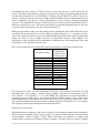
Applications of Data Analysis (EC969)
Simonetta Longhi and Alita Nandi (ISER)
Contact: slonghi and anandi; @essex.ac.uk
Week 3 Lecture 1: Gains from marriage and cohabitation
Input dataset: Week3Lecture1.dta
Do file: Week3Lecture1.do
I Research question
We want to estimate and compare the gains in economic well-being from marriage and
cohabitation for men and women in England. In other words, we want to estimate the effect
of marital status on household income (a measure of economic well-being) for men and
women. To identify this effect we will need to
(1) Compute household income that is comparable for single and multiple person households
(2) Control for other observable characteristics in the household income model that may be
correlated with marital status
(3) Account for any unobservable factors in the household income model that may be
correlated with marital status
The background paper for this exercise is Light (2004).
We thus want to estimate the parameters in the following model and based on those estimate
the economic gains from marriage and cohabitation.
Yit  f (0  1Marriedit  2Cohabitingit   x X it  q Ai  i   it )
(1)
where i (i=1,2,…n) represents individuals, t time (t=1,2,…T), Yit household income for
person i at time t and  i ,  the unobserved factors. X it , Ai are vectors of time-varying and
time invariant observed factors and Marriedit , Cohabitingit are 0-1 dummy variables
representing marital status.
Equivalised Household Income
Household income in a single person and multiple person households is not comparable in
terms of economic well-being because of sharing rules and economies of scale. In other
words, an individual’s economic well-being when living alone and when living in a two
person household with the same household income is not the same. First, in a multiple person
household the income is shared. As we do not know how the income is shared it is generally
assumed to be shared equally among all members. If the household income in a two
household is £1000, then each person in the two-person household has access to £500 only.
However, certain goods and services can be shared among different members, e.g., television,
apartment, cooking and other household activities. So, the individuals in the two-member
1|Week3Lecture1
household may have access to £1500 worth of goods and services in total and £750 per
person. Thus the actual difference between a person in the single person household and in the
two-person household is not (£1000-£500=) £500 but only (£1000-£750=) £250. Thus if we
want to compare the income between a single adult household and a two adult household, we
need to normalise the income of these households to that of some common household
structure. This normalised income is called equivalised income and the normalising factor is
known as equivalence scale. All scales must declare a particular household type as the base
or norm and the equivalence scale for such a household is 1.
Different equivalence scales exist depending on the assumptions they make about the extent
to which some goods and services can be shared by different people, i.e., economies of scale.
Also, some of the equivalence scales treat children differently from adults as they assume that
adults are likely to put a higher pressure on household resources than children. So,
equivalence scales are different for households of different sizes and composition. One such
equivalence scale is the McClements scale.
Here is the scoring rule used in the McClements Equivalence scale before housing costs.
McClements
Equivalence
Household member
Scales, before
housing costs
Head
0.61
Spouse
0.39
Other second adult
0.46
Third Adult
0.42
Further adult
0.36
Dependent child aged
0-1
0.09
2-4
0.18
5-7
0.21
8-10
0.23
11-12
0.25
13-15
0.27
16+
0.36
Source: Taylor et. al. (2010) Table 29, pp
App2-4
The equivalence factor for each household is the sum of the scores in the table for each
household type. For example, a couple with no children will have an equivalence scale of
0.61 (Head) + 0.39 (Spouse) = 1.0. In the BHPS the equivalence for each household is
computed using the table above and already provided with the dataset. Some of the other
most commonly used equivalence scales are OECD scale, US poverty line equivalence scale.
The implicit assumption is that the income is shared equally by all members, i.e., no member
has a greater claim to the household income than the others.
Household income model
Household income comprises of the sum of income of all earning members in the household.
These consist of earnings such as wages, profits, etc and non-earning income such as interest
and dividends, welfare receipts or gifts. When individuals get married or cohabit with
someone their economic well-being is likely to change as another person’s income is added,
2|Week3Lecture1
but the total income now needs to be shared between two persons and there are some gains
because of economies of scale (sharing one apartment, television, household chores).
If marriage or cohabitation were completely random events then we could estimate the
economic gains from marriage or cohabitation by regressing household income on marital
status. But there are some factors which may affect household income as well as marital
status, so we need to control for these. These are factors such as education, region of
residence, employment level, past labour market experience, marital status, presence of
children. For example, college graduates are expected to earn higher pay than those with only
O-level or A-level either as a reflection of their higher human capital accumulation or
signalling their higher ability. Education is also a determinant of marital status as educational
institutions serve as marriage markets and people may look for similar educational attainment
in their mates. Similarly, individuals working in London and other economically thriving
urban regions where there are more opportunities of higher paying jobs are likely to earn
higher pay. And these regions with their higher population density may also provide larger
marriage markets.
We thus want to estimate the parameters in the following model, specifically β1 and β2. Here
as in Light (2004) we have controlled for presence of children, age, hours worked, education,
current enrolment status, ethnicity and year. In addition we have also controlled for region of
residence.
log Yit  0  1Marriedit  2Cohabitingit  3 Re gionit 4 Anykidsit  5 Ageit
 6 Hoursworkedit  7 Educationit  8 Ethnicityi  9Yearit  i   it
(2)
Generally the model of log of income and not income itself is assumed to be linear. So, here
we have used log household income instead of household income.
Note Light (2004) also estimates the effect of the duration of marriage, single status or
cohabitation on household income. In this exercise we have ignored this.
(3) Estimation and unobserved factors
If the unobservables or the error terms, i and  it are not correlated with marital status, then
we can consistently estimate economic gains from marriage and cohabitation,  1 and  2 , using
Ordinary Least Squares (OLS) for (2). In other words, if marital status is endogenous to
household income then we cannot consistently estimate  2 and  3 using OLS. The reason is as
follows. OLS estimates these parameters by comparing the income of single persons with the
income of married and cohabiting persons. But if those who are single are different (but this
is not observed and so cannot be controlled for) from those who are married or cohabiting in
terms of their earnings potential then the OLS estimates of the economic gains from marriage
and cohabitation will merely reflects the differences in these earnings potentials. For
example, a woman who is highly motivated may search intensively for a spouse or partner
and as well as for a better quality job. Such a woman will be more likely to be married or
cohabiting as well as be in a high paid job. Suppose that if none of the men earn anything,
then if we compare single and married women we will find that the household incomes of the
latter are higher than the former and erroneously conclude that there are economic gains from
marriage/cohabitation.
3|Week3Lecture1
In this model we have hypothesised that the error term comprises of two parts – an individual
effect, i and a time varying component,  it . Other terms used to describe this individual
effect are unobserved component, latent variable, unobserved heterogeneity, individual
heterogeneity. If we assume that i is correlated with marital status but  it is not, then we can
consistently estimate  1 and  2 using first difference or fixed effect methods. These methods
aim to eliminate the individual specific fixed effects and use the within individual changes in
income and marital status to estimate  1 and  2 .
Fixed Effect Method
This method involves subtracting the across-time mean of a variable from the value at any
point in time (fixed effect transformation or within transformation) and estimating the
resulting differenced equation by OLS. The differenced equation is as follows:
 log Yit  1Marriedit  2Cohabitingit  3 Re gionit 4Anykidsit  5Ageit
 6Hoursworkedit  7Educationit  9Yearit   it
(3)
1 T
 log Yis and T is the total number of time periods observed and
T s1
similarly for all other variables.
where  log Yit  log Yit 
First Difference Method
In this method we take the difference of each variable between two time points (first
differencing transformation) and estimate the resulting differenced model using OLS. The
differenced equation is as follows:
 log Yit  1Marriedit  2Cohabitingit  3 Re gionit 4Anykidsit  5Ageit
 6Hoursworkedit  7Educationit  9Yearit   it
(4)
where  log Yit  log Yit  log Yi (t k ) and similarly for all other variables and k (the time
difference is the same for all observations).
As you can see the effect of i is eliminated in both estimation methods. So, even if i is
correlated with marital status, OLS will yield consistent estimates of  1 and  2 . Also note any
time invariant regressor will also be eliminated and we will not be able to estimate its
coefficient using these methods. More generally, we will only be able to estimate parameters
of those variables which change for at least some individuals and so the coefficients are
estimated only on the basis of those cases where these variables have changed. You can use
xttab and xtsum commands to identify time varying and time-invariant variables (more in
section II).
What would happen if in our dataset there were hardly any individuals (or none at all) whose marital
status changed?
Stata code to estimate a model using fixed effect method is:
xtreg depvar indepentvar, fe
4|Week3Lecture1
But to use this and any other xt commands such as xttab and xtsum (i.e., commands that
start with xt) we first need to set up the data as a panel dataset, i.e., xtset the data. In this
Stata command you tell Stata which is the individual identifier (idvar) and which is the time
identifier (timevar).
xtset idvar timevar
For the first difference mode we need to compute the first differences. We can do that easily
in Stata once Stata knows this is a panel dataset (i.e., after we have xtset the data).
generate diffdepvar
= D1.depvar
generate diffindepvar = D1.indepvar
Estimate first difference estimator by simply running OLS on the differenced data
regress diffdepvar diffindepvar
First difference Vs fixed effects methods
These methods yield the same estimates when T=2, but not always when T>2. Fixed effects
estimator is more efficient than the first difference estimator if the time-varying error
component  it is homoskedastic and serially uncorrelated. The first difference estimator
yields more efficient estimates under less strict conditions; it only requires the first difference
of the error term to be serially uncorrelated and homoskedastic. So, suppose the time-varying
error component is a random walk, i.e., serially correlated as follows:
 it   it1  it
where  it is white noise, i.e., a normal variable with zero mean and variance one. Then  it is
not serially correlated and so the first difference method yields efficient estimators.
Random effects model
Random effects estimator is consistent only if the unobserved heterogeneity is not correlated
with the independent variables. Under this assumption estimating the model in (2) using OLS
will also yield consistent estimators but not the most efficient; random effects estimator will
be more efficient. This is because the random effects estimator is computed using using
generalized least squares (GLS) or rather feasible GLS (FGLS) which takes into account the
serial correlation in the error structure i   it .
In Stata, the code to estimate the model using Random Effects using Feasible Generalized
Least Squares is
xtreg depvar indepentvar, re
In Stata, the code to estimate the model using Random Effects using MLE is
xtreg depvar indepentvar, mle
Why and when to use random effects?
If the independent variables are not correlated with the individual effect then we can use both
random and fixed effects and get consistent estimates of the coefficients. However, if this
assumption does not hold then only fixed effect methods and FD methods yield consistent
estimates. So, we can construct a Hausman test to determine which method to use. Random
5|Week3Lecture1
effect has another advantage over fixed effects methods: we can estimate the coefficients of
time invariant variables.
In Stata, the command hausman performs the Hausman’s specification test. To use the
command we have to:
1. Estimate the model that is consistent whether or not the hypothesis is true
2. Store the estimation results of the first model (consistent_estimate)
3. Estimate the model that is efficient (and consistent) under the hypothesis that you
are testing, but inconsistent otherwise
4. Store the estimation results of the second model (efficient_estimate)
5. Use: hausman consistent_estimate efficient_estimate
to perform the test
In our specific case the consistent_estimate will be the fixed effects model, while the
efficient_estimate will be the random effect model. You can use the same command to
perform other kinds of test. Just make sure that the first set of results is the consistent one
and the second set of results is the efficient one. Remember: “always consistent” first and
“efficient under H0” second.
Robust estimators
If observations are independently but not identically distributed then using vce(robust)
option produces consistent standard errors. If observations are distributed independently
across clusters but not independently within clusters then using vce(cluster clustervar)
produces consistent standard errors.
If there is heteroskedasticity or within-panel serial correlation in the time-varying error
component  it then we should use the vce(robust) or vce(cluster panelvar) option to
get Huber/White or sandwich robust standard errors. Both yield the same result: “Clustering
on the panel variable produces an estimator of the VCE that is robust to cross-sectional
heteroskedasticity and within-panel (serial) correlation that is asymptotically equivalent to
that proposed by Arellano (1987).” Stata Help
xtreg depvar indepentvar, fe vce(robust)
xtreg depvar indepentvar, fe vce(cluster panelvar)
II Setting up the data
As you have realised the data needs to be in long format. We have provided the long form
dataset (pid is the unique person identifier and wave is the interview year or time identifier).
The dataset is called Week3Lecture1.dta. In the model above we have suggested some
independent variables that are likely to affect household income. This dataset contains all the
variables needed for the above model. If you would like to include others, you will need to
extract those separately from the BHPS data files and merge with this dataset.
Examine the data. Use any or all of these: describe, inspect, tabulate, summarize
6|Week3Lecture1
BHPS data does not have any system missing. Instead, all missing values are assigned
negative values (e.g., -1 for don’t know, -8 for not applicable, see documentation for the
complete list). Stata will not recognize these as missing values. So, we need to recode these
to missing.
Set all missing values to system missing. Hint: use mvdecode or recode
First we need to compute the dependant variable. Note the income is in nominal terms and so,
we need to deflate the income by a price index. One such price index is the “implied GDP
deflator” (name of the variable in the dataset is deflator). It is the GDP calculated at the
current prices divided by the GDP calculated at the prices for some given year. This variable
is not included in the BHPS but we have provided it using the Blue Book 2009 produced by
the Office of National Statistics.
Compute the equivalised household income.
Compute the real equivalised household income.
Compute the log of real equivalised household income
Next, we need to create the independent variables. The dataset has these variables, not
necessarily in the format that we want to use. All categorical variables need to be transformed
into 0-1 dummy variables to be included. For example, highest educational attainment
variable (edu_highest) has five categories. We need to create four 0-1 dummy variables for
the four categories (the fifth one is the omitted category). And easy method to create 0-1
dummies from a categorical variable is as follows:
tab var, gen(newvar)
If var had n categories then this will create n 0-1 dummies called newvar1-newvarn.
When you are thinking of transforming the existing variables into new ones (that you need
for your estimation) check the variable label and value labels of the variables. Also, if there
are categorical variables, then you may want to reduce the number of categories so that none
of the categories has too few observations and the categories reflect what you want to say.
For example, if you are interested in seeing the difference between people living in London
vis-à-vis other areas but the region variable has 19 categories, then you should collapse all
categories into just two – London and other than London.
The variables that we need for the analysis are:
(1) Married, Cohabiting
(2) Region of residence: Collapse into fewer categories?
(3) Any children present in the household?
(4) Hours worked
(5) Education
(6) Age: And some of its polynomials, say age-squared?
(7) Time/year dummies
(8) Living with at least one parent?
(9) Ethnicity: Collapse into fewer categories?
7|Week3Lecture1
(10) Currently enrolled in school?
Now the dataset is ready.
Examine the final data set. Again use any or all of these: summarize, describe, inspect,
tabulate.
But with a panel data set we can see the data patterns better if we use some of the xt
commands. “The xt series of commands provide tools for analyzing panel data (also known
as longitudinal data or in some disciplines as cross-sectional time series when there is an
explicit time component)” (From Stata Help)
First we need to tell Stata that this is a panel dataset and which variable identifies the person
and which variable identifies the time variable
xtset pid wave
You can use xtdescribe to see what this panel data looks like in terms of whether it is a
balanced or unbalanced panel, what percentage of observations have a particular pattern of
occurring in the dataset. See what Stata has to offer.
Which of the variables do not vary with time? Hint: Use xtsum and xttab
Sample selection
Our population of interest is England and so,
keep if region<17
The dataset consists of those who were interviewed face-to-face (i.e., in person) or via
telephone or by proxy (when someone else answered from them). Studies show that
sometimes how people respond to a question varies by who answers the question and the
interview mode. So, we have decided to drop all those cases who were not interviewed facefo-face. IVFIO is one for those who were interviewed face-to-face.
keep if ivfio==1
While Light (2004) includes those who are currently enrolled it may not be a good idea for
us. The reason is as follows. In her paper she has computed the household income for just the
person and his/her spouse/partner if present. However, we have used the BHPS provided
household income which includes the income of all household members. In case of students
the other household members could be their roommates. So, it would be a good idea to drop
those who are currently enrolled.
keep if enrolled==0
III Estimation
Estimate the effect of marital status on household income using pooled OLS, fixed effect and first
difference methods. Do this for men and women separately.
Compare the estimated gains from marriage by each of these methods. Which one yields the greatest
estimate of the gains from marriage?
8|Week3Lecture1
Based on any one of the estimators answer the following:
What is the estimated gain from marriage for men and women?
Is the gain from marriage higher or lower than that from cohabitation for men?
Is the gain from marriage higher or lower than that from cohabitation for women?
What is the estimated value of the coefficient for ethnicity variable?
Why is year 1991 omitted from the first difference estimation?
Stata conducts an F-test for the Null Hypothesis that unobserved effect is zero (or constant
for everyone). sigma_u and sigma_e are the estimated variance for the unobserved effect,  i ,
and the time-varying error term,  it , and rho is the fraction of the total variance that is
explained by variation in  i . You can see the results at the bottom of the output following
fixed and random effects estimation.
Are unobserved effects zero for men? Are these zero for women?
Next, the Random Effects Estimator
Estimate the model using random effects, separately for men and women.
What is the estimated value of the coefficient for ethnicity variable?
Should we use the Random Effects or Fixed Effects estimator?
Using a Hausman test do you think we should use the Random Effects or the Fixed Effects model?
There may be heteroskedasticity or within-panel serial correlation in the time-varying error
component.
What would you do to produce correct estimates of standard errors for a first difference, fixed effect
and random effects estimator that is robust against heteroskedasticity or within panel serial
correlation?
Reference:
Light, Audrey. 2004. “Gender Differences in the Marriage and Cohabitation Income
Premium” Demography, 41(2): 263-284.
Taylor, Marcia Freed (ed). with John Brice, Nick Buck and Elaine Prentice-Lane (2010)
British Household Panel Survey User Manual Volume A: Introduction, Technical Report and
Appendices. Colchester: University of Essex.
Wooldridge, Jeffrey. 2001. Econometric Analysis of Cross-sectional and Panel Data. MIT
Press
9|Week3Lecture1
[Optional] How to create dataset Week3Lecures1.dta
This consists of data from different BHPS data files: (i) individual respondent data collected
from all waves (windresp), (ii) household sample file from all waves (whhsamp), (iii)
household response files from all waves (whhresp), (iv) household grid information from all
waves (windall) and (v) time invariant (fixed) individual level data collected (xwavedat).
Data from these three files have been merged together.
If you wanted to create these yourself, here is a guide to do that. See
Week3Lecture1_dataprep_DoFile.pdf which contains the corresponding do file for this.
For each wave do steps 1-5:
1. Get information about the individual that was asked in the individual questionnaire from
windresp.dta: employment status, enrolment status, highest educational qualification, work hours,
weight, region of residence
2. Get other information about the individual that was coded from the household grid from
windall.dta: marital status, person number of spouse, father and mother, age, number of own children
in the household, interview outcome
3. Get information on strata and primary sampling unit from whhsamp.dta
4. Get information about the household that was asked in the household questionnaire from
whhresp.dta: monthly household income, McClement’s scale, household size, number of children in
the household
5. Merge all these datasets sequentially for each wave, keep only those observations present in all
datasets. Points to remember about merging:
 Datasets being merged should be sorted on the variable or variables that are being used to
merge these
 Check _merge to see how many cases were available in both, how many in only one
 _merge is created by Stata at every merge and so if you don’t drop _merge or rename it to
something else after each merge, Stata will produce an error message saying “_merge
already exists” and will not allow you to perform merge until you have dropped _merge or
renamed it.
In addition to these variables always remember to include the appropriate unique identifiers in each of
the datasets – pid, hid & pno.
6. Now using a foreach loop create a dataset for all waves in the long form (as in week 1).
7. Get information about gender, race/ethnicity and sample origin from xwavedat.dta and merge this
with the long form dataset in step 6 – keep only those present in both datasets.
8. Create the following variables
(i) Create a 0-1 dummy variable that takes on 1 if currently employed using JBHAS (did paid work
last week) and JBOFF (no work last week but has job)
(ii) Hours worked variable which is zero for all those who are not employed using employed dummy
created in (i) and JBHRS
(iii) Create a categorical variable for highest qualification using QFEDHI.
(iv) Create a 0-1 dummy variable if individual is currently enrolled in school or further education
(v) Create a categorical variable to represent the country of residence using REGION.
(vi) Create a variable that captures the implicit GDP deflator for each year/wave.
Finally change value labels to make them consistent with variable names and if you want keep only
those that are necessary for the subsequent analysis.
9. Sample selection: drop the ECHP sub-sample
10 | W e e k 3 L e c t u r e 1