Download SpecPro User Manual

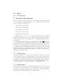
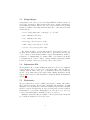
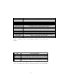
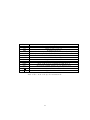
SpecPro User Manual
Dan Masters
October 3, 2011
Contents
1 Program overview
2
2 Download and Installation
2
3 Modes
3.1 Standard Version . . .
3.2 Small Version . . . . .
3.3 Basic Version . . . . .
3.4 The “space” keyword .
.
.
.
.
.
.
.
.
.
.
.
.
.
.
.
.
.
.
.
.
.
.
.
.
.
.
.
.
.
.
.
.
.
.
.
.
.
.
.
.
.
.
.
.
.
.
.
.
.
.
.
.
.
.
.
.
.
.
.
.
.
.
.
.
.
.
.
.
.
.
.
.
.
.
.
.
.
.
.
.
.
.
.
.
.
.
.
.
.
.
.
.
.
.
.
.
2
2
2
3
3
4 The
4.1
4.2
4.3
4.4
4.5
4.6
4.7
.
.
.
.
.
.
.
.
.
.
.
.
.
.
.
.
.
.
.
.
.
.
.
.
.
.
.
.
.
.
.
.
.
.
.
.
.
.
.
.
.
.
.
.
.
.
.
.
.
.
.
.
.
.
.
.
.
.
.
.
.
.
.
.
.
.
.
.
.
.
.
.
.
.
.
.
.
.
.
.
.
.
.
.
.
.
.
.
.
.
.
.
.
.
.
.
.
.
.
.
.
.
.
.
.
.
.
.
.
.
.
.
.
.
.
.
.
.
.
.
.
.
.
.
.
.
.
.
.
.
.
.
.
.
.
.
.
.
.
.
.
.
.
.
.
.
.
.
.
.
.
.
.
.
.
.
.
.
.
.
.
.
.
.
.
.
.
.
3
3
4
4
4
6
6
6
Interface
Navigating Data . .
Setting the Redshift
Stamp images . . . .
1-D Spectrum . . . .
2-D Spectrum . . . .
Re-extracting 1-D . .
SED . . . . . . . . .
.
.
.
.
.
.
.
5 Cross-correlation
7
6 Output
6.1 Redshift results . . . . . . . . . . . . . . . . . . . . . . . . . . . .
6.2 Images . . . . . . . . . . . . . . . . . . . . . . . . . . . . . . . . .
6.3 1-D spectrum . . . . . . . . . . . . . . . . . . . . . . . . . . . . .
7
7
8
8
7 Required data formats
7.1 1D Spectrum . . . .
7.2 2D Spectrum . . . .
7.3 Stamp Images . . . .
7.4 Information File . .
7.5 Photometry . . . . .
8
8
8
9
9
9
.
.
.
.
.
.
.
.
.
.
.
.
.
.
.
.
.
.
.
.
.
.
.
.
.
.
.
.
.
.
1
.
.
.
.
.
.
.
.
.
.
.
.
.
.
.
.
.
.
.
.
.
.
.
.
.
.
.
.
.
.
.
.
.
.
.
.
.
.
.
.
.
.
.
.
.
.
.
.
.
.
.
.
.
.
.
.
.
.
.
.
.
.
.
.
.
.
.
.
.
.
.
.
.
.
.
.
.
.
.
.
.
.
.
.
.
.
.
.
.
.
.
.
.
.
.
1
Program overview
SpecPro is designed to show the user all available information about a spectroscopic target, including stamp images and source SED. Spectroscopic targets in
modern, multiwavelength survey fields have this extra data available and it can
be very helpful in trying to decipher confusing or faint spectra.
The interface displays the 1-D spectrum, 2-D spectrum, source SED, and an
arbitrary number of stamp images. It lets the user interact with the data in a
variety of ways to characterize the source and determine redshift.
Note that the interface does not require that all of this data is available,
and can be used if, for example, only the 1-D spectrum is available, or there is
no spectral data and the user just wants to examine stamp images/SED. Thus
it can be a powerful tool even if only spectroscopic data (or only photometric
data) is available. However, it is at its most powerful when photometric and
spectroscopic data are examined together.
The formats are simple and general, so that data from any instrument/survey
can easily be adapted to view with the program.
2
Download and Installation
The code and installation instructions are available at http://specpro.caltech.edu.
You must have the IDL Astronomy User’s Library to use SpecPro. This library is maintained at NASA GSFC by Wayne Landsman and can be found
here. The automated cross-correlation capability of SpecPro relies on the IDL
routines mpfit.pro, mpfitpeak.pro, and mpfitfun.pro, written by Craig Markwardt. These can be downloaded here.
3
3.1
Modes
Standard Version
The standard mode of SpecPro is invoked at the IDL command line by typing
specpro, [slit number]
as the IDL command line. It is the default mode, and launches a large interface displaying 11 stamps, the 1-D and 2-D spectrum, and the source SED.
If any of this information is missing, the relevant windows are left blank.
3.2
Small Version
The standard mode of the interface may be too large for some monitors. If this
is the case for you, launch the program with the keyword /small, by typing
2
specpro, [slit number], /small
at the IDL command line.
3.3
Basic Version
Realizing that you may either not have the photometric data for the program,
or may wish to use it only as a quick way of examining spectra, we provide a
basic mode in which only the spectral data is dislayed. This is invoked by typing
specpro, [slit number], /basic
at the command line.
3.4
The “space” keyword
If the spectrum you are looking at was taken in space (e.g. a WFC3 grism
spectrum) you can use the keyword “space” to prevent sky bands from being
plotted. For example,
specpro, [slit number], /space
4
The Interface
The interface consists of the data displays as well as widgets allowing you to
perform various tasks, such as navigate through spectra in the mask directory,
adjust the current redshift guess, bin and smooth the 1D spectrum, overlay
galaxy templates, plot the redshifted positions of common emission and absorption features, change stamp image and 2D spectrum contrast, and save results
to an external file. In the following sections we describe the elements of the display and discuss the ways of interacting with it. Most of the interactive parts
of the display should be obvious from playing with the interface, and there is a
short tutorial available on the download website to provide an overview.
4.1
Navigating Data
As explained in Section , the working directory should contain the data to be
examined. SpecPro expects the data within the directory to be differentiated
by slit number, although any unique indexing scheme can be used. When the
program is launched with the command
specpro, [slit number]
3
the program looks for the relevant files corresponding to this slit number. The
program can also be launched with no slit number. In this case, the interface
loads (empty) and waits for you to enter a slit number in the text box in the
upper left. Once in SpecPro, you can navigate between different slit numbers
using the “Previous” and “Next” buttons in the upper left, or by typing the
desired slit number in the text box and pressing return.
4.2
Setting the Redshift
You can manually play with the current redshift guess. To do this, type a
redshift in the “Enter redshift guess:” field in the upper left and press return.
Alternatively, adjustments can be made to the current redshift with the arrow
buttons located beneath the text box.
4.3
Stamp images
Available stamp images of the source are displayed on the left side of the interface in 100x100 pixel windows. Under the final window is a scroll list containing
the names of overflow images. You can click entries in this list to display them
in the final stamp window, allowing an effectively arbitrary number of stamp
images to be stored and viewed with the interface. The images are displayed in
the order in which they are stored in the structure array.
The displayed images are S/N plots generated by dividing the image flux by
the average error in the image. This maximizes the dynamic range. By viewing
the stamps you can quickly determine the source of a serendipitous spectrum
and whether photometric points in the source SED correspond to real detections
or artifacts.
Selecting the “Show extraction” button (located underneath the 2D plot
window) causes the scale in arcseconds to be displayed on the stamps. If the slit
information (RA, DEC, length, width, and angle) is provided in the information
file, clicking this button will cause the slit to be plotted over the stamp images.
The contrast of the images can be adjusted with a slider widget in the lower
left of the interface.
4.4
1-D Spectrum
The 1-D spectrum is displayed in the upper right window of the display. The
spectrum itself is in white, with overlaid spectral templates displayed in blue.
Regions of significant atmospheric absorption are indicated with horizontal blue
lines. Table 1 summarizes the absorption regions that have been marked. The
residual error can be overlaid on the plot by clicking the “Show error” button
on the second row down from the 1D display.
The 1-D spectrum can be binned and smoothed to bring out features in
low S/N spectra with the “Bin” and “Smooth” droplists under the 1-D display.
Binning combines pixels, reducing the resolution of the spectrum to increase
the S/N, while smoothing performs an inverse variance weighted average in the
4
Feature
B band
A band
Water
Water
O2
Water
CO2
CO2
Water
CO2
CO2
Wavelength Region
6864-6945 Å
7586-7708 Å
9200-9700 Å
1.10-1.16 µm
1.25-1.28 µm
1.34-1.45 µm
1.57-1.58 µm
1.60-1.62 µm
1.79-1.97 µm
2.00-2.03 µm
2.04-2.07 µm
Table 1: Regions of strong atmospheric absorption marked in SpecPro.
vicinity of each pixel to reduce the noise. Note that the binning and smoothing are just for you visual benefit and do not influence the cross-correlation
calculation.
The “Template:” droplist next to the bin and smooth widgets lets you choose
from among a variety of spectral templates to overlay on the 1-D spectrum.
When one of these is selected, cross-correlation is automatically performed, and
the six best redshift solutions are computed, with the best solution set as the
current redshift guess. Alternate auto-z solutions can be selected for examination from the droplist “Select auto-z solution”. Once the cross-correlation
has been performed, you are free to manually adjust the redshift to move the
template around, if you think the cross-correlation has returned incorrect answers. The scaling of the template can be adjusted with the “Template scaling:”
droplist, to provide a better visual comparison with the spectrum. Auto-z can
be turned off with the “Auto-z OFF” button.
The “Auto center” button performs cross-correlation with the currently selected galaxy template in a small region (z±0.05) around the current redshift
guess. This can help zero in on the correct answer when you know you are close
but don’t want to manually adjust the redshift to the exact value.
Common emission/absorption lines from different galaxy types can be overlaid at the observed-frame positions by clicking on the buttons in the second
row down from the 1-D display. This also causes the lines to be displayed over
the 2-D spectrum.
Finally, the 1-D display can be zoomed on by drawing a box with the mouse
around the region of interest (no box actually appears). Just click, drag and
release to see the zoomed region. Reset the zoom using the button on the second
row down from the 1-D display.
5
4.5
2-D Spectrum
The 2D spectrum is displayed beneath the 1D spectrum, and is binned, if necessary, to fit the display. The contrast of the 2D spectrum can be adjusted with
a slider widget. Next to the contrast slider is a droplist widget labeled “Max
sigma:”. This is set to 10 by default, which indicates that contrast scaling has
an upper limit of 10σ, so that pixels 10σ from the mean are rescaled to the
maximum pixel value of 255. Lowering this value can help in cases in which the
spectrum of interest is being drowned out by the light of bright serendipitous
sources.
The positions of significant atmospheric absorption features are indicated
with horizontal red lines above and below the spectrum. The “Show extraction”
button, located under the 2-D display, cause white lines to appear indicating
the region in which the 1-D spectrum has been extracted from the 2-D.
Note that the 2-D can be zoomed in the same manner as the 1-D, but in
the case of 2-D this causes an unbinned plot of the zoom region to apear in a
separate window. Double clicking either the 1-D or the 2-D displays prompts
you save a .tif image of the display.
4.6
Re-extracting 1-D
You can reextract the 1-D from the 2-D, which can be useful for dealing with
serendipitous sources. To reextract, place the cursor over the 2D spectrum at
the vertical position desired, then click, drag horizontally (by any amount, in
either direction) and release. This triggers the reextraction, and when it is
complete the 1D plot is updated with the newly extracted spectrum. The width
of the region used to extract the 1D spectrum is determined by the value of
extractwidth, a parameter in the information file described in Section 3.4. If
this parameter is not in the information file a default width of 10 pixels is used.
A dialog box lets you save the reextracted spectrum as a .fits file.
4.7
SED
The source SED is displayed in the bottom right window of the interface. The
information for this plot comes from the photometry file, described in Section
3.5. The plot extends from 1000 Å to 10 µm and displays photometric AB magnitudes with errors. The effective widths of the photometric bands are indicated
with horizontal bars and errors in the magnitude estimates are indicated with
vertical bars. Observed-frame positions of important SED features are indicated
with vertical blue lines. These features include the Lyman limit at 912 Å, Lyα
at 1216 Å, the 4000 Å break, and the typical SED peak of evolved galaxies
at 1.6 µm. The wavelength coverage of the spectrum is indicated with green
vertical lines.
6
5
Cross-correlation
Automated redshift determination by convolution against spectral templates is a
powerful and time-saving capability. We have adapted cross correlation routines
originally written for the SDSS spectral reduction package for use in SpecPro,
with a library of spectral templates available to cross correlate against (see
Table 2). The templates currently available span a broad range of galaxy types
and also include some stellar templates (stellar templates, particularly of brown
dwarfs, can help identify high-redshift selected sources that spectroscopy reveals
to be stars). The droplist labeled “Template:” underneath the 1D spectrum
lets you select the template to overlay on the spectrum. You are expected to
be able to choose an appropriate template based on the spectrum and other
information about the source. When one of the galaxy templates from this list
is selected, the six best redshift matches are computed and the best solution is
displayed. The droplist “Auto-z solution:” under the 1D spectrum contains all
of the solutions for examination. Clicking an alternate solution will switch to
the new redshift guess and move the template accordingly. Because the spectral
template is overplotted on the 1D spectrum, the correctness of the result can be
easily verified. The scaling of the template can be adjusted via the “Template
scaling:” button to provide a better visual match to the spectrum.
In some cases the cross correlation fails to find the solution, even though
the correct answer is apparent to the user. In this case the redshift can be
adjusted manually to find the answer, but finding the exact solution can be
time consuming. Therefore we added an “Auto center” button that computes
the cross correlation solution against the currently selected galaxy template in
a small region (z ± 0.05) around the current redshift guess.
6
6.1
Output
Redshift results
To the left of the SED plot window are four output fields with which the user
can save the redshift, a confidence associated with it, their initials, and notes
on the spectrum. The output values can be saved to file by clicking the “Save
Redshift” button. The output is saved in ascii format and contains the mask
name, source name, slit number, RA, and DEC as well as the redshift result.
Results are always appended to the end of the selected output file and multiple
entries for a single source can be added. Once an output file has been selected,
it will be the default output location for the rest of the SpecPro session.
To the right of the “Save Redshift” button is the button “Save Spec1D”.
This saves the displayed 1D spectrum (wavelength and flux at the current zoom,
bin, and smooth level) to an ascii file for plotting in other programs. Note that
under the 2D spectrum are buttons “Like z” and “No z”, the purpose of which
is to quickly populate the redshift output field once the redshift - or inability to
find one - has been determined.
7
6.2
Images
6.3
1-D spectrum
7
Required data formats
We have attempted to make the required formats simple and straightforward
so that data from any instrument/survey can be readily adapted for use with
SpecPro. SpecPro accepts five files:
• The 1D spectrum file (fits)
• The 2D spectrum file (fits)
• The stamp image file (fits)
• The photometry file (ascii)
• The information file (ascii)
While the files are expected to be arranged by slit number, any sequential
numbering scheme can be used. None of the five files listed is actually required
for the program to run; if one is missing, the corresponding field in the interface
is left blank.
The adopted name convention for each file is given in Table 3. The names
have a leading descriptor giving the file type, followed by the mask name, the
slit number, the target name, and the extension, all separated by periods. A
few points are worth noting. First, the mask name and target name can be set
to dummy values; only the slit number is used by the program. Second, the slit
number is expected to be three characters long, so that slit 30 would be saved
with the slit number 030. Finally, there should not be any periods used in the
mask name or the target name.
7.1
1D Spectrum
The 1D spectrum is a stored as a structure with three fields: flux, ivar, and
lambda. Each field holds a one-dimensional double array. The flux field is the
spectrum, the ivar field is the inverse variance of the flux, and lambda is the
wavelength at each pixel, in angstroms. Note that the units of flux are arbitrary,
but values proportional to Fν are preferable because this matches the units of
the spectral templates. The structure must be saved in FITS format.
7.2
2D Spectrum
The 2D spectrum is also stored in a structure with the three fields flux, ivar, and
lambda. However, each field here is a two-dimensional double array, including
the lambda field, which contains the wavelength solution for each pixel in the
2D spectrum. The 2D spectrum is stored in FITS format.
8
7.3
Stamp Images
Stamp images of the source are stored in a single FITS file, with the data stored
as an array of structures. Each element in the array contains a stamp image
and ancillary information, with the size of the array determined by how many
stamps are available. The stamp structures must all be of the same form, with
fields as follows:
• name - string giving name of the image, e.g. “U band”
• flux - 100x100 double array
• ivar - 100x100 double array
• RA - image center in degrees, double
• DEC - image center in degrees, double
• pixscale - arcseconds per pixel, double
The stamps should be oriented with north up. If the inverse variance for
the image is not available then it should either be approximated in some way
or set to all zeros. If the stamp is smaller or larger than 100x100, it should be
resampled to be 100x100 using, for example, IDL’s congrid function. It should
be straightforward to write a routine to package available stamp images in this
format; an example of such a program is provided on the website.
7.4
Information File
The information file contains ancillary information about a source displayed
by the interface and/or used in some of its functionality. The file has two
columns, with the name of the piece of information in the left column and
the the corresponding value in the right column. Missing information should
indicated with a value of 0. The information contained in this file is summarized
in Table 4.
7.5
Photometry
The photometry file is a space delimited file with five columns: filter name,
filter central wavelength, effective filter bandwidth, AB magnitude, and AB
magnitude error. Both the filter central wavelength and effective filter bandwith
should be expressed in angstroms. Non-detections should be indicated with an
AB magnitude of -99, and the AB magnitude error should be set to the lower
bound on the AB magnitude established by the non-detection.
Examples of all of these files are available on the program website and should
prove useful as templates for prospective users.
9
Template
VVDS LBG
VVDS Elliptical
VVDS S0
VVDS Early Spiral
VVDS Spiral
VVDS Starburst
SDSS Quasar
Red Galaxy
Green Galaxy
Blue Galaxy
LBG Shapley
SDSS LoBAL
SDSS HiBAL
A0-M6
Description
Lyman-break galaxy template from the VIRMOS-VLT Deep Survey
Passive galaxy template, strong absorption, no emission
S0 classification template, weak emission, absorption
Stronger emission, less absorption
Typical spiral spectrum, with strong emission features
Extremely strong nebular emission features
Typical broad-line quasar spectrum from the Sloan Digital Sky Survey
Passive galaxy template from PEGASE spectral evolution model
Early spiral/spiral template from PEGASE
Spiral/Starburst template from PEGASE
Lyman-break galaxy template from Shapley 2003
Low-ionization broad absorption line (BAL) quasar template
High-ionization BAL quasar template
Stellar templates from the Pickles catalog
Table 2: Summary of the spectral templates available for autocorrelation in
SpecPro.
File
1D spectrum
2D spectrum
Stamp images
Photometry
Information
Name Convention
spec1d.[mask name].[3 digit slit number].[target name].fits
spec2d.[mask name].[3 digit slit number].[target name].fits
stamps.[mask name].[3 digit slit number].[target name].fits
phot.[mask name].[3 digit slit number].[target name].dat
info.[mask name].[3 digit slit number].[target name].dat
Table 3: File name conventions for SpecPro. The mask name and target name
can be set to dummy values. The program differentiates files only by slit number.
10
Name
ID
RA
DEC
extractpos
extractwidth
slitRA
slitDEC
slitlen
slitwid
slitPA
zphot
zpdf
zpdf low
zpdf high
Description
Integer (can be set to dummy value)
Right ascension (degrees)
Declination (degrees)
Vertical extraction position (in pixels) of the 1D from the 2D spectrum
Width (in vertical pixels) of 1D extraction from 2D; used in reextraction
Central RA of slit, in degrees
Central DEC of slit, in degrees
Length of slit, in arcseconds
Width of slit, arcseconds
Angle of slit, in degrees (90 indicates EW aligned)
Photometric redshift estimate; used as initial z guess
Median redshift from probability density function
Lower bound on redshift
Upper bound on redshift
Table 4: The content of the SpecPro information file.
11