Download Computer Controlled Experimental Setup for Selective Excitation of

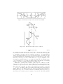
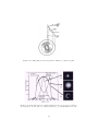
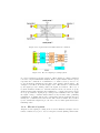
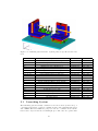
Computer Controlled Experimental Setup for
Selective Excitation of Mode Groups
- Software Pedro Filipe da Costa Teixeira
February 16, 2005
Abstract
Mode group diversity multiplexing uses each mode group as an independent
transmission channel over a multimode fibre. The division in different group
modes is based on selective excitation of mode groups. Studies on this technique require very accurate spatial launching conditions, where a computer controlled motorized setup provides the necessary high repeatability indispensable
to achieve reliable experiment conditions and results. The aim of this project is
then to implement a computer controlled motorized setup that satisfies mainly
the desired accuracy, repeatability and resolution. To do so, a software application for a common computer is developed in Labview programming. It is
capable of controlling relative positions of several optical components according
to the optical setup specific details and requests by translation of movement
stages. This software will establish a computer-controller communication. The
computer transmits simple commands which the controller decodes and executes by controlling stages movements. This process is transparent for the user,
which only has to input some optical system parameters and desired launching
conditions. The software will automatically calculate the correspondent necessary movements and confirm that they are performed. The program can realize
other features as free and independent stages movements or position information. The software can be used in different setups as setup system parameters
are user-defined.
Contents
1 Introduction
1.1 Project’s Context . . . . . . . . . . . . . . . . . . . .
1.2 Optical Principles and Concepts . . . . . . . . . . .
1.2.1 Snell’s Law . . . . . . . . . . . . . . . . . . .
1.2.2 Lenses . . . . . . . . . . . . . . . . . . . . . .
1.2.3 Numerical Aperture . . . . . . . . . . . . . .
1.2.4 Modes . . . . . . . . . . . . . . . . . . . . . .
1.2.5 Mode Dispersion . . . . . . . . . . . . . . . .
1.2.6 Ray Propagation in Multimode Graded Index
1.3 Mode Group Diversity Multiplexing . . . . . . . . .
1.3.1 Optical transmission system . . . . . . . . . .
1.3.2 Electrical system . . . . . . . . . . . . . . . .
1.3.3 Implementation . . . . . . . . . . . . . . . . .
2 Computer Controlled Setup System
2.1 Launching System . . . . . . . . . .
2.1.1 Collimating and Focusing . .
2.1.2 System Adjustment for Angle
2.1.3 Stage Movements . . . . . . .
.
.
.
.
.
.
.
.
.
.
.
.
.
.
.
.
.
.
.
.
.
.
.
.
2
2
2
2
3
5
5
10
10
14
14
15
16
. . . . . . . . . . . . . . .
. . . . . . . . . . . . . . .
and Offset Requirements
. . . . . . . . . . . . . . .
.
.
.
.
17
18
19
19
20
. . . .
. . . .
. . . .
. . . .
. . . .
. . . .
. . . .
Fibers
. . . .
. . . .
. . . .
. . . .
.
.
.
.
.
.
.
.
.
.
.
.
3 Automatic Control System
22
3.1 Hardware Description . . . . . . . . . . . . . . . . . . . . . . . . 22
3.1.1 Controller . . . . . . . . . . . . . . . . . . . . . . . . . . . 22
3.1.2 DC actuators . . . . . . . . . . . . . . . . . . . . . . . . . 24
4 Developed Software Tool
25
4.1 LabView . . . . . . . . . . . . . . . . . . . . . . . . . . . . . . . . 25
4.2 User Interface . . . . . . . . . . . . . . . . . . . . . . . . . . . . . 25
4.3 Block Diagram: Programming . . . . . . . . . . . . . . . . . . . . 27
5 Results and Conclusions
32
5.1 Improvements . . . . . . . . . . . . . . . . . . . . . . . . . . . . . 33
1
Chapter 1
Introduction
1.1
Project’s Context
The advent of telecommunications networks in the last decades has led to the
need of providing high bandwidth closer to the end user, at residential areas
traditionally served by copper wire and coaxial cable. Optical fiber presents
numerous advantages compared to the traditional media, such as larger bandwidth, lower losses and complete transparency to protocol and signal format.
In particular, polymer optical fiber (POF) distinguishes from standard single
mode silica fiber for its large core, ductility and flexibility, providing ease of
coupling, installation and maintenance in less accessible places, making this
fiber preferable to in-house networks. Its major disadvantages, compared to
common silica fiber, are higher attenuation per unit of length and lower bandwidth. Mode group diversity multiplexing is a technique developed to increase
the multimode (MMF) data transport capability. This technique, described in
the next section, requires accurate launching conditions and thus the need of a
computer controlled setup based on motorized stages, providing high accuracy,
resolution and repeatability. The presented project is part of the ”High capacity multi-service in-house networks using Mode group diversity multiplexing”
project.
1.2
Optical Principles and Concepts
In this section, the optical principles and techniques of interest for this project
are described in a theoretical point of view. Later in this work, their role in the
launching system will be also explained.
1.2.1
Snell’s Law
A primary optical parameter is the index of refraction (n), defined as the ratio
of the speed of light in vacuum (c) to that in matter (v), given by
c
(1.1)
n=
v
When a light ray, along its travel inside a medium, attains the boundary with
another medium, two different phenomena can take place: refraction and re2
Figure 1.1: Reflection and refraction of a light ray
flection. Refraction is associated with the part of the ray that enters the new
medium, changing the direction for the different light speed in the two media.
Reflection is associated with the part of the ray that is reflected back and remains in the same medium, experimenting a phase shift. These phenomena are
illustrated in figure 1.1. The relation between the refracted and incident rays
angles are given by the Snell’s law
n1 sin φ1 = n2 sin φ2
(1.2)
This equation shows that there is a value for the incident angle φ1 , for which the
direction of the refracted ray, defined by φ2 , becomes parallel to the medium
boundary. This is called critical angle (φc ), and beyond this value, the light
ray is (ideally) totally reflected into the origin medium. The critical angle is
dependent only on the two materials refractive index in the following way:
sin φc =
1.2.2
n2
n1
(1.3)
Lenses
A lens is an optical device that actuates by refraction, introducing discontinuities in the initial propagation medium, reconfiguring the transmitted energy
distribution. To understand how it works, lets introduce in a light wave path a
material with different refractive index, that is, a medium where the light propagates with different speed. Commonly the lens material has larger refractive
index than the initial medium (commonly air), thus the propagation speed inside the lens is smaller. Consider figure 1.2(a), where a spherical wave is shown.
The wave front central part (near the lens axis) penetrates the lens before the
extremes of the wave, thus its speed is smaller than the extremes, flatting the
wave front. If the lens has an adequate curvature, the spherical wave can become plane. In figure 1.2(b), the same phenomenon is represented in light rays.
The initial divergent rays, become parallel inside the lens. Different shaped
lenses perform different actions. Figure 1.3 represents positive (convex or converging) and negative(concave or diverging) lenses, depicting their property of
3
(a) wave front deformation
(b) rays refraction
Figure 1.2: Lens influence in light behavior: wave front and ray perspectives
(a) positive lens
(b) two positive lenses opposed
(c) negative lens
Figure 1.3: Some lens types
4
Figure 1.4: Optical fiber types and characteristics
converging or diverging incident rays. The distance f0 , shown in 1.3(a) is called
focal length and is dependent on the refractive index of both media (eg: air and
glass) and the curvature shape of the lens. In particular, observe figure 1.3(b),
where the rays converge into a point F 2.
1.2.3
Numerical Aperture
The numerical aperture is an optical object parameter that measures the useful
light collecting ability of this object. It states a relation between the critical
angle of an optical object, that is, the maximum incident ray angle, and the refraction index(es) of the optical object. The relation will show that the incident
light above a critical angle, is not useful to the optical system. The numerical
aperture for an optical fiber is given by:
q
N A = n0 sin θc = n21 − n22
(1.4)
Where n0 , n1 and n2 are the refractive indexes of the fiber surrounding
material, core and cladding correspondingly.
1.2.4
Modes
An optical fiber is a dielectric waveguide which performs at optical frequencies.
There are many different types, but a general model is that constituted by a
dielectric material cylinder, called core with refractive index n1 , surrounded
by a cladding with refractive index n2 less than n1 . Some optical fiber types
and common characteristics are shown in figure 1.4. The propagation of light
through optical fiber can not be achieved only by successive ray refractions in
the core/cladding interface due to wave phase interference effect. To propagate,
5
Figure 1.5: Modes in vibrating string
requires constructive phase interference. To understand this, lets first look at
the mode concept.
In physics, a mode is present when a pattern of motion with the property
that, at any point, the object moves perfectly sinusoidally and all the points
move at the same frequency. To visualize this, let us consider the example
of a string held at both ends, thus it cannot move at these points. If a sine
wave is started in the string, with perfect matching between a multiple of the
wavelength and the string length, any point of the string will present a sinusoidal
motion, and the string will oscillate harmonically, maintaining a sine shape every
moment like shown in figure 1.5. This occurs as the wave is constantly reflected
back at the held end points. As the sine wave fits perfectly the length of the
string, when a wave is reflected back, then a constructive interference between
waves in opposite directions takes place, and a standing have is formed, as these
waves are in phase.
Returning to the optical fiber, is this mode concept presence that allows a
wave to propagate without complete distortion provoked by phase interference.
Thus, to obtain a mode, all the points of the same wave front must be in phase.
Phase changes with distance traveled and is shifted with reflection. Using a
planar waveguide as example in figure 1.6(a), where 2 rays of the same original
wave are shown, one can conclude that phase change from point A to B (ray
1) is required to be equal to that from C to D (note that A and B belong to
the same wave front, as D and B). Therefore, travel distance s1 and s2 should
present the same phase change. It can be proved that this is true only for certain
particular values of the angle θ.
In another words, separating the wave into z (waveguide axis) and x directions components (see figure 1.6(b)), it can be recognized that the x component
is continuously reflected at the core/cladding interfaces and when two successive reflections (points P and Q) provoke a phase change of 2mπ radians (with
m integer), a standing wave is formed in the x direction creating a constant
electric field distribution in the same direction. This leads a mode to occur, as
the sinusoidal electric field distribution in the z direction does not interfere with
the constant x field pattern. This is represented is figure 1.6(c). Resuming, the
wave propagates in the waveguide axis (z) direction presenting a constant electric field pattern in the transverse (x) direction. Notice that the two direction
6
(a)
(b)
(c)
Figure 1.6: Mode formation in a planar waveguide
7
Figure 1.7: Transverse electric field patterns for different m values
components depend on angle θ. In fact, the dependency is carried in what is
called the phase propagation constant β defined by:
β = n1 k
(1.5)
where k = 2π
λ is the vacuum phase propagation constant (λ is the wavelength).
The β components are:
βx = n1 k sin θ
(1.6)
βz = n1 k cos θ
(1.7)
Moreover, if the propagation constant component βz of a mode obeys:
n2 k < βz < n1 k
(1.8)
then, the mode is guided along the fiber. If βz = n2 k, the cutoff condition, the
mode optical power is radiated out of the fiber’s core, and the mode propagates
partially through the cladding - leaky mode. In this way, the number of modes
that can propagate through a fiber can be obtained.
For each m value, one different θ is solution for a mode to happen. Various
modes can be obtained, each one forming sine or cosine transverse electric field
patterns as shown in figure 1.7. The mode number m represents the order
of the mode and the number of zero crossings in the transverse electric field
pattern. Moreover, when the electric field is present only in the transverse
8
Figure 1.8: Skew rays helical path
direction, with magnetic field in the propagation direction, the mode is called
transverse electric and represented by TEm . Oppositely, when the transverse
field is entirely magnetic, with the electric field in the propagation direction the
mode is transverse magnetic (TMm ).
It can be observed that the electric field presents a certain cladding penetration. This is due to fact that, in practice, rays inside the waveguide are not
entirely internally reflected inside the fiber core suffering of refraction.
Optical fiber is not, in its essence, more than a cylindrical dielectric waveguide,
therefore, the phenomena described above for a planar waveguide can be transposed to the cylindrical waveguide (optical fiber) case. The exact solution for
electromagnetic wave propagation, or the relation between electric and magnetic
fields in a waveguide requires a complex analysis using Maxwell’s equations. Although, analysis made by geometric optics is valid when the fiber cross section
is large compared to the wavelength. Then through analogy, the two dimensions
of the planar waveguide become now three dimensions, defined by crossing two
planar guides perpendicularly to each other. Transverse modes are now referred
as TElm and TMlm , being the l and m related to perpendicular planes.
But if previously the rays were confined to the plane of the waveguide, they
now can propagate in three dimensions inside the fiber, rather than two. There
are in fact, two types of rays, meridional and skew rays. Those which propagate
confined to a plane, that passes through the core axis are called meridional rays.
Skew rays are those that follow a helical path through the fiber, not lying only in
one plane, as represented in figure 1.8. Meridional rays origin transverse modes.
However, skew rays, as they are not confined to a single plane, origin hybrid
modes, that present non null Ez and Hz components simultaneously. These
modes are designated by HElm or EHlm depending on which field gives the
larger contribution to the transverse field component. Analysis of this hybrid
modes is complicated, but fortunately, in communication purpose optical fiber,
a simplification can be made. These fibers are weakly guiding structures, as
they present a relative index difference ∆ 1. In these structures, transverse
modes are dominant, and the resultant modes (TE, TM, EH and HE) can be
9
(a) Refractive index parabolic profile and rays
propagation in MGIF
(b) MGIF structure and ray path detail
Figure 1.9: Some lenses types
approximated by two linearly polarized components (LP modes), what turns
easier mode analysis.
1.2.5
Mode Dispersion
Different modes that form a pulse propagate within a multimode fiber at different group velocities and cause the pulse broadening at the fiber output as the
different modes arrive at the fiber output at slightly different times. This is the
main disadvantage of multimode fibers. Graded index multimode fiber reduces
pulse broadening compared to multimode step index fiber by a typical factor of
100.
1.2.6
Ray Propagation in Multimode Graded Index Fibers
To understand the mode group diversity multiplexing technique, lets first comprehend the propagation of light rays and modes in a multimode graded index
fiber (MGIF). Until now, the ray path through a medium was simple to follow,
since the analyzed media presented always constant refractive index. Graded
index fiber presents an heterogenous core where the refractive index varies with
the distance to the center of the core. Despite the existence of many refractive
index variation profiles, the parabolic index profile, represented in figure 1.9(a)
is nearly the case of interest for communications applications. As shown is figure
1.9(b), the ray will suffer successive refractions at the different refractive indices
boundaries, resulting in a curved trajectory. An alternative point of view is
introducing the Fermat’s principle, which says that a ray will perform its travel
from one point to another choosing the path that takes less time. Once that in
lower refractive index media, the ray velocity is larger, the ray will curve is trajectory to pass through successive lower refractive index media, compensating
the larger distance. In MGIF, thanks to this behavior, different group velocities
tend to become similar, reducing intermodal dispersion, thus increasing fiber
10
Figure 1.10: Vector ∇S and its components
bandwidth. Returning to the ray path, the eikonal equation can be used to
construct a ray-tracing model. The eikonal equation can be found representing
a reduced wave equation, with some approximation, by:
∇S.∇S = n2
(1.9)
where S is the scalar S(x, y, z) representing the phase as a function of the wave
position in space.
It can be proved that, for a cylindrical symmetrical fiber, where the refractive
index n(r) is function of the distance r to the fiber axis and independent of z
and ϕ, the solutions of equation 1.9, in cylindrical coordinates, follow the form:
Z
S(r, ϕ, z) = p(r)dr + haϕ + gz
(1.10)
where
p
p(r) = ± n2 (r) − g 2 − h2 (a/r)2
(1.11)
and a is the core radius. Substituting equation 1.10 into equation 1.12
∇S = ar
∂S
1 ∂S
∂S
+ aϕ
+ az
∂r
r ∂ϕ
∂z
(1.12)
the next equation is obtained
a
∇S = ar [p(r)] + aϕ h + az g
r
(1.13)
which leads to equation 1.14. Relation with the eikonal equation 1.9 becomes
obvious.
a 2
∇S.∇S = p2 (r) + h2
+ g2
(1.14)
r
Certain values of the dimensionless constants g, h and the refractive index profile
n(r) within the equations (1.10 and 1.11) describe groups of wavefronts and
perpendicular rays to them, the so called ray congruence. The relation presented
in equation 1.13 is shown in figure 1.10. From this figure, the relation that gives
g and h becomes:
g = n(r) cos θ(r)
(1.15)
11
Figure 1.11: Meridional ray and its wavefronts in MGIF
Figure 1.12: Guided and radiated rays conditions
r
h = n sin θ(r) sin ψ(r)
(1.16)
a
So, if θ(r), the angle between the ray and the core axis (z), and ψ(r), the
ray azimuth, have known values, h and g can be inferred and the ray path
be determined, as well as the ray congruence wavefront.
A meridional ray
and its wavefronts within a fiber are represented in figure 1.11. The ray path
is a sinusoidal function with amplitude given by the intersection point of the
functions g 2 and n2 (r). It can be verified that, if g > n(a), the amplitude of the
ray sinusoid is smaller than the core radius, and thus, the ray remains in the
core. Conversely, if g < n(a), the ray will penetrate through the core-cladding
interface, and will be radiated like indicated in figure 1.12.
This leads to an important conclusion: guided rays are confined to a cylindrical region coaxial to the fiber axis. In fact, it can be proved that they are
confined to a region between two caustic cylinders as shown in figure 1.13. The
radii of the two cylinders are given by the intersection points of n2 (r) and
g 2 + h2 (a/r)2 . In addition, this region defines a ring shaped Near Field Pattern
(NFP). Therefore, the NFP depends only on the fiber characteristics (refractive
index profile n(r), the core radius a and the ray launching angles θ(r) and ψ(r),
that define the constants g and h. Imagine now, that two rays, with different
12
Figure 1.13: Ring shaped near field pattern defined by a skew ray path
Figure 1.14: Near field patters obtained using selective mode group excitation:
a) exciting low modes only; b) exciting all modes; c) exciting high modes only
13
Figure 1.15: Mode group diversity multiplexing optical system
launching angles that correspond to propagation modes, are launched in the
same fiber. If the two generated ring shaped NFPs at the fiber end, do not
overlap, or at least are complementary enough, each contribution to the total
observed NFP can be detected. This technique is the basis for creating parallel
independent communication channels, using the selective mode group excitation.
Observe, in figure 1.14, that NFPs at MMF end obtained with low and high
order modes show sufficient complementarity to be independently detected.
1.3
Mode Group Diversity Multiplexing
Mode group diversity multiplexing (MGDM) is a technique which follows the
same idea present in wavelength division multiplexing of creating independent
communications channels in a single multimode fiber, thus increasing the data
transport capability of the fiber. MGDM technique may be used to gather in
one POF fiber residential network different broadband services, possibly multiplexed by a residential gateway connected to the different service provider
networks. To accomplish independent channels in a single fiber, several guided
modes are divided in groups by selectively launching them into the MMF using
the described selective mode group excitation technique. Then, using adaptive
electric signal processing at the receiver end, crosstalk between channels is removed and original signal is recovered. The great advantage of this technique
comes from the fact that not all the guided modes are launched at the same time.
Launching simply a subset of modes, reduces time propagation differences, thus
reducing mode dispersion and increasing bandwidth. Then, launching different
signals into different mode groups, signal format transparent parallel transmission channels can be created. Mode group diversity multiplexing system can be
divided in an optical and an electrical subsystems.
1.3.1
Optical transmission system
The optical system is shown in fig 1.15. The transmission side is based on the
selective excitation of N separate mode groups by N separate laser diodes. At
the reception end, M detectors (M ≥ N) will generate M signals, that contain a
mixture of the N data streams, provoked mainly by the mode mixing in the fiber.
These M signals are then decorrelated by adaptative signal processing techniques
and the N original data streams are obtained. To do this, the receiver signal
14
Figure 1.16: Optical system transfer function formation
Figure 1.17: Receiver signal processing system
processor is trained by known sequences. These signal processing techniques
concern a complex NxM matrix analysis. Each complex matrix element c(n, m)
represents the contribution of transmitter n to sinal received by detector m,
by its attenuation (amplitude) and phase delay (phase) characteristics. An
example for N=M=2, is shown in figure 1.16. The inversion of this matrix
by the signal processor makes possible the signal decorrelation. Moreover, a
feedback channel is included to send information back about each mode group
channel characteristics allowing the transmitter to compare and prefer between
mode group channels. Signal pre-processing at the transmitter side can adjust
the signal coding to channel characteristics at any moment, thus, optimizing
transmission. A similar system can be implemented in the upstream direction
turning the communication bidirectional. The inverted matrix data obtained
by the downstream adaptation process can be used to make upstream selective
launching easier.
1.3.2
Electrical system
Adaptive electric signal processing at the receiver is illustrated in figure 1.17. It
is first constituted by a photo detector integrated circuit (PDIC), which trans-
15
Figure 1.18: Transmitter signal processing system
forms the received optical signal into an electrical signal. Next, it is placed a signal processor containing an analog to digital converter (M channels). The digital
electric signal is synchronized and adaptively equalized by a first FPGA cards
block by performing the transmission matrix inversion. Equalizer is trained by
known transmitted sequences at system initialization. A second FPGA cards
block is responsible by error detection, correction and transmitted data estimation. The system can be prepared to be re-initialized when a predefined error
rate is achieved by means of the feedback channel. In this way, new training sequences can be transmitted and the equalizer function adapted to the new
transmission channel characteristics. In fact, the equalizer is constantly adapted
by a control block (error correcting decoder) which uses the error information
to generate the equalizer adaption and feedback information. This feedback information can be used in the signal processing system at the transmitter. This
system is represented in figure 1.18. The data is encoded before being transmitted by the laser array. If a feedback channel is included, encoding is performed
taking into account channel characteristics information.
The signal processing system speed (in particular FPGA cards) is required
to be high and coding complexity should be designed to allow signal decoding
at high data rates.
1.3.3
Implementation
Mode group diversity multiplexing can outperform wavelength multiplexing
mainly by its low cost. To achieve this, the optical and electrical functions
should be integrated. FPGA cards, offering function flexibility, can be substituted by application-specific integrated circuit (ASIC) (lower cost) once a final
FPGA function design is achieved. As optical source an integrated array of vertical cavity surface emitting lasers (VCSEL) can be used. It can be coupled to
the fiber by a simple lens system or a butt-joining to the fiber core. The photo
detectors can be an PDIC array coupled to the fiber caring about the fiber end
channels spatially defined by the NFP.
16
Chapter 2
Computer Controlled Setup
System
The goal of this project was to design and implement a computer controlled
launching system to be used in a mode group diversity multiplexing system.
As it was shown before, the NFP depends on the fiber characteristics (refractive index profile n(r) and the core radius a, the radially offset position of the
launching beam and the angles θ(r) and ψ(r). The launching system will provide control over the radial offset, the angles θ(r) and ψ(r), and the spot size
of the beam. Varying these parameters, the potential communication channels
using the MGDM technique can be investigated.
The proposed setup system is represented in fig 2.1. It is constituted of the
launching system itself plus the control system. 1
1 The complete system was developed by the author and Jorge Alves. The author is responsible by the development of the control system, being the launching system responsibility
of Jorge Alves. Considering this, much more detail will be given for the control system description.
17
Figure 2.1: Launching system scheme. System parts are specified in the next
table.
Part Number
2, 4, 11, 15
1, 14
3, 12
16
5, 7, 9
13
6
5, 7, 9, 13
13
5
7
7
9
8
9
10
10
10
10
10
2.1
Component
Motorized Translational Stage
Z-Axis Mounting Bracket for M-014 mounting
Z-Axis Mounting Bracket for M-014 mounting
Translation Stage Thumbscrew
Optical Rail 100 mm long
Optical Rail 50 mm long
FC-Connector
Optical Rail Carrier 25 mm wide
V-Groove Fiber Holder
X-Y-Z Translation Stage
Microscope Objective Lens Holder
Precision Flexure Mirror/Optic Mount
Mount for optical components cell
Iris Diaphragm
Vertical translation stage
Y-Z Positioner for cells
Mounting Posts
Microscope Objective Holder
Post Holders
Mounting Bases
Code
(M-0.14.D01)
(M-053.20)
(M-053.10)
(07TMC501)
(07ORM503)
(07ORM501)
(F-603.21)
(07OCL505)
(07HFV503)
(07TMC521)
(07MEA519)
(07MEB501)
(07HOC501)
(04IDC221)
(07TMZ501)
(07TPE501)
(07RMU009)
(07HMO505)
(07PHM505)
(07RPC515)
Launching System
The launching system basically consists in a monomode fiber (beam source), a
converging lens system, a pin hole, manual and motorized translational stages
and a MMF. The lenses fulfill two purposes. One is to collimate and focus the
laser beam to inject in the fiber a small light spot. The other is, together with
18
Manufacter
PI
PI
PI
Melles Griot
Melles Griot
Melles Griot
PI
Melles Griot
Melles Griot
Melles Griot
Melles Griot
Melles Griot
Melles Griot
Melles Griot
Melles Griot
Melles Griot
Melles Griot
Melles Griot
Melles Griot
Melles Griot
Figure 2.2: General collimating and focusing scheme
the translational stages, to change the input beam and fiber end position to
achieve the desired launching angles and radial offset.
2.1.1
Collimating and Focusing
The laser beam at the output of the monomode fiber, presents a gaussian energy
profile and it is formed by divergent rays. In order to improve the energy
efficiency, the beam should be collimated, that is, its rays should be made
parallel. Doing so will allow lenses and other optics, to “capture” more energy
from the beam. Collimating involves a lens as described in 1.2.2. In order to
“capture” the complete beam, the numerical aperture of the lens should be 50
% greater then fiber numerical aperture. After collimating, the beam should be
injected in the fiber’s core in a small spot shape. To do so, a converging lens is
placed in the beam path. A general collimating and focusing scheme is shown
in figure 2.2. With the distance traveled, the beam will diverge again, according
to the spreading angle DA = a/f , where a is the mode field diameter and f is
the lens focal length. The beam diameter is given by BD = 2f N A, where N A
is the fibers numerical aperture given by equation 1.4. The beam diameter can
be made smaller by placing an adjustable pin hole between the two lenses. It is
also possible to predict the beam spot diameter at the fiber end (focusing side):
SD = f DAa. Concluding, appropriate choice of lenses and optical fiber are
sufficient to ensure coupling efficiency in terms of energy, and define the beam
spot size in the coupling fiber end surface.
2.1.2
System Adjustment for Angle and Offset Requirements
In order to launch the beam with certain values for θ, ϕ, ψ, and radial offset,
the position of the lenses and the two fiber ends relatively to each other has
to be adjustable. That is, changing the position where the beam hit the lens,
modifies the refraction angle of the outgoing beam. Using snell’s law, is possible
to relate incident beam angle and refracted beam angle. As shown in picture
2.3, two blocks can be moved independently. The first one is formed by the
monomode fiber, lens 1, and the pin hole. The second one is formed by the
multimode fiber. Lens 2 is aligned with the two blocks at the starting position
19
Figure 2.3: Launching System with translation stages
Figure 2.4: Translation components from stage P1 and P2
defined by the z axis (x = 0, y = 0), so initially, the center of the surface
of all objects (monomode and multimode fibers, lenses 1 and 2 and the pin
hole) should be on the z axis, like shown in figure 2.2. The monomode fiber is
mounted on a X-Y-Z axis manual translation stage, the multimode fiber on a Z
axis manual translational stage, and the pin hole on a Y axis manual translation
stage. These manual translation stages allow a manual alignment of the system
objects in the starting position, plus adjustments in the z axis, to make the
focal length of lenses 1 and 2 coincide with the distance of those lenses from the
monomode and multimode fiber surfaces respectively.
2.1.3
Stage Movements
Block 1 and block 2 can move independently along directions x and y, which
is sufficient to achieve the desired launching angles and radial offset. To understand how this happens, observe figure 2.4. Each block has one X-Y axis
translational stage which movement is performed by two motors, one in the X
20
axis and the other in the Y axis. The stage from block one controls the point
P1 , where the beam hits lens 2. Distance |P1 | from the point P1 to the center,
is related to block 1 motor movement components p1x and p1y by
p
|P1 | = (p1x)2 + (p1y)2
(2.1)
Moreover,
tan θ =
|P1 |
f
(2.2)
and
γ =ψ+ϕ+π
(2.3)
where γ is the angle of vector P measured like shown in figure 2.4. Relating 2.1,
2.2 and 2.3, the values for p1x and p1y to obtain a desired θ are given by
s
(f tan θ)2
(2.4)
p1x = ±
(tan γ)−2 + 1
s
p1y = ±
(f tan θ)2
(tan γ)2 + 1
(2.5)
Keeping in mind the way the angle γ is measured, p1x and p1y take their positive
or negative values following the next rules:
π
2
0<γ≤π
0≤γ≤
3π
2
0 < γ < 2π
0<γ≤
⇒
p1x > 0 ∧ p1y > 0
(2.6)
⇒
p1x > 0 ∧ p1y < 0
(2.7)
⇒
p1x < 0 ∧ p1y < 0
(2.8)
⇒
p1x < 0 ∧ p1y > 0
(2.9)
Moving the stage p1x in x direction and p1y in y direction according to the
equations above, the launching angles θ and ψ are achieved. Positioning of block
2 will control the radial offset r0 and angle ϕ. Thus, observing figure 2.4 comes
p2x = −r0 sinϕ
(2.10)
p2y = −r0 cosϕ
(2.11)
Notice that block 2 acts like a target to the beam (fiber core surface), thus, the
minus signal in the formulas. Moving the beam in one direction or moving the
target in the opposite direction yields the same results. 2
2 Jorge Alves, on his report, during converging lens analysis, considers the x axis in the
opposite direction of what is considered here. The author took this option to maintain the
same system of axis in all the subsystems. The programming is using the system of axes
presented on this report.
21
Chapter 3
Automatic Control System
A software computer tool was designed and implemented with the basic objective of calculating the necessary motion distances p1x, p1y, p2x and p2y, and
send to a controller the command to move each one of the motors (actuators
or axes) by the correspondent distance. In this way, the user will introduce the
various parameters as the desired beam launching angles, the multimode optical
fiber and the lenses characteristics and the system will take care of the stages
positioning. Controller axes A, B, C and D correspond to p1x, p1y, p2x and
p2y system axes.
3.1
Hardware Description
Although different characteristics system versions can be implemented depending on available material, this system was tested using a common computer
running under Microsoft Windows Millennium Edition operative system with
a National Instruments GPIB (IEEE-488) communication card. Any Windows
operative system should be used, caring that the appropriate versions of the NI
GPIB card drivers are installed.
3.1.1
Controller
The chosen controller was a Multi-Axis DC-Motor Controller C-848.4.1 This is
a motion controller that includes multiple fast DSP motion-control chipsets for
digital positioning servo-control and a separate processor for communications
and command parsing controlled by an internal multitasking architecture operating system. C-848 most interesting features for this project are the control of
4 DC motors, GPIB (IEEE-488) communication interface and high-level command set. This controller offers the possibility of controlling the motors position,
velocity and acceleration with PID motion control with filter setting options.
C-848 is software controlled. Although it can be independently controlled by
running macros defined in non-volatile memory, the need of user intervention
turns the usage of a host computer essential. Keeping this in mind, the controller and host computer are connected through GPIB cards, communicating
with ASCII commands. Moreover, software tools like C-848 Control operating
1 See
PI C-848 User Manual MS100E for full detailed description
22
software and LabView drivers, among others, are provided. Labview PI software
was considered for this project, but the impossibility of reprogram or change in
any aspect the provided set of LabView virtual instruments2 lead to the choice
of a complete design of a software tool totally suitable for this project purpose.
Upon a startup, the controller has no way of knowing which is the actual
axis (stage) position, as the encoder signals for position feedback provide only
relative motion information. To solve this problem, a Referencing Mode is available, where a reference position is established which all the absolute movements
take as origin.
Commands
The controller is programmable by a set of simple syntax commands with the
next format: MOV A 3 B 5.5. This command will move axis A 3 (working
units) and axis B 5.5 (working units) from the reference position in the positive
direction. The default working units, which are used for the controller are
millimeters. Although there exist a large number of commands, just a brief
description of the commands with interest for this project is presented.
MNL - Move to Negative Limit
Moves the axis to the negative travel limit (0 millimeters) position, define
this position as reference and reset the position counter to 0.
MOV - MOVe absolute
Move axis to absolute position, that is, the distance is counted from the
reference position.
WAA - Wait for completion of All Axes
Reports back to the querying device whether all the axes will complete
their motion within a specified time.
DFH - DeFine Home
Establishes the current axis position as the reference position.
POS? - read the real POSition
Reports back to the querying device the actual axis position.
STA? - get STAtus
Reports back to the querying device a status word for each axis in which bit
is a information flag about motion, position, error or other axes conditions.
The flag used in this project is bit number 0 (motion complete flag), that
indicates whether an axis has complete its motion or not.
The computer and the controller are connected through GPIB (General Purpose
Interface Bus) cards. GPIB or IEEE-488 is a bus interface developed specially to
connect and control programmable instruments as to be a standard interface for
communication between instruments of different sources. A GPIB device can be
a controller, talker and/or listener, regarding its function on the communication
system. As GPIB is bus oriented, each device needs an unique address in the
network. In the case of this system, the computer and the controller present
their default addresses, 0 and 4. The GPIB computer card was tested under
2 See
Developed Software Tool section
23
the NI-488.2 drivers, version 2.2 for Windows ME, the operative system in this
system computer.
More details about the C-848 controller conveniently described in the section
Developed Software Tool.
3.1.2
DC actuators
The motors are M-227.25 high-resolution DC-mike actuators, that is, motorized
linear translation drives with high position resolution. They consist in a micrometer with non-rotating tip driven by a closed-loop DC motor/gearhead combination with motor shaft mounted high-resolution encoder (2048 counts/revolution).3
Its main features are:
Travel range
The travel range for this model is 25 mm.
Design resolution
This is the theoretical minimum movement, predicted by the design calculations, that the actuator can perform. For this model it is 0.0035 µm (1
count). Practical results (minimum incremental motion) are worst than
the theoretical predictions.
Minimum incremental motion
This is the practical resolution, or the minimum motion that be performed
for a given input. For this model the minimum incremental motion is 0.05
µm. Although, is important to mention that, combined with the M-014
translation stages, the minimum incremental motion changes to 0.1 µm.
Unidirectional repeatability
This item measures the system capability to repeat the output position
for the same given input. Its value is 0.1 µm.
Maximum velocity
The maximum travel velocity is 1 mm/s.
Maximum push/pull force
The maximum force that can be applied to a stage moved by this actuator
is 40 N, including dynamic and static forces.
3 For
further details see PI user manual MP 40E.
24
Chapter 4
Developed Software Tool
4.1
LabView
The software tool has the aim to allow user-defined launching parameters, then
use these parameters to obtain the motion distances, and order the controller to
move to the desired position. The tool was programmed in LabView, a graphical
development environment with the flexibility and performance of a programming
language as well as high-level functionality and configuration utilities designed to
measurement and automation applications. The environment is block diagram
type, where the blocks are programs1 , and the order of execution is determined
by the dataflow, that is, a block (or VI) will execute when all its inputs become
available. A VI is divided in the block diagram, the graphical source code, and
the front panel, which is the user interface.
4.2
User Interface
The user interface has the aspect shown in figure 4.1. The left side contains six
parameters, which the user should fill:
• THETA - The previously defined angle θ in degrees
• r0 - The radial offset relative to the fiber core radius (a). For example, an
offset of 0.9 means an absolute offset of 0.9*a (90% of a)
• PSI - The previously defined angle ψ in degrees
• PHI - The previously defined angle ϕ in degrees
• f - Lens 2 focal length in meters
• a - The multimode fiber core radius in meters
The user should use a comma as decimal separator for floating values. The
user can save these values in a file, load them from a saved file, or introduce
them manually, using the buttons with the correspondent label. The last used
values are saved (and loaded at startup) automatically in the file c:\default.txt.
1 In
LabView, the blocks are called Virtual Instruments (VI).
25
Figure 4.1: Software tool user interface.
A parameter can be individually set by pressing the button with the parameter
name label.
In the left side are placed three buttons:
INIT/CALIBR
This choice presents two options in a dialog box, initialize (restart) or
calibrate. The restart option will move all the stage axes to their negative
limit (0 mm position). This point will be taken as reference point for all
the absolute movements. If a value is set to an axis in the dialog box,
after this movement to the negative limit, the axis will move to the set
value and define this new position as the reference position. This initialize
procedure is required every time the system (in particular, the controller)
is restarted, once that upon startup no reference position is set and no
absolute movement can be done. The calibrate option simply moves the
axes to the set values (dialog box) and establish these as the reference
positions for each axis. This option can be used to align the Z axis of the
stages with other objects of the system without restarting. The default
option is calibrate, as to choose initialize the user has to check the restart
field in the dialog box.
AUTO MOVE
This button will command the controller to move the stages to positions
p1x, p1y, p2x and p2y (p12xy values), calculated using the equations 2.4
through 2.11, supposing a calibrated system (common Z axis). It performs
the main purpose of the project.
26
FREE MOVE
This option will perform a movement relative to the reference position, an
absolute movement. It is useful when the user needs to adjust the axes
position independently of the launching parameters, or independently of
each other.
Bellow these buttons, the displays labelled p1x, p1y, p2x and p2y indicate
the calculated values, while the displays more to the right (labelled real pos ∗)
indicate the actual axes position, obtained from the controller reading.
4.3
Block Diagram: Programming
The program is divided in 11 virtual instruments (VI). Each VI is a block with
a specific function that can contain in its intern block diagram one or more VIs.
The VIs designed specially for this project are2 :
Motor posit This is the main VI, the one the user should execute to start the
application. Its block diagram creates the user panel previously described,
and works as an interface (buttons and displays) between the front panel
(user interface) and the rest of the VIs which present more specific functions. This VI will run continuously.
Basically, this VI is subdivided in 3 main groups. The first group handles
the parameters input, that is the right side of the front panel (user interface). All the right side buttons are connected to a case selector through
a bit array. This means that, if, for example, the PSI button (button
connected to the array in position 3) is pressed, the array 000000100 is
formed. The case selector will transform this bit array to its integer format and the case 4 will be executed. While no button is pressed, the array
will result in integer 0 and no significant action is performed. All the buttons in the front panel are programmed in this way. For each parameter
button pressed (button PARAMETER included), a dialog box will open
where the user can input the values. If the dialog box CANCEL button is
pressed, the execution of this group is aborted, and the VI will wait until
another front panel button is pressed. If the LOAD or SAVE buttons are
pressed, the case selector will call the file menu VI to load or save the file
with the parameters values.
After the execution of this case selector, if the action was not cancelled
by the user, the next case selector will always execute the TRUE case,
where the parameters displays are updated with the new values, and the
file menu VI will save the parameters values to a default file.
The second group is executed if the INIT/CALIBR button is pressed.
When the button is pressed, the string out VI will open a dialog box
where the user can input the new axes reference positions and select the
RESTART option. Then, the string out VI will create a command string,
accordingly with the user input. After this, if the restart option was
selected, the init VI is called to perform system initialization.3 While
2 Is
highly recommended to follow the VI description looking at the VI block diagram,
which can be observed opening the VI file in LabView and pressing CTRL+E
3 See initialize option in INIT/CALIBR button description in section 4.2.
27
initialization is being done, the mouse cursor will present a busy state
to prevent any user action.4 After string out VI returns (and init VI
returns too, if restart option is selected), the moving VI will transmit the
command string to the controller, and the movement will be performed. If
the movement is confirmed by the controller, the new axes positions will
be defined as reference positions.
Group 3 handles the AUTO MOVE and FREE MOVE buttons. If the
automatic movement is chosen, the file menu VI will load the actual user
defined parameters values. These values will be inputted to the equations VI, which will calculate and output the p12xy position values. The
string out VI will create a string command that the moving VI will send
to the controller. After the movement is executed, the position VI will
query the controller about the current axes real positions and these values
will be presented in the real position displays. The calculated values will
be presented in the calculated positions display.
The free movement procedure is similar to the described above, to less
that the file menu and equations VIs are not executed and the string out
VI opens a dialog box to allow the user to input new target axes positions.
File menu
This VI receives as input the launching parameters and will load/save
them from/in a file. If the user flag (input) is set, it means that this VI
was executed due an user request and a dialog box will pop up to allow
the user to choose the file to load/save. The parameters will be, in this
case, written in a new (save and in the default files or read (load ) from the
loaded file. If the user flag is not set, this VI was called by the program
to save or load the parameters in the default file.5 The VI is output the
loaded or saved parameters.
Init
This VI purpose is to send to the controller the MNL ABCD command
to initialize the axes, and return an error if the initialization is not complete within a certain time, or fails by any reason. To do this, a sequence
structure is used, where an block sub-diagram is executed only when and
if the previous sub-diagram finishes its execution. This is used to ensure
that a command is received and executed by the controller before more
commands are received. If a command is received while a previous command is still on execution, the controller will execute the new command
immediately, without waiting. This can lead to a situation where the actuators motion is not complete and a new motion is started and the final
positions are not the desired. In fact, the WAI command, holds the next
command until the motion of all axes is complete, but unfortunately it
4 Initialization can take a couple of minutes, while the controller is in a idle state where no
command can be executed. The user may think that the system is malfunctioning and try to
push more buttons to test the system working. To prevent this, the mouse cursor becomes
busy, and no button can be pushed.
5 To work properly, this software tool needs to create/read/write/delete files. LabView
needs to have file permissions from the operative system to do so. Thus, the user should check
this permissions to allow programs to create/read/write/delete files. If any file related error
message pops up when running the program, the permissions are correct.
28
does not work when the axes motion is caused by the MNL command.
The solution is explained above.
The first action of the sequence is to clear any command that can be hold
on the controller’s memory. To do this, the GPIB Clear VI 6 is used.
The address of the GPIB device to clear, which in this case is 4, has to be
provided to this block. The next step is writing the MNL ABCD command
into the controller using the GPIB write VI. This VI needs as inputs the
device address, the data to be written and the writing termination mode.
The write/read termination mode is always set to 0. This means that
GPIB writing will terminate writing the EOI character at the data string
end and reading will terminate when a specified number of characters or
the LF (Line Feed)7 character are read. After writing the command in
the controller, the controller, a while loop is executed. In this loop, the
controlled is cleared, the command WAA 1000 is written in the controller,
and the controller response is read and compared to 0 or 1. If the answer
(to the WAA 1000 command) is equal to 1, the axes motion is completed,
the while loop is terminated an the VI finish its execution. Otherwise, if
the response is 0, the motion is not completed and the loop executes again.
The loop can execute a maximum of 1000 times. If the loop executes 1000
times and the motion is not completed, the loop and the VI will terminate
with an error message. If any GPIB read/write error occurs, the loop and
the VI will terminate with an error message. If the initialization succeeds,
a message will be displayed to the user.
Moving
This VI will send to the controller a command to move the specified axis.
When the motion of all axes is complete, the VI displays a message to the
user and terminates. If an error occurs, the VI pop up an error message
and terminates. This VI uses the STA? command to check if the axes
motion is complete or not. Although, after several tests, it was stated
that this command does not work as specified in the controller manual.
The motion complete flag should change to 1 only when the axis motion
is complete, but during the motion, it was verified that this flag turn to 1
and returns to 0 again almost instantly. Depending on motion time, this
anomaly can take place a different number of times. This fact eliminates
the possibility of using a trigger type solution to detect the motion completion. To avoid false complete motion detections, the solution explained
next was implemented.
A MOV command is first written to the controller. Then, the VI enters in
a while loop where the STA? command is written in the controller and an
intern while loop is executed 4 times. For each execution, the intern while
loop will read the controller’s response to the STA? command, which
will be an axis status word. The response to this command contains 4
status words, separated by the LF character, so each GPIB reading will
only get one word. If the complete motion flag bit is 1, a counter will
be incremented. If the bit is 0, the counter will be decremented. After 4
6 This VI and all the VIs refereed in this text that do not have a description are default
LabView VIs, defined in the LabView VI library.
7 In fact, the read termination LF character condition is imposed, not by LabView programming, but by the GPIB computer card default configuration.
29
executions, the intern while loop will finish, and the counter will be reset
to 0. If in the fourth execution, the counter is equal to 4, it means that all
the axes have their motions complete, and the VI terminates displaying a
success message. If, in the fourth execution, the counter is less than 4, then
not all the axes completed their motion, and the STA? command is sent
again to the controller and the intern while loop will be again executed 4
times. This procedure is repeated until the motions are complete or any
GPIB read/write error occurs.
This solution does not eliminate completely the chance of a false motion
complete detection. Although the probability of a false detection is virtually null once that the anomaly should occur in the exact moment in
which the motion complete flag is polled by the controller for each of the 4
axes, or for a specified axis when the others axes had already their motion
complete. This solution was finally taken to implementation once that,
even if a false detection occurs, the system performance is not affected at
all. Simply, the user will receive a Motion Complete message before the
motion is actually complete.
Position
This VI queries the controller about all 4 axes actual position, relative to
each axis current reference position. A sequence structure is used to first
clear the controller and then write the POS? command. The response to
this command is formed by 4 lines (each line has a LF character for termination). Each line contains the position of one axis. After the command
writing, a while loop is executed 4 times. In each while loop execution
one line of the controller’s response is read and stored in a correspondent
string. On GPIB read/write error, a message is displayed to the user.
String out
The objective of this string is to concatenate strings that contain the
command to be executed, and the axis letter, followed by the distance to
move, to form a ”ready to send” string. In this program it is always used
with the MOV command. If the user flag is set, a dialog box will pop up,
allowing the user to define which axes (and correspondent distance) should
be moved. If the user flag is not set, it means that this VI was called by
the program and the command string will be formed by the inputs of this
VI. The output of the VI is a string containing a complete command that
can be written in the controller.
Equations
This VI calls the next 3 described VIs to perform calculations described
in equations 2.4 through 2.11. Its inputs are the parameters inserted by
the user, and the outputs are the p12xy values. Every angle parameter is
converted to radians. Then, the parameters are inputted to the p1xy and
p2xy VIs. The output of p1xy VI is inputted in the Angle condition VI.
The output of this VI and the p2xy VI are outputted by the Equations
VI.
Angle condition
This VI receives the p1xy result and apply to it the angle condition described in equations 2.6 to 2.9.
30
Deg to rad
Simply outputs in radians, the input received in degrees.
p1xy
Calculates p1x and p1y using equations 2.4 and 2.5.
p2xy
Calculates p2x and p2y using equations 2.10 and 2.11.
31
Chapter 5
Results and Conclusions
The author is responsible by what is defined in this report as control system.
This system is part of the set up system, and its objective is to control the
launching system. Work described in chapters 3 through 4 are fully author’s
responsibility.
The final setup system was not implemented or tested completely once that
the launching system was not ready. This was due to some missing parts, that
were ordered, but did not arrive on time. Thus, the control system was tested
alone, just connected to the stages. The test consisted in a common usage of
the software tool by the user:
the user insert, load or save the parameters Parameters were saved/loaded
to/from file successfully. When the parameters were inserted or loaded,
the program automatically presented the calculated correspondent stages
positions.
the user ask for initialization, calibration, automatic movement or free movement
All actuators/stages were positioned in required positions. The difference
between real position and position required by the program fulfills largely
the system requirements.
The system requirements are presented table in the next table:
Movement
Stage 1
Y axis (vertical)
Stage 2
X axis
Stage 3
Y axis (vertical)
Stage 4
X axis
Total
travel (mm)
15
Resolution
(µm)
1-2
Repeatability
(µm)
1-2
Load
Capacity (Kg)
2 - 2.5
15
1-2
1-2
1.5 - 2
2
1-2
1-2
2 - 2.5
2
1-2
1-2
0.6 - 1
The difference between real and required position shown on the screen is due to
the controller response for real position, which is reported with 6 decimal digits. Taking this in consideration, no difference is measured between required and
real positions. Thus, there is no information about a real error in the performed
32
test. Although, the available information shows that the system requirements
for resolution are fulfilled, as no error is reporting until 10 nm order.
Repeating a desired move, moving two consecutive times to the same position
provokes a change in the position in the order of 10 nm. But this change in
the real position only occurs in the first time that a movement is repeated. If
3 or more times are requested consecutively, no more changes occurs. This fact
should be explained by the different acceleration required for the two movements
(for example, 1 to 5 mm move, and 5 to 5 mm move). Therefore, also the
repeatability requirements are fulfilled.
The load capacity was tested with stages only. M-227.25 actuators allow 40
N of maximum push/pull force, so the requirements should not be a problem.
In fact, with the 0.98 kg stages (M-014) mounted, no problem was detected.
5.1
Improvements
No further tests were possible due to the material missing. However, the tests
made to the controlling system are satisfactory. In the future, major effort
should be directed to launching system implementation completion, specially in
the full system calibration (Z axis alignment). To do so, a way of verifying the
launching angles and radial offset should be designed and implemented. The
same scheme used in the verification of the previous implemented manual setup
can be a solution. Reminding that near field pattern depends directly on the
launching parameters, its analysis should give information about the achievement of required launching conditions. After an user assisted system calibration
there is room for a programmed automatic calibration to be developed in Labview.
33
Bibliography
[1] G. Keiser, Optical Fiber Communications, McGraw-Hill, New
York, 2000
[2] J. M. Senior, Optical Fiber Communications - Principles and
Practice, Prentice Hall, Harlow, 1992
[3] W. van Etten, Fundamentals of Optical Fiber Communications,
Prentice Hall, New York, 1991
[4] E. Hecht, Óptica, Calouste Gulbenkian Foundation, Lisboa, 1991
[5] A.M.J. Koonen, H.P.A. van den Boom, D. Baez-Puche, F.M. Huijskens, G.D. Khoe, Creating parallel independent communication
channels in multimode fibre networks by mode group division multiplexing, COBRA Institute, Eindhoven University of Technology
[6] A.M.J. Koonen, H.P.A. van den Boom, F. Willems, J. Bergmans,
G. D. Khoe, Broadband Multi-Service In-House Networks Using Mode Group Diversity Multiplexing, COBRA Institute, Eindhoven University of Technology
34
Acknowledgements
I would like to thank prof. ir. Henrie P.A. van den Boom, Ing. Frans Huijskens
and ir. Christos Tsekrekos (PHD student) for their help, kindness and good
will.
To all my friends, specially Gaitas, Chico, Ruisinho and my Erasmus family!
35