Download ns-3-model-library

ns-3 Model Library
Release ns-3.16
ns-3 project
December 21, 2012
CONTENTS
1
Organization
3
2
Animation
2.1 NetAnim . . . . . . . . . . . . . . . . . . . . . . . . . . . . . . . . . . . . . . . . . . . . . . . . .
5
5
3
Antenna Module
3.1 Design documentation . . . . . . . . . . . . . . . . . . . . . . . . . . . . . . . . . . . . . . . . . .
3.2 User Documentation . . . . . . . . . . . . . . . . . . . . . . . . . . . . . . . . . . . . . . . . . . .
3.3 Testing Documentation . . . . . . . . . . . . . . . . . . . . . . . . . . . . . . . . . . . . . . . . . .
15
15
16
17
4
Ad Hoc On-Demand Distance Vector (AODV)
4.1 Model Description . . . . . . . . . . . . . . . . . . . . . . . . . . . . . . . . . . . . . . . . . . . .
4.2 Usage . . . . . . . . . . . . . . . . . . . . . . . . . . . . . . . . . . . . . . . . . . . . . . . . . . .
4.3 Validation . . . . . . . . . . . . . . . . . . . . . . . . . . . . . . . . . . . . . . . . . . . . . . . . .
19
19
21
21
5
Applications
23
6
Bridge NetDevice
25
7
BRITE Integration
7.1 Model Description . . . . . . . . . . . . . . . . . . . . . . . . . . . . . . . . . . . . . . . . . . . .
7.2 Usage . . . . . . . . . . . . . . . . . . . . . . . . . . . . . . . . . . . . . . . . . . . . . . . . . . .
27
27
28
8
Buildings Module
8.1 Design documentation
8.2 User Documentation .
8.3 Testing Documentation
8.4 References . . . . . .
.
.
.
.
31
31
36
37
40
Click Modular Router Integration
9.1 Model Description . . . . . . . . . . . . . . . . . . . . . . . . . . . . . . . . . . . . . . . . . . . .
9.2 Usage . . . . . . . . . . . . . . . . . . . . . . . . . . . . . . . . . . . . . . . . . . . . . . . . . . .
9.3 Validation . . . . . . . . . . . . . . . . . . . . . . . . . . . . . . . . . . . . . . . . . . . . . . . . .
41
41
42
44
9
.
.
.
.
.
.
.
.
.
.
.
.
.
.
.
.
10 CSMA NetDevice
10.1 Overview of the CSMA model
10.2 CSMA Channel Model . . . .
10.3 CSMA Net Device Model . .
10.4 Using the CsmaNetDevice . .
10.5 CSMA Tracing . . . . . . . .
.
.
.
.
.
.
.
.
.
.
.
.
.
.
.
.
.
.
.
.
.
.
.
.
.
.
.
.
.
.
.
.
.
.
.
.
.
.
.
.
.
.
.
.
.
.
.
.
.
.
.
.
.
.
.
.
.
.
.
.
.
.
.
.
.
.
.
.
.
.
.
.
.
.
.
.
.
.
.
.
.
.
.
.
.
.
.
.
.
.
.
.
.
.
.
.
.
.
.
.
.
.
.
.
.
.
.
.
.
.
.
.
.
.
.
.
.
.
.
.
.
.
.
.
.
.
.
.
.
.
.
.
.
.
.
.
.
.
.
.
.
.
.
.
.
.
.
.
.
.
.
.
.
.
.
.
.
.
.
.
.
.
.
.
.
.
.
.
.
.
.
.
.
.
.
.
.
.
.
.
.
.
.
.
.
.
.
.
.
.
.
.
.
.
.
.
.
.
.
.
.
.
.
.
.
.
.
.
.
.
.
.
.
.
.
.
.
.
.
.
.
.
.
.
.
.
.
.
.
.
.
.
.
.
.
.
.
.
.
.
.
.
.
.
.
.
.
.
.
.
.
.
.
.
.
.
.
.
.
.
.
.
.
.
.
.
.
.
.
.
.
.
.
.
.
.
.
.
.
.
.
.
.
.
.
.
.
.
.
.
.
.
.
.
.
.
.
.
.
.
.
.
.
.
.
.
.
.
.
.
.
.
.
.
.
.
.
.
.
.
.
.
.
.
.
.
.
.
.
.
.
.
.
.
.
.
.
.
45
45
46
47
48
49
i
10.6 Summary . . . . . . . . . . . . . . . . . . . . . . . . . . . . . . . . . . . . . . . . . . . . . . . . .
50
11 DSDV Routing
11.1 DSDV Routing Overview . . . . . . . . . . . . . . . . . . . . . . . . . . . . . . . . . . . . . . . .
11.2 References . . . . . . . . . . . . . . . . . . . . . . . . . . . . . . . . . . . . . . . . . . . . . . . .
51
51
52
12 DSR Routing
12.1 DSR Routing Overview
12.2 DSR Instructions . . . .
12.3 Helper . . . . . . . . .
12.4 Examples . . . . . . . .
12.5 Validation . . . . . . . .
12.6 References . . . . . . .
.
.
.
.
.
.
53
53
55
55
55
55
56
13 Emulation Overview
13.1 Emu NetDevice . . . . . . . . . . . . . . . . . . . . . . . . . . . . . . . . . . . . . . . . . . . . . .
13.2 Tap NetDevice . . . . . . . . . . . . . . . . . . . . . . . . . . . . . . . . . . . . . . . . . . . . . .
57
58
63
14 Energy Framework
14.1 Model Description . . . . . . . . . . . . . . . . . . . . . . . . . . . . . . . . . . . . . . . . . . . .
14.2 Usage . . . . . . . . . . . . . . . . . . . . . . . . . . . . . . . . . . . . . . . . . . . . . . . . . . .
69
69
70
15 Flow Monitor
73
16 Internet Models
16.1 Internet Stack . . . .
16.2 IPv4 . . . . . . . . .
16.3 IPv6 . . . . . . . . .
16.4 Routing overview . .
16.5 TCP models in ns-3
.
.
.
.
.
.
.
.
.
.
.
.
.
.
.
.
.
.
.
.
.
.
.
.
.
.
.
.
.
.
.
.
.
.
.
.
.
.
.
.
.
.
.
.
.
.
.
.
.
.
.
.
.
.
.
.
.
.
.
.
.
.
.
.
.
.
.
.
.
.
.
.
.
.
.
.
.
.
.
.
.
.
.
.
.
.
.
.
.
.
.
.
.
.
.
.
.
.
.
.
.
.
.
.
.
.
.
.
.
.
.
.
.
.
.
.
.
.
.
.
.
.
.
.
.
.
.
.
.
.
.
.
.
.
.
.
.
.
.
.
.
.
.
.
.
.
.
.
.
.
.
.
.
.
.
.
.
.
.
.
.
.
.
.
.
.
.
.
.
.
.
.
.
.
.
.
.
.
.
.
.
.
.
.
.
.
.
.
.
.
.
.
.
.
.
.
.
.
.
.
.
.
.
.
.
.
.
.
.
.
.
.
.
.
.
.
.
.
.
.
.
.
.
.
.
.
.
.
.
.
.
.
.
.
.
.
.
.
.
.
.
.
.
.
.
.
.
.
.
.
.
.
.
.
.
.
.
.
.
.
.
.
.
.
.
.
.
.
.
.
.
.
.
.
.
.
.
.
.
.
.
.
.
.
.
.
.
.
.
.
.
.
.
.
.
.
.
.
.
.
.
.
.
.
.
.
.
.
.
.
.
.
.
.
.
.
.
.
.
.
.
.
.
.
.
.
.
.
.
.
.
.
.
.
.
.
.
.
.
.
.
.
.
.
.
.
.
.
.
.
.
.
.
.
.
.
.
.
.
.
.
.
.
.
.
.
.
.
.
.
.
.
.
.
.
.
.
.
.
.
.
.
.
.
.
.
.
.
.
.
.
.
.
.
.
.
.
.
.
.
.
.
.
.
.
.
.
.
.
.
.
.
.
.
.
.
.
.
.
.
.
.
.
.
.
.
.
.
.
.
.
.
.
.
.
.
.
.
.
.
.
.
.
.
.
.
.
.
.
.
75
75
78
78
80
86
17 LTE Module
17.1 Design Documentation .
17.2 User Documentation . .
17.3 Testing Documentation .
17.4 Profiling Documentation
17.5 References . . . . . . .
.
.
.
.
.
.
.
.
.
.
.
.
.
.
.
.
.
.
.
.
.
.
.
.
.
.
.
.
.
.
.
.
.
.
.
.
.
.
.
.
.
.
.
.
.
.
.
.
.
.
.
.
.
.
.
.
.
.
.
.
.
.
.
.
.
.
.
.
.
.
.
.
.
.
.
.
.
.
.
.
.
.
.
.
.
.
.
.
.
.
.
.
.
.
.
.
.
.
.
.
.
.
.
.
.
.
.
.
.
.
.
.
.
.
.
.
.
.
.
.
.
.
.
.
.
.
.
.
.
.
.
.
.
.
.
.
.
.
.
.
.
.
.
.
.
.
.
.
.
.
.
.
.
.
.
.
.
.
.
.
.
.
.
.
.
.
.
.
.
.
.
.
.
.
.
.
.
.
.
.
.
.
.
.
.
.
.
.
.
.
.
.
.
.
.
.
.
.
.
.
.
.
.
.
.
93
93
131
147
162
169
.
.
.
.
.
18 Mesh NetDevice
171
19 MPI for Distributed Simulation
19.1 Current Implementation Details . . . . . . . . . . . . . . . . . . . . . . . . . . . . . . . . . . . . .
19.2 Running Distributed Simulations . . . . . . . . . . . . . . . . . . . . . . . . . . . . . . . . . . . .
19.3 Tracing During Distributed Simulations . . . . . . . . . . . . . . . . . . . . . . . . . . . . . . . . .
173
173
174
176
20 Mobility
177
20.1 Model Description . . . . . . . . . . . . . . . . . . . . . . . . . . . . . . . . . . . . . . . . . . . . 177
20.2 Usage . . . . . . . . . . . . . . . . . . . . . . . . . . . . . . . . . . . . . . . . . . . . . . . . . . . 180
20.3 Validation . . . . . . . . . . . . . . . . . . . . . . . . . . . . . . . . . . . . . . . . . . . . . . . . . 183
21 Network Module
21.1 Packets . . . . . . . . . . . . .
21.2 Node and NetDevices Overview
21.3 Sockets APIs . . . . . . . . . .
21.4 Simple NetDevice . . . . . . .
21.5 Queues . . . . . . . . . . . . .
ii
.
.
.
.
.
.
.
.
.
.
.
.
.
.
.
.
.
.
.
.
.
.
.
.
.
.
.
.
.
.
.
.
.
.
.
.
.
.
.
.
.
.
.
.
.
.
.
.
.
.
.
.
.
.
.
.
.
.
.
.
.
.
.
.
.
.
.
.
.
.
.
.
.
.
.
.
.
.
.
.
.
.
.
.
.
.
.
.
.
.
.
.
.
.
.
.
.
.
.
.
.
.
.
.
.
.
.
.
.
.
.
.
.
.
.
.
.
.
.
.
.
.
.
.
.
.
.
.
.
.
.
.
.
.
.
.
.
.
.
.
.
.
.
.
.
.
.
.
.
.
.
.
.
.
.
.
.
.
.
.
.
.
.
.
.
.
.
.
.
.
.
.
.
.
.
.
.
.
.
.
.
.
.
.
.
185
185
196
197
200
200
22 Optimized Link State Routing (OLSR)
205
22.1 Model Description . . . . . . . . . . . . . . . . . . . . . . . . . . . . . . . . . . . . . . . . . . . . 205
22.2 Usage . . . . . . . . . . . . . . . . . . . . . . . . . . . . . . . . . . . . . . . . . . . . . . . . . . . 206
22.3 Validation . . . . . . . . . . . . . . . . . . . . . . . . . . . . . . . . . . . . . . . . . . . . . . . . . 206
23 OpenFlow switch support
207
23.1 Model Description . . . . . . . . . . . . . . . . . . . . . . . . . . . . . . . . . . . . . . . . . . . . 207
23.2 Usage . . . . . . . . . . . . . . . . . . . . . . . . . . . . . . . . . . . . . . . . . . . . . . . . . . . 208
23.3 Validation . . . . . . . . . . . . . . . . . . . . . . . . . . . . . . . . . . . . . . . . . . . . . . . . . 210
24 PointToPoint NetDevice
24.1 Overview of the PointToPoint model
24.2 Point-to-Point Channel Model . . . .
24.3 Using the PointToPointNetDevice . .
24.4 PointToPoint Tracing . . . . . . . . .
.
.
.
.
.
.
.
.
.
.
.
.
.
.
.
.
.
.
.
.
.
.
.
.
.
.
.
.
.
.
.
.
.
.
.
.
.
.
.
.
.
.
.
.
.
.
.
.
.
.
.
.
.
.
.
.
.
.
.
.
.
.
.
.
.
.
.
.
.
.
.
.
.
.
.
.
.
.
.
.
.
.
.
.
.
.
.
.
.
.
.
.
.
.
.
.
.
.
.
.
.
.
.
.
.
.
.
.
.
.
.
.
.
.
.
.
.
.
.
.
.
.
.
.
.
.
.
.
.
.
.
.
.
.
.
.
211
211
212
212
212
25 Propagation
215
25.1 PropagationLossModel . . . . . . . . . . . . . . . . . . . . . . . . . . . . . . . . . . . . . . . . . . 215
25.2 PropagationDelayModel . . . . . . . . . . . . . . . . . . . . . . . . . . . . . . . . . . . . . . . . . 219
26 Statistical Framework
26.1 Goals . . . . . .
26.2 Overview . . . .
26.3 To-Do . . . . . .
26.4 Approach . . . .
26.5 Example . . . .
.
.
.
.
.
.
.
.
.
.
.
.
.
.
.
.
.
.
.
.
.
.
.
.
.
.
.
.
.
.
.
.
.
.
.
.
.
.
.
.
.
.
.
.
.
.
.
.
.
.
.
.
.
.
.
.
.
.
.
.
.
.
.
.
.
.
.
.
.
.
.
.
.
.
.
.
.
.
.
.
.
.
.
.
.
.
.
.
.
.
.
.
.
.
.
.
.
.
.
.
.
.
.
.
.
.
.
.
.
.
.
.
.
.
.
.
.
.
.
.
.
.
.
.
.
.
.
.
.
.
.
.
.
.
.
.
.
.
.
.
.
.
.
.
.
.
.
.
.
.
.
.
.
.
.
.
.
.
.
.
.
.
.
.
.
.
.
.
.
.
.
.
.
.
.
.
.
.
.
.
.
.
.
.
.
.
.
.
.
.
.
.
.
.
.
.
.
.
.
.
.
.
.
.
.
.
.
.
.
.
.
.
.
.
.
.
.
.
.
.
.
.
.
.
.
27 Topology Input Readers
221
221
221
222
222
223
231
28 UAN Framework
233
28.1 Model Description . . . . . . . . . . . . . . . . . . . . . . . . . . . . . . . . . . . . . . . . . . . . 233
28.2 Usage . . . . . . . . . . . . . . . . . . . . . . . . . . . . . . . . . . . . . . . . . . . . . . . . . . . 239
28.3 Validation . . . . . . . . . . . . . . . . . . . . . . . . . . . . . . . . . . . . . . . . . . . . . . . . . 242
29 Wifi
29.1
29.2
29.3
29.4
29.5
29.6
29.7
.
.
.
.
.
.
.
.
.
.
.
.
.
.
.
.
.
.
.
.
.
.
.
.
.
.
.
.
.
.
.
.
.
.
.
.
.
.
.
.
.
.
.
.
.
.
.
.
.
.
.
.
.
.
.
.
.
.
.
.
.
.
.
.
.
.
.
.
.
.
.
.
.
.
.
.
.
.
.
.
.
.
.
.
.
.
.
.
.
.
.
.
.
.
.
.
.
.
.
.
.
.
.
.
.
.
.
.
.
.
.
.
.
.
.
.
.
.
.
.
.
.
.
.
.
.
.
.
.
.
.
.
.
.
.
.
.
.
.
.
.
.
.
.
.
.
.
.
.
.
.
.
.
.
.
.
.
.
.
.
.
.
.
.
.
.
.
.
.
.
.
.
.
.
.
.
.
.
.
.
.
.
.
.
.
.
.
.
.
.
.
.
.
.
.
.
.
.
.
.
.
.
.
.
.
.
.
.
.
.
.
.
.
.
.
.
.
.
.
.
.
.
.
.
.
.
.
.
.
.
.
.
.
.
.
.
.
.
245
245
246
250
251
251
252
252
30 Wimax NetDevice
30.1 Scope of the model . . . . . . . . . . .
30.2 Using the Wimax models . . . . . . .
30.3 Wimax Attributes . . . . . . . . . . . .
30.4 Wimax Tracing . . . . . . . . . . . . .
30.5 Wimax MAC model . . . . . . . . . .
30.6 WimaxChannel and WimaxPhy models
30.7 Channel model . . . . . . . . . . . . .
30.8 Physical model . . . . . . . . . . . . .
.
.
.
.
.
.
.
.
.
.
.
.
.
.
.
.
.
.
.
.
.
.
.
.
.
.
.
.
.
.
.
.
.
.
.
.
.
.
.
.
.
.
.
.
.
.
.
.
.
.
.
.
.
.
.
.
.
.
.
.
.
.
.
.
.
.
.
.
.
.
.
.
.
.
.
.
.
.
.
.
.
.
.
.
.
.
.
.
.
.
.
.
.
.
.
.
.
.
.
.
.
.
.
.
.
.
.
.
.
.
.
.
.
.
.
.
.
.
.
.
.
.
.
.
.
.
.
.
.
.
.
.
.
.
.
.
.
.
.
.
.
.
.
.
.
.
.
.
.
.
.
.
.
.
.
.
.
.
.
.
.
.
.
.
.
.
.
.
.
.
.
.
.
.
.
.
.
.
.
.
.
.
.
.
.
.
.
.
.
.
.
.
.
.
.
.
.
.
.
.
.
.
.
.
.
.
.
.
.
.
.
.
.
.
.
.
.
.
.
.
.
.
.
.
.
.
.
.
.
.
.
.
.
.
.
.
.
.
.
.
.
.
.
.
.
.
.
.
.
.
.
.
.
.
.
.
.
.
.
.
.
.
.
.
253
253
254
255
256
256
260
260
260
Overview of the model . . . . . . . .
Using the WifiNetDevice . . . . . . .
The WifiChannel and WifiPhy models
The MAC model . . . . . . . . . . .
Wifi Attributes . . . . . . . . . . . .
Wifi Tracing . . . . . . . . . . . . .
References . . . . . . . . . . . . . .
Bibliography
263
iii
iv
ns-3 Model Library, Release ns-3.16
This is the ns-3 Model Library documentation. Primary documentation for the ns-3 project is available in five forms:
• ns-3 Doxygen: Documentation of the public APIs of the simulator
• Tutorial, Manual, and Model Library (this document) for the latest release and development tree
• ns-3 wiki
This document is written in reStructuredText for Sphinx and is maintained in the doc/models directory of ns-3’s
source code.
CONTENTS
1
ns-3 Model Library, Release ns-3.16
2
CONTENTS
CHAPTER
ONE
ORGANIZATION
This manual compiles documentation for ns-3 models and supporting software that enable users to construct network
simulations. It is important to distinguish between modules and models:
• ns-3 software is organized into separate modules that are each built as a separate software library. Individual
ns-3 programs can link the modules (libraries) they need to conduct their simulation.
• ns-3 models are abstract representations of real-world objects, protocols, devices, etc.
An ns-3 module may consist of more than one model (for instance, the internet module contains models for both
TCP and UDP). In general, ns-3 models do not span multiple software modules, however.
This manual provides documentation about the models of ns-3. It complements two other sources of documentation
concerning models:
• the model APIs are documented, from a programming perspective, using Doxygen. Doxygen for ns-3 models is
available on the project web server.
• the ns-3 core is documented in the developer’s manual. ns-3 models make use of the facilities of the core, such
as attributes, default values, random numbers, test frameworks, etc. Consult the main web site to find copies of
the manual.
Finally, additional documentation about various aspects of ns-3 may exist on the project wiki.
A sample outline of how to write model library documentation can be found in src/template/doc.
The remainder of this document is organized alphabetically by module name.
If you are new to ns-3, you might first want to read below about the network module, which contains some fundamental
models for the simulator. The packet model, models for different address formats, and abstract base classes for objects
such as nodes, net devices, channels, sockets, and applications are discussed there.
3
ns-3 Model Library, Release ns-3.16
4
Chapter 1. Organization
CHAPTER
TWO
ANIMATION
Animation is an important tool for network simulation. While ns-3 does not contain a default graphical animation
tool, we currently have two ways to provide animation, namely using the PyViz method or the NetAnim method. The
PyViz method is described in http://www.nsnam.org/wiki/index.php/PyViz.
We will describe the NetAnim method briefly here.
2.1 NetAnim
NetAnim is a standalone, Qt4-based software executable that uses a trace file generated during an ns-3 simulation to
display the topology and animate the packet flow between nodes.
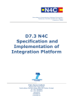
In addition, NetAnim also provides useful features such as tables to display meta-data of packets like the image below
and a way to visualize the trajectory of a mobile node
2.1.1 Methodology
The class ns3::AnimationInterface is responsible for the creation the trace XML file. AnimationInterface uses the
tracing infrastructure to track packet flows between nodes. AnimationInterface registers itself as a trace hook for tx and
rx events before the simulation begins. When a packet is scheduled for transmission or reception, the corresponding
tx and rx trace hooks in AnimationInterface are called. When the rx hooks are called, AnimationInterface will be
aware of the two endpoints between which a packet has flowed, and adds this information to the trace file, in XML
format along with the corresponding tx and rx timestamps. The XML format will be discussed in a later section. It is
important to note that AnimationInterface records a packet only if the rx trace hooks are called. Every tx event must
be matched by an rx event.
2.1.2 Downloading NetAnim
If NetAnim is not already available in the ns-3 package you downloaded, you can do the following:
Please ensure that you have installed mercurial. The latest version of NetAnim can be downloaded using mercurial
with the following command:
hg clone http://code.nsnam.org/netanim
5
ns-3 Model Library, Release ns-3.16
Figure 2.1: An example of packet animation on wired-links
6
Chapter 2. Animation
ns-3 Model Library, Release ns-3.16
Figure 2.2: An example of packet animation on wireless-links
2.1. NetAnim
7
ns-3 Model Library, Release ns-3.16
Figure 2.3: An example of tables for packet meta-data with protocol filters
8
Chapter 2. Animation
ns-3 Model Library, Release ns-3.16
Figure 2.4: An example of the trajectory of a mobile node
2.1. NetAnim
9
ns-3 Model Library, Release ns-3.16
2.1.3 Building NetAnim
Prerequisites
Qt4 (4.7 and over) is required to build NetAnim. This can be obtained using the following ways:
For Debian/Ubuntu Linux distributions:
apt-get install qt4-dev-tools
For Red Hat/Fedora based distribution:
yum install qt4
yum install qt4-devel
For Mac/OSX:
http://qt.nokia.com/downloads/
Build steps
To build NetAnim use the following commands:
cd netanim
make clean
qmake NetAnim.pro
make
(For MAC Users: qmake -spec macx-g++ NetAnim.pro)
Note: qmake could be “qmake-qt4” in some systems
This should create an executable named “NetAnim” in the same directory:
john@john-VirtualBox:~/netanim$ ls -l NetAnim
-rwxr-xr-x 1 john john 390395 2012-05-22 08:32 NetAnim
2.1.4 Usage
Using NetAnim is a two-step process
Step 1:Generate the animation XML trace file during simulation using “ns3::AnimationInterface” in the ns-3 code
base.
Step 2:Load the XML trace file generated in Step 1 with the offline Qt4-based animator named NetAnim.
Step 1: Generate XML animation trace file
The class “AnimationInterface” under “src/netanim” uses underlying ns-3 trace sources to construct a timestamped
ASCII file in XML format.
Examples are found under src/netanim/examples Example:
./waf -d debug configure --enable-examples
./waf --run "dumbbell-animation"
The above will create an XML file dumbbell-animation.xml
10
Chapter 2. Animation
ns-3 Model Library, Release ns-3.16
Mandatory
1. Ensure that your program’s wscript includes the “netanim” module. An example of such a wscript is at
src/netanim/examples/wscript.
2. Include the header [#include “ns3/netanim-module.h”] in your test program
3. Add the statement
AnimationInterface anim ("animation.xml");
where "animation.xml" is any arbitrary filename
[for versions before ns-3.13 you also have to use the line “anim.SetXMLOutput() to set the XML mode and also use
anim.StartAnimation();]
Optional
The following are optional but useful steps:
1.anim.SetMobilityPollInterval (Seconds (1));
AnimationInterface records the position of all nodes every 250 ms by default. The statement above sets the periodic
interval at which AnimationInterface records the position of all nodes. If the nodes are expected to move very little, it
is useful to set a high mobility poll interval to avoid large XML files.
2. anim.SetConstantPosition (Ptr< Node > n, double x, double y);
AnimationInterface requires that the position of all nodes be set. In ns-3 this is done by setting an associated MobilityModel. “SetConstantPosition” is a quick way to set the x-y coordinates of a node which is stationary.
3. anim.SetStartTime (Seconds(150)); and anim.SetStopTime (Seconds(150));
AnimationInterface can generate large XML files. The above statements restricts the window between which AnimationInterface does tracing. Restricting the window serves to focus only on relevant portions of the simulation and
creating manageably small XML files
4. AnimationInterface anim ("animation.xml", 50000);
Using the above constructor ensures that each animation XML trace file has only 50000 packets. For example, if
AnimationInterface captures 150000 packets, using the above constructor splits the capture into 3 files
animation.xml - containing the packet range 1-50000
animation.xml-1 - containing the packet range 50001-100000
animation.xml-2 - containing the packet range 100001-150000
5. anim.EnablePacketMetadata (true);
With the above statement, AnimationInterface records the meta-data of each packet in the xml trace file. Metadata
can be used by NetAnim to provide better statistics and filter, along with providing some brief information about the
packet such as TCP sequence number or source & destination IP address during packet animation.
CAUTION: Enabling this feature will result in larger XML trace files. Please do NOT enable this feature when using
Wimax links.
2.1. NetAnim
11
ns-3 Model Library, Release ns-3.16
Step 2: Loading the XML in NetAnim
1. Assuming NetAnim was built, use the command ”./NetAnim” to launch NetAnim. Please review the section
“Building NetAnim” if NetAnim is not available.
2. When NetAnim is opened, click on the File open button at the top-left corner, select the XML file generated
during Step 1.
3. Hit the green play button to begin animation.
Here is a video illustrating this http://www.youtube.com/watch?v=tz_hUuNwFDs
2.1.5 Essential settings of NetAnim
Persist combobox
Figure 2.5: The persist combobox
When packets are transmitted and received very quickly, they can be almost invisible. The persist time setting allows
the user to control the duration for which a packet should be visible on the animation canvas.
Update-interval slider
Figure 2.6: The update-interval slider
The update-interval slider controls the rate at which NetAnim refreshes the canvas screen. For instance, for the setting
above, NetAnim, updates the position of nodes and packets only once in 250 ms.
2.1.6 Parts of the XML
The XML trace files has the following main sections
1. Topology
• Nodes
• Links
2. packets (packets over wired-links)
3. wpackets (packets over wireless-links)
XML tags
Nodes are identified by their unique Node id. The XML begins with the “information” element describing the rest of
the elements
1. <anim> element
12
Chapter 2. Animation
ns-3 Model Library, Release ns-3.16
This is the XML root element. All other elements fall within this element. Attributes are:
lp = Logical Processor Id (Used for distributed simulations only)
2. <topology> element
This elements contains the Node and Link elements.It describes, the co-ordinates of the canvas used for animation.
Attributes are:
minX
minY
maxX
maxY
=
=
=
=
minimum
minimum
maximum
maximum
X
Y
X
Y
coordinate
coordinate
coordinate
coordinate
of
of
of
of
the
the
the
the
animation
animation
animation
animation
canvas
canvas
canvas
canvas
Example:
<topology minX = "-6.42025" minY = "-6.48444" maxX = "186.187" maxY = "188.049">
3. <node> element
This element describes each Node’s Id and X,Y co-ordinate (position). Attributes are:
id = Node Id
locX = X coordinate
locY = Y coordinate
Example:
<node id = "8" locX = "107.599" locY = "96.9366" />
4. <link> element
This element describes wired links between two nodes. Attributes are:
fromId = From Node Id (first node id)
toId
= To Node Id (second node id)
Example:
<link fromId="0" toId="1"/>
5. <p> element
This element describes a packet over wired links being transmitted at some node and received at another.
The reception details are described in its associated rx element Attributes are:
fId = Node Id transmitting the packet
fbTx = First bit transmit time of the packet
lbTx = Last bit transmit time of the packet
toId = Node Id receiving the packet
fbRx = First bit Reception Time of the packet
lbRx = Last bit Reception Time of the packet
Example:
<p fId="1" fbTx="1" lbTx="1.000067199" tId="0" fbRx="1.002" lbRx="1.002067199"/>
A packet over wired-links from Node 1 was received at Node 0. The first bit of the packet was transmitted at the 1st
second, the last bit was transmitted at the 1.000067199th second of the simulation Node 0 received the first bit of the
packet at the 1.002th second and the last bit of the packet at the 1.002067199th second of the simulation NOTE: A
packet with fromId == toId is a dummy packet used internally by the AnimationInterface. Please ignore this packet
7. <wp> element
2.1. NetAnim
13
ns-3 Model Library, Release ns-3.16
This element describes a packet over wireless links being transmitted at some node and received at another.
The reception details are described in its associated rx element. Attributes are:
fromId = Node Id transmitting the packet
fbTx = First bit transmit time of the packet
lbTx = Last bit transmit time of the packet
range = Range of the transmission
Example:
<wp fId = "20" fbTx = "0.003" lbTx = "0.003254" range = "59.68176982" tId="32" fbRx="0.003000198" lbR
A packet over wireless-links from Node 20 was received at Node 32. The first bit of the packet was transmitted at the
0.003th second, the last bit was transmitted at the 0.003254 second of the simulation Node 0 received the first bit of
the packet at the 0.003000198 second and the last bit of the packet at the 0.003254198 second of the simulation
2.1.7 Wiki
For detailed instructions on installing “NetAnim”, F.A.Qs and loading the XML trace file (mentioned earlier) using
NetAnim please refer: http://www.nsnam.org/wiki/index.php/NetAnim
14
Chapter 2. Animation
CHAPTER
THREE
ANTENNA MODULE
3.1 Design documentation
3.1.1 Overview
The Antenna module provides:
1. a new base class (AntennaModel) that provides an interface for the modeling of the radiation pattern of an
antenna;
2. a set of classes derived from this base class that each models the radiation pattern of different types of antennas.
3.1.2 AntennaModel
The AntennaModel uses the coordinate system adopted in [Balanis] and depicted in Figure Coordinate system of the
AntennaModel. This system is obtained by traslating the cartesian coordinate system used by the ns-3 MobilityModel
into the new origin o which is the location of the antenna, and then transforming the coordinates of every generic
point p of the space from cartesian coordinates (x, y, z) into spherical coordinates (r, θ, φ). The antenna model neglects the radial component r, and only considers the angle components (θ, φ). An antenna radiation pattern is then
expressed as a mathematical function g(θ, φ) −→ R that returns the gain (in dB) for each possible direction of transmission/reception. All angles are expressed in radians.
3.1.3 Provided models
In this section we describe the antenna radiation pattern models that are included within the antenna module.
IsotropicAntennaModel
This antenna radiation pattern model provides a unitary gain (0 dB) for all direction.
CosineAntennaModel
This is the cosine model described in [Chunjian]: the antenna gain is determined as:
φ − φ0
g(φ, θ) = cosn
2
15
ns-3 Model Library, Release ns-3.16
Figure 3.1: Coordinate system of the AntennaModel
where φ0 is the azimuthal orientation of the antenna (i.e., its direction of maximum gain) and the exponential
n=−
3
20 log10 cos φ3dB
4
determines the desired 3dB beamwidth φ3dB .
A major difference between the model of [Chunjian] and the one implemented in the class CosineAntennaModel is that
only the element factor (i.e., what described by the above formulas) is considered. In fact, [Chunjian] also considered
an additional antenna array factor. The reason why the latter is excluded is that we expect that the average user would
desire to specify a given beamwidth exactly, without adding an array factor at a latter stage which would in practice
alter the effective beamwidth of the resulting radiation pattern.
ParabolicAntennaModel
This model is based on the parabolic approximation of the main lobe radiation pattern. It is often used in the context
of cellular system to model the radiation pattern of a cell sector, see for instance [R4-092042a] and [Calcev]. The
antenna gain in dB is determined as:
!
2
φ − φ0
gdB (φ, θ) = − min 12
, Amax
φ3dB
where φ0 is the azimuthal orientation of the antenna (i.e., its direction of maximum gain), φ3dB is its 3 dB beamwidth,
and Amax is the maximum attenuation in dB of the antenna.
3.2 User Documentation
The antenna moduled can be used with all the wireless technologies and physical layer models that support it. Currently, this includes the physical layer models based on the SpectrumPhy. Please refer to the documentation of each of
these models for details.
16
Chapter 3. Antenna Module
ns-3 Model Library, Release ns-3.16
3.3 Testing Documentation
In this section we describe the test suites included with the antenna module that verify its correct functionality.
3.3.1 Angles
The unit test suite angles verifies that the Angles class is constructed properly by correct conversion from 3D
cartesian coordinates according to the available methods (construction from a single vector and from a pair of vectors).
For each method, several test cases are provided that compare the values (φ, θ) determied by the constructor to known
reference values. The test passes if for each case the values are equal to the reference up to a tolerance of 10−10 which
accounts for numerical errors.
3.3.2 DegreesToRadians
The unit test suite degrees-radians verifies that the methods DegreesToRadians and
RadiansToDegrees work properly by comparing with known reference values in a number of test cases.
Each test case passes if the comparison is equal up to a tolerance of 10−10 which accounts for numerical errors.
3.3.3 IsotropicAntennaModel
The unit test suite isotropic-antenna-model checks that the IsotropicAntennaModel class works properly, i.e., returns always a 0dB gain regardless of the direction.
3.3.4 CosineAntennaModel
The unit test suite cosine-antenna-model checks that the CosineAntennaModel class works properly.
Several test cases are provided that check for the antenna gain value calculated at different directions and for different
values of the orientation, the reference gain and the beamwidth. The reference gain is calculated by hand. Each test
case passes if the reference gain in dB is equal to the value returned by CosineAntennaModel within a tolerance
of 0.001, which accounts for the approximation done for the calculation of the reference values.
3.3.5 ParabolicAntennaModel
The unit test suite parabolic-antenna-model checks that the ParabolicAntennaModel class works properly. Several test cases are provided that check for the antenna gain value calculated at different directions and for
different values of the orientation, the maximum attenuation and the beamwidth. The reference gain is calculated by
hand. Each test case passes if the reference gain in dB is equal to the value returned by ParabolicAntennaModel
within a tolerance of 0.001, which accounts for the approximation done for the calculation of the reference values.
3.3. Testing Documentation
17
ns-3 Model Library, Release ns-3.16
18
Chapter 3. Antenna Module
CHAPTER
FOUR
AD HOC ON-DEMAND DISTANCE
VECTOR (AODV)
This model implements the base specification of the Ad Hoc On-Demand Distance Vector (AODV) protocol. The
implementation is based on [rfc3561].
The model was written by Elena Buchatskaia and Pavel Boyko of ITTP RAS, and is based on the ns-2 AODV model
developed by the CMU/MONARCH group and optimized and tuned by Samir Das and Mahesh Marina, University of
Cincinnati, and also on the AODV-UU implementation by Erik Nordström of Uppsala University.
4.1 Model Description
The source code for the AODV model lives in the directory src/aodv.
4.1.1 Design
Class ns3::aodv::RoutingProtocol implements all functionality of service packet exchange and inherits
from ns3::Ipv4RoutingProtocol. The base class defines two virtual functions for packet routing and forwarding. The first one, ns3::aodv::RouteOutput, is used for locally originated packets, and the second one,
ns3::aodv::RouteInput, is used for forwarding and/or delivering received packets.
Protocol operation depends on many adjustable parameters. Parameters for this functionality are attributes of
ns3::aodv::RoutingProtocol. Parameter default values are drawn from the RFC and allow the enabling/disabling protocol features, such as broadcasting HELLO messages, broadcasting data packets and so on.
AODV discovers routes on demand.
Therefore, the AODV model buffers all packets while
a route request packet (RREQ) is disseminated.
A packet queue is implemented in aodvrqueue.cc.
A smart pointer to the packet, ns3::Ipv4RoutingProtocol::ErrorCallback,
ns3::Ipv4RoutingProtocol::UnicastForwardCallback, and the IP header are stored in this
queue. The packet queue implements garbage collection of old packets and a queue size limit.
The routing table implementation supports garbage collection of old entries and state machine, defined in the standard.
It is implemented as a STL map container. The key is a destination IP address.
Some elements of protocol operation aren’t described in the RFC. These elements generally concern cooperation of
different OSI model layers. The model uses the following heuristics:
• This AODV implementation can detect the presence of unidirectional links and avoid them if necessary. If the
node the model receives an RREQ for is a neighbor, the cause may be a unidirectional link. This heuristic is
taken from AODV-UU implementation and can be disabled.
19
ns-3 Model Library, Release ns-3.16
• Protocol operation strongly depends on broken link detection mechanism. The model implements two such
heuristics. First, this implementation support HELLO messages. However HELLO messages are not a good
way to perform neighbor sensing in a wireless environment (at least not over 802.11). Therefore, one may experience bad performance when running over wireless. There are several reasons for this: 1) HELLO messages
are broadcasted. In 802.11, broadcasting is often done at a lower bit rate than unicasting, thus HELLO messages
can travel further than unicast data. 2) HELLO messages are small, thus less prone to bit errors than data transmissions, and 3) Broadcast transmissions are not guaranteed to be bidirectional, unlike unicast transmissions.
Second, we use layer 2 feedback when possible. Link are considered to be broken if frame transmission results
in a transmission failure for all retries. This mechanism is meant for active links and works faster than the first
method.
The layer 2 feedback implementation relies on the TxErrHeader trace source, currently supported in AdhocWifiMac
only.
4.1.2 Scope and Limitations
The model is for IPv4 only. The following optional protocol optimizations are not implemented:
1. Expanding ring search.
2. Local link repair.
3. RREP, RREQ and HELLO message extensions.
These techniques require direct access to IP header, which contradicts the assertion from the AODV RFC that AODV
works over UDP. This model uses UDP for simplicity, hindering the ability to implement certain protocol optimizations. The model doesn’t use low layer raw sockets because they are not portable.
4.1.3 Future Work
No announced plans.
20
Chapter 4. Ad Hoc On-Demand Distance Vector (AODV)
ns-3 Model Library, Release ns-3.16
4.1.4 References
4.2 Usage
4.2.1 Examples
4.2.2 Helpers
4.2.3 Attributes
4.2.4 Tracing
4.2.5 Logging
4.2.6 Caveats
4.3 Validation
4.3.1 Unit tests
4.3.2 Larger-scale performance tests
4.2. Usage
21
ns-3 Model Library, Release ns-3.16
22
Chapter 4. Ad Hoc On-Demand Distance Vector (AODV)
CHAPTER
FIVE
APPLICATIONS
Placeholder chapter
23
ns-3 Model Library, Release ns-3.16
24
Chapter 5. Applications
CHAPTER
SIX
BRIDGE NETDEVICE
Placeholder chapter
Some examples of the use of Bridge NetDevice can be found in examples/csma/ directory.
25
ns-3 Model Library, Release ns-3.16
26
Chapter 6. Bridge NetDevice
CHAPTER
SEVEN
BRITE INTEGRATION
This model implements an interface to BRITE, the Boston university Representative Internet Topology gEnerator 1 .
BRITE is a standard tool for generating realistic internet topologies. The ns-3 model, described herein, provides
a helper class to facilitate generating ns-3 specific topologies using BRITE configuration files. BRITE builds the
original graph which is stored as nodes and edges in the ns-3 BriteTopolgyHelper class. In the ns-3 integration of
BRITE, the generator generates a topology and then provides access to leaf nodes for each AS generated. ns-3 users
can than attach custom topologies to these leaf nodes either by creating them manually or using topology generators
provided in ns-3.
There are three major types of topologies available in BRITE: Router, AS, and Hierarchical which is a combination of
AS and Router. For the purposes of ns-3 simulation, the most useful are likely to be Router and Hierarchical. Router
level topologies be generated using either the Waxman model or the Barabasi-Albert model. Each model has different
parameters that effect topology creation. For flat router topologies, all nodes are considered to be in the same AS.
BRITE Hierarchical topologies contain two levels. The first is the AS level. This level can be also be created by
using either the Waxman model or the Barabasi-Albert model. Then for each node in the AS topology, a router
level topology is constructed. These router level topologies can again either use the Waxman model or the BarbasiAlbert model. BRITE interconnects these separate router topologies as specified by the AS level topology. Once the
hierarchical topology is constructed, it is flattened into a large router level topology.
Further information can be found in the BRITE user manual::
http://www.cs.bu.edu/brite/publications/usermanual.pdf
7.1 Model Description
The model relies on building an external BRITE library, and then building some ns-3 helpers that call out to the library.
The source code for the ns-3 helpers lives in the directory src/brite/helper.
7.1.1 Design
To generate the BRITE topology, ns-3 helpers call out to the external BRITE library, and using a standard BRITE
configuration file, the BRITE code builds a graph with nodes and edges according to this configuration file. Please see
the BRITE documenation or the example configuration files in src/brite/examples/conf_files to get a better grasp of
BRITE configuration options. The graph built by BRITE is returned to ns-3, and a ns-3 implementation of the graph
is built. Leaf nodes for each AS are available for the user to either attach custom topologies or install ns-3 applications
directly.
1 Alberto Medina, Anukool Lakhina, Ibrahim Matta, and John Byers. BRITE: An Approach to Universal Topology Generation. In Proceedings
of the International Workshop on Modeling, Analysis and Simulation of Computer and Telecommunications Systems- MASCOTS ‘01, Cincinnati,
Ohio, August 2001.
27
ns-3 Model Library, Release ns-3.16
7.1.2 References
7.2 Usage
The brite-generic-example can be referenced to see basic usage of the BRITE interface. In summary, the BriteTopologyHelper is used as the interface point by passing in a BRITE configuration file. Along with the configuration file a
BRITE formatted random seed file can also be passed in. If a seed file is not passed in, the helper will create a seed
file using ns-3’s UniformRandomVariable. Once the topology has been generated by BRITE, BuildBriteTopology()
is called to create the ns-3 representation. Next IP Address can be assigned to the topology using either AssignIpv4Addresses() or AssignIpv6Addresses(). It should be noted that each point-to-point link in the topology will
be treated as a new network therefore for IPV4 a /30 subnet should be used to avoid wasting a large amount of the
available address space.
Example BRITE configuration files can be found in /src/brite/examples/conf_files/. ASBarbasi and ASWaxman are
examples of AS only topologies. The RTBarabasi and RTWaxman files are examples of router only topologies. Finally
the TD_ASBarabasi_RTWaxman configuration file is an example of a Hierarchical topology that uses the BarabasiAlbert model for the AS level and the Waxman model for each of the router level topologies. Information on the
BRITE parameters used in these files can be found in the BRITE user manual.
7.2.1 Building BRITE Integration
The first step is to download and build the ns-3 specific BRITE repository::
$ hg clone http://code.nsnam.org/BRITE
$ cd BRITE
$ make
This will build BRITE and create a library, libbrite.so, within the BRITE directory.
Once BRITE has been built successfully, we proceed to configure ns-3 with BRITE support. Change to your ns-3
directory::
$ ./waf configure --with-brite=/your/path/to/brite/source --enable-examples
Make sure it says ‘enabled’ beside ‘BRITE Integration’. If it does not, then something has gone wrong. Either you
have forgotten to build BRITE first following the steps above, or ns-3 could not find your BRITE directory.
Next, build ns-3::
$ ./waf
7.2.2 Examples
For an example demonstrating BRITE integration run::
$ ./waf --run ’brite-generic-example’
By enabling the verbose parameter, the example will print out the node and edge information in a similar format
to standard BRITE output. There are many other command-line parameters including confFile, tracing, and nix,
described below:
confFile: A BRITE configuration file. Many different BRITE configuration file examples exist in
the src/brite/examples/conf_files directory, for example, RTBarabasi20.conf and RTWaxman.conf.
Please refer to the conf_files directory for more examples.
tracing: Enables ascii tracing.
28
Chapter 7. BRITE Integration
ns-3 Model Library, Release ns-3.16
nix: Enables nix-vector routing. Global routing is used by default.
The generic BRITE example also support visualization using pyviz, assuming python bindings in ns-3 are enabled::
$ ./waf --run brite-generic-example --vis
Simulations involving BRITE can also be used with MPI. The total number of MPI instances is passed to the BRITE
topology helper where a modulo divide is used to assign the nodes for each AS to a MPI instance. An example can be
found in src/brite/examples::
$ mpirun -np 2 ./waf --run brite-MPI-example
Please see the ns-3 MPI documentation for information on setting up MPI with ns-3.
7.2. Usage
29
ns-3 Model Library, Release ns-3.16
30
Chapter 7. BRITE Integration
CHAPTER
EIGHT
BUILDINGS MODULE
cd .. include:: replace.txt
8.1 Design documentation
8.1.1 Overview
The Buildings module provides:
1. a new class (Building) that models the presence of a building in a simulation scenario;
2. a new mobility model (BuildingsMobilityModel) that allows to specify the location, size and characteristics of buildings present in the simulated area, and allows the placement of nodes inside those buildings;
3. a container class with the definition of the most useful pathloss models and the correspondent variables called
BuildingsPropagationLossModel.
4. a new propagation model (HybridBuildingsPropagationLossModel) working with the mobility
model just introduced, that allows to model the phenomenon of indoor/outdoor propagation in the presence
of buildings.
5. a simplified model working only with Okumura Hata (OhBuildingsPropagationLossModel) considering the phenomenon of indoor/outdoor propagation in the presence of buildings.
The models have been designed with LTE in mind, though their implementation is in fact independent from any
LTE-specific code, and can be used with other ns-3 wireless technologies as well (e.g., wifi, wimax).
The HybridBuildingsPropagationLossModel pathloss model included is obtained through a combination
of several well known pathloss models in order to mimic different environmental scenarios such as urban, suburban
and open areas. Moreover, the model considers both outdoor and indoor indoor and outdoor communication has to be
included since HeNB might be installed either within building and either outside. In case of indoor communication,
the model has to consider also the type of building in outdoor <-> indoor communication according to some general
criteria such as the wall penetration losses of the common materials; moreover it includes some general configuration
for the internal walls in indoor communications.
The OhBuildingsPropagationLossModel pathloss model has been created for simplifying the previous one
removing the thresholds for switching from one model to other. For doing this it has been used only one propagation
model from the one available (i.e., the Okumura Hata). The presence of building is still considered in the model;
therefore all the considerations of above regarding the building type are still valid. The same consideration can be
done for what concern the environmental scenario and frequency since both of them are parameters of the model
considered.
31
ns-3 Model Library, Release ns-3.16
8.1.2 The Building class
The model includes a specific class called Building which contains a ns3 Box class for defining the dimension of
the building. In order to implements the characteristics of the pathloss models included, the Building class supports
the following attributes:
• building type:
– Residential (default value)
– Office
– Commercial
• external walls type
– Wood
– ConcreteWithWindows (default value)
– ConcreteWithoutWindows
– StoneBlocks
• number of floors (default value 1, which means only ground-floor)
• number of rooms in x-axis (default value 1)
• number of rooms in y-axis (default value 1)
The Building class is based on the following assumptions:
• a buildings is represented as a rectangular parallelepiped (i.e., a box)
• the walls are parallel to the x, y, and z axis
• a building is divided into a grid of rooms, identified by the following parameters:
– number of floors
– number of rooms along the x-axis
– number of rooms along the y-axis
• the z axis is the vertical axis, i.e., floor numbers increase for increasing z axis values
• the x and y room indices start from 1 and increase along the x and y axis respectively
• all rooms in a building have equal size
8.1.3 The BuildingsMobilityModel class
The BuildingsMobilityModel class, which inherits from the ns3 class MobilityModel, is in charge of
managing the standard mobility functionalities plus providing information about the position of a node with respect to
building. The information managed by BuildingsMobilityModel is:
• whether the node is indoor or outdoor
• if indoor:
– in which building the node is
– in which room the node is positioned (x, y and floor room indices)
32
Chapter 8. Buildings Module
ns-3 Model Library, Release ns-3.16
The class BuildingsMobilityModel is used by BuildingsPropagationLossModel class, which inherits
from the ns3 class PropagationLossModel and manages the pathloss computation of the single components and
their composition according to the nodes’ positions. Moreover, it implements also the shadowing, that is the loss due
to obstacles in the main path (i.e., vegetation, buildings, etc.).
8.1.4 ItuR1238PropagationLossModel
This class implements a building-dependent indoor propagation loss model based on the ITU P.1238 model, which
includes losses due to type of building (i.e., residential, office and commercial). The analytical expression is given in
the following.
Ltotal = 20 log f + N log d + Lf (n) − 28[dB]
where:

 28 residential
30 of f ice
N=
: power loss coefficient [dB]

22 commercial

residential
 4n
15 + 4(n − 1) of f ice
Lf =

6 + 3(n − 1)
commercial
n : number of floors between base station and mobile (n ≥ 1)
f : frequency [MHz]
d : distance (where d > 1) [m]
8.1.5 BuildingsPropagationLossModel
The BuildingsPropagationLossModel provides an additional set of building-dependent pathloss model elements that
are used to implement different pathloss logics. These pathloss model elements are described in the following subsections.
External Wall Loss (EWL)
This component models the penetration loss through walls for indoor to outdoor communications and vice-versa. The
values are taken from the [cost231] model.
• Wood ~ 4 dB
• Concrete with windows (not metallized) ~ 7 dB
• Concrete without windows ~ 15 dB (spans between 10 and 20 in COST231)
• Stone blocks ~ 12 dB
Internal Walls Loss (IWL)
This component models the penetration loss occurring in indoor-to-indoor communications within the same building. The total loss is calculated assuming that each single internal wall has a constant penetration loss Lsiw , and
approximating the number of walls that are penetrated with the manhattan distance (in number of rooms) between the
transmitter and the receiver. In detail, let x1 , y1 , x2 , y2 denote the room number along the x and y axis respectively
for user 1 and 2; the total loss LIW L is calculated as
LIW L = Lsiw (|x1 − x2 | + |y1 − y2 |)
8.1. Design documentation
33
ns-3 Model Library, Release ns-3.16
Height Gain Model (HG)
This component model the gain due to the fact that the transmitting device is on a floor above the ground. In the
literature [turkmani] this gain has been evaluated as about 2 dB per floor. This gain can be applied to all the indoor to
outdoor communications and vice-versa.
Shadowing Model
The shadowing is modeled according to a log-normal distribution with variable standard deviation as function of the
connection characteristics. In the implementation we considered three main possible scenarios which correspond to
three standard deviations (i.e., the mean is always 0), in detail:
2
• outdoor (m_shadowingSigmaOutdoor, defaul value of 7 dB) → XO ∼ N (µO , σO
).
• indoor (m_shadowingSigmaIndoor, defaul value of 10 dB) → XI ∼ N (µI , σI2 ).
2
• external walls penetration (m_shadowingSigmaExtWalls, default value 5 dB) → XW ∼ N (µW , σW
)
The simulator generates a shadowing value per each active link according to nodes’ position the first time the link
is used for transmitting. In case of transmissions from outdoor nodes to indoor ones, and vice-versa, the standard
deviation (σIO ) has to be calculated as the square root of the sum of the quadratic values of the standard deviatio in
case of outdoor nodes and the one for the external walls penetration. This is due to the fact that that the components
producing the shadowing are independent of each other; therefore, the variance of a distribution resulting from the
sum of two independent normal ones is the sum of the variances.
X ∼ N (µ, σ 2 ) and Y ∼ N (ν, τ 2 )
Z = X + Y ∼ Z(µ + ν, σ 2 + τ 2 )
q
2 + σ2
⇒ σIO = σO
W
8.1.6 Pathloss logics
In the following we describe the different pathloss logic that are implemented by inheriting from BuildingsPropagationLossModel.
HybridBuildingsPropagationLossModel
The HybridBuildingsPropagationLossModel pathloss model included is obtained through a combination
of several well known pathloss models in order to mimic different outdoor and indoor scenarios, as well as indoorto-outdoor and outdoor-to-indoor scenarios. In detail, the class HybridBuildingsPropagationLossModel
integrates the following pathloss models:
• OkumuraHataPropagationLossModel
Kun2600MhzPropagationLossModel)
(OH)
(at
frequencies
>
2.3
GHz
substituted
by
• ItuR1411LosPropagationLossModel and ItuR1411NlosOverRooftopPropagationLossModel (I1411)
• ItuR1238PropagationLossModel (I1238)
• the pathloss elements of the BuildingsPropagationLossModel (EWL, HG, IWL)
The following pseudo-code illustrates how the different pathloss model elements described above are integrated in
HybridBuildingsPropagationLossModel:
34
Chapter 8. Buildings Module
ns-3 Model Library, Release ns-3.16
if (txNode is outdoor)
then
if (rxNode is outdoor)
then
if (distance > 1 km)
then
if (rxNode or txNode is below the rooftop)
then
L = I1411
else
L = OH
else
L = I1411
else (rxNode is indoor)
if (distance > 1 km)
then
if (rxNode or txNode is below the rooftop)
L = I1411 + EWL + HG
else
L = OH + EWL + HG
else
L = I1411 + EWL + HG
else (txNode is indoor)
if (rxNode is indoor)
then
if (same building)
then
L = I1238 + IWL
else
L = I1411 + 2*EWL
else (rxNode is outdoor)
if (distance > 1 km)
then
if (rxNode or txNode is below the rooftop)
then
L = I1411 + EWL + HG
else
L = OH + EWL + HG
else
L = I1411 + EWL
We note that, for the case of communication between two nodes below rooftop level with distance is greater then 1
km, we still consider the I1411 model, since OH is specifically designed for macro cells and therefore for antennas
above the roof-top level.
For the ITU-R P.1411 model we consider both the LOS and NLoS versions. In particular, we considers the LoS
propagation for distances that are shorted than a tunable threshold (m_itu1411NlosThreshold). In case on
NLoS propagation, the over the roof-top model is taken in consideration for modeling both macro BS and SC. In case
on NLoS several parameters scenario dependent have been included, such as average street width, orientation, etc. The
values of such parameters have to be properly set according to the scenario implemented, the model does not calculate
natively their values. In case any values is provided, the standard ones are used, apart for the height of the mobile and
BS, which instead their integrity is tested directly in the code (i.e., they have to be greater then zero). In the following
we give the expressions of the components of the model.
We also note that the use of different propagation models (OH, I1411, I1238 with their variants) in HybridBuildingsPropagationLossModel can result in discontinuities of the pathloss with respect to distance. A proper tuning of
the attributes (especially the distance threshold attributes) can avoid these discontinuities. However, since the behavior
of each model depends on several other parameters (frequency, node heigth, etc), there is no default value of these
8.1. Design documentation
35
ns-3 Model Library, Release ns-3.16
thresholds that can avoid the discontinuities in all possible configurations. Hence, an appropriate tuning of these
parameters is left to the user.
OhBuildingsPropagationLossModel
The OhBuildingsPropagationLossModel class has been created as a simple means to solve the discontinuity
problems of HybridBuildingsPropagationLossModel without doing scenario-specific parameter tuning.
The solution is to use only one propagation loss model (i.e., Okumura Hata), while retaining the structure of the
pathloss logic for the calculation of other path loss components (such as wall penetration losses). The result is a model
that is free of discontinuities (except those due to walls), but that is less realistic overall for a generic scenario with
buildings and outdoor/indoor users, e.g., because Okumura Hata is not suitable neither for indoor communications nor
for outdoor communications below rooftop level.
In detail, the class OhBuildingsPropagationLossModel integrates the following pathloss models:
• OkumuraHataPropagationLossModel (OH)
• the pathloss elements of the BuildingsPropagationLossModel (EWL, HG, IWL)
The following pseudo-code illustrates how the different pathloss model elements described above are integrated in
OhBuildingsPropagationLossModel:
if (txNode is outdoor)
then
if (rxNode is outdoor)
then
L = OH
else (rxNode is indoor)
L = OH + EWL
else (txNode is indoor)
if (rxNode is indoor)
then
if (same building)
then
L = OH + IWL
else
L = OH + 2*EWL
else (rxNode is outdoor)
L = OH + EWL
We note that OhBuildingsPropagationLossModel is a significant simplification with respect to HybridBuildingsPropagationLossModel, due to the fact that OH is used always. While this gives a less accurate model in some scenarios
(especially below rooftop and indoor), it effectively avoids the issue of pathloss discontinuities that affects HybridBuildingsPropagationLossModel.
8.2 User Documentation
8.2.1 Main configurable parameters
The Building class has the following configurable parameters:
• building type: Residential, Office and Commercial.
• external walls type: Wood, ConcreteWithWindows, ConcreteWithoutWindows and StoneBlocks.
• building bounds: a Box class with the building bounds.
36
Chapter 8. Buildings Module
ns-3 Model Library, Release ns-3.16
• number of floors.
• number of rooms in x-axis and y-axis (rooms can be placed only in a grid way).
The BuildingMobilityLossModel parameter configurable with the ns3 attribute system is represented by the
bound (string Bounds) of the simulation area by providing a Box class with the area bounds. Moreover, by means of
its methos the following parameters can be configured:
• the number of floor the node is placed (default 0).
• the position in the rooms grid.
The BuildingPropagationLossModel class has the following configurable parameters configurable with the
attribute system:
• Frequency: reference frequency (default 2160 MHz), note that by setting the frequency the wavelength is set
accordingly automatically and viceversa).
• Lambda: the wavelength (0.139 meters, considering the above frequency).
• ShadowSigmaOutdoor: the standard deviation of the shadowing for outdoor nodes (defaul 7.0).
• ShadowSigmaIndoor: the standard deviation of the shadowing for indoor nodes (default 8.0).
• ShadowSigmaExtWalls: the standard deviation of the shadowing due to external walls penetration for
outdoor to indoor communications (default 5.0).
• RooftopLevel: the level of the rooftop of the building in meters (default 20 meters).
• Los2NlosThr: the value of distance of the switching point between line-of-sigth and non-line-of-sight propagation model in meters (default 200 meters).
• ITU1411DistanceThr: the value of distance of the switching point between short range (ITU 1211) communications and long range (Okumura Hata) in meters (default 200 meters).
• MinDistance: the minimum distance in meters between two nodes for evaluating the pathloss (considered
neglictible before this threshold) (default 0.5 meters).
• Environment: the environment scenario among Urban, SubUrban and OpenAreas (default Urban).
• CitySize: the dimension of the city among Small, Medium, Large (default Large).
In order to use the hybrid mode, the class to be used is the HybridBuildingMobilityLossModel, which allows
the selection of the proper pathloss model according to the pathloss logic presented in the design chapter. However,
this solution has the problem that the pathloss model switching points might present discontinuities due to the different
characteristics of the model. This implies that according to the specific scenario, the threshold used for switching have
to be properly tuned. The simple OhBuildingMobilityLossModel overcome this problem by using only the
Okumura Hata model and the wall penetration losses.
8.3 Testing Documentation
8.3.1 Overview
To test and validate the ns-3 Building Pathloss module, some test suites is provided which are integrated with the ns-3
test framework. To run them, you need to have configured the build of the simulator in this way:
./waf configure --enable-tests --enable-modules=buildings
./test.py
8.3. Testing Documentation
37
ns-3 Model Library, Release ns-3.16
The above will run not only the test suites belonging to the buildings module, but also those belonging to all the other
ns-3 modules on which the buildings module depends. See the ns-3 manual for generic information on the testing
framework.
You can get a more detailed report in HTML format in this way:
./test.py -w results.html
After the above command has run, you can view the detailed result for each test by opening the file results.html
with a web browser.
You can run each test suite separately using this command:
./test.py -s test-suite-name
For more details about test.py and the ns-3 testing framework, please refer to the ns-3 manual.
8.3.2 Description of the test suites
BuildingsHelper test
The test suite buildings-helper checks that the method BuildingsHelper::MakeAllInstancesConsistent
() works properly, i.e., that the BuildingsHelper is successful in locating if nodes are outdoor or indoor, and if indoor
that they are located in the correct building, room and floor. Several test cases are provided with different buildings
(having different size, position, rooms and floors) and different node positions. The test passes if each every node is
located correctly.
BuildingPositionAllocator test
The test suite building-position-allocator feature two test cases that check that respectively RandomRoomPositionAllocator and SameRoomPositionAllocator work properly. Each test cases involves a single 2x3x2
room building (total 12 rooms) at known coordinates and respectively 24 and 48 nodes. Both tests check that the
number of nodes allocated in each room is the expected one and that the position of the nodes is also correct.
Buildings Pathloss tests
The test suite buildings-pathloss-model provides different unit tests that compare the expected results of
the buildings pathloss module in specific scenarios with pre calculated values obtained offline with an Octave script
(test/reference/buildings-pathloss.m). The tests are considered passed if the two values are equal up to a tolerance of
0.1, which is deemed appropriate for the typical usage of pathloss values (which are in dB).
In the following we detailed the scenarios considered, their selection has been done for covering the wide set of
possible pathloss logic combinations. The pathloss logic results therefore implicitly tested.
Test #1 Okumura Hata
In this test we test the standard Okumura Hata model; therefore both eNB and UE are placed outside at a distance
of 2000 m. The frequency used is the E-UTRA band #5, which correspond to 869 MHz (see table 5.5-1 of 36.101).
The test includes also the validation of the areas extensions (i.e., urban, suburban and open-areas) and of the city size
(small, medium and large).
38
Chapter 8. Buildings Module
ns-3 Model Library, Release ns-3.16
Test #2 COST231 Model
This test is aimed at validating the COST231 model. The test is similar to the Okumura Hata one, except that the
frequency used is the EUTRA band #1 (2140 MHz) and that the test can be performed only for large and small cities
in urban scenarios due to model limitations.
Test #3 2.6 GHz model
This test validates the 2.6 GHz Kun model. The test is similar to Okumura Hata one except that the frequency is the
EUTRA band #7 (2620 MHz) and the test can be performed only in urban scenario.
Test #4 ITU1411 LoS model
This test is aimed at validating the ITU1411 model in case of line of sight within street canyons transmissions. In this
case the UE is placed at 100 meters far from the eNB, since the threshold for switching between LoS and NLoS is left
to default one (i.e., 200 m.).
Test #5 ITU1411 NLoS model
This test is aimed at validating the ITU1411 model in case of non line of sight over the rooftop transmissions. In this
case the UE is placed at 900 meters far from the eNB, in order to be above the threshold for switching between LoS
and NLoS is left to default one (i.e., 200 m.).
Test #6 ITUP1238 model
This test is aimed at validating the ITUP1238 model in case of indoor transmissions. In this case both the UE and the
eNB are placed in a residential building with walls made of concrete with windows. Ue is placed at the second floor
and distances 30 meters far from the eNB, which is placed at the first floor.
Test #7 Outdoor -> Indoor with Okumura Hata model
This test validates the outdoor to indoor transmissions for large distances. In this case the UE is placed in a residential
building with wall made of concrete with windows and distances 2000 meters from the outdoor eNB.
Test #8 Outdoor -> Indoor with ITU1411 model
This test validates the outdoor to indoor transmissions for short distances. In this case the UE is placed in a residential
building with walls made of concrete with windows and distances 100 meters from the outdoor eNB.
Test #9 Indoor -> Outdoor with ITU1411 model
This test validates the outdoor to indoor transmissions for very short distances. In this case the eNB is placed in the
second floor of a residential building with walls made of concrete with windows and distances 100 meters from the
outdoor UE (i.e., LoS communication). Therefore the height gain has to be included in the pathloss evaluation.
8.3. Testing Documentation
39
ns-3 Model Library, Release ns-3.16
Test #10 Indoor -> Outdoor with ITU1411 model
This test validates the outdoor to indoor transmissions for short distances. In this case the eNB is placed in the second
floor of a residential building with walls made of concrete with windows and distances 500 meters from the outdoor
UE (i.e., NLoS communication). Therefore the height gain has to be included in the pathloss evaluation.
Buildings Shadowing Test
The test suite buildings-shadowing-test is a unit test intended to verify the statistics distribution characteristics of the shadowing are the one expected. The shadowing is modeled according to a normal distribution with
mean µ = 0 and variable standard deviation σ, according to models commonly used in literature. The test generates 10,000 samples of shadowing by subtracting the deterministic component from the total loss returned by the
BuildingPathlossModel. The mean and variance of the shadowing samples are then used to verify whether the
99% confidence interval is respected by the sequence generated by the simulator.
8.4 References
40
Chapter 8. Buildings Module
CHAPTER
NINE
CLICK MODULAR ROUTER
INTEGRATION
Click is a software architecture for building configurable routers. By using different combinations of packet processing
units called elements, a Click router can be made to perform a specific kind of functionality. This flexibility provides
a good platform for testing and experimenting with different protocols.
9.1 Model Description
The source code for the Click model lives in the directory src/click.
9.1.1 Design
ns-3’s design is well suited for an integration with Click due to the following reasons:
• Packets in ns-3 are serialised/deserialised as they move up/down the stack. This allows ns-3 packets to be passed
to and from Click as they are.
• This also means that any kind of ns-3 traffic generator and transport should work easily on top of Click.
• By striving to implement click as an Ipv4RoutingProtocol instance, we can avoid significant changes to the LL
and MAC layer of the ns-3 code.
The design goal was to make the ns-3-click public API simple enough such that the user needs to merely add an
Ipv4ClickRouting instance to the node, and inform each Click node of the Click configuration file (.click file) that it is
to use.
This model implements the interface to the Click Modular Router and provides the Ipv4ClickRouting class to allow a
node to use Click for external routing. Unlike normal Ipv4RoutingProtocol sub types, Ipv4ClickRouting doesn’t use a
RouteInput() method, but instead, receives a packet on the appropriate interface and processes it accordingly. Note that
you need to have a routing table type element in your Click graph to use Click for external routing. This is needed by
the RouteOutput() function inherited from Ipv4RoutingProtocol. Furthermore, a Click based node uses a different kind
of L3 in the form of Ipv4L3ClickProtocol, which is a trimmed down version of Ipv4L3Protocol. Ipv4L3ClickProtocol
passes on packets passing through the stack to Ipv4ClickRouting for processing.
Developing a Simulator API to allow ns-3 to interact with Click
Much of the API is already well defined, which allows Click to probe for information from the simulator (like a Node’s
ID, an Interface ID and so forth). By retaining most of the methods, it should be possible to write new implementations
specific to ns-3 for the same functionality.
41
ns-3 Model Library, Release ns-3.16
Hence, for the Click integration with ns-3, a class named Ipv4ClickRouting will handle the interaction with Click. The
code for the same can be found in src/click/model/ipv4-click-routing.{cc,h}.
Packet hand off between ns-3 and Click
There are four kinds of packet hand-offs that can occur between ns-3 and Click.
• L4 to L3
• L3 to L4
• L3 to L2
• L2 to L3
To overcome this, we implement Ipv4L3ClickProtocol, a stripped down version of Ipv4L3Protocol.
Ipv4L3ClickProtocol passes packets to and from Ipv4ClickRouting appropriately to perform routing.
9.1.2 Scope and Limitations
• In its current state, the NS-3 Click Integration is limited to use only with L3, leaving NS-3 to handle L2. We are
currently working on adding Click MAC support as well. See the usage section to make sure that you design
your Click graphs accordingly.
• Furthermore, ns-3-click will work only with userlevel elements. The complete list of elements are available at
http://read.cs.ucla.edu/click/elements. Elements that have ‘all’, ‘userlevel’ or ‘ns’ mentioned beside them may
be used.
• As of now, the ns-3 interface to Click is Ipv4 only. We will be adding Ipv6 support in the future.
9.1.3 References
• Eddie Kohler, Robert Morris, Benjie Chen, John Jannotti, and M. Frans Kaashoek. The click modular router.
ACM Transactions on Computer Systems 18(3), August 2000, pages 263-297.
• Lalith Suresh P., and Ruben Merz. Ns-3-click: click modular router integration for ns-3. In Proc. of 3rd
International ICST Workshop on NS-3 (WNS3), Barcelona, Spain. March, 2011.
• Michael Neufeld, Ashish Jain, and Dirk Grunwald. Nsclick: bridging network simulation and deployment.
MSWiM ‘02: Proceedings of the 5th ACM international workshop on Modeling analysis and simulation of
wireless and mobile systems, 2002, Atlanta, Georgia, USA. http://doi.acm.org/10.1145/570758.570772
9.2 Usage
9.2.1 Building Click
The first step is to fetch (http://read.cs.ucla.edu/click/download) and build Click. At the top of your Click source
directory:
$: ./configure --enable-userlevel --disable-linuxmodule --enable-nsclick --enable-wifi
$: make
42
Chapter 9. Click Modular Router Integration
ns-3 Model Library, Release ns-3.16
The –enable-wifi flag may be skipped if you don’t intend on using Click with Wifi. * Note: You don’t need to do a
‘make install’.
Once Click has been built successfully, change into the ns-3 directory and configure ns-3 with Click Integration
support:
$: ./waf configure --enable-examples --enable-tests --with-nsclick=/path/to/click/source
Hint: If you have click installed one directory above ns-3 (such as in the ns-3-allinone directory), and the name of
the directory is ‘click’ (or a symbolic link to the directory is named ‘click’), then the –with-nsclick specifier is not
necessary; the ns-3 build system will successfully find the directory.
If it says ‘enabled’ beside ‘NS-3 Click Integration Support’, then you’re good to go. Note: If running modular ns-3,
the minimum set of modules required to run all ns-3-click examples is wifi, csma and config-store.
Next, try running one of the examples:
$: ./waf --run nsclick-simple-lan
You may then view the resulting .pcap traces, which are named nsclick-simple-lan-0-0.pcap and nsclick-simple-lan-01.pcap.
9.2.2 Click Graph Instructions
The following should be kept in mind when making your Click graph:
• Only userlevel elements can be used.
• You will need to replace FromDevice and ToDevice elements with FromSimDevice and ToSimDevice elements.
• Packets to the kernel are sent up using ToSimDevice(tap0,IP).
• For any node, the device which sends/receives packets to/from the kernel, is named ‘tap0’. The remaining
interfaces should be named eth0, eth1 and so forth (even if you’re using wifi). Please note that the device
numbering should begin from 0. In future, this will be made flexible so that users can name devices in their
Click file as they wish.
• A routing table element is a mandatory. The OUTports of the routing table element should correspond to the
interface number of the device through which the packet will ultimately be sent out. Violating this rule will lead
to really weird packet traces. This routing table element’s name should then be passed to the Ipv4ClickRouting
protocol object as a simulation parameter. See the Click examples for details.
• The current implementation leaves Click with mainly L3 functionality, with ns-3 handling L2. We will soon
begin working to support the use of MAC protocols on Click as well. This means that as of now, Click’s Wifi
specific elements cannot be used with ns-3.
9.2.3 Debugging Packet Flows from Click
From any point within a Click graph, you may use the Print (http://read.cs.ucla.edu/click/elements/print) element and
its variants for pretty printing of packet contents. Furthermore, you may generate pcap traces of packets flowing
through a Click graph by using the ToDump (http://read.cs.ucla.edu/click/elements/todump) element as well. For
instance:
myarpquerier
-> Print(fromarpquery,64)
-> ToDump(out_arpquery,PER_NODE 1)
-> ethout;
9.2. Usage
43
ns-3 Model Library, Release ns-3.16
and ...will print the contents of packets that flow out of the ArpQuerier, then generate a pcap trace file which will have
a suffix ‘out_arpquery’, for each node using the Click file, before pushing packets onto ‘ethout’.
9.2.4 Helper
To have a node run Click, the easiest way would be to use the ClickInternetStackHelper class in your simulation script.
For instance:
ClickInternetStackHelper click;
click.SetClickFile (myNodeContainer, "nsclick-simple-lan.click");
click.SetRoutingTableElement (myNodeContainer, "u/rt");
click.Install (myNodeContainer);
The
example
scripts
inside
src/click/examples/
demonstrate
the
use
of
based
nodes
in
different
scenarios.
The
helper
source
can
be
found
src/click/helper/click-internet-stack-helper.{h,cc}
Click
inside
9.2.5 Examples
The following examples have been written, which can be found in src/click/examples/:
• nsclick-simple-lan.cc and nsclick-raw-wlan.cc: A Click based node communicating with a normal ns-3 node
without Click, using Csma and Wifi respectively. It also demonstrates the use of TCP on top of Click, something
which the original nsclick implementation for NS-2 couldn’t achieve.
• nsclick-udp-client-server-csma.cc and nsclick-udp-client-server-wifi.cc: A 3 node LAN (Csma and Wifi respectively) wherein 2 Click based nodes run a UDP client, that sends packets to a third Click based node running a
UDP server.
• nsclick-routing.cc: One Click based node communicates to another via a third node that acts as an IP router
(using the IP router Click configuration). This demonstrates routing using Click.
Scripts are available within <click-dir>/conf/ that allow you to generate Click files for some common scenarios. The IP Router used in nsclick-routing.cc was generated from the make-ip-conf.pl file and slightly
adapted to work with ns-3-click.
9.3 Validation
This model has been tested as follows:
• Unit tests have been written to verify the internals of Ipv4ClickRouting.
This can be found in
src/click/ipv4-click-routing-test.cc.
These tests verify whether the methods inside
Ipv4ClickRouting which deal with Device name to ID, IP Address from device name and Mac Address from
device name bindings work as expected.
• The examples have been used to test Click with actual simulation scenarios. These can be found in
src/click/examples/. These tests cover the following: the use of different kinds of transports on top
of Click, TCP/UDP, whether Click nodes can communicate with non-Click based nodes, whether Click nodes
can communicate with each other, using Click to route packets using static routing.
• Click has been tested with Csma, Wifi and Point-to-Point devices. Usage instructions are available in the preceding section.
44
Chapter 9. Click Modular Router Integration
CHAPTER
TEN
CSMA NETDEVICE
This is the introduction to CSMA NetDevice chapter, to complement the Csma model doxygen.
10.1 Overview of the CSMA model
The ns-3 CSMA device models a simple bus network in the spirit of Ethernet. Although it does not model any real
physical network you could ever build or buy, it does provide some very useful functionality.
Typically when one thinks of a bus network Ethernet or IEEE 802.3 comes to mind. Ethernet uses CSMA/CD (Carrier Sense Multiple Access with Collision Detection with exponentially increasing backoff to contend for the shared
transmission medium. The ns-3 CSMA device models only a portion of this process, using the nature of the globally
available channel to provide instantaneous (faster than light) carrier sense and priority-based collision “avoidance.”
Collisions in the sense of Ethernet never happen and so the ns-3 CSMA device does not model collision detection, nor
will any transmission in progress be “jammed.”
10.1.1 CSMA Layer Model
There are a number of conventions in use for describing layered communications architectures in the literature and in
textbooks. The most common layering model is the ISO seven layer reference model. In this view the CsmaNetDevice
and CsmaChannel pair occupies the lowest two layers – at the physical (layer one), and data link (layer two) positions.
Another important reference model is that specified by RFC 1122, “Requirements for Internet Hosts – Communication
Layers.” In this view the CsmaNetDevice and CsmaChannel pair occupies the lowest layer – the link layer. There is
also a seemingly endless litany of alternative descriptions found in textbooks and in the literature. We adopt the naming
conventions used in the IEEE 802 standards which speak of LLC, MAC, MII and PHY layering. These acronyms are
defined as:
• LLC: Logical Link Control;
• MAC: Media Access Control;
• MII: Media Independent Interface;
• PHY: Physical Layer.
In this case the LLC and MAC are sublayers of the OSI data link layer and the MII and PHY are sublayers of the OSI
physical layer.
The “top” of the CSMA device defines the transition from the network layer to the data link layer. This transition is
performed by higher layers by calling either CsmaNetDevice::Send or CsmaNetDevice::SendFrom.
In contrast to the IEEE 802.3 standards, there is no precisely specified PHY in the CSMA model in the sense of wire
types, signals or pinouts. The “bottom” interface of the CsmaNetDevice can be thought of as as a kind of Media
45
ns-3 Model Library, Release ns-3.16
Independent Interface (MII) as seen in the “Fast Ethernet” (IEEE 802.3u) specifications. This MII interface fits into a
corresponding media independent interface on the CsmaChannel. You will not find the equivalent of a 10BASE-T or
a 1000BASE-LX PHY.
The CsmaNetDevice calls the CsmaChannel through a media independent interface. There is a method defined to tell
the channel when to start “wiggling the wires” using the method CsmaChannel::TransmitStart, and a method to tell
the channel when the transmission process is done and the channel should begin propagating the last bit across the
“wire”: CsmaChannel::TransmitEnd.
When the TransmitEnd method is executed, the channel will model a single uniform signal propagation delay in the
medium and deliver copes of the packet to each of the devices attached to the packet via the CsmaNetDevice::Receive
method.
There is a “pin” in the device media independent interface corresponding to “COL” (collision). The state of the channel
may be sensed by calling CsmaChannel::GetState. Each device will look at this “pin” before starting a send and will
perform appropriate backoff operations if required.
Properly received packets are forwarded up to higher levels from the CsmaNetDevice via a callback mechanism.
The callback function is initialized by the higher layer (when the net device is attached) using CsmaNetDevice::SetReceiveCallback and is invoked upon “proper” reception of a packet by the net device in order to forward
the packet up the protocol stack.
10.2 CSMA Channel Model
The class CsmaChannel models the actual transmission medium. There is no fixed limit for the number of devices
connected to the channel. The CsmaChannel models a data rate and a speed-of-light delay which can be accessed via
the attributes “DataRate” and “Delay” respectively. The data rate provided to the channel is used to set the data rates
used by the transmitter sections of the CSMA devices connected to the channel. There is no way to independently set
data rates in the devices. Since the data rate is only used to calculate a delay time, there is no limitation (other than
by the data type holding the value) on the speed at which CSMA channels and devices can operate; and no restriction
based on any kind of PHY characteristics.
The CsmaChannel has three states, IDLE, TRANSMITTING and PROPAGATING. These three states are “seen” instantaneously by all devices on the channel. By this we mean that if one device begins or ends a simulated transmission,
all devices on the channel are immediately aware of the change in state. There is no time during which one device may
see an IDLE channel while another device physically further away in the collision domain may have begun transmitting with the associated signals not propagated down the channel to other devices. Thus there is no need for collision
detection in the CsmaChannel model and it is not implemented in any way.
We do, as the name indicates, have a Carrier Sense aspect to the model. Since the simulator is single threaded, access
to the common channel will be serialized by the simulator. This provides a deterministic mechanism for contending
for the channel. The channel is allocated (transitioned from state IDLE to state TRANSMITTING) on a first-come
first-served basis. The channel always goes through a three state process::
IDLE -> TRANSMITTING -> PROPAGATING -> IDLE
The TRANSMITTING state models the time during which the source net device is actually wiggling the signals on the
wire. The PROPAGATING state models the time after the last bit was sent, when the signal is propagating down the
wire to the “far end.”
The transition to the TRANSMITTING state is driven by a call to CsmaChannel::TransmitStart which is called by
the net device that transmits the packet. It is the responsibility of that device to end the transmission with a call to
CsmaChannel::TransmitEnd at the appropriate simulation time that reflects the time elapsed to put all of the packet
bits on the wire. When TransmitEnd is called, the channel schedules an event corresponding to a single speed-oflight delay. This delay applies to all net devices on the channel identically. You can think of a symmetrical hub in
which the packet bits propagate to a central location and then back out equal length cables to the other devices on the
46
Chapter 10. CSMA NetDevice
ns-3 Model Library, Release ns-3.16
channel. The single “speed of light” delay then corresponds to the time it takes for: 1) a signal to propagate from one
CsmaNetDevice through its cable to the hub; plus 2) the time it takes for the hub to forward the packet out a port; plus
3) the time it takes for the signal in question to propagate to the destination net device.
The CsmaChannel models a broadcast medium so the packet is delivered to all of the devices on the channel (including
the source) at the end of the propagation time. It is the responsibility of the sending device to determine whether or
not it receives a packet broadcast over the channel.
The CsmaChannel provides following Attributes:
• DataRate: The bitrate for packet transmission on connected devices;
• Delay: The speed of light transmission delay for the channel.
10.3 CSMA Net Device Model
The CSMA network device appears somewhat like an Ethernet device. The CsmaNetDevice provides following Attributes:
• Address: The Mac48Address of the device;
• SendEnable: Enable packet transmission if true;
• ReceiveEnable: Enable packet reception if true;
• EncapsulationMode: Type of link layer encapsulation to use;
• RxErrorModel: The receive error model;
• TxQueue: The transmit queue used by the device;
• InterframeGap: The optional time to wait between “frames”;
• Rx: A trace source for received packets;
• Drop: A trace source for dropped packets.
The CsmaNetDevice supports the assignment of a “receive error model.” This is an ErrorModel object that is used to
simulate data corruption on the link.
Packets sent over the CsmaNetDevice are always routed through the transmit queue to provide a trace hook for packets
sent out over the network. This transmit queue can be set (via attribute) to model different queuing strategies.
Also configurable by attribute is the encapsulation method used by the device. Every packet gets an EthernetHeader
that includes the destination and source MAC addresses, and a length/type field. Every packet also gets an EthernetTrailer which includes the FCS. Data in the packet may be encapsulated in different ways.
By default, or by setting the “EncapsulationMode” attribute to “Dix”, the encapsulation is according to the DEC,
Intel, Xerox standard. This is sometimes called EthernetII framing and is the familiar destination MAC, source MAC,
EtherType, Data, CRC format.
If the “EncapsulationMode” attribute is set to “Llc”, the encapsulation is by LLC SNAP. In this case, a SNAP header
is added that contains the EtherType (IP or ARP).
The other implemented encapsulation modes are IP_ARP (set “EncapsulationMode” to “IpArp”) in which the length
type of the Ethernet header receives the protocol number of the packet; or ETHERNET_V1 (set “EncapsulationMode”
to “EthernetV1”) in which the length type of the Ethernet header receives the length of the packet. A “Raw” encapsulation mode is defined but not implemented – use of the RAW mode results in an assertion.
Note that all net devices on a channel must be set to the same encapsulation mode for correct results. The encapsulation
mode is not sensed at the receiver.
10.3. CSMA Net Device Model
47
ns-3 Model Library, Release ns-3.16
The CsmaNetDevice implements a random exponential backoff algorithm that is executed if the channel is determined
to be busy (TRANSMITTING or PPROPAGATING) when the device wants to start propagating. This results in a
random delay of up to pow (2, retries) - 1 microseconds before a retry is attempted. The default maximum number of
retries is 1000.
10.4 Using the CsmaNetDevice
The CSMA net devices and channels are typically created and configured using the associated CsmaHelper object.
The various ns-3 device helpers generally work in a similar way, and their use is seen in many of our example programs.
The conceptual model of interest is that of a bare computer “husk” into which you plug net devices. The bare computers
are created using a NodeContainer helper. You just ask this helper to create as many computers (we call them
Nodes) as you need on your network::
NodeContainer csmaNodes;
csmaNodes.Create (nCsmaNodes);
Once you have your nodes, you need to instantiate a CsmaHelper and set any attributes you may want to change.:
CsmaHelper csma;
csma.SetChannelAttribute ("DataRate", StringValue ("100Mbps"));
csma.SetChannelAttribute ("Delay", TimeValue (NanoSeconds (6560)));
csma.SetDeviceAttribute ("EncapsulationMode", StringValue ("Dix"));
csma.SetDeviceAttribute ("FrameSize", UintegerValue (2000));
Once the attributes are set, all that remains is to create the devices and install them on the required nodes, and to
connect the devices together using a CSMA channel. When we create the net devices, we add them to a container to
allow you to use them in the future. This all takes just one line of code.:
NetDeviceContainer csmaDevices = csma.Install (csmaNodes);
We recommend thinking carefully about changing these Attributes, since it can result in behavior that surprises users.
We allow this because we believe flexibility is important. As an example of a possibly surprising effect of changing
Attributes, consider the following:
The Mtu Attribute indicates the Maximum Transmission Unit to the device. This is the size of the largest Protocol
Data Unit (PDU) that the device can send. This Attribute defaults to 1500 bytes and corresponds to a number found
in RFC 894, “A Standard for the Transmission of IP Datagrams over Ethernet Networks.” The number is actually
derived from the maximum packet size for 10Base5 (full-spec Ethernet) networks – 1518 bytes. If you subtract DIX
encapsulation overhead for Ethernet packets (18 bytes) you will end up with a maximum possible data size (MTU)
of 1500 bytes. One can also find that the MTU for IEEE 802.3 networks is 1492 bytes. This is because LLC/SNAP
encapsulation adds an extra eight bytes of overhead to the packet. In both cases, the underlying network hardware is
limited to 1518 bytes, but the MTU is different because the encapsulation is different.
If one leaves the Mtu Attribute at 1500 bytes and changes the encapsulation mode Attribute to Llc, the result will be a
network that encapsulates 1500 byte PDUs with LLC/SNAP framing resulting in packets of 1526 bytes. This would
be illegal in many networks, but we allow you do do this. This results in a simulation that quite subtly does not reflect
what you might be expecting since a real device would balk at sending a 1526 byte packet.
There also exist jumbo frames (1500 < MTU <= 9000 bytes) and super-jumbo (MTU > 9000 bytes) frames that
are not officially sanctioned by IEEE but are available in some high-speed (Gigabit) networks and NICs. In the
CSMA model, one could leave the encapsulation mode set to Dix, and set the Mtu to 64000 bytes – even though an
associated CsmaChannel DataRate was left at 10 megabits per second (certainly not Gigabit Ethernet). This would
essentially model an Ethernet switch made out of vampire-tapped 1980s-style 10Base5 networks that support superjumbo datagrams, which is certainly not something that was ever made, nor is likely to ever be made; however it is
quite easy for you to configure.
48
Chapter 10. CSMA NetDevice
ns-3 Model Library, Release ns-3.16
Be careful about assumptions regarding what CSMA is actually modelling and how configuration (Attributes) may
allow you to swerve considerably away from reality.
10.5 CSMA Tracing
Like all ns-3 devices, the CSMA Model provides a number of trace sources. These trace sources can be hooked using
your own custom trace code, or you can use our helper functions to arrange for tracing to be enabled on devices you
specify.
10.5.1 Upper-Level (MAC) Hooks
From the point of view of tracing in the net device, there are several interesting points to insert trace hooks. A convention inherited from other simulators is that packets destined for transmission onto attached networks pass through
a single “transmit queue” in the net device. We provide trace hooks at this point in packet flow, which corresponds
(abstractly) only to a transition from the network to data link layer, and call them collectively the device MAC hooks.
When a packet is sent to the CSMA net device for transmission it always passes through the transmit queue. The
transmit queue in the CsmaNetDevice inherits from Queue, and therefore inherits three trace sources:
• An Enqueue operation source (see Queue::m_traceEnqueue);
• A Dequeue operation source (see Queue::m_traceDequeue);
• A Drop operation source (see Queue::m_traceDrop).
The upper-level (MAC) trace hooks for the CsmaNetDevice are, in fact, exactly these three trace sources on the single
transmit queue of the device.
The m_traceEnqueue event is triggered when a packet is placed on the transmit queue. This happens at the time that
CsmaNetDevice::Send or CsmaNetDevice::SendFrom is called by a higher layer to queue a packet for transmission.
The m_traceDequeue event is triggered when a packet is removed from the transmit queue. Dequeues from the transmit queue can happen in three situations: 1) If the underlying channel is idle when the CsmaNetDevice::Send or
CsmaNetDevice::SendFrom is called, a packet is dequeued from the transmit queue and immediately transmitted; 2)
If the underlying channel is idle, a packet may be dequeued and immediately transmitted in an internal TransmitCompleteEvent that functions much like a transmit complete interrupt service routine; or 3) from the random exponential
backoff handler if a timeout is detected.
Case (3) implies that a packet is dequeued from the transmit queue if it is unable to be transmitted according to the
backoff rules. It is important to understand that this will appear as a Dequeued packet and it is easy to incorrectly
assume that the packet was transmitted since it passed through the transmit queue. In fact, a packet is actually dropped
by the net device in this case. The reason for this behavior is due to the definition of the Queue Drop event. The
m_traceDrop event is, by definition, fired when a packet cannot be enqueued on the transmit queue because it is full.
This event only fires if the queue is full and we do not overload this event to indicate that the CsmaChannel is “full.”
10.5.2 Lower-Level (PHY) Hooks
Similar to the upper level trace hooks, there are trace hooks available at the lower levels of the net device. We call
these the PHY hooks. These events fire from the device methods that talk directly to the CsmaChannel.
The trace source m_dropTrace is called to indicate a packet that is dropped by the device. This happens in two cases:
First, if the receive side of the net device is not enabled (see CsmaNetDevice::m_receiveEnable and the associated
attribute “ReceiveEnable”).
The m_dropTrace is also used to indicate that a packet was discarded as corrupt if a receive error model is used (see
CsmaNetDevice::m_receiveErrorModel and the associated attribute “ReceiveErrorModel”).
10.5. CSMA Tracing
49
ns-3 Model Library, Release ns-3.16
The other low-level trace source fires on reception of an accepted packet (see CsmaNetDevice::m_rxTrace). A packet
is accepted if it is destined for the broadcast address, a multicast address, or to the MAC address assigned to the net
device.
10.6 Summary
The ns3 CSMA model is a simplistic model of an Ethernet-like network. It supports a Carrier-Sense function and
allows for Multiple Access to a shared medium. It is not physical in the sense that the state of the medium is instantaneously shared among all devices. This means that there is no collision detection required in this model and none
is implemented. There will never be a “jam” of a packet already on the medium. Access to the shared channel is on
a first-come first-served basis as determined by the simulator scheduler. If the channel is determined to be busy by
looking at the global state, a random exponential backoff is performed and a retry is attempted.
Ns-3 Attributes provide a mechanism for setting various parameters in the device and channel such as addresses,
encapsulation modes and error model selection. Trace hooks are provided in the usual manner with a set of upper level
hooks corresponding to a transmit queue and used in ASCII tracing; and also a set of lower level hooks used in pcap
tracing.
Although the ns-3 CsmaChannel and CsmaNetDevice does not model any kind of network you could build or buy, it
does provide us with some useful functionality. You should, however, understand that it is explicitly not Ethernet or
any flavor of IEEE 802.3 but an interesting subset.
50
Chapter 10. CSMA NetDevice
CHAPTER
ELEVEN
DSDV ROUTING
Destination-Sequenced Distance Vector (DSDV) routing protocol is a pro-active, table-driven routing protocol for
MANETs developed by Charles E. Perkins and Pravin Bhagwat in 1994. It uses the hop count as metric in route
selection.
This model was developed by the ResiliNets research group at the University of Kansas. A paper on this model exists
at this URL.
11.1 DSDV Routing Overview
DSDV Routing Table: Every node will maintain a table listing all the other nodes it has known either directly or
through some neighbors. Every node has a single entry in the routing table. The entry will have information about
the node’s IP address, last known sequence number and the hop count to reach that node. Along with these details the
table also keeps track of the nexthop neighbor to reach the destination node, the timestamp of the last update received
for that node.
The DSDV update message consists of three fields, Destination Address, Sequence Number and Hop Count.
Each node uses 2 mechanisms to send out the DSDV updates. They are,
1. Periodic Updates Periodic updates are sent out after every m_periodicUpdateInterval(default:15s). In this update the node broadcasts out its entire routing table.
2. Trigger Updates Trigger Updates are small updates in-between the periodic updates. These updates are sent
out whenever a node receives a DSDV packet that caused a change in its routing table. The original paper
did not clearly mention when for what change in the table should a DSDV update be sent out. The current
implemntation sends out an update irrespective of the change in the routing table.
The updates are accepted based on the metric for a particular node. The first factor determinig the acceptance of an
update is the sequence number. It has to accept the update if the sequence number of the update message is higher
irrespective of the metric. If the update with same sequence number is received, then the update with least metric
(hopCount) is given precedence.
In highly mobile scenarios, there is a high chance of route fluctuations, thus we have the concept of weighted settling
time where an update with change in metric will not be advertised to neighbors. The node waits for the settling time
to make sure that it did not receive the update from its old neighbor before sending out that update.
The current implementation covers all the above features of DSDV. The current implementation also has a request
queue to buffer packets that have no routes to destination. The default is set to buffer up to 5 packets per destination.
51
ns-3 Model Library, Release ns-3.16
11.2 References
Link to the Paper: http://portal.acm.org/citation.cfm?doid=190314.190336
52
Chapter 11. DSDV Routing
CHAPTER
TWELVE
DSR ROUTING
Dynamic Source Routing (DSR) protocol is a reactive routing protocol designed specifically for use in multi-hop
wireless ad hoc networks of mobile nodes.
This model was developed by the ResiliNets research group at the University of Kansas.
12.1 DSR Routing Overview
This model implements the base specification of the Dynamic Source Routing (DSR) protocol. Implementation is
based on RFC4728.
• Class dsr::DsrRouting implements all functionality of service packet exchange and inherits
IpL4Protocol.
• Class dsr::DsrOptions implements functionality of packet processing and talks to DsrRouting to
send/receive packets
• Class dsr::DsrFsHeader defines the fixed-size header and identifies the up-layer protocol
• Class dsr::DsrOptionHeader takes care of different dsr options and processes different header according to the specification from the RFC
• Class dsr::DsrSendBuffer is a buffer to save data packets and route error packets when there is no
route to forward the packets
• Class dsr::DsrMaintainBuffer is a buffer to save data packets for next-hop notification when the data
packet has already been sent out of send buffer
• Class dsr::RouteCache is the essential part to save routes found for data packets. DSR responds to
several routes for a single destination
• Class dsr::RreqTable implements the functions to avoid duplicate route requests and control route request rate for a single destination
Protocol operation depends on many adjustable parameters. We support parameters, with their default values, from
RFC and parameters that enable/disable protocol features or tune for specific simulation scenarios, such as the max
size of the send buffer and its timeout value. The full parameter list is found in the dsr-routing.cc file.
DSR discovers routes on-demand. Therefore, our DSR model buffers all packets, while a route request packet (RREQ)
is disseminated. We implement a packet buffer in dsr-rsendbuff.cc. The packet queue implements garbage collection
of old packets and a queue size limit. When the packet is sent out from the send buffer, it will be queued in maintenance
buffer for next hop acknowledgment.
The Route Cache implementation support garbage collection of old entries and state machine, as defined in the standard. It implements as a STL map container. The key is the destination IP address.
53
ns-3 Model Library, Release ns-3.16
Protocol operation strongly depends on broken link detection mechanism. We implement the three heuristics recommended.
First, we use layer 2 feedback when possible. A link is considered to be broken if frame transmission results in a
transmission failure for all retries. This mechanism is meant for active links and works much faster than in its absence.
Layer 2 feedback implementation relies on TxErrHeader trace source, currently it is supported in AdhocWifiMac only.
Second, passive acknowledgment should be used whenever possible. The node turns on “promiscuous” receive mode,
in which it can receive packets not destined for itself, and when the node assures the delivery of that data packet to its
destination, it cancels the passive acknowledgment timer.
Last, we use a network layer acknowledge scheme to notify the receipt of a packet. Route request packet will not be
acknowledged or retransmitted.
The following optional protocol optimizations aren’t implemented:
• Flow state
• First Hop External (F), Last Hop External (L) flags
• Handling unknown DSR options
• Two types of error headers:
1. flow state not supported option
2. unsupported option (not going to happen in simulation)
DSR operates with direct access to IP header, and operates between network and transport layer.
12.1.1 Implementation changes
• The DsrFsHeader has added 3 fields: message type, source id, destination id, and these changes only for postprocessing
– message type is used to identify the data packet from control packet
– source id is used to identify the real source of the data packet since we have to deliver the packet hop-byhop and the ipv4header is not carrying the real source and destination ip address as needed
– destination id is for same reason of above
• Route Reply header is not word-aligned in DSR rfc, change it to word-aligned in implementation
• DSR works as a shim header between transport and network protocol, it needs its own forwarding mechanism,
we are changing the packet transmission to hop-by-hop delivery, so we added two fields in dsr fixed header to
notify packet delivery
# message type to notify the type of this packet: data packet or control one # source id to identify the real source
address of this packet # destination id to identify the real destination
12.1.2 Current Route Cache implementation
This implementation used “path cache”, which is simple to implement and ensures loop-free paths:
• the path cache has automatic expire policy
• the cache saves multiple route entries for a certain destination and sort the entries based on hop counts
• the MaxEntriesEachDst can be tuned to change the maximum entries saved for a single destination
• when adding mulitiple routes for one destination, the route is compared based on hop-count and expire time, the
one with less hop count or relatively new route is favored
54
Chapter 12. DSR Routing
ns-3 Model Library, Release ns-3.16
• Future implementation may include “link cache” as another possibility
12.2 DSR Instructions
The following should be kept in mind when running DSR as routing protocol:
• NodeTraversalTime is the time it takes to traverse two neighboring nodes and should be chosen to fit the transmission range
• PassiveAckTimeout is the time a packet in maintenance buffer wait for passive acknowledgment, normally set
as two times of NodeTraversalTime
• RouteCacheTimeout should be set smaller value when the nodes’ velocity become higher. The default value is
300s.
12.3 Helper
To have a node run DSR, the easiest way would be to use the DsrHelper and DsrMainHelpers in your simulation script.
For instance:
DsrHelper dsr;
DsrMainHelper dsrMain;
dsrMain.Install (dsr, adhocNodes);
The example scripts inside src/dsr/examples/ demonstrate the use of DSR based nodes in different
scenarios. The helper source can be found inside src/dsr/helper/dsr-main-helper.{h,cc} and
src/dsr/helper/dsr-helper.{h,cc}
12.4 Examples
The example can be found in src/dsr/examples/:
• dsr.cc use DSR as routing protocol within a traditional MANETs environment[3].
DSR is also built in the routing comparison case in examples/routing/:
• manet-routing-compare.cc is a comparison case with built in MANET routing protocols and can generate its own results.
12.5 Validation
This model has been tested as follows:
• Unit tests have been written to verify the internals of DSR. This can be found in
src/dsr/test/dsr-test-suite.cc. These tests verify whether the methods inside DSR module which deal with packet buffer, headers work correctly.
• Simulation cases similar to [3] have been tested and have comparable results.
• manet-routing-compare.cc has been used to compare DSR with three of other routing protocols.
A paper was presented on these results at the Workshop on ns-3 in 2011.
12.2. DSR Instructions
55
ns-3 Model Library, Release ns-3.16
12.6 References
[1] Link for the original paper:
[2] Link for RFC 4728:
[3] Link for the Broch’s comparison paper:
56
Chapter 12. DSR Routing
CHAPTER
THIRTEEN
EMULATION OVERVIEW
ns-3 has been designed for integration into testbed and virtual machine environments. We have addressed this need
by providing two kinds of net devices. The first kind, which we call an Emu NetDevice allows ns-3 simulations to
send data on a “real” network. The second kind, called a Tap NetDevice allows a “real” host to participate in an
ns-3 simulation as if it were one of the simulated nodes. An ns-3 simulation may be constructed with any combination
of simulated, Emu, or Tap devices.
One of the use-cases we want to support is that of a testbed. A concrete example of an environment of this kind is the
ORBIT testbed. ORBIT is a laboratory emulator/field trial network arranged as a two dimensional grid of 400 802.11
radio nodes. We integrate with ORBIT by using their “imaging” process to load and run ns-3 simulations on the ORBIT
array. We use our Emu NetDevice to drive the hardware in the testbed and we can accumulate results either using
the ns-3 tracing and logging functions, or the native ORBIT data gathering techniques. See http://www.orbit-lab.org/
for details on the ORBIT testbed.
A simulation of this kind is shown in the following figure:
Figure 13.1: Example Implementation of Testbed Emulation.
You can see that there are separate hosts, each running a subset of a “global” simulation. Instead of an ns-3 channel
connecting the hosts, we use real hardware provided by the testbed. This allows ns-3 applications and protocol stacks
57
ns-3 Model Library, Release ns-3.16
attached to a simulation node to communicate over real hardware.
We expect the primary use for this configuration will be to generate repeatable experimental results in a real-world
network environment that includes all of the ns-3 tracing, logging, visualization and statistics gathering tools.
In what can be viewed as essentially an inverse configuration, we allow “real” machines running native applications
and protocol stacks to integrate with an ns-3 simulation. This allows for the simulation of large networks connected to
a real machine, and also enables virtualization. A simulation of this kind is shown in the following figure:
Figure 13.2: Implementation overview of emulated channel.
Here, you will see that there is a single host with a number of virtual machines running on it. An ns-3 simulation is
shown running in the virtual machine shown in the center of the figure. This simulation has a number of nodes with
associated ns-3 applications and protocol stacks that are talking to an ns-3 channel through native simulated ns-3 net
devices.
There are also two virtual machines shown at the far left and far right of the figure. These VMs are running native
(Linux) applications and protocol stacks. The VM is connected into the simulation by a Linux Tap net device. The
user-mode handler for the Tap device is instantiated in the simulation and attached to a proxy node that represents the
native VM in the simulation. These handlers allow the Tap devices on the native VMs to behave as if they were ns-3
net devices in the simulation VM. This, in turn, allows the native software and protocol suites in the native VMs to
believe that they are connected to the simulated ns-3 channel.
We expect the typical use case for this environment will be to analyze the behavior of native applications and protocol
suites in the presence of large simulated ns-3 networks.
13.1 Emu NetDevice
13.1.1 Behavior
The Emu net device allows a simulation node to send and receive packets over a real network. The emulated net
device relies on a specified interface being in promiscuous mode. It opens a raw socket and binds to that interface. We
perform MAC spoofing to separate simulation network traffic from other network traffic that may be flowing to and
from the host.
One can use the Emu net device in a testbed situation where the host on which the simulation is running has a specific
interface of interest which drives the testbed hardware. You would also need to set this specific interface into promiscuous mode and provide an appropriate device name to the ns-3 emulated net device. An example of this environment
is the ORBIT testbed as described above.
58
Chapter 13. Emulation Overview
ns-3 Model Library, Release ns-3.16
The Emu net device only works if the underlying interface is up and in promiscuous mode. Packets will be sent out over
the device, but we use MAC spoofing. The MAC addresses will be generated (by default) using the Organizationally
Unique Identifier (OUI) 00:00:00 as a base. This vendor code is not assigned to any organization and so should not
conflict with any real hardware.
It is always up to the user to determine that using these MAC addresses is okay on your network and won’t conflict
with anything else (including another simulation using Emu devices) on your network. If you are using the emulated
net device in separate simulations you must consider global MAC address assignment issues and ensure that MAC
addresses are unique across all simulations. The emulated net device respects the MAC address provided in the
SetAddress method so you can do this manually. For larger simulations, you may want to set the OUI in the MAC
address allocation function.
IP addresses corresponding to the emulated net devices are the addresses generated in the simulation, which are
generated in the usual way via helper functions. Since we are using MAC spoofing, there will not be a conflict
between ns-3 network stacks and any native network stacks.
The emulated net device comes with a helper function as all ns-3 devices do. One unique aspect is that there is no
channel associated with the underlying medium. We really have no idea what this external medium is, and so have
not made an effort to model it abstractly. The primary thing to be aware of is the implication this has for IPv4 global
routing. The global router module attempts to walk the channels looking for adjacent networks. Since there is no
channel, the global router will be unable to do this and you must then use a dynamic routing protocol such as OLSR
to include routing in Emu-based networks.
13.1.2 Usage
Any mixing of ns-3 objects with real objects will typically require that ns-3 compute checksums in its protocols. By
default, checksums are not computed by ns-3. To enable checksums (e.g. UDP, TCP, IP), users must set the attribute
ChecksumEnabled to true, such as follows::
GlobalValue::Bind ("ChecksumEnabled", BooleanValue (true));
The usage of the Emu net device is straightforward once the network of simulations has been configured. Since most
of the work involved in working with this device is in network configuration before even starting a simulation, you
may want to take a moment to review a couple of HOWTO pages on the ns-3 wiki that describe how to set up a virtual
test network using VMware and how to run a set of example (client server) simulations that use Emu net devices.
• http://www.nsnam.org/wiki/index.php/HOWTO_use_VMware_to_set_up_virtual_networks_(Windows)
• http://www.nsnam.org/wiki/index.php/HOWTO_use_ns-3_scripts_to_drive_real_hardware_(experimental)
Once you are over the configuration hurdle, the script changes required to use an Emu device are trivial. The main
structural difference is that you will need to create an ns-3 simulation script for each node. In the case of the HOWTOs
above, there is one client script and one server script. The only “challenge” is to get the addresses set correctly.
Just as with all other ns-3 net devices, we provide a helper class for the Emu net device. The following code snippet
illustrates how one would declare an EmuHelper and use it to set the “DeviceName” attribute to “eth1” and install
Emu devices on a group of nodes. You would do this on both the client and server side in the case of the HOWTO seen
above.:
EmuHelper emu;
emu.SetAttribute ("DeviceName", StringValue ("eth1"));
NetDeviceContainer d = emu.Install (n);
The only other change that may be required is to make sure that the address spaces (MAC and IP) on the client and
server simulations are compatible. First the MAC address is set to a unique well-known value in both places (illustrated
here for one side).:
13.1. Emu NetDevice
59
ns-3 Model Library, Release ns-3.16
//
// We’ve got the devices in place. Since we’re using MAC address
// spoofing under the sheets, we need to make sure that the MAC addresses
// we have assigned to our devices are unique. Ns-3 will happily
// automatically assign the same MAC address to the devices in both halves
// of our two-script pair, so let’s go ahead and just manually change them
// to something we ensure is unique.
//
Ptr<NetDevice> nd = d.Get (0);
Ptr<EmuNetDevice> ed = nd->GetObject<EmuNetDevice> ();
ed->SetAddress ("00:00:00:00:00:02");
And then the IP address of the client or server is set in the usual way using helpers.:
//
// We’ve got the "hardware" in place. Now we need to add IP addresses.
// This is the server half of a two-script pair. We need to make sure
// that the addressing in both of these applications is consistent, so
// we use provide an initial address in both cases. Here, the client
// will reside on one machine running ns-3 with one node having ns-3
// with IP address "10.1.1.2" and talk to a server script running in
// another ns-3 on another computer that has an ns-3 node with IP
// address "10.1.1.3"
//
Ipv4AddressHelper ipv4;
ipv4.SetBase ("10.1.1.0", "255.255.255.0", "0.0.0.2");
Ipv4InterfaceContainer i = ipv4.Assign (d);
You will use application helpers to generate traffic exactly as you do in any ns-3 simulation script. Note that the
server address shown below in a snippet from the client, must correspond to the IP address assigned to the server node
similarly to the snippet above.:
uint32_t packetSize = 1024;
uint32_t maxPacketCount = 2000;
Time interPacketInterval = Seconds (0.001);
UdpEchoClientHelper client ("10.1.1.3", 9);
client.SetAttribute ("MaxPackets", UintegerValue (maxPacketCount));
client.SetAttribute ("Interval", TimeValue (interPacketInterval));
client.SetAttribute ("PacketSize", UintegerValue (packetSize));
ApplicationContainer apps = client.Install (n.Get (0));
apps.Start (Seconds (1.0));
apps.Stop (Seconds (2.0));
The Emu net device and helper provide access to ASCII and pcap tracing functionality just as other ns-3 net devices
to. You enable tracing similarly to these other net devices::
EmuHelper::EnablePcapAll ("emu-udp-echo-client");
For examples that use the Emu net device, see src/emu/examples/emu-udp-echo.cc and
src/emu/examples/emu-ping.cc in the repository.
13.1.3 Implementation
Perhaps the most unusual part of the Emu and Tap device implementation relates to the requirement for executing
some of the code with super-user permissions. Rather than force the user to execute the entire simulation as root, we
provide a small “creator” program that runs as root and does any required high-permission sockets work.
60
Chapter 13. Emulation Overview
ns-3 Model Library, Release ns-3.16
We do a similar thing for both the Emu and the Tap devices. The high-level view is that the CreateSocket method
creates a local interprocess (Unix) socket, forks, and executes the small creation program. The small program, which
runs as suid root, creates a raw socket and sends back the raw socket file descriptor over the Unix socket that is
passed to it as a parameter. The raw socket is passed as a control message (sometimes called ancillary data) of type
SCM_RIGHTS.
The Emu net device uses the ns-3 threading and multithreaded real-time scheduler extensions. The interesting work
in the Emu device is done when the net device is started (EmuNetDevice::StartDevice ()). An attribute
(“Start”) provides a simulation time at which to spin up the net device. At this specified time (which defaults to t=0),
the socket creation function is called and executes as described above. You may also specify a time at which to stop
the device using the “Stop” attribute.
Once the (promiscuous mode) socket is created, we bind it to an interface name also provided as an attribute (“DeviceName”) that is stored internally as m_deviceName::
struct ifreq ifr;
bzero (&ifr, sizeof(ifr));
strncpy ((char *)ifr.ifr_name, m_deviceName.c_str (), IFNAMSIZ);
int32_t rc = ioctl (m_sock, SIOCGIFINDEX, &ifr);
struct sockaddr_ll ll;
bzero (&ll, sizeof(ll));
ll.sll_family = AF_PACKET;
ll.sll_ifindex = m_sll_ifindex;
ll.sll_protocol = htons(ETH_P_ALL);
rc = bind (m_sock, (struct sockaddr *)&ll, sizeof (ll));
After the promiscuous raw socket is set up, a separate thread is spawned to do reads from that socket and the link state
is set to Up.:
m_readThread = Create<SystemThread> (
MakeCallback (&EmuNetDevice::ReadThread, this));
m_readThread->Start ();
NotifyLinkUp ();
The EmuNetDevice::ReadThread function basically just sits in an infinite loop reading from the promiscuous
mode raw socket and scheduling packet receptions using the real-time simulator extensions.:
for (;;)
{
...
len = recvfrom (m_sock, buf, bufferSize, 0, (struct sockaddr *)&addr,
&addrSize);
...
DynamicCast<RealtimeSimulatorImpl> (Simulator::GetImplementation ())->
ScheduleRealtimeNow (
MakeEvent (&EmuNetDevice::ForwardUp, this, buf, len));
...
}
The line starting with our templated DynamicCast function probably deserves a comment. It gains access to the
simulator implementation object using the Simulator::GetImplementation method and then casts to the
13.1. Emu NetDevice
61
ns-3 Model Library, Release ns-3.16
real-time simulator implementation to use the real-time schedule method ScheduleRealtimeNow. This function will cause a handler for the newly received packet to be scheduled for execution at the current real time clock
value. This will, in turn cause the simulation clock to be advanced to that real time value when the scheduled event
(EmuNetDevice::ForwardUp) is fired.
The ForwardUp function operates as most other similar ns-3 net device methods do. The packet is first filtered based
on the destination address. In the case of the Emu device, the MAC destination address will be the address of the
Emu device and not the hardware address of the real device. Headers are then stripped off and the trace hooks are hit.
Finally, the packet is passed up the ns-3 protocol stack using the receive callback function of the net device.
Sending a packet is equally straightforward as shown below. The first thing we do is to add the ethernet header and
trailer to the ns-3 Packet we are sending. The source address corresponds to the address of the Emu device and not
the underlying native device MAC address. This is where the MAC address spoofing is done. The trailer is added and
we enqueue and dequeue the packet from the net device queue to hit the trace hooks.:
header.SetSource (source);
header.SetDestination (destination);
header.SetLengthType (packet->GetSize ());
packet->AddHeader (header);
EthernetTrailer trailer;
trailer.CalcFcs (packet);
packet->AddTrailer (trailer);
m_queue->Enqueue (packet);
packet = m_queue->Dequeue ();
struct sockaddr_ll ll;
bzero (&ll, sizeof (ll));
ll.sll_family = AF_PACKET;
ll.sll_ifindex = m_sll_ifindex;
ll.sll_protocol = htons(ETH_P_ALL);
rc = sendto (m_sock, packet->PeekData (), packet->GetSize (), 0,
reinterpret_cast<struct sockaddr *> (&ll), sizeof (ll));
Finally, we simply send the packet to the raw socket which puts it out on the real network.
From the point of view of tracing in the net device, there are several interesting points to insert trace hooks. A convention inherited from other simulators is that packets destined for transmission onto attached networks pass through
a single “transmit queue” in the net device. We provide trace hooks at this point in packet flow, which corresponds
(abstractly) only to a transition from the network to data link layer, and call them collectively the device MAC hooks.
When a packet is sent to the Emu net device for transmission it always passes through the transmit queue. The transmit
queue in the EmuNetDevice inherits from Queue, and therefore inherits three trace sources:
• An Enqueue operation source (see Queue::m_traceEnqueue);
• A Dequeue operation source (see Queue::m_traceDequeue);
• A Drop operation source (see Queue::m_traceDrop).
The upper-level (MAC) trace hooks for the EmuNetDevice are, in fact, exactly these three trace sources on the single
transmit queue of the device.
The m_traceEnqueue event is triggered when a packet is placed on the transmit queue. This happens at the time that
ns3::EmuNetDevice::Send or ns3::EmuNetDevice::SendFrom is called by a higher layer to queue a packet for
transmission.
The m_traceDequeue event is triggered when a packet is removed from the transmit queue. Dequeues from the transmit
62
Chapter 13. Emulation Overview
ns-3 Model Library, Release ns-3.16
queue happen immediately after the packet was enqueued and only indicate that the packet is about to be sent to an
underlying raw socket. The actual time at which the packet is sent out on the wire is not available.
Similar to the upper level trace hooks, there are trace hooks available at the lower levels of the net device. We call
these the PHY hooks. These events fire from the device methods that talk directly to the underlying raw socket.
The trace source m_dropTrace is not used in the Emu net device since that is really the business of the underlying
“real” device driver.
The
other
low-level
trace
source
fires
on
reception
of
an
accepted
packet
(see
ns3::EmuNetDevice::m_rxTrace). A packet is accepted if it is destined for the broadcast address, a
multicast address, or to the MAC address assigned to the Emu net device.
13.2 Tap NetDevice
The Tap NetDevice can be used to allow a host system or virtual machines to interact with a simulation.
13.2.1 TapBridge Model Overview
The Tap Bridge is designed to integrate “real” internet hosts (or more precisely, hosts that support Tun/Tap devices)
into ns-3 simulations. The goal is to make it appear to a “real” host node in that it has an ns-3 net device as a local
device. The concept of a “real host” is a bit slippery since the “real host” may actually be virtualized using readily
available technologies such as VMware, VirtualBox or OpenVZ.
Since we are, in essence, connecting the inputs and outputs of an ns-3 net device to the inputs and outputs of a Linux
Tap net device, we call this arrangement a Tap Bridge.
There are three basic operating modes of this device available to users. Basic functionality is essentially identical, but
the modes are different in details regarding how the arrangement is created and configured; and what devices can live
on which side of the bridge.
We call these three modes the ConfigureLocal, UseLocal and UseBridge modes. The first “word” in the camel case
mode identifier indicates who has the responsibility for creating and configuring the taps. For example, the “Configure”
in ConfigureLocal mode indicates that it is the TapBridge that has responsibility for configuring the tap. In UseLocal
mode and UseBridge modes, the “Use” prefix indicates that the TapBridge is asked to “Use” an existing configuration.
In other words, in ConfigureLocal mode, the TapBridge has the responsibility for creating and configuring the TAP
devices. In UseBridge or UseLocal modes, the user provides a configuration and the TapBridge adapts to that configuration.
TapBridge ConfigureLocal Mode
In the ConfigureLocal mode, the configuration of the tap device is ns-3 configuration-centric. Configuration information is taken from a device in the ns-3 simulation and a tap device matching the ns-3 attributes is automatically created.
In this case, a Linux computer is made to appear as if it was directly connected to a simulated ns-3 network.
This is illustrated below:
+--------+
| Linux |
| host |
| ------ |
| apps |
| ------ |
| stack |
| ------ |
13.2. Tap NetDevice
+----------+
|
ghost |
|
node
|
| -------- |
|
IP
|
|
stack |
+----------+
|
node
|
63
ns-3 Model Library, Release ns-3.16
| TAP
|
|==========|
| -------- |
| device | <----- IPC ------> |
tap
|
|
IP
|
+--------+
| bridge |
|
stack |
| -------- |
| -------- |
|
ns-3
|
|
ns-3
|
|
net
|
|
net
|
| device |
| device |
+----------+
+----------+
||
||
+---------------------------+
|
ns-3 channel
|
+---------------------------+
In this case, the “ns-3 net device” in the “ghost node” appears as if it were actually replacing the TAP device in the
Linux host. The ns-3 simulation creates the TAP device on the underlying Linux OS and configures the IP and MAC
addresses of the TAP device to match the values assigned to the simulated ns-3 net device. The “IPC” link shown
above is the network tap mechanism in the underlying OS. The whole arrangement acts as a conventional bridge; but
a bridge between devices that happen to have the same shared MAC and IP addresses.
Here, the user is not required to provide any configuration information specific to the tap. A tap device will be created
and configured by ns-3 according to its defaults, and the tap device will have its name assigned by the underlying
operating system according to its defaults.
If the user has a requirement to access the created tap device, he or she may optionally provide a “DeviceName”
attribute. In this case, the created OS tap device will be named accordingly.
The ConfigureLocal mode is the default operating mode of the Tap Bridge.
TapBridge UseLocal Mode
The UseLocal mode is quite similar to the ConfigureLocal mode. The significant difference is, as the mode name
implies, the TapBridge is going to “Use” an existing tap device previously created and configured by the user. This
mode is particularly useful when a virtualization scheme automatically creates tap devices and ns-3 is used to provide
simulated networks for those devices.
+--------+
| Linux |
| host |
+----------+
| ------ |
|
ghost |
| apps |
|
node
|
| ------ |
| -------- |
| stack |
|
IP
|
+----------+
| ------ |
|
stack |
|
node
|
| TAP
|
|==========|
| -------- |
| device | <----- IPC ------> |
tap
|
|
IP
|
| MAC X |
| bridge |
|
stack |
+--------+
| -------- |
| -------- |
|
ns-3
|
|
ns-3
|
|
net
|
|
net
|
| device |
| device |
| MAC Y
|
| MAC Z
|
+----------+
+----------+
||
||
+---------------------------+
|
ns-3 channel
|
+---------------------------+
In this case, the pre-configured MAC address of the “Tap device” (MAC X) will not be the same as that of the bridged
64
Chapter 13. Emulation Overview
ns-3 Model Library, Release ns-3.16
“ns-3 net device” (MAC Y) shown in the illustration above. In order to bridge to ns-3 net devices which do not support
SendFrom() (especially wireless STA nodes) we impose a requirement that only one Linux device (with one unique
MAC address – here X) generates traffic that flows across the IPC link. This is because the MAC addresses of traffic
across the IPC link will be “spoofed” or changed to make it appear to Linux and ns-3 that they have the same address.
That is, traffic moving from the Linux host to the ns-3 ghost node will have its MAC address changed from X to Y
and traffic from the ghost node to the Linux host will have its MAC address changed from Y to X. Since there is a
one-to-one correspondence between devices, there may only be one MAC source flowing from the Linux side. This
means that Linux bridges with more than one net device added are incompatible with UseLocal mode.
In UseLocal mode, the user is expected to create and configure a tap device completely outside the scope of the ns-3
simulation using something like:
sudo tunctl -t tap0
sudo ifconfig tap0 hw ether 08:00:2e:00:00:01
sudo ifconfig tap0 10.1.1.1 netmask 255.255.255.0 up
To tell the TapBridge what is going on, the user will set either directly into the TapBridge or via the TapBridgeHelper,
the “DeviceName” attribute. In the case of the configuration above, the “DeviceName” attribute would be set to “tap0”
and the “Mode” attribute would be set to “UseLocal”.
One particular use case for this mode is in the OpenVZ environment. There it is possible to create a Tap device on the
“Hardware Node” and move it into a Virtual Private Server. If the TapBridge is able to use an existing tap device it is
then possible to avoid the overhead of an OS bridge in that environment.
TapBridge UseBridge Mode
The simplest mode for those familiar with Linux networking is the UseBridge mode. Again, the “Use” prefix indicates
that the TapBridge is going to Use an existing configuration. In this case, the TapBridge is going to logically extend a
Linux bridge into ns-3.
This is illustrated below:
+---------+
| Linux |
+----------+
| ------- |
|
ghost |
| apps
|
|
node
|
| ------- |
| -------- |
| stack |
|
IP
|
+----------+
| ------- | +--------+
|
stack |
|
node
|
| Virtual | | TAP
|
|==========|
| -------- |
| Device | | Device | <---- IPC -----> |
tap
|
|
IP
|
+---------+ +--------+
| bridge |
|
stack |
||
||
| -------- |
| -------- |
+--------------------+
|
ns-3
|
|
ns-3
|
| OS (brctl) Bridge |
|
net
|
|
net
|
+--------------------+
| device |
| device |
+----------+
+----------+
||
||
+---------------------------+
|
ns-3 channel
|
+---------------------------+
In this case, a computer running Linux applications, protocols, etc., is connected to a ns-3 simulated network in such
a way as to make it appear to the Linux host that the TAP device is a real network device participating in the Linux
bridge.
In the ns-3 simulation, a TapBridge is created to match each TAP Device. The name of the TAP Device is assigned to
the Tap Bridge using the “DeviceName” attribute. The TapBridge then logically extends the OS bridge to encompass
13.2. Tap NetDevice
65
ns-3 Model Library, Release ns-3.16
the ns-3 net device.
Since this mode logically extends an OS bridge, there may be many Linux net devices on the non-ns-3 side of the
bridge. Therefore, like a net device on any bridge, the ns-3 net device must deal with the possibly of many source
addresses. Thus, ns-3 devices must support SendFrom() (NetDevice::SupportsSendFrom() must return true) in order
to be configured for use in UseBridge mode.
It is expected that the user will do something like the following to configure the bridge and tap completely outside
ns-3:
sudo
sudo
sudo
sudo
sudo
sudo
sudo
brctl addbr mybridge
tunctl -t mytap
ifconfig mytap hw ether 00:00:00:00:00:01
ifconfig mytap 0.0.0.0 up
brctl addif mybridge mytap
brctl addif mybridge ...
ifconfig mybridge 10.1.1.1 netmask 255.255.255.0 up
To tell the TapBridge what is going on, the user will set either directly into the TapBridge or via the TapBridgeHelper,
the “DeviceName” attribute. In the case of the configuration above, the “DeviceName” attribute would be set to
“mytap” and the “Mode” attribute would be set to “UseBridge”.
This mode is especially useful in the case of virtualization where the configuration of the virtual hosts may be dictated
by another system and not be changable to suit ns-3. For example, a particular VM scheme may create virtual “vethx”
or “vmnetx” devices that appear local to virtual hosts. In order to connect to such systems, one would need to manually
create TAP devices on the host system and brigde these TAP devices to the existing (VM) virtual devices. The job of
the Tap Bridge in this case is to extend the bridge to join a ns-3 net device.
TapBridge ConfigureLocal Operation
In ConfigureLocal mode, the TapBridge and therefore its associated ns-3 net device appears to the Linux host computer
as a network device just like any arbitrary “eth0” or “ath0” might appear. The creation and configuration of the TAP
device is done by the ns-3 simulation and no manual configuration is required by the user. The IP addresses, MAC
addresses, gateways, etc., for created TAP devices are extracted from the simulation itself by querying the configuration
of the ns-3 device and the TapBridge Attributes.
Since the MAC addresses are identical on the Linux side and the ns-3 side, we can use Send() on the ns-3 device
which is available on all ns-3 net devices. Since the MAC addresses are identical there is no requirement to hook the
promiscuous callback on the receive side. Therefore there are no restrictions on the kinds of net device that are usable
in ConfigureLocal mode.
The TapBridge appears to an ns-3 simulation as a channel-less net device. This device must not have an IP address
associated with it, but the bridged (ns-3) net device must have an IP address. Be aware that this is the inverse of an
ns-3 BridgeNetDevice (or a conventional bridge in general) which demands that its bridge ports not have IP addresses,
but allows the bridge device itself to have an IP address.
The host computer will appear in a simulation as a “ghost” node that contains one TapBridge for each NetDevice
that is being bridged. From the perspective of a simulation, the only difference between a ghost node and any other
node will be the presence of the TapBridge devices. Note however, that the presence of the TapBridge does affect the
connectivity of the net device to the IP stack of the ghost node.
Configuration of address information and the ns-3 devices is not changed in any way if a TapBridge is present. A
TapBridge will pick up the addressing information from the ns-3 net device to which it is connected (its “bridged” net
device) and use that information to create and configure the TAP device on the real host.
The end result of this is a situation where one can, for example, use the standard ping utility on a real host to ping a
simulated ns-3 node. If correct routes are added to the internet host (this is expected to be done automatically in future
66
Chapter 13. Emulation Overview
ns-3 Model Library, Release ns-3.16
ns-3 releases), the routing systems in ns-3 will enable correct routing of the packets across simulated ns-3 networks.
For an example of this, see the example program, tap-wifi-dumbbell.cc in the ns-3 distribution.
The Tap Bridge lives in a kind of a gray world somewhere between a Linux host and an ns-3 bridge device. From the
Linux perspective, this code appears as the user mode handler for a TAP net device. In ConfigureLocal mode, this Tap
device is automatically created by the ns-3 simulation. When the Linux host writes to one of these automatically created /dev/tap devices, the write is redirected into the TapBridge that lives in the ns-3 world; and from this perspective,
the packet write on Linux becomes a packet read in the Tap Bridge. In other words, a Linux process writes a packet to
a tap device and this packet is redirected by the network tap mechanism toan ns-3 process where it is received by the
TapBridge as a result of a read operation there. The TapBridge then writes the packet to the ns-3 net device to which it
is bridged; and therefore it appears as if the Linux host sent a packet directly through an ns-3 net device onto an ns-3
network.
In the other direction, a packet received by the ns-3 net device connected to the Tap Bridge is sent via a receive callback
to the TapBridge. The TapBridge then takes that packet and writes it back to the host using the network tap mechanism.
This write to the device will appear to the Linux host as if a packet has arrived on a net device; and therefore as if a
packet received by the ns-3 net device during a simulation has appeared on a real Linux net device.
The upshot is that the Tap Bridge appears to bridge a tap device on a Linux host in the “real world” to an ns-3 net
device in the simulation. Because the TAP device and the bridged ns-3 net device have the same MAC address and the
network tap IPC link is not externalized, this particular kind of bridge makes it appear that a ns-3 net device is actually
installed in the Linux host.
In order to implement this on the ns-3 side, we need a “ghost node” in the simulation to hold the bridged ns-3 net
device and the TapBridge. This node should not actually do anything else in the simulation since its job is simply to
make the net device appear in Linux. This is not just arbitrary policy, it is because:
• Bits sent to the TapBridge from higher layers in the ghost node (using the TapBridge Send method) are completely ignored. The TapBridge is not, itself, connected to any network, neither in Linux nor in ns-3. You can
never send nor receive data over a TapBridge from the ghost node.
• The bridged ns-3 net device has its receive callback disconnected from the ns-3 node and reconnected to the Tap
Bridge. All data received by a bridged device will then be sent to the Linux host and will not be received by the
node. From the perspective of the ghost node, you can send over this device but you cannot ever receive.
Of course, if you understand all of the issues you can take control of your own destiny and do whatever you want –
we do not actively prevent you from using the ghost node for anything you decide. You will be able to perform typical
ns-3 operations on the ghost node if you so desire. The internet stack, for example, must be there and functional on
that node in order to participate in IP address assignment and global routing. However, as mentioned above, interfaces
talking to any TapBridge or associated bridged net devices will not work completely. If you understand exactly what
you are doing, you can set up other interfaces and devices on the ghost node and use them; or take advantage of the
operational send side of the bridged devices to create traffic generators. We generally recommend that you treat this
node as a ghost of the Linux host and leave it to itself, though.
TapBridge UseLocal Mode Operation
As described in above, the TapBridge acts like a bridge from the “real” world into the simulated ns-3 world. In the
case of the ConfigureLocal mode, life is easy since the IP address of the Tap device matches the IP address of the ns-3
device and the MAC address of the Tap device matches the MAC address of the ns-3 device; and there is a one-to-one
relationship between the devices.
Things are slightly complicated when a Tap device is externally configured with a different MAC address than the ns-3
net device. The conventional way to deal with this kind of difference is to use promiscuous mode in the bridged device
to receive packets destined for the different MAC address and forward them off to Linux. In order to move packets
the other way, the conventional solution is SendFrom() which allows a caller to “spoof” or change the source MAC
address to match the different Linux MAC address.
13.2. Tap NetDevice
67
ns-3 Model Library, Release ns-3.16
We do have a specific requirement to be able to bridge Linux Virtual Machines onto wireless STA nodes. Unfortunately, the 802.11 spec doesn’t provide a good way to implement SendFrom(), so we have to work around that
problem.
To this end, we provided the UseLocal mode of the Tap Bridge. This mode allows you approach the problem as if
you were creating a bridge with a single net device. A single allowed address on the Linux side is remembered in
the TapBridge, and all packets coming from the Linux side are repeated out the ns-3 side using the ns-3 device MAC
source address. All packets coming in from the ns-3 side are repeated out the Linux side using the remembered MAC
address. This allows us to use Send() on the ns-3 device side which is available on all ns-3 net devices.
UseLocal mode is identical to the ConfigureLocal mode except for the creation and configuration of the tap device and
the MAC address spoofing.
TapBridge UseBridge Operation
As described in the ConfigureLocal mode section, when the Linux host writes to one of the /dev/tap devices, the write
is redirected into the TapBridge that lives in the ns-3 world. In the case of the UseBridge mode, these packets will
need to be sent out on the ns-3 network as if they were sent on a device participating in the Linux bridge. This means
calling the SendFrom() method on the bridged device and providing the source MAC address found in the packet.
In the other direction, a packet received by an ns-3 net device is hooked via callback to the TapBridge. This must be
done in promiscuous mode since the goal is to bridge the ns-3 net device onto the OS (brctl) bridge of which the TAP
device is a part.
For these reasons, only ns-3 net devices that support SendFrom() and have a hookable promiscuous receive callback
are allowed to participate in UseBridge mode TapBridge configurations.
13.2.2 Tap Bridge Channel Model
There is no channel model associated with the Tap Bridge. In fact, the intention is make it appear that the real internet
host is connected to the channel of the bridged net device.
13.2.3 Tap Bridge Tracing Model
Unlike most ns-3 devices, the TapBridge does not provide any standard trace sources. This is because the bridge is an
intermediary that is essentially one function call away from the bridged device. We expect that the trace hooks in the
bridged device will be sufficient for most users,
13.2.4 Using the TapBridge
We expect that most users will interact with the TapBridge device through the TapBridgeHelper. Users of other helper
classes, such as CSMA or Wifi, should be comfortable with the idioms used there.
68
Chapter 13. Emulation Overview
CHAPTER
FOURTEEN
ENERGY FRAMEWORK
Energy consumption is a key issue for wireless devices, and wireless network researchers often need to investigate the
energy consumption at a node or in the overall network while running network simulations in ns-3. This requires ns-3
to support energy consumption modeling. Further, as concepts such as fuel cells and energy scavenging are becoming
viable for low power wireless devices, incorporating the effect of these emerging technologies into simulations requires
support for modeling diverse energy sources in ns-3. The ns-3 Energy Framework provides the basis for energy
consumption and energy source modeling.
14.1 Model Description
The source code for the Energy Framework is currently at: src/energy.
14.1.1 Design
The ns-3 Energy Framework is composed of 2 parts: Energy Source and Device Energy Model. The framework will
be implemented into the src/energy/models folder.
Energy Source
The Energy Source represents the power supply on each node. A node can have one or more energy sources, and
each energy source can be connected to multiple device energy models. Connecting an energy source to a device
energy model implies that the corresponding device draws power from the source. The basic functionality of the
Energy Source is to provide energy for devices on the node. When energy is completely drained from the Energy
Source, it notifies the devices on node such that each device can react to this event. Further, each node can access the
Energy Source Objects for information such as remaining energy or energy fraction (battery level). This enables the
implementation of energy aware protocols in ns-3.
In order to model a wide range of power supplies such as batteries, the Energy Source must be able to capture characteristics of these supplies. There are 2 important characteristics or effects related to practical batteries:
• Rate Capacity Effect: Decrease of battery lifetime when the current draw is higher than the rated value of the
battery.
• Recovery Effect: Increase of battery lifetime when the battery is alternating between discharge and idle states.
In order to incorporate the Rate Capacity Effect, the Energy Source uses current draw from all devices on the same
node to calculate energy consumption. The Energy Source polls all devices on the same node periodically to calculate
the total current draw and hence the energy consumption. When a device changes state, its corresponding Device
Energy Model will notify the Energy Source of this change and new total current draw will be calculated.
69
ns-3 Model Library, Release ns-3.16
The Energy Source base class keeps a list of devices (Device Energy Model objects) using the particular Energy
Source as power supply. When energy is completely drained, the Energy Source will notify all devices on this list.
Each device can then handle this event independently, based on the desired behavior when power supply is drained.
Device Energy Model
The Device Energy Model is the energy consumption model of a device on node. It is designed to be a state based
model where each device is assumed to have a number of states, and each state is associated with a power consumption
value. Whenever the state of the device changes, the corresponding Device Energy Model will notify the Energy
Source of the new current draw of the device. The Energy Source will then calculate the new total current draw and
update the remaining energy.
The Device Energy Model can also be used for devices that do not have finite number of states. For example, in an
electric vehicle, the current draw of the motor is determined by its speed. Since the vehicle’s speed can take continuous
values within a certain range, it is infeasible to define a set of discrete states of operation. However, by converting the
speed value into current directly, the same set of Device Energy Model APIs can still be used.
14.1.2 Future Work
For Device Energy Models, we are planning to include support for other PHY layer models provided in ns-3 such as
WiMAX. For Energy Sources, we are planning to included new types of Energy Sources such as energy scavenging.
14.1.3 References
14.2 Usage
The main way that ns-3 users will typically interact with the Energy Framework is through the helper API and through
the publicly visible attributes of the framework. The helper API is defined in src/energy/helper/*.h.
In order to use the energy framework, the user must install an Energy Source for the node of interest and the corresponding Device Energy Model for the network devices. Energy Source (objects) are aggregated onto each node
by the Energy Source Helper. In order to allow multiple energy sources per node, we aggregate an Energy Source
Container rather than directly aggregating a source object.
The Energy Source object also keeps a list of Device Energy Model objects using the source as power supply. Device
Energy Model objects are installed onto the Energy Source by the Device Energy Model Helper. User can access
the Device Energy Model objects through the Energy Source object to obtain energy consumption information of
individual devices.
14.2.1 Examples
The example directories, src/examples/energy and examples/energy, contain some basic code that shows
how to set up the framework.
14.2.2 Helpers
Energy Source Helper
Base helper class for Energy Source objects, this helper Aggregates Energy Source object onto a node. Child implementation of this class creates the actual Energy Source object.
70
Chapter 14. Energy Framework
ns-3 Model Library, Release ns-3.16
Device Energy Model Helper
Base helper class for Device Energy Model objects, this helper attaches Device Energy Model objects onto Energy
Source objects. Child implementation of this class creates the actual Device Energy Model object.
14.2.3 Attributes
Attributes differ between Energy Sources and Devices Energy Models implementations, please look at the specific
child class for details.
Basic Energy Source
• BasicEnergySourceInitialEnergyJ: Initial energy stored in basic energy source.
• BasicEnergySupplyVoltageV: Initial supply voltage for basic energy source.
• PeriodicEnergyUpdateInterval: Time between two consecutive periodic energy updates.
RV Battery Model
• RvBatteryModelPeriodicEnergyUpdateInterval: RV battery model sampling interval.
• RvBatteryModelOpenCircuitVoltage: RV battery model open circuit voltage.
• RvBatteryModelCutoffVoltage: RV battery model cutoff voltage.
• RvBatteryModelAlphaValue: RV battery model alpha value.
• RvBatteryModelBetaValue: RV battery model beta value.
• RvBatteryModelNumOfTerms: The number of terms of the infinite sum for estimating battery level.
WiFi Radio Energy Model
• IdleCurrentA: The default radio Idle current in Ampere.
• CcaBusyCurrentA: The default radio CCA Busy State current in Ampere.
• TxCurrentA: The radio Tx current in Ampere.
• RxCurrentA: The radio Rx current in Ampere.
• SwitchingCurrentA: The default radio Channel Switch current in Ampere.
14.2.4 Tracing
Traced values differ between Energy Sources and Devices Energy Models implementations, please look at the specific
child class for details.
Basic Energy Source
• RemainingEnergy: Remaining energy at BasicEnergySource.
14.2. Usage
71
ns-3 Model Library, Release ns-3.16
RV Battery Model
• RvBatteryModelBatteryLevel: RV battery model battery level.
• RvBatteryModelBatteryLifetime: RV battery model battery lifetime.
WiFi Radio Energy Model
• TotalEnergyConsumption: Total energy consumption of the radio device.
14.2.5 Validation
Comparison of the Energy Framework against actual devices have not been performed. Current implementation of the
Energy Framework is checked numerically for computation errors. The RV battery model is validated by comparing
results with what was presented in the original RV battery model paper.
72
Chapter 14. Energy Framework
CHAPTER
FIFTEEN
FLOW MONITOR
Placeholder chapter
This feature was added as contributed code (src/contrib) in ns-3.6 and to the main distribution
(src/flow-monitor) for ns-3.7. A paper on this feature is published in the proceedings of NSTools:
http://www.nstools.org/techprog.shtml.
73
ns-3 Model Library, Release ns-3.16
74
Chapter 15. Flow Monitor
CHAPTER
SIXTEEN
INTERNET MODELS
16.1 Internet Stack
16.1.1 Internet stack aggregation
A bare class Node is not very useful as-is; other objects must be aggregated to it to provide useful node functionality.
The ns-3 source code directory src/internet provides implementation of TCP/IPv4- and IPv6-related components. These include IPv4, ARP, UDP, TCP, IPv6, Neighbor Discovery, and other related protocols.
Internet Nodes are not subclasses of class Node; they are simply Nodes that have had a bunch of
IPv4-related objects aggregated to them.
They can be put together by hand, or via a helper function
InternetStackHelper::Install () which does the following to all nodes passed in as arguments::
void
InternetStackHelper::Install (Ptr<Node> node) const
{
if (node->GetObject<Ipv4> () != 0)
{
NS_FATAL_ERROR ("InternetStackHelper::Install(): Aggregating "
"an InternetStack to a node with an existing Ipv4 object");
return;
}
CreateAndAggregateObjectFromTypeId (node, "ns3::ArpL3Protocol");
CreateAndAggregateObjectFromTypeId (node, "ns3::Ipv4L3Protocol");
CreateAndAggregateObjectFromTypeId (node, "ns3::Icmpv4L4Protocol");
CreateAndAggregateObjectFromTypeId (node, "ns3::UdpL4Protocol");
node->AggregateObject (m_tcpFactory.Create<Object> ());
Ptr<PacketSocketFactory> factory = CreateObject<PacketSocketFactory> ();
node->AggregateObject (factory);
// Set routing
Ptr<Ipv4> ipv4 = node->GetObject<Ipv4> ();
Ptr<Ipv4RoutingProtocol> ipv4Routing = m_routing->Create (node);
ipv4->SetRoutingProtocol (ipv4Routing);
}
Where multiple implementations exist in ns-3 (TCP, IP routing), these objects are added by a factory object (TCP) or
by a routing helper (m_routing).
Note that the routing protocol is configured and set outside this function. By default, the following protocols are added
to Ipv4::
75
ns-3 Model Library, Release ns-3.16
InternetStackHelper::InternetStackHelper ()
{
SetTcp ("ns3::TcpL4Protocol");
static Ipv4StaticRoutingHelper staticRouting;
static Ipv4GlobalRoutingHelper globalRouting;
static Ipv4ListRoutingHelper listRouting;
listRouting.Add (staticRouting, 0);
listRouting.Add (globalRouting, -10);
SetRoutingHelper (listRouting);
}
By default, IPv4 and IPv6 are enabled.
Internet Node structure
An IPv4-capable Node (an ns-3 Node augmented by aggregation to have one or more IP stacks) has the following
internal structure.
Layer-3 protocols
At the lowest layer, sitting above the NetDevices, are the “layer 3” protocols, including IPv4, IPv6, and ARP.
The class Ipv4L3Protocol is an implementation class whose public interface is typically class Ipv4, but the
Ipv4L3Protocol public API is also used internally at present.
In class Ipv4L3Protocol, one method described below is Receive ()::
/**
* Lower layer calls this method after calling L3Demux::Lookup
* The ARP subclass needs to know from which NetDevice this
* packet is coming to:
- implement a per-NetDevice ARP cache
*
- send back arp replies on the right device
*
/
*
void Receive( Ptr<NetDevice> device, Ptr<const Packet> p, uint16_t protocol,
const Address &from, const Address &to, NetDevice::PacketType packetType);
First, note that the Receive () function has a matching signature to the ReceiveCallback in the class Node. This
function pointer is inserted into the Node’s protocol handler when AddInterface () is called. The actual registration is done with a statement such as follows::
RegisterProtocolHandler ( MakeCallback (&Ipv4Protocol::Receive, ipv4),
Ipv4L3Protocol::PROT_NUMBER, 0);
The Ipv4L3Protocol object is aggregated to the Node; there is only one such Ipv4L3Protocol object. Higher-layer
protocols that have a packet to send down to the Ipv4L3Protocol object can call GetObject<Ipv4L3Protocol>
() to obtain a pointer, as follows::
Ptr<Ipv4L3Protocol> ipv4 = m_node->GetObject<Ipv4L3Protocol> ();
if (ipv4 != 0)
{
ipv4->Send (packet, saddr, daddr, PROT_NUMBER);
}
This class nicely demonstrates two techniques we exploit in ns-3 to bind objects together: callbacks, and object
aggregation.
76
Chapter 16. Internet Models
ns-3 Model Library, Release ns-3.16
Once IPv4 routing has determined that a packet is for the local node, it forwards it up the stack. This is done with the
following function::
void
Ipv4L3Protocol::LocalDeliver (Ptr<const Packet> packet, Ipv4Header const&ip, uint32_t iif)
The first step is to find the right Ipv4L4Protocol object, based on IP protocol number. For instance, TCP is registered in the demux as protocol number 6. Finally, the Receive() function on the Ipv4L4Protocol (such as
TcpL4Protocol::Receive is called.
We have not yet introduced the class Ipv4Interface. Basically, each NetDevice is paired with an IPv4 representation
of such device. In Linux, this class Ipv4Interface roughly corresponds to the struct in_device; the main
purpose is to provide address-family specific information (addresses) about an interface.
All the classes have appropriate traces in order to track sent, received and lost packets. The users is encouraged to
use them so to find out if (and where) a packet is dropped. A common mistake is to forget the effects of local queues
when sending packets, e.g., the ARP queue. This can be particularly puzzling when sending jumbo packets or packet
bursts using UDP. The ARP cache pending queue is limited (3 datagrams) and IP packets might be fragmented, easily
overfilling the ARP cache queue size. In those cases it is useful to increase the ARP cache pending size to a proper
value, e.g.::
Config::SetDefault ("ns3::ArpCache::PendingQueueSize", UintegerValue (MAX_BURST_SIZE/L2MTU*3));
The IPv6 implementation follows a similar architecture. Dual-stacked nodes (one with support for both IPv4 and IPv6)
will allow an IPv6 socket to receive IPv4 connections as a standard dual-stacked system does. A socket bound and
listening to an IPv6 endpoint can receive an IPv4 connection and will return the remote address as an IPv4-mapped
address. Support for the IPV6_V6ONLY socket option does not currently exist.
Layer-4 protocols and sockets
We next describe how the transport protocols, sockets, and applications tie together. In summary, each transport
protocol implementation is a socket factory. An application that needs a new socket
For instance, to create a UDP socket, an application would use a code snippet such as the following::
Ptr<Udp> udpSocketFactory = GetNode ()->GetObject<Udp> ();
Ptr<Socket> m_socket = socketFactory->CreateSocket ();
m_socket->Bind (m_local_address);
...
The above will query the node to get a pointer to its UDP socket factory, will create one such socket, and will use the
socket with an API similar to the C-based sockets API, such as Connect () and Send (). The address passed to
the Bind (), Connect (), or Send () functions may be a Ipv4Address, Ipv6Address, or Address. If
a Address is passed in and contains anything other than a Ipv4Address or Ipv6Address, these functions will
return an error. The Bind (void) and Bind6 (void) functions bind to “0.0.0.0” and ”::” respectively. See the
chapter on ns-3 sockets for more information.
We have described so far a socket factory (e.g. class Udp) and a socket, which may be specialized (e.g., class
UdpSocket). There are a few more key objects that relate to the specialized task of demultiplexing a packet to one
or more receiving sockets. The key object in this task is class Ipv4EndPointDemux. This demultiplexer stores
objects of class Ipv4EndPoint. This class holds the addressing/port tuple (local port, local address, destination port,
destination address) associated with the socket, and a receive callback. This receive callback has a receive function
registered by the socket. The Lookup () function to Ipv4EndPointDemux returns a list of Ipv4EndPoint objects
(there may be a list since more than one socket may match the packet). The layer-4 protocol copies the packet to each
Ipv4EndPoint and calls its ForwardUp () method, which then calls the Receive () function registered by the
socket.
16.1. Internet Stack
77
ns-3 Model Library, Release ns-3.16
An issue that arises when working with the sockets API on real systems is the need to manage the reading from a
socket, using some type of I/O (e.g., blocking, non-blocking, asynchronous, ...). ns-3 implements an asynchronous
model for socket I/O; the application sets a callback to be notified of received data ready to be read, and the callback
is invoked by the transport protocol when data is available. This callback is specified as follows::
void Socket::SetRecvCallback (Callback<void, Ptr<Socket>,
Ptr<Packet>, const Address&> receivedData);
The data being received is conveyed in the Packet data buffer. An example usage is in class PacketSink::
m_socket->SetRecvCallback (MakeCallback(&PacketSink::HandleRead, this));
To summarize, internally, the UDP implementation is organized as follows:
• a UdpImpl class that implements the UDP socket factory functionality
• a UdpL4Protocol class that implements the protocol logic that is socket-independent
• a UdpSocketImpl class that implements socket-specific aspects of UDP
• a class called Ipv4EndPoint that stores the addressing tuple (local port, local address, destination port,
destination address) associated with the socket, and a receive callback for the socket.
Ipv4-capable node interfaces
Many of the implementation details, or internal objects themselves, of Ipv4-capable Node objects are not exposed at
the simulator public API. This allows for different implementations; for instance, replacing the native ns-3 models
with ported TCP/IP stack code.
The C++ public APIs of all of these objects is found in the src/network directory, including principally:
• address.h
• socket.h
• node.h
• packet.h
These are typically base class objects that implement the default values used in the implementation, implement access
methods to get/set state variables, host attributes, and implement publicly-available methods exposed to clients such
as CreateSocket.
Example path of a packet
These two figures show an example stack trace of how packets flow through the Internet Node objects.
16.2 IPv4
Placeholder chapter
16.3 IPv6
Placeholder chapter
78
Chapter 16. Internet Models
ns-3 Model Library, Release ns-3.16
Figure 16.1: Send path of a packet.
Figure 16.2: Receive path of a packet.
16.3. IPv6
79
ns-3 Model Library, Release ns-3.16
16.4 Routing overview
ns-3 is intended to support traditional routing approaches and protocols, support ports of open source routing implementations, and facilitate research into unorthodox routing techniques. The overall routing architecture is described
below in Routing architecture. Users who wish to just read about how to configure global routing for wired topologies
can read Global centralized routing. Unicast routing protocols are described in Unicast routing. Multicast routing is
documented in Multicast routing.
16.4.1 Routing architecture
Figure 16.3: Overview of routing
Overview of routing shows the overall routing architecture for Ipv4. The key objects are Ipv4L3Protocol,
Ipv4RoutingProtocol(s) (a class to which all routing/forwarding has been delegated from Ipv4L3Protocol), and
Ipv4Route(s).
Ipv4L3Protocol must have at least one Ipv4RoutingProtocol added to it at simulation setup time. This is done explicitly
by calling Ipv4::SetRoutingProtocol ().
The abstract base class Ipv4RoutingProtocol () declares a minimal interface, consisting of two methods: RouteOutput
() and RouteInput (). For packets traveling outbound from a host, the transport protocol will query Ipv4 for the
Ipv4RoutingProtocol object interface, and will request a route via Ipv4RoutingProtocol::RouteOutput (). A Ptr to
Ipv4Route object is returned. This is analagous to a dst_cache entry in Linux. The Ipv4Route is carried down to the
Ipv4L3Protocol to avoid a second lookup there. However, some cases (e.g. Ipv4 raw sockets) will require a call to
RouteOutput() directly from Ipv4L3Protocol.
For packets received inbound for forwarding or delivery, the following steps occur. Ipv4L3Protocol::Receive() calls
Ipv4RoutingProtocol::RouteInput(). This passes the packet ownership to the Ipv4RoutingProtocol object. There are
four callbacks associated with this call:
• LocalDeliver
• UnicastForward
80
Chapter 16. Internet Models
ns-3 Model Library, Release ns-3.16
• MulticastForward
• Error
The Ipv4RoutingProtocol must eventually call one of these callbacks for each packet that it takes responsibility for.
This is basically how the input routing process works in Linux.
Figure 16.4: Ipv4Routing specialization.
This overall architecture is designed to support different routing approaches, including (in the future) a Linux-like
policy-based routing implementation, proactive and on-demand routing protocols, and simple routing protocols for
when the simulation user does not really care about routing.
Ipv4Routing specialization. illustrates how multiple routing protocols derive from this base class. A class
Ipv4ListRouting (implementation class Ipv4ListRoutingImpl) provides the existing list routing approach in ns-3.
Its API is the same as base class Ipv4Routing except for the ability to add multiple prioritized routing protocols
(Ipv4ListRouting::AddRoutingProtocol(), Ipv4ListRouting::GetRoutingProtocol()).
The details of these routing protocols are described below in Unicast routing. For now, we will first start with a basic
unicast routing capability that is intended to globally build routing tables at simulation time t=0 for simulation users
who do not care about dynamic routing.
16.4.2 Global centralized routing
Global centralized routing is sometimes called “God” routing; it is a special implementation that walks the simulation
topology and runs a shortest path algorithm, and populates each node’s routing tables. No actual protocol overhead
(on the simulated links) is incurred with this approach. It does have a few constraints:
• Wired only: It is not intended for use in wireless networks.
• Unicast only: It does not do multicast.
• Scalability: Some users of this on large topologies (e.g. 1000 nodes) have noticed that the current implementation is not very scalable. The global centralized routing will be modified in the future to reduce computations
and runtime performance.
Presently, global centralized IPv4 unicast routing over both point-to-point and shared (CSMA) links is supported.
By default, when using the ns-3 helper API and the default InternetStackHelper, global routing capability will be added
to the node, and global routing will be inserted as a routing protocol with lower priority than the static routes (i.e.,
users can insert routes via Ipv4StaticRouting API and they will take precedence over routes found by global routing).
16.4. Routing overview
81
ns-3 Model Library, Release ns-3.16
Global Unicast Routing API
The public API is very minimal. User scripts include the following::
#include "ns3/internet-module.h"
If the default InternetStackHelper is used, then an instance of global routing will be aggregated to each node. After IP
addresses are configured, the following function call will cause all of the nodes that have an Ipv4 interface to receive
forwarding tables entered automatically by the GlobalRouteManager::
Ipv4GlobalRoutingHelper::PopulateRoutingTables ();
Note: A reminder that the wifi NetDevice will work but does not take any wireless effects into account. For wireless,
we recommend OLSR dynamic routing described below.
It is possible to call this function again in the midst of a simulation using the following additional public function::
Ipv4GlobalRoutingHelper::RecomputeRoutingTables ();
which flushes the old tables, queries the nodes for new interface information, and rebuilds the routes.
For instance, this scheduling call will cause the tables to be rebuilt at time 5 seconds::
Simulator::Schedule (Seconds (5),
&Ipv4GlobalRoutingHelper::RecomputeRoutingTables);
There are two attributes that govern the behavior. The first is Ipv4GlobalRouting::RandomEcmpRouting. If set to true,
packets are randomly routed across equal-cost multipath routes. If set to false (default), only one route is consistently
used. The second is Ipv4GlobalRouting::RespondToInterfaceEvents. If set to true, dynamically recompute the global
routes upon Interface notification events (up/down, or add/remove address). If set to false (default), routing may break
unless the user manually calls RecomputeRoutingTables() after such events. The default is set to false to preserve
legacy ns-3 program behavior.
Global Routing Implementation
This section is for those readers who care about how this is implemented. A singleton object (GlobalRouteManager)
is responsible for populating the static routes on each node, using the public Ipv4 API of that node. It queries each
node in the topology for a “globalRouter” interface. If found, it uses the API of that interface to obtain a “link
state advertisement (LSA)” for the router. Link State Advertisements are used in OSPF routing, and we follow their
formatting.
It is important to note that all of these computations are done before packets are flowing in the network. In particular,
there are no overhead or control packets being exchanged when using this implementation. Instead, this global route
manager just walks the list of nodes to build the necessary information and configure each node’s routing table.
The GlobalRouteManager populates a link state database with LSAs gathered from the entire topology. Then, for
each router in the topology, the GlobalRouteManager executes the OSPF shortest path first (SPF) computation on the
database, and populates the routing tables on each node.
The quagga (http://www.quagga.net) OSPF implementation was used as the basis for the routing computation logic.
One benefit of following an existing OSPF SPF implementation is that OSPF already has defined link state advertisements for all common types of network links:
• point-to-point (serial links)
• point-to-multipoint (Frame Relay, ad hoc wireless)
• non-broadcast multiple access (ATM)
• broadcast (Ethernet)
82
Chapter 16. Internet Models
ns-3 Model Library, Release ns-3.16
Therefore, we think that enabling these other link types will be more straightforward now that the underlying OSPF
SPF framework is in place.
Presently, we can handle IPv4 point-to-point, numbered links, as well as shared broadcast (CSMA) links. Equal-cost
multipath is also supported. Although wireless link types are supported by the implementation, note that due to the
nature of this implementation, any channel effects will not be considered and the routing tables will assume that every
node on the same shared channel is reachable from every other node (i.e. it will be treated like a broadcast CSMA
link).
The GlobalRouteManager first walks the list of nodes and aggregates a GlobalRouter interface to each one as follows::
typedef std::vector < Ptr<Node> >::iterator Iterator;
for (Iterator i = NodeList::Begin (); i != NodeList::End (); i++)
{
Ptr<Node> node = *i;
Ptr<GlobalRouter> globalRouter = CreateObject<GlobalRouter> (node);
node->AggregateObject (globalRouter);
}
This interface is later queried and used to generate a Link State Advertisement for each router, and this link state
database is fed into the OSPF shortest path computation logic. The Ipv4 API is finally used to populate the routes
themselves.
16.4.3 Unicast routing
There are presently seven unicast routing protocols defined for IPv4 and two for IPv6:
• class Ipv4StaticRouting (covering both unicast and multicast)
• IPv4 Optimized Link State Routing (OLSR) (a MANET protocol defined in RFC 3626)
• IPv4 Ad Hoc On Demand Distance Vector (AODV) (a MANET protocol defined in RFC 3561)
• IPv4 Destination Sequenced Distance Vector (DSDV) (a MANET protocol)
• class Ipv4ListRouting (used to store a prioritized list of routing protocols)
• class Ipv4GlobalRouting (used to store routes computed by the global route manager, if that is used)
• class Ipv4NixVectorRouting (a more efficient version of global routing that stores source routes in a packet
header field)
• class Ipv6ListRouting (used to store a prioritized list of routing protocols)
• class Ipv6StaticRouting
In the future, this architecture should also allow someone to implement a Linux-like implementation with routing
cache, or a Click modular router, but those are out of scope for now.
Ipv4ListRouting
This section describes the current default ns-3 Ipv4RoutingProtocol. Typically, multiple routing protocols are supported in user space and coordinate to write a single forwarding table in the kernel. Presently in ns-3, the implementation instead allows for multiple routing protocols to build/keep their own routing state, and the IPv4 implementation
will query each one of these routing protocols (in some order determined by the simulation author) until a route is
found.
We chose this approach because it may better facilitate the integration of disparate routing approaches that may be
difficult to coordinate the writing to a single table, approaches where more information than destination IP address
16.4. Routing overview
83
ns-3 Model Library, Release ns-3.16
(e.g., source routing) is used to determine the next hop, and on-demand routing approaches where packets must be
cached.
Ipv4ListRouting::AddRoutingProtocol
Class Ipv4ListRouting provides a pure virtual function declaration for the method that allows one to add a routing
protocol::
void AddRoutingProtocol (Ptr<Ipv4RoutingProtocol> routingProtocol,
int16_t priority);
This method is implemented by class Ipv4ListRoutingImpl in the internet-stack module.
The priority variable above governs the priority in which the routing protocols are inserted. Notice that it is a
signed int. By default in ns-3, the helper classes will instantiate a Ipv4ListRoutingImpl object, and add to it an
Ipv4StaticRoutingImpl object at priority zero. Internally, a list of Ipv4RoutingProtocols is stored, and and the routing
protocols are each consulted in decreasing order of priority to see whether a match is found. Therefore, if you want
your Ipv4RoutingProtocol to have priority lower than the static routing, insert it with priority less than 0; e.g.::
Ptr<MyRoutingProtocol> myRoutingProto = CreateObject<MyRoutingProtocol> ();
listRoutingPtr->AddRoutingProtocol (myRoutingProto, -10);
Upon calls to RouteOutput() or RouteInput(), the list routing object will search the list of routing protocols, in priority
order, until a route is found. Such routing protocol will invoke the appropriate callback and no further routing protocols
will be searched.
Optimized Link State Routing (OLSR)
This IPv4 routing protocol was originally ported from the OLSR-UM implementation for ns-2. The implementation
is found in the src/olsr directory, and an example script is in examples/simple-point-to-point-olsr.cc.
Typically, OLSR is enabled in a main program by use of an OlsrHelper class that installs OLSR into an
Ipv4ListRoutingProtocol object. The following sample commands will enable OLSR in a simulation using this helper
class along with some other routing helper objects. The setting of priority value 10, ahead of the staticRouting priority
of 0, means that OLSR will be consulted for a route before the node’s static routing table.:
NodeContainer c:
...
// Enable OLSR
NS_LOG_INFO ("Enabling OLSR Routing.");
OlsrHelper olsr;
Ipv4StaticRoutingHelper staticRouting;
Ipv4ListRoutingHelper list;
list.Add (staticRouting, 0);
list.Add (olsr, 10);
InternetStackHelper internet;
internet.SetRoutingHelper (list);
internet.Install (c);
Once installed,the OLSR “main interface” can be set with the SetMainInterface() command. If the user does not
specify a main address, the protocol will select the first primary IP address that it finds, starting first the loopback
interface and then the next non-loopback interface found, in order of Ipv4 interface index. The loopback address of
127.0.0.1 is not selected. In addition, a number of protocol constants are defined in olsr-routing-protocol.cc.
84
Chapter 16. Internet Models
ns-3 Model Library, Release ns-3.16
Olsr is started at time zero of the simulation, based on a call to Object::Start() that eventually calls OlsrRoutingProtocol::DoStart(). Note: a patch to allow the user to start and stop the protocol at other times would be welcome.
Presently, OLSR is limited to use with an Ipv4ListRouting object, and does not respond to dynamic changes to a
device’s IP address or link up/down notifications; i.e. the topology changes are due to loss/gain of connectivity over a
wireless channel.
16.4.4 Multicast routing
The following function is used to add a static multicast route to a node::
void
Ipv4StaticRouting::AddMulticastRoute (Ipv4Address origin,
Ipv4Address group,
uint32_t inputInterface,
std::vector<uint32_t> outputInterfaces);
A multicast route must specify an origin IP address, a multicast group and an input network interface index as conditions and provide a vector of output network interface indices over which packets matching the conditions are sent.
Typically there are two main types of multicast routes: routes of the first kind are used during forwarding. All of the
conditions must be explicitly provided. The second kind of routes are used to get packets off of a local node. The difference is in the input interface. Routes for forwarding will always have an explicit input interface specified. Routes off of
a node will always set the input interface to a wildcard specified by the index Ipv4RoutingProtocol::IF_INDEX_ANY.
For routes off of a local node wildcards may be used in the origin and multicast group addresses. The wildcard used
for Ipv4Adresses is that address returned by Ipv4Address::GetAny () – typically “0.0.0.0”. Usage of a wildcard allows
one to specify default behavior to varying degrees.
For example, making the origin address a wildcard, but leaving the multicast group specific allows one (in the case of
a node with multiple interfaces) to create different routes using different output interfaces for each multicast group.
If the origin and multicast addresses are made wildcards, you have created essentially a default multicast address that
can forward to multiple interfaces. Compare this to the actual default multicast address that is limited to specifying a
single output interface for compatibility with existing functionality in other systems.
Another command sets the default multicast route::
void
Ipv4StaticRouting::SetDefaultMulticastRoute (uint32_t outputInterface);
This is the multicast equivalent of the unicast version SetDefaultRoute. We tell the routing system what to do in the
case where a specific route to a destination multicast group is not found. The system forwards packets out the specified
interface in the hope that “something out there” knows better how to route the packet. This method is only used in
initially sending packets off of a host. The default multicast route is not consulted during forwarding – exact routes
must be specified using AddMulticastRoute for that case.
Since we’re basically sending packets to some entity we think may know better what to do, we don’t pay attention
to “subtleties” like origin address, nor do we worry about forwarding out multiple interfaces. If the default multicast
route is set, it is returned as the selected route from LookupStatic irrespective of origin or multicast group if another
specific route is not found.
Finally, a number of additional functions are provided to fetch and remove multicast routes::
uint32_t GetNMulticastRoutes (void) const;
Ipv4MulticastRoute *GetMulticastRoute (uint32_t i) const;
Ipv4MulticastRoute *GetDefaultMulticastRoute (void) const;
16.4. Routing overview
85
ns-3 Model Library, Release ns-3.16
bool RemoveMulticastRoute (Ipv4Address origin,
Ipv4Address group,
uint32_t inputInterface);
void RemoveMulticastRoute (uint32_t index);
16.5 TCP models in ns-3
This chapter describes the TCP models available in ns-3.
16.5.1 Generic support for TCP
ns-3 was written to support multiple TCP implementations. The implementations inherit from a few common header
classes in the src/network directory, so that user code can swap out implementations with minimal changes to the
scripts.
There are two important abstract base classes:
• class TcpSocket: This is defined in src/internet/model/tcp-socket.{cc,h}. This class exists
for hosting TcpSocket attributes that can be reused across different implementations. For instance, the attribute
InitialCwnd can be used for any of the implementations that derive from class TcpSocket.
• class TcpSocketFactory: This is used by the layer-4 protocol instance to create TCP sockets of the right
type.
There are presently two implementations of TCP available for ns-3.
• a natively implemented TCP for ns-3
• support for the Network Simulation Cradle (NSC)
It should also be mentioned that various ways of combining virtual machines with ns-3 makes available also some
additional TCP implementations, but those are out of scope for this chapter.
16.5.2 ns-3 TCP
Until ns-3.10 release, ns-3 contained a port of the TCP model from GTNetS. This implementation was substantially
rewritten by Adriam Tam for ns-3.10. The model is a full TCP, in that it is bidirectional and attempts to model the
connection setup and close logic.
The implementation of TCP is contained in the following files::
src/internet/model/tcp-header.{cc,h}
src/internet/model/tcp-l4-protocol.{cc,h}
src/internet/model/tcp-socket-factory-impl.{cc,h}
src/internet/model/tcp-socket-base.{cc,h}
src/internet/model/tcp-tx-buffer.{cc,h}
src/internet/model/tcp-rx-buffer.{cc,h}
src/internet/model/tcp-rfc793.{cc,h}
src/internet/model/tcp-tahoe.{cc,h}
src/internet/model/tcp-reno.{cc,h}
src/internet/model/tcp-newreno.{cc,h}
src/internet/model/rtt-estimator.{cc,h}
src/network/model/sequence-number.{cc,h}
86
Chapter 16. Internet Models
ns-3 Model Library, Release ns-3.16
Different variants of TCP congestion control are supported by subclassing the common base class TcpSocketBase.
Several variants are supported, including RFC 793 (no congestion control), Tahoe, Reno, and NewReno. NewReno is
used by default.
Usage
In many cases, usage of TCP is set at the application layer by telling the ns-3 application which kind of socket factory
to use.
Using the helper functions defined in src/applications/helper and src/network/helper, here is how
one would create a TCP receiver::
// Create a packet sink on the star "hub" to receive these packets
uint16_t port = 50000;
Address sinkLocalAddress(InetSocketAddress (Ipv4Address::GetAny (), port));
PacketSinkHelper sinkHelper ("ns3::TcpSocketFactory", sinkLocalAddress);
ApplicationContainer sinkApp = sinkHelper.Install (serverNode);
sinkApp.Start (Seconds (1.0));
sinkApp.Stop (Seconds (10.0));
Similarly, the below snippet configures OnOffApplication traffic source to use TCP::
// Create the OnOff applications to send TCP to the server
OnOffHelper clientHelper ("ns3::TcpSocketFactory", Address ());
The careful reader will note above that we have specified the TypeId of an abstract base class TcpSocketFactory.
How does the script tell ns-3 that it wants the native ns-3 TCP vs. some other one? Well, when internet stacks are added
to the node, the default TCP implementation that is aggregated to the node is the ns-3 TCP. This can be overridden as
we show below when using Network Simulation Cradle. So, by default, when using the ns-3 helper API, the TCP that
is aggregated to nodes with an Internet stack is the native ns-3 TCP.
To configure behavior of TCP, a number of parameters are exported through the ns-3 attribute system. These are
documented in the Doxygen <http://www.nsnam.org/doxygen/classns3_1_1_tcp_socket.html> for class TcpSocket.
For example, the maximum segment size is a settable attribute.
To set the default socket type before any internet stack-related objects are created, one may put the following statement
at the top of the simulation program::
Config::SetDefault ("ns3::TcpL4Protocol::SocketType", StringValue ("ns3::TcpTahoe"));
For users who wish to have a pointer to the actual socket (so that socket operations like Bind(), setting socket options,
etc. can be done on a per-socket basis), Tcp sockets can be created by using the Socket::CreateSocket()
method. The TypeId passed to CreateSocket() must be of type ns3::SocketFactory, so configuring the underlying socket type must be done by twiddling the attribute associated with the underlying TcpL4Protocol object.
The easiest way to get at this would be through the attribute configuration system. In the below example, the Node
container “n0n1” is accessed to get the zeroth element, and a socket is created on this node::
// Create and bind the socket...
TypeId tid = TypeId::LookupByName ("ns3::TcpTahoe");
Config::Set ("/NodeList/*/$ns3::TcpL4Protocol/SocketType", TypeIdValue (tid));
Ptr<Socket> localSocket =
Socket::CreateSocket (n0n1.Get (0), TcpSocketFactory::GetTypeId ());
Above, the “*” wild card for node number is passed to the attribute configuration system, so that all future sockets on
all nodes are set to Tahoe, not just on node ‘n0n1.Get (0)’. If one wants to limit it to just the specified node, one would
have to do something like::
16.5. TCP models in ns-3
87
ns-3 Model Library, Release ns-3.16
// Create and bind the socket...
TypeId tid = TypeId::LookupByName ("ns3::TcpTahoe");
std::stringstream nodeId;
nodeId << n0n1.Get (0)->GetId ();
std::string specificNode = "/NodeList/" + nodeId.str () + "/$ns3::TcpL4Protocol/SocketType";
Config::Set (specificNode, TypeIdValue (tid));
Ptr<Socket> localSocket =
Socket::CreateSocket (n0n1.Get (0), TcpSocketFactory::GetTypeId ());
Once a TCP socket is created, one will want to follow conventional socket logic and either connect() and send() (for a
TCP client) or bind(), listen(), and accept() (for a TCP server). See Sockets APIs for a review of how sockets are used
in ns-3.
Validation
Several TCP validation test results can be found in the wiki page describing this implementation.
Current limitations
• Only IPv4 is supported
• Neither the Nagle algorithm nor SACK are supported
16.5.3 Network Simulation Cradle
The Network Simulation Cradle (NSC) is a framework for wrapping real-world network code into simulators, allowing
simulation of real-world behavior at little extra cost. This work has been validated by comparing situations using a
test network with the same situations in the simulator. To date, it has been shown that the NSC is able to produce
extremely accurate results. NSC supports four real world stacks: FreeBSD, OpenBSD, lwIP and Linux. Emphasis
has been placed on not changing any of the network stacks by hand. Not a single line of code has been changed
in the network protocol implementations of any of the above four stacks. However, a custom C parser was built to
programmatically change source code.
NSC has previously been ported to ns-2 and OMNeT++, and recently was added to ns-3. This section describes the
ns-3 port of NSC and how to use it.
Prerequisites
Presently, NSC has been tested and shown to work on these platforms: Linux i386 and Linux x86-64. NSC does not
support powerpc.
Building NSC requires the packages flex and bison.
Configuring and Downloading
Using the build.py script in ns-3-allinone directory, NSC will be enabled by default unless the platform does not
support it. To disable it when building ns-3, type::
./waf configure --enable-examples --enable-tests --disable-nsc
88
Chapter 16. Internet Models
ns-3 Model Library, Release ns-3.16
Building and validating
Building ns-3 with nsc support is the same as building it without; no additional arguments are needed for waf. Building
nsc may take some time compared to ns-3; it is interleaved in the ns-3 building process.
Try running the following ns-3 test suite::
./test.py -s ns3-tcp-interoperability
If NSC has been successfully built, the following test should show up in the results::
PASS TestSuite ns3-tcp-interoperability
This confirms that NSC is ready to use.
Usage
There are a few example files. Try:
./waf --run tcp-nsc-zoo
./waf --run tcp-nsc-lfn
These examples will deposit some .pcap files in your directory, which can be examined by tcpdump or wireshark.
Let’s look at the examples/tcp/tcp-nsc-zoo.cc file for some typical usage. How does it differ from using
native ns-3 TCP? There is one main configuration line, when using NSC and the ns-3 helper API, that needs to be set::
InternetStackHelper internetStack;
internetStack.SetNscStack ("liblinux2.6.26.so");
// this switches nodes 0 and 1 to NSCs Linux 2.6.26 stack.
internetStack.Install (n.Get(0));
internetStack.Install (n.Get(1));
The key line is the SetNscStack. This tells the InternetStack helper to aggregate instances of NSC TCP instead of
native ns-3 TCP to the remaining nodes. It is important that this function be called before calling the Install()
function, as shown above.
Which stacks are available to use? Presently, the focus has been on Linux 2.6.18 and Linux 2.6.26 stacks for ns-3. To
see which stacks were built, one can execute the following find command at the ns-3 top level directory::
~/ns-3.10> find nsc -name "*.so" -type f
nsc/linux-2.6.18/liblinux2.6.18.so
nsc/linux-2.6.26/liblinux2.6.26.so
This tells us that we may either pass the library name liblinux2.6.18.so or liblinux2.6.26.so to the above configuration
step.
Stack configuration
NSC TCP shares the same configuration attributes that are common across TCP sockets, as described above and
documented in Doxygen
Additionally, NSC TCP exports a lot of configuration variables into the ns-3 attributes system, via a sysctl-like interface. In the examples/tcp/tcp-nsc-zoo example, you can see the following configuration::
16.5. TCP models in ns-3
89
ns-3 Model Library, Release ns-3.16
// this disables TCP SACK, wscale and timestamps on node 1 (the attributes
represent sysctl-values).
Config::Set ("/NodeList/1/$ns3::Ns3NscStack<linux2.6.26>/net.ipv4.tcp_sack",
StringValue ("0"));
Config::Set ("/NodeList/1/$ns3::Ns3NscStack<linux2.6.26>/net.ipv4.tcp_timestamps",
StringValue ("0"));
Config::Set ("/NodeList/1/$ns3::Ns3NscStack<linux2.6.26>/net.ipv4.tcp_window_scaling",
StringValue ("0"));
These additional configuration variables are not available to native ns-3 TCP.
NSC API
This subsection describes the API that NSC presents to ns-3 or any other simulator. NSC provides its API in the form
of a number of classes that are defined in sim/sim_interface.h in the nsc directory.
• INetStack INetStack contains the ‘low level’ operations for the operating system network stack, e.g. in and
output functions from and to the network stack (think of this as the ‘network driver interface’. There are also
functions to create new TCP or UDP sockets.
• ISendCallback This is called by NSC when a packet should be sent out to the network. This simulator should
use this callback to re-inject the packet into the simulator so the actual data can be delivered/routed to its
destination, where it will eventually be handed into Receive() (and eventually back to the receivers NSC instance
via INetStack->if_receive() ).
• INetStreamSocket This is the structure defining a particular connection endpoint (file descriptor). It contains
methods to operate on this endpoint, e.g. connect, disconnect, accept, listen, send_data/read_data, ...
• IInterruptCallback This contains the wakeup callback, which is called by NSC whenever something of interest happens. Think of wakeup() as a replacement of the operating systems wakeup function: Whenever the
operating system would wake up a process that has been waiting for an operation to complete (for example the
TCP handshake during connect()), NSC invokes the wakeup() callback to allow the simulator to check for state
changes in its connection endpoints.
ns-3 implementation
The ns-3 implementation makes use of the above NSC API, and is implemented as follows.
The three main parts are:
• ns3::NscTcpL4Protocol: a subclass of Ipv4L4Protocol (and two nsc classes: ISendCallback and IInterruptCallback)
• ns3::NscTcpSocketImpl: a subclass of TcpSocket
• ns3::NscTcpSocketFactoryImpl: a factory to create new NSC sockets
src/internet/model/nsc-tcp-l4-protocol is the main class. Upon Initialization, it loads an nsc network
stack to use (via dlopen()). Each instance of this class may use a different stack. The stack (=shared library) to use
is set using the SetNscLibrary() method (at this time its called indirectly via the internet stack helper). The nsc stack
is then set up accordingly (timers etc). The NscTcpL4Protocol::Receive() function hands the packet it receives (must
be a complete tcp/ip packet) to the nsc stack for further processing. To be able to send packets, this class implements
the nsc send_callback method. This method is called by nsc whenever the nsc stack wishes to send a packet out to
the network. Its arguments are a raw buffer, containing a complete TCP/IP packet, and a length value. This method
therefore has to convert the raw data to a Ptr<Packet> usable by ns-3. In order to avoid various ipv4 header issues, the
nsc ip header is not included. Instead, the tcp header and the actual payload are put into the Ptr<Packet>, after this the
90
Chapter 16. Internet Models
ns-3 Model Library, Release ns-3.16
Packet is passed down to layer 3 for sending the packet out (no further special treatment is needed in the send code
path).
This class calls ns3::NscTcpSocketImpl both from the nsc wakeup() callback and from the Receive path (to
ensure that possibly queued data is scheduled for sending).
src/internet/model/nsc-tcp-socket-impl implements the nsc socket interface. Each instance has its
own nscTcpSocket. Data that is Send() will be handed to the nsc stack via m_nscTcpSocket->send_data(). (and
not to nsc-tcp-l4, this is the major difference compared to ns-3 TCP). The class also queues up data that is Send()
before the underlying descriptor has entered an ESTABLISHED state. This class is called from the nsc-tcp-l4 class,
when the nsc-tcp-l4 wakeup() callback is invoked by nsc. nsc-tcp-socket-impl then checks the current connection state
(SYN_SENT, ESTABLISHED, LISTEN...) and schedules appropriate callbacks as needed, e.g. a LISTEN socket will
schedule Accept to see if a new connection must be accepted, an ESTABLISHED socket schedules any pending data
for writing, schedule a read callback, etc.
Note that ns3::NscTcpSocketImpl does not interact with nsc-tcp directly: instead, data is redirected to nsc.
nsc-tcp calls the nsc-tcp-sockets of a node when its wakeup callback is invoked by nsc.
Limitations
• NSC only works on single-interface nodes; attempting to run it on a multi-interface node will cause a program
error.
• Cygwin and OS X PPC are not supported
• The non-Linux stacks of NSC are not supported in ns-3
• Not all socket API callbacks are supported
For more information, see this wiki page.
16.5. TCP models in ns-3
91
ns-3 Model Library, Release ns-3.16
92
Chapter 16. Internet Models
CHAPTER
SEVENTEEN
LTE MODULE
17.1 Design Documentation
17.1.1 Overall Architecture
The overall architecture of the LENA simulation model is depicted in the figure Overall architecture of the LTE-EPC
simulation model. There are two main components:
• the LTE Model. This model includes the LTE Radio Protocol stack (RRC, PDCP, RLC, MAC, PHY). These
entities reside entirely within the UE and the eNB nodes.
• the EPC Model. This models includes core network interfaces, protocols and entities. These entities and protocols reside within the SGW, PGW and MME nodes, and partially within the eNB nodes.
Each component of the overall architecture is explained in detail in the following subsections.
Figure 17.1: Overall architecture of the LTE-EPC simulation model
93
ns-3 Model Library, Release ns-3.16
17.1.2 LTE Model
Design Criteria
The LTE model has been designed to support the evaluation of the following aspects of LTE systems:
• Radio Resource Management
• QoS-aware Packet Scheduling
• Inter-cell Interference Coordination
• Dynamic Spectrum Access
In order to model LTE systems to a level of detail that is sufficient to allow a correct evaluation of the above mentioned
aspects, the following requirements have been considered:
1. At the radio level, the granularity of the model should be at least that of the Resource Block (RB). In fact,
this is the fundamental unit being used for resource allocation. Without this minimum level of granularity, it is
not possible to model accurately packet scheduling and inter-cell-interference. The reason is that, since packet
scheduling is done on a per-RB basis, an eNB might transmit on a subset only of all the available RBs, hence
interfering with other eNBs only on those RBs where it is trasmitting. Note that this requirement rules out the
adoption of a system level simulation approach, which evaluates resource allocation only at the granularity of
call/bearer establishment.
2. The simulator should scale up to tens of eNBs and hundreds of User Equipments (UEs). This rules out the use of
a link level simulator, i.e., a simulator whose radio interface is modeled with a granularity up to the symbol level.
This is because to have a symbol level model it is necessary to implement all the PHY layer signal processing,
whose huge computational complexity severely limits simulation. In fact, link-level simulators are normally
limited to a single eNB and one or a few UEs.
3. It should be possible within the simulation to configure different cells so that they use different carrier frequencies and system bandwidths. The bandwidth used by different cells should be allowed to overlap, in order to
support dynamic spectrum licensing solutions such as those described in [Ofcom2600MHz] and [RealWireless].
The calculation of interference should handle appropriately this case.
4. To be more representative of the LTE standard, as well as to be as close as possible to real-world implementations, the simulator should support the MAC Scheduler API published by the FemtoForum [FFAPI]. This
interface is expected to be used by femtocell manufacturers for the implementation of scheduling and Radio
Resource Management (RRM) algorithms. By introducing support for this interface in the simulator, we make
it possible for LTE equipment vendors and operators to test in a simulative environment exactly the same algorithms that would be deployed in a real system.
5. The LTE simulation model should contain its own implementation of the API defined in [FFAPI]. Neither
binary nor data structure compatibility with vendor-specific implementations of the same interface are expected;
hence, a compatibility layer should be interposed whenever a vendor-specific MAC scheduler is to be used with
the simulator. This requirement is necessary to allow the simulator to be independent from vendor-specific
implementations of this interface specification. We note that [FFAPI] is a logical specification only, and its
implementation (e.g., translation to some specific programming language) is left to the vendors.
6. The model is to be used to simulate the transmission of IP packets by the upper layers. With this respect, it
shall be considered that in LTE the Scheduling and Radio Resource Management do not work with IP packets
directly, but rather with RLC PDUs, which are obtained by segmentation and concatenation of IP packets done
by the RLC entities. Hence, these functionalities of the RLC layer should be modeled accurately.
Architecture
For the sake of an easier explanation, we further divide the LTE model in two separate parts, which are described in
the following.
94
Chapter 17. LTE Module
ns-3 Model Library, Release ns-3.16
The overall architecture of the LTE module is represented in the following figures.
The first part is the lower LTE radio protocol stack, which is represented in the figures Lower LTE radio protocol stack
architecture for the eNB and Lower LTE radio protocol stack architecture for the UE, which deal respectively with the
eNB and the UE.
Figure 17.2: Lower LTE radio protocol stack architecture for the eNB
The LTE lower radio stack model includes in particular the PHY and the MAC layers; additionally, also the Scheduler
is included (which is commonly associated with the MAC layer). The most important difference between the eNB and
the UE is the presence of the Scheduler in the eNB, which is in charge of assigning radio resources to all UEs and
Radio Bearers both in uplink and downlink. This component is not present within the UE.
The second part is the upper LTE radio stack, which is represented in the figure Architecture of the upper LTE radio
stack.
This part includes the RRC, PDCP and RLC protocols. The architecture is very similar between the eNB and the UE:
in fact, in both cases there is a single MAC instance and a single RRC instance, that work together with pairs of RLC
and PDCP instances (one RLC and one PDCP instance per radio bearer).
We note that in the current version of the simulator the data plane of the upper LTE radio protocol stack is modeled
accurately; in particular, the RLC and PDCP protocol are implemented with actual protocol headers that match those
specified by the 3GPP standard. On the other hand, the functionality of the control plane (which for the upper LTE
radio protocol stack involves mainly the RRC) is modeled in a significantly simplified fashion.
17.1.3 EPC Model
The EPC model provides means for the simulation of end-to-end IP connectivity over the LTE model. In particular, it
supports for the interconnection of multiple UEs to the internet, via a radio access network of multiple eNBs connected
to a single SGW/PGW node. This network topology is depicted in Figure Overall architecture of the LTE-EPC
simulation model.
17.1. Design Documentation
95
ns-3 Model Library, Release ns-3.16
Figure 17.3: Lower LTE radio protocol stack architecture for the UE
Figure 17.4: Architecture of the upper LTE radio stack
96
Chapter 17. LTE Module
ns-3 Model Library, Release ns-3.16
Design Criteria
The following design choices have been made for the EPC model:
1. The only Packet Data Network (PDN) type supported is IPv4.
2. The SGW and PGW functional entities are implemented within a single node, which is hence referred to as the
SGW/PGW node.
3. The scenarios with inter-SGW mobility are not of interests. Hence, a single SGW/PGW node will be present in
all simulations scenarios
4. A requirement for the EPC model is that it can be used to simulate the end-to-end performance of realistic
applications. Hence, it should be possible to use with the EPC model any regular ns-3 application working on
top of TCP or UDP.
5. Another requirement is the possibility of simulating network topologies with the presence of multiple eNBs,
some of which might be equipped with a backhaul connection with limited capabilities. In order to simulate
such scenarios, the user data plane protocols being used between the eNBs and the SGW/PGW should be
modeled accurately.
6. It should be possible for a single UE to use different applications with different QoS profiles. Hence, multiple
EPS bearers should be supported for each UE. This includes the necessary classification of TCP/UDP traffic
over IP done at the UE in the uplink and at the PGW in the downlink.
7. The focus of the EPC model is mainly on the EPC data plane. The accurate modeling of the EPC control plane
is, for the time being, not a requirement; hence, the necessary control plane interactions can be modeled in a
simplified way by leveraging on direct interaction among the different simulation objects via the provided helper
objects.
8. The focus of the EPC model is on simulations of active users in ECM connected mode. Hence, all the functionality that is only relevant for ECM idle mode (in particular, tracking area update and paging) are not modeled at
all.
9. While handover support is not a current requirement, it is planned to be considered in the near future. Hence,
the management of EPS bearers by the eNBs and the SGW/PGW should be implemented in such a way that it
can be re-used when handover support is eventually added.
Architecture
The focus of the EPC model is currently on the EPC data plane. To understand the architecture of this model, we first
look at Figure LTE-EPC data plane protocol stack, where we represent the end-to-end LTE-EPC protocol stack as it
is implemented in the simulator. From the figure, it is evident that the biggest simplification introduced in the EPC
model for the data plane is the inclusion of the SGW and PGW functionality within a single SGW/PGW node, which
removes the need for the S5 or S8 interfaces specified by 3GPP. On the other hand, for both the S1-U protocol stack
and the LTE radio protocol stack all the protocol layers specified by 3GPP are present.
As shown in the figure, there are two different layers of IP networking. The first one is the end-to-end layer, which
provides end-to-end connectivity to the users; this layers involves the UEs, the PGW and the remote host (including
eventual internet routers and hosts in between), but does not involve the eNB. By default, UEs are assigned a public
IPv4 address in the 7.0.0.0/8 network, and the PGW gets the address 7.0.0.1, which is used by all UEs as the gateway
to reach the internet.
The second layer of IP networking is the EPC local area network. This involves all eNB nodes and the SGW/PGW
node. This network is implemented as a set of point-to-point links which connect each eNB with the SGW/PGW node;
thus, the SGW/PGW has a set of point-to-point devices, each providing connectivity to a different eNB. By default,
a 10.x.y.z/30 subnet is assigned to each point-to-point link (a /30 subnet is the smallest subnet that allows for two
distinct host addresses).
17.1. Design Documentation
97
ns-3 Model Library, Release ns-3.16
Figure 17.5: LTE-EPC data plane protocol stack
As specified by 3GPP, the end-to-end IP communications is tunneled over the local EPC IP network using
GTP/UDP/IP. In the following, we explain how this tunneling is implemented in the EPC model. The explanation
is done by discussing the end-to-end flow of data packets.
Figure 17.6: Data flow in the downlink between the internet and the UE
To begin with, we consider the case of the downlink, which is depicted in Figure Data flow in the downlink between
the internet and the UE. Downlink Ipv4 packets are generated from a generic remote host, and addressed to one of
the UE device. Internet routing will take care of forwarding the packet to the generic NetDevice of the SGW/PGW
node which is connected to the internet (this is the Gi interface according to 3GPP terminology). The SGW/PGW has
a VirtualNetDevice which is assigned the gateway IP address of the UE subnet; hence, static routing rules will cause
the incoming packet from the internet to be routed through this VirtualNetDevice. Such device starts the GTP/UDP/IP
tunneling procedure, by forwarding the packet to a dedicated application in the SGW/PGW node which is called
98
Chapter 17. LTE Module
ns-3 Model Library, Release ns-3.16
EpcSgwPgwApplication. This application does the following operations:
1. it determines the eNB node to which the UE is attached, by looking at the IP destination address (which is the
address of the UE);
2. it classifies the packet using Traffic Flow Templates (TFTs) to identify to which EPS Bearer it belongs. EPS
bearers have a one-to-one mapping to S1-U Bearers, so this operation returns the GTP-U Tunnel Endpoint
Identifier (TEID) to which the packet belongs;
3. it adds the corresponding GTP-U protocol header to the packet;
4. finally, it sends the packet over an UDP socket to the S1-U point-to-point NetDevice, addressed to the eNB to
which the UE is attached.
As a consequence, the end-to-end IP packet with newly added IP, UDP and GTP headers is sent through one of the
S1 links to the eNB, where it is received and delivered locally (as the destination address of the outmost IP header
matches the eNB IP address). The local delivery process will forward the packet, via an UDP socket, to a dedicated
application called EpcEnbApplication. This application then performs the following operations:
1. it removes the GTP header and retrieves the TEID which is contained in it;
2. leveraging on the one-to-one mapping between S1-U bearers and Radio Bearers (which is a 3GPP requirement),
it determines the Radio Bearer ID (RBID) to which the packet belongs;
3. it records the RBID in a dedicated tag called LteRadioBearerTag, which is added to the packet;
4. it forwards the packet to the LteEnbNetDevice of the eNB node via a raw packet socket
Note that, at this point, the outmost header of the packet is the end-to-end IP header, since the IP/UDP/GTP headers
of the S1 protocol stack have already been stripped. Upon reception of the packet from the EpcEnbApplication, the
LteEnbNetDevice will retrieve the RBID from the LteRadioBearerTag, and based on the RBID will determine the
Radio Bearer instance (and the corresponding PDCP and RLC protocol instances) which are then used to forward the
packet to the UE over the LTE radio interface. Finally, the LteUeNetDevice of the UE will receive the packet, and
delivery it locally to the IP protocol stack, which will in turn delivery it to the application of the UE, which is the end
point of the downlink communication.
Figure 17.7: Data flow in the uplink between the UE and the internet
The case of the uplink is depicted in Figure Data flow in the uplink between the UE and the internet. Uplink IP packets
are generated by a generic application inside the UE, and forwarded by the local TCP/IP stack to the LteUeNetDevice
of the UE. The LteUeNetDevice then performs the following operations:
17.1. Design Documentation
99
ns-3 Model Library, Release ns-3.16
1. it classifies the packet using TFTs and determines the Radio Bearer to which the packet belongs (and the corresponding RBID);
2. it identifies the corresponding PDCP protocol instance, which is the entry point of the LTE Radio Protocol stack
for this packet;
3. it sends the packet to the eNB over the LTE Radio Protocol stack.
The eNB receives the packet via its LteEnbNetDevice. Since there is a single PDCP and RLC protocol instance for
each Radio Bearer, the LteEnbNetDevice is able to determine the RBID of the packet. This RBID is then recorded
onto an LteRadioBearerTag, which is added to the packet. The LteEnbNetDevice then forwards the packet to the
EpcEnbApplication via a raw packet socket.
Upon receiving the packet, the EpcEnbApplication performs the following operations:
1. it retrieves the RBID from the LteRadioBearerTag in the packet;
2. it determines the corresponding EPS Bearer instance and GTP-U TEID by leveraging on the one-to-one mapping
between S1-U bearers and Radio Bearers;
3. it adds a GTP-U header on the packet, including the TEID determined previously;
4. it sends the packet to the SGW/PGW node via the UDP socket connected to the S1-U point-to-point net device.
At this point, the packet contains the S1-U IP, UDP and GTP headers in addition to the original end-to-end IP header.
When the packet is received by the corresponding S1-U point-to-point NetDevice of the SGW/PGW node, it is delivered locally (as the destination address of the outmost IP header matches the address of the point-to-point net device).
The local delivery process will forward the packet to the EpcSgwPgwApplication via the correponding UDP socket.
The EpcSgwPgwApplication then removes the GTP header and forwards the packet to the VirtualNetDevice. At this
point, the outmost header of the packet is the end-to-end IP header. Hence, if the destination address within this header
is a remote host on the internet, the packet is sent to the internet via the corresponding NetDevice of the SGW/PGW.
In the event that the packet is addressed to another UE, the IP stack of the SGW/PGW will redirect the packet again
to the VirtualNetDevice, and the packet will go through the dowlink delivery process in order to reach its destination
UE.
17.1.4 Detailed description of protocol elements
MAC
The FemtoForum MAC Scheduler Interface
This section describes the ns-3 specific version of the LTE MAC Scheduler Interface Specification published by the
FemtoForum [FFAPI].
We implemented the ns-3 specific version of the FemtoForum MAC Scheduler Interface [FFAPI] as a set of C++
abstract classes; in particular, each primitive is translated to a C++ method of a given class. The term implemented
here is used with the same meaning adopted in [FFAPI], and hence refers to the process of translating the logical
interface specification to a particular programming language. The primitives in [FFAPI] are grouped in two groups:
the CSCHED primitives, which deal with scheduler configuration, and the SCHED primitives, which deal with the
execution of the scheduler. Furthermore, [FFAPI] defines primitives of two different kinds: those of type REQ go
from the MAC to the Scheduler, and those of type IND/CNF go from the scheduler to the MAC. To translate these
characteristics into C++, we define the following abstract classes that implement Service Access Points (SAPs) to be
used to issue the primitives:
• the FfMacSchedSapProvider class defines all the C++ methods that correspond to SCHED primitives of
type REQ;
• the FfMacSchedSapUser class defines all the C++ methods that correspond to SCHED primitives of type
CNF/IND;
100
Chapter 17. LTE Module
ns-3 Model Library, Release ns-3.16
• the FfMacCschedSapProvider class defines all the C++ methods that correspond to CSCHED primitives
of type REQ;
• the FfMacCschedSapUser class defines all the C++ methods that correspond to CSCHED primitives of type
CNF/IND;
There are 3 blocks involved in the MAC Scheduler interface: Control block, Subframe block and Scheduler block.
Each of these blocks provide one part of the MAC Scheduler interface. The figure below shows the relationship
between the blocks and the SAPs defined in our implementation of the MAC Scheduler Interface.
In addition to the above principles, the following design choices have been taken:
• The definition of the MAC Scheduler interface classes follows the naming conventions of the ns-3 Coding
Style. In particular, we follow the CamelCase convention for the primitive names. For example, the primitive
CSCHED_CELL_CONFIG_REQ is translated to CschedCellConfigReq in the ns-3 code.
• The same naming conventions are followed for the primitive parameters. As the primitive parameters are member variables of classes, they are also prefixed with a m_.
• regarding the use of vectors and lists in data structures, we note that [FFAPI] is a pretty much C-oriented
API. However, considered that C++ is used in ns-3, and that the use of C arrays is discouraged, we used STL
vectors (std::vector) for the implementation of the MAC Scheduler Interface, instead of using C arrays as
implicitly suggested by the way [FFAPI] is written.
• In C++, members with constructors and destructors are not allow in unions. Hence all those data structures
that are said to be unions in [FFAPI] have been defined as structs in our code.
The figure below shows how the MAC Scheduler Interface is used within the eNB.
The User side of both the CSCHED SAP and the SCHED SAP are implemented within the eNB MAC, i.e., in the file
lte-enb-mac.cc. The eNB MAC can be used with different scheduler implementations without modifications.
17.1. Design Documentation
101
ns-3 Model Library, Release ns-3.16
The same figure also shows, as an example, how the Round Robin Scheduler is implemented: to interact with the
MAC of the eNB, the Round Robin scheduler implements the Provider side of the SCHED SAP and CSCHED SAP
interfaces. A similar approach can be used to implement other schedulers as well. A description of all the scheduler
implementations that we provide as part of our LTE simulation module will be given in the following.
Resource Allocation Model
We now briefly describe how resource allocation is handled in LTE, clarifying how it is implemented in the simulator. The scheduler is in charge of generating specific structures calles Data Control Indication (DCI) which are then
transmitted by the PHY of the eNB to the connected UEs, in order to inform them of the resource allocation on a
per subframe basis. In doing this in the downlink direction, the scheduler has to fill some specific fields of the DCI
structure with all the information, such as: the Modulation and Coding Scheme (MCS) to be used, the MAC Transport
Block (TB) size, and the allocation bitmap which identifies which RBs will contain the data transmitted by the eNB to
each user.
For the mapping of resources to physical RBs, we adopt a localized mapping approach (see [Sesia2009], Section
9.2.2.1); hence in a given subframe each RB is always allocated to the same user in both slots. The allocation bitmap
can be coded in different formats; in this implementation, we considered the Allocation Type 0 defined in [TS36213],
according to which the RBs are grouped in Resource Block Groups (RBG) of different size determined as a function
of the Transmission Bandwidth Configuration in use.
For certain bandwidth values not all the RBs are usable, since the group size is not a common divisor of the group.
This is for instance the case when the bandwidth is equal to 25 RBs, which results in a RBG size of 2 RBs, and
therefore 1 RB will result not addressable. In uplink the format of the DCIs is different, since only adjacent RBs can
be used because of the SC-FDMA modulation. As a consequence, all RBs can be allocated by the eNB regardless of
the bandwidth configuration.
Adaptive Modulation and Coding
The simulator provides two Adaptive Modulation and Coding (AMC) models: one based on the GSoC model
[Piro2011] and one based on the physical error model (described in the following sections).
The former model is a modified version of the model described in [Piro2011], which in turn is inspired from [Seo2004].
Our version is described in the following. Let i denote the generic user, and let γi be its SINR. We get the spectral
efficiency ηi of user i using the following equations:
BER = 0.00005
− ln (5 ∗ BER)
1.5 γ i
ηi = log2 1 +
Γ
Γ=
The procedure described in [R1-081483] is used to get the corresponding MCS scheme. The spectral efficiency is
quantized based on the channel quality indicator (CQI), rounding to the lowest value, and is mapped to the corresponding MCS scheme.
Finally, we note that there are some discrepancies between the MCS index in [R1-081483] and that indicated by the
standard: [TS36213] Table 7.1.7.1-1 says that the MCS index goes from 0 to 31, and 0 appears to be a valid MCS
scheme (TB size is not 0) but in [R1-081483] the first useful MCS index is 1. Hence to get the value as intended by
the standard we need to subtract 1 from the index reported in [R1-081483].
The alternative model is based on the physical error model developed for this simulator and explained in the following
subsections. This scheme is able to adapt the MCS selection to the actual PHY layer performance according to
the specific CQI report. According to their definition, a CQI index is assigned when a single PDSCH TB with the
modulation coding scheme and code rate correspondent to that CQI index in table 7.2.3-1 of [TS36213] can be received
102
Chapter 17. LTE Module
ns-3 Model Library, Release ns-3.16
with an error probability less than 0.1. In case of wideband CQIs, the reference TB includes all the RBGs available in
order to have a reference based on the whole available resources; while, for subband CQIs, the reference TB is sized
as the RBGs.
Round Robin (RR) Scheduler
The Round Robin (RR) scheduler is probably the simplest scheduler found in the literature. It works by dividing
the available resources among the active flows, i.e., those logical channels which have a non-empty RLC queue. If
the number of RBGs is greater than the number of active flows, all the flows can be allocated in the same subframe.
Otherwise, if the number of active flows is greater than the number of RBGs, not all the flows can be scheduled in a
given subframe; then, in the next subframe the allocation will start from the last flow that was not allocated. The MCS
to be adopted for each user is done according to the received wideband CQIs.
Proportional Fair (PF) Scheduler
The Proportional Fair (PF) scheduler [Sesia2009] works by scheduling a user when its instantaneous channel quality
is high relative to its own average channel condition over time. Let i, j denote generic users; let t be the subframe
index, and k be the resource block index; let Mi,k (t) be MCS usable by user i on resource block k according to what
reported by the AMC model (see Adaptive Modulation and Coding); finally, let S(M, B) be the TB size in bits as
defined in [TS36213] for the case where a number B of resource blocks is used. The achievable rate Ri (k, t) in bit/s
for user i on resource block group k at subframe t is defined as
Ri (k, t) =
S (Mi,k (t), 1)
τ
where τ is the TTI duration. At the start of each subframe t, each RBG is assigned to a certain user. In detail, the
index bik (t) to which RBG k is assigned at time t is determined as
bik (t) = argmax Rj (k, t)
Tj (t)
j=1,...,N
where Tj (t) is the past througput performance perceived by the user j. According to the above scheduling algorithm,
a user can be allocated to different RBGs, which can be either adjacent or not, depending on the current condition of
the channel and the past throughput performance Tj (t). The latter is determined at the end of the subframe t using the
following exponential moving average approach:
Tj (t) = (1 −
1
1
)Tj (t − 1) + Tbj (t)
α
α
where α is the time constant (in number of subframes) of the exponential moving average, and Tbj (t) is the actual
throughput achieved by the user i in the subframe t. Tbj (t) is measured according to the following procedure. First we
cj (t) actually used by user j:
determine the MCS M
cj (t) =
M
min Mj,k (t)
k:b
ik (t)=j
bj (t) of RBGs allocated to user j:
then we determine the total number B
bj (t) = {k : bik (t) = j}
B
where | · | indicates the cardinality of the set; finally,
Tbj (t) =
17.1. Design Documentation
cj (t), B
bj (t)
S M
τ
103
ns-3 Model Library, Release ns-3.16
Maximum Throughput (MT) Scheduler
The Maximum Throughput (MT) scheduler [FCapo2012] aims to maximize the overall throughput of eNB. It allocates each RB to the user that can achieve the maximum achievable rate in the current TTI. Currently, MT scheduler in
NS-3 has two versions: frequency domain (FDMT) and time domain (TDMT). In FDMT, every TTI, MAC scheduler
allocates RBGs to the UE who has highest achievable rate calculated by subband CQI. In TDMT, every TTI, MAC
scheduler selects one UE which has highest achievable rate calculated by wideband CQI. Then MAC scheduler allocates all RBGs to this UE in current TTI. The calculation of achievable rate in FDMT and TDMT is as same as the
one in PF. Let i, j denote generic users; let t be the subframe index, and k be the resource block index; let Mi,k (t) be
MCS usable by user i on resource block k according to what reported by the AMC model (see Adaptive Modulation
and Coding); finally, let S(M, B) be the TB size in bits as defined in [TS36.213] for the case where a number B of
resource blocks is used. The achievable rate Ri (k, t) in bit/s for user i on resource block k at subframe t is defined as
S (Mi,k (t), 1)
τ
where τ is the TTI duration. At the start of each subframe t, each RB is assigned to a certain user. In detail, the index
bik (t) to which RB k is assigned at time t is determined as
Ri (k, t) =
bik (t) = argmax (Rj (k, t))
j=1,...,N
When there are several UEs having the same achievable rate, current implementation always selects the first UE created
in script. Although MT can maximize cell throughput, it cannot provide fairness to UEs in poor channel condition.
Throughput to Average (TTA) Scheduler
The Throughput to Average (TTA) scheduler [FCapo2012] can be considered as an intermediate between MT and PF.
The metric used in TTA is calculated as follows:
bik (t) = argmax Rj (k, t)
Rj (t)
j=1,...,N
Here, Ri (k, t) in bit/s represents the achievable rate for user i on resource block k at subframe t. The calculation
method already is shown in MT and PF. Meanwhile, Ri (t) in bit/s stands for the achievable rate for i at subframe t.
The difference between those two achievable rates is how to get MCS. For Ri (k, t), MCS is calculated by subband
CQI while Ri (t) is calculated by wideband CQI. TTA scheduler can only be implemented in frequency domain (FD)
because the achievable rate of particular RBG is only related to FD scheduling.
Blind Average Throughput Scheduler
The Blind Average Throughput scheduler [FCapo2012] aims to provide equal throughput to all UEs under eNB. The
metric used in TTA is calculated as follows:
1
bik (t) = argmax
Tj (t)
j=1,...,N
where Tj (t) is the past throughput performance perceived by the user j and can be calculated by the same method
in PF scheduler. In the time domain blind average throughput (TD-BET), the scheduler selects the UE with largest
priority metric and allocates all RBGs to this UE. On the other hand, in the frequency domain blind average throughput
(FD-BET), every TTI, the scheduler first selects one UE with lowest pastAverageThroughput (largest priority metric).
Then scheduler assigns one RBG to this UE, it calculates expected throughput of this UE and uses it to compare with
past average throughput Tj (t) of other UEs. The scheduler continues to allocate RBG to this UE until its expected
throughput is not the smallest one among past average throughput Tj (t) of all UE. Then the scheduler will use the same
way to allocate RBG for a new UE which has the lowest past average throughput Tj (t) until all RBGs are allocated to
UEs. The principle behind this is that, in every TTI, the scheduler tries the best to achieve the equal throughput among
all UEs.
104
Chapter 17. LTE Module
ns-3 Model Library, Release ns-3.16
Token Bank Fair Queue Scheduler
Token Bank Fair Queue (TBFQ) is a QoS aware scheduler which derives from the leaky-bucket mechanism. In TBFQ,
a traffic flow of user i is characterized by following parameters:
• ti : packet arrival rate (byte/sec )
• ri : token generation rate (byte/sec)
• pi : token pool size (byte)
• Ei : counter that records the number of token borrowed from or given to the token bank by flow i ; Ei can be
smaller than zero
Each K bytes data consumes k tokens. Also, TBFQ maintains a shared token bank (B) so as to balance the traffic
between different flows. If token generation rate ri is bigger than packet arrival rate ti , then tokens overflowing from
token pool are added to the token bank, and Ei is increased by the same amount. Otherwise, flow i needs to withdraw
tokens from token bank based on a priority metric f racEi ri , and Ei is decreased. Obviously, the user contributes
more on token bank has higher priority to borrow tokens; on the other hand, the user borrows more tokens from bank
has lower priority to continue to withdraw tokens. Therefore, in case of several users having the same token generation
rate, traffic rate and token pool size, user suffers from higher interference has more opportunity to borrow tokens from
bank. In addition, TBFQ can police the traffic by setting the token generation rate to limit the throughput. Additionally,
TBFQ also maintains following three parameters for each flow:
• Debt limit di : if Ei belows this threshold, user i cannot further borrow tokens from bank. This is for preventing
malicious UE to borrow too much tokens.
• Credit limit ci : the maximum number of tokens UE i can borrow from the bank in one time.
• Credit threshold C: once Ei reaches debt limit, UE i must store C tokens to bank in order to further borrow
token from bank.
LTE in NS-3 has two versions of TBFQ scheduler: frequency domain TBFQ (FD-TBFQ) and time domain TBFQ (TDTBFQ). In FD-TBFQ, the scheduler always select UE with highest metric and allocates RBG with highest subband
CQI until there are no packets within UE’s RLC buffer or all RBGs are allocated [FABokhari2009]. In TD-TBFQ,
after selecting UE with maximum metric, it allocates all RBGs to this UE by using wideband CQI [WKWong2004].
Priority Set Scheduler
Priority set scheduler (PSS) is a QoS aware scheduler which combines time domain (TD) and frequency domain (FD)
packet scheduling operations into one scheduler [GMonghal2008]. It controls the fairness among UEs by a specified
Target Bit Rate (TBR).
In TD scheduler part, PSS first selects UEs with non-empty RLC buffer and then divide them into two sets based on
the TBR:
• set 1: UE whose past average throughput is smaller than TBR; TD scheduler calculates their priority metric in
Blind Equal Throughput (BET) style:
bik (t) = argmax
j=1,...,N
1
Tj (t)
• set 2: UE whose past average throughput is larger (or equal) than TBR; TD scheduler calculates their priority
metric in Proportional Fair (PF) style:
bik (t) = argmax
j=1,...,N
17.1. Design Documentation
Rj (k, t)
Tj (t)
105
ns-3 Model Library, Release ns-3.16
UEs belonged to set 1 have higher priority than ones in set 2. Then PSS will select Nmux UEs with highest metric in
two sets and forward those UE to FD scheduler. In PSS, FD scheduler allocates RBG k to UE n that maximums the
chosen metric. Two PF schedulers are used in PF scheduler:
• Proportional Fair scheduled (PFsch)
Md
schk (t) = argmax
j=1,...,N
Rj (k, t)
T schj (t)
• Carrier over Interference to Average (CoIta)
d
M
coik (t) = argmax
j=1,...,N
CoI[j, k]
PNRBG
k=0
!
CoI[j, k]
where T schj (t) is similar past throughput performance perceived by the user j, with the difference that it is updated
only when the i-th user is actually served. CoI[j, k] is an estimation of the SINR on the RBG k of UE j. Both PFsch
and CoIta is for decoupling FD metric from TD scheduler. In addition, PSS FD scheduler also provide a weight metric
W[n] for helping controlling fairness in case of low number of UEs.
W [n] = max(1,
T BR
)
Tj (t)
where Tj (t) is the past throughput performance perceived by the user j . Therefore, on RBG k, the FD scheduler
selects the UE j that maximizes the product of the frequency domain metric (M sch, M CoI) by weight W [n]. This
strategy will guarantee the throughput of lower quality UE tend towards the TBR.
Transport Blocks
The implementation of the MAC Transport Blocks (TBs) is simplified with respect to the 3GPP specifications. In
particular, a simulator-specific class (PacketBurst) is used to aggregate MAC SDUs in order to achieve the simulator’s
equivalent of a TB, without the corresponding implementation complexity. The multiplexing of different logical
channels to and from the RLC layer is performed using a dedicated packet tag (LteRadioBearerTag), which performs
a functionality which is partially equivalent to that of the MAC headers specified by 3GPP.
RLC and PDCP
Overview
The RLC entity is specified in the 3GPP technical specification [TS36322], and comprises three different types of
RLC: Transparent Mode (TM), Unacknowledge Mode (UM) and Acknowledged Mode (AM). We implement only the
UM and the AM RLC entities.
The RLC entities provide the RLC service interface to the upper PDCP layer and the MAC service interface to the
lower MAC layer. The RLC entities use the PDCP service interface from the upper PDCP layer and the MAC service
interface from the lower MAC layer.
Figure Implementation Model of PDCP, RLC and MAC entities and SAPs shows the implementation model of the RLC
entities and its relationship with all the other entities and services in the protocol stack.
Service Interfaces
PDCP Service Interface The PDCP service interface is divided into two parts:
• the PdcpSapProvider part is provided by the PDCP layer and used by the upper layer and
• the PdcpSapUser part is provided by the upper layer and used by the PDCP layer.
106
Chapter 17. LTE Module
ns-3 Model Library, Release ns-3.16
WĚĐƉ^ĂƉhƐĞƌ
WĚĐƉ^ĂƉhƐĞƌ
ůƚĞͲƉĚĐƉͲƐĂƉ͘Ś
ůƚĞͲƉĚĐƉͲƐĂƉ͘Ś
WĚĐƉ^ĂƉWƌŽǀŝĚĞƌ
WĚĐƉ^ĂƉWƌŽǀŝĚĞƌ
WW
WW
ůƚĞͲƉĚĐƉ͘Śͬ͘ĐĐ
ůƚĞͲƉĚĐƉ͘Śͬ͘ĐĐ
ZůĐ^ĂƉhƐĞƌ
ZůĐ^ĂƉhƐĞƌ
ůƚĞͲƌůĐͲƐĂƉ͘Ś
ůƚĞͲƌůĐͲƐĂƉ͘Ś
ZůĐ^ĂƉWƌŽǀŝĚĞƌ
ZZͬZZDͬKD
ZůĐ^ĂƉWƌŽǀŝĚĞƌ
hDZ>
DZ>
ůƚĞͲƌůĐͲƵŵ͘Śͬ͘ĐĐ
>ƚĞhĞŵĂĐ^ĂƉhƐĞƌͬ
>ƚĞŶďŵĂĐ^ĂƉhƐĞƌ
ůƚĞͲƵĞͲĐŵĂĐͲƐĂƉ͘Śͬ
D
DĂĐ^ĂƉhƐĞƌ
DĂĐ^ĂƉWƌŽǀŝĚĞƌ
DĂĐ^ĂƉhƐĞƌ
ůƚĞͲŵĂĐͲƐĂƉ͘Ś
ůƚĞͲŵĂĐͲƐĂƉ͘Ś
ůƚĞͲĞŶďͲĐŵĂĐͲƐĂƉ͘Ś
>ƚĞhĞŵĂĐ^ĂƉWƌŽǀŝĚĞƌͬ
>ƚĞŶďŵĂĐ^ĂƉWƌŽǀŝĚĞƌ
ůƚĞͲƌůĐͲĂŵ͘Śͬ͘ĐĐ
DĂĐ^ĂƉWƌŽǀŝĚĞƌ
Figure 17.8: Implementation Model of PDCP, RLC and MAC entities and SAPs
PDCP Service Primitives The following list specifies which service primitives are provided by the PDCP service
interfaces:
• PdcpSapProvider::TransmitRrcPdu
– The RRC entity uses this primitive to send an RRC PDU to the lower PDCP entity in the transmitter peer
• PdcpSapUser::ReceiveRrcPdu
– The PDCP entity uses this primitive to send an RRC PDU to the upper RRC entity in the receiver peer
RLC Service Interface The RLC service interface is divided into two parts:
• the RlcSapProvider part is provided by the RLC layer and used by the upper PDCP layer and
• the RlcSapUser part is provided by the upper PDCP layer and used by the RLC layer.
Both the UM and the AM RLC entities provide the same RLC service interface to the upper PDCP layer.
RLC Service Primitives The following list specifies which service primitives are provided by the RLC service
interfaces:
• RlcSapProvider::TransmitPdcpPdu
– The PDCP entity uses this primitive to send a PDCP PDU to the lower RLC entity in the transmitter peer
• RlcSapUser::ReceivePdcpPdu
– The RLC entity uses this primitive to send a PDCP PDU to the upper PDCP entity in the receiver peer
17.1. Design Documentation
107
ns-3 Model Library, Release ns-3.16
MAC Service Interface The MAC service interface is divided into two parts:
• the MacSapProvider part is provided by the MAC layer and used by the upper RLC layer and
• the MacSapUser part is provided by the upper RLC layer and used by the MAC layer.
MAC Service Primitives The following list specifies which service primitives are provided by the MAC service
interfaces:
• MacSapProvider::TransmitPdu
– The RLC entity uses this primitive to send a RLC PDU to the lower MAC entity in the transmitter peer
• MacSapProvider::ReportBufferStatus
– The RLC entity uses this primitive to report the MAC entity the size of pending buffers in the transmitter
peer
• MacSapUser::NotifyTxOpportunity
– The MAC entity uses this primitive to nofify the RLC entity a transmission opportunity
• MacSapUser::ReceivePdu
– The MAC entity uses this primitive to send an RLC PDU to the upper RLC entity in the receiver peer
Interactions between entities and services
Transmit operations in downlink The following sequence diagram shows the interactions between the different
entities (RRC, PDCP, AM RLC, MAC and MAC scheduler) of the eNB in the downlink to perform data communications.
Figure Sequence diagram of data PDU transmission in downlink shows how the upper layers send data PDUs and how
the data flow is processed by the different entities/services of the LTE protocol stack. We will explain in detail only
the processing related to the AM RLC entity, which is the most complex.
ZZ
^ĞŶĚ
d Wh
WW
DZ>
ĞED
^ĐŚĞĚƵůĞƌ
ĞEW,z
dƌĂŶƐŵŝƚͺZZͺWh
dƌĂŶƐŵŝƚͺWWͺWh
WƵƚZ>^h
ŝŶƚŚĞdƌĂŶƐŵŝƐƐŝŽŶƵĨĨĞƌ
ZĞƉŽƌƚͺƵĨĨĞƌͺ^ƚĂƚƵƐ
^ĐŚĞĚůZůĐƵĨĨĞƌZĞƋ
^ĐŚĞĚůŽŶĨŝŐ/ŶĚ
EŽƚŝĨLJͺddžͺKƉƉŽƌƚƵŶŝƚLJ
DŽǀĞZ>Wh
ƚŽƚŚĞdƌĂŶƐŵŝƚƚĞĚWĚƵƐƵĨĨĞƌ
dƌĂŶƐŵŝƚͺWh;dWhͿ
^ĞŶĚDĂĐWĚƵ
Figure 17.9: Sequence diagram of data PDU transmission in downlink
108
Chapter 17. LTE Module
ns-3 Model Library, Release ns-3.16
The PDCP entity calls the Transmit_PDCP_PDU service primitive in order to send a data PDU. The AM
RLC entity processes this service primitive according to the AM data transfer procedures defined in section 5.1.3 of
[TS36322].
When the Transmit_PDCP_PDU service primitive is called, the AM RLC entity performs the following operations:
• Put the data SDU in the Transmission Buffer.
• Compute the size of the buffers (how the size of buffers is computed will be explained afterwards).
• Call the Report_Buffer_Status service primitive of the eNB MAC entity in order to notify to the eNB
MAC entity the sizes of the buffers of the AM RLC entity. Then, the eNB MAC entity updates the buffer status
in the MAC scheduler using the SchedDlRlcBufferReq service primitive of the FF MAC Scheduler API.
Afterwards, when the MAC scheduler decides that some data can be sent, the MAC entity notifies it to the RLC entity,
i.e. it calls the Notify_Tx_Opportunity service primitive, then the AM RLC entity does the following:
• Create a single data PDU by segmenting and/or concatenating the SDUs in the Transmission Buffer.
• Move the data PDU from the Transmission Buffer to the Transmitted PDUs Buffer.
• Update state variables according section 5.1.3.1.1 of [TS36322].
• Call the Transmit_PDU primitive in order to send the data PDU to the MAC entity.
Retransmission in downlink The sequence diagram of Figure Sequence diagram of data PDU retransmission in
downlink shows the interactions between the different entities (AM RLC, MAC and MAC scheduler) of the eNB in
downlink when data PDUs must be retransmitted by the AM RLC entity.
DZ>
ĞED
^ĐŚĞĚƵůĞƌ
ĞEW,z
WŚLJWĚƵZĞĐĞŝǀĞĚ
ZĞĐĞŝǀĞWŚLJWĚƵ
ZĞĐĞŝǀĞ
^ddh^Wh
ZĞĐĞŝǀĞͺWh;^ddh^WhͿ
DŽǀĞZ>Wh
ƚŽƚŚĞZĞƚƌĂŶƐŵŝƐƐŝŽŶƵĨĨĞƌ
dƌĂŶƐŵŝƚͺWh;dWhͿ
^ĞŶĚDĂĐWĚƵ
Figure 17.10: Sequence diagram of data PDU retransmission in downlink
The transmitting AM RLC entity can receive STATUS PDUs from the peer AM RLC entity. STATUS PDUs are sent
according section 5.3.2 of [TS36322] and the processing of reception is made according section 5.2.1 of [TS36322].
When a data PDUs is retransmitted from the Transmitted PDUs Buffer, it is also moved to the Retransmission Buffer.
17.1. Design Documentation
109
ns-3 Model Library, Release ns-3.16
Transmit operations in uplink The sequence diagram of Figure Sequence diagram of data PDU transmission in
uplink shows the interactions between the different entities of the UE (RRC, PDCP, RLC and MAC) and the eNB
(MAC and Scheduler) in uplink when data PDUs are sent by the upper layers.
ZZ
^ĞŶĚ
d Wh
WW
DZ>
hD
ĞED
^ĐŚĞĚƵůĞƌ
dƌĂŶƐŵŝƚͺZZͺWh
dƌĂŶƐŵŝƚͺWWͺWh
WƵƚZ>^h
ŝŶƚŚĞdƌĂŶƐŵŝƐƐŝŽŶƵĨĨĞƌ
ZĞƉŽƌƚͺƵĨĨĞƌͺ^ƚĂƚƵƐ
^ĞŶĚ/ĚĞĂůŽŶƚƌŽůDĞƐƐĂŐĞ
^ĐŚĞĚhůdƌŝŐŐĞƌZĞƋ
^ĐŚĞĚhůŽŶĨŝŐ/ŶĚ
^ĞŶĚ/ĚĞĂůŽŶƚƌŽůDĞƐƐĂŐĞ
EŽƚŝĨLJͺddžͺKƉƉŽƌƚƵŶŝƚLJ
DŽǀĞZ>Wh
ƚŽƚŚĞdƌĂŶƐŵŝƚƚĞĚWĚƵƐƵĨĨĞƌ
dƌĂŶƐŵŝƚͺWh;dWhͿ
^ĞŶĚDĂĐWĚƵ
Figure 17.11: Sequence diagram of data PDU transmission in uplink
It is similar to the sequence diagram in downlink; the main difference is that in this case the Report_Buffer_Status is
sent from the UE MAC to the MAC Scheduler in the eNB over the air using the control channel.
Retransmission in uplink The sequence diagram of Figure Sequence diagram of data PDU retransmission in uplink
shows the interactions between the different entities of the UE (AM RLC and MAC) and the eNB (MAC) in uplink
when data PDUs must be retransmitted by the AM RLC entity.
AM data transfer
The processing of the data transfer in the AM RLC entity is explained in section 5.1.3 of [TS36322]. In this section
we describe some details of the implementation of the RLC entity.
Management of buffers in transmit operations The AM RLC entity manages 3 buffers:
• Transmission Buffer: it is the RLC SDU queue. When the AM RLC entity receives a SDU in the TransmitPdcpPdu service primitive from the upper PDCP entity, it enqueues it in the Transmission Buffer. We put a limit
on the RLC buffer size and just silently drop SDUs when the buffer is full.
• Transmitted PDUs Buffer: it is the queue of transmitted RLC PDUs for which an ACK/NACK has not been
received yet. When the AM RLC entity sends a PDU to the MAC entity, it also puts a copy of the transmitted
PDU in the Transmitted PDUs Buffer.
• Retransmission Buffer: it is the queue of RLC PDUs which are considered for retransmission (i.e., they have
been NACKed). The AM RLC entity moves this PDU to the Retransmission Buffer, when it retransmits a PDU
from the Transmitted Buffer.
110
Chapter 17. LTE Module
ns-3 Model Library, Release ns-3.16
DZ>
hD
ĞED
^ĞŶĚDĂĐWĚƵ
ZĞĐĞŝǀĞͺWh;^ddh^WhͿ
^ĞŶĚ
^ddh^Wh
DŽǀĞZ>Wh
ƚŽƚŚĞZĞƚƌĂŶƐŵŝƐƐŝŽŶƵĨĨĞƌ
dƌĂŶƐŵŝƚͺWh;dWhͿ
^ĞŶĚDĂĐWĚƵ
Figure 17.12: Sequence diagram of data PDU retransmission in uplink
17.1. Design Documentation
111
ns-3 Model Library, Release ns-3.16
Calculation of the buffer size The Transmission Buffer contains RLC SDUs. A RLC PDU is one or more SDU
segments plus an RLC header. The size of the RLC header of one RLC PDU depends on the number of SDU segments
the PDU contains.
The 3GPP standard (section 6.1.3.1 of [TS36321]) says clearly that, for the uplink, the RLC and MAC headers are not
considered in the buffer size that is to be report as part of the Buffer Status Report. For the downlink, the behavior is
not specified. Neither [FFAPI] specifies how to do it. Our RLC model works by assuming that the calculation of the
buffer size in the downlink is done exactly as in the uplink, i.e., not considering the RLC and MAC header size.
We note that this choice affects the interoperation with the MAC scheduler, since, in response to the
Notify_Tx_Opportunity service primitive, the RLC is expected to create a PDU of no more than the size
requested by the MAC, including RLC overhead. Hence, unneeded fragmentation can occur if (for example) the MAC
notifies a transmission exactly equal to the buffer size previously reported by the RLC. We assume that it is left to
the Scheduler to implement smart strategies for the selection of the size of the transmission opportunity, in order to
eventually avoid the inefficiency of unneeded fragmentation.
Concatenation and Segmentation The AM RLC entity generates and sends exactly one RLC PDU for each transmission opportunity even if it is smaller than the size reported by the transmission opportunity. So for instance, if a
STATUS PDU is to be sent, then only this PDU will be sent in that transmission opportunity.
The segmentation and concatenation for the SDU queue of the AM RLC entity follows the same philosophy as the
same procedures of the UM RLC entity but there are new state variables (see section 7.1) only present in the AM RLC
entity.
It is noted that, according to the 3GPP specs, there is no concatenation for the Retransmission Buffer.
Re-segmentation The current model of the AM RLC entity does not support the re-segmentation of the retransmission buffer. Rather, the AM RLC entity just expects to receive a big enough transmission opportunity. An assertion
fails if a too small transmission opportunity is received.
Unsupported features We do not support the following procedures of [TS36322] :
• “Send an indication of successful delivery of RLC SDU” (See section 5.1.3.1.1)
• “Indicate to upper layers that max retransmission has been reached” (See section 5.2.1)
• “SDU discard procedures” (See section 5.3)
• “Re-establishment procedure” (See section 5.4)
We do not support any of the additional primitives of RLC SAP for AM RLC entity. In particular:
• no SDU discard notified by PDCP
• no notification of successful / failed delivery by AM RLC entity to PDCP entity
RLC/SM
In addition to the full-fledged RLC/UM and RLC/AM implementations, a simplified RLC model is provided, which
is denoted RLC/SM. This RLC model does not accepts PDUs from any above layer (such as PDCP); rather, RLC/SM
takes care of the generation of RLC PDUs in response to the notification of transmission opportunities notified by the
MAC. In other words, RLC/SM simulates saturation conditions, i.e., it assumes that the RLC buffer is always full and
can generate a new PDU whenever notified by the scheduler. In fact, the “SM” in the name of the model stands for
“Saturation Mode”.
RLC/SM is used for simplified simulation scenarios in which only the LTE Radio model is used, without the EPC and
hence without any IP networking support. We note that, although RLC/SM is an unrealistic traffic model, it still allows
112
Chapter 17. LTE Module
ns-3 Model Library, Release ns-3.16
for the correct simulation of scenarios with multiple flows belonging to different (non real-time) QoS classes, in order
to test the QoS performance obtained by different schedulers. This can be done since it is the task of the Scheduler to
assign transmission resources based on the characteristics of each Radio Bearer which are specified upon the creation
of each Bearer at the start of the simulation.
As for schedulers designed to work with real-time QoS traffic that has delay constraints, RLC/SM is probably not an
appropriate choice. This is because the absence of actual RLC SDUs (replaced by the artificial generation of Buffer
Status Reports) makes it not possible to provide the Scheduler with meaningful head-of-line-delay information, which
is normally the metric of choice for the implementation of scheduling policies for real-time traffic flows. For the
simulation and testing of such schedulers, it is advisable to use one of the realistic RLC implementations (RLC/UM
or RLC/AM).
PDCP
The reference document for the specification of the PDCP entity is [TS36323]. With respect to this specification, the
PDCP model implemented in the simulator supports only the following features:
• transfer of data (user plane or control plane);
• maintenance of PDCP SNs;
The following features are currently not supported:
• header compression and decompression of IP data flows using the ROHC protocol;
• in-sequence delivery of upper layer PDUs at re-establishment of lower layers;
• duplicate elimination of lower layer SDUs at re-establishment of lower layers for radio bearers mapped on RLC
AM;
• ciphering and deciphering of user plane data and control plane data;
• integrity protection and integrity verification of control plane data;
• timer based discard;
• duplicate discarding.
RRC
At the time of this writing, the RRC model implemented in the simulator is not comprehensive of all the funcionalities
defined by the 3GPP standard. In particular, RRC messaging over signaling radio bearer is not implemented; the
corresponding control functionality is performed via direct function calls among the relevant eNB and UE protocol
entities and the helper objects.
The RRC implements the procedures for managing the connection of the UEs to the eNBs, and to setup and release
the Radio Bearers. The RRC entity also takes care of multiplexing data packets coming from the upper layers into
the appropriate radio bearer. In the UE, this is performed in the uplink by using the Traffic Flow Template classifier
(TftClassifier). In the eNB, this is done for downlink traffic, by leveraging on the one-to-one mapping between S1-U
bearers and Radio Bearers, which is required by the 3GPP specifications.
PHY
Overview
The physical layer model provided in this LTE simulator is based on the one described in [Piro2011], with the following
modifications. The model now includes the inter cell intereference calculation and the simulation of uplink traffic,
17.1. Design Documentation
113
ns-3 Model Library, Release ns-3.16
including both packet transmission and CQI generation.
Subframe Structure The subframe is divided into control and data part as described in Figure Lte subframe division..
Figure 17.13: Lte subframe division.
Considering the granularity of the simulator based on RB, the control and the reference signaling have to be consequently modeled considering this constraint. According to the standard [TS36.211], the downlink control frame starts
at the beginning of each subframe and lasts up to three symbols across the whole system bandwidth, where the actual
duration is provided by the Physical Control Format Indicator Channel (PCFICH). The information on the allocation are then mapped in the remaining resource up to the duration defined by the PCFICH, in the so called Physical
Downlink Control Channel (PDCCH). A PDCCH transports a single message called Downlink Control Information
(DCI) coming from the MAC layer, where the scheduler indicates the resource allocation for a specific user. The PCFICH and PDCCH are modeled with the transmission of the control frame of a fixed duration of 3/14 of milliseconds
spanning in the whole available bandwidth, since the scheduler does not estimate the size of the control region. This
implies that a single transmission block models the entire control frame with a fixed power (i.e., the one used for the
PDSCH) across all the available RBs. According to this feature, this transmission represents also a valuable support
for the Reference Signal (RS). This allows of having every TTI an evaluation of the interference scenario since all the
eNB are transmitting (simultaneously) the control frame over the respective available bandwidths. We note that, the
model does not include the power boosting since it does not reflect any improvement in the implemented model of the
channel estimation.
The Sounding Reference Signal (SRS) is modeled similar to the downlink control frame. The SRS is periodically
placed in the last symbol of the subframe in the whole system bandwidth. The RRC module already includes an algorithm for dynamically assigning the periodicity as function of the actual number of UEs attached to a eNB according
to the UE-specific procedure (see Section 8.2 of [TS36.213]).
MAC to Channel delay To model the latency of real MAC and PHY implementations, the PHY model simulates a
MAC-to-channel delay in multiples of TTIs (1ms). The transmission of both data and control packets are delayed by
this amount.
114
Chapter 17. LTE Module
ns-3 Model Library, Release ns-3.16
CQI feedback The generation of CQI feedback is done accordingly to what specified in [FFAPI]. In detail, we
considered the generation of periodic wideband CQI (i.e., a single value of channel state that is deemed representative
of all RBs in use) and inband CQIs (i.e., a set of value representing the channel state for each RB).
The CQI feedbacks are currently evaluated according to the SINR perceived by data transmissions (i.e., PDSHC for
downlink and PUSCH for uplink) instead of the one based on reference signals (i.e., RS for downlink and SRS for
uplink) since that signals are not implemented in the current version of the PHY layer. This implies that a UE has to
transmit some data in order to have CQI feedbacks. This assumption is based on the fact that the reference signals
defined in LTE are usually multiplexed within the data transmissions resources.
Interference Model The PHY model is based on the well-known Gaussian interference models, according to which
the powers of interfering signals (in linear units) are summed up together to determine the overall interference power.
The sequence diagram of Figure Sequence diagram of the PHY interference calculation procedure shows how interfering signals are processed to calculate the SINR, and how SINR is then used for the generation of CQI feedback.
LTE Spectrum Model The usage of the radio spectrum by eNBs and UEs in LTE is described in [TS36101].
In the simulator, radio spectrum usage is modeled as follows. Let fc denote the LTE Absolute Radio Frequency
Channel Number, which identifies the carrier frequency on a 100 kHz raster; furthermore, let B be the Transmission
Bandwidth Configuration in number of Resource Blocks. For every pair (fc , B) used in the simulation we define a
corresponding spectrum model using the Spectrum framework described in [Baldo2009]. fc and B can be configured
for every eNB instantiated in the simulation; hence, each eNB can use a different spectrum model. Every UE will
automatically use the spectrum model of the eNB it is attached to. Using the MultiModelSpectrumChannel described
in [Baldo2009], the interference among eNBs that use different spectrum models is properly accounted for. This allows
to simulate dynamic spectrum access policies, such as for example the spectrum licensing policies that are discussed
in [Ofcom2600MHz].
Data PHY Error Model
The simulator includes an error model of the data plane (i.e., PDSCH and PUSCH) according to the standard linkto-system mapping (LSM) techniques. The choice is aligned with the standard system simulation methodology of
OFDMA radio transmission technology. Thanks to LSM we are able to maintain a good level of accuracy and at the
same time limiting the computational complexity increase. It is based on the mapping of single link layer performance
obtained by means of link level simulators to system (in our case network) simulators. In particular link the layer
simulator is used for generating the performance of a single link from a PHY layer perspective, usually in terms
of code block error rate (BLER), under specific static conditions. LSM allows the usage of these parameters in
more complex scenarios, typical of system/network simulators, where we have more links, interference and “colored”
channel propagation phenomena (e.g., frequency selective fading).
To do this the Vienna LTE Simulator [ViennaLteSim] has been used for what concerns the extraction of link layer
performance and the Mutual Information Based Effective SINR (MIESM) as LSM mapping function using part of the
work recently published by the Signet Group of University of Padua [PaduaPEM].
MIESM The specific LSM method adopted is the one based on the usage of a mutual information metric, commonly
referred to as the mutual information per per coded bit (MIB or MMIB when a mean of multiples MIBs is involved).
Another option would be represented by the Exponential ESM (EESM); however, recent studies demonstrate that
MIESM outperforms EESM in terms of accuracy [LozanoCost]. Moreover, from an HARQ perspective, the MIESM
has more flexibility in managing the combinations of the HARQ blocks. In fact, by working in the MI field, the
formulas for evaluating both the chase combining (CC) and the incremental redundancy (IR) schemes work in the MI
field as well, where there is no dependency respect to the MCS. On the contrary, the HARQ model of EESM works
in the effective SINR field, which is MCS dependent, and does not allow the combination of HARQ blocks using
different MCSs [wimaxEmd].
17.1. Design Documentation
115
ns-3 Model Library, Release ns-3.16
Scheduler
SpectrumChannel
LteSpectrumPhy
LteInterference
LteCqiSinrChunkProc
essor
LtePhy
at 0.001s: StartRx(signal1)
StartRx(interferer)
AddSignal()
at 0.001s: StartRx(signal2)
at 0.001s: StartRx(signal2)
AddSignal(signal2)
StartRx(signal2)
Schedule (EndRx)
at 0.001s: StartRx(signal3)
StartRx(signal3)
AddSignal(signal3)
at 0.002s: EndRx()
EndRx()
EvaluateSinrChunk()
End()
GenerateCqiFeedback(SINR of sig
nal2)
Figure 17.14: Sequence diagram of the PHY interference calculation procedure
116
Chapter 17. LTE Module
ns-3 Model Library, Release ns-3.16
Coding Model
I#1
Modulation Model
SINR#1
Vienna LTE Simulator Mapping
I#2
6
SINR#3
5
64QAM
QPSK
16QAM
64QAM
0
3
QPSK
2
10
−1
10
0
10
MI
TB = 6000 (AWGN)
TB = 6000 (estimated)
TB = 4000 (AWGN)
TB = 4000 (estimated)
TB = 2560 (AWGN)
−2
TB = 2560 (estimated)
10
TB = 1024 (AWGN)
−1 (AWGN)
TB = 6000
10
TB = 1024 (estimated)
TB = 6000 (estimated)
TB = 512 (AWGN)
TB = 4000 (AWGN)
TB = 512 (estimated)
−2
TB = 4000 (estimated)
10
TB = 256 (AWGN)
TB = 2560 (AWGN)
TB = 256 (estimated)
TB = 2560 (estimated)
TB = 160 (AWGN)
TB = 6000 (AWGN)
TB = 1024 (AWGN)
TB = 160 (estimated)
TB = 6000 (estimated)
−3
TB = 1024 (estimated)
10
TB = 4000
(AWGN) 4
0
1 TB = 512 (AWGN)
2
3
−2
TB = 4000 (estimated)
SNR
TB = 10
512 (estimated)
TB = 2560 (AWGN)
TB = 256 (AWGN)
TB = 2560 (estimated)
TB = 256 (estimated)
−3
TB = 1024 (AWGN)
10
4
4.5
5
6
6.5
TB =5.5
1024 (estimated)
SNR
TB = 512 (AWGN)
TB = 512 (estimated)
TB = 256 (AWGN)
TB = 256 (estimated)
−3
10
4
4.5
5
5.5
−1
10
BLER
RBIR
10
Information
collection & correction
16QAM
4
RBIR
0
I#3
BLER
SINR#2
MI−metric
BLER
1
0
-20
-15
-10
-5
0
5
10
15
Signal-to-noise ratio SNR [dB]
20
25
30
SINR
I#N
5
6
7
6
SINR#N
TB length
MCS
7
7.5
6.5
SNR
8
8
7
8.5
7.5
9
8
8.5
9
ECR
Performance
(tables)
Figure 17.15: MIESM computational procedure diagram
The mutual information (MI) is dependent on the constellation mapping and can be calculated per transport block (TB)
basis, by evaluating the MI over the symbols and the subcarrier. However, this would be too complex for a network
simulator. Hence, in our implementation a flat channel response within the RB has been considered; therefore the
overall MI of a TB is calculated averaging the MI evaluated per each RB used in the TB. In detail, the implemented
scheme is depicted in Figure MIESM computational procedure diagram, where we see that the model starts by evaluating the MI value for each RB, represented in the figure by the SINR samples. Then the equivalent MI is evaluated
per TB basis by averaging the MI values. Finally, a further step has to be done since the link level simulator returns
the performance of the link in terms of block error rate (BLER) in a addive white guassian noise (AWGN) channel,
where the blocks are the code blocks (CBs) independently encoded/decoded by the turbo encoder. On this matter the
standard 3GPP segmentation scheme has been used for estimating the actual CB size (described in section 5.1.2 of
[TS36212]). This scheme divides the the TB in NK− blocks of size K− and NK+ blocks of size K+ . Therefore the
overall TB BLER (TBLER) can be expressed as
T BLER = 1 −
C
Y
(1 − CBLERi )
i=1
where the CBLERi is the BLER of the CB i obtained according to the link level simulator CB BLER curves. For
estimating the CBLERi , the MI evaluation has been implemented according to its numerical approximation defined
in [wimaxEmd]. Moreover, for reducing the complexity of the computation, the approximation has been converted
into lookup tables. In detail, Gaussian cumulative model has been used for approximating the AWGN BLER curves
with three parameters which provides a close fit to the standard AWGN performances, in formula:
1
x − bECR
√
1 − erf
CBLERi =
2
2cECR
where x is the MI of the TB, bECR represents the “transition center” and cECR is related to the “transition width”
of the Gaussian cumulative distribution for each Effective Code Rate (ECR) which is the actual transmission rate
according to the channel coding and MCS. For limiting the computational complexity of the model we considered
only a subset of the possible ECRs in fact we would have potentially 5076 possible ECRs (i.e., 27 MCSs and 188 CB
sizes). On this respect, we will limit the CB sizes to some representative values (i.e., 40, 140, 160, 256, 512, 1024,
2048, 4032, 6144), while for the others the worst one approximating the real one will be used (i.e., the smaller CB
size value available respect to the real one). This choice is aligned to the typical performance of turbo codes, where
the CB size is not strongly impacting on the BLER. However, it is to be notes that for CB sizes lower than 1000 bits
the effect might be relevant (i.e., till 2 dB); therefore, we adopt this unbalanced sampling interval for having more
precision where it is necessary. This behaviour is confirmed by the figures presented in the Annes Section.
17.1. Design Documentation
117
ns-3 Model Library, Release ns-3.16
BLER Curves On this respect, we reused part of the curves obtained within [PaduaPEM]. In detail, we introduced
the CB size dependency to the CB BLER curves with the support of the developers of [PaduaPEM] and of the LTE
Vienna Simulator. In fact, the module released provides the link layer performance only for what concerns the MCSs
(i.e, with a given fixed ECR). In detail the new error rate curves for each has been evaluated with a simulation campaign
with the link layer simulator for a single link with AWGN noise and for CB size of 104, 140, 256, 512, 1024, 2048,
4032 and 6144. These curves has been mapped with the Gaussian cumulative model formula presented above for
obtaining the correspondents bECR and cECR parameters.
The BLER perfomance of all MCS obtained with the link level simulator are plotted in the following figures (blue
lines) together with their correspondent mapping to the Gaussian cumulative distribution (red dashed lines).
0
0
10
10
−1
−1
10
10
TB = 6000 (AWGN)
TB = 6000 (estimated)
BLER
BLER
TB = 4000 (AWGN)
TB = 4000 (estimated)
TB = 2560 (AWGN)
TB = 2560 (estimated)
TB = 1024 (AWGN)
TB = 1024 (estimated)
−2
10
−2
10
TB = 512 (AWGN)
TB = 512 (estimated)
TB = 256 (AWGN)
TB = 256 (estimated)
TB = 160 (AWGN)
TB = 160 (estimated)
TB = 104 (AWGN)
TB = 104 (estimated)
TB = 40 (AWGN)
−3
10
−9
TB = 40 (estimated)
−8.5
−8
−3
−7.5
−7
−6.5
−6
−5.5
−5
−4.5
−4
10
−3.5
−8
TB = 6000 (AWGN)
TB = 6000 (estimated)
TB = 4000 (AWGN)
TB = 4000 (estimated)
TB = 2560 (AWGN)
TB = 2560 (estimated)
TB = 1024 (AWGN)
TB = 1024 (estimated)
TB = 512 (AWGN)
TB = 512 (estimated)
TB = 256 (AWGN)
TB = 256 (estimated)
TB = 160 (AWGN)
TB = 160 (estimated)
TB = 104 (AWGN)
TB = 104 (estimated)
−7.5
−7
−6.5
−6
SNR
SNR [dB]
a) MCS 1
0
−1
BLER
BLER
10
−2
10
−4
−7
−4
0
−1
10
−4.5
10
10
−3
−5
b) MCS 2
10
10
−5.5
TB = 6000 (AWGN)
TB = 6000 (estimated)
TB = 4000 (AWGN)
TB = 4000 (estimated)
TB = 2560 (AWGN)
TB = 2560 (estimated)
TB = 1024 (AWGN)
TB = 1024 (estimated)
TB = 512 (AWGN)
TB = 512 (estimated)
TB = 256 (AWGN)
TB = 256 (estimated)
TB = 160 (AWGN)
TB = 160 (estimated)
TB = 104 (AWGN)
TB = 104 (estimated)
−6.5
−2
10
−3
10
−4
−6
−5.5
−5
−4.5
−4
−3.5
10
−7
TB = 6000 (AWGN)
TB = 6000 (estimated)
TB = 4000 (AWGN)
TB = 4000 (estimated)
TB = 2560 (AWGN)
TB = 2560 (estimated)
TB = 1024 (AWGN)
TB = 1024 (estimated)
TB = 512 (AWGN)
TB = 512 (estimated)
TB = 256 (AWGN)
TB = 256 (estimated)
TB = 160 (AWGN)
TB = 160 (estimated)
TB = 104 (AWGN)
TB = 104 (estimated)
−6.5
−6
−5.5
SNR
c) MCS 3
−5
−4.5
SNR
−4
−3.5
−3
−2.5
−2
d) MCS 4
Figure 17.16: BLER for MCS 1, 2, 3 and 4.
Integration of the BLER curves in the ns-3 LTE module The model implemented uses the curves for the LSM of
the recently LTE PHY Error Model released in the ns3 community by the Signet Group [PaduaPEM] and the new ones
generated for different CB sizes. The LteSpectrumPhy class is in charge of evaluating the TB BLER thanks to the
methods provided by the LteMiErrorModel class, which is in charge of evaluating the TB BLER according to the
vector of the perceived SINR per RB, the MCS and the size in order to proper model the segmentation of the TB in
CBs. In order to obtain the vector of the perceived SINR two instances of LtePemSinrChunkProcessor (child of
LteSinrChunkProcessor dedicated to evaluate the SINR for obtaining physical error performance) have been
118
Chapter 17. LTE Module
ns-3 Model Library, Release ns-3.16
0
0
10
10
−1
−1
10
BLER
BLER
10
−2
10
−3
10
−2
10
TB = 6000 (AWGN)
TB = 6000 (estimated)
TB = 4000 (AWGN)
TB = 4000 (estimated)
TB = 2560 (AWGN)
TB = 2560 (estimated)
TB = 1024 (AWGN)
TB = 1024 (estimated)
TB = 512 (AWGN)
TB = 512 (estimated)
TB = 256 (AWGN)
TB = 256 (estimated)
−5
−3
−4.5
−4
−3.5
SNR
−3
−2.5
10
−2
−5
TB = 6000 (AWGN)
TB = 6000 (estimated)
TB = 4000 (AWGN)
TB = 4000 (estimated)
TB = 2560 (AWGN)
TB = 2560 (estimated)
TB = 1024 (AWGN)
TB = 1024 (estimated)
TB = 512 (AWGN)
TB = 512 (estimated)
TB = 256 (AWGN)
TB = 256 (estimated)
TB = 160 (AWGN)
TB = 160 (estimated)
−4.5
−4
−3.5
−3
−2.5
−2
−1.5
−1
−0.5
SNR
a) MCS 5
b) MCS 6
0
0
10
10
−1
10
−1
BLER
BLER
10
−2
10
−2
−3
10
−4
10
−5
10
TB = 6000 (AWGN)
TB = 6000 (estimated)
TB = 4000 (AWGN)
TB = 4000 (estimated)
TB = 2560 (AWGN)
TB = 2560 (estimated)
TB = 1024 (AWGN)
TB = 1024 (estimated)
TB = 512 (AWGN)
TB = 512 (estimated)
TB = 256 (AWGN)
TB = 256 (estimated)
−4.5
−3
−4
−3.5
−3
−2.5
SNR
−2
−1.5
−1
−0.5
0
10
−2
TB = 6000 (AWGN)
TB = 6000 (estimated)
TB = 4000 (AWGN)
TB = 4000 (estimated)
TB = 2560 (AWGN)
TB = 2560 (estimated)
TB = 1024 (AWGN)
TB = 1024 (estimated)
TB = 512 (AWGN)
TB = 512 (estimated)
TB = 256 (AWGN)
TB = 256 (estimated)
−1.5
c) MCS 7
−1
−0.5
SNR
0
0.5
1
d) MCS 8
Figure 17.17: BLER for MCS 5, 6, 7 and 8.
17.1. Design Documentation
119
ns-3 Model Library, Release ns-3.16
0
0
10
10
−1
BLER
BLER
10
−1
10
−2
10
TB = 6000 (AWGN)
TB = 6000 (estimated)
TB = 4000 (AWGN)
TB = 4000 (estimated)
TB = 2560 (AWGN)
TB = 2560 (estimated)
TB = 1024 (AWGN)
TB = 1024 (estimated)
TB = 512 (AWGN)
TB = 512 (estimated)
TB = 256 (AWGN)
TB = 256 (estimated)
−3
10
−2
TB = 6000 (AWGN)
TB = 6000 (estimated)
TB = 4000 (AWGN)
TB = 4000 (estimated)
TB = 2560 (AWGN)
TB = 2560 (estimated)
TB = 1024 (AWGN)
TB = 1024 (estimated)
TB = 512 (AWGN)
TB = 512 (estimated)
−2
−1.5
−1
−0.5
0
0.5
1
1.5
2
10
2.5
−2
−1.5
−1
−0.5
0
SNR
a) MCS 9
0
1.5
2
2.5
0
10
BLER
BLER
1
b) MCS 10
10
−1
10
TB = 6000 (AWGN)
TB = 6000 (estimated)
TB = 4000 (AWGN)
TB = 4000 (estimated)
TB = 2560 (AWGN)
TB = 2560 (estimated)
TB = 1024 (AWGN)
TB = 1024 (estimated)
TB = 512 (AWGN)
TB = 512 (estimated)
−2
10
0.5
SNR
2
2.2
−1
10
TB = 6000 (AWGN)
TB = 6000 (estimated)
TB = 4000 (AWGN)
TB = 4000 (estimated)
TB = 2560 (AWGN)
TB = 2560 (estimated)
TB = 1024 (AWGN)
TB = 1024 (estimated)
TB = 512 (AWGN)
TB = 512 (estimated)
−2
2.4
2.6
2.8
3
SNR
3.2
3.4
3.6
3.8
4
10
2
2.5
3
3.5
4
4.5
SNR
c) MCS 11
d) MCS 12
Figure 17.18: BLER for MCS 9, 10, 11 and 12.
120
Chapter 17. LTE Module
ns-3 Model Library, Release ns-3.16
0
0
10
10
−1
BLER
BLER
10
−1
10
−2
10
TB = 6000 (AWGN)
TB = 6000 (estimated)
TB = 4000 (AWGN)
TB = 4000 (estimated)
TB = 2560 (AWGN)
TB = 2560 (estimated)
TB = 1024 (AWGN)
TB = 1024 (estimated)
TB = 512 (AWGN)
TB = 512 (estimated)
−2
10
2
TB = 6000 (AWGN)
TB = 6000 (estimated)
TB = 4000 (AWGN)
TB = 4000 (estimated)
TB = 2560 (AWGN)
TB = 2560 (estimated)
TB = 1024 (AWGN)
TB = 1024 (estimated)
TB = 512 (AWGN)
TB = 512 (estimated)
−3
2.5
3
3.5
4
4.5
5
10
5.5
2
2.5
3
3.5
4
SNR
4.5
5
5.5
6
6.5
SNR
a) MCS 13
b) MCS 14
0
0
10
10
−1
BLER
BLER
10
−1
10
−2
10
TB = 6000 (AWGN)
TB = 6000 (estimated)
TB = 4000 (AWGN)
TB = 4000 (estimated)
TB = 2560 (AWGN)
TB = 2560 (estimated)
TB = 1024 (AWGN)
TB = 1024 (estimated)
TB = 512 (AWGN)
TB = 512 (estimated)
−3
10
5
TB = 6000 (AWGN)
TB = 6000 (estimated)
TB = 4000 (AWGN)
TB = 4000 (estimated)
TB = 2560 (AWGN)
TB = 2560 (estimated)
TB = 1024 (AWGN)
TB = 1024 (estimated)
−2
5.5
6
6.5
7
7.5
10
5
5.5
6
6.5
SNR
SNR
c) MCS 15
7
7.5
8
d) MCS 16
Figure 17.19: BLER for MCS 13, 14, 15 and 16.
17.1. Design Documentation
121
ns-3 Model Library, Release ns-3.16
0
0
10
10
−1
BLER
BLER
10
−1
10
−2
10
TB = 6000 (AWGN)
TB = 6000 (estimated)
TB = 4000 (AWGN)
TB = 4000 (estimated)
TB = 2560 (AWGN)
TB = 2560 (estimated)
TB = 1024 (AWGN)
TB = 1024 (estimated)
−3
10
7
TB = 6000 (AWGN)
TB = 6000 (estimated)
TB = 4000 (AWGN)
TB = 4000 (estimated)
TB = 2560 (AWGN)
TB = 2560 (estimated)
TB = 1024 (AWGN)
TB = 1024 (estimated)
−2
7.5
8
8.5
9
10
9.5
8
8.5
9
SNR
9.5
10
10.5
SNR
a) MCS 17
b) MCS 18
0
0
10
10
−1
−1
10
BLER
BLER
10
−2
−2
10
10
TB = 6000 (AWGN)
TB = 6000 (estimated)
TB = 4000 (AWGN)
TB = 4000 (estimated)
TB = 2560 (AWGN)
TB = 2560 (estimated)
TB = 1024 (AWGN)
TB = 1024 (estimated)
−3
10
8
8.5
TB = 6000 (AWGN)
TB = 6000 (estimated)
TB = 4000 (AWGN)
TB = 4000 (estimated)
TB = 2560 (AWGN)
TB = 2560 (estimated)
TB = 1024 (AWGN)
TB = 1024 (estimated)
−3
9
9.5
10
10.5
11
11.5
10
8
8.5
9
9.5
SNR
c) MCS 19
10
SNR
10.5
11
11.5
12
d) MCS 20
Figure 17.20: BLER for MCS 17, 17, 19 and 20.
122
Chapter 17. LTE Module
ns-3 Model Library, Release ns-3.16
0
0
10
10
−1
−1
10
BLER
BLER
10
−2
−2
10
−3
10
10
10
TB = 6000 (AWGN)
TB = 6000 (estimated)
TB = 4000 (AWGN)
TB = 4000 (estimated)
TB = 2560 (AWGN)
TB = 2560 (estimated)
TB = 1024 (AWGN)
TB = 1024 (estimated)
10.5
−3
11
11.5
SNR
12
12.5
10
13
10
TB = 6000 (AWGN)
TB = 6000 (estimated)
TB = 4000 (AWGN)
TB = 4000 (estimated)
TB = 2560 (AWGN)
TB = 2560 (estimated)
TB = 1024 (AWGN)
TB = 1024 (estimated)
10.5
11
a) MCS 21
11.5
12
SNR
12.5
13
13.5
14
14.5
15
15.5
16
b) MCS 22
0
0
10
10
−1
−1
10
BLER
BLER
10
−2
−2
10
−3
10
12
10
TB = 6000 (AWGN)
TB = 6000 (estimated)
TB = 4000 (AWGN)
TB = 4000 (estimated)
TB = 2560 (AWGN)
TB = 2560 (estimated)
TB = 1024 (AWGN)
TB = 1024 (estimated)
12.5
−3
13
13.5
SNR
c) MCS 23
14
14.5
15
10
12
TB = 6000 (AWGN)
TB = 6000 (estimated)
TB = 4000 (AWGN)
TB = 4000 (estimated)
TB = 2560 (AWGN)
TB = 2560 (estimated)
TB = 1024 (AWGN)
TB = 1024 (estimated)
12.5
13
13.5
14
SNR
d) MCS 24
Figure 17.21: BLER for MCS 21, 22, 23 and 24.
17.1. Design Documentation
123
ns-3 Model Library, Release ns-3.16
0
0
10
10
−1
−1
10
BLER
BLER
10
−2
−2
10
−3
10
10
TB = 6000 (AWGN)
TB = 6000 (estimated)
TB = 4000 (AWGN)
TB = 4000 (estimated)
TB = 2560 (AWGN)
TB = 2560 (estimated)
14
TB = 6000 (AWGN)
TB = 6000 (estimated)
TB = 4000 (AWGN)
TB = 4000 (estimated)
TB = 2560 (AWGN)
TB = 2560 (estimated)
−3
14.5
15
15.5
16
16.5
10
14
14.5
15
15.5
16
SNR
16.5
17
17.5
SNR
a) MCS 25
b) MCS 26
0
0
10
10
−1
−1
BLER
10
BLER
10
−2
−2
10
−3
10
16
10
TB = 6000 (AWGN)
TB = 6000 (estimated)
TB = 4000 (AWGN)
TB = 4000 (estimated)
TB = 2560 (AWGN)
TB = 2560 (estimated)
−3
16.5
17
17.5
18
18.5
10
16
TB = 6000 (AWGN)
TB = 6000 (estimated)
TB = 4000 (AWGN)
TB = 4000 (estimated)
TB = 2560 (AWGN)
TB = 2560 (estimated)
16.5
17
17.5
SNR
c) MCS 27
18
18.5
19
19.5
SNR
c) MCS 28
Figure 17.22: BLER for MCS 25, 26, 27 and 28.
124
Chapter 17. LTE Module
ns-3 Model Library, Release ns-3.16
0
10
−1
BLER
10
−2
10
−3
10
16
TB = 6000 (AWGN)
TB = 6000 (estimated)
TB = 4000 (AWGN)
TB = 4000 (estimated)
TB = 2560 (AWGN)
TB = 2560 (estimated)
16.5
17
17.5
18
18.5
19
19.5
20
20.5
SNR
Figure 17.23: BLER for MCS 29.
17.1. Design Documentation
125
ns-3 Model Library, Release ns-3.16
attached to UE downlink and eNB uplink LteSpectrumPhy modules for evaluating the error model distribution
respectively of PDSCH (UE side) and ULSCH (eNB side).
The model can be disabled for working with a zero-losses channel by setting the PemEnabled attribute of the
LteSpectrumPhy class (by default is active). This can be done according to the standard ns3 attribute system
procedure, that is:
Config::SetDefault ("ns3::LteSpectrumPhy::DataErrorModelEnabled", BooleanValue (false));
Control Channels PHY Error Model
The simulator includes the error model for downlink control channels (PCFICH and PDCCH), while in uplink it is
assumed and ideal error-free channel. The model is based on the MIESM approach presented before for considering
the effects of the frequency selective channel since most of the control channels span the whole available bandwidth.
PCFICH + PDCCH Error Model The model adopted for the error distribution of these channels is based on an
evaluation study carried out in the RAN4 of 3GPP, where different vendors investigated the demodulation performance
of the PCFICH jointly with PDCCH. This is due to the fact that the PCFICH is the channel in charge of communicating
to the UEs the actual dimension of the PDCCH (which spans between 1 and 3 symbols); therefore the correct decodification of the DCIs depends on the correct interpretation of both ones. In 3GPP this problem have been evaluated
for improving the cell-edge performance _[FujitsuWhitePaper], where the interference among neighboring cells can
be relatively high due to signal degradation. A similar problem has been notices in femto-cell scenario and, more in
general, in HetNet scenarios the bottleneck has been detected mainly as the PCFICH channel _[Bharucha2011], where
in case of many eNBs are deployed in the same service area, this channel may collide in frequency, making impossible
the correct detection of the PDCCH channel, too.
In the simulator, the SINR perceived during the reception has been estimated according to the MIESM model presented
above in order to evaluate the error distribution of PCFICH and PDCCH. In detail, the SINR samples of all the RBs are
included in the evaluation of the MI associated to the control frame and, according to this values, the effective SINR
(eSINR) is obtained by inverting the MI evaluation process. It has to be noted that, in case of MIMO transmission, both
PCFICH and the PDCCH use always the transmit diversity mode as defined by the standard. According to the eSINR
perceived the decodification error probability can be estimated as function of the results presented in _[R4-081920].
In case an error occur, the DCIs discarded and therefore the UE will be not able to receive the correspondent Tbs,
therefore resulting lost.
MIMO Model
The use of multiple antennas both at transmitter and receiver side, known as multiple-input and multiple-output
(MIMO), is a problem well studied in literature during the past years. Most of the work concentrate on evaluating
analytically the gain that the different MIMO schemes might have in term of capacity; however someones provide also
information of the gain in terms of received power _[CatreuxMIMO].
According to the considerations above, a model more flexible can be obtained considering the gain that MIMO schemes
bring in the system from a statistical point of view. As highlighted before, _[CatreuxMIMO] presents the statistical
gain of several MIMO solutions respect to the SISO one in case of no correlation between the antennas. In the work
the gain is presented as the cumulative distribution function (CDF) of the output SINR for what concern SISO, MIMOAlamouti, MIMO-MMSE, MIMO-OSIC-MMSE and MIMO-ZF schemes. Elaborating the results, the output SINR
distribution can be approximated with a log-normal one with different mean and variance as function of the scheme
considered. However, the variances are not so different and they are approximatively equal to the one of the SISO
mode already included in the shadowing component of the BuildingsPropagationLossModel, in detail:
• SISO: µ = 13.5 and σ = 20 [dB].
• MIMO-Alamouti: µ = 17.7 and σ = 11.1 [dB].
126
Chapter 17. LTE Module
ns-3 Model Library, Release ns-3.16
• MIMO-MMSE: µ = 10.7 and σ = 16.6 [dB].
• MIMO-OSIC-MMSE: µ = 12.6 and σ = 15.5 [dB].
• MIMO-ZF: µ = 10.3 and σ = 12.6 [dB].
Therefore the PHY layer implements the MIMO model as the gain perceived by the receiver when using a MIMO
scheme respect to the one obtained using SISO one. We note that, these gains referred to a case where there is no
correlation between the antennas in MIMO scheme; therefore do not model degradation due to paths correlation.
17.1.5 Channel and Propagation
The LTE module works with the channel objects provided by the Spectrum module, i.e., either SingleModelSpectrumChannel or MultiModelSpectrumChannel. Because of these, all the propagation models supported by these objecs can
be used within the LTE module.
Use of the Buildings model with LTE
The recommended propagation model to be used with the LTE module is the one provided by the Buildings module, which was in fact designed specifically with LTE (though it can be used with other wireless technologies as
well). Please refer to the documentation of the Buildings module for generic information on the propagation model it
provides.
In this section we will highlight some considerations that specifically apply when the Buildings module is used together
with the LTE module.
The naming convention used in the following will be:
• User equipment: UE
• Macro Base Station: MBS
• Small cell Base Station (e.g., pico/femtocell): SC
The LTE module considers FDD only, and implements downlink and uplink propagation separately. As a consequence,
the following pathloss computations are performed
• MBS <-> UE (indoor and outdoor)
• SC (indoor and outdoor) <-> UE (indoor and outdoor)
The LTE model does not provide the following pathloss computations:
• UE <-> UE
• MBS <-> MBS
• MBS <-> SC
• SC <-> SC
The Buildings model does not know the actual type of the node; i.e., it is not aware of whether a transmitter node is a
UE, a MBS, or a SC. Rather, the Buildings model only cares about the position of the node: whether it is indoor and
outdoor, and what is its z-axis respect to the rooftop level. As a consequence, for an eNB node that is placed outdoor
and at a z-coordinate above the rooftop level, the propagation models typical of MBS will be used by the Buildings
module. Conversely, for an eNB that is placed outdoor but below the rooftop, or indoor, the propagation models typical
of pico and femtocells will be used.
For communications involving at least one indoor node, the corresponding wall penetration losses will be calculated
by the Buildings model. This covers the following use cases:
• MBS <-> indoor UE
17.1. Design Documentation
127
ns-3 Model Library, Release ns-3.16
• outdoor SC <-> indoor UE
• indoor SC <-> indoor UE
• indoor SC <-> outdoor UE
Please refer to the documentation of the Buildings module for details on the actual models used in each case.
Fading Model
The LTE module includes a trace-based fading model derived from the one developed during the GSoC 2010
[Piro2011]. The main characteristic of this model is the fact that the fading evaluation during simulation run-time
is based on per-calculated traces. This is done to limit the computational complexity of the simulator. On the other
hand, it needs huge structures for storing the traces; therefore, a trade-off between the number of possible parameters
and the memory occupancy has to be found. The most important ones are:
• users’ speed: relative speed between users (affects the Doppler frequency, which in turns affects the timevariance property of the fading)
• number of taps (and relative power): number of multiple paths considered, which affects the frequency property
of the fading.
• time granularity of the trace: sampling time of the trace.
• frequency granularity of the trace: number of values in frequency to be evaluated.
• length of trace: ideally large as the simulation time, might be reduced by windowing mechanism.
• number of users: number of independent traces to be used (ideally one trace per user).
With respect to the mathematical channel propagation model, we suggest the one provided by the rayleighchan
function of Matlab, since it provides a well accepted channel modelization both in time and frequency domain. For
more information, the reader is referred to [mathworks].
The simulator provides a matlab script (/lte/model/JakesTraces/fading-trace-generator.m) for
generating traces based on the format used by the simulator. In detail, the channel object created with the rayleighchan
function is used for filtering a discrete-time impulse signal in order to obtain the channel impulse response. The
filtering is repeated for different TTI, thus yielding subsequent time-correlated channel responses (one per TTI). The
channel response is then processed with the pwelch function for obtaining its power spectral density values, which
are then saved in a file with the proper format compatible with the simulator model.
Since the number of variable it is pretty high, generate traces considering all of them might produce a high number
of traces of huge size. On this matter, we considered the following assumptions of the parameters based on the 3GPP
fading propagation conditions (see Annex B.2 of [TS36104]):
• users’ speed: typically only a few discrete values are considered, i.e.:
– 0 and 3 kmph for pedestrian scenarios
– 30 and 60 kmph for vehicular scenarios
– 0, 3, 30 and 60 for urban scenarios
• channel taps: only a limited number of sets of channel taps are normally considered, for example three models
are mentioned in Annex B.2 of [TS36104].
• time granularity: we need one fading value per TTI, i.e., every 1 ms (as this is the granularity in time of the ns-3
LTE PHY model).
• frequency granularity: we need one fading value per RB (which is the frequency granularity of the spectrum
model used by the ns-3 LTE model).
128
Chapter 17. LTE Module
ns-3 Model Library, Release ns-3.16
• length of the trace: the simulator includes the windowing mechanism implemented during the GSoC 2011,
which consists of picking up a window of the trace each window length in a random fashion.
• per-user fading process: users share the same fading trace, but for each user a different starting point in the trace
is randomly picked up. This choice was made to avoid the need to provide one fading trace per user.
According to the parameters we considered, the following formula express in detail the total size Straces of the fading
traces:
Straces = Ssample × NRB ×
Ttrace
× Nscenarios [bytes]
Tsample
where Ssample is the size in bytes of the sample (e.g., 8 in case of double precision, 4 in case of float precision), NRB
is the number of RB or set of RBs to be considered, Ttrace is the total length of the trace, Tsample is the time resolution
of the trace (1 ms), and Nscenarios is the number of fading scenarios that are desired (i.e., combinations of different
sets of channel taps and user speed values). We provide traces for 3 different scenarios one for each taps configuration
defined in Annex B.2 of [TS36104]:
• Pedestrian: with nodes’ speed of 3 kmph.
• Vehicular: with nodes’ speed of 60 kmph.
• Urban: with nodes’ speed of 3 kmph.
hence Nscenarios = 3. All traces have Ttrace = 10 s and RBN U M = 100. This results in a total 24 MB bytes of
traces.
Antennas
Being based on the SpectrumPhy, the LTE PHY model supports antenna modeling via the ns-3 AntennaModel class.
Hence, any model based on this class can be associated with any eNB or UE instance. For instance, the use of the
CosineAntennaModel associated with an eNB device allows to model one sector of a macro base station. By default,
the IsotropicAntennaModel is used for both eNBs and UEs.
17.1.6 Helpers
Two helper objects are use to setup simulations and configure the various components. These objects are:
• LteHelper, which takes care of the configuration of the LTE radio access network, as well as of coordinating the
setup and release of EPS bearers
• EpcHelper, which takes care of the configuratio of the Evolved Packet Core
It is possible to create a simple LTE-only simulations by using LteHelper alone, or to create complete LTE-EPC
simulations by using both LteHelper and EpcHelper. When both helpers are used, they interact in a master-slave
fashion, with LteHelper being the Master that interacts directly with the user program, and EpcHelper working “under
the hood” to configure the EPC upon explicit methods called by LteHelper. The exact interactions are displayed in the
Figure Sequence diagram of the interaction between LteHelper and EpcHelper.
A few notes on the above diagram:
• the role of the MME is taken by the EpcHelper, since we don’t have an MME at the moment (the current code
supports data plane only);
• in a real LTE/EPC system, the setup of the RadioBearer comes after the setup of the S1 bearer, but here due to
the use of Helpers instead of S1-AP messages we do it the other way around (RadioBearers first, then S1 bearer)
because of easier implementation. This is fine to do since the current code focuses on control plane only.
17.1. Design Documentation
129
ns-3 Model Library, Release ns-3.16
LteHelper
EpcHelper
EpcSgwPgwApplicatio
n
LteUeRrc
LteEnbRrc
EpcEnbApplication
AddEnb
create EpcEnbAp
plication
Setup S1 link
AddEnb (enbIpv4Address)
GetRnti
RNTI
SetupRadioBearer
LCID
ActivateEpsBearer(UE IP, eNB IP,
TFT, RNTI, LCID)
ActivateS1Bearer (UE IP, eNB IP,
TFT)
Store UE IP<->e
NB IP mapping
Create GTP-U tu
nnel endpoint
TEID
ErabSetupRequest(TEID, RNTI, LCI ...
Create GTP-U tu
nnel endpoint (T
EID)
store TEID<->(R
NTI,LCID) mappi
ng
Figure 17.24: Sequence diagram of the interaction between LteHelper and EpcHelper
130
Chapter 17. LTE Module
ns-3 Model Library, Release ns-3.16
17.2 User Documentation
17.2.1 Background
We assume the reader is already familiar with how to use the ns-3 simulator to run generic simulation programs. If
this is not the case, we strongly recommend the reader to consult [ns3tutorial].
17.2.2 Usage Overview
The ns-3 LTE model is a software library that allows the simulation of LTE networks, optionally including the Evolved
Packet Core (EPC). The process of performing such simulations typically involves the following steps:
1. Define the scenario to be simulated
2. Write a simulation program that recreates the desired scenario topology/architecture. This is done accessing the
ns-3 LTE model library using the ns3::LteHelper API defined in src/lte/helper/lte-helper.h.
3. Specify configuration parameters of the objects that are being used for the simulation. This can be done using
input files (via the ns3::ConfigStore) or directly within the simulation program.
4. Configure the desired output to be produced by the simulator
5. Run the simulation.
All these aspects will be explained in the following sections by means of practical examples.
17.2.3 Basic simulation program
Here is the minimal simulation program that is needed to do an LTE-only simulation (without EPC).
1. Initial boilerplate:
#include
#include
#include
#include
"ns3/core-module.h"
"ns3/network-module.h"
"ns3/mobility-module.h"
"ns3/lte-module.h"
using namespace ns3;
int main (int argc, char *argv[])
{
// the rest of the simulation program follows
2. Create a LteHelper object:
Ptr<LteHelper> lteHelper = CreateObject<LteHelper> ();
This will instantiate some common objects (e.g., the Channel object) and provide the methods to add eNBs and
UEs and configure them.
3. Create Node objects for the eNB(s) and the UEs:
NodeContainer enbNodes;
enbNodes.Create (1);
NodeContainer ueNodes;
ueNodes.Create (2);
17.2. User Documentation
131
ns-3 Model Library, Release ns-3.16
Note that the above Node instances at this point still don’t have an LTE protocol stack installed; they’re just
empty nodes.
4. Configure the Mobility model for all the nodes:
MobilityHelper mobility;
mobility.SetMobilityModel ("ns3::ConstantPositionMobilityModel");
mobility.Install (enbNodes);
mobility.SetMobilityModel ("ns3::ConstantPositionMobilityModel");
mobility.Install (ueNodes);
The above will place all nodes at the coordinates (0,0,0). Please refer to the documentation of the ns-3 mobility
model for how to set your own position or configure node movement.
5. Install an LTE protocol stack on the eNB(s):
NetDeviceContainer enbDevs;
enbDevs = lteHelper->InstallEnbDevice (enbNodes);
6. Install an LTE protocol stack on the UEs:
NetDeviceContainer ueDevs;
ueDevs = lteHelper->InstallUeDevice (ueNodes);
7. Attach the UEs to an eNB. This will configure each UE according to the eNB configuration, and create an RRC
connection between them:
lteHelper->Attach (ueDevs, enbDevs.Get (0));
8. Activate an EPS Bearer including the setup of the Radio Bearer between an eNB and its attached UE:
enum EpsBearer::Qci q = EpsBearer::GBR_CONV_VOICE;
EpsBearer bearer (q);
lteHelper->ActivateEpsBearer (ueDevs, bearer);
In the current version of the ns-3 LTE model, the activation of an EPS Bearer will also activate two saturation
traffic generators for that bearer, one in uplink and one in downlink.
9. Set the stop time:
Simulator::Stop (Seconds (0.005));
This is needed otherwise the simulation will last forever, because (among others) the start-of-subframe event is
scheduled repeatedly, and the ns-3 simulator scheduler will hence never run out of events.
10. Run the simulation:
Simulator::Run ();
11. Cleanup and exit:
Simulator::Destroy ();
return 0;
}
For how to compile and run simulation programs, please refer to [ns3tutorial].
17.2.4 Configuration of LTE model parameters
All the relevant LTE model parameters are managed through the ns-3 attribute system. Please refer to the [ns3tutorial]
and [ns3manual] for detailed information on all the possible methods to do it (environmental variables, C++ API,
132
Chapter 17. LTE Module
ns-3 Model Library, Release ns-3.16
GtkConfigStore...).
In the following, we just briefly summarize how to do it using input files together with the ns-3 ConfigStore. First of
all, you need to put the following in your simulation program, right after main () starts:
CommandLine cmd;
cmd.Parse (argc, argv);
ConfigStore inputConfig;
inputConfig.ConfigureDefaults ();
// parse again so you can override default values from the command line
cmd.Parse (argc, argv);
for the above to work, make sure you also #include "ns3/config-store.h". Now create a text file named
(for example) input-defaults.txt specifying the new default values that you want to use for some attributes:
default
default
default
default
default
default
default
default
default
default
ns3::LteHelper::Scheduler "ns3::PfFfMacScheduler"
ns3::LteHelper::PathlossModel "ns3::FriisSpectrumPropagationLossModel"
ns3::LteEnbNetDevice::UlBandwidth "25"
ns3::LteEnbNetDevice::DlBandwidth "25"
ns3::LteEnbNetDevice::DlEarfcn "100"
ns3::LteEnbNetDevice::UlEarfcn "18100"
ns3::LteUePhy::TxPower "10"
ns3::LteUePhy::NoiseFigure "9"
ns3::LteEnbPhy::TxPower "30"
ns3::LteEnbPhy::NoiseFigure "5"
Supposing your simulation program is called src/lte/examples/lte-sim-with-input, you can now pass
these settings to the simulation program in the following way:
./waf --command-template="%s --ns3::ConfigStore::Filename=input-defaults.txt --ns3::ConfigStore::Mode
Furthermore, you can generate a template input file with the following command:
./waf --command-template="%s --ns3::ConfigStore::Filename=input-defaults.txt --ns3::ConfigStore::Mode
note that the above will put in the file input-defaults.txt all the default values that are registered in your
particular build of the simulator, including lots of non-LTE attributes.
17.2.5 Configure LTE MAC Scheduler
There are several types of LTE MAC scheduler user can choose here. User can use following codes to define scheduler
type:
Ptr<LteHelper> lteHelper = CreateObject<LteHelper> ();
lteHelper->SetSchedulerType ("ns3::FdMtFfMacScheduler");
lteHelper->SetSchedulerType ("ns3::TdMtFfMacScheduler");
lteHelper->SetSchedulerType ("ns3::TtaFfMacScheduler");
lteHelper->SetSchedulerType ("ns3::FdBetFfMacScheduler");
lteHelper->SetSchedulerType ("ns3::TdBetFfMacScheduler");
lteHelper->SetSchedulerType ("ns3::FdTbfqFfMacScheduler");
lteHelper->SetSchedulerType ("ns3::TdTbfqFfMacScheduler");
lteHelper->SetSchedulerType ("ns3::PssFfMacScheduler");
// FD-MT scheduler
// TD-MT scheduler
// TTA scheduler
// FD-BET scheduler
// TD-BET scheduler
// FD-TBFQ scheduler
// TD-TBFQ scheduler
//PSS scheduler
TBFQ and PSS have more parameters than other schedulers. Users can define those parameters in following way:
* TBFQ scheduler::
Ptr<LteHelper> lteHelper = CreateObject<LteHelper> ();
lteHelper->SetSchedulerAttribute("DebtLimit", IntegerValue(yourvalue)); // default value -625000 byt
17.2. User Documentation
133
ns-3 Model Library, Release ns-3.16
lteHelper->SetSchedulerAttribute("CreditLimit", UintegerValue(yourvalue)); // default value 625000 b
lteHelper->SetSchedulerAttribute("TokenPoolSize", UintegerValue(yourvalue)); // default value 1 byte
lteHelper->SetSchedulerAttribute("CreditableThreshold", UintegerValue(yourvalue)); // default value
* PSS scheduler::
Ptr<LteHelper> lteHelper = CreateObject<LteHelper> ();
lteHelper->SetSchedulerAttribute("nMux", UIntegerValue(yourvalue)); // the maximum number of UE sele
lteHelper->SetSchedulerAttribute("PssFdSchedulerType", StringValue("CoItA")); // PF scheduler type i
In TBFQ, default values of debt limit and credit limit are set to -5Mb and 5Mb respectively based on paper
[FABokhari2009]. Current implementation does not consider credit threshold (C = 0). In PSS, if user does not
define nMux, PSS will set this value to half of total UE. The default FD scheduler is PFsch.
In addition, token generation rate in TBFQ and target bit rate in PSS need to be configured by Guarantee Bit Rate
(GBR) or Maximum Bit Rate (MBR) in epc bearer QoS parameters. Users can use following codes to define GBR and
MBR in both downlink and uplink:
Ptr<LteHelper> lteHelper = CreateObject<LteHelper> ();
enum EpsBearer::Qci q = EpsBearer::yourvalue; // define Qci type
GbrQosInformation qos;
qos.gbrDl = yourvalue; // Downlink GBR
qos.gbrUl = yourvalue; // Uplink GBR
qos.mbrDl = yourvalue; // Downlink MBR
qos.mbrUl = yourvalue; // Uplink MBR
EpsBearer bearer (q, qos);
lteHelper->ActivateEpsBearer (ueDevs, bearer, EpcTft::Default ());
In PSS, TBR is obtained from GBR in bearer level QoS parameters. In TBFQ, token generation rate is obtained from
the MBR setting in bearer level QoS parameters, which therefore needs to be configured consistently. For constant bit
rate (CBR) traffic, it is suggested to set MBR to GBR. For variance bit rate (VBR) traffic, it is suggested to set MBR
k times larger than GBR in order to cover the peak traffic rate. In current implementation, k is set to three based on
paper [FABokhari2009]. In addition, current version of TBFQ does not consider RLC header and PDCP header length
in MBR and GBR. Another parameter in TBFQ is packet arrival rate. This parameter is calculated within scheduler
and equals to the past average throughput which is used in PF scheduler.
17.2.6 Simulation Output
The ns-3 LTE model currently supports the output to file of MAC, RLC and PDCP level Key Performance Indicators
(KPIs). You can enable it in the following way:
Ptr<LteHelper> lteHelper = CreateObject<LteHelper> ();
// configure all the simulation scenario here...
lteHelper->EnableMacTraces ();
lteHelper->EnableRlcTraces ();
lteHelper->EnablePdcpTraces ();
Simulator::Run ();
RLC and PDCP KPIs are calculated over a time interval and stored on ASCII files, two for RLC KPIs and two for
PDCP KPIs, in each case one for uplink and one for downlink. The time interval duration can be controlled using the
attribute ns3::RadioBearerStatsCalculator::EpochDuration.
The columns of the RLC KPI files is the following (the same for uplink and downlink):
1. start time of measurement interval in seconds since the start of simulation
134
Chapter 17. LTE Module
ns-3 Model Library, Release ns-3.16
2. end time of measurement interval in seconds since the start of simulation
3. Cell ID
4. unique UE ID (IMSI)
5. cell-specific UE ID (RNTI)
6. Logical Channel ID
7. Number of transmitted RLC PDUs
8. Total bytes transmitted.
9. Number of received RLC PDUs
10. Total bytes received
11. Average RLC PDU delay in seconds
12. Standard deviation of the RLC PDU delay
13. Minimum value of the RLC PDU delay
14. Maximum value of the RLC PDU delay
15. Average RLC PDU size, in bytes
16. Standard deviation of the RLC PDU size
17. Minimum RLC PDU size
18. Maximum RLC PDU size
Similarly, the columns of the PDCP KPI files is the following (again, the same for uplink and downlink):
1. start time of measurement interval in seconds since the start of simulation
2. end time of measurement interval in seconds since the start of simulation
3. Cell ID
4. unique UE ID (IMSI)
5. cell-specific UE ID (RNTI)
6. Logical Channel ID
7. Number of transmitted PDCP PDUs
8. Total bytes transmitted.
9. Number of received PDCP PDUs
10. Total bytes received
11. Average PDCP PDU delay in seconds
12. Standard deviation of the PDCP PDU delay
13. Minimum value of the PDCP PDU delay
14. Maximum value of the PDCP PDU delay
15. Average PDCP PDU size, in bytes
16. Standard deviation of the PDCP PDU size
17. Minimum PDCP PDU size
18. Maximum PDCP PDU size
17.2. User Documentation
135
ns-3 Model Library, Release ns-3.16
MAC KPIs are basically a trace of the resource allocation reported by the scheduler upon the start of every subframe.
They are stored in ASCII files. For downlink MAC KPIs the format is the following:
1. Simulation time in seconds at which the allocation is indicated by the scheduler
2. Cell ID
3. unique UE ID (IMSI)
4. Frame number
5. Subframe number
6. cell-specific UE ID (RNTI)
7. MCS of TB 1
8. size of TB 1
9. MCS of TB 2 (0 if not present)
10. size of TB 2 (0 if not present)
while for uplink MAC KPIs the format is:
1. Simulation time in seconds at which the allocation is indicated by the scheduler
2. Cell ID
3. unique UE ID (IMSI)
4. Frame number
5. Subframe number
6. cell-specific UE ID (RNTI)
7. MCS of TB
8. size of TB
The
names
of
the
files
used
for
MAC
KPI
output
can
be
customized
the
ns-3
attributes
ns3::MacStatsCalculator::DlOutputFilename
ns3::MacStatsCalculator::UlOutputFilename.
via
and
17.2.7 Fading Trace Usage
In this section we will describe how to use fading traces within LTE simulations.
Fading Traces Generation
It is possible to generate fading traces by using a dedicated matlab script provided with the code
(/lte/model/fading-traces/fading-trace-generator.m). This script already includes the typical
taps configurations for three 3GPP scenarios (i.e., pedestrian, vehicular and urban as defined in Annex B.2 of
[TS36104]); however users can also introduce their specific configurations. The list of the configurable parameters is
provided in the following:
• fc : the frequency in use (it affects the computation of the doppler speed).
• v_km_h : the speed of the users
• traceDuration : the duration in seconds of the total length of the trace.
• numRBs : the number of the resource block to be evaluated.
136
Chapter 17. LTE Module
ns-3 Model Library, Release ns-3.16
• tag : the tag to be applied to the file generated.
The file generated contains ASCII-formatted real values organized in a matrix fashion: every row corresponds to a
different RB, and every column correspond to a different temporal fading trace sample.
It has to be noted that the ns-3 LTE module is able to work with any fading trace file that complies with the above
described ASCII format. Hence, other external tools can be used to generate custom fading traces, such as for example
other simulators or experimental devices.
Fading Traces Usage
When using a fading trace, it is of paramount importance to specify correctly the trace parameters in the simulation,
so that the fading model can load and use it correcly. The parameters to be configured are:
• TraceFilename : the name of the trace to be loaded (absolute path, or relative path w.r.t. the path from
where the simulation program is executed);
• TraceLength : the trace duration in seconds;
• SamplesNum : the number of samples;
• WindowSize : the size of the fading sampling window in seconds;
It is important to highlight that the sampling interval of the fading trace has to be 1 ms or greater, and in the latter case
it has to be an integer multiple of 1 ms in order to be correctly processed by the fading module.
The default configuration of the matlab script provides a trace 10 seconds long, made of 10,000 samples (i.e., 1 sample
per TTI=1ms) and used with a windows size of 0.5 seconds amplitude. These are also the default values of the
parameters above used in the simulator; therefore their settage can be avoided in case the fading trace respects them.
In order to activate the fading module (which is not active by default) the following code should be included in the
simulation program:
Ptr<LteHelper> lteHelper = CreateObject<LteHelper> ();
lteHelper->SetFadingModel("ns3::TraceFadingLossModel");
And for setting the parameters:
lteHelper->SetFadingModelAttribute
lteHelper->SetFadingModelAttribute
lteHelper->SetFadingModelAttribute
lteHelper->SetFadingModelAttribute
lteHelper->SetFadingModelAttribute
("TraceFilename", StringValue ("src/lte/model/fading-traces/fading
("TraceLength", TimeValue (Seconds (10.0)));
("SamplesNum", UintegerValue (10000));
("WindowSize", TimeValue (Seconds (0.5)));
("RbNum", UintegerValue (100));
It has to be noted that, TraceFilename does not have a default value, therefore is has to be always set explicitly.
The simulator provide natively three fading traces generated according to the configurations defined in in Annex B.2
of [TS36104]. These traces are available in the folder src/lte/model/fading-traces/). An excerpt from
these traces is represented in the following figures.
17.2.8 Buildings Mobility Model
We now explain by examples how to use the buildings model (in particular, the BuildingMobilityModel and
the BuildingPropagationModel classes) in an ns-3 simulation program to setup an LTE simulation scenario
that includes buildings and indoor nodes.
1. Header files to be included:
17.2. User Documentation
137
ns-3 Model Library, Release ns-3.16
10
Amplitude [dB]
0
−10
−20
−30
−40
−50
100
100
80
50
60
40
RB index
0
20
0
time [ms]
Figure 17.25: Excerpt of the fading trace included in the simulator for a pedestrian scenario (speed of 3 kmph).
138
Chapter 17. LTE Module
ns-3 Model Library, Release ns-3.16
20
Amplitude [dB]
0
−20
−40
−60
100
100
80
50
60
40
RB index
0
20
0
time [ms]
Figure 17.26: Excerpt of the fading trace included in the simulator for a vehicular scenario (speed of 60 kmph).
17.2. User Documentation
139
ns-3 Model Library, Release ns-3.16
10
Amplitude [dB]
0
−10
−20
−30
−40
−50
100
100
80
50
60
40
RB index
0
20
0
time [ms]
Figure 17.27: Excerpt of the fading trace included in the simulator for an urban scenario (speed of 3 kmph).
140
Chapter 17. LTE Module
ns-3 Model Library, Release ns-3.16
#include <ns3/buildings-mobility-model.h>
#include <ns3/buildings-propagation-loss-model.h>
#include <ns3/building.h>
2. Pathloss model selection:
Ptr<LteHelper> lteHelper = CreateObject<LteHelper> ();
lteHelper->SetAttribute ("PathlossModel", StringValue ("ns3::BuildingsPropagationLossModel"));
3. EUTRA Band Selection
The selection of the working frequency of the propagation model has to be done with the standard ns-3 attribute
system as described in the correspond section (“Configuration of LTE model parameters”) by means of the DlEarfcn
and UlEarfcn parameters, for instance:
lteHelper->SetEnbDeviceAttribute ("DlEarfcn", UintegerValue (100));
lteHelper->SetEnbDeviceAttribute ("UlEarfcn", UintegerValue (18100));
It is to be noted that using other means to configure the frequency used by the propagation model (i.e., configuring
the corresponding BuildingsPropagationLossModel attributes directly) might generates conflicts in the frequencies
definition in the modules during the simulation, and is therefore not advised.
1. Mobility model selection:
MobilityHelper mobility;
mobility.SetMobilityModel ("ns3::BuildingsMobilityModel");
2. Building creation:
double x_min = 0.0;
double x_max = 10.0;
double y_min = 0.0;
double y_max = 20.0;
double z_min = 0.0;
double z_max = 10.0;
Ptr<Building> b = CreateObject <Building> ();
b->SetBoundaries (Box (x_min, x_max, y_min, y_max, z_min, z_max));
b->SetBuildingType (Building::Residential);
b->SetExtWallsType (Building::ConcreteWithWindows);
b->SetNFloors (3);
b->SetNRoomsX (3);
b->SetNRoomsY (2);
This will instantiate a residential building with base of 10 x 20 meters and height of 10 meters whose external
walls are of concrete with windows; the building has three floors and has an internal 3 x 2 grid of rooms of equal
size.
3. Node creation and positioning:
ueNodes.Create (2);
mobility.Install (ueNodes);
NetDeviceContainer ueDevs;
ueDevs = lteHelper->InstallUeDevice (ueNodes);
Ptr<BuildingsMobilityModel> mm0 = enbNodes.Get (0)->GetObject<BuildingsMobilityModel> ();
Ptr<BuildingsMobilityModel> mm1 = enbNodes.Get (1)->GetObject<BuildingsMobilityModel> ();
mm0->SetPosition (Vector (5.0, 5.0, 1.5));
mm1->SetPosition (Vector (30.0, 40.0, 1.5));
This positions the node on the scenario. Note that, in this example, node 0 will be in the building, and node 1 will be
out of the building. Note that this alone is not sufficient to setup the topology correctly. What is left to be done is to
17.2. User Documentation
141
ns-3 Model Library, Release ns-3.16
issue the following command after we have placed all nodes in the simulation:
BuildingsHelper::MakeMobilityModelConsistent ();
This command will go through the lists of all nodes and of all buildings, determine for each user if it is indoor or
outdoor, and if indoor it will also determine the building in which the user is located and the corresponding floor and
number inside the building.
17.2.9 PHY Error Model
The Physical error model consists of the data error model and the downlink control error model, both of them active
by default. It is possible to deactivate them with the ns3 attribute system, in detail:
Config::SetDefault ("ns3::LteSpectrumPhy::CtrlErrorModelEnabled", BooleanValue (false));
Config::SetDefault ("ns3::LteSpectrumPhy::DataErrorModelEnabled", BooleanValue (false));
17.2.10 MIMO Model
Is this subsection we illustrate how to configure the MIMO parameters. LTE defines 7 types of transmission modes:
• Transmission Mode 1: SISO.
• Transmission Mode 2: MIMO Tx Diversity.
• Transmission Mode 3: MIMO Spatial Multiplexity Open Loop.
• Transmission Mode 4: MIMO Spatial Multiplexity Closed Loop.
• Transmission Mode 5: MIMO Multi-User.
• Transmission Mode 6: Closer loop single layer precoding.
• Transmission Mode 7: Single antenna port 5.
According to model implemented, the simulator includes the first three transmission modes types. The default one
is the Transmission Mode 1 (SISO). In order to change the default Transmission Mode to be used, the attribute
DefaultTransmissionMode of the LteEnbRrc can be used, as shown in the following:
Config::SetDefault ("ns3::LteEnbRrc::DefaultTransmissionMode", UintegerValue (0)); // SISO
Config::SetDefault ("ns3::LteEnbRrc::DefaultTransmissionMode", UintegerValue (1)); // MIMO Tx diversi
Config::SetDefault ("ns3::LteEnbRrc::DefaultTransmissionMode", UintegerValue (2)); // MIMO Spatial Mu
For changing the transmission mode of a certain user during the simulation a specific interface has been implemented
in both standard schedulers:
void TransmissionModeConfigurationUpdate (uint16_t rnti, uint8_t txMode);
This method can be used both for developing transmission mode decision engine (i.e., for optimizing the transmission
mode according to channel condition and/or user’s requirements) and for manual switching from simulation script. In
the latter case, the switching can be done as shown in the following:
Ptr<LteEnbNetDevice> lteEnbDev = enbDevs.Get (0)->GetObject<LteEnbNetDevice> ();
PointerValue ptrval;
enbNetDev->GetAttribute ("FfMacScheduler", ptrval);
Ptr<RrFfMacScheduler> rrsched = ptrval.Get<RrFfMacScheduler> ();
Simulator::Schedule (Seconds (0.2), &RrFfMacScheduler::TransmissionModeConfigurationUpdate, rrsched,
Finally, the model implemented can be reconfigured according to different MIMO models by updating the gain values
(the only constraints is that the gain has to be constant during simulation run-time and common for the layers). The
142
Chapter 17. LTE Module
ns-3 Model Library, Release ns-3.16
gain of each Transmission Mode can be changed according to the standard ns3 attribute system, where the attributes
are: TxMode1Gain, TxMode2Gain, TxMode3Gain, TxMode4Gain, TxMode5Gain, TxMode6Gain and
TxMode7Gain. By default only TxMode1Gain, TxMode2Gain and TxMode3Gain have a meaningful value,
that are the ones derived by _[CatreuxMIMO] (i.e., respectively 0.0, 4.2 and -2.8 dB).
17.2.11 Use of AntennaModel
We now show how associate a particular AntennaModel with an eNB device in order to model a sector of a macro
eNB. For this purpose, it is convenient to use the CosineAntennaModel provided by the ns-3 antenna module. The
configuration of the eNB is to be done via the LteHelper instance right before the creation of the EnbNetDevice,
as shown in the following:
lteHelper->SetEnbAntennaModelType ("ns3::CosineAntennaModel");
lteHelper->SetEnbAntennaModelAttribute ("Orientation", DoubleValue (0));
lteHelper->SetEnbAntennaModelAttribute ("Beamwidth",
DoubleValue (60);
lteHelper->SetEnbAntennaModelAttribute ("MaxGain",
DoubleValue (0.0));
the above code will generate an antenna model with a 60 degrees beamwidth pointing along the X axis. The orientation
is measured in degrees from the X axis, e.g., an orientation of 90 would point along the Y axis, and an orientation
of -90 would point in the negative direction along the Y axis. The beamwidth is the -3 dB beamwidth, e.g, for a 60
degree beamwidth the antenna gain at an angle of ±30 degrees from the direction of orientation is -3 dB.
To create a multi-sector site, you need to create different ns-3 nodes placed at the same position, and to configure
separate EnbNetDevice with different antenna orientations to be installed on each node.
17.2.12 Radio Environment Maps
By using the class RadioEnvironmentMapHelper it is possible to output to a file a Radio Environment Map (REM),
i.e., a uniform 2D grid of values that represent the Signal-to-noise ratio in the downlink with respect to the eNB that
has the strongest signal at each point.
To do this, you just need to add the following code to your simulation program towards the end, right before the call
to Simulator::Run ():
Ptr<RadioEnvironmentMapHelper> remHelper = CreateObject<RadioEnvironmentMapHelper> ();
remHelper->SetAttribute ("ChannelPath", StringValue ("/ChannelList/0"));
remHelper->SetAttribute ("OutputFile", StringValue ("rem.out"));
remHelper->SetAttribute ("XMin", DoubleValue (-400.0));
remHelper->SetAttribute ("XMax", DoubleValue (400.0));
remHelper->SetAttribute ("XRes", UintegerValue (100));
remHelper->SetAttribute ("YMin", DoubleValue (-300.0));
remHelper->SetAttribute ("YMax", DoubleValue (300.0));
remHelper->SetAttribute ("YRes", UintegerValue (75));
remHelper->SetAttribute ("Z", DoubleValue (0.0));
remHelper->Install ();
By configuring the attributes of the RadioEnvironmentMapHelper object as shown above, you can tune the parameters
of the REM to be generated. Note that each RadioEnvironmentMapHelper instance can generate only one REM; if
you want to generate more REMs, you need to create one separate instance for each REM.
Note that the REM generation is very demanding, in particular:
• the run-time memory consumption is approximately 5KB per pixel. For example, a REM with a resolution of
500x500 needs about 1.25 GB of memory, and a resolution of 1000x1000 needs about 5 GB (too much for a
regular PC at the time of this writing).
17.2. User Documentation
143
ns-3 Model Library, Release ns-3.16
• if you generate a REM at the beginning of a simulation, it will slow down the execution of the rest of the simulation. If you want to generate a REM for a program and also use the same program to get simulation result, it is
recommended to add a command-line switch that allows to either generate the REM or run the complete simulation. For this purpose, note that there is an attribute RadioEnvironmentMapHelper::StopWhenDone
(default: true) that will force the simulation to stop right after the REM has been generated.
The REM is stored in an ASCII file in the following format:
• column 1 is the x coordinate
• column 2 is the y coordinate
• column 3 is the z coordinate
• column 4 is the SINR in linear units
A minimal gnuplot script that allows you to plot the REM is given below:
set view map;
set xlabel "X"
set ylabel "Y"
set cblabel "SINR (dB)"
unset key
plot "rem.out" using ($1):($2):(10*log10($4)) with image
60
30
50
25
40
20
30
15
20
10
10
5
0
0
-10
SINR (dB)
y-coordinate (m)
As an example, here is the REM that can be obtained with the example program lena-dual-stripe, which shows a threesector LTE macrocell in a co-channel deployment with some residential femtocells randomly deployed in two blocks
of apartments.
-5
-60
-40
-20
0
20
40
x-coordinate (m)
60
80
100
Figure 17.28: REM obtained from the lena-dual-stripe example
144
Chapter 17. LTE Module
ns-3 Model Library, Release ns-3.16
17.2.13 AMC Model and CQI Calculation
The simulator provides two possible schemes for what concerns the selection of the MCSs and correspondly the
generation of the CQIs. The first one is based on the GSoC module [Piro2011] and works per RB basis. This model
can be activated with the ns3 attribute system, as presented in the following:
Config::SetDefault ("ns3::LteAmc::AmcModel", EnumValue (LteAmc::PiroEW2010));
While, the solution based on the physical error model can be controlled with:
Config::SetDefault ("ns3::LteAmc::AmcModel", EnumValue (LteAmc::MiErrorModel));
Finally, the required efficiency of the PiroEW2010 AMC module can be tuned thanks to the Ber attribute (), for
instance:
Config::SetDefault ("ns3::LteAmc::Ber", DoubleValue (0.00005));
17.2.14 Evolved Packet Core (EPC)
We now explain how to write a simulation program that allows to simulate the EPC in addition to the LTE radio access
network. The use of EPC allows to use IPv4 networking with LTE devices. In other words, you will be able to use
the regular ns-3 applications and sockets over IPv4 over LTE, and also to connect an LTE network to any other IPv4
network you might have in your simulation.
First of all, in your simulation program you need to create two helpers:
Ptr<LteHelper> lteHelper = CreateObject<LteHelper> ();
Ptr<EpcHelper> epcHelper = CreateObject<EpcHelper> ();
Then, you need to tell the LTE helper that the EPC will be used:
lteHelper->SetEpcHelper (epcHelper);
the above step is necessary so that the LTE helper will trigger the appropriate EPC configuration in correspondance
with some important configuration, such as when a new eNB or UE is added to the simulation, or an EPS bearer is
created. The EPC helper will automatically take care of the necessary setup, such as S1 link creation and S1 bearer
setup. All this will be done without the intervention of the user.
It is to be noted that, upon construction, the EpcHelper will also create and configure the PGW node. Its configuration
in particular is very complex, and hence is done automatically by the Helper. Still, it is allowed to access the PGW
node in order to connect it to other IPv4 network (e.g., the internet). Here is a very simple example about how to
connect a single remote host to the PGW via a point-to-point link:
Ptr<Node> pgw = epcHelper->GetPgwNode ();
// Create a single RemoteHost
NodeContainer remoteHostContainer;
remoteHostContainer.Create (1);
Ptr<Node> remoteHost = remoteHostContainer.Get (0);
InternetStackHelper internet;
internet.Install (remoteHostContainer);
// Create the internet
PointToPointHelper p2ph;
p2ph.SetDeviceAttribute ("DataRate", DataRateValue (DataRate ("100Gb/s")));
p2ph.SetDeviceAttribute ("Mtu", UintegerValue (1500));
p2ph.SetChannelAttribute ("Delay", TimeValue (Seconds (0.010)));
NetDeviceContainer internetDevices = p2ph.Install (pgw, remoteHost);
17.2. User Documentation
145
ns-3 Model Library, Release ns-3.16
Ipv4AddressHelper ipv4h;
ipv4h.SetBase ("1.0.0.0", "255.0.0.0");
Ipv4InterfaceContainer internetIpIfaces = ipv4h.Assign (internetDevices);
// interface 0 is localhost, 1 is the p2p device
Ipv4Address remoteHostAddr = internetIpIfaces.GetAddress (1);
It’s important to specify routes so that the remote host can reach LTE UEs. One way of doing this is by exploiting the
fact that the EpcHelper will by default assign to LTE UEs an IP address in the 7.0.0.0 network. With this in mind, it
suffices to do:
Ipv4StaticRoutingHelper ipv4RoutingHelper;
Ptr<Ipv4StaticRouting> remoteHostStaticRouting = ipv4RoutingHelper.GetStaticRouting (remoteHost->GetO
remoteHostStaticRouting->AddNetworkRouteTo (Ipv4Address ("7.0.0.0"), Ipv4Mask ("255.0.0.0"), 1);
Now, you should go on and create LTE eNBs and UEs as explained in the previous sections. You can of course
configure other LTE aspects such as pathloss and fading models. Right after you created the UEs, you should also
configure them for IP networking. This is done as follows. We assume you have a container for UE and eNodeB nodes
like this:
NodeContainer ueNodes;
NodeContainer enbNodes;
to configure an LTE-only simulation, you would then normally do something like this:
NetDeviceContainer ueLteDevs = lteHelper->InstallUeDevice (ueNodes);
lteHelper->Attach (ueLteDevs, enbLteDevs.Get (0));
in order to configure the UEs for IP networking, you just need to additionally do like this:
// we install the IP stack on the UEs
InternetStackHelper internet;
internet.Install (ueNodes);
// assign IP address to UEs
for (uint32_t u = 0; u < ueNodes.GetN (); ++u)
{
Ptr<Node> ue = ueNodes.Get (u);
Ptr<NetDevice> ueLteDevice = ueLteDevs.Get (u);
Ipv4InterfaceContainer ueIpIface = epcHelper->AssignUeIpv4Address (NetDeviceContainer (ueLteDevic
// set the default gateway for the UE
Ptr<Ipv4StaticRouting> ueStaticRouting = ipv4RoutingHelper.GetStaticRouting (ue->GetObject<Ipv4>
ueStaticRouting->SetDefaultRoute (epcHelper->GetUeDefaultGatewayAddress (), 1);
}
The activation of bearers is done exactly in the same way as for an LTE-only simulation. Here is how to activate a
default bearer:
lteHelper->ActivateEpsBearer (ueLteDevs, EpsBearer (EpsBearer::NGBR_VIDEO_TCP_DEFAULT), EpcTft::Defau
you can of course use custom EpsBearer and EpcTft configurations, please refer to the doxygen documentation for
how to do it.
Finally, you can install applications on the LTE UE nodes that communicate with remote applications over the internet.
This is done following the usual ns-3 procedures. Following our simple example with a single remoteHost, here is
how to setup downlink communication, with an UdpClient application on the remote host, and a PacketSink on the
LTE UE (using the same variable names of the previous code snippets)
uint16_t dlPort = 1234;
PacketSinkHelper packetSinkHelper ("ns3::UdpSocketFactory", InetSocketAddress (Ipv4Address::GetAny ()
ApplicationContainer serverApps = packetSinkHelper.Install (ue);
146
Chapter 17. LTE Module
ns-3 Model Library, Release ns-3.16
serverApps.Start (Seconds (0.01));
UdpClientHelper client (ueIpIface.GetAddress (0), dlPort);
ApplicationContainer clientApps = client.Install (remoteHost);
clientApps.Start (Seconds (0.01));
That’s all! You can now start your simulation as usual:
Simulator::Stop (Seconds (10.0));
Simulator::Run ();
17.2.15 Examples Programs
The directory src/lte/examples/ contains some example simulation programs that show how to simulate different LTE scenarios.
17.2.16 Reference scenarios
There is a vast amount of reference LTE simulation scenarios which can be found in the literature. Here we list some
of them:
• The dual stripe model [R4-092042], which is partially implemented in the example program
src/lte/examples/lena-dual-stripe.cc
• The system simulation scenarios mentioned in section A.2 of [TR36814]
17.3 Testing Documentation
17.3.1 Overview
To test and validate the ns-3 LTE module, several test suites are provided which are integrated with the ns-3 test
framework. To run them, you need to have configured the build of the simulator in this way:
./waf configure --enable-tests --enable-modules=lte --enable-examples
./test.py
The above will run not only the test suites belonging to the LTE module, but also those belonging to all the other ns-3
modules on which the LTE module depends. See the ns-3 manual for generic information on the testing framework.
You can get a more detailed report in HTML format in this way:
./test.py -w results.html
After the above command has run, you can view the detailed result for each test by opening the file results.html
with a web browser.
You can run each test suite separately using this command:
./test.py -s test-suite-name
For more details about test.py and the ns-3 testing framework, please refer to the ns-3 manual.
17.3. Testing Documentation
147
ns-3 Model Library, Release ns-3.16
17.3.2 Description of the test suites
Unit Tests
SINR calculation in the Downlink
The test suite lte-downlink-sinr checks that the SINR calculation in downlink is performed correctly. The
SINR in the downlink is calculated for each RB assigned to data transmissions by dividing the power of the intended
signal from the considered eNB by the sum of the noise power plus all the transmissions on the same RB coming from
other eNBs (the interference signals):
γ=
Pnoise +
Psignal
P
Pinterference
In general, different signals can be active during different periods of time. We define a chunk as the time interval
between any two events of type either start or end of a waveform. In other words, a chunk identifies a time interval
during which the set of active waveforms does not change. Let i be the generic chunk, Ti its duration and SINRi
its SINR, calculated with the above equation. The calculation of the average SINR γ to be used for CQI feedback
reporting uses the following formula:
P
γi Ti
γ = Pi
i Ti
The test suite checks that the above calculation is performed correctly in the simulator. The test vectors are obtained
offline by an Octave script that implements the above equation, and that recreates a number of random transmitted
signals and interference signals that mimic a scenario where an UE is trying to decode a signal from an eNB while
facing interference from other eNBs. The test passes if the calculated values are equal to the test vector within a
tolerance of 10−7 . The tolerance is meant to account for the approximation errors typical of floating point arithmetic.
SINR calculation in the Uplink
The test suite lte-uplink-sinr checks that the SINR calculation in uplink is performed correctly. This test suite
is identical to lte-downlink-sinr described in the previous section, with the difference than both the signal and
the interference now refer to transmissions by the UEs, and reception is performed by the eNB. This test suite recreates
a number of random transmitted signals and interference signals to mimic a scenario where an eNB is trying to decode
the signal from several UEs simultaneously (the ones in the cell of the eNB) while facing interference from other UEs
(the ones belonging to other cells).
The test vectors are obtained by a dedicated Octave script. The test passes if the calculated values are equal to the
test vector within a tolerance of 10−7 which, as for the downlink SINR test, deals with floating point arithmetic
approximation issues.
E-UTRA Absolute Radio Frequency Channel Number (EARFCN)
The test suite lte-earfcn checks that the carrier frequency used by the LteSpectrumValueHelper class (which
implements the LTE spectrum model) is done in compliance with [TS36101], where the E-UTRA Absolute Radio
Frequency Channel Number (EARFCN) is defined. The test vector for this test suite comprises a set of EARFCN
values and the corresponding carrier frequency calculated by hand following the specification of [TS36101]. The test
passes if the carrier frequency returned by LteSpectrumValueHelper is the same as the known value for each element
in the test vector.
148
Chapter 17. LTE Module
ns-3 Model Library, Release ns-3.16
System Tests
Adaptive Modulation and Coding Tests
The test suite lte-link-adaptation provides system tests recreating a scenario with a single eNB and a single
UE. Different test cases are created corresponding to different SNR values perceived by the UE. The aim of the test is to
check that in each test case the chosen MCS corresponds to some known reference values. These reference values are
obtained by re-implementing in Octave (see src/lte/test/reference/lte_amc.m) the model described in Section Adaptive
Modulation and Coding for the calculation of the spectral efficiency, and determining the corresponding MCS index
by manually looking up the tables in [R1-081483]. The resulting test vector is represented in Figure Test vector for
Adaptive Modulation and Coding.
The MCS which is used by the simulator is measured by obtaining the tracing output produced by the scheduler after
4ms (this is needed to account for the initial delay in CQI reporting). The SINR which is calcualted by the simulator
is also obtained using the LteSinrChunkProcessor interface. The test passes if both the following conditions
are satisfied:
1. the SINR calculated by the simulator correspond to the SNR of the test vector within an absolute tolerance of
10−7 ;
2. the MCS index used by the simulator exactly corresponds to the one in the test vector.
30
25
MCS index
20
15
10
5
QPSK
16QAM
64QAM
0
-5
0
5
10
15
20
25
30
SINR [dB]
Figure 17.29: Test vector for Adaptive Modulation and Coding
Inter-cell Interference Tests
The test suite lte-interference‘ provides system tests recreating an inter-cell interference scenario with two eNBs,
each having a single UE attached to it and employing Adaptive Modulation and Coding both in the downlink and in
the uplink. The topology of the scenario is depicted in Figure Topology for the inter-cell interference test. The d1
parameter represents the distance of each UE to the eNB it is attached to, whereas the d2 parameter represent the
interferer distance. We note that the scenario topology is such that the interferer distance is the same for uplink and
17.3. Testing Documentation
149
ns-3 Model Library, Release ns-3.16
downlink; still, the actual interference power perceived will be different, because of the different propagation loss in
the uplink and downlink bands. Different test cases are obtained by varying the d1 and d2 parameters.
Figure 17.30: Topology for the inter-cell interference test
The
test
vectors
are
obtained
by
use
of
a
dedicated
octave
script
(available
in
src/lte/test/reference/lte_link_budget_interference.m), which does the link budget calculations (including interference) corresponding to the topology of each test case, and outputs the resulting SINR and spectral efficiency. The
latter is then used to determine (using the same procedure adopted for Adaptive Modulation and Coding Tests. We
note that the test vector contains separate values for uplink and downlink.
Round Robin scheduler performance
The test suite lte-rr-ff-mac-scheduler creates different test cases with a single eNB and several UEs, all
having the same Radio Bearer specification. In each test case, the UEs see the same SINR from the eNB; different
test cases are implemented by using different distance among UEs and the eNB (i.e., therefore having different SINR
values) and different numbers of UEs. The test consists on checking that the obtained throughput performance is
equal among users and matches a reference throughput value obtained according to the SINR perceived within a given
tolerance.
The test vector is obtained according to the values of transport block size reported in table 7.1.7.2.1-1 of [TS36213],
considering an equal distribution of the physical resource block among the users using Resource Allocation Type 0
as defined in Section 7.1.6.1 of [TS36213]. Let τ be the TTI duration, N be the number of UEs, B the transmission
bandwidth configuration in number of RBs, G the RBG size, M the modulation and coding scheme in use at the given
SINR and S(M, B) be the transport block size in bits as defined by 3GPP TS 36.213. We first calculate the number L
of RBGs allocated to each user as
B
L=
NG
The reference throughput T in bit/s achieved by each UE is then calculated as
T =
S(M, LG)
8τ
The test passes if the measured throughput matches with the reference throughput within a relative tolerance of 0.1.
This tolerance is needed to account for the transient behavior at the beginning of the simulation (e.g., CQI feedback is
only available after a few subframes) as well as for the accuracy of the estimator of the average throughput performance
150
Chapter 17. LTE Module
ns-3 Model Library, Release ns-3.16
over the chosen simulation time (0.4s). This choice of the simulation time is justified by the need to follow the ns-3
guidelines of keeping the total execution time of the test suite low, in spite of the high number of test cases. In any
case, we note that a lower value of the tolerance can be used when longer simulations are run.
In Figure fig-lenaThrTestCase1, the curves labeled “RR” represent the test values calculated for the RR scheduler test,
as a function of the number of UEs and of the MCS index being used in each test case.
Throughput [Mbps]
100
RR MCS 28
RR MCS 22
RR MCS 16
RR MCS 12
RR MCS 6
PF MCS 28
PF MCS 22
PF MCS 16
PF MCS 12
PF MCS 6
10
1
0.1
1
2
3
4
5
6
7
8 9 10
no. of users
Figure 17.31: Test vectors for the RR and PF Scheduler in the downlink in a scenario where all UEs use the same
MCS.
Proportional Fair scheduler performance
The test suite lte-pf-ff-mac-scheduler creates different test cases with a single eNB, using the Proportional
Fair (PF) scheduler, and several UEs, all having the same Radio Bearer specification. The test cases are grouped in
two categories in order to evaluate the performance both in terms of the adaptation to the channel condition and from
a fairness perspective.
In the first category of test cases, the UEs are all placed at the same distance from the eNB, and hence all placed in
order to have the same SINR. Different test cases are implemented by using a different SINR value and a different
number of UEs. The test consists on checking that the obtained throughput performance matches with the known
reference throughput up to a given tolerance. The expected behavior of the PF scheduler when all UEs have the same
SNR is that each UE should get an equal fraction of the throughput obtainable by a single UE when using all the
resources. We calculate the reference throughput value by dividing the throughput achievable by a single UE at the
given SNR by the total number of UEs. Let τ be the TTI duration, B the transmission bandwidth configuration in
number of RBs, M the modulation and coding scheme in use at the given SINR and S(M, B) be the transport block
size as defined in [TS36213]. The reference throughput T in bit/s achieved by each UE is calculated as
T =
S(M, B)
τN
The curves labeled “PF” in Figure fig-lenaThrTestCase1 represent the test values calculated for the PF scheduler tests
of the first category, that we just described.
17.3. Testing Documentation
151
ns-3 Model Library, Release ns-3.16
The second category of tests aims at verifying the fairness of the PF scheduler in a more realistic simulation scenario
where the UEs have a different SINR (constant for the whole simulation). In these conditions, the PF scheduler will
give to each user a share of the system bandwidth that is proportional to the capacity achievable by a single user
alone considered its SINR. In detail, let Mi be the modulation and coding scheme being used by each UE (which is a
deterministic function of the SINR of the UE, and is hence known in this scenario). Based on the MCS, we determine
the achievable rate Ri for each user i using the procedure described in Section~ref{sec:pfs}. We then define the
achievable rate ratio ρR,i of each user i as
Ri
ρR,i = PN
j=1
Rj
Let now Ti be the throughput actually achieved by the UE i , which is obtained as part of the simulation output. We
define the obtained throughput ratio ρT,i of UE i as
Ti
ρT,i = PN
j=1
Tj
The test consists of checking that the following condition is verified:
ρR,i = ρT,i
if so, it means that the throughput obtained by each UE over the whole simulation matches with the steady-state
throughput expected by the PF scheduler according to the theory. This test can be derived from [Holtzman2000] as
follows. From Section 3 of [Holtzman2000], we know that
Ti
= c, ∀i
Ri
where c is a constant. By substituting the above into the definition of ρT,i given previously, we get
Ti
PN
cRi
= PN
j=1 Tj
j=1 cRj
cRi
= PN
c j=1 Rj
Ri
= PN
j=1
Rj
which is exactly the expression being used in the test.
Figure Throughput ratio evaluation for the PF scheduler in a scenario where the UEs have MCS index presents the
results obtained in a test case with UEs i = 1, . . . , 5 that are located at a distance from the base station such that
they will use respectively the MCS index 28, 24, 16, 12, 6. From the figure, we note that, as expected, the obtained
throughput is proportional to the achievable rate. In other words, the PF scheduler assign more resources to the users
that use a higher MCS index.
Maximum Throughput scheduler performance
Test suites lte-fdmt-ff-mac-scheduler and lte-tdmt-ff-mac-scheduler create different test cases
with a single eNB and several UEs, all having the same Radio Bearer specification, using the Frequency Domain
152
Chapter 17. LTE Module
ns-3 Model Library, Release ns-3.16
Throughput Ratio
1
measured (ρT,i)
expected (ρR,i)
0.1
0.01
1
2
3
4
5
User index i
Figure 17.32: Throughput ratio evaluation for the PF scheduler in a scenario where the UEs have MCS index
28, 24, 16, 12, 6
Maximum Throughput (FDMT) scheduler and Time Domain Maximum Throughput (TDMT) scheduler respectively.
In other words, UEs are all placed at the same distance from the eNB, and hence all placed in order to have the same
SNR. Different test cases are implemented by using a different SNR values and a different number of UEs. The test
consists on checking that the obtained throughput performance matches with the known reference throughput up to
a given tolerance.The expected behavior of both FDMT and TDMT scheduler when all UEs have the same SNR is
that scheduler allocates all RBGs to the first UE defined in script. This is because the current FDMT and TDMT
implementation always select the first UE to serve when there are multiple UEs having the same SNR value. We
calculate the reference throughput value for first UE by the throughput achievable of a single UE at the given SNR,
while reference throughput value for other UEs by zero. Let τ be the TTI duration, B the transmission bandwidth
configuration in number of RBs, M the modulation and coding scheme in use at the given SNR and S(M, B) be the
transport block size as defined in [TS36.213]. The reference throughput T in bit/s achieved by each UE is calculated
as
T =
S(M, B)
τ
Throughput to Average scheduler performance
Test suites lte-tta-ff-mac-scheduler create different test cases with a single eNB and several UEs, all having
the same Radio Bearer specification using TTA scheduler. Network topology and configurations in TTA test case are
as the same as the test for MT scheduler. More complex test case needs to be developed to show the fairness feature
of TTA scheduler.
Blind Average Throughput scheduler performance
Test suites lte-tdbet-ff-mac-scheduler and lte-fdbet-ff-mac-scheduler create different test
cases with a single eNB and several UEs, all having the same Radio Bearer specification.
17.3. Testing Documentation
153
ns-3 Model Library, Release ns-3.16
In the first test case of lte-tdbet-ff-mac-scheduler and lte-fdbet-ff-mac-scheduler, the UEs are
all placed at the same distance from the eNB, and hence all placed in order to have the same SNR. Different test cases
are implemented by using a different SNR value and a different number of UEs. The test consists on checking that the
obtained throughput performance matches with the known reference throughput up to a given tolerance. In long term,
the expected behavior of both TD-BET and FD-BET when all UEs have the same SNR is that each UE should get an
equal throughput. However, the exact throughput value of TD-BET and FD-BET in this test case is not the same.
When all UEs have the same SNR, TD-BET can be seen as a specific case of PF where achievable rate equals to
1. Therefore, the throughput obtained by TD-BET is equal to that of PF. On the other hand, FD-BET performs very
similar to the round robin (RR) scheduler in case of that all UEs have the same SNR and the number of UE( or RBG)
is an integer multiple of the number of RBG( or UE). In this case, FD-BET always allocate the same number of RBGs
to each UE. For example, if eNB has 12 RBGs and there are 6 UEs, then each UE will get 2 RBGs in each TTI. Or
if eNB has 12 RBGs and there are 24 UEs, then each UE will get 2 RBGs per two TTIs. When the number of UE
(RBG) is not an integer multiple of the number of RBG (UE), FD-BET will not follow the RR behavior because it will
assigned different number of RBGs to some UEs, while the throughput of each UE is still the same.
The second category of tests aims at verifying the fairness of the both TD-BET and FD-BET schedulers in a more
realistic simulation scenario where the UEs have a different SNR (constant for the whole simulation). In this case,
both scheduler should give the same amount of averaged throughput to each user.
Specifically, for TD-BET, let Fi be the fraction of time allocated to user i in total simulation time, Rif b be the the full
bandwidth achievable rate for user i and Ti be the achieved throughput of user i. Then we have:
Ti = Fi Rif b
In TD-BET, the sum of Fi for all user equals one. In long term, all UE has the same Ti so that we replace Ti by T .
Then we have:
T = PN
1
1
i=1 Rf b
i
Token Band Fair Queue scheduler performance
Test suites lte-fdtbfq-ff-mac-scheduler and lte-tdtbfq-ff-mac-scheduler create different test
cases for testing three key features of TBFQ scheduler: traffic policing, fairness and traffic balance. Constant Bit Rate
UDP traffic is used in both downlink and uplink in all test cases. The packet interval is set to 1ms to keep the RLC
buffer non-empty. Different traffic rate is achieved by setting different packet size. Specifically, two classes of flows
are created in the testsuites:
• Homogeneous flow: flows with the same token generation rate and packet arrival rate
• Heterogeneous flow: flows with different packet arrival rate, but with the same token generation rate
In test case 1 verifies traffic policing and fairness features for the scenario that all UEs are placed at the same distance
from the eNB. In this case, all Ues have the same SNR value. Different test cases are implemented by using a different
SNR value and a different number of UEs. Because each flow have the same traffic rate and token generation rate,
TBFQ scheduler will guarantee the same throughput among UEs without the constraint of token generation rate. In
addition, the exact value of UE throughput is depended on the total traffic rate:
• If total traffic rate <= maximum throughput, UE throughput = traffic rate
• If total traffic rate > maximum throughput, UE throughput = maximum throughput / N
Here, N is the number of UE connected to eNodeB. The maximum throughput in this case equals to the rate that
all RBGs are assigned to one UE(e.g., when distance equals 0, maximum throughput is 2196000 byte/sec). When
the traffic rate is smaller than max bandwidth, TBFQ can police the traffic by token generation rate so that the UE
throughput equals its actual traffic rate (token generation rate is set to traffic generation rate); On the other hand, when
total traffic rate is bigger than the max throughput, eNodeB cannot forward all traffic to UEs. Therefore, in each TTI,
154
Chapter 17. LTE Module
ns-3 Model Library, Release ns-3.16
TBFQ will allocate all RBGs to one UE due to the large packets buffered in RLC buffer. When a UE is scheduled
in current TTI, its token counter is decreased so that it will not be scheduled in the next TTI. Because each UE has
the same traffic generation rate, TBFQ will serve each UE in turn and only serve one UE in each TTI (both in TD
TBFQ and FD TBFQ). Therefore, the UE throughput in the second condition equals to the evenly share of maximum
throughput.
Test case 2 verifies traffic policing and fairness features for the scenario that each UE is placed at the different distance
from the eNB. In this case, each UE has the different SNR value. Similar to test case 1, UE throughput in test case
2 is also depended on the total traffic rate but with a different maximum throughput. Suppose all UEs have a high
traffic load. Then the traffic will saturate the RLC buffer in eNodeB. In each TTI, after selecting one UE with highest
metric, TBFQ will allocate all RBGs to this UE due to the large RLC buffer size. On the other hand, once RLC buffer
is saturated, the total throughput of all UEs cannot increase any more. In addition, as we discussed in test case 1,
for homogeneous flows which have the same t_i and r_i, each UE will achieve the same throughput in long term.
Therefore, we can use the same method in TD BET to calculate the maximum throughput:
N
T = PN
1
i=1 Rf b
i
Here, T is the maximum throughput. Rif b be the the full bandwidth achievable rate for user i. N is the number of UE.
When the totol traffic rate is bigger than T , the UE throughput equals to
traffic generation rate.
T
N
. Otherwise, UE throughput equals to its
In test case 3, three flows with different traffic rate are created. Token generation rate for each flow is the same and
equals to the average traffic rate of three flows. Because TBFQ use a shared token bank, tokens contributed by UE with
lower traffic load can be utilized by UE with higher traffic load. In this way, TBFQ can guarantee the traffic rate for
each flow. Although we use heterogeneous flow here, the calculation of maximum throughput is as same as that in test
case 2. In calculation max throughput of test case 2, we assume that all UEs suffer high traffic load so that scheduler
always assign all RBGs to one UE in each TTI. This assumes is also true in heterogeneous flow case. In other words,
whether those flows have the same traffic rate and token generation rate, if their traffic rate is bigger enough, TBFQ
performs as same as it in test case 2. Therefore, the maximum bandwidth in test case 3 is as same as it in test case 2.
In test case 3, in some flows, token generate rate does not equal to MBR, although all flows are CBR traffic. This is
not accorded with our parameter setting rules. Actually, the traffic balance feature is used in VBR traffic. Because
different UE’s peak rate may occur in different time, TBFQ use shared token bank to balance the traffic among those
VBR traffics. Test case 3 use CBR traffic to verify this feature. But in the real simulation, it is recommended to set
token generation rate to MBR.
Priority Set scheduler performance
Test suites lte-pss-ff-mac-scheduler create different test cases with a single eNB and several UEs. In all
test cases, we select PFsch in FD scheduler. Same testing results can also be obtained by using CoItA scheduler. In
addition, all test cases do not define nMux so that TD scheduler in PSS will always select half of total UE.
In the first class test case of lte-pss-ff-mac-scheduler, the UEs are all placed at the same distance from the
eNB, and hence all placed in order to have the same SNR. Different test cases are implemented by using a different
TBR for each UEs. In each test cases, all UEs have the same Target Bit Rate configured by GBR in EPS bear setting.
The expected behavior of PSS is to guarantee that each UE’s throughput at least equals its TBR if the total flow rate is
blow maximum throughput. Similar to TBFQ, the maximum throughput in this case equals to the rate that all RBGs
are assigned to one UE. When the traffic rate is smaller than max bandwidth, the UE throughput equals its actual traffic
rate; On the other hand, UE throughput equals to the evenly share of the maximum throughput.
In the first class of test cases, each UE has the same SNR. Therefore, the priority metric in PF scheduler will be
determined by past average throughput Tj (t) because each UE has the same achievable throughput Rj (k, t) in PFsch
or same CoI[k, n] in CoItA. This means that PSS will performs like a TD-BET which allocates all RBGs to one UE
17.3. Testing Documentation
155
ns-3 Model Library, Release ns-3.16
in each TTI. Then the maximum value of UE throughput equals to the achievable rate that all RBGs are allocated to
this UE.
In the second class of test case of lte-pss-ff-mac-scheduler, the UEs are all placed at the same distance
from the eNB, and hence all placed in order to have the same SNR. Different TBR values are assigned to each UE.
There also exist an maximum throughput in this case. Once total traffic rate is bigger than this threshold, there will be
some UEs that cannot achieve their TBR. Because there is no fading, subband CQIs for each RBGs frequency are the
same. Therefore, in FD scheduler,in each TTI, priority metrics of UE for all RBGs are the same. This means that FD
scheduler will always allocate all RBGs to one user. Therefore, in the maximum throughput case, PSS performs like a
TD-BET. Then we have:
N
T = PN
1
i=1 Rf b
i
Here, T is the maximum throughput. Rif b be the the full bandwidth achievable rate for user i. N is the number of UE.
Building Propagation Loss Model
The aim of the system test is to verify the integration of the BuildingPathlossModel with the lte module. The test
exploits a set of three pre calculated losses for generating the expected SINR at the receiver counting the transmission and the noise powers. These SINR values are compared with the results obtained from a LTE simulation that uses the BuildingPathlossModel. The reference loss values are calculated off-line with an Octave script
(/test/reference/lte_pathloss.m). Each test case passes if the reference loss value is equal to the value calculated by the
simulator within a tolerance of 0.001 dB, which accouns for numerical errors in the calculations.
Physical Error Model
The test suite lte-phy-error-model generates different test cases for evaluating both data and control error
models. For what concern the data, the test consists of nine test cases with single eNB and a various number of UEs,
all having the same Radio Bearer specification. Each test is designed for evaluating the error rate perceived by a
specific TB size in order to verify that it corresponds to the expected values according to the BLER generated for CB
size analog to the TB size. This means that, for instance, the test will check that the performance of a TB of N bits
is analogous to the one of a a CB size of N bits by collecting the performance of a user which has been forced the
generation of a such TB size according to the distance to eNB. In order to significantly test the BER at MAC level,
we modified the Adaptive Modulation and Coding (AMC) module, the LteAmc class, for making it less robust to
channel conditions by adding a configurable BER parameter (called Ber in the ns3 attribute system) which enable
the selection of the desired BER at MAC level when choosing the MCS to be used. In detail, the AMC module has
been forced to select the AMC considering a BER of 0.01 (instead of the standard value equal to 0.00005). We note
that, these values do not reflect actual BER since they come from an analytical bound which do not consider all the
transmission chain aspects; therefore the resulted BER might be different.
The parameters of the nine test cases are reported in the following:
1. 4 UEs placed 1800 meters far from the eNB, which implies the use of MCS 2 (SINR of -5.51 dB) and a TB of
256 bits, that in turns produce a BER of 0.33 (see point A in figure BLER for tests 1, 2, 3.).
2. 2 UEs placed 1800 meters far from the eNB, which implies the use of MCS 2 (SINR of -5.51 dB) and a TB of
528 bits, that in turns produce a BER of 0.11 (see point B in figure BLER for tests 1, 2, 3.).
3. 1 UE placed 1800 meters far from the eNB, which implies the use of MCS 2 (SINR of -5.51 dB) and a TB of
1088 bits, that in turns produce a BER of 0.02 (see point C in figure BLER for tests 1, 2, 3.).
4. 1 UE placed 600 meters far from the eNB, which implies the use of MCS 12 (SINR of 4.43 dB) and a TB of
4800 bits, that in turns produce a BER of 0.3 (see point D in figure BLER for tests 4, 5.).
156
Chapter 17. LTE Module
ns-3 Model Library, Release ns-3.16
5. 3 UEs placed 600 meters far from the eNB, which implies the use of MCS 12 (SINR of 4.43 dB) and a TB of
1632 bits, that in turns produce a BER of 0.55 (see point E in figure BLER for tests 4, 5.).
6. 1 UE placed 470 meters far from the eNB, which implies the use of MCS 16 (SINR of 8.48 dB) and a TB of
7272 bits (segmented in 2 CBs of 3648 and 3584 bits), that in turns produce a BER of 0.14, since each CB has
CBLER equal to 0.075 (see point F in figure BLER for test 6.).
0
10
A
−1
10
B
BLER
C
−2
10
−3
10
−4
10
−7
TB = 6000 (AWGN)
TB = 6000 (estimated)
TB = 4000 (AWGN)
TB = 4000 (estimated)
TB = 2560 (AWGN)
TB = 2560 (estimated)
TB = 1024 (AWGN)
TB = 1024 (estimated)
TB = 512 (AWGN)
TB = 512 (estimated)
TB = 256 (AWGN)
TB = 256 (estimated)
TB = 160 (AWGN)
TB = 160 (estimated)
TB = 104 (AWGN)
TB = 104 (estimated)
−6.5
−6
−5.5
−5
−4.5
−4
−3.5
SNR
Figure 17.33: BLER for tests 1, 2, 3.
The test verifies that in each case the expected number of packets received correct corresponds to a Bernoulli distribution with a confidence interval of 95%, where the probability of success in each trail is 1 − BER and n is the total
number of packet sent.
The error model of PCFICH-PDDCH channels consists of 4 test cases with a single UE and several eNBs, where the
UE is connected to only one eNB in order to have the remaining acting as interfering ones. The errors on data are
disabled in order to verify only the ones due to erroneous decodification of PCFICH-PDCCH. The test verifies that
the error on the data received respects the decodification error probability of the PCFICH-PDCCH with a tolerance of
0.1 due to the errors that might be produced in quantizing the MI and the error curve. As before, the system has been
forced on working in a less conservative fashion in the AMC module for appreciating the results in border situations.
The parameters of the 4 tests cases are reported in the following:
1. 2 eNBs placed 1078 meters far from the UE, which implies a SINR of -2.00 dB and a TB of 217 bits, that in
turns produce a BER of 0.007.
2. 3 eNBs placed 1078 meters far from the UE, which implies a SINR of -4.00 dB and a TB of 217 bits, that in
turns produce a BER of 0.045.
3. 4 eNBs placed 1078 meters far from the UE, which implies a SINR of -6.00 dB and a TB of 133 bits, that in
turns produce a BER of 0.206.
17.3. Testing Documentation
157
ns-3 Model Library, Release ns-3.16
0
10
E
BLER
D
−1
10
TB = 6000 (AWGN)
TB = 6000 (estimated)
TB = 4000 (AWGN)
TB = 4000 (estimated)
TB = 2560 (AWGN)
TB = 2560 (estimated)
TB = 1024 (AWGN)
TB = 1024 (estimated)
TB = 512 (AWGN)
TB = 512 (estimated)
−2
10
2
2.5
3
3.5
4
4.5
5
5.5
SNR
Figure 17.34: BLER for tests 4, 5.
158
Chapter 17. LTE Module
ns-3 Model Library, Release ns-3.16
0
10
−1
10
BLER
F
−2
10
TB = 6000 (AWGN)
TB = 6000 (estimated)
TB = 4000 (AWGN)
TB = 4000 (estimated)
TB = 2560 (AWGN)
TB = 2560 (estimated)
TB = 1024 (AWGN)
TB = 1024 (estimated)
−3
10
7
7.5
8
8.5
9
9.5
SNR
Figure 17.35: BLER for test 6.
17.3. Testing Documentation
159
ns-3 Model Library, Release ns-3.16
4. 5 eNBs placed 1078 meters far from the UE, which implies a SINR of -7.00 dB and a TB of 81 bits, that in turns
produce a BER of 0.343.
MIMO Model
The test suite lte-mimo aims at verifying both the effect of the gain considered for each Transmission Mode on
the system performance and the Transmission Mode switching through the scheduler interface. The test consists on
checking whether the amount of bytes received during a certain window of time (0.1 seconds in our case) corresponds
to the expected ones according to the values of transport block size reported in table 7.1.7.2.1-1 of [TS36213], similarly
to what done for the tests of the schedulers.
The test is performed both for Round Robin and Proportional Fair schedulers. The test passes if the measured throughput matches with the reference throughput within a relative tolerance of 0.1. This tolerance is needed to account for
the transient behavior at the beginning of the simulation and the transition phase between the Transmission Modes.
Antenna Model integration
The test suite lte-antenna checks that the AntennaModel integrated with the LTE model works correctly. This test
suite recreates a simulation scenario with one eNB node at coordinates (0,0,0) and one UE node at coordinates (x,y,0).
The eNB node is configured with an CosineAntennaModel having given orientation and beamwidth. The UE instead
uses the default IsotropicAntennaModel. The test checks that the received power both in uplink and downlink account
for the correct value of the antenna gain, which is determined offline; this is implemented by comparing the uplink and
downlink SINR and checking that both match with the reference value up to a tolerance of 10−6 which accounts for
numerical errors. Different test cases are provided by varying the x and y coordinates of the UE, and the beamwidth
and the orientation of the antenna of the eNB.
RLC
Two test suites lte-rlc-um-transmitter and lte-rlc-am-transmitter check that the UM RLC and
the AM RLC implementation work correctly. Both these suites work by testing RLC instances connected to special
test entities that play the role of the MAC and of the PDCP, implementing respectively the LteMacSapProvider and
LteRlcSapUser interfaces. Different test cases (i.e., input test vector consisting of series of primitive calls by the MAC
and the PDCP) are provided that check the behavior in the following cases:
1. one SDU, one PDU: the MAC notifies a TX opportunity causes the creation of a PDU which exactly contains a
whole SDU
2. segmentation: the MAC notifies multiple TX opportunities that are smaller than the SDU size stored in the
transmission buffer, which is then to be fragmented and hence multiple PDUs are generated;
3. concatenation: the MAC notifies a TX opportunity that is bigger than the SDU, hence multiple SDUs are
concatenated in the same PDU
4. buffer status report: a series of new SDUs notifications by the PDCP is inteleaved with a series of TX opportunity
notification in order to verify that the buffer status report procedure is correct.
In all these cases, an output test vector is determine manually from knowledge of the input test vector and knowledge
of the expected behavior. These test vector are specialized for UM RLC and AM RLC due to their different behavior.
Each test case passes if the sequence of primitives triggered by the RLC instance being tested is exacly equal to the
output test vector. In particular, for each PDU transmitted by the RLC instance, both the size and the content of the
PDU are verified to check for an exact match with the test vector.
160
Chapter 17. LTE Module
ns-3 Model Library, Release ns-3.16
GTP-U protocol
The unit test suite epc-gtpu checks that the encoding and decoding of the GTP-U header is done correctly. The test
fills in a header with a set of known values, adds the header to a packet, and then removes the header from the packet.
The test fails if, upon removing, any of the fields in the GTP-U header is not decoded correctly. This is detected by
comparing the decoded value from the known value.
S1-U interface
Two test suites (epc-s1u-uplink and epc-s1u-downlink) make sure that the S1-U interface implementation
works correctly in isolation. This is achieved by creating a set of simulation scenarios where the EPC model alone
is used, without the LTE model (i.e., without the LTE radio protocol stack, which is replaced by simple CSMA
devices). This checks that the interoperation between multiple EpcEnbApplication instances in multiple eNBs and
the EpcSgwPgwApplication instance in the SGW/PGW node works correctly in a variety of scenarios, with varying
numbers of end users (nodes with a CSMA device installed), eNBs, and different traffic patterns (packet sizes and
number of total packets). Each test case works by injecting the chosen traffic pattern in the network (at the considered
UE or at the remote host for in the uplink or the downlink test suite respectively) and checking that at the receiver (the
remote host or each considered UE, respectively) that exactly the same traffic patterns is received. If any mismatch in
the transmitted and received traffic pattern is detected for any UE, the test fails.
TFT classifier
The test suite epc-tft-classifier checks in isolation that the behavior of the EpcTftClassifier class is correct.
This is performed by creating different classifier instances where different TFT instances are activated, and testing for
each classifier that an heterogeneous set of packets (including IP and TCP/UDP headers) is classified correctly. Several
test cases are provided that check the different matching aspects of a TFT (e.g. local/remote IP address, local/remote
port) both for uplink and downlink traffic. Each test case corresponds to a specific packet and a specific classifier
instance with a given set of TFTs. The test case passes if the bearer identifier returned by the classifier exactly matches
with the one that is expected for the considered packet.
End-to-end LTE-EPC data plane functionality
The test suite lte-epc-e2e-data ensures the correct end-to-end functionality of the LTE-EPC data plane. For
each test case in this suite, a complete LTE-EPC simulation scenario is created with the following characteristics:
• a given number of eNBs
• for each eNB, a given number of UEs
• for each UE, a given number of active EPS bearers
• for each active EPS bearer, a given traffic pattern (number of UDP packets to be transmitted and packet size)
Each test is executed by transmitting the given traffic pattern both in the uplink and in the downlink, at subsequent
time intervals. The test passes if all the following conditions are satisfied:
• for each active EPS bearer, the transmitted and received traffic pattern (respectively at the UE and the remote
host for uplink, and vice versa for downlink) is exactly the same
• for each active EPS bearer and each direction (uplink or downlink), exactly the expected number of packet flows
over the corresponding RadioBearer instance
17.3. Testing Documentation
161
ns-3 Model Library, Release ns-3.16
17.4 Profiling Documentation
17.4.1 Overview and objectives
The main objective of the profiling carried out is to assess the simulator performance on a broad set of scenarios. This
evaluation provides reference values for simulation running times and memory consumption figures. It also helps to
identify potential performance improvements and to check for scalability problems when increasing the number of
eNodeB and UEs attached to those.
In the following sections, a detailed description of the general profiling framework employed to perform the study is
introduced. It also includes details on the main performed tests and its results evaluation.
17.4.2 Framework description
Simulation scripts
The simulation script used for all the E-UTRAN results showed in this documentation is located at
src/lte/examples/lena-profiling.cc. It uses the complete PHY and MAC UE/eNodeB implementation with a simplified RLC implementation on top. This script generates a squared grid topology, placing a eNodeB
at the centre of each square. UEs attached to this node are scattered randomly across the square (using a random
uniform distribution along X and Y axis). If BuildingPropagationModel is used, the squares are replaced by rooms.
To generate the UL and DL traffic, the RLC implementation always report data to be transfered.
Figure 17.36: E-UTRAN
For the EPC results, the script is src/lte/examples/lena-simple-epc.cc. It uses a complete E-UTRAN
implementation (PHY+MAC+RLC/UM+PDCP) and the most relevant EPC user plane entities the PGW and SGW,
including GTP-U tunneling. This script generates a given number of eNodeBs, distributed across a line and attaches a
single UE to every eNodeB. It also creates an EPC network and an external host connected to it through the Internet.
Each UE sends and receives data to and from the remote host. In addition, each UE is also sending data to the UE
camped in the adjacent eNodeB.
162
Chapter 17. LTE Module
ns-3 Model Library, Release ns-3.16
Figure 17.37: Propagation Model
RLC and MAC traces are enabled for all UEs and all eNodeBs and those traces are written to disk directly. The MAC
scheduler used is round robin.
Simulation input parameters
The lena-profiling simulation script accepts the following input parameters:
• simTime: time to simulate (in seconds)
• nUe: number of UEs attached to each eNodeB
• nEnb: number of eNodeB composing the grid per floor
• nFloors: number of floors, 0 for Friis propagation model (no walls), 1 or greater for Building propagation
model generating a nFloors-storey building.
• traceDirectory: destination directory where simulation traces will be stored
The lena-simple-epc script accepts those other parameters:
• simTime: time to simulate (in seconds)
• numberOfNodes: number of eNodeB + UE pairs created
Time measurement
Running time is measured using default Linux shell command time. This command counts how much user time the
execution of a program takes.
Perl script
To simplify the process of running the profiling script for a wide range of values and collecting its
timing data, a simple Perl script to automate the complete process is provided.
It is placed in
src/lte/test/lte-test-run-time.pl for lena-profiling and in src/lte/epc-test-run-time.pl
for lena-simple-epc. It simply runs a batch of simulations with a range of parameters and stores the timing results in a
CSV file called times.csv and epcTimes.csv respectively. The range of values each parameter sweeps can be modified
editing the corresponding script.
17.4. Profiling Documentation
163
ns-3 Model Library, Release ns-3.16
Requirements
The following Perl modules are required to use the provided script, all of them available from CPAN: *
IO::CaptureOutput * Statistics::Descriptive * Cwd
Reference software and equipment
All timing tests had been run in a Intel Pentium IV 3.00 GHz machine with 512 Mb of RAM memory running Fedora
Core 10 with a 2.6.27.41-170.2.117 kernel, storing the traces directly to the hard disk.
Also, as a reference configuration, the build has been configured static and optimized. The exact waf command issued
is:
CXXFLAGS="-O3 -w" ./waf -d optimized configure --enable-static
--enable-examples --enable-modules=lte
17.4.3 Results
E-UTRAN
The following results and figures had been obtained with LENA changeset 2c5b0d697717.
Running time
This scenario, evaluates the running time for a fixed simulation time (10s) and Friis propagation mode increasing the
number of UEs attached to each eNodeB and the number of planted eNodeBs in the scenario.
Simulation time = 10 s - Friis Model
4000
1 eNodeB
2 eNodeB
4 eNodeB
6 eNodeB
8 eNodeB
12 eNodeB
14 eNodeB
18 eNodeB
22 eNodeB
3500
Running time [s]
3000
2500
2000
1500
1000
500
0
0
5
10
15
20
Number of UEs per eNodeB
25
30
Figure 17.38: Running time
164
Chapter 17. LTE Module
ns-3 Model Library, Release ns-3.16
The figure shows the expected behaviour, since it increases linearly respect the number of UEs per eNodeB and
quadratically respect the total number of eNodeBs.
Propagation model
The objective of this scenario is to evaluate the impact of the propagation model complexity in the overall run time
figures. Therefore, the same scenario is simulated twice: once using the more simple Friis model, once with the more
complex Building model. The rest of the parameters (e.g. number of eNodeB and of UE attached per eNodeB) were
mantained. The timing results for both models are compared in the following figure.
Simulation time = 10 s
6000
4 eNodeB - Friis
4 eNodeB - Building
8 eNodeB - Friis
8 eNodeB - Building
12 eNodeB - Friis
12 eNodeB - Building
14 eNodeB - Friis
14 eNodeB - Building
18 eNodeB - Friis
18 eNodeB - Building
22 eNodeB - Friis
22 eNodeB - Building
5000
Running time [s]
4000
3000
2000
1000
0
0
5
10
15
20
Number of UEs per eNodeB
25
30
Figure 17.39: Propagation Model
In this situation, results are also coherent with what is expected. The more complex the model, the higher the running
time. Moreover, as the number of computed path losses increases (i.e. more UEs per eNodeB or more eNodeBs) the
extra complexity of the propagation model drives the running time figures further apart.
Simulation time
In this scenario, for a fixed set of UEs per eNodeB, different simulation times had been run. As the simulation time
increases, running time should also increase linearly, i.e. for a given scenario, simulate four seconds should take twice
times what it takes to simulate two seconds. The slope of this line is a function of the complexity of the scenario: the
more eNodeB / UEs placed, the higher the slope of the line.
Memory usage
Massif tool to profile memory consumption
17.4. Profiling Documentation
165
ns-3 Model Library, Release ns-3.16
Friis propagation model 15 UE per eNodeB
3000
1 eNodeB
2 eNodeB
4 eNodeB
6 eNodeB
8 eNodeB
12 eNodeB
14 eNodeB
18 eNodeB
22 eNodeB
2500
Running time [s]
2000
1500
1000
500
0
0
2
4
6
8
Simulation time
10
12
14
16
8
9
10
Figure 17.40: Simulation time
Peak Memory (Simulation Time = 1s)
2000
Number of eNBs
2 - Friis
4
6
8
10
2 - Building
4
6
8
10
1800
1600
Memory (KiB)
1400
1200
1000
800
600
400
200
0
2
3
4
5
6
Number of UEs
7
Figure 17.41: Memory profile
166
Chapter 17. LTE Module
ns-3 Model Library, Release ns-3.16
EPC
The following results and figures had been obtained with LENA changeset e8b3ccdf6673. The rationale behind the
two scenarios profiled on this section is the same than for the E-UTRA part.
Running time
Running time evolution is quadratic since we increase at the same time the number of eNodeB and the number of UEs.
Simulation time = 5 s - 1 UE per eNodeB
100
90
80
Running time [s]
70
60
50
40
30
20
10
0
0
5
10
Number eNodeB
15
20
Figure 17.42: Running time
To estimate the additional complexity of the upper LTE Radio Protocol Stack model and the EPC model, we compare
two scenarios using the simplified E-UTRAN version (using only PHY, MAC and the simplified RLC/SM, with no
EPC and no ns-3 applications) against the complete E-UTRAN + EPC (with UM RLC, PDCP, end-to-end IP networking and regular ns-3 applications). Both configuration have been tested with the same number of UEs per eNodeB, the
same number of eNodeBs, and approximately the same volume of transmitted data (an exact match was not possible
due to the different ways in which packets are generated in the two configurations).
From the figure, it is evident that the additional complexity of using the upper LTE stack plus the EPC model translates
approximately into a doubling of the execution time of the simulations. We believe that, considered all the new features
that have been added, this figure is acceptable.
Simulation time
Finally, again the linearity of the running time as the simulation time increases gets validated through a set of experiments, as the following figure shows.
17.4. Profiling Documentation
167
ns-3 Model Library, Release ns-3.16
Simulation time = 5 s - 1 UE per eNodeB
100
EUTRAN + EPC
E-UTRAN
90
80
Running time [s]
70
60
50
40
30
20
10
0
0
5
10
Number eNodeB
15
20
Figure 17.43: EPC E-UTRAN running time
1 UE per eNodeB
50
8 eNodeBs
45
40
Running time [s]
35
30
25
20
15
10
5
0
2
4
6
Simulation time [s]
8
10
Figure 17.44: Simulation time
168
Chapter 17. LTE Module
ns-3 Model Library, Release ns-3.16
17.5 References
17.5. References
169
ns-3 Model Library, Release ns-3.16
170
Chapter 17. LTE Module
CHAPTER
EIGHTEEN
MESH NETDEVICE
Placeholder chapter
The Mesh NetDevice based on 802.11s was added in ns-3.6. An overview presentation by Kirill Andreev was published at the wns-3 workshop in 2009: http://www.nsnam.org/wiki/index.php/Wns3-2009.
171
ns-3 Model Library, Release ns-3.16
172
Chapter 18. Mesh NetDevice
CHAPTER
NINETEEN
MPI FOR DISTRIBUTED SIMULATION
Parallel and distributed discrete event simulation allows the execution of a single simulation program on multiple
processors. By splitting up the simulation into logical processes, LPs, each LP can be executed by a different processor. This simulation methodology enables very large-scale simulations by leveraging increased processing power and
memory availability. In order to ensure proper execution of a distributed simulation, message passing between LPs
is required. To support distributed simulation in ns-3, the standard Message Passing Interface (MPI) is used, along
with a new distributed simulator class. Currently, dividing a simulation for distributed purposes in ns-3 can only occur
across point-to-point links.
19.1 Current Implementation Details
During the course of a distributed simulation, many packets must cross simulator boundaries. In other words, a packet
that originated on one LP is destined for a different LP, and in order to make this transition, a message containing the
packet contents must be sent to the remote LP. Upon receiving this message, the remote LP can rebuild the packet
and proceed as normal. The process of sending an receiving messages between LPs is handled easily by the new MPI
interface in ns-3.
Along with simple message passing between LPs, a distributed simulator is used on each LP to determine which
events to process. It is important to process events in time-stamped order to ensure proper simulation execution. If a
LP receives a message containing an event from the past, clearly this is an issue, since this event could change other
events which have already been executed. To address this problem, a conservative synchronization algorithm with
lookahead is used in ns-3. For more information on different synchronization approaches and parallel and distributed
simulation in general, please refer to “Parallel and Distributed Simulation Systems” by Richard Fujimoto.
19.1.1 Remote point-to-point links
As described in the introduction, dividing a simulation for distributed purposes in ns-3 currently can only occur across
point-to-point links; therefore, the idea of remote point-to-point links is very important for distributed simulation in
ns-3. When a point-to-point link is installed, connecting two nodes, the point-to-point helper checks the system id, or
rank, of both nodes. The rank should be assigned during node creation for distributed simulation and is intended to
signify on which LP a node belongs. If the two nodes are on the same rank, a regular point-to-point link is created. If,
however, the two nodes are on different ranks, then these nodes are intended for different LPs, and a remote point-topoint link is used. If a packet is to be sent across a remote point-to-point link, MPI is used to send the message to the
remote LP.
173
ns-3 Model Library, Release ns-3.16
19.1.2 Distributing the topology
Currently, the full topology is created on each rank, regardless of the individual node system ids. Only the applications are specific to a rank. For example, consider node 1 on LP 1 and node 2 on LP 2, with a traffic generator on
node 1. Both node 1 and node 2 will be created on both LP1 and LP2; however, the traffic generator will only be
installed on LP1. While this is not optimal for memory efficiency, it does simplify routing, since all current routing
implementations in ns-3 will work with distributed simulation.
19.2 Running Distributed Simulations
19.2.1 Prerequisites
Ensure that MPI is installed, as well as mpic++. In Ubuntu repositories, these are openmpi-bin, openmpi-common,
openmpi-doc, libopenmpi-dev. In Fedora, these are openmpi and openmpi-devel.
Note:
There is a conflict on some Fedora systems between libotf and openmpi. A possible “quick-fix” is to yum remove
libotf before installing openmpi. This will remove conflict, but it will also remove emacs. Alternatively, these steps
could be followed to resolve the conflict::
1) Rename the tiny otfdump which emacs says it needs:
mv /usr/bin/otfdump /usr/bin/otfdump.emacs-version
2) Manually resolve openmpi dependencies:
sudo yum install libgfortran libtorque numactl
3) Download rpm packages:
openmpi-1.3.1-1.fc11.i586.rpm
openmpi-devel-1.3.1-1.fc11.i586.rpm
openmpi-libs-1.3.1-1.fc11.i586.rpm
openmpi-vt-1.3.1-1.fc11.i586.rpm
from
http://mirrors.kernel.org/fedora/releases/11/Everything/i386/os/Packages/
4) Force the packages in:
sudo rpm -ivh --force openmpi-1.3.1-1.fc11.i586.rpm
openmpi-libs-1.3.1-1.fc11.i586.rpm openmpi-devel-1.3.1-1.fc11.i586.rpm
openmpi-vt-1.3.1-1.fc11.i586.rpm
Also, it may be necessary to add the openmpi bin directory to PATH in order to execute mpic++ and mpirun from the
command line. Alternatively, the full path to these executables can be used. Finally, if openmpi complains about the
inability to open shared libraries, such as libmpi_cxx.so.0, it may be necessary to add the openmpi lib directory to
LD_LIBRARY_PATH.
Here is an example of setting up PATH and LD_LIBRARY_PATH using a bash shell::
For a 32-bit Linux distribution:
export PATH=$PATH:/usr/lib/openmpi/bin
174
Chapter 19. MPI for Distributed Simulation
ns-3 Model Library, Release ns-3.16
export LD_LIBRARY_PATH=$LD_LIBRARY_PATH:/usr/lib/openmpi/lib
For a 64-bit Linux distribution:
export PATH=$PATH:/usr/lib64/openmpi/bin
export LD_LIBRARY_PATH=$LD_LIBRARY_PATH:/usr/lib64/openmpi/lib
These lines can be added into ~/.bash_profile or ~/.bashrc to avoid having to retype them when a new shell is opened.
19.2.2 Building and Running Examples
If you already built ns-3 without MPI enabled, you must re-build::
./waf distclean
Configure ns-3 with the –enable-mpi option::
./waf -d debug configure --enable-examples --enable-tests --enable-mpi
Ensure that MPI is enabled by checking the optional features shown from the output of configure.
Next, build ns-3::
./waf
After building ns-3 with mpi enabled, the example programs are now ready to run with mpirun. Here are a few
examples (from the root ns-3 directory)::
mpirun -np 2 ./waf --run simple-distributed
mpirun -np 4 -machinefile mpihosts ./waf --run ’nms-udp-nix --LAN=2 --CN=4 --nix=1’
The np switch is the number of logical processors to use. The machinefile switch is which machines to use. In order
to use machinefile, the target file must exist (in this case mpihosts). This can simply contain something like::
localhost
localhost
localhost
...
Or if you have a cluster of machines, you can name them.
NOTE: Some users have experienced issues using mpirun and waf together. An alternative way to run distributed
examples is shown below::
./waf shell
cd build/debug
mpirun -np 2 src/mpi/examples/simple-distributed
19.2.3 Creating custom topologies
The example programs in src/mpi/examples give a good idea of how to create different topologies for distributed
simulation. The main points are assigning system ids to individual nodes, creating point-to-point links where the
simulation should be divided, and installing applications only on the LP associated with the target node.
Assigning system ids to nodes is simple and can be handled two different ways. First, a NodeContainer can be used to
create the nodes and assign system ids::
19.2. Running Distributed Simulations
175
ns-3 Model Library, Release ns-3.16
NodeContainer nodes;
nodes.Create (5, 1); // Creates 5 nodes with system id 1.
Alternatively, nodes can be created individually, assigned system ids, and added to a NodeContainer. This is useful if
a NodeContainer holds nodes with different system ids::
NodeContainer nodes;
Ptr<Node> node1 = CreateObject<Node> (0); // Create node1 with system id 0
Ptr<Node> node2 = CreateObject<Node> (1); // Create node2 with system id 1
nodes.Add (node1);
nodes.Add (node2);
Next, where the simulation is divided is determined by the placement of point-to-point links. If a point-to-point link is
created between two nodes with different system ids, a remote point-to-point link is created, as described in Current
Implementation Details.
Finally, installing applications only on the LP associated with the target node is very important. For example, if a
traffic generator is to be placed on node 0, which is on LP0, only LP0 should install this application. This is easily
accomplished by first checking the simulator system id, and ensuring that it matches the system id of the target node
before installing the application.
19.3 Tracing During Distributed Simulations
Depending on the system id (rank) of the simulator, the information traced will be different, since traffic originating
on one simulator is not seen by another simulator until it reaches nodes specific to that simulator. The easiest way to
keep track of different traces is to just name the trace files or pcaps differently, based on the system id of the simulator.
For example, something like this should work well, assuming all of these local variables were previously defined::
if (MpiInterface::GetSystemId () == 0)
{
pointToPoint.EnablePcapAll ("distributed-rank0");
phy.EnablePcap ("distributed-rank0", apDevices.Get (0));
csma.EnablePcap ("distributed-rank0", csmaDevices.Get (0), true);
}
else if (MpiInterface::GetSystemId () == 1)
{
pointToPoint.EnablePcapAll ("distributed-rank1");
phy.EnablePcap ("distributed-rank1", apDevices.Get (0));
csma.EnablePcap ("distributed-rank1", csmaDevices.Get (0), true);
}
176
Chapter 19. MPI for Distributed Simulation
CHAPTER
TWENTY
MOBILITY
The mobility support in ns-3 includes:
• a set of mobility models which are used to track and maintain the current cartesian position and speed of an
object.
• a “course change notifier” trace source which can be used to register listeners to the course changes of a mobility
model
• a number of helper classes which are used to place nodes and setup mobility models (including parsers for some
mobility definition formats).
20.1 Model Description
The source code for mobility lives in the directory src/mobility.
20.1.1 Design
The design includes mobility models, position allocators, and helper functions.
In ns-3, special MobilityModel objects track the evolution of position with respect to a (cartesian) coordinate system. The mobility model is typically aggregated to an ns3::Node object and queried using
GetObject<MobilityModel> (). The base class ns3::MobilityModel is subclassed for different motion behaviors.
The initial position of objects is typically set with a PositionAllocator. These types of objects will lay out the position
on a notional canvas. Once the simulation starts, the position allocator may no longer be used, or it may be used to
pick future mobility “waypoints” for such mobility models.
Most users interact with the mobility system using mobility helper classes. The MobilityHelper combines a mobility
model and position allocator, and can be used with a node container to install mobility capability on a set of nodes.
We first describe the coordinate system and issues surrounding multiple coordinate systems.
Coordinate system
There are many possible coordinate systems and possible translations between them. ns-3 uses the Cartesian coordinate
system only, at present.
The question has arisen as to how to use the mobility models (supporting Cartesian coordinates) with different coordinate systems. This is possible if the user performs conversion between the ns-3 Cartesian and the other coordinate
177
ns-3 Model Library, Release ns-3.16
system. One possible library to assist is the proj4 http://trac.osgeo.org/proj/ library for projections and reverse projections.
If we support converting between coordinate systems, we must adopt a reference. It has been suggested to use the
geocentric Cartesian coordinate system as a reference. Contributions are welcome in this regard.
The question has arisen about adding a new mobility model whose motion is natively implemented in a different
coordinate system (such as an orbital mobility model implemented using spherical coordinate system). We advise
to create a subclass with the APIs desired (such as Get/SetSphericalPosition), and new position allocators, and implement the motion however desired, but must also support the conversion to cartesian (by supporting the cartesian
Get/SetPosition).
Coordinates
The base class for a coordinate is called ns3::Vector. While positions are normally described as coordinates and
not vectors in the literature, it is possible to reuse the same data structure to represent position (x,y,z) and velocity
(magnitude and direction from the current position). ns-3 uses class Vector for both.
There are also some additional related structures used to support mobility models.
• Rectangle
• Box
• Waypoint
MobilityModel
Describe base class
• GetPosition ()
• Position and Velocity attributes
• GetDistanceFrom ()
• CourseChangeNotification
MobilityModel Subclasses
• ConstantPosition
• ConstantVelocity
• ConstantAcceleration
• GaussMarkov
• Hierarchical
• RandomDirection2D
• RandomWalk2D
• RandomWaypoint
• SteadyStateRandomWaypoint
• Waypoint
178
Chapter 20. Mobility
ns-3 Model Library, Release ns-3.16
PositionAllocator
Position allocators usually used only at beginning, to lay out the nodes initial position. However, some mobility models
(e.g. RandomWaypoint) will use a position allocator to pick new waypoints.
• ListPositionAllocator
• GridPositionAllocator
• RandomRectanglePositionAllocator
• RandomBoxPositionAllocator
• RandomDiscPositionAllocator
• UniformDiscPositionAllocator
Helper
A special mobility helper is provided that is mainly aimed at supporting the installation of mobility to a Node container
(when using containers at the helper API level). The MobilityHelper class encapsulates a MobilityModel factory object
and a PositionAllocator used for initial node layout.
ns-2 MobilityHelper
The ns-2 mobility format is a widely used mobility trace format.
http://www.isi.edu/nsnam/ns/doc/node172.html
The documentation is available at:
Valid trace files use the following ns2 statements:
$node set X_
$node set Y_
$node set Z_
$ns at $time
$ns at $time
$ns at $time
$ns at $time
x1
y1
z1
$node
$node
$node
$node
setdest x2 y2 speed
set X_ x1
set Y_ Y1
set Z_ Z1
In the above, the initial positions are set using the set statements. Also, this set can be specified for a future time,
such as in the last three statements above.
The command setdest instructs the simulation to start moving the specified node towards the coordinate (x2, y2) at
the specified time. Note that the node may never get to the destination, but will proceed towards the destination at the
specified speed until it either reaches the destination (where it will pause), is set to a new position (via set), or sent
on another course change (via setdest).
Note that in ns-3, movement along the Z dimension is not supported.
Some examples of external tools that can export in this format include:
• BonnMotion http://net.cs.uni-bonn.de/wg/cs/applications/bonnmotion/
– Some
installation
instructions
for
BonnMotion
can
be
found
here:
http://www.nsnam.org/wiki/index.php/HOWTO_use_ns-3_with_BonnMotion_mobility_generator_and_analysis_tool
– Documentation
on
using
BonnMotion
with
http://www.ida.liu.se/~rikno/files/mobility_generation.pdf
ns-3
is
posted
here:
• SUMO http://sourceforge.net/apps/mediawiki/sumo/index.php?title=Main_Page
• TraNS http://trans.epfl.ch/
20.1. Model Description
179
ns-3 Model Library, Release ns-3.16
• the setdest utility in ns-2, documented here: http://www.winlab.rutgers.edu/~zhibinwu/html/ns2_wireless_scene.htm
A special Ns2MobilityHelper object can be used to parse these files and convert the statements into ns-3 mobility
events. The underlying ConstantVelocityMobilityModel is used to model these movements.
See below for additional usage instructions on this helper.
20.1.2 Scope and Limitations
• only cartesian coordinates are presently supported
20.1.3 References
TBD
20.2 Usage
Most ns-3 program authors typically interact with the mobility system only at configuration time. However, various
ns-3 objects interact with mobility objects repeatedly during runtime, such as a propagation model trying to determine
the path loss between two mobile nodes.
20.2.1 Helper
A typical usage pattern can be found in the third.cc program in the tutorial.
First, the user instantiates a MobilityHelper object and sets some Attributes controlling the “position allocator” functionality.
MobilityHelper mobility;
mobility.SetPositionAllocator ("ns3::GridPositionAllocator",
"MinX", DoubleValue (0.0),
"MinY", DoubleValue (0.0),
"DeltaX", DoubleValue (5.0),
"DeltaY", DoubleValue (10.0),
"GridWidth", UintegerValue (3),
"LayoutType", StringValue ("RowFirst"));
This code tells the mobility helper to use a two-dimensional grid to initially place the nodes. The first argument is an
ns-3 TypeId specifying the type of mobility model; the remaining attribute/value pairs configure this position allocator.
Next, the user typically sets the MobilityModel subclass; e.g.:
mobility.SetMobilityModel ("ns3::RandomWalk2dMobilityModel",
"Bounds", RectangleValue (Rectangle (-50, 50, -50, 50)));
Once the helper is configured, it is typically passed a container, such as:
mobility.Install (wifiStaNodes);
A MobilityHelper object may be reconfigured and reused for different NodeContainers during the configuration of an
ns-3 scenario.
180
Chapter 20. Mobility
ns-3 Model Library, Release ns-3.16
20.2.2 Ns2MobilityHelper
Two example programs are provided demonstrating the use of the ns-2 mobility helper:
• ns2-mobility-trace.cc
• bonnmotion-ns2-example.cc
ns2-mobility-trace
The ns2-mobility-trace.cc program is an example of loading an ns-2 trace file that specifies the movements
of two nodes over 100 seconds of simulation time. It is paired with the file default.ns_movements.
The program behaves as follows:
• a Ns2MobilityHelper object is created, with the specified trace file.
• A log file is created, using the log file name argument.
• A node container is created with the number of nodes specified in the command line. For this particular trace
file, specify the value 2 for this argument.
• the Install() method of Ns2MobilityHelper to set mobility to nodes. At this moment, the file is read line by line,
and the movement is scheduled in the simulator.
• A callback is configured, so each time a node changes its course a log message is printed.
The example prints out messages generated by each read line from the ns2 movement trace file. For each line, it shows
if the line is correct, or of it has errors and in this case it will be ignored.
Example usage:
./waf --run "ns2-mobility-trace --traceFile=src/mobility/examples/default.ns_movements --nodeNum=2 --
Sample log file output:
+0.0ns POS: x=150, y=93.986, z=0; VEL:0, y=50.4038, z=0
+0.0ns POS: x=195.418, y=150, z=0; VEL:50.1186, y=0, z=0
+104727357.0ns POS: x=200.667, y=150, z=0; VEL:50.1239, y=0, z=0
+204480076.0ns POS: x=205.667, y=150, z=0; VEL:0, y=0, z=0
bonnmotion-ns2-example
The bonnmotion-ns2-example.cc program, which models the movement of a single mobile node for 1000
seconds of simulation time, has a few associated files:
• bonnmotion.ns_movements is the ns-2-formatted mobility trace
• bonnmotion.params is a BonnMotion-generated file with some metadata about the mobility trace
• bonnmotion.ns_params is another BonnMotion-generated file with ns-2-related metadata.
Neither of the latter two files is used by ns-3, although they are generated as part of the BonnMotion process to output
ns-2-compatible traces.
The program bonnmotion-ns2-example.cc will output the following to stdout:
At
At
At
At
0.00 node 0: Position(329.82, 66.06, 0.00);
Speed(0.53, -0.22, 0.00)
100.00 node 0: Position(378.38, 45.59, 0.00);
Speed(0.00, 0.00, 0.00)
200.00 node 0: Position(304.52, 123.66, 0.00);
Speed(-0.92, 0.97, 0.00)
300.00 node 0: Position(274.16, 131.67, 0.00);
Speed(-0.53, -0.46, 0.00)
20.2. Usage
181
ns-3 Model Library, Release ns-3.16
At
At
At
At
At
At
400.00
500.00
600.00
700.00
800.00
900.00
node
node
node
node
node
node
0:
0:
0:
0:
0:
0:
Position(202.11, 123.60, 0.00);
Position(104.60, 158.95, 0.00);
Position(31.92, 183.87, 0.00);
Position(107.99, 132.43, 0.00);
Position(184.06, 80.98, 0.00);
Position(250.08, 41.76, 0.00);
Speed(-0.98, 0.35, 0.00)
Speed(-0.98, 0.35, 0.00)
Speed(0.76, -0.51, 0.00)
Speed(0.76, -0.51, 0.00)
Speed(0.76, -0.51, 0.00)
Speed(0.60, -0.05, 0.00)
The motion of the mobile node is sampled every 100 seconds, and its position and speed are printed out. This output
may be compared to the output of a similar ns-2 program (found in the ns-2 tcl/ex/ directory of ns-2) running from
the same mobility trace.
The next file is generated from ns-2 (users will have to download and install ns-2 and run this Tcl program to see
this output). The output of the ns-2 bonnmotion-example.tcl program is shown below for comparison (file
bonnmotion-example.tr):
M
M
M
M
M
M
M
M
M
M
M
M
M
M
M
0.00000 0
100.00000
119.37150
200.00000
276.35353
300.00000
354.65589
400.00000
500.00000
594.03719
600.00000
700.00000
800.00000
884.77399
900.00000
(329.82, 66.06, 0.00), (378.38, 45.59), 0.57
0 (378.38, 45.59, 0.00), (378.38, 45.59), 0.57
0 (378.38, 45.59, 0.00), (286.69, 142.52), 1.33
0 (304.52, 123.66, 0.00), (286.69, 142.52), 1.33
0 (286.69, 142.52, 0.00), (246.32, 107.57), 0.70
0 (274.16, 131.67, 0.00), (246.32, 107.57), 0.70
0 (246.32, 107.57, 0.00), (27.38, 186.94), 1.04
0 (202.11, 123.60, 0.00), (27.38, 186.94), 1.04
0 (104.60, 158.95, 0.00), (27.38, 186.94), 1.04
0 (27.38, 186.94, 0.00), (241.02, 42.45), 0.92
0 (31.92, 183.87, 0.00), (241.02, 42.45), 0.92
0 (107.99, 132.43, 0.00), (241.02, 42.45), 0.92
0 (184.06, 80.98, 0.00), (241.02, 42.45), 0.92
0 (241.02, 42.45, 0.00), (309.59, 37.22), 0.60
0 (250.08, 41.76, 0.00), (309.59, 37.22), 0.60
The output formatting is slightly different, and the course change times are additionally plotted, but it can be seen that
the position vectors are the same between the two traces at intervals of 100 seconds.
The mobility computations performed on the ns-2 trace file are slightly different in ns-2 and ns-3, and floating-point
arithmetic is used, so there is a chance that the position in ns-2 may be slightly different than the respective position
when using the trace file in ns-3.
20.2.3 Use of Random Variables
A typical use case is to evaluate protocols on a mobile topology that involves some randomness in the motion or initial
position allocation. To obtain random motion and positioning that is not affected by the configuration of the rest of the
scenario, it is recommended to use the “AssignStreams” facility of the random number system.
Class MobilityModel and class PositionAllocator both have public API to assign streams to underlying
random variables:
/**
* Assign a fixed random variable stream number to the random variables
* used by this model. Return the number of streams (possibly zero) that
* have been assigned.
*
* \param stream first stream index to use
* \return the number of stream indices assigned by this model
*/
int64_t AssignStreams (int64_t stream);
The class MobilityHelper also provides this API. The typical usage pattern when using the helper is:
182
Chapter 20. Mobility
ns-3 Model Library, Release ns-3.16
int64_t streamIndex = /*some positive integer */
MobilityHelper mobility;
... (configure mobility)
mobility.Install (wifiStaNodes);
int64_t streamsUsed = mobility.AssignStreams (wifiStaNodes, streamIndex);
If AssignStreams is called before Install, it will not have any effect.
20.2.4 Advanced Usage
A number of external tools can be used to generate traces read by the Ns2MobilityHelper.
ns-2 scengen
TBD
BonnMotion
http://net.cs.uni-bonn.de/wg/cs/applications/bonnmotion/
SUMO
http://sourceforge.net/apps/mediawiki/sumo/index.php?title=Main_Page
TraNS
http://trans.epfl.ch/
20.2.5 Examples
• main-random-topology.cc
• main-random-walk.cc
• main-grid-topology.cc
• ns2-mobility-trace.cc
• ns2-bonnmotion.cc
20.3 Validation
TBD
20.3. Validation
183
ns-3 Model Library, Release ns-3.16
184
Chapter 20. Mobility
CHAPTER
TWENTYONE
NETWORK MODULE
21.1 Packets
The design of the Packet framework of ns was heavily guided by a few important use-cases:
• avoid changing the core of the simulator to introduce new types of packet headers or trailers
• maximize the ease of integration with real-world code and systems
• make it easy to support fragmentation, defragmentation, and, concatenation which are important, especially in
wireless systems.
• make memory management of this object efficient
• allow actual application data or dummy application bytes for emulated applications
Each network packet contains a byte buffer, a set of byte tags, a set of packet tags, and metadata.
The byte buffer stores the serialized content of the headers and trailers added to a packet. The serialized representation
of these headers is expected to match that of real network packets bit for bit (although nothing forces you to do this)
which means that the content of a packet buffer is expected to be that of a real packet.
Fragmentation and defragmentation are quite natural to implement within this context: since we have a buffer of real
bytes, we can split it in multiple fragments and re-assemble these fragments. We expect that this choice will make it
really easy to wrap our Packet data structure within Linux-style skb or BSD-style mbuf to integrate real-world kernel
code in the simulator. We also expect that performing a real-time plug of the simulator to a real-world network will be
easy.
One problem that this design choice raises is that it is difficult to pretty-print the packet headers without context. The
packet metadata describes the type of the headers and trailers which were serialized in the byte buffer. The maintenance
of metadata is optional and disabled by default. To enable it, you must call Packet::EnableMetadata() and this will
allow you to get non-empty output from Packet::Print and Packet::Print.
Also, developers often want to store data in packet objects that is not found in the real packets (such as timestamps or
flow-ids). The Packet class deals with this requirement by storing a set of tags (class Tag). We have found two classes
of use cases for these tags, which leads to two different types of tags. So-called ‘byte’ tags are used to tag a subset of
the bytes in the packet byte buffer while ‘packet’ tags are used to tag the packet itself. The main difference between
these two kinds of tags is what happens when packets are copied, fragmented, and reassembled: ‘byte’ tags follow
bytes while ‘packet’ tags follow packets. Another important difference between these two kinds of tags is that byte
tags cannot be removed and are expected to be written once, and read many times, while packet tags are expected to be
written once, read many times, and removed exactly once. An example of a ‘byte’ tag is a FlowIdTag which contains
a flow id and is set by the application generating traffic. An example of a ‘packet’ tag is a cross-layer QoS class id set
by an application and processed by a lower-level MAC layer.
Memory management of Packet objects is entirely automatic and extremely efficient: memory for the application-level
payload can be modeled by a virtual buffer of zero-filled bytes for which memory is never allocated unless explicitly
185
ns-3 Model Library, Release ns-3.16
requested by the user or unless the packet is fragmented or serialized out to a real network device. Furthermore,
copying, adding, and, removing headers or trailers to a packet has been optimized to be virtually free through a
technique known as Copy On Write.
Packets (messages) are fundamental objects in the simulator and their design is important from a performance and
resource management perspective. There are various ways to design the simulation packet, and tradeoffs among the
different approaches. In particular, there is a tension between ease-of-use, performance, and safe interface design.
21.1.1 Packet design overview
Unlike ns-2, in which Packet objects contain a buffer of C++ structures corresponding to protocol headers, each
network packet in ns-3 contains a byte Buffer, a list of byte Tags, a list of packet Tags, and a PacketMetadata object:
• The byte buffer stores the serialized content of the chunks added to a packet. The serialized representation of
these chunks is expected to match that of real network packets bit for bit (although nothing forces you to do
this) which means that the content of a packet buffer is expected to be that of a real packet. Packets can also be
created with an arbitrary zero-filled payload for which no real memory is allocated.
• Each list of tags stores an arbitrarily large set of arbitrary user-provided data structures in the packet. Each Tag
is uniquely identified by its type; only one instance of each type of data structure is allowed in a list of tags.
These tags typically contain per-packet cross-layer information or flow identifiers (i.e., things that you wouldn’t
find in the bits on the wire).
Figure 21.1: Implementation overview of Packet class.
Figure Implementation overview of Packet class. is a high-level overview of the Packet implementation; more detail on
the byte Buffer implementation is provided later in Figure Implementation overview of a packet’s byte Buffer.. In ns-3,
the Packet byte buffer is analogous to a Linux skbuff or BSD mbuf; it is a serialized representation of the actual data
in the packet. The tag lists are containers for extra items useful for simulation convenience; if a Packet is converted to
186
Chapter 21. Network Module
ns-3 Model Library, Release ns-3.16
an emulated packet and put over an actual network, the tags are stripped off and the byte buffer is copied directly into
a real packet.
Packets are reference counted objects. They are handled with smart pointer (Ptr) objects like many of the objects in
the ns-3 system. One small difference you will see is that class Packet does not inherit from class Object or class
RefCountBase, and implements the Ref() and Unref() methods directly. This was designed to avoid the overhead of a
vtable in class Packet.
The Packet class is designed to be copied cheaply; the overall design is based on Copy on Write (COW). When there
are multiple references to a packet object, and there is an operation on one of them, only so-called “dirty” operations
will trigger a deep copy of the packet:
• ns3::Packet::AddHeader()
• ns3::Packet::AddTrailer()
• both versions of ns3::Packet::AddAtEnd()
• Packet::RemovePacketTag()
The fundamental classes for adding to and removing from the byte buffer are class Header and class
Trailer. Headers are more common but the below discussion also largely applies to protocols using trailers. Every
protocol header that needs to be inserted and removed from a Packet instance should derive from the abstract Header
base class and implement the private pure virtual methods listed below:
• ns3::Header::SerializeTo()
• ns3::Header::DeserializeFrom()
• ns3::Header::GetSerializedSize()
• ns3::Header::PrintTo()
Basically, the first three functions are used to serialize and deserialize protocol control information to/from a Buffer.
For example, one may define class TCPHeader : public Header. The TCPHeader object will typically
consist of some private data (like a sequence number) and public interface access functions (such as checking the
bounds of an input). But the underlying representation of the TCPHeader in a Packet Buffer is 20 serialized bytes
(plus TCP options). The TCPHeader::SerializeTo() function would therefore be designed to write these 20 bytes
properly into the packet, in network byte order. The last function is used to define how the Header object prints itself
onto an output stream.
Similarly, user-defined Tags can be appended to the packet. Unlike Headers, Tags are not serialized into a contiguous
buffer but are stored in lists. Tags can be flexibly defined to be any type, but there can only be one instance of any
particular object type in the Tags buffer at any time.
21.1.2 Using the packet interface
This section describes how to create and use the ns3::Packet object.
Creating a new packet
The following command will create a new packet with a new unique Id.:
Ptr<Packet> pkt = Create<Packet> ();
What is the Uid (unique Id)? It is an internal id that the system uses to identify packets. It can be fetched via the
following method::
uint32_t uid = pkt->GetUid ();
21.1. Packets
187
ns-3 Model Library, Release ns-3.16
But please note the following. This uid is an internal uid and cannot be counted on to provide an accurate counter of
how many “simulated packets” of a particular protocol are in the system. It is not trivial to make this uid into such a
counter, because of questions such as what should the uid be when the packet is sent over broadcast media, or when
fragmentation occurs. If a user wants to trace actual packet counts, he or she should look at e.g. the IP ID field or
transport sequence numbers, or other packet or frame counters at other protocol layers.
We mentioned above that it is possible to create packets with zero-filled payloads that do not actually require a memory
allocation (i.e., the packet may behave, when delays such as serialization or transmission delays are computed, to have
a certain number of payload bytes, but the bytes will only be allocated on-demand when needed). The command to do
this is, when the packet is created::
Ptr<Packet> pkt = Create<Packet> (N);
where N is a positive integer.
The packet now has a size of N bytes, which can be verified by the GetSize() method::
/**
* \returns the size in bytes of the packet (including the zero-filled
initial payload)
*
*/
uint32_t GetSize (void) const;
You can also initialize a packet with a character buffer. The input data is copied and the input buffer is untouched. The
constructor applied is::
Packet (uint8_t const *buffer, uint32_t size);
Here is an example::
Ptr<Packet> pkt1 = Create<Packet> (reinterpret_cast<const uint8_t*> ("hello"), 5);
Packets are freed when there are no more references to them, as with all ns-3 objects referenced by the Ptr class.
Adding and removing Buffer data
After the initial packet creation (which may possibly create some fake initial bytes of payload), all subsequent buffer
data is added by adding objects of class Header or class Trailer. Note that, even if you are in the application layer,
handling packets, and want to write application data, you write it as an ns3::Header or ns3::Trailer. If you add a
Header, it is prepended to the packet, and if you add a Trailer, it is added to the end of the packet. If you have no data
in the packet, then it makes no difference whether you add a Header or Trailer. Since the APIs and classes for header
and trailer are pretty much identical, we’ll just look at class Header here.
The first step is to create a new header class. All new Header classes must inherit from class Header, and implement
the following methods:
• Serialize ()
• Deserialize ()
• GetSerializedSize ()
• Print ()
To see a simple example of how these are done, look at the UdpHeader class headers src/internet/model/udp-header.cc.
There are many other examples within the source code.
Once you have a header (or you have a preexisting header), the following Packet API can be used to add or remove
such headers.:
188
Chapter 21. Network Module
ns-3 Model Library, Release ns-3.16
/**
* Add header to this packet. This method invokes the
* Header::GetSerializedSize and Header::Serialize
* methods to reserve space in the buffer and request the
* header to serialize itself in the packet buffer.
*
* \param header a reference to the header to add to this packet.
*/
void AddHeader (const Header & header);
/**
* Deserialize and remove the header from the internal buffer.
* This method invokes Header::Deserialize.
*
* \param header a reference to the header to remove from the internal buffer.
* \returns the number of bytes removed from the packet.
*/
uint32_t RemoveHeader (Header &header);
/**
* Deserialize but does _not_ remove the header from the internal buffer.
* This method invokes Header::Deserialize.
*
* \param header a reference to the header to read from the internal buffer.
* \returns the number of bytes read from the packet.
*/
uint32_t PeekHeader (Header &header) const;
For instance, here are the typical operations to add and remove a UDP header.:
// add header
Ptr<Packet> packet = Create<Packet> ();
UdpHeader udpHeader;
// Fill out udpHeader fields appropriately
packet->AddHeader (udpHeader);
...
// remove header
UdpHeader udpHeader;
packet->RemoveHeader (udpHeader);
// Read udpHeader fields as needed
Adding and removing Tags
There is a single base class of Tag that all packet tags must derive from. They are used in two different tag lists in the
packet; the lists have different semantics and different expected use cases.
As the names imply, ByteTags follow bytes and PacketTags follow packets. What this means is that when operations
are done on packets, such as fragmentation, concatenation, and appending or removing headers, the byte tags keep
track of which packet bytes they cover. For instance, if a user creates a TCP segment, and applies a ByteTag to the
segment, each byte of the TCP segment will be tagged. However, if the next layer down inserts an IPv4 header, this
ByteTag will not cover those bytes. The converse is true for the PacketTag; it covers a packet despite the operations
on it.
PacketTags are limited in size to 20 bytes.
This is a modifiable compile-time constant in
src/network/model/packet-tag-list.h. ByteTags have no such restriction.
Each tag type must subclass ns3::Tag, and only one instance of each Tag type may be in each tag list. Here are a
few differences in the behavior of packet tags and byte tags.
21.1. Packets
189
ns-3 Model Library, Release ns-3.16
• Fragmentation: As mentioned above, when a packet is fragmented, each packet fragment (which is a new
packet) will get a copy of all packet tags, and byte tags will follow the new packet boundaries (i.e. if the
fragmented packets fragment across a buffer region covered by the byte tag, both packet fragments will still
have the appropriate buffer regions byte tagged).
• Concatenation: When packets are combined, two different buffer regions will become one. For byte tags, the
byte tags simply follow the respective buffer regions. For packet tags, only the tags on the first packet survive
the merge.
• Finding and Printing: Both classes allow you to iterate over all of the tags and print them.
• Removal: Users can add and remove the same packet tag multiple times on a single packet (AddPacketTag ()
and RemovePacketTag ()). The packet However, once a byte tag is added, it can only be removed by stripping
all byte tags from the packet. Removing one of possibly multiple byte tags is not supported by the current API.
As of ns-3.5 and later, Tags are not serialized and deserialized to a buffer when Packet::Serialize () and
Packet::Deserialize () are called; this is an open bug.
If a user wants to take an existing packet object and reuse it as a new packet, he or she should remove all byte tags and
packet tags before doing so. An example is the UdpEchoServer class, which takes the received packet and “turns it
around” to send back to the echo client.
The Packet API for byte tags is given below.:
/**
* \param tag the new tag to add to this packet
*
* Tag each byte included in this packet with the
* new tag.
*
* Note that adding a tag is a const operation which is pretty
* un-intuitive. The rationale is that the content and behavior of
* a packet is _not_ changed when a tag is added to a packet: any
* code which was not aware of the new tag is going to work just
* the same if the new tag is added. The real reason why adding a
* tag was made a const operation is to allow a trace sink which gets
* a packet to tag the packet, even if the packet is const (and most
* trace sources should use const packets because it would be
* totally evil to allow a trace sink to modify the content of a
* packet).
*/
void AddByteTag (const Tag &tag) const;
/**
* \returns an iterator over the set of byte tags included in this packet.
*/
ByteTagIterator GetByteTagIterator (void) const;
/**
* \param tag the tag to search in this packet
* \returns true if the requested tag type was found, false otherwise.
*
* If the requested tag type is found, it is copied in the user’s
* provided tag instance.
*/
bool FindFirstMatchingByteTag (Tag &tag) const;
/**
* Remove all the tags stored in this packet.
*/
void RemoveAllByteTags (void);
190
Chapter 21. Network Module
ns-3 Model Library, Release ns-3.16
/**
* \param os output stream in which the data should be printed.
*
* Iterate over the tags present in this packet, and
* invoke the Print method of each tag stored in the packet.
*/
void PrintByteTags (std::ostream &os) const;
The Packet API for packet tags is given below.:
/**
* \param tag the tag to store in this packet
*
* Add a tag to this packet. This method calls the
* Tag::GetSerializedSize and, then, Tag::Serialize.
*
* Note that this method is const, that is, it does not
* modify the state of this packet, which is fairly
* un-intuitive.
*/
void AddPacketTag (const Tag &tag) const;
/**
* \param tag the tag to remove from this packet
* \returns true if the requested tag is found, false
otherwise.
*
*
* Remove a tag from this packet. This method calls
* Tag::Deserialize if the tag is found.
*/
bool RemovePacketTag (Tag &tag);
/**
* \param tag the tag to search in this packet
* \returns true if the requested tag is found, false
otherwise.
*
*
* Search a matching tag and call Tag::Deserialize if it is found.
*/
bool PeekPacketTag (Tag &tag) const;
/**
* Remove all packet tags.
*/
void RemoveAllPacketTags (void);
/**
* \param os the stream in which we want to print data.
*
* Print the list of ’packet’ tags.
*
* \sa Packet::AddPacketTag, Packet::RemovePacketTag, Packet::PeekPacketTag,
* Packet::RemoveAllPacketTags
*/
void PrintPacketTags (std::ostream &os) const;
/**
* \returns an object which can be used to iterate over the list of
* packet tags.
*/
PacketTagIterator GetPacketTagIterator (void) const;
21.1. Packets
191
ns-3 Model Library, Release ns-3.16
Here
is
a
simple
example
illustrating
src/internet/model/udp-socket-impl.cc::
the
use
of
tags
from
the
code
in
Ptr<Packet> p; // pointer to a pre-existing packet
SocketIpTtlTag tag
tag.SetTtl (m_ipMulticastTtl); // Convey the TTL from UDP layer to IP layer
p->AddPacketTag (tag);
This tag is read at the IP layer, then stripped (src/internet/model/ipv4-l3-protocol.cc)::
uint8_t ttl = m_defaultTtl;
SocketIpTtlTag tag;
bool found = packet->RemovePacketTag (tag);
if (found)
{
ttl = tag.GetTtl ();
}
Fragmentation and concatenation
Packets may be fragmented or merged together. For example, to fragment a packet p of 90 bytes into two packets, one
containing the first 10 bytes and the other containing the remaining 80, one may call the following code::
Ptr<Packet> frag0 = p->CreateFragment (0, 10);
Ptr<Packet> frag1 = p->CreateFragment (10, 90);
As discussed above, the packet tags from p will follow to both packet fragments, and the byte tags will follow the byte
ranges as needed.
Now, to put them back together::
frag0->AddAtEnd (frag1);
Now frag0 should be equivalent to the original packet p. If, however, there were operations on the fragments before
being reassembled (such as tag operations or header operations), the new packet will not be the same.
Enabling metadata
We mentioned above that packets, being on-the-wire representations of byte buffers, present a problem to print out
in a structured way unless the printing function has access to the context of the header. For instance, consider a
tcpdump-like printer that wants to pretty-print the contents of a packet.
To enable this usage, packets may have metadata enabled (disabled by default for performance reasons). This class is
used by the Packet class to record every operation performed on the packet’s buffer, and provides an implementation
of Packet::Print () method that uses the metadata to analyze the content of the packet’s buffer.
The metadata is also used to perform extensive sanity checks at runtime when performing operations on a Packet. For
example, this metadata is used to verify that when you remove a header from a packet, this same header was actually
present at the front of the packet. These errors will be detected and will abort the program.
To enable this operation, users will typically insert one or both of these statements at the beginning of their programs::
Packet::EnablePrinting ();
Packet::EnableChecking ();
192
Chapter 21. Network Module
ns-3 Model Library, Release ns-3.16
21.1.3 Sample programs
See src/network/examples/main-packet-header.cc and src/network/examples/main-packet-tag.cc.
21.1.4 Implementation details
Private member variables
A Packet object’s interface provides access to some private data::
Buffer m_buffer;
ByteTagList m_byteTagList;
PacketTagList m_packetTagList;
PacketMetadata m_metadata;
mutable uint32_t m_refCount;
static uint32_t m_globalUid;
Each Packet has a Buffer and two Tags lists, a PacketMetadata object, and a ref count. A static member variable keeps
track of the UIDs allocated. The actual uid of the packet is stored in the PacketMetadata.
Note: that real network packets do not have a UID; the UID is therefore an instance of data that normally would be
stored as a Tag in the packet. However, it was felt that a UID is a special case that is so often used in simulations that
it would be more convenient to store it in a member variable.
Buffer implementation
Class Buffer represents a buffer of bytes. Its size is automatically adjusted to hold any data prepended or appended
by the user. Its implementation is optimized to ensure that the number of buffer resizes is minimized, by creating new
Buffers of the maximum size ever used. The correct maximum size is learned at runtime during use by recording the
maximum size of each packet.
Authors of new Header or Trailer classes need to know the public API of the Buffer class. (add summary here)
The byte buffer is implemented as follows:
struct BufferData {
uint32_t m_count;
uint32_t m_size;
uint32_t m_initialStart;
uint32_t m_dirtyStart;
uint32_t m_dirtySize;
uint8_t m_data[1];
};
struct BufferData *m_data;
uint32_t m_zeroAreaSize;
uint32_t m_start;
uint32_t m_size;
• BufferData::m_count: reference count for BufferData structure
• BufferData::m_size: size of data buffer stored in BufferData structure
• BufferData::m_initialStart: offset from start of data buffer where data was first inserted
• BufferData::m_dirtyStart: offset from start of buffer where every Buffer which holds a reference to
this BufferData instance have written data so far
• BufferData::m_dirtySize: size of area where data has been written so far
21.1. Packets
193
ns-3 Model Library, Release ns-3.16
• BufferData::m_data: pointer to data buffer
• Buffer::m_zeroAreaSize: size of zero area which extends before m_initialStart
• Buffer::m_start: offset from start of buffer to area used by this buffer
• Buffer::m_size: size of area used by this Buffer in its BufferData structure
Figure 21.2: Implementation overview of a packet’s byte Buffer.
This data structure is summarized in Figure Implementation overview of a packet’s byte Buffer.. Each Buffer holds
a pointer to an instance of a BufferData. Most Buffers should be able to share the same underlying BufferData and
thus simply increase the BufferData’s reference count. If they have to change the content of a BufferData inside the
Dirty Area, and if the reference count is not one, they first create a copy of the BufferData and then complete their
state-changing operation.
Tags implementation
(XXX revise me)
Tags are implemented by a single pointer which points to the start of a linked list ofTagData data structures. Each
TagData structure points to the next TagData in the list (its next pointer contains zero to indicate the end of the linked
list). Each TagData contains an integer unique id which identifies the type of the tag stored in the TagData.:
194
Chapter 21. Network Module
ns-3 Model Library, Release ns-3.16
struct TagData {
struct TagData *m_next;
uint32_t m_id;
uint32_t m_count;
uint8_t m_data[Tags::SIZE];
};
class Tags {
struct TagData *m_next;
};
Adding a tag is a matter of inserting a new TagData at the head of the linked list. Looking at a tag requires you to find
the relevant TagData in the linked list and copy its data into the user data structure. Removing a tag and updating the
content of a tag requires a deep copy of the linked list before performing this operation. On the other hand, copying a
Packet and its tags is a matter of copying the TagData head pointer and incrementing its reference count.
Tags are found by the unique mapping between the Tag type and its underlying id. This is why at most one instance
of any Tag can be stored in a packet. The mapping between Tag type and underlying id is performed by a registration
as follows::
/* A sample Tag implementation
*/
struct MyTag {
uint16_t m_streamId;
};
Memory management
Describe dataless vs. data-full packets.
Copy-on-write semantics
The current implementation of the byte buffers and tag list is based on COW (Copy On Write). An introduction to
COW can be found in Scott Meyer’s “More Effective C++”, items 17 and 29). This design feature and aspects of
the public interface borrows from the packet design of the Georgia Tech Network Simulator. This implementation of
COW uses a customized reference counting smart pointer class.
What COW means is that copying packets without modifying them is very cheap (in terms of CPU and memory usage)
and modifying them can be also very cheap. What is key for proper COW implementations is being able to detect
when a given modification of the state of a packet triggers a full copy of the data prior to the modification: COW
systems need to detect when an operation is “dirty” and must therefore invoke a true copy.
Dirty operations:
• ns3::Packet::AddHeader
• ns3::Packet::AddTrailer
• both versions of ns3::Packet::AddAtEnd
• ns3::Packet::RemovePacketTag
Non-dirty operations:
• ns3::Packet::AddPacketTag
• ns3::Packet::PeekPacketTag
• ns3::Packet::RemoveAllPacketTags
• ns3::Packet::AddByteTag
21.1. Packets
195
ns-3 Model Library, Release ns-3.16
• ns3::Packet::FindFirstMatchingByteTag
• ns3::Packet::RemoveAllByteTags
• ns3::Packet::RemoveHeader
• ns3::Packet::RemoveTrailer
• ns3::Packet::CreateFragment
• ns3::Packet::RemoveAtStart
• ns3::Packet::RemoveAtEnd
• ns3::Packet::CopyData
Dirty operations will always be slower than non-dirty operations, sometimes by several orders of magnitude. However, even the dirty operations have been optimized for common use-cases which means that most of the time, these
operations will not trigger data copies and will thus be still very fast.
21.2 Node and NetDevices Overview
This chapter describes how ns-3 nodes are put together, and provides a walk-through of how packets traverse an
internet-based Node.
Figure 21.3: High-level node architecture
196
Chapter 21. Network Module
ns-3 Model Library, Release ns-3.16
In ns-3, nodes are instances of ns3::Node. This class may be subclassed, but instead, the conceptual model is that
we aggregate or insert objects to it rather than define subclasses.
One might think of a bare ns-3 node as a shell of a computer, to which one may add NetDevices (cards) and other
innards including the protocols and applications. High-level node architecture illustrates that ns3::Node objects
contain a list of ns3::Application instances (initially, the list is empty), a list of ns3::NetDevice instances
(initially, the list is empty), a list of ns3::Node::ProtocolHandler instances, a unique integer ID, and a system
ID (for distributed simulation).
The design tries to avoid putting too many dependencies on the class ns3::Node, ns3::Application, or
ns3::NetDevice for the following:
• IP version, or whether IP is at all even used in the ns3::Node.
• implementation details of the IP stack.
From a software perspective, the lower interface of applications corresponds to the C-based sockets API. The upper interface of ns3::NetDevice objects corresponds to the device independent sublayer of the Linux stack. Everything
in between can be aggregated and plumbed together as needed.
Let’s look more closely at the protocol demultiplexer. We want incoming frames at layer-2 to be delivered to the right
layer-3 protocol such as IPv4. The function of this demultiplexer is to register callbacks for receiving packets. The
callbacks are indexed based on the EtherType in the layer-2 frame.
Many different types of higher-layer protocols may be connected to the NetDevice, such as IPv4, IPv6, ARP, MPLS,
IEEE 802.1x, and packet sockets. Therefore, the use of a callback-based demultiplexer avoids the need to use a
common base class for all of these protocols, which is problematic because of the different types of objects (including
packet sockets) expected to be registered there.
21.3 Sockets APIs
The sockets API is a long-standing API used by user-space applications to access network services in the kernel. A
socket is an abstraction, like a Unix file handle, that allows applications to connect to other Internet hosts and exchange
reliable byte streams and unreliable datagrams, among other services.
ns-3 provides two types of sockets APIs, and it is important to understand the differences between them. The first is a
native ns-3 API, while the second uses the services of the native API to provide a POSIX-like API as part of an overall
application process. Both APIs strive to be close to the typical sockets API that application writers on Unix systems
are accustomed to, but the POSIX variant is much closer to a real system’s sockets API.
21.3.1 ns-3 sockets API
The native sockets API for ns-3 provides an interface to various types of transport protocols (TCP, UDP) as well as to
packet sockets and, in the future, Netlink-like sockets. However, users are cautioned to understand that the semantics
are not the exact same as one finds in a real system (for an API which is very much aligned to real systems, see the
next section).
ns3::Socket is defined in src/network/model/socket.h. Readers will note that many public member
functions are aligned with real sockets function calls, and all other things being equal, we have tried to align with a
Posix sockets API. However, note that:
• ns-3 applications handle a smart pointer to a Socket object, not a file descriptor;
• there is no notion of synchronous API or a blocking API; in fact, the model for interaction between application
and socket is one of asynchronous I/O, which is not typically found in real systems (more on this below);
• the C-style socket address structures are not used;
21.3. Sockets APIs
197
ns-3 Model Library, Release ns-3.16
• the API is not a complete sockets API, such as supporting all socket options or all function variants;
• many calls use ns3::Packet class to transfer data between application and socket. This may seem peculiar
to pass Packets across a stream socket API, but think of these packets as just fancy byte buffers at this level
(more on this also below).
Basic operation and calls
Figure 21.4: Implementation overview of native sockets API
Creating sockets
An application that wants to use sockets must first create one. On real systems using a C-based API, this is accomplished by calling socket()
int socket(int domain, int type, int protocol);
which creates a socket in the system and returns an integer descriptor.
In ns-3, we have no equivalent of a system call at the lower layers, so we adopt the following model. There are certain
factory objects that can create sockets. Each factory is capable of creating one type of socket, and if sockets of a
particular type are able to be created on a given node, then a factory that can create such sockets must be aggregated
to the Node:
static Ptr<Socket> CreateSocket (Ptr<Node> node, TypeId tid);
Examples of TypeIds to pass to this method are ns3::TcpSocketFactory, ns3::PacketSocketFactory,
and ns3::UdpSocketFactory.
This method returns a smart pointer to a Socket object. Here is an example:
Ptr<Node> n0;
// Do some stuff to build up the Node’s internet stack
Ptr<Socket> localSocket =
Socket::CreateSocket (n0, TcpSocketFactory::GetTypeId ());
198
Chapter 21. Network Module
ns-3 Model Library, Release ns-3.16
In some ns-3 code, sockets will not be explicitly created by user’s main programs, if an ns-3 application does it. For instance, for ns3::OnOffApplication, the function ns3::OnOffApplication::StartApplication()
performs the socket creation, and the application holds the socket pointer.
Using sockets
Below is a typical sequence of socket calls for a TCP client in a real implementation:
• sock = socket(PF_INET, SOCK_STREAM, IPPROTO_TCP);
• bind(sock, ...);
• connect(sock, ...);
• send(sock, ...);
• recv(sock, ...);
• close(sock);
There are analogs to all of these calls in ns-3, but we will focus on two aspects here. First, most usage of sockets in
real systems requires a way to manage I/O between the application and kernel. These models include blocking sockets,
signal-based I/O, and non-blocking sockets with polling. In ns-3, we make use of the callback mechanisms to support
a fourth mode, which is analogous to POSIX asynchronous I/O.
In this model, on the sending side, if the send() call were to fail because of insufficient buffers, the application
suspends the sending of more data until a function registered at the ns3::Socket::SetSendCallback()
callback is invoked.
An application can also ask the socket how much space is available by calling
ns3::Socket::GetTxAvailable(). A typical sequence of events for sending data (ignoring connection setup)
might be::
*
*
*
*
*
*
*
*
‘‘SetSendCallback (MakeCallback(&HandleSendCallback));‘‘
‘‘Send ();‘‘
‘‘Send ();‘‘
...
Send fails because buffer is full
wait until :cpp:func:‘HandleSendCallback‘ is called
:cpp:func:‘HandleSendCallback‘ is called by socket, since space now available
‘‘Send (); // Start sending again‘‘
Similarly, on the receive side, the socket user does not block on a call to recv(). Instead, the application sets a
callback with ns3::Socket::SetRecvCallback() in which the socket will notify the application when (and
how much) there is data to be read, and the application then calls ns3::Socket::Recv() to read the data until no
more can be read.
21.3.2 Packet vs. buffer variants
There are two basic variants of Send() and Recv() supported:
virtual int Send (Ptr<Packet> p) = 0;
int Send (const uint8_t* buf, uint32_t size);
Ptr<Packet> Recv (void);
int Recv (uint8_t* buf, uint32_t size);
The non-Packet variants are provided for legacy API reasons.
When calling the raw buffer variant of
ns3::Socket::Send(), the buffer is immediately written into a Packet and the packet variant is invoked.
21.3. Sockets APIs
199
ns-3 Model Library, Release ns-3.16
Users may find it semantically odd to pass a Packet to a stream socket such as TCP. However, do not let the name
bother you; think of ns3::Packet to be a fancy byte buffer. There are a few reasons why the Packet variants are
more likely to be preferred in ns-3:
• Users can use the Tags facility of packets to, for example, encode a flow ID or other helper data at the application
layer.
• Users can exploit the copy-on-write implementation to avoid memory copies (on the receive side, the conversion
back to a uint8_t* buf may sometimes incur an additional copy).
• Use of Packet is more aligned with the rest of the ns-3 API
21.3.3 Sending dummy data
Sometimes, users want the simulator to just pretend that there is an actual data payload in the packet (e.g. to calculate
transmission delay) but do not want to actually produce or consume the data. This is straightforward to support in
ns-3; have applications call Create<Packet> (size); instead of Create<Packet> (buffer, size);.
Similarly, passing in a zero to the pointer argument in the raw buffer variants has the same effect. Note that, if some
subsequent code tries to read the Packet data buffer, the fake buffer will be converted to a real (zeroed) buffer on the
spot, and the efficiency will be lost there.
21.3.4 Socket options
to be completed
21.3.5 Socket errno
to be completed
21.3.6 Example programs
to be completed
21.3.7 POSIX-like sockets API
21.4 Simple NetDevice
Placeholder chapter
21.5 Queues
This section documents a few queue objects, typically associated with NetDevice models, that are maintained as part
of the network module:
• DropTail
• Random Early Detection
200
Chapter 21. Network Module
ns-3 Model Library, Release ns-3.16
21.5.1 Model Description
The source code for the new module lives in the directory src/network/utils.
ns-3 provides a couple of classic queue models and the ability to trace certain queue operations such as enqueuing,
dequeuing, and dropping. These may be added to certain NetDevice objects that take a Ptr<Queue> pointer.
Note that not all device models use these queue models. In particular, WiFi, WiMax, and LTE use specialized device
queues. The queue models described here are more often used with simpler ns-3 device models such as PointToPoint
and Csma.
Design
An abstract base class, class Queue, is typically used and subclassed for specific scheduling and drop policies. Common operations include:
• bool Enqueue (Ptr<Packet> p): Enqueue a packet
• Ptr<Packet> Dequeue (void): Dequeue a packet
• uint32_t GetNPackets (void): Get the queue depth, in packets
• uint32_t GetNBytes (void): Get the queue depth, in packets
as well as tracking some statistics on queue operations.
There are three trace sources that may be hooked:
• Enqueue
• Dequeue
• Drop
DropTail
This is a basic first-in-first-out (FIFO) queue that performs a tail drop when the queue is full.
Random Early Detection
Random Early Detection (RED) is a queue variant that aims to provide early signals to transport protocol congestion
control (e.g. TCP) that congestion is imminent, so that they back off their rate gracefully rather than with a bunch of
tail-drop losses (possibly incurring TCP timeout). The model in ns-3 is a port of Sally Floyd’s ns-2 RED model.
Scope and Limitations
The RED model just supports default RED. Adaptive RED is not supported.
References
The RED queue aims to be close to the results cited in: S.Floyd, K.Fall http://icir.org/floyd/papers/redsims.ps
21.5. Queues
201
ns-3 Model Library, Release ns-3.16
21.5.2 Usage
Helpers
A typical usage pattern is to create a device helper and to configure the queue type and attributes from the helper, such
as this example from src/network/examples/red-tests.cc:
PointToPointHelper p2p;
p2p.SetQueue ("ns3::DropTailQueue");
p2p.SetDeviceAttribute ("DataRate", StringValue ("10Mbps"));
p2p.SetChannelAttribute ("Delay", StringValue ("2ms"));
NetDeviceContainer devn0n2 = p2p.Install (n0n2);
p2p.SetQueue ("ns3::DropTailQueue");
p2p.SetDeviceAttribute ("DataRate", StringValue ("10Mbps"));
p2p.SetChannelAttribute ("Delay", StringValue ("3ms"));
NetDeviceContainer devn1n2 = p2p.Install (n1n2);
p2p.SetQueue ("ns3::RedQueue", // only backbone link has RED queue
"LinkBandwidth", StringValue (redLinkDataRate),
"LinkDelay", StringValue (redLinkDelay));
p2p.SetDeviceAttribute ("DataRate", StringValue (redLinkDataRate));
p2p.SetChannelAttribute ("Delay", StringValue (redLinkDelay));
NetDeviceContainer devn2n3 = p2p.Install (n2n3);
Attributes
The RED queue contains a number of attributes that control the RED policies:
• Mode (bytes or packets)
• MeanPktSize
• IdlePktSize
• Wait (time)
• Gentle mode
• MinTh, MaxTh
• QueueLimit
• Queue weight
• LInterm
• LinkBandwidth
• LinkDelay
Consult the ns-3 documentation for explanation of these attributes.
Output
The ns-3 ascii trace helpers used by many of the NetDevices will hook the Enqueue, Dequeue, and Drop traces of
these queues and print out trace statements, such as the following from examples/udp/udp-echo.cc:
202
Chapter 21. Network Module
ns-3 Model Library, Release ns-3.16
+ 2 /NodeList/0/DeviceList/1/$ns3::CsmaNetDevice/TxQueue/Enqueue ns3::EthernetHeader
( length/type=0x806, source=00:00:00:00:00:01, destination=ff:ff:ff:ff:ff:ff)
ns3::ArpHeader (request source mac: 00-06-00:00:00:00:00:01 source ipv4: 10.1.1.1
dest ipv4: 10.1.1.2) Payload (size=18) ns3::EthernetTrailer (fcs=0)
- 2 /NodeList/0/DeviceList/1/$ns3::CsmaNetDevice/TxQueue/Dequeue ns3::EthernetHeader
( length/type=0x806, source=00:00:00:00:00:01, destination=ff:ff:ff:ff:ff:ff)
ns3::ArpHeader (request source mac: 00-06-00:00:00:00:00:01 source ipv4: 10.1.1.1
dest ipv4: 10.1.1.2) Payload (size=18) ns3::EthernetTrailer (fcs=0)
which shows an enqueue “+” and dequeue “-” event at time 2 seconds.
Users are, of course, free to define and hook their own trace sinks to these trace sources.
Examples
The drop-tail queue is used in several examples, such as examples/udp/udp-echo.cc. The RED queue example
is found at src/network/examples/red-tests.cc.
21.5.3 Validation
The RED model has been validated and the report is currently stored at: https://github.com/downloads/talau/ns-3-tcpred/report-red-ns3.pdf
21.5. Queues
203
ns-3 Model Library, Release ns-3.16
204
Chapter 21. Network Module
CHAPTER
TWENTYTWO
OPTIMIZED LINK STATE ROUTING
(OLSR)
This model implements the base specification of the Optimized Link State Routing (OLSR) protocol, which is a dynamic mobile ad hoc unicast routing protocol. It has been developed at the University of Murcia (Spain) by Francisco
J. Ros for NS-2, and was ported to NS-3 by Gustavo Carneiro at INESC Porto (Portugal).
22.1 Model Description
The source code for the OLSR model lives in the directory src/olsr.
22.1.1 Design
22.1.2 Scope and Limitations
The model is for IPv4 only.
• Mostly compliant with OLSR as documented in [rfc3626],
• The use of multiple interfaces was not supported by the NS-2 version, but is supported in NS-3;
• OLSR does not respond to the routing event notifications corresponding to dynamic
interface
up
and
down
(ns3::RoutingProtocol::NotifyInterfaceUp
and
ns3::RoutingProtocol::NotifyInterfaceDown)
or
address
insertion/removal
ns3::RoutingProtocol::NotifyAddAddress
and
ns3::RoutingProtocol::NotifyRemoveAddress).
• Unlike the NS-2 version, does not yet support MAC layer feedback as described in RFC 3626;
Host Network Association (HNA) is supported
examples/olsr-hna.cc to see how the API is used.
in
this
implementation
of
OLSR.
Refer
to
205
ns-3 Model Library, Release ns-3.16
22.1.3 References
22.2 Usage
22.2.1 Examples
22.2.2 Helpers
A helper class for OLSR has been written.
After an IPv4 topology has been created and unique IP
addresses assigned to each node, the simulation script writer can call one of three overloaded functions
with different scope to enable OLSR: ns3::OlsrHelper::Install (NodeContainer container);
ns3::OlsrHelper::Install (Ptr<Node> node); or ns3::OlsrHelper::InstallAll (void)
22.2.3 Attributes
In addition, the behavior of OLSR can be modified by changing certain attributes.
The method
ns3::OlsrHelper::Set () can be used to set OLSR attributes. These include HelloInterval, TcInterval, MidInterval, Willingness. Other parameters are defined as macros in olsr-routing-protocol.cc.
22.2.4 Tracing
22.2.5 Logging
22.2.6 Caveats
22.3 Validation
22.3.1 Unit tests
22.3.2 Larger-scale performance tests
206
Chapter 22. Optimized Link State Routing (OLSR)
CHAPTER
TWENTYTHREE
OPENFLOW SWITCH SUPPORT
ns-3 simulations can use OpenFlow switches (McKeown et al. 1 ), widely used in research. OpenFlow switches
are configurable via the OpenFlow API, and also have an MPLS extension for quality-of-service and service-levelagreement support. By extending these capabilities to ns-3 for a simulated OpenFlow switch that is both configurable
and can use the MPLS extension, ns-3 simulations can accurately simulate many different switches.
The OpenFlow software implementation distribution is hereby referred to as the OFSID. This is a demonstration of
running OpenFlow in software that the OpenFlow research group has made available. There is also an OFSID that
Ericsson researchers created to add MPLS capabilities; this is the OFSID currently used with ns-3. The design will
allow the users to, with minimal effort, switch in a different OFSID that may include more efficient code than a
previous OFSID.
23.1 Model Description
The model relies on building an external OpenFlow switch library (OFSID), and then building some ns-3 wrappers
that call out to the library. The source code for the ns-3 wrappers lives in the directory src/openflow/model.
23.1.1 Design
The OpenFlow module presents a OpenFlowSwitchNetDevice and a OpenFlowSwitchHelper for installing it on nodes.
Like the Bridge module, it takes a collection of NetDevices to set up as ports, and it acts as the intermediary between
them, receiving a packet on one port and forwarding it on another, or all but the received port when flooding. Like
an OpenFlow switch, it maintains a configurable flow table that can match packets by their headers and do different
actions with the packet based on how it matches. The module’s understanding of OpenFlow configuration messages
are kept the same format as a real OpenFlow-compatible switch, so users testing Controllers via ns-3 won’t have to
rewrite their Controller to work on real OpenFlow-compatible switches.
The ns-3 OpenFlow switch device models an OpenFlow-enabled switch. It is designed to express basic use of the
OpenFlow protocol, with the maintaining of a virtual Flow Table and TCAM to provide OpenFlow-like results.
The functionality comes down to the Controllers, which send messages to the switch that configure its flows, producing different effects. Controllers can be added by the user, under the ofi namespace extending ofi::Controller. To
demonstrate this, a DropController, which creates flows for ignoring every single packet, and LearningController,
which effectively makes the switch a more complicated BridgeNetDevice. A user versed in a standard OFSID, and/or
OF protocol, can write virtual controllers to create switches of all kinds of types.
1 McKeown, N.; Anderson, T.; Balakrishan, H.; Parulkar, G.; Peterson, L.; Rexford, J.; Shenker, S.; Turner, J.; OpenFlow: enabling innovation
in campus networks, ACM SIGCOMM Computer Communication Review, Vol. 38, Issue 2, April 2008.
207
ns-3 Model Library, Release ns-3.16
OpenFlow switch Model
The OpenFlow switch device behaves somewhat according to the diagram setup as a classical OFSID switch, with a
few modifications made for a proper simulation environment.
Normal OF-enabled Switch::
| Secure Channel
| <--OF Protocol--> | Controller is external |
| Hardware or Software Flow Table |
ns-3 OF-enabled Switch (module)::
| m_controller->ReceiveFromSwitch() | <--OF Protocol--> | Controller is internal |
| Software Flow Table, virtual TCAM |
In essence, there are two differences:
1) No SSL, Embedded Controller: Instead of a secure channel and connecting to an outside location for the Controller
program/machine, we currently only allow a Controller extended from ofi::Controller, an extension of an ns3::Object.
This means ns-3 programmers cannot model the SSL part of the interface or possibility of network failure. The
connection to the OpenFlowSwitch is local and there aren’t any reasons for the channel/connection to break down.
<<This difference may be an option in the future. Using EmuNetDevices, it should be possible to engage an external
Controller program/machine, and thus work with controllers designed outside of the ns-3 environment, that simply use
the proper OF protocol when communicating messages to the switch through a tap device.>>
2) Virtual Flow Table, TCAM: Typical OF-enabled switches are implemented on a hardware TCAM. The OFSID
we turn into a library includes a modelled software TCAM, that produces the same results as a hardware TCAM.
We include an attribute FlowTableLookupDelay, which allows a simple delay of using the TCAM to be modelled.
We don’t endeavor to make this delay more complicated, based on the tasks we are running on the TCAM, that is a
possible future improvement.
The OpenFlowSwitch network device is aimed to model an OpenFlow switch, with a TCAM and a connection to a
controller program. With some tweaking, it can model every switch type, per OpenFlow’s extensibility. It outsources
the complexity of the switch ports to NetDevices of the user’s choosing. It should be noted that these NetDevices must
behave like practical switch ports, i.e. a Mac Address is assigned, and nothing more. It also must support a SendFrom
function so that the OpenFlowSwitch can forward across that port.
23.1.2 Scope and Limitations
All MPLS capabilities are implemented on the OFSID side in the OpenFlowSwitchNetDevice, but ns-3-mpls hasn’t
been integrated, so ns-3 has no way to pass in proper MPLS packets to the OpenFlowSwitch. If it did, one would only
need to make BufferFromPacket pick up the MplsLabelStack or whatever the MPLS header is called on the Packet,
and build the MPLS header into the ofpbuf.
23.1.3 Future Work
23.1.4 References
23.2 Usage
The OFSID requires libxml2 (for MPLS FIB xml file parsing), libdl (for address fault checking), and boost (for assert)
libraries to be installed.
208
Chapter 23. OpenFlow switch support
ns-3 Model Library, Release ns-3.16
23.2.1 Building OFSID
In order to use the OpenFlowSwitch module, you must create and link the OFSID (OpenFlow Software Implementation
Distribution) to ns-3. To do this:
#1 Obtain the OFSID code. An ns-3 specific OFSID branch is provided to ensure operation with ns-3. Use mercurial
to download this branch and waf to build the library::
$ hg clone http://code.nsnam.org/jpelkey3/openflow
$ cd openflow
From the “openflow” directory, run::
$ ./waf configure
$ ./waf build
#2 Your OFSID is now built into a libopenflow.a library! To link to an ns-3 build with this OpenFlow switch module,
run from the ns-3-dev (or whatever you have named your distribution)::
$ ./waf configure --enable-examples --enable-tests --with-openflow=path/to/openflow
#3 Under ---- Summary of optional NS-3 features: you should see::
"NS-3 OpenFlow Integration
: enabled"
indicating the library has been linked to ns-3. Run::
$ ./waf build
to build ns-3 and activate the OpenFlowSwitch module in ns-3.
23.2.2 Examples
For an example demonstrating its use in a simple learning controller/switch, run::
$ ./waf --run openflow-switch
To see it in detailed logging, run::
$ ./waf --run "openflow-switch -v"
23.2.3 Helpers
23.2.4 Attributes
The SwitchNetDevice provides following Attributes:
• FlowTableLookUpDelay: This time gets run off the clock when making a lookup in our Flow Table.
• Flags: OpenFlow specific configuration flags. They are defined in the ofp_config_flags enum. Choices include:
OFPC_SEND_FLOW_EXP (Switch notifies controller when a flow has expired),
OFPC_FRAG_NORMAL (Match fragment against Flow table), OFPC_FRAG_DROP (Drop fragments),
OFPC_FRAG_REASM (Reassemble only if OFPC_IP_REASM set, which is currently impossible,
because switch implementation does not support IP reassembly) OFPC_FRAG_MASK (Mask Fragments)
• FlowTableMissSendLength: When the packet doesn’t match in our Flow Table, and we forward to the controller,
this sets # of bytes forwarded (packet is not forwarded in its entirety, unless specified).
23.2. Usage
209
ns-3 Model Library, Release ns-3.16
Note: TODO
23.2.5 Tracing
Note: TODO
23.2.6 Logging
Note: TODO
23.2.7 Caveats
Note: TODO
23.3 Validation
This model has one test suite which can be run as follows::
$ ./test.py --suite=openflow
210
Chapter 23. OpenFlow switch support
CHAPTER
TWENTYFOUR
POINTTOPOINT NETDEVICE
This is the introduction to PointToPoint NetDevice chapter, to complement the PointToPoint model doxygen.
24.1 Overview of the PointToPoint model
The ns-3 point-to-point model is of a very simple point to point data link connecting exactly two PointToPointNetDevice devices over an PointToPointChannel. This can be viewed as equivalent to a full duplex RS-232 or RS-422 link
with null modem and no handshaking.
Data is encapsulated in the Point-to-Point Protocol (PPP – RFC 1661), however the Link Control Protocol (LCP) and
associated state machine is not implemented. The PPP link is assumed to be established and authenticated at all times.
Data is not framed, therefore Address and Control fields will not be found. Since the data is not framed, there is
no need to provide Flag Sequence and Control Escape octets, nor is a Frame Check Sequence appended. All that is
required to implement non-framed PPP is to prepend the PPP protocol number for IP Version 4 which is the sixteen-bit
number 0x21 (see http://www.iana.org/assignments/ppp-numbers).
The PointToPointNetDevice provides following Attributes:
• Address: The ns3::Mac48Address of the device (if desired);
• DataRate: The data rate (ns3::DataRate) of the device;
• TxQueue: The transmit queue (ns3::Queue) used by the device;
• InterframeGap: The optional ns3::Time to wait between “frames”;
• Rx: A trace source for received packets;
• Drop: A trace source for dropped packets.
The PointToPointNetDevice models a transmitter section that puts bits on a corresponding channel “wire.” The
DataRate attribute specifies the number of bits per second that the device will simulate sending over the channel.
In reality no bits are sent, but an event is scheduled for an elapsed time consistent with the number of bits in each
packet and the specified DataRate. The implication here is that the receiving device models a receiver section that can
receive any any data rate. Therefore there is no need, nor way to set a receive data rate in this model. By setting the
DataRate on the transmitter of both devices connected to a given PointToPointChannel one can model a symmetric
channel; or by setting different DataRates one can model an asymmetric channel (e.g., ADSL).
The PointToPointNetDevice supports the assignment of a “receive error model.” This is an ErrorModel object that is
used to simulate data corruption on the link.
211
ns-3 Model Library, Release ns-3.16
24.2 Point-to-Point Channel Model
The point to point net devices are connected via an PointToPointChannel. This channel models two wires transmitting
bits at the data rate specified by the source net device. There is no overhead beyond the eight bits per byte of the packet
sent. That is, we do not model Flag Sequences, Frame Check Sequences nor do we “escape” any data.
The PointToPointChannel provides following Attributes:
• Delay: An ns3::Time specifying the speed of light transmission delay for the channel.
24.3 Using the PointToPointNetDevice
The PointToPoint net devices and channels are typically created and configured using the associated
PointToPointHelper object. The various ns3 device helpers generally work in a similar way, and their use
is seen in many of our example programs and is also covered in the ns-3 tutorial.
The conceptual model of interest is that of a bare computer “husk” into which you plug net devices. The bare computers
are created using a NodeContainer helper. You just ask this helper to create as many computers (we call them
Nodes) as you need on your network::
NodeContainer nodes;
nodes.Create (2);
Once you have your nodes, you need to instantiate a PointToPointHelper and set any attributes you may want
to change. Note that since this is a point-to-point (as compared to a point-to-multipoint) there may only be two nodes
with associated net devices connected by a PointToPointChannel.:
PointToPointHelper pointToPoint;
pointToPoint.SetDeviceAttribute ("DataRate", StringValue ("5Mbps"));
pointToPoint.SetChannelAttribute ("Delay", StringValue ("2ms"));
Once the attributes are set, all that remains is to create the devices and install them on the required nodes, and to connect
the devices together using a PointToPoint channel. When we create the net devices, we add them to a container to
allow you to use them in the future. This all takes just one line of code.:
NetDeviceContainer devices = pointToPoint.Install (nodes);
24.4 PointToPoint Tracing
Like all ns-3 devices, the Point-to-Point Model provides a number of trace sources. These trace sources can be hooked
using your own custom trace code, or you can use our helper functions to arrange for tracing to be enabled on devices
you specify.
24.4.1 Upper-Level (MAC) Hooks
From the point of view of tracing in the net device, there are several interesting points to insert trace hooks. A convention inherited from other simulators is that packets destined for transmission onto attached networks pass through
a single “transmit queue” in the net device. We provide trace hooks at this point in packet flow, which corresponds
(abstractly) only to a transition from the network to data link layer, and call them collectively the device MAC hooks.
When a packet is sent to the Point-to-Point net device for transmission it always passes through the transmit queue.
The transmit queue in the PointToPointNetDevice inherits from Queue, and therefore inherits three trace sources::
212
Chapter 24. PointToPoint NetDevice
ns-3 Model Library, Release ns-3.16
* An Enqueue operation source (see ns3::Queue::m_traceEnqueue);
* A Dequeue operation source (see ns3::Queue::m_traceDequeue);
* A Drop operation source (see ns3::Queue::m_traceDrop).
The upper-level (MAC) trace hooks for the PointToPointNetDevice are, in fact, exactly these three trace sources on
the single transmit queue of the device.
The m_traceEnqueue event is triggered when a packet is placed on the transmit queue. This happens at the time that
ns3::PointtoPointNetDevice::Send or ns3::PointToPointNetDevice::SendFrom is called by a higher layer to queue a
packet for transmission. An Enqueue trace event firing should be interpreted as only indicating that a higher level
protocol has sent a packet to the device.
The m_traceDequeue event is triggered when a packet is removed from the transmit queue. Dequeues from the
transmit queue can happen in two situations: 1) If the underlying channel is idle when PointToPointNetDevice::Send
is called, a packet is dequeued from the transmit queue and immediately transmitted; 2) a packet may be dequeued and
immediately transmitted in an internal TransmitCompleteEvent that functions much like a transmit complete interrupt
service routine. An Dequeue trace event firing may be viewed as indicating that the PointToPointNetDevice has begun
transmitting a packet.
24.4.2 Lower-Level (PHY) Hooks
Similar to the upper level trace hooks, there are trace hooks available at the lower levels of the net device. We call
these the PHY hooks. These events fire from the device methods that talk directly to the PointToPointChannel.
The trace source m_dropTrace is called to indicate a packet that is dropped by the device. This happens when a
packet is discarded as corrupt due to a receive error model indication (see ns3::ErrorModel and the associated attribute
“ReceiveErrorModel”).
The other low-level trace source fires on reception of a packet (see ns3::PointToPointNetDevice::m_rxTrace) from the
PointToPointChannel.
24.4. PointToPoint Tracing
213
ns-3 Model Library, Release ns-3.16
214
Chapter 24. PointToPoint NetDevice
CHAPTER
TWENTYFIVE
PROPAGATION
The ns-3 propagation module defines two generic interfaces, namely PropagationLossModel and
PropagationDelayModel, for the modeling of respectively propagation loss and propagation delay.
25.1 PropagationLossModel
Each of the available propagation loss models of ns-3 is explained in one of the following subsections.
25.1.1 FriisPropagationLossModel
25.1.2 TwoRayGroundPropagationLossModel
25.1.3 LogDistancePropagationLossModel
25.1.4 ThreeLogDistancePropagationLossModel
25.1.5 JakesPropagationLossModel
25.1.6 PropagationLossModel
25.1.7 RandomPropagationLossModel
25.1.8 NakagamiPropagationLossModel
25.1.9 FixedRssLossModel
25.1.10 MatrixPropagationLossModel
25.1.11 RangePropagationLossModel
25.1.12 OkumuraHataPropagationLossModel
This model is used to model open area pathloss for long distance (i.e., > 1 Km). In order to include all the possible
frequencies usable by LTE we need to consider several variants of the well known Okumura Hata model. In fact, the
original Okumura Hata model [hata] is designed for frequencies ranging from 150 MHz to 1500 MHz, the COST231
[cost231] extends it for the frequency range from 1500 MHz to 2000 MHz. Another important aspect is the scenarios
215
ns-3 Model Library, Release ns-3.16
considered by the models, in fact the all models are originally designed for urban scenario and then only the standard one and the COST231 are extended to suburban, while only the standard one has been extended to open areas.
Therefore, the model cannot cover all scenarios at all frequencies. In the following we detail the models adopted.
The pathloss expression of the COST231 OH is:
L = 46.3 + 33.9 log f − 13.82 log hb + (44.9 − 6.55 log hb ) log d − F (hM ) + C
where
F (hM ) =
(1.1 log(f )) − 0.7 × hM − (1.56 × log(f ) − 0.8)
3.2 × (log (11.75 × hM ))2
C=
0dB
3dB
for medium and small size cities
for large cities
for medium-size cities and suburban areas
for large cities
and
f : frequency [MHz]
hb : eNB height above the ground [m]
hM : UE height above the ground [m]
d : distance [km]
log : is a logarithm in base 10 (this for the whole document)
This model is only for urban scenarios.
The pathloss expression of the standard OH in urban area is:
L = 69.55 + 26.16 log f − 13.82 log hb + (44.9 − 6.55 log hb ) log d − CH
where for small or medium sized city
CH = 0.8 + (1.1 log f − 0.7)hM − 1.56 log f
and for large cities
CH =
8.29(log (1.54hM ))2 − 1.1 if 150 ≤ f ≤ 200
3.2(log (11.75hM ))2 − 4.97 if 200 < f ≤ 1500
There extension for the standard OH in suburban is
LSU
f
= LU − 2 log
28
2
− 5.4
where
LU : pathloss in urban areas
The extension for the standard OH in open area is
LO = LU − 4.70(log f )2 + 18.33 log f − 40.94
The literature lacks of extensions of the COST231 to open area (for suburban it seems that we can just impose C = 0);
therefore we consider it a special case fo the suburban one.
216
Chapter 25. Propagation
ns-3 Model Library, Release ns-3.16
25.1.13 ItuR1411LosPropagationLossModel
This model is designed for Line-of-Sight (LoS) short range outdoor communication in the frequency range 300 MHz
to 100 GHz. This model provides an upper and lower bound respectively according to the following formulas
(
20 log Rdbp for d ≤ Rbp
LLoS,l = Lbp +
40 log Rdbp for d > Rbp
(
LLoS,u = Lbp + 20 +
25 log
40 log
d
Rbp
d
Rbp
for d ≤ Rbp
for d > Rbp
where the breakpoint distance is given by
Rbp ≈
4hb hm
λ
and the above parameters are
λ : wavelength [m]
hb : eNB height above the ground [m]
hm : UE height above the ground [m]
d : distance [m]
and Lbp is the value for the basic transmission loss at the break point, defined as:
λ2
Lbp = 20 log
8πhb hm The value used by the simulator is the average one for modeling the median pathloss.
25.1.14 ItuR1411NlosOverRooftopPropagationLossModel
This model is designed for Non-Line-of-Sight (LoS) short range outdoor communication over rooftops in the frequency
range 300 MHz to 100 GHz. This model includes several scenario-dependent parameters, such as average street width,
orientation, etc. It is advised to set the values of these parameters manually (using the ns-3 attribute system) according
to the desired scenario.
In detail, the model is based on [walfisch] and [ikegami], where the loss is expressed as the sum of free-space loss
(Lbf ), the diffraction loss from rooftop to street (Lrts ) and the reduction due to multiple screen diffraction past rows
of building (Lmsd ). The formula is:
Lbf + Lrts + Lmsd for Lrts + Lmsd > 0
LN LOS1 =
Lbf
for Lrts + Lmsd ≤ 0
The free-space loss is given by:
Lbf = 32.4 + 20 log (d/1000) + 20 log (f )
where:
f : frequency [MHz]
d : distance (where d > 1) [m]
25.1. PropagationLossModel
217
ns-3 Model Library, Release ns-3.16
The term Lrts takes into account the width of the street and its orientation, according to the formulas
Lrts = −8.2 − 10 log (w) + 10 log (f ) + 20 log (∆hm ) + Lori

for 0◦ ≤ ϕ < 35◦
 −10 + 0.354ϕ
2.5 + 0.075(ϕ − 35) for 35◦ ≤ ϕ < 55◦
Lori =

4.0 − 0.114(ϕ − 55) for 55◦ ϕ ≤ 90◦
∆hm = hr − hm
where:
hr : is the height of the rooftop [m]
hm : is the height of the mobile [m]
ϕ : is the street orientation with respect to the direct path (degrees)
The multiple screen diffraction loss depends on the BS antenna height relative to the building height and on the
incidence angle. The former is selected as the higher antenna in the communication link. Regarding the latter, the
“settled field distance” is used for select the proper model; its value is given by
ds =
λd2
∆h2b
with
∆hb = hb − hm
Therefore, in case of l > ds (where l is the distance over which the building extend), it can be evaluated according to
Lmsd = Lbsh + ka + kd log (d/1000) + kf log (f ) − 9 log (b)
−18 log (1 + ∆hb ) for hb > hr
Lbsh =
0
for hb ≤ hhr

71.4
for hb > hr and f > 2000 MHz



54
for hb > hr and f ≤ 2000 MHz
ka =
54
−
0.8∆h
for hb ≤ hr and d ≥ 500 m

b


54 − 1.6∆hb for hb ≤ hr and d < 500 m
18
for hb > hr
kd =
b
18 − 15 ∆h
for
hb ≤ hr
hr

 −8
−4 + 0.7(f /925 − 1)
kf =

−4 + 1.5(f /925 − 1)
for f > 2000 MHz
for medium city and suburban centres andf ≤ 2000 MHz
for metropolitan centres and f ≤ 2000 MHz
Alternatively, in case of l < ds , the formula is:
Lmsd = −10 log Q2M
where
QM =

q 0.9

∆hb
b


 2.35
d
λ




b
d
b
2πd
q λ
ρ
1
θ
−
1
2π+θ
for hb > hr
for hb ≈ hr
for hb < hr
where:
∆hb
b
θ = arctan
q
ρ = ∆h2b + b2
218
Chapter 25. Propagation
ns-3 Model Library, Release ns-3.16
25.1.15 Kun2600MhzPropagationLossModel
This is the empirical model for the pathloss at 2600 MHz for urban areas which is described in [kun2600mhz]. The
model is as follows. Let d be the distance between the transmitter and the receiver in meters; the pathloss L in dB is
calculated as:
L = 36 + 26 log d
25.2 PropagationDelayModel
The following propagation delay models are implemented:
25.2.1 PropagationDelayModel
25.2.2 RandomPropagationDelayModel
25.2.3 ConstantSpeedPropagationDelayModel
25.2. PropagationDelayModel
219
ns-3 Model Library, Release ns-3.16
220
Chapter 25. Propagation
CHAPTER
TWENTYSIX
STATISTICAL FRAMEWORK
This chapter outlines work on simulation data collection and the statistical framework for ns-3.
The source code for the statistical framework lives in the directory src/stats.
26.1 Goals
Primary objectives for this effort are the following:
• Provide functionality to record, calculate, and present data and statistics for analysis of network simulations.
• Boost simulation performance by reducing the need to generate extensive trace logs in order to collect data.
• Enable simulation control via online statistics, e.g. terminating simulations or repeating trials.
Derived sub-goals and other target features include the following:
• Integration with the existing ns-3 tracing system as the basic instrumentation framework of the internal simulation engine, e.g. network stacks, net devices, and channels.
• Enabling users to utilize the statistics framework without requiring use of the tracing system.
• Helping users create, aggregate, and analyze data over multiple trials.
• Support for user created instrumentation, e.g. of application specific events and measures.
• Low memory and CPU overhead when the package is not in use.
• Leveraging existing analysis and output tools as much as possible. The framework may provide some basic
statistics, but the focus is on collecting data and making it accessible for manipulation in established tools.
• Eventual support for distributing independent replications is important but not included in the first round of
features.
26.2 Overview
The statistics framework includes the following features:
• The core framework and two basic data collectors: A counter, and a min/max/avg/total observer.
• Extensions of those to easily work with times and packets.
• Plaintext output formatted for omnetpp.
• Database output using sqlite3, a standalone, lightweight, high performance SQL engine.
221
ns-3 Model Library, Release ns-3.16
• Mandatory and open ended metadata for describing and working with runs.
• An example based on the notional experiment of examining the properties of NS-3’s default ad hoc WiFi performance. It incorporates the following:
– Constructs of a two node ad hoc WiFi network, with the nodes a parameterized distance apart.
– UDP traffic source and sink applications with slightly different behavior and measurement hooks than the
stock classes.
– Data collection from the NS-3 core via existing trace signals, in particular data on frames transmitted and
received by the WiFi MAC objects.
– Instrumentation of custom applications by connecting new trace signals to the stat framework, as well as
via direct updates. Information is recorded about total packets sent and received, bytes transmitted, and
end-to-end delay.
– An example of using packet tags to track end-to-end delay.
– A simple control script which runs a number of trials of the experiment at varying distances and queries
the resulting database to produce a graph using GNUPlot.
26.3 To-Do
High priority items include:
• Inclusion of online statistics code, e.g. for memory efficient confidence intervals.
• Provisions in the data collectors for terminating runs, i.e. when a threshold or confidence is met.
• Data collectors for logging samples over time, and output to the various formats.
• Demonstrate writing simple cyclic event glue to regularly poll some value.
Each of those should prove straightforward to incorporate in the current framework.
26.4 Approach
The framework is based around the following core principles:
• One experiment trial is conducted by one instance of a simulation program, whether in parallel or serially.
• A control script executes instances of the simulation, varying parameters as necessary.
• Data is collected and stored for plotting and analysis using external scripts and existing tools.
• Measures within the ns-3 core are taken by connecting the stat framework to existing trace signals.
• Trace signals or direct manipulation of the framework may be used to instrument custom simulation code.
Those basic components of the framework and their interactions are depicted in the following figure.
222
Chapter 26. Statistical Framework
ns-3 Model Library, Release ns-3.16
26.5 Example
This section goes through the process of constructing an experiment in the framework and producing data for analysis
(graphs) from it, demonstrating the structure and API along the way.
26.5.1 Question
‘’What is the (simulated) performance of ns-3’s WiFi NetDevices (using the default settings)? How far apart can
wireless nodes be in a simulation before they cannot communicate reliably?’‘
• Hypothesis: Based on knowledge of real life performance, the nodes should communicate reasonably well to at
least 100m apart. Communication beyond 200m shouldn’t be feasible.
Although not a very common question in simulation contexts, this is an important property of which simulation
developers should have a basic understanding. It is also a common study done on live hardware.
26.5.2 Simulation Program
The first thing to do in implementing this experiment is developing the simulation program. The code for this example
can be found in examples/stats/wifi-example-sim.cc. It does the following main steps.
• Declaring parameters and parsing the command line using ns3::CommandLine.
CommandLine cmd;
cmd.AddValue("distance", "Distance apart to place nodes (in meters).",
distance);
cmd.AddValue("format", "Format to use for data output.",
format);
cmd.AddValue("experiment", "Identifier for experiment.",
26.5. Example
223
ns-3 Model Library, Release ns-3.16
experiment);
cmd.AddValue("strategy", "Identifier for strategy.",
strategy);
cmd.AddValue("run", "Identifier for run.",
runID);
cmd.Parse (argc, argv);
• Creating nodes and network stacks using ns3::NodeContainer,
ns3::InternetStackHelper.
ns3::WiFiHelper,
and
NodeContainer nodes;
nodes.Create(2);
WifiHelper wifi;
wifi.SetMac("ns3::AdhocWifiMac");
wifi.SetPhy("ns3::WifiPhy");
NetDeviceContainer nodeDevices = wifi.Install(nodes);
InternetStackHelper internet;
internet.Install(nodes);
Ipv4AddressHelper ipAddrs;
ipAddrs.SetBase("192.168.0.0", "255.255.255.0");
ipAddrs.Assign(nodeDevices);
• Positioning the nodes using ns3::MobilityHelper. By default the nodes have static mobility and won’t
move, but must be positioned the given distance apart. There are several ways to do this; it is done here using
ns3::ListPositionAllocator, which draws positions from a given list.
MobilityHelper mobility;
Ptr<ListPositionAllocator> positionAlloc =
CreateObject<ListPositionAllocator>();
positionAlloc->Add(Vector(0.0, 0.0, 0.0));
positionAlloc->Add(Vector(0.0, distance, 0.0));
mobility.SetPositionAllocator(positionAlloc);
mobility.Install(nodes);
• Installing a traffic generator and a traffic sink. The stock Applications could be used, but the example
includes custom objects in src/test/test02-apps.(cc|h). These have a simple behavior, generating
a given number of packets spaced at a given interval. As there is only one of each they are installed manually;
for a larger set the ns3::ApplicationHelper class could be used. The commented-out Config::Set
line changes the destination of the packets, set to broadcast by default in this example. Note that in general
WiFi may have different performance for broadcast and unicast frames due to different rate control and MAC
retransmission policies.
Ptr<Node> appSource = NodeList::GetNode(0);
Ptr<Sender> sender = CreateObject<Sender>();
appSource->AddApplication(sender);
sender->Start(Seconds(1));
Ptr<Node> appSink = NodeList::GetNode(1);
Ptr<Receiver> receiver = CreateObject<Receiver>();
appSink->AddApplication(receiver);
receiver->Start(Seconds(0));
//
//
Config::Set("/NodeList/*/ApplicationList/*/$Sender/Destination",
Ipv4AddressValue("192.168.0.2"));
• Configuring the data and statistics to be collected. The basic paradigm is that an ns3::DataCollector
object is created to hold information about this particular run, to which observers and calculators are attached to
224
Chapter 26. Statistical Framework
ns-3 Model Library, Release ns-3.16
actually generate data. Importantly, run information includes labels for the ‘’experiment’‘, ‘’strategy’‘, ‘’input’‘,
and ‘’run’‘. These are used to later identify and easily group data from multiple trials.
– The experiment is the study of which this trial is a member. Here it is on WiFi performance and distance.
– The strategy is the code or parameters being examined in this trial. In this example it is fixed, but an
obvious extension would be to investigate different WiFi bit rates, each of which would be a different
strategy.
– The input is the particular problem given to this trial. Here it is simply the distance between the two nodes.
– The runID is a unique identifier for this trial with which it’s information is tagged for identification in later
analysis. If no run ID is given the example program makes a (weak) run ID using the current time.
Those four pieces of metadata are required, but more may be desired. They may be added to the record using
the ns3::DataCollector::AddMetadata() method.
DataCollector data;
data.DescribeRun(experiment,
strategy,
input,
runID);
data.AddMetadata("author", "tjkopena");
Actual observation and calculating is done by ns3::DataCalculator objects, of which several different
types exist. These are created by the simulation program, attached to reporting or sampling code, and then
registered with the ns3::DataCollector so they will be queried later for their output. One easy observation
mechanism is to use existing trace sources, for example to instrument objects in the ns-3 core without changing
their code. Here a counter is attached directly to a trace signal in the WiFi MAC layer on the target node.
Ptr<PacketCounterCalculator> totalRx =
CreateObject<PacketCounterCalculator>();
totalRx->SetKey("wifi-rx-frames");
Config::Connect("/NodeList/1/DeviceList/*/$ns3::WifiNetDevice/Rx",
MakeCallback(&PacketCounterCalculator::FrameUpdate,
totalRx));
data.AddDataCalculator(totalRx);
Calculators may also be manipulated directly. In this example, a counter is created and passed to the traffic sink
application to be updated when packets are received.
Ptr<CounterCalculator<> > appRx =
CreateObject<CounterCalculator<> >();
appRx->SetKey("receiver-rx-packets");
receiver->SetCounter(appRx);
data.AddDataCalculator(appRx);
To increment the count, the sink’s packet processing code then calls one of the calculator’s update methods.
m_calc->Update();
The program includes several other examples as well, using both the primitive calculators such
as ns3::CounterCalculator and those adapted for observing packets and times.
In
src/test/test02-apps.(cc|h) it also creates a simple custom tag which it uses to track endto-end delay for generated packets, reporting results to a ns3::TimeMinMaxAvgTotalCalculator data
calculator.
• Running the simulation, which is very straightforward once constructed.
Simulator::Run();
26.5. Example
225
ns-3 Model Library, Release ns-3.16
• Generating either omnetpp or sqlite output, depending on the command line arguments. To do this a
ns3::DataOutputInterface object is created and configured. The specific type of this will determine the
output format. This object is then given the ns3::DataCollector object which it interrogates to produce
the output.
Ptr<DataOutputInterface> output;
if (format == "omnet") {
NS_LOG_INFO("Creating omnet formatted data output.");
output = CreateObject<OmnetDataOutput>();
} else {
#ifdef STAT_USE_DB
NS_LOG_INFO("Creating sqlite formatted data output.");
output = CreateObject<SqliteDataOutput>();
#endif
}
output->Output(data);
• Freeing any memory used by the simulation. This should come at the end of the main function for the example.
Simulator::Destroy();
Logging
To see what the example program, applications, and stat framework are doing in detail, set the NS_LOG variable
appropriately. The following will provide copious output from all three.
export NS_LOG=StatFramework:WiFiDistanceExperiment:WiFiDistanceApps
Note that this slows down the simulation extraordinarily.
Sample Output
Compiling and simply running the test program will append omnet++ formatted output such as the following to
data.sca.
run run-1212239121
attr
attr
attr
attr
experiment "wifi-distance-test"
strategy "wifi-default"
input "50"
description ""
attr "author" "tjkopena"
scalar
scalar
scalar
scalar
scalar
scalar
scalar
scalar
scalar
scalar
scalar
scalar
226
wifi-tx-frames count 30
wifi-rx-frames count 30
sender-tx-packets count 30
receiver-rx-packets count 30
tx-pkt-size count 30
tx-pkt-size total 1920
tx-pkt-size average 64
tx-pkt-size max 64
tx-pkt-size min 64
delay count 30
delay total 5884980ns
delay average 196166ns
Chapter 26. Statistical Framework
ns-3 Model Library, Release ns-3.16
scalar delay max 196166ns
scalar delay min 196166ns
26.5.3 Control Script
In order to automate data collection at a variety of inputs (distances), a simple Bash script is used to execute a series
of simulations. It can be found at examples/stats/wifi-example-db.sh. The script runs through a set of
distances, collecting the results into an sqlite3 database. At each distance five trials are conducted to give a better
picture of expected performance. The entire experiment takes only a few dozen seconds to run on a low end machine
as there is no output during the simulation and little traffic is generated.
#!/bin/sh
DISTANCES="25 50 75 100 125 145 147 150 152 155 157 160 162 165 167 170 172 175 177 180"
TRIALS="1 2 3 4 5"
echo WiFi Experiment Example
if [ -e data.db ]
then
echo Kill data.db?
read ANS
if [ "$ANS" = "yes" -o "$ANS" = "y" ]
then
echo Deleting database
rm data.db
fi
fi
for trial in $TRIALS
do
for distance in $DISTANCES
do
echo Trial $trial, distance $distance
./bin/test02 --format=db --distance=$distance --run=run-$distance-$trial
done
done
26.5.4 Analysis and Conclusion
Once all trials have been conducted, the script executes a simple SQL query over the database using the sqlite3
command line program. The query computes average packet loss in each set of trials associated with each distance.
It does not take into account different strategies, but the information is present in the database to make some simple
extensions and do so. The collected data is then passed to GNUPlot for graphing.
CMD="select exp.input,avg(100-((rx.value*100)/tx.value)) \
from Singletons rx, Singletons tx, Experiments exp \
where rx.run = tx.run AND \
rx.run = exp.run AND \
rx.name=’receiver-rx-packets’ AND \
tx.name=’sender-tx-packets’ \
group by exp.input \
order by abs(exp.input) ASC;"
sqlite3 -noheader data.db "$CMD" > wifi-default.data
26.5. Example
227
ns-3 Model Library, Release ns-3.16
sed -i "s/|/
/" wifi-default.data
gnuplot wifi-example.gnuplot
The GNUPlot script found at examples/stats/wifi-example.gnuplot simply defines the output format
and some basic formatting for the graph.
set terminal postscript portrait enhanced lw 2 "Helvetica" 14
set size 1.0, 0.66
#------------------------------------------------------set out "wifi-default.eps"
#set title "Packet Loss Over Distance"
set xlabel "Distance (m) --- average of 5 trials per point"
set xrange [0:200]
set ylabel "% Packet Loss"
set yrange [0:110]
plot "wifi-default.data" with lines title "WiFi Defaults"
End Result
The resulting graph provides no evidence that the default WiFi model’s performance is necessarily unreasonable and
lends some confidence to an at least token faithfulness to reality. More importantly, this simple investigation has been
carried all the way through using the statistical framework. Success!
228
Chapter 26. Statistical Framework
ns-3 Model Library, Release ns-3.16
26.5. Example
229
ns-3 Model Library, Release ns-3.16
230
Chapter 26. Statistical Framework
CHAPTER
TWENTYSEVEN
TOPOLOGY INPUT READERS
The topology modules aim at reading a topology file generated by an automatic topology generator.
The process is divided in two steps:
• running a topology generator to build a topology file
• reading the topology file and build a ns-3 simulation
Hence, model is focused on being able to read correctly the various topology formats.
Currently there are three models:
• ns3::OrbisTopologyReader for Orbis 0.7 traces
• ns3::InetTopologyReader for Inet 3.0 traces
• ns3::RocketfuelTopologyReader for Rocketfuel traces
An helper ns3::TopologyReaderHelper is provided to assist on trivial tasks.
A good source for topology data is also Archipelago.
The current Archipelago Measurements, monthly updated, are stored in the CAIDA website using a complete notation
and triple data source, one for each working group.
A different and more compact notation reporting only the AS-relationships (a sort of more Orbis-like format) is here:
as-relationships.
The compact notation can be easily stripped down to a pure Orbis format, just removing the double relationships (the
compact format use one-way links, while Orbis use two-way links) and pruning the 3rd parameter. Note that with the
compact data Orbis can then be used create a rescaled version of the topology, thus being the most effective way (to
my best knowledge) to make an internet-like topology.
Examples can be found in the directory src/topology-read/examples/
231
ns-3 Model Library, Release ns-3.16
232
Chapter 27. Topology Input Readers
CHAPTER
TWENTYEIGHT
UAN FRAMEWORK
The main goal of the UAN Framework is to enable researchers to model a variety of underwater network scenarios.
The UAN model is broken into four main parts: The channel, PHY, MAC and Autonomous Underwater Vehicle (AUV)
models.
The need for underwater wireless communications exists in applications such as remote control in offshore oil industry
1
, pollution monitoring in environmental systems, speech transmission between divers, mapping of the ocean floor,
mine counter measures 2 , seismic monitoring of ocean faults as well as climate changes monitoring. Unfortunately,
making on-field measurements is very expensive and there are no commonly accepted standard to base on. Hence, the
priority to make research work going on, it is to realize a complete simulation framework that researchers can use to
experiment, make tests and make performance evaluation and comparison.
The NS-3 UAN module is a first step in this direction, trying to offer a reliable and realistic tool. In fact, the UAN
module offers accurate modelling of the underwater acoustic channel, a model of the WHOI acoustic modem (one of
the widely used acoustic modems)[6]_ and its communications performance, and some MAC protocols.
28.1 Model Description
The source code for the UAN Framework lives in the directory src/uan and in src/energy for the contribution
on the li-ion battery model.
The UAN Framework is composed of two main parts:
• the AUV mobility models, including Electric motor propelled AUV (REMUS class 3 4 ) and Seaglider 4 models
• the energy models, including AUV energy models, AUV energy sources (batteries) and an acoustic modem
energy model
As enabling component for the energy models, a Li-Ion batteries energy source has been implemented basing on 5 6 .
1 BINGHAM, D.; DRAKE, T.; HILL, A.; LOTT, R.; The Application of Autonomous Underwater Vehicle (AUV) Technology in the Oil Industry
– Vision and Experiences, URL: http://www.fig.net/pub/fig_2002/Ts4-4/TS4_4_bingham_etal.pdf
2 WHOI, Autonomous Underwater Vehicle, REMUS; URL: http://www.whoi.edu/page.do?pid=29856
3 Hydroinc Products; URL: http://www.hydroidinc.com/products.html
4 Eriksen, C.C., T.J. Osse, R.D. Light, T. Wen, T.W. Lehman, P.L. Sabin, J.W. Ballard, and A.M. Chiodi.
Seaglider: A LongRange Autonomous Underwater Vehicle for Oceanographic Research, IEEE Journal of Oceanic Engineering, 26, 4, October 2001. URL:
http://ieeexplore.ieee.org/stamp/stamp.jsp?tp=&arnumber=972073&userType=inst
5 C. M. Shepherd, “Design of Primary and Secondary Cells - Part 3. Battery discharge equation,” U.S. Naval Research Laboratory, 1963
6 Tremblay, O.; Dessaint, L.-A.; Dekkiche, A.-I., “A Generic Battery Model for the Dynamic Simulation of Hybrid Electric Vehicles,” Ecole de
Technologie Superieure, Universite du Quebec, 2007 URL: http://ieeexplore.ieee.org/stamp/stamp.jsp?tp=&arnumber=4544139
233
ns-3 Model Library, Release ns-3.16
28.1.1 Design
UAN Propagation Models
Modelling of the underwater acoustic channel has been an active area of research for quite some time. Given the
complications involved, surface and bottom interactions, varying speed of sound, etc..., the detailed models in use for
ocean acoustics research are much too complex (in terms of runtime) for use in network level simulations. We have
attempted to provide the often used models as well as make an attempt to bridge, in part, the gap between complicated
ocean acoustic models and network level simulation. The three propagation models included are the ideal channel
model, the Thorp propagation model and the Bellhop propagation model (Available as an addition).
All of the Propagation Models follow the same simple interface in ns3::UanPropModel. The propagation models
provide a power delay profile (PDP) and pathloss information. The PDP is retrieved using the GetPdp method which
returns type UanPdp. ns3::UanPdp utilises a tapped delay line model for the acoustic channel. The UanPdp class
is a container class for Taps, each tap has a delay and amplitude member corresponding to the time of arrival (relative
to the first tap arrival time) and amplitude. The propagation model also provides pathloss between the source and
receiver in dB re 1uPa. The PDP and pathloss can then be used to find the received signal power over a duration
of time (i.e. received signal power in a symbol duration and ISI which interferes with neighbouring signals). Both
UanPropModelIdeal and UanPropModelThorp return a single impulse for a PDP.
1. Ideal Channel Model ns3::UanPropModelIdeal
The ideal channel model assumes 0 pathloss inside a cylindrical area with bounds set by attribute. The ideal channel
model also assumes an impulse PDP.
2. Thorp Propagation Model ns3::UanPropModelThorp
The Thorp Propagation Model calculates pathloss using the well-known Thorp approximation. This model is similar
to the underwater channel model implemented in ns2 as described here:
Harris, A. F. and Zorzi, M. 2007. Modeling the underwater acoustic channel in ns2. In Proceedings of the 2nd
international Conference on Performance Evaluation Methodologies and Tools (Nantes, France, October 22 - 27,
2007). ValueTools, vol. 321. ICST (Institute for Computer Sciences Social-Informatics and Telecommunications
Engineering), ICST, Brussels, Belgium, 1-8.
The frequency used in calculation however, is the center frequency of the modulation as found from ns3::UanTxMode.
The Thorp Propagation Model also assumes an impulse channel response.
3. Bellhop Propagation Model ns3::UanPropModelBh (Available as an addition)
The Bellhop propagation model reads propagation information from a database. A configuration file describing the
location, and resolution of the archived information must be supplied via attributes. We have included a utility, createdat, which can create these data files using the Bellhop Acoustic Ray Tracing software (http://oalib.hlsresearch.com/).
The create-dat utility requires a Bellhop installation to run. Bellhop takes environment information about the channel,
such as sound speed profile, surface height bottom type, water depth, and uses a gaussian ray tracing algorithm to
determine propagation information. Arrivals from Bellhop are grouped together into equal length taps (the arrivals
in a tap duration are coherently summed). The maximum taps are then aligned to take the same position in the PDP.
The create-dat utility averages together several runs and then normalizes the average such that the sum of all taps is 1.
The same configuration file used to create the data files using create-dat should be passed via attribute to the Bellhop
Propagation Model.
The Bellhop propagation model is available as a patch. The link address will be made available here when it is posted
online. Otherwise email [email protected] for more information.
UAN PHY Model Overview
The PHY has been designed to allow for relatively easy extension to new networking scenarios. We feel this is
important as, to date, there has been no commonly accepted network level simulation model for underwater networks.
234
Chapter 28. UAN Framework
ns-3 Model Library, Release ns-3.16
The lack of commonly accepted network simulation tools has resulted in a wide array of simulators and models used
to report results in literature. The lack of standardization makes comparing results nearly impossible.
The main component of the PHY Model is the generic PHY class, ns3::UanPhyGen. The PHY class’s general
responsibility is to handle packet acquisition, error determination, and forwarding of successful packets up to the
MAC layer. The Generic PHY uses two models for determination of signal to noise ratio (SINR) and packet error rate
(PER). The combination of the PER and SINR models determine successful reception of packets. The PHY model
connects to the channel via a Transducer class. The Transducer class is responsible for tracking all arriving packets
and departing packets over the duration of the events. How the PHY class and the PER and SINR models respond to
packets is based on the “Mode” of the transmission as described by the ns3::UanTxMode class.
When a MAC layer sends down a packet to the PHY for transmission it specifies a “mode number” to be used for the
transmission. The PHY class accepts, as an attribute, a list of supported modes. The mode number corresponds to an
index in the supported modes. The UanTxMode contains simple modulation information and a unique string id. The
generic PHY class will only acquire arriving packets which use a mode which is in the supported modes list of the
PHY. The mode along with received signal power, and other pertinent attributes (e.g. possibly interfering packets and
their modes) are passed to the SINR and PER models for calculation of SINR and probability of error.
Several simple example PER and SINR models have been created. a) The PER models - Default (simple) PER model
(ns3::UanPhyPerGenDefault): The Default PER model tests the packet against a threshold and assumes error
(with prob. 1) if the SINR is below the threshold or success if the SINR is above the threshold - Micromodem FH-FSK
PER (ns3::UanPhyPerUmodem). The FH-FSK PER model calculates probability of error assuming a rate 1/2
convolutional code with constraint length 9 and a CRC check capable of correcting up to 1 bit error. This is similar to
what is used in the receiver of the WHOI Micromodem.
b) SINR models - Default Model (ns3::UanPhyCalcSinrDefault), The default SINR model assumes that all
transmitted energy is captured at the receiver and that there is no ISI. Any received signal power from interferes acts
as additional ambient noise. - FH-FSK SINR Model (ns3::UanPhyCalcSinrFhFsk), The WHOI Micromodem
operating in FH-FSK mode uses a predetermined hopping pattern that is shared by all nodes in the network. We
model this by only including signal energy receiving within one symbol time (as given by ns3::UanTxMode) in
calculating the received signal power. A channel clearing time is given to the FH-FSK SINR model via attribute. Any
signal energy arriving in adjacent signals (after a symbol time and the clearing time) is considered ISI and is treated
as additional ambient noise. Interfering signal arrivals inside a symbol time (any symbol time) is also counted as
additional ambient noise - Frequency filtered SINR (ns3::UanPhyCalcSinrDual). This SINR model calculates
SINR in the same manner as the default model. This model however only considers interference if there is an overlap
in frequency of the arriving packets as determined by UanTxMode.
In addition to the generic PHY a dual phy layer is also included (ns3::UanPhyDual). This wraps two generic phy
layers together to model a net device which includes two receivers. This was primarily developed for UanMacRc,
described in the next section.
UAN MAC Model Overview
Over the last several years there have been a myriad of underwater MAC proposals in the literature. We have included
three MAC protocols with this distribution: a) CW-MAC, a MAC protocol which uses a slotted contention window
similar in nature to the IEEE 802.11 DCF. Nodes have a constant contention window measured in slot times (configured
via attribute). If the channel is sensed busy, then nodes backoff by randomly (uniform distribution) choose a slot to
transmit in. The slot time durations are also configured via attribute. This MAC was described in
Parrish N.; Tracy L.; Roy S. Arabshahi P.; and Fox, W., System Design Considerations for Undersea Networks:
Link and Multiple Access Protocols , IEEE Journal on Selected Areas in Communications (JSAC), Special Issue on
Underwater Wireless Communications and Networks, Dec. 2008.
b) RC-MAC (ns3::UanMacRc ns3::UanMacRcGw) a reservation channel protocol which dynamically divides
the available bandwidth into a data channel and a control channel. This MAC protocol assumes there is a gateway node
which all network traffic is destined for. The current implementation assumes a single gateway and a single network
neighborhood (a single hop network). RTS/CTS handshaking is used and time is divided into cycles. Non-gateway
28.1. Model Description
235
ns-3 Model Library, Release ns-3.16
nodes transmit RTS packets on the control channel in parallel to data packet transmissions which were scheduled
in the previous cycle at the start of a new cycle, the gateway responds on the data channel with a CTS packet which
includes packet transmission times of data packets for received RTS packets in the previous cycle as well as bandwidth
allocation information. At the end of a cycle ACK packets are transmitted for received data packets.
When a publication is available it will be cited here.
3. Simple ALOHA (ns3::UanMacAloha) Nodes transmit at will.
AUV mobility models
The AUV mobility models have been designed as in the follows.
Use cases
The user will be able to:
• program the AUV to navigate over a path of waypoints
• control the velocity of the AUV
• control the depth of the AUV
• control the direction of the AUV
• control the pitch of the AUV
• tell the AUV to emerge or submerge to a specified depth
AUV mobility models design
Implement a model of the navigation of AUV. This involves implementing two classes modelling the two major
categories of AUVs: electric motor propelled (like REMUS class 3 4 ) and “sea gliders” 5 . The classic AUVs are
submarine-like devices, propelled by an electric motor linked with a propeller. Instead, the “sea glider” class exploits
small changes in its buoyancy that, in conjunction with wings, can convert vertical motion to horizontal. So, a glider
will reach a point into the water by describing a “saw-tooth” movement. Modelling the AUV navigation, involves in
considering a real-world AUV class thus, taking into account maximum speed, directional capabilities, emerging and
submerging times. Regarding the sea gliders, it is modelled the characteristic saw-tooth movement, with AUV’s speed
driven by buoyancy and glide angle.
Figure 28.1: AUV’s mobility model classes overview
236
Chapter 28. UAN Framework
ns-3 Model Library, Release ns-3.16
An ns3::AuvMobilityModel interface has been designed to give users a generic interface to access AUV’s navigation functions. The AuvMobilityModel interface is implemented by the RemusMobilityModel and the GliderMobilityModel classes. The AUV’s mobility models organization it is shown in AUV’s mobility model classes overview.
Both models use a constant velocity movement, thus the AuvMobilityModel interface derives from the ConstantVelocityMobilityModel. The two classes hold the navigation parameters for the two different AUVs, like maximum pitch
angles, maximum operating depth, maximum and minimum speed values. The Glider model holds also some extra
parameters like maximum buoyancy values, and maximum and minimum glide slopes. Both classes, RemusMobilityModel and GliderMobilityModel, handle also the AUV power consumption, utilizing the relative power models. Has
been modified the WaypointMobilityModel to let it use a generic underlying ConstantVelocityModel to validate the
waypoints and, to keep trace of the node’s position. The default model is the classic ConstantVelocityModel but, for
example in case of REMUS mobility model, the user can install the AUV mobility model into the waypoint model and
then validating the waypoints against REMUS navigation constraints.
Energy models
The energy models have been designed as in the follows.
Use cases
The user will be able to:
• use a specific power profile for the acoustic modem
• use a specific energy model for the AUV
• trace the power consumption of AUV navigation, through AUV’s energy model
• trace the power consumprion underwater acoustic communications, through acoustic modem power profile
We have integrated the Energy Model with the UAN module, to implement energy handling. We have implemented a
specific energy model for the two AUV classes and, an energy source for Lithium batteries. This will be really useful
for researchers to keep trace of the AUV operational life. We have implemented also an acoustic modem power profile,
to keep trace of its power consumption. This can be used to compare protocols specific power performance. In order
to use such power profile, the acoustic transducer physical layer has been modified to use the modem power profile.
We have decoupled the physical layer from the transducer specific energy model, to let the users change the different
energy models without changing the physical layer.
AUV energy models
Basing on the Device Energy Model interface, it has been implemented a specific energy model for the two AUV
classes (REMUS and Seaglider). This models reproduce the AUV’s specific power consumption to give users accurate
information. This model can be naturally used to evaluates the AUV operating life, as well as mission-related power
consumption, etc. Have been developed two AUV energy models:
• GliderEnergyModel, computes the power consumption of the vehicle based on the current buoyancy value and
vertical speed 5
• RemusEnergyModel, computes the power consumption of the vehicle based on the current speed, as it is propelled by a brush-less electric motor
Note: TODO extend a little bit
28.1. Model Description
237
ns-3 Model Library, Release ns-3.16
AUV energy sources
Note: [TODO]
Acoustic modem energy model
Basing on the Device Energy Model interface, has been implemented a generic energy model for acoustic modem. The
model allows to trace four modem’s power-states: Sleep, Idle, Receiving, Transmitting. The default parameters for
the energy model are set to fit those of the WHOI µmodem. The class follows pretty closely the RadioEnergyModel
class as the transducer behaviour is pretty close to that of a wifi radio.
The default power consumption values implemented into the model are as follows [6]:
Modem State
TX
RX
Idle
Sleep
Power Consumption
50 W
158 mW
158 mW
5.8 mW
UAN module energy modifications
The UAN module has been modified in order to utilize the implemented energy classes. Specifically, it has been
modified the physical layer of the UAN module. It Has been implemented an UpdatePowerConsumption method that
takes the modem’s state as parameter. It checks if an energy source is installed into the node and, in case, it then
use the AcousticModemEnergyModel to update the power consumption with the current modem’s state. The modem
power consumption’s update takes place whenever the modem changes its state.
A user should take into account that, if the the power consumption handling is enabled (if the node has an energy
source installed), all the communications processes will terminate whether the node depletes all the energy source.
Li-Ion batteries model
A generic Li-Ion battery model has been implemented based on [7][8]. The model can be fitted to any type of Li-Ion
battery simply changing the model’s parameters The default values are fitted for the Panasonic CGR18650DA Li-Ion
Battery [9]. [TODO insert figure] As shown in figure the model approximates very well the Li-Ion cells. Regarding
Seagliders, the batteries used into the AUV are Electrochem 3B36 Lithium / Sulfuryl Chloride cells [10]. Also with
this cell type, the model seems to approximates the different discharge curves pretty well, as shown in the figure.
Note: should I insert the li-ion model deatils here? I think it is better to put them into an Energy-related chapter..
28.1.2 Scope and Limitations
The framework is designed to simulate AUV’s behaviour. We have modeled the navigation and power consumption
behaviour of REMUS class and Seaglider AUVs. The communications stack, associated with the AUV, can be modified depending on simulation needs. Usually, the default underwater stack is being used, composed of an half duplex
acoustic modem, an Aloha MAC protocol and a generic physical layer.
Regarding the AUV energy consumption, the user should be aware that the level of accuracy differs for the two classes:
238
Chapter 28. UAN Framework
ns-3 Model Library, Release ns-3.16
• Seaglider, high level of accuracy, thanks to the availability of detailed information on AUV’s components and
behaviour [5] [10]. Have been modeled both the navigation power consumption and the Li battery packs (according to [5]).
• REMUS, medium level of accuracy, due to the lack of publicly available information on AUV’s components.
We have approximated the power consumption of the AUV’s motor with a linear behaviour and, the energy
source uses an ideal model (BasicEnergySource) with a power capacity equal to that specified in [4].
28.1.3 Future Work
Some ideas could be :
• insert a data logging capability
• modify the framework to use sockets (enabling the possibility to use applications)
• introduce some more MAC protocols
• modify the physical layer to let it consider the doppler spread (problematic in underwater environments)
• introduce OFDM modulations
28.1.4 References
28.2 Usage
The main way that users who write simulation scripts will typically interact with the UAN Framework is through the
helper API and through the publicly visible attributes of the model.
The helper API is defined in src/uan/helper/acoustic-modem-energy-model-helper.{cc,h} and
in /src/uan/helper/...{cc,h}.
The example folder src/uan/examples/ contain some basic code that shows how to set up and use the models.
further examples can be found into the Unit tests in src/uan/test/...cc
28.2.1 Examples
Examples of the Framework’s usage can be found into the examples folder. There are mobility related examples and
uan related ones.
Mobility Model Examples
• auv-energy-model: In this example we show the basic usage of an AUV energy model. Specifically, we
show how to create a generic node, adding to it a basic energy source and consuming energy from the
energy source. In this example we show the basic usage of an AUV energy model.
The Seaglider AUV power consumption depends on buoyancy and vertical speed values, so we simulate a
20 seconds movement at 0.3 m/s of vertical speed and 138g of buoyancy. Then a 20 seconds movement at
0.2 m/s of vertical speed and 138g of buoyancy and then a stop of 5 seconds.
The required energy will be drained by the model basing on the given buoyancy/speed values, from the
energy source installed onto the node. We finally register a callback to the TotalEnergyConsumption traced
value.
28.2. Usage
239
ns-3 Model Library, Release ns-3.16
• auv-mobility: In this example we show how to use the AuvMobilityHelper to install an AUV mobility
model into a (set of) node. Then we make the AUV to submerge to a depth of 1000 meters. We then set
a callback function called on reaching of the target depth. The callback then makes the AUV to emerge
to water surface (0 meters). We set also a callback function called on reaching of the target depth. The
emerge callback then, stops the AUV.
During the whole navigation process, the AUV’s position is tracked by the TracePos function and plotted
into a Gnuplot graph.
• waypoint-mobility: We show how to use the WaypointMobilityModel with a non-standard ConstantVelocityMobilityModel. We first create a waypoint model with an underlying RemusMobilityModel setting
the mobility trace with two waypoints. We then create a waypoint model with an underlying GliderMobilityModel setting the waypoints separately with the AddWaypoint method. The AUV’s position is printed
out every seconds.
UAN Examples
• li-ion-energy-source In this simple example, we show how to create and drain energy from a LiIonEnergySource. We make a series of discharge calls to the energy source class, with different current drain and
durations, until all the energy is depleted from the cell (i.e. the voltage of the cell goes below the threshold
level). Every 20 seconds we print out the actual cell voltage to verify that it follows the discharge curve
[9]. At the end of the example it is verified that after the energy depletion call, the cell voltage is below the
threshold voltage.
• uan-energy-auv This is a comprehensive example where all the project’s components are used. We setup
two nodes, one fixed surface gateway equipped with an acoustic modem and a moving Seaglider AUV with
an acoustic modem too. Using the waypoint mobility model with an underlying GliderMobilityModel, we
make the glider descend to -1000 meters and then emerge to the water surface. The AUV sends a generic
17-bytes packet every 10 seconds during the navigation process. The gateway receives the packets and
stores the total bytes amount. At the end of the simulation are shown the energy consumptions of the two
nodes and the networking stats.
28.2.2 Helpers
In this section we give an overview of the available helpers and their behaviour.
AcousticModemEnergyModelHelper
This helper installs AcousticModemEnergyModel into UanNetDevice objects only. It requires an UanNetDevice and
an EnergySource as input objects.
The helper creates an AcousticModemEnergyModel with default parameters and associate it with the given energy
source. It configures an EnergyModelCallback and an EnergyDepletionCallback. The depletion callback can be
configured as a parameter.
AuvGliderHelper
Installs into a node (or set of nodes) the Seaglider’s features:
• waypoint model with underlying glider mobility model
• glider energy model
• glider energy source
240
Chapter 28. UAN Framework
ns-3 Model Library, Release ns-3.16
• micro modem energy model
The glider mobility model is the GliderMobilityModel with default parameters. The glider energy model is the GliderEnergyModel with default parameters.
Regarding the energy source, the Seaglider features two battery packs, one for motor power and one for digital-analog
power. Each pack is composed of 12 (10V) and 42 (24V) lithium chloride DD-cell batteries, respectively [5]. The
total power capacity is around 17.5 MJ (3.9 MJ + 13.6 MJ). In the original version of the Seaglider there was 18 + 63
D-cell with a total power capacity of 10MJ.
The packs design is as follows:
• 10V - 3 in-series string x 4 strings = 12 cells - typical capacity ~100 Ah
• 24V - 7 in-series-strings x 6 strings = 42 cells - typical capacity ~150 Ah
Battery cells are Electrochem 3B36, with 3.6 V nominal voltage and 30.0 Ah nominal capacity. The 10V battery pack
is associated with the electronic devices, while the 24V one is associated with the pump motor.
The micro modem energy model is the MicroModemEnergyModel with default parameters.
AuvRemusHelper
Install into a node (or set of nodes) the REMUS features:
• waypoint model with REMUS mobility model validation
• REMUS energy model
• REMUS energy source
• micro modem energy model
The REMUS mobility model is the RemusMobilityModel with default parameters. The REMUS energy model is the
RemusEnergyModel with default parameters.
Regarding the energy source, the REMUS features a rechargeable lithium ion battery pack rated 1.1 kWh @ 27 V
(40 Ah) in operating conditions (specifications from [3] and Hydroinc European salesman). Since more detailed
information about battery pack were not publicly available, the energy source used is a BasicEnergySource.
The micro modem energy model is the MicroModemEnergyModel with default parameters.
28.2.3 Attributes
Note: TODO
28.2.4 Tracing
Note: TODO
28.2.5 Logging
Note: TODO
28.2. Usage
241
ns-3 Model Library, Release ns-3.16
28.2.6 Caveats
Note: TODO
28.3 Validation
This model has been tested with three UNIT test:
• auv-energy-model
• auv-mobility
• li-ion-energy-source
28.3.1 Auv Energy Model
Includes test cases for single packet energy consumption, energy depletion, Glider and REMUS energy consumption.
The unit test can be found in src/uan/test/auv-energy-model-test.cc.
The single packet energy consumption test do the following:
• creates a two node network, one surface gateway and one fixed node at -500 m of depth
• install the acoustic communication stack with energy consuption support into the nodes
• a packet is sent from the underwater node to the gateway
• it is verified that both, the gateway and the fixed node, have consumed the expected amount of energy from their
sources
The energy depletion test do the following steps:
• create a node with an empty energy source
• try to send a packet
• verify that the energy depletion callback has been invoked
The Glider energy consumption test do the following:
• create a node with glider capabilities
• make the vehicle to move to a predetermined waypoint
• verify that the energy consumed for the navigation is correct, according to the glider specifications
The REMUS energy consumption test do the following:
• create a node with REMUS capabilities
• make the vehicle to move to a predetermined waypoint
• verify that the energy consumed for the navigation is correct, according to the REMUS specifications
28.3.2 Auv Mobility
Includes test cases for glider and REMUS mobility models.
src/uan/test/auv-mobility-test.cc.
242
The unit test can be found in
Chapter 28. UAN Framework
ns-3 Model Library, Release ns-3.16
• create a node with glider capabilities
• set a specified velocity vector and verify if the resulting buoyancy is the one that is supposed to be
• make the vehicle to submerge to a specified depth and verify if, at the end of the process the position is the one
that is supposed to be
• make the vehicle to emerge to a specified depth and verify if, at the end of the process the position is the one
that is supposed to be
• make the vehicle to navigate to a specified point, using direction, pitch and speed settings and, verify if at the
end of the process the position is the one that is supposed to be
• make the vehicle to navigate to a specified point, using a velocity vector and, verify if at the end of the process
the position is the one that is supposed to be
The REMUS mobility model test do the following: * create a node with glider capabilities * make the vehicle to
submerge to a specified depth and verify if, at the end of the process the position is the one that is supposed to be *
make the vehicle to emerge to a specified depth and verify if, at the end of the process the position is the one that is
supposed to be * make the vehicle to navigate to a specified point, using direction, pitch and speed settings and, verify
if at the end of the process the position is the one that is supposed to be * make the vehicle to navigate to a specified
point, using a velocity vector and, verify if at the end of the process the position is the one that is supposed to be
28.3.3 Li-Ion Energy Source
Includes test case for Li-Ion energy source.
src/energy/test/li-ion-energy-source-test.cc.
The
unit
test
can
be
found
in
The test case verify that after a well-known discharge time with constant current drain, the cell voltage has followed
the datasheet discharge curve [9].
28.3. Validation
243
ns-3 Model Library, Release ns-3.16
244
Chapter 28. UAN Framework
CHAPTER
TWENTYNINE
WIFI
ns-3 nodes can contain a collection of NetDevice objects, much like an actual computer contains separate interface
cards for Ethernet, Wifi, Bluetooth, etc. This chapter describes the ns-3 WifiNetDevice and related models. By adding
WifiNetDevice objects to ns-3 nodes, one can create models of 802.11-based infrastructure and ad hoc networks.
29.1 Overview of the model
The WifiNetDevice models a wireless network interface controller based on the IEEE 802.11 standard [ieee80211].
We will go into more detail below but in brief, ns-3 provides models for these aspects of 802.11:
• basic 802.11 DCF with infrastructure and adhoc modes
• 802.11a, 802.11b and 802.11g physical layers
• QoS-based EDCA and queueing extensions of 802.11e
• various propagation loss models including Nakagami, Rayleigh, Friis, LogDistance, FixedRss, Random
• two propagation delay models, a distance-based and random model
• various rate control algorithms including Aarf, Arf, Cara, Onoe, Rraa, ConstantRate, and Minstrel
• 802.11s (mesh), described in another chapter
The set of 802.11 models provided in ns-3 attempts to provide an accurate MAC-level implementation of the 802.11
specification and to provide a not-so-slow PHY-level model of the 802.11a specification.
The implementation is modular and provides roughly four levels of models:
• the PHY layer models
• the so-called MAC low models: they implement DCF and EDCAF
• the so-called MAC high models: they implement the MAC-level beacon generation, probing, and association
state machines, and
• a set of Rate control algorithms used by the MAC low models
There are presently three MAC high models that provide for the three (non-mesh; the mesh equivalent, which is a sibling of these with common parent ns3::RegularWifiMac, is not discussed here) Wi-Fi topological elements
- Access Point (AP) (implemented in class ns3::ApWifiMac, non-AP Station (STA) (ns3::StaWifiMac),
and STA in an Independent Basic Service Set (IBSS - also commonly referred to as an ad hoc network
(ns3::AdhocWifiMac).
The simplest of these is ns3::AdhocWifiMac, which implements a Wi-Fi MAC that does not perform any kind
of beacon generation, probing, or association. The ns3::StaWifiMac class implements an active probing and
245
ns-3 Model Library, Release ns-3.16
association state machine that handles automatic re-association whenever too many beacons are missed. Finally,
ns3::ApWifiMac implements an AP that generates periodic beacons, and that accepts every attempt to associate.
These three MAC high models share a common parent in ns3::RegularWifiMac, which exposes, among other
MAC configuration, an attribute QosSupported that allows configuration of 802.11e/WMM-style QoS support.
With QoS-enabled MAC models it is possible to work with traffic belonging to four different Access Categories (ACs):
AC_VO for voice traffic, AC_VI for video traffic, AC_BE for best-effort traffic and AC_BK for background traffic.
In order for the MAC to determine the appropriate AC for an MSDU, packets forwarded down to these MAC layers
should be marked using ns3::QosTag in order to set a TID (traffic id) for that packet otherwise it will be considered
belonging to AC_BE.
The MAC low layer is split into three components:
1. ns3::MacLow which takes care of RTS/CTS/DATA/ACK transactions.
2. ns3::DcfManager and ns3::DcfState which implements the DCF and EDCAF functions.
3. ns3::DcaTxop and ns3::EdcaTxopN which handle the packet queue, packet fragmentation, and packet
retransmissions if they are needed. The ns3::DcaTxop object is used high MACs that are not QoS-enabled,
and for transmission of frames (e.g., of type Management) that the standard says should access the medium
using the DCF. ns3::EdcaTxopN is is used by QoS-enabled high MACs and also performs QoS operations
like 802.11n-style MSDU aggregation.
There are also several rate control algorithms that can be used by the Mac low layer:
• OnoeWifiManager
• IdealWifiManager
• AarfcdWifiManager
• AarfWifiManager
• ArfWifiManager
• AmrrWifiManager
• ConstantRateWifiManager
• MinstrelWifiManager
• CaraWifiManager
• RraaWifiManager
The PHY layer implements a single model in the ns3::WifiPhy class: the physical layer model implemented
there is described fully in a paper entitled Yet Another Network Simulator Validation results for 802.11b are available
in this technical report
In ns-3, nodes can have multiple WifiNetDevices on separate channels, and the WifiNetDevice can coexist with other
device types; this removes an architectural limitation found in ns-2. Presently, however, there is no model for crosschannel interference or coupling.
The source code for the Wifi NetDevice lives in the directory src/wifi.
29.2 Using the WifiNetDevice
The modularity provided by the implementation makes low-level configuration of the WifiNetDevice powerful but
complex. For this reason, we provide some helper classes to perform common operations in a simple matter, and
leverage the ns-3 attribute system to allow users to control the parametrization of the underlying models.
246
Chapter 29. Wifi
ns-3 Model Library, Release ns-3.16
Figure 29.1: Wifi NetDevice architecture.
29.2. Using the WifiNetDevice
247
ns-3 Model Library, Release ns-3.16
Users who use the low-level ns-3 API and who wish to add a WifiNetDevice to their node must create an instance of a WifiNetDevice, plus a number of constituent objects, and bind them together appropriately (the WifiNetDevice is very modular in this regard, for future extensibility). At the low-level API, this can be done with
about 20 lines of code (see ns3::WifiHelper::Install, and ns3::YansWifiPhyHelper::Create).
They also must create, at some point, a WifiChannel, which also contains a number of constituent objects (see
ns3::YansWifiChannelHelper::Create).
However, a few helpers are available for users to add these devices and channels with only a few lines of code, if they
are willing to use defaults, and the helpers provide additional API to allow the passing of attribute values to change
default values. The scripts in src/examples can be browsed to see how this is done.
29.2.1 YansWifiChannelHelper
The YansWifiChannelHelper has an unusual name. Readers may wonder why it is named this way. The reference is
to the yans simulator from which this model is taken. The helper can be used to create a WifiChannel with a default
PropagationLoss and PropagationDelay model. Specifically, the default is a channel model with a propagation delay
equal to a constant, the speed of light, and a propagation loss based on a log distance model with a reference loss of
46.6777 dB at reference distance of 1m.
Users will typically type code such as::
YansWifiChannelHelper wifiChannelHelper = YansWifiChannelHelper::Default ();
Ptr<WifiChannel> wifiChannel = wifiChannelHelper.Create ();
to get the defaults. Note the distinction above in creating a helper object vs. an actual simulation object. In ns-3,
helper objects (used at the helper API only) are created on the stack (they could also be created with operator new and
later deleted). However, the actual ns-3 objects typically inherit from class ns3::Object and are assigned to a
smart pointer. See the chapter in the ns-3 manual for a discussion of the ns-3 object model, if you are not familiar with
it.
Todo: Add notes about how to configure attributes with this helper API
29.2.2 YansWifiPhyHelper
Physical devices (base class ns3::Phy) connect to ns3::Channel models in ns-3. We need to create Phy objects
appropriate for the YansWifiChannel; here the YansWifiPhyHelper will do the work.
The YansWifiPhyHelper class configures an object factory to create instances of a YansWifiPhy and adds some
other objects to it, including possibly a supplemental ErrorRateModel and a pointer to a MobilityModel. The user
code is typically::
YansWifiPhyHelper wifiPhyHelper = YansWifiPhyHelper::Default ();
wifiPhyHelper.SetChannel (wifiChannel);
Note that we haven’t actually created any WifiPhy objects yet; we’ve just prepared the YansWifiPhyHelper by telling
it which channel it is connected to. The phy objects are created in the next step.
29.2.3 NqosWifiMacHelper and QosWifiMacHelper
The ns3::NqosWifiMacHelper and ns3::QosWifiMacHelper configure an object factory to create instances of a ns3::WifiMac. They are used to configure MAC parameters like type of MAC.
The former, ns3::NqosWifiMacHelper, supports creation of MAC instances that do not have 802.11e/WMMstyle QoS support enabled.
248
Chapter 29. Wifi
ns-3 Model Library, Release ns-3.16
For example the following user code configures a non-QoS MAC that will be a non-AP STA in an infrastructure
network where the AP has SSID ns-3-ssid::
NqosWifiMacHelper wifiMacHelper = NqosWifiMacHelper::Default ();
Ssid ssid = Ssid ("ns-3-ssid");
wifiMacHelper.SetType ("ns3::StaWifiMac",
"Ssid", SsidValue (ssid),
"ActiveProbing", BooleanValue (false));
To create MAC instances with QoS support enabled, ns3::QosWifiMacHelper is used in place of
ns3::NqosWifiMacHelper. This object can be also used to set:
• a MSDU aggregator for a particular Access Category (AC) in order to use 802.11n MSDU aggregation feature;
• block ack parameters like threshold (number of packets for which block ack mechanism should be used) and
inactivity timeout.
The following code shows an example use of ns3::QosWifiMacHelper to create an AP with QoS enabled,
aggregation on AC_VO, and Block Ack on AC_BE::
QosWifiMacHelper wifiMacHelper = QosWifiMacHelper::Default ();
wifiMacHelper.SetType ("ns3::ApWifiMac",
"Ssid", SsidValue (ssid),
"BeaconGeneration", BooleanValue (true),
"BeaconInterval", TimeValue (Seconds (2.5)));
wifiMacHelper.SetMsduAggregatorForAc (AC_VO, "ns3::MsduStandardAggregator",
"MaxAmsduSize", UintegerValue (3839));
wifiMacHelper.SetBlockAckThresholdForAc (AC_BE, 10);
wifiMacHelper.SetBlockAckInactivityTimeoutForAc (AC_BE, 5);
29.2.4 WifiHelper
We’re now ready to create WifiNetDevices. First, let’s create a WifiHelper with default settings::
WifiHelper wifiHelper = WifiHelper::Default ();
What does this do? It sets the RemoteStationManager to ns3::ArfWifiManager. Now, let’s use the wifiPhyHelper and wifiMacHelper created above to install WifiNetDevices on a set of nodes in a NodeContainer “c”::
NetDeviceContainer wifiContainer = WifiHelper::Install (wifiPhyHelper, wifiMacHelper, c);
This creates the WifiNetDevice which includes also a WifiRemoteStationManager, a WifiMac, and a WifiPhy (connected to the matching WifiChannel).
There are many ns-3 attributes that can be set on the above helpers to deviate from the default behavior; the example
scripts show how to do some of this reconfiguration.
29.2.5 AdHoc WifiNetDevice configuration
This is a typical example of how a user might configure an adhoc network.
To be completed
29.2.6 Infrastructure (Access Point and clients) WifiNetDevice configuration
This is a typical example of how a user might configure an access point and a set of clients.
To be completed
29.2. Using the WifiNetDevice
249
ns-3 Model Library, Release ns-3.16
29.3 The WifiChannel and WifiPhy models
The WifiChannel subclass can be used to connect together a set of ns3::WifiNetDevice network interfaces. The
class ns3::WifiPhy is the object within the WifiNetDevice that receives bits from the channel. For the channel
propagation modeling, the propagation module is used; see section Propagation for details.
This section summarizes the description of the BER calculations found in the yans paper taking into account the
Forward Error Correction present in 802.11a and describes the algorithm we implemented to decide whether or not a
packet can be successfully received. See “Yet Another Network Simulator” for more details.
The PHY layer can be in one of three states:
1. TX: the PHY is currently transmitting a signal on behalf of its associated MAC
2. RX: the PHY is synchronized on a signal and is waiting until it has received its last bit to forward it to the MAC.
3. IDLE: the PHY is not in the TX or RX states.
When the first bit of a new packet is received while the PHY is not IDLE (that is, it is already synchronized on the
reception of another earlier packet or it is sending data itself), the received packet is dropped. Otherwise, if the PHY is
IDLE, we calculate the received energy of the first bit of this new signal and compare it against our Energy Detection
threshold (as defined by the Clear Channel Assessment function mode 1). If the energy of the packet k is higher,
then the PHY moves to RX state and schedules an event when the last bit of the packet is expected to be received.
Otherwise, the PHY stays in IDLE state and drops the packet.
The energy of the received signal is assumed to be zero outside of the reception interval of packet k and is calculated
from the transmission power with a path-loss propagation model in the reception interval. where the path loss exponent, n, is chosen equal to 3, the reference distance, d0 is choosen equal to 1.0m and the reference energy is based
based on a Friis propagation model.
When the last bit of the packet upon which the PHY is synchronized is received, we need to calculate the probability
that the packet is received with any error to decide whether or not the packet on which we were synchronized could
be successfully received or not: a random number is drawn from a uniform distribution and is compared against the
probability of error.
To evaluate the probability of error, we start from the piecewise linear functions shown in Figure SNIR function over
time. and calculate the SNIR function.
Figure 29.2: SNIR function over time.
250
Chapter 29. Wifi
ns-3 Model Library, Release ns-3.16
From the SNIR function we can derive the Bit Error Rate (BER) and Packet Error Rate (PER) for the modulation and
coding scheme being used for the transmission. Please refer to [pei80211ofdm], [pei80211b] and [lacage2006yans]
for a detailed description of the available BER/PER models.
29.3.1 WifiChannel configuration
The WifiChannel implementation uses the propagation loss and delay models provided within the ns-3 propagation
module.
29.4 The MAC model
The 802.11 Distributed Coordination Function is used to calculate when to grant access to the transmission medium.
While implementing the DCF would have been particularly easy if we had used a recurring timer that expired every
slot, we chose to use the method described in [ji2004sslswn] where the backoff timer duration is lazily calculated
whenever needed since it is claimed to have much better performance than the simpler recurring timer solution.
The backoff procedure of DCF is described in section 9.2.5.2 of [ieee80211].
• “The backoff procedure shall be invoked for a STA to transfer a frame when finding the medium busy as indicated by either the physical or virtual CS mechanism.”
• “A backoff procedure shall be performed immediately after the end of every transmission with the More Fragments bit set to 0 of an MPDU of type Data, Management, or Control with subtype PS-Poll, even if no additional
transmissions are currently queued.”
Thus, if the queue is empty, a newly arrived packet should be transmitted immediately after channel is sensed idle for
DIFS. If queue is not empty and after a successful MPDU that has no more fragments, a node should also start the
backoff timer.
Some users have observed that the 802.11 MAC with an empty queue on an idle channel will transmit the first frame
arriving to the model immediately without waiting for DIFS or backoff, and wonder whether this is compliant. According to the standard, “The backoff procedure shall be invoked for a STA to transfer a frame when finding the medium
busy as indicated by either the physical or virtual CS mechanism.” So in this case, the medium is not found to be busy
in recent past and the station can transmit immediately.
The higher-level MAC functions are implemented in a set of other C++ classes and deal with:
• packet fragmentation and defragmentation,
• use of the rts/cts protocol,
• rate control algorithm,
• connection and disconnection to and from an Access Point,
• the MAC transmission queue,
• beacon generation,
• msdu aggregation,
• etc.
29.5 Wifi Attributes
Should link to the list of attributes exported by Doxygen
29.4. The MAC model
251
ns-3 Model Library, Release ns-3.16
29.6 Wifi Tracing
Should link to the list of traces exported by Doxygen
29.7 References
252
Chapter 29. Wifi
CHAPTER
THIRTY
WIMAX NETDEVICE
This chapter describes the ns-3 WimaxNetDevice and related models. By adding WimaxNetDevice objects to ns3 nodes, one can create models of 802.16-based networks. Below, we list some more details about what the ns-3
WiMAX models cover but, in summary, the most important features of the ns-3 model are:
• a scalable and realistic physical layer and channel model
• a packet classifier for the IP convergence sublayer
• efficient uplink and downlink schedulers
• support for Multicast and Broadcast Service (MBS), and
• packet tracing functionality
The source code for the WiMAX models lives in the directory src/wimax.
There have been two academic papers published on this model:
• M.A. Ismail, G. Piro, L.A. Grieco, and T. Turletti, “An Improved IEEE 802.16 WiMAX Module for the NS-3
Simulator”, SIMUTools 2010 Conference, March 2010.
• J. Farooq and T. Turletti, “An IEEE 802.16 WiMAX module for the NS-3 Simulator,” SIMUTools 2009 Conference, March 2009.
30.1 Scope of the model
From a MAC perspective, there are two basic modes of operation, that of a Subscriber Station (SS) or a
Base Station (BS). These are implemented as two subclasses of the base class ns3::NetDevice, class
SubscriberStationNetDevice and class BaseStationNetDevice. As is typical in ns-3, there is also
a physical layer class WimaxPhy and a channel class WimaxChannel which serves to hold the references to all of
the attached Phy devices. The main physical layer class is the SimpleOfdmWimaxChannel class.
Another important aspect of WiMAX is the uplink and downlink scheduler, and there are three primary scheduler
types implemented:
• SIMPLE: a simple priority based FCFS scheduler
• RTPS: a real-time polling service (rtPS) scheduler
• MBQOS: a migration-based uplink scheduler
The following additional aspects of the 802.16 specifications, as well as physical layer and channel models, are modelled:
• leverages existing ns-3 wireless propagation loss and delay models, as well as ns-3 mobility models
253
ns-3 Model Library, Release ns-3.16
• Point-to-Multipoint (PMP) mode and the WirelessMAN-OFDM PHY layer
• Initial Ranging
• Service Flow Initialization
• Management Connection
• Transport Initialization
• UGS, rtPS, nrtPS, and BE connections
The following aspects are not presently modelled but would be good topics for future extensions:
• OFDMA PHY layer
• Link adaptation
• Mesh topologies
• ARQ
• ertPS connection
• packet header suppression
30.2 Using the Wimax models
The main way that users who write simulation scripts will typically interact with the Wimax models is through the
helper API and through the publicly visible attributes of the model.
The helper API is defined in src/wimax/helper/wimax-helper.{cc,h}.
The example src/wimax/examples/wimax-simple.cc contains some basic code that shows how to set up
the model::
switch (schedType)
{
case 0:
scheduler = WimaxHelper::SCHED_TYPE_SIMPLE;
break;
case 1:
scheduler = WimaxHelper::SCHED_TYPE_MBQOS;
break;
case 2:
scheduler = WimaxHelper::SCHED_TYPE_RTPS;
break;
default:
scheduler = WimaxHelper::SCHED_TYPE_SIMPLE;
}
NodeContainer ssNodes;
NodeContainer bsNodes;
ssNodes.Create (2);
bsNodes.Create (1);
WimaxHelper wimax;
NetDeviceContainer ssDevs, bsDevs;
ssDevs = wimax.Install (ssNodes,
254
Chapter 30. Wimax NetDevice
ns-3 Model Library, Release ns-3.16
WimaxHelper::DEVICE_TYPE_SUBSCRIBER_STATION,
WimaxHelper::SIMPLE_PHY_TYPE_OFDM,
scheduler);
bsDevs = wimax.Install (bsNodes, WimaxHelper::DEVICE_TYPE_BASE_STATION, WimaxHelper::SIMPLE_PHY_TYPE_
This example shows that there are two subscriber stations and one base station created. The helper method Install
allows the user to specify the scheduler type, the physical layer type, and the device type.
Different
variants
of
Install
are
available;
for
instance,
the
example
src/wimax/examples/wimax-multicast.cc shows how to specify a non-default channel or propagation model::
channel = CreateObject<SimpleOfdmWimaxChannel> ();
channel->SetPropagationModel (SimpleOfdmWimaxChannel::COST231_PROPAGATION);
ssDevs = wimax.Install (ssNodes,
WimaxHelper::DEVICE_TYPE_SUBSCRIBER_STATION,
WimaxHelper::SIMPLE_PHY_TYPE_OFDM,
channel,
scheduler);
Ptr<WimaxNetDevice> dev = wimax.Install (bsNodes.Get (0),
WimaxHelper::DEVICE_TYPE_BASE_STATION,
WimaxHelper::SIMPLE_PHY_TYPE_OFDM,
channel,
scheduler);
Mobility
is
also
supported
in
the
same
src/wimax/examples/wimax-multicast.cc.
way
as
in
Wifi
models;
see
the
Another important concept in WiMAX is that of a service flow. This is a unidirectional flow of packets with
a set of QoS parameters such as traffic priority, rate, scheduling type, etc. The base station is responsible for issuing service flow identifiers and mapping them to WiMAX connections. The following code from
src/wimax/examples/wimax-multicast.cc shows how this is configured from a helper level::
ServiceFlow MulticastServiceFlow = wimax.CreateServiceFlow (ServiceFlow::SF_DIRECTION_DOWN,
ServiceFlow::SF_TYPE_UGS,
MulticastClassifier);
bs->GetServiceFlowManager ()->AddMulticastServiceFlow (MulticastServiceFlow, WimaxPhy::MODULATION_TY
30.3 Wimax Attributes
The WimaxNetDevice makes heavy use of the ns-3 attributes subsystem for configuration and default value management. Presently, approximately 60 values are stored in this system.
For instance, class ns-3::SimpleOfdmWimaxPhy exports these attributes:
• NoiseFigure: Loss (dB) in the Signal-to-Noise-Ratio due to non-idealities in the receiver.
• TxPower: Transmission power (dB)
• G: The ratio of CP time to useful time
• txGain: Transmission gain (dB)
• RxGain: Reception gain (dB)
• Nfft: FFT size
• TraceFilePath: Path to the directory containing SNR to block error rate files
30.3. Wimax Attributes
255
ns-3 Model Library, Release ns-3.16
For a full list of attributes in these models, consult the Doxygen page that lists all attributes for ns-3.
30.4 Wimax Tracing
ns-3 has a sophisticated tracing infrastructure that allows users to hook into existing trace sources, or to define and
export new ones.
Many ns-3 users use the built-in Pcap or Ascii tracing, and the WimaxHelper has similar APIs::
AsciiTraceHelper ascii;
WimaxHelper wimax;
wimax.EnablePcap ("wimax-program", false);
wimax.EnableAsciiAll (ascii.CreateFileStream ("wimax-program.tr");
Unlike other helpers, there is also a special EnableAsciiForConnection() method that limits the ascii tracing
to a specific device and connection.
These helpers access the low level trace sources that exist in the WiMAX physical layer, net device, and queue models.
Like other ns-3 trace sources, users may hook their own functions to these trace sources if they want to do customized
things based on the packet events. See the Doxygen List of trace sources for a complete list of these sources.
30.5 Wimax MAC model
The 802.16 model provided in ns-3 attempts to provide an accurate MAC and PHY level implementation of the 802.16
specification with the Point-to-Multipoint (PMP) mode and the WirelessMAN-OFDM PHY layer. The model is mainly
composed of three layers:
• The convergence sublayer (CS)
• The MAC CP Common Part Sublayer (MAC-CPS)
• Physical (PHY) layer
The following figure WiMAX architecture shows the relationships of these models.
30.5.1 Convergence Sublayer
The Convergence sublayer (CS) provided with this module implements the Packet CS, designed to work with the
packet-based protocols at higher layers. The CS is responsible of receiving packet from the higher layer and from
peer stations, classifying packets to appropriate connections (or service flows) and processing packets. It keeps a
mapping of transport connections to service flows. This enables the MAC CPS identifying the Quality of Service
(QoS) parameters associated to a transport connection and ensuring the QoS requirements. The CS currently employs
an IP classifier.
30.5.2 IP Packet Classifier
An IP packet classifier is used to map incoming packets to appropriate connections based on a set of criteria. The
classifier maintains a list of mapping rules which associate an IP flow (src IP address and mask, dst IP address and
mask, src port range, dst port range and protocol) to one of the service flows. By analyzing the IP and the TCP/UDP
headers the classifier will append the incoming packet (from the upper layer) to the queue of the appropriate WiMAX
connection. Class IpcsClassifier and class IpcsClassifierRecord implement the classifier module for
both SS and BS
256
Chapter 30. Wimax NetDevice
ns-3 Model Library, Release ns-3.16
Figure 30.1: WiMAX architecture
30.5. Wimax MAC model
257
ns-3 Model Library, Release ns-3.16
30.5.3 MAC Common Part Sublayer
The MAC Common Part Sublayer (CPS) is the main sublayer of the IEEE 802.16 MAC and performs the fundamental
functions of the MAC. The module implements the Point-Multi-Point (PMP) mode. In PMP mode BS is responsible of managing communication among multiple SSs. The key functionalities of the MAC CPS include framing
and addressing, generation of MAC management messages, SS initialization and registration, service flow management, bandwidth management and scheduling services. Class WimaxNetDevice represents the MAC layer of a
WiMAX network device. This class extends the class NetDevice of the ns-3 API that provides abstraction of
a network device. Class WimaxNetDevice is further extended by class BaseStationNetDevice and class
SubscriberStationNetDevice, defining MAC layers of BS and SS, respectively. Besides these main classes,
the key functions of MAC are distributed to several other classes.
30.5.4 Framing and Management Messages
The module implements a frame as a fixed duration of time, i.e., frame boundaries are defined with respect to time.
Each frame is further subdivided into downlink (DL) and uplink (UL) subframes. The module implements the Time
Division Duplex (TDD) mode where DL and UL operate on same frequency but are separated in time. A number of
DL and UL bursts are then allocated in DL and UL subframes, respectively. Since the standard allows sending and
receiving bursts of packets in a given DL or UL burst, the unit of transmission at the MAC layer is a packet burst. The
module implements a special PacketBurst data structure for this purpose. A packet burst is essentially a list of packets.
The BS downlink and uplink schedulers, implemented by class BSScheduler and class UplinkScheduler,
are responsible of generating DL and UL subframes, respectively. In the case of DL, the subframe is simulated by
transmitting consecutive bursts (instances PacketBurst). In case of UL, the subframe is divided, with respect to time,
into a number of slots. The bursts transmitted by the SSs in these slots are then aligned to slot boundaries. The frame is
divided into integer number of symbols and Physical Slots (PS) which helps in managing bandwidth more effectively.
The number of symbols per frame depends on the underlying implementation of the PHY layer. The size of a DL or
UL burst is specified in units of symbols.
30.5.5 Network Entry and Initialization
The network entry and initialization phase is basically divided into two sub-phases, (1) scanning and synchronization
and (2) initial ranging. The entire phase is performed by the LinkManager component of SS and BS. Once an SS
wants to join the network, it first scans the downlink frequencies to search for a suitable channel. The search is
complete as soon as it detects a PHY frame. The next step is to establish synchronization with the BS. Once SS
receives a Downlink-MAP (DL-MAP) message the synchronization phase is complete and it remains synchronized as
long as it keeps receiving DL-MAP and Downlink Channel Descriptor (DCD) messages. After the synchronization is
established, SS waits for a Uplink Channel Descriptor (UCD) message to acquire uplink channel parameters. Once
acquired, the first sub-phase of the network entry and initialization is complete. Once synchronization is achieved, the
SS waits for a UL-MAP message to locate a special grant, called initial ranging interval, in the UL subframe. This
grant is allocated by the BS Uplink Scheduler at regular intervals. Currently this interval is set to 0.5 ms, however the
user is enabled to modify its value from the simulation script.
30.5.6 Connections and Addressing
All communication at the MAC layer is carried in terms of connections. The standard defines a connection as a
unidirectional mapping between the SS and BS’s MAC entities for the transmission of traffic. The standard defines two
types of connections: management connections for transmitting control messages and transport connections for data
transmission. A connection is identified by a 16-bit Connection Identifier (CID). Class WimaxConnection and class
Cid implement the connection and CID, respectively. Note that each connection maintains its own transmission queue
where packets to transmit on that connection are queued. The ConnectionManager component of BS is responsible of
creating and managing connections for all SSs.
258
Chapter 30. Wimax NetDevice
ns-3 Model Library, Release ns-3.16
The two key management connections defined by the standard, namely the Basic and Primary management connections, are created and allocated to the SS during the ranging process. Basic connection plays an important role
throughout the operation of SS also because all (unicast) DL and UL grants are directed towards SS’s Basic CID. In
addition to management connections, an SS may have one or more transport connections to send data packets. The
Connection Manager component of SS manages the connections associated to SS. As defined by the standard, a management connection is bidirectional, i.e., a pair of downlink and uplink connections is represented by the same CID.
This feature is implemented in a way that one connection (in DL direction) is created by the BS and upon receiving
the CID the SS then creates an identical connection (in UL direction) with the same CID.
30.5.7 Scheduling Services
The module supports the four scheduling services defined by the 802.16-2004 standard:
• Unsolicited Grant Service (UGS)
• Real-Time Polling Services (rtPS)
• Non Real-Time Polling Services (nrtPS)
• Best Effort (BE)
These scheduling services behave differently with respect to how they request bandwidth as well as how the it is
granted. Each service flow is associated to exactly one scheduling service, and the QoS parameter set associated to a
service flow actually defines the scheduling service it belongs to. When a service flow is created the UplinkScheduler
calculates necessary parameters such as grant size and grant interval based on QoS parameters associated to it.
30.5.8 WiMAX Uplink Scheduler Model
Uplink Scheduler at the BS decides which of the SSs will be assigned uplink allocations based on the QoS parameters
associated to a service flow (or scheduling service) and bandwidth requests from the SSs. Uplink scheduler together
with Bandwidth Manager implements the complete scheduling service functionality. The standard defines up to four
scheduling services (BE, UGS, rtPS, nrtPS) for applications with different types of QoS requirements. The service
flows of these scheduling services behave differently with respect to how they request for bandwidth as well as how
the bandwidth is granted. The module supports all four scheduling services. Each service flow is associated to exactly
one transport connection and one scheduling service. The QoS parameters associated to a service flow actually define
the scheduling service it belongs to. Standard QoS parameters for UGS, rtPS, nrtPS and BE services, as specified in
Tables 111a to 111d of the 802.16e amendment, are supported. When a service flow is created the uplink scheduler
calculates necessary parameters such as grant size and allocation interval based on QoS parameters associated to it.
The current WiMAX module provides three different versions of schedulers.
• The first one is a simple priority-based First Come First Serve (FCFS). For the real-time services (UGS and
rtPS) the BS then allocates grants/polls on regular basis based on the calculated interval. For the non real-time
services (nrtPS and BE) only minimum reserved bandwidth is guaranteed if available after servicing real-time
flows. Note that not all of these parameters are utilized by the uplink scheduler. Also note that currently only
service flow with fixed-size packet size are supported, as currently set up in simulation scenario with OnOff
application of fixed packet size. This scheduler is implemented by class BSSchedulerSimple and class
UplinkSchedulerSimple.
• The second one is similar to first scheduler except by rtPS service flow. All rtPS Connections are able to
transmit all packet in the queue according to the available bandwidth. The bandwidth saturation control has
been implemented to redistribute the effective available bandwidth to all rtPS that have at least one packet to
transmit. The remaining bandwidth is allocated to nrtPS and BE Connections. This scheduler is implemented
by class BSSchedulerRtps and class UplinkSchedulerRtps.
• The third one is a Migration-based Quality of Service uplink scheduler This uplink scheduler uses three queues,
the low priority queue, the intermediate queue and the high priority queue. The scheduler serves the requests
30.5. Wimax MAC model
259
ns-3 Model Library, Release ns-3.16
in strict priority order from the high priority queue to the low priority queue. The low priority queue stores the
bandwidth requests of the BE service flow. The intermediate queue holds bandwidth requests sent by rtPS and
by nrtPS connections. rtPS and nrtPS requests can migrate to the high priority queue to guarantee that their QoS
requirements are met. Besides the requests migrated from the intermediate queue, the high priority queue stores
periodic grants and unicast request opportunities that must be scheduled in the following frame. To guarantee
the maximum delay requirement, the BS assigns a deadline to each rtPS bandwidth request in the intermediate
queue. The minimum bandwidth requirement of both rtPS and nrtPS connections is guaranteed over a window
of duration T. This scheduler is implemented by class UplinkSchedulerMBQoS.
30.5.9 WiMAX Outbound Schedulers Model
Besides the uplink scheduler these are the outbound schedulers at BS and SS side (BSScheduler and SSScheduler). The
outbound schedulers decide which of the packets from the outbound queues will be transmitted in a given allocation.
The outbound scheduler at the BS schedules the downlink traffic, i.e., packets to be transmitted to the SSs in the
downlink subframe. Similarly the outbound scheduler at a SS schedules the packet to be transmitted in the uplink
allocation assigned to that SS in the uplink subframe. All three schedulers have been implemented to work as FCFS
scheduler, as they allocate grants starting from highest priority scheduling service to the lower priority one (UGS>
rtPS> nrtPS> BE). The standard does not suggest any scheduling algorithm and instead leaves this decision up to the
manufacturers. Of course more sophisticated algorithms can be added later if required.
30.6 WimaxChannel and WimaxPhy models
The module implements the Wireless MAN OFDM PHY specifications as the more relevant for implementation as it
is the schema chosen by the WiMAX Forum. This specification is designed for non-light-of-sight (NLOS) including
fixed and mobile broadband wireless access. The proposed model uses a 256 FFT processor, with 192 data subcarriers.
It supports all the seven modulation and coding schemes specified by Wireless MAN-OFDM. It is composed of two
parts: the channel model and the physical model.
30.7 Channel model
The channel model we propose is implemented by the class SimpleOFDMWimaxChannel which extends the class
wimaxchannel. The channel entity has a private structure named m_phyList which handles all the physical devices
connected to it. When a physical device sends a packet (FEC Block) to the channel, the channel handles the packet,
and then for each physical device connected to it, it calculates the propagation delay, the path loss according to a
given propagation model and eventually forwards the packet to the receiver device. The channel class uses the method
GetDistanceFrom() to calculate the distance between two physical entities according to their 3D coordinates. The
delay is computed as delay = distance/C, where C is the speed of the light.
30.8 Physical model
The physical layer performs two main operations: (i) It receives a burst from a channel and forwards it to the MAC
layer, (ii) it receives a burst from the MAC layer and transmits it on the channel. In order to reduce the simulation
complexity of the WiMAX physical layer, we have chosen to model offline part of the physical layer. More specifically
we have developed an OFDM simulator to generate trace files used by the reception process to evaluate if a FEC block
can be correctly decoded or not.
Transmission Process: A burst is a set of WiMAX MAC PDUs. At the sending process, a burst is converted into
bit-streams and then splitted into smaller FEC blocks which are then sent to the channel with a power equal P_tx.
260
Chapter 30. Wimax NetDevice
ns-3 Model Library, Release ns-3.16
Reception Process: The reception process includes the following operations:
1. Receive a FEC block from the channel.
2. Calculate the noise level.
3. Estimate the signal to noise ratio (SNR) with the following formula.
4. Determine if a FEC block can be correctly decoded.
5. Concatenate received FEC blocks to reconstruct the original burst.
6. Forward the burst to the upper layer.
The developed process to evaluate if a FEC block can be correctly received or not uses pre-generated traces. The trace
files are generated by an external OFDM simulator (described later). A class named SNRToBlockErrorRateManager
handles a repository containing seven trace files (one for each modulation and coding scheme). A repository is specific
for a particular channel model.
A trace file is made of 6 columns. The first column provides the SNR value (1), whereas the other columns give
respectively the bit error rate BER (2), the block error rate BlcER(3), the standard deviation on BlcER, and the
confidence interval (4 and 5). These trace files are loaded into memory by the SNRToBlockErrorRateManager entity
at the beginning of the simulation.
Currently, The first process uses the first and third columns to determine if a FEC block is correctly received. When the
physical layer receives a packet with an SNR equal to SNR_rx, it asks the SNRToBlockErrorRateManager to return
the corresponding block error rate BlcER. A random number RAND between 0 and 1 is then generated. If RAND is
greater than BlcER, then the block is correctly received, otherwise the block is considered erroneous and is ignored.
The module provides defaults SNR to block error rate traces in default-traces.h. The traces have been generated by an
External WiMAX OFDM simulator. The simulator is based on an external mathematics and signal processing library
IT++ and includes : a random block generator, a Reed Solomon (RS) coder, a convolutional coder, an interleaver, a
256 FFT-based OFDM modulator, a multi-path channel simulator and an equalizer. The multipath channel is simulated
using the TDL_channel class of the IT++ library.
Users can configure the module to use their own traces generated by another OFDM simulator or ideally by performing
experiments in real environment. For this purpose, a path to a repository containing trace files should be provided. If
no repository is provided the traces form default-traces.h will be loaded. A valid repository should contain 7 files, one
for each modulation and coding scheme.
The names of the files should respect the following format: modulation0.txt for modulation 0, modulation1.txt for
modulation 1 and so on... The file format should be as follows:
SNR_value1
SNR_value2
...
...
BER Blc_ER
BER Blc_ER
... ...
... ...
30.8. Physical model
STANDARD_DEVIATION
STANDARD_DEVIATION
...
...
CONFIDENCE_INTERVAL1
CONFIDENCE_INTERVAL1
...
...
CONFIDENCE_INTERVAL2
CONFIDENCE_INTERVAL2
...
...
261
ns-3 Model Library, Release ns-3.16
262
Chapter 30. Wimax NetDevice
BIBLIOGRAPHY
[Balanis] C.A. Balanis, “Antenna Theory - Analysis and Design”, Wiley, 2nd Ed.
[Chunjian] Li Chunjian, “Efficient Antenna Patterns for Three-Sector WCDMA Systems”, Master of Science Thesis,
Chalmers University of Technology, Göteborg, Sweden, 2003
[Calcev] George Calcev and Matt Dillon, “Antenna Tilt Control in CDMA Networks”, in Proc. of the 2nd Annual
International Wireless Internet Conference (WICON), 2006
[R4-092042a] 3GPP TSG RAN WG4 (Radio) Meeting #51, R4-092042, Simulation assumptions and parameters for
FDD HeNB RF requirements.
[rfc3561] RFC 3561 Ad hoc On-Demand Distance Vector (AODV) Routing
[turkmani] Turkmani A.M.D., J.D. Parson and D.G. Lewis, “Radio propagation into buildings at 441, 900 and 1400
MHz”, in Proc. of 4th Int. Conference on Land Mobile Radio, 1987.
[TS25814] 3GPP TS 25.814 “Physical layer aspect for evolved Universal Terrestrial Radio Access”
[TS36101] 3GPP TS 36.101 “E-UTRA User Equipment (UE) radio transmission and reception”
[TS36104] 3GPP TS 36.104 “E-UTRA Base Station (BS) radio transmission and reception”
[TS36211] 3GPP TS 36.211 “E-UTRA Physical Channels and Modulation”
[TS36212] 3GPP TS 36.212 “E-UTRA Multiplexing and channel coding”
[TS36213] 3GPP TS 36.213 “E-UTRA Physical layer procedures”
[TS36321] 3GPP TS 36.321 “E-UTRA Medium Access Control (MAC) protocol specification”
[TS36322] 3GPP TS 36.322 “E-UTRA Radio Link Control (RLC) protocol specification”
[TS36323] 3GPP TS 36.323 “E-UTRA Packet Data Convergence Protocol (PDCP) specification”
[R1-081483] 3GPP R1-081483 Conveying MCS and TB size via PDCCH
[R4-092042] 3GPP R4-092042 “Simulation assumptions and parameters for FDD HeNB RF requirements”
[TR36814] 3GPP TR 36.814 “E-UTRA Further advancements for E-UTRA physical layer aspects”
[FFAPI] FemtoForum LTE MAC Scheduler Interface Specification v1.11
[ns3tutorial] The ns-3 Tutorial
[ns3manual] The ns-3 Manual
[Sesia2009] S. Sesia, I. Toufik and M. Baker, “LTE - The UMTS Long Term Evolution - from theory to practice”,
Wiley, 2009
263
ns-3 Model Library, Release ns-3.16
[Baldo2009] N. Baldo and M. Miozzo, “Spectrum-aware Channel and PHY layer modeling for ns3”, Proceedings of
ICST NSTools 2009, Pisa, Italy.
[Piro2010] Giuseppe Piro, Luigi Alfredo Grieco, Gennaro Boggia, and Pietro Camarda, A Two-level Scheduling
Algorithm for QoS Support in the Downlink of LTE Cellular Networks”, Proc. of European Wireless, EW2010,
Lucca, Italy, Apr., 2010
[Holtzman2000] J.M. Holtzman, “CDMA forward link waterfilling power control”, in Proc. of IEEE VTC Spring,
2000.
[Piro2011] G. Piro, N. Baldo. M. Miozzo, “An LTE module for the ns-3 network simulator”, in Proc. of Wns3 2011
(in conjunction with SimuTOOLS 2011), March 2011, Barcelona (Spain)
[Seo2004] H. Seo, B. G. Lee. “A proportional-fair power allocation scheme for fair and efficient multiuser OFDM
systems”, in Proc. of IEEE GLOBECOM, December 2004. Dallas (USA)
[Ofcom2600MHz] Ofcom, “Consultation on assessment of future mobile competition and proposals for the award of
800 MHz and 2.6 GHz spectrum and related issues”, March 2011
[RealWireless] RealWireless, Low-power shared access to spectrum for mobile broadband, Final Report, Ofcom
Project MC/073, 18th March 2011
[PaduaPEM] http://mailman.isi.edu/pipermail/ns-developers/2011-November/009559.html
[ViennaLteSim] The Vienna LTE Simulators http://www.nt.tuwien.ac.at/about-us/staff/josep-colom-ikuno/ltesimulators/
[LozanoCost] Joan Olmos, Silvia Ruiz, Mario García-Lozano and David Martín-Sacristán, “Link Abstraction Models
Based on Mutual Information for LTE Downlink”, COST 2100 TD(10)11052 Report
[wimaxEmd] WiMAX Forum White Paper, WiMAX System Evaluation Methodology, July 2008.
[mathworks] Matlab R2011b Documentation Communications System Toolbox, Methodology for Simulating Multipath Fading Channels
[CatreuxMIMO] 19. Catreux, L.J. Greenstein, V. Erceg, “Some results and insights on the performance gains of
MIMO systems,” Selected Areas in Communications, IEEE Journal on , vol.21, no.5, pp. 839- 847, June
2003
[Ikuno2010] J.C. Ikuno, M. Wrulich, M. Rupp, “System Level Simulation of LTE Networks,” Vehicular Technology
Conference (VTC 2010-Spring), 2010 IEEE 71st , vol., no., pp.1-5, 16-19 May 2010
[Milos2012] 10. Milos, “Performace Analysis Of PCFICH LTE Control Channel”, Proceedings of the 19th Conference STUDENT EEICT 2012, Brno, CZ, 2012.
[FujitsuWhitePaper] “Enhancing LTE Cell-Edge Performance via PDCCH ICIC”.
[Bharucha2011] 26. Bharucha, G. Auer, T. Abe, N. Miki, “Femto-to-Macro Control Channel Interference Mitigation
via Cell ID Manipulation in LTE,” Vehicular Technology Conference (VTC Fall), 2011 IEEE , vol., no., pp.16, 5-8 Sept. 2011
[R4-081920] 3GPP R4-081920 LTE PDCCH/PCFICH Demodulation Performance Results with Implementation Margin
[FCapo2012] F.Capozzi, G.Piro L.A.Grieco, G.Boggia, P.Camarda, “Downlink Packet Scheduling in LTE Cellular
Networks: Key Design Issues and a Survey”, IEEE Comm. Surveys and Tutorials, vol.2012, no.99, pp.1-23, Jun.
2012
[FABokhari2009] F.A. Bokhari, H. Yanikomeroglu, W.K. Wong, M. Rahman, “Cross-Layer Resource Scheduling for
Video Traffic in the Downlink of OFDMA-Based Wireless 4G Networks”,EURASIP J. Wirel. Commun. Netw.,
vol.2009, no.3, pp. 1-10, Jan. 2009.
[WKWong2004] W.K. Wong, H.Y. Tang, V.C.M, Leung, “Token bank fair queuing: a new scheduling algorithm for
wireless multimedia services”, Int. J. Commun. Syst., vol.17, no.6, pp.591-614, Aug.2004.
264
Bibliography
ns-3 Model Library, Release ns-3.16
[GMonghal2008] G.Mongha, K.I. Pedersen, I.Z. Kovacs, P.E. Mogensen, ” QoS Oriented Time and Frequency Domain Packet Schedulers for The UTRAN Long Term Evolution”, In Proc. IEEE VTC, 2008.
[rfc3626] RFC 3626 Optimized Link State Routing
[hata] M.Hata, “Empirical formula for propagation loss in land mobile radio services”, IEEE Trans. on Vehicular
Technology, vol. 29, pp. 317-325, 1980
[cost231] “Digital Mobile Radio: COST 231 View on the Evolution Towards 3rd Generation Systems”, Commission
of the European Communities, L-2920, Luxembourg, 1989
[walfisch] J.Walfisch and H.L. Bertoni, “A Theoretical model of UHF propagation in urban environments,” in IEEE
Trans. Antennas Propagat., vol.36, 1988, pp.1788- 1796
[ikegami] F.Ikegami, T.Takeuchi, and S.Yoshida, “Theoretical prediction of mean field strength for Urban Mobile
Radio”, in IEEE Trans. Antennas Propagat., Vol.39, No.3, 1991
[kun2600mhz] Sun Kun, Wang Ping, Li Yingze, “Path loss models for suburban scenario at 2.3GHz, 2.6GHz and
3.5GHz”, in Proc. of the 8th International Symposium on Antennas, Propagation and EM Theory (ISAPE), Kunming, China, Nov 2008.
[ieee80211] IEEE Std 802.11-2007 Wireless LAN Medium Access Control (MAC) and Physical Layer (PHY) Specifications
[pei80211b] G. Pei and Tom Henderson, Validation of ns-3 802.11b PHY model
[pei80211ofdm] G. Pei and Tom Henderson, Validation of OFDM error rate model in ns-3
[lacage2006yans] M. Lacage and T. Henderson, Yet another Network Simulator
[ji2004sslswn] Z. Ji, J. Zhou, M. Takai and R. Bagrodia, Scalable simulation of large-scale wireless networks with
bounded inaccuracies, in Proc. of the Seventh ACM Symposium on Modeling, Analysis and Simulation of Wireless and Mobile Systems, October 2004.
Bibliography
265