Download Laboratory Manual - Journal of the Australian Mathematical Society

Laboratory Exercises
Functional Programming in Haskell
Richard Watson
Department of Mathematics and Computing
University of Southern Queensland
Laboratory Exercises
i
Contents
0 Introduction
1
0.1
Format of exercises . . . . . . . . . . . . . . . . . . . . . . . . . . . . . .
1
0.2
Other resources . . . . . . . . . . . . . . . . . . . . . . . . . . . . . . . .
2
0.3
Final thoughts . . . . . . . . . . . . . . . . . . . . . . . . . . . . . . . .
2
1 Getting Started
1.1
1.2
1.3
3
Linux installation . . . . . . . . . . . . . . . . . . . . . . . . . . . . . . .
3
1.1.1
Debian . . . . . . . . . . . . . . . . . . . . . . . . . . . . . . . . .
3
1.1.2
Redhat . . . . . . . . . . . . . . . . . . . . . . . . . . . . . . . .
3
1.1.3
Linux editor configuration . . . . . . . . . . . . . . . . . . . . . .
4
PC installation . . . . . . . . . . . . . . . . . . . . . . . . . . . . . . . .
4
1.2.1
Setting the PATH environmental variable . . . . . . . . . . . . .
5
Using Hugs . . . . . . . . . . . . . . . . . . . . . . . . . . . . . . . . . .
5
1.3.1
Editing script files . . . . . . . . . . . . . . . . . . . . . . . . . .
6
1.3.2
Locating script files . . . . . . . . . . . . . . . . . . . . . . . . .
6
1.3.3
Using Hugs under Windows . . . . . . . . . . . . . . . . . . . . .
7
1.3.4
Practical examples . . . . . . . . . . . . . . . . . . . . . . . . . .
7
2 Defining and Using Functions
12
2.1
Introduction to function definitions . . . . . . . . . . . . . . . . . . . . .
12
2.2
Exercises
. . . . . . . . . . . . . . . . . . . . . . . . . . . . . . . . . . .
13
2.3
More on let expressions . . . . . . . . . . . . . . . . . . . . . . . . . . .
15
3 Pattern matching and recursion
17
3.1
Patterns . . . . . . . . . . . . . . . . . . . . . . . . . . . . . . . . . . . .
17
3.2
Recursion . . . . . . . . . . . . . . . . . . . . . . . . . . . . . . . . . . .
17
3.3
Case expressions . . . . . . . . . . . . . . . . . . . . . . . . . . . . . . .
18
3.4
Exercises
18
. . . . . . . . . . . . . . . . . . . . . . . . . . . . . . . . . . .
4 Debugging, Recursion, List comprehensions
20
4.1
Debugging . . . . . . . . . . . . . . . . . . . . . . . . . . . . . . . . . . .
20
4.2
Recursion styles and efficiency . . . . . . . . . . . . . . . . . . . . . . . .
22
4.3
List processing exercises . . . . . . . . . . . . . . . . . . . . . . . . . . .
23
4.4
List comprehensions . . . . . . . . . . . . . . . . . . . . . . . . . . . . .
24
5 Using functions and list operators
5.1
More on functions . . . . . . . . . . . . . . . . . . . . . . . . . . . . . .
25
25
ii
CSC3403 – Comparative Programming Languages
5.2
List operators . . . . . . . . . . . . . . . . . . . . . . . . . . . . . . . . .
25
5.3
The fold family of operators . . . . . . . . . . . . . . . . . . . . . . . . .
26
5.4
State . . . . . . . . . . . . . . . . . . . . . . . . . . . . . . . . . . . . . .
28
5.5
Exercises
29
. . . . . . . . . . . . . . . . . . . . . . . . . . . . . . . . . . .
6 Type classes and user defined data types
32
6.1
Type classes . . . . . . . . . . . . . . . . . . . . . . . . . . . . . . . . . .
32
6.2
User defined data types . . . . . . . . . . . . . . . . . . . . . . . . . . .
33
6.3
case expressions . . . . . . . . . . . . . . . . . . . . . . . . . . . . . . .
33
6.4
The Maybe data type . . . . . . . . . . . . . . . . . . . . . . . . . . . . .
34
6.5
Exercises
34
. . . . . . . . . . . . . . . . . . . . . . . . . . . . . . . . . . .
7 Using the SPL complier
37
7.1
Getting started . . . . . . . . . . . . . . . . . . . . . . . . . . . . . . . .
37
7.2
Modifying the compiler
38
7.3
Using the debug statement
7.4
Conclusion
. . . . . . . . . . . . . . . . . . . . . . . . . . .
. . . . . . . . . . . . . . . . . . . . . . . . .
39
. . . . . . . . . . . . . . . . . . . . . . . . . . . . . . . . . .
40
A Answers to exercises
41
A.1 Laboratory 2 . . . . . . . . . . . . . . . . . . . . . . . . . . . . . . . . .
41
A.2 Laboratory 3 . . . . . . . . . . . . . . . . . . . . . . . . . . . . . . . . .
42
A.3 Laboratory 4 . . . . . . . . . . . . . . . . . . . . . . . . . . . . . . . . .
43
A.4 Laboratory 5 . . . . . . . . . . . . . . . . . . . . . . . . . . . . . . . . .
44
A.5 Laboratory 6 . . . . . . . . . . . . . . . . . . . . . . . . . . . . . . . . .
45
A.6 Laboratory 7 . . . . . . . . . . . . . . . . . . . . . . . . . . . . . . . . .
47
Laboratory Exercises
0
1
Introduction
The aim of this series of exercises is to guide you in learning the Haskell language. You
should learn Haskell for two reasons:
1. Pedagogical: because it is currently the best example of a purely functional language, and your programming languages experience would be limited without
exposure to this important (though often under-appreciated) paradigm.
2. Pragmatic: All three assignments for this course are programmed in Haskell.
Beware that the final assignment involves modifying a significant piece of fairly
complex Haskell code, so it behoves you to undertake a serious study of the
language.
0.1
Format of exercises
Each laboratory exercise explores a part of the Haskell language. Successive laboratories
build upon previous ones. Be warned however that the exercises increase in length and
complexity as you progress through the sequence, so you must at least keep to the
study timetable in the introductory book. In particular make sure that you can install
and run the Hugs software as soon as possible — late requests for extensions based on
problems thus encountered will not usually be considered.
Each laboratory is comprised of a set of exercises for you to attempt (these appear in an
italic typeface), together with some reading to do in the text by Wentworth (included in
this Laboratory Manual). The reading material should be sufficient to cover most of the
concepts you must apply in the exercises. When necessary supplementary information
appears in these exercises. Solutions to all exercises are in the Appendix — do not look
at them until you have attempted the exercise. This is very important, if you don’t first
attempt the exercise you won’t gain the ability that independent practice brings, and
you won’t learn very much from the solution.
Programming in a new language can be challenging (though rest assured that it does
get easier the more languages you learn). Programming in a new paradigm can be
doubly challenging. Here are a few hints that have worked for me over many years.
• Start small. Don’t be overwhelmed by the task. Write the simplest programs at
first to build confidence. Add to them in small steps as you try out new features.
• Write lots of code. You cannot learn a programming language by only reading a
textbook. You must write and run programs. Many programs. The exercises are
a minimum requirement.
• Rewrite lots of code. If you’ve got it to work — congratulations! But don’t
stop there. Look at the program and try writing it in a clearer or shorter or
more efficient way. Maybe look at my solutions and compare the two. Is your’s
“better”? Maybe it is, but try to work out why.
• Experiment. If you’re not sure what a language construct does from looking at
the text, write a little bit of code to test it out. See what it does. Add to existing
code to extend its behaviour.
2
CSC3403 – Comparative Programming Languages
• Look at (and try to understand) lots of examples. This is always instructive but
is of most value after you have some experience in writing code yourself. Try to
work out why the author used a particular style of programming. It is possible
that some examples will be wrong or poorly coded, so pay attention.
0.2
Other resources
Apart from this Laboratory Manual, a number of resources are available which may
aid you in learning Haskell.
There is a good selection of books on functional programming. See the Introduction to
this Laboratory Manual. These books cover a much wider range of material than we
are interested in, so I would not recommend that you buy one. However you may be
interested to look at the introductory part of such a text to get an alternative view.
There is some general and tutorial material available via
http://www.haskell.org/
Some of this may be quite advanced so you must make your own judgement as to its
relevance.
Electronic versions of the lectures for internal students can be found at
http://www.sci.usq.edu.au/courses/CSC3403
Be aware that these are volatile documents which are updated from year to year, so
check the dates associated with the documents.
0.3
Final thoughts
The sequence of laboratory exercises and readings are a recommended minimum to
learn the basics of Haskell.
You should feel free to read (and reread) sections of Wentworth as you wish. In particular you will find it useful to scan the entire text, or maybe a few chapters, before
starting of the exercises.
Wentworth also has number of exercises at chapter end. Try doing some of them as
well if you have the time or inclination.
Laboratory Exercises
1
3
Getting Started
Topics
• Installing and configuring Hugs under Linux
• Installing and configuring Hugs under Windows XP
• Running Hugs
• Writing simple Haskell definitions
Reading
• Wentworth Chapter 1 (Background information)
• Wentworth sections 2.1 and 2.2 (Simple definitions, types)
• Gentle Introduction section 2[.0] and 2.1 (Introduction to types)
• Gentle Introduction section 10 (Modules)
You will use Hugs98 to compile and interpret the Haskell programs you write. Hugs
(Haskell User’s System) is a development of the earlier Gofer system written by Mark
Jones. It is available on the Department of Mathematics and Computing CD-ROM set
or on the Web at the course home page http://www.sci.usq.edu.au/courses/CSC3403
or the Haskell web site http://www.haskell.org/hugs.
1.1
Linux installation
1.1.1 Debian
If you are using the new 2005 Debian Linux distribution, then simply select the course
code (CSC3403) when using the USQInstaller and Hugs will be installed for you. The
USQInstaller application is available on the Linux installation disks (usually these are
the red disks.)
1.1.2 Redhat
For the older Redhat distributions it is safer to preform an installation from source
code. Use the distribution file hugs98-Feb2001.tar.gz from the course web page.
(Note that this is a slightly older release than the Windows and Debian versions, but
the functionality of the two releases is identical.)
Follow the procedure below to build the Haskell system in your user directory structure.
It is a good idea to first change to a working directory (I use ~/sources) before doing
this. Note that you must either have first copied the distribution file to the working
directory (the case below), or give the full path of the distribution file on the CD-ROM
when issuing the tar command. From your working directory, type the commands:
4
CSC3403 – Comparative Programming Languages
tar xfvz hugs98-Feb2001.tar.gz
cd hugs/src/unix
./configure --prefix=$HOME --with-readline
cd ..
make install
make clean
This will install the Hugs system within your own user directory structure. If you want
to install elsewhere (not recommended unless you know what you are doing), you will
need to install as root in somewhere like /usr/local. You can test your installation
by typing
$HOME/bin/hugs $HOME/share/hugs/demos/Say
putStr (say " /Hugs")
:quit
(If $HOME/bin is already in your search path, the shorter command hugs will start
the interpreter.) If you want to install somewhere else, read the file hugs/Install for
instructions.
1.1.3 Linux editor configuration
If you intend to use Hugs’ :e command to invoke an editor within the Hugs session window (see section 1.3.1), or :f to find a function, you will need to set up the environment
accordingly. Typical editors are vi and emacs.
Assuming that you are using the vi editor you should invoke Hugs with a command
like
hugs -E"vi +%d %s"
You can simplify this procedure by creating an alias. For example you could place the
following in your .bashrc file:
alias hugs="hugs -E’vi +%d %s’"
The alias takes effect after your next login. Thereafter just typing
hugs
will start up the interpreter correctly,
1.2
PC installation
The following instructions are based on testing done using a Windows XP operating
system.
The file hugs98-Nov2003.msi on the Department of Mathematics and Computing CDROM set is a Windows installer file for the Hugs98 system. It should be on the white
(Windows Software) disk. To install, simply double click on the installer file when in
Windows Explorer. The file can reside on the CD or you could copy it first to your
hard disk. This installation file is also available on the course web page.
If double-clicking on the MSI file doesn’t start up the installer, the likely cause is
that you don’t have the runtime installed on your machine. This is not a problem
with Windows XP as it contains the Installer software, but can be an issue for earlier
operating systems. Redistributables of the runtime can be downloaded from Microsoft
and installed on your computer to fix this problem. They are available at:
Laboratory Exercises
5
Windows 95,98 and ME:
http://www.microsoft.com/downloads/release.asp?releaseid=32831
Windows NT and 2000:
http://www.microsoft.com/downloads/release.asp?releaseid=32832
There is only one question asked in the installation — where you wish the Hugs98
system to be installed. The default is
C:\Program Files\Hugs98
which seems like an excellent choice.
After installation, two executable Hugs98 systems are available.
• Hugs — a DOS command line application which is very similar in look and feel
to the Unix version. This is the original and most widely used version of Hugs98.
• WinHugs — a GUI version of Hugs. You can still use the command line interface
but it is packaged as a GUI application so some functionality is implemented by
the GUI interface.
Both applications can be started from the Windows start menu; in the case of Hugs, a
DOS window will be opened in which to execute it. For convenience, you can create a
shortcut to these files and place on the desktop.
A HTML version of the Hugs User Manual is contained in the distribution and can be
found in
C:\Program Files\Hugs98\docs\hugsman
1.2.1 Setting the PATH environmental variable
If you plan to use Hugs in a DOS window, you first must add the name of the Hugs root
directory (C:\Program Files\Hugs98) to the system search path. Do this as follows:
1. From the desktop right click My Computer and click properties.
Alternately, select the System item from within the Windows Control Panel.
2. In the System Properties window click on the Advanced tab.
3. In the Advanced section click the Environment Variables button.
4. Finally, in the Environment Variables window highlight the path variable in the
Systems Variable section and click edit. Insert the following text at the beginning
of the PATH string:
C:\Program Files\Hugs98; (you need the “;” as a separator between directory
names).
You do not need to do this if you use WinHugs.
1.3
Using Hugs
When using Hugs, the cursor keys (up, down, left, right) can be used to recall commands
and to position within a command for editing. This may not work with Hugs under
Windows (but should work with WinHugs).
6
CSC3403 – Comparative Programming Languages
When you start Hugs you begin a session. During a session you
• Create function definitions in a file. The file is usually called script.
• Add them to the current session (only after Hugs has compiled them).
• Write expressions which call the functions you have written.
• (Maybe) type other Hugs commands to query or affect the Hugs environment.
Hugs always starts by reading a special file of function definitions called standard.prelude.
There are lots of useful functions in there which we will use during this course.
The Hugs man page gives a very very brief introduction to using the Hugs system.
A HTML version of the Hugs User Manual is available with the PC distribution (see
above) or on the course web page. (Unfortunately it does not seem to be included with
the Unix distribution.)
1.3.1 Editing script files
There are two possible styles of editing when using Hugs. The first is to use the Hugs
:e command to start up an editor; otherwise the editor can be started independently.
You should be aware of the differences and advantages of each.
Invoking via Hugs. On typing the Hugs command :e filename the editor you have
chosen (see the installation procedures) will be invoked. Under Linux (but not Windows) the Hugs interpreter waits until you exit the editor. The big advantage of using
:e comes when you have compilation errors: just typing :e invokes the editor on the
erroneous file and positions it at the suspected error. On exit from the editor Hugs will
automatically recompile (reload) the file.
Using a separate editor window. If you do this, and it seems to be the only way
under Windows, you have the advantage of not having to enter and exit the editor
continuously. You can keep an editor window always on the screen. But you must
remember that after making a change to a file you must (1) save the file and (2) reload
the file within Hugs (:r).
Both schemes work fine. If you like to use Emacs, the second method may be preferable
as Emacs takes quite a while to start up.
WARNING: after a Hugs :e invoked editor session you may still have to
explicitly type :r to reload, unless the editing session was started in response
to a compile error. This is an annoying “feature” of the Hugs system. It is possible
to change a script file, not notice that the system did not automatically reload, then
test your script only to find that a modification that you know should have fixed a
problem did not seem to do so. It can be very frustrating if you do not notice that
reloading has not occurred, so you should train yourself to either check that the scripts
have been reloaded, or to always do it manually.
1.3.2 Locating script files
The Hugs application needs to be able to find all necessary script files. The installation
section contains instructions for setting up Hugs so that the standard prelude can be
found, but Hugs also needs to be able to find the script files that you create. There are
two different methods.
Using Linux Hugs or PC Hugs.
• Open a DOS window (PC) or an xterm (Linux/X).
• Change directory to your working directory (where the script files you create are
Laboratory Exercises
7
stored).
• Invoke Hugs.
• When you use Hugs commands like :l, Hugs will look for the scripts in the current
directory.
Using the PC program WinHugs.
• click on the Hugs application or its shortcut icon
• choosing the ‘Options’ then ‘Set’ menu item, alter the search path by adding your
working directory to the end of the path. Note the separating character between
directories.
• Hugs will look in the directories for your script files, and should remember the
modified path for use in the next session.
• You can use the command line :l command to load a module or alternately you
can use the ‘File’ + ‘Module’ menu item.
1.3.3 Using Hugs under Windows
There are a few possible minor difficulties with running Hugs under Microsoft Windows.
Saving files with a lhs file type. By default, WordPad saves any file you create using
the DOC extension, and Notepad saves any file you create using the txt extension unless
you specify a different registered extension. For example, if you’re using WordPad and
decide to name a file doom.ini, WordPad will save it as doom.ini because ini is an
extension Windows recognises. However, if you call the file doom.lhs, WordPad will
save it as doom.lhs.doc (unless you’ve registered the lhs extension). However, there
is a way around this. When you want to save a file with an extension other than the
default, just enclose the filename in quotes in the Save As dialog box.
Windows – Unix compatibility. You can use either WordPad or Notepad to create
and submit assignment files which are all your own work. However if modifying code
generated on a Unix system, such as the SPL compiler, you cannot use Notepad as it
does not handle the Unix end-of-line convention of a single line feed character (rather
than the DOS carriage return – line feed pair).
Furthermore, you should not use the tab key to space out line of program as the WordPad default spacing (6 characters per tab on my system) may not match the universal
Unix and Hugs assumption of 8 characters per tab. This is vitally important because
Haskell requires that local definitions and case expression clauses line up vertically below each other. If the Haskell layout conventions are not followed Hugs will generate
error messages like:
ERROR "z.hs" (line 2): Syntax error in expression (unexpected symbol "b")
because the line beginning with the letter ‘b’ started in the wrong column position.
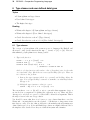
1.3.4 Practical examples
The following exercises will give you practice in creating and loading script files.
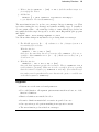
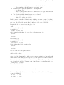
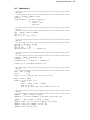
1. Create a file containing the following two lines. Each is a Haskell definition. Save
the file as Ex1.hs
add x y = x + y
square x = x * x
2. Until we load the new file, these definitions are not available for use. Try using
8
CSC3403 – Comparative Programming Languages
these functions; you should get an error as shown below.
Prelude> add 3 + 4
ERROR: Undefined variable "add"
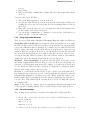
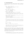
3. Now load the new definitions using the load (:l) command and then try using the
functions again.
Prelude> :l Ex1.hs
Reading file "Ex1.hs":
Hugs session for:
/home/rwatson/share/hugs/lib/Prelude.hs
Ex1.hs
Main> add 3 4
7
(14 reductions, 10 cells)
Hugs “remembers” which files are loaded. You only need to load a file once per session.
(A session begins when you start Hugs and ends when you exit Hugs.)
The message (14 reductions, 10 cells) tells how many computational steps (14
reductions) and how much space (10 cells) were required to calculate the result. This
message can be switched on with the :s +s Hugs command. The command :s -s
turns it off.
Hugs supports definitions spread over more than one file. In the following exercises we
will create a second file and include it in the Hugs session.
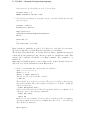
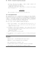
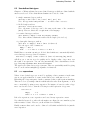
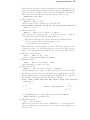
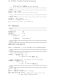
4. Create a new file Ex1a.hs containing the new definitions:
quad x = x * x * x * x
quad1 x = x ^ 4
quad2 x = square (square x)
and add it to the session with the command
:a Ex1a.hs
This will fail! Look at the error message. The reason for failure is that separate
files must be modules. The solution requires modifications to both files. To Ex1.hs
add the new first line
module Ex1(square) where
which creates and names the module and exports the definition for square. Now
add the two lines to the beginning of Ex1a.hs
module Ex1a where
import Ex1
Ex1a does not export anything, but it does import something (in this case square)
exported from Ex1. Now try again to add Ex1a.hs to the session — it should work!
Test out the new definitions:
Ex1a> quad 4
Laboratory Exercises
9
256
(12 reductions, 16 cells)
Ex1a> quad1 4
256
(47 reductions, 83 cells)
Ex1a> quad2 4
256
(13 reductions, 16 cells)
These alternative representations of quad illustrate a few points. First that there are
many ways to solve a problem and secondly that efficiency will vary with the method
selected.
The use of modules is a major departure from Gofer. Hence you will not see any
mention of modules in Wentworth. Haskell modules are quite flexible but we will not
explore all there features. For this course you should follow this basic scheme:
• Begin each file with module ModuleId exports where
where exports is optional and is a list of definition names inside parentheses:
(name1 , name2 , · · ·). If the exports list is not present, all definitions in the
module are exported.
• ModuleId must begin with an upper case letter.
• The name of the file should be ModuleId.hs, and the file name should begin with
an upper case letter.
• If module B uses a definition from module A, then module B must contain an
import directive: import A. A module can contain many import directives, and
each import directive can only refer to a single module.
For the simple problems encountered in the exercises, it is probably easiest to place all
your definitions in a single file without a module header. By default Hugs considers
this to be a module with name Main. You’ll see examples of the use of modules in the
SPL system.
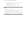
Hugs implements a concept called module chasing. The basic idea is that when you
load a module, any imported modules will automatically be loaded as well.
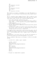
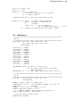
There are actually three different ways you could arrange to load the two modules Ex1
and Ex1a.
1. As described above, with two separate commands:
Prelude> :l Ex1.hs
Hugs session for:
/home/rwatson/share/hugs/lib/Prelude.hs
Ex1.hs
Ex1> :a Ex1a.hs
Hugs session for:
/home/rwatson/share/hugs/lib/Prelude.hs
Ex1.hs
Ex1a.hs
Ex1a> :q
2. Using the load command with two arguments
10
CSC3403 – Comparative Programming Languages
Prelude> :l Ex1.hs Ex1a.hs
Hugs session for:
/home/rwatson/share/hugs/lib/Prelude.hs
Ex1.hs
Ex1a.hs
Ex1a> :q
3. Using module chasing
Prelude> :l Ex1a.hs
Hugs session for:
/home/rwatson/share/hugs/lib/Prelude.hs
Ex1.hs
Ex1a.hs
Ex1a> :q
Which method you use is immaterial, as long as you understand what is happening.
A common strategy is to have a main module which imports many others. Then just
loading the main one will automatically load all the others.
Identifier visibility. You can refer to any identifier (a simple “variable” or a function
name) that is defined in the current module or is imported into the current module.
The current module is the one named in the Hugs prompt, which by default will be
Prelude>
but more likely
Main>
after you have loaded a module. If you have loaded a set of modules you can change the
current module with the Hugs :m command. This will enable you to refer to identifiers
in that module that perhaps had not been exported.
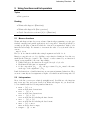
5. Try out some other features of the Hugs system:
1. Use the cursor keys to recall commands and to allow editing
2. (Only if you use :e to invoke the editor.)
Find definitions with :f. Note that this Hugs command requires that you
have configured or invoked Hugs to use an editor (the -E option to hugs). See
section 1.1. Furthermore, the editor must understand the +linenum option
so that it will start with the cursor on a specified line of the file.
• e.g. :f square
• try :f isUpper
can you see how it works?
• try out the supplied functions ord and chr
3. Find types with :t
• find the type of your definitions (e.g. :t square)
• find the type of system functions like isUpper
4. See how control-C works:
• type the expression [1..] (an infinite list)
• stop the display with control-C (or the stop button under Windows).
5. Finally, :? lists available commands and :q will end the Hugs session.
Laboratory Exercises
11
Key points
• Hugs is available under Linux and Microsoft Windows.
• There are two different ways to use the editor with Hugs.
• Scripts are added to Hugs sessions.
• Hugs remembers which scripts have been loaded during a current session.
• Explicit reloads are usually necessary after editing except if the edit session was
in response to a compile error.
• Multiple script files require use of explicit modules.
• Definitions must be exported from a module.
• All definitions in a module can be imported at once.
• control-C stops a runaway computation.
• :s can be used to control reporting.
12
CSC3403 – Comparative Programming Languages
2
Defining and Using Functions
Topics
• Writing simple Haskell definitions
• Local definitions and layout rules
• Tuples and simple patterns
Reading
• Wentworth section 2.4 (Layout)
• Gentle Introduction section 4.6 (Layout)
• Wentworth section 4.2 (Local Definitions)
• Gentle Introduction section 4.5 (Local Definitions)
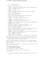
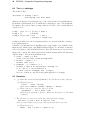
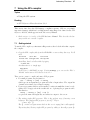
2.1
Introduction to function definitions
In Haskell, as in any functional programming language, the key programming element
is the function. Here is a simplified description of the format of functions. Local definitions (let expressions and where clauses) are used extensively in defining functions, so
appear in the description below. Later you will meet slightly more complex forms, but
the structure is identical. We use the extended BNF notation (see the text by Sebesta).
decl
f undecl
patdecl
rhs
where
expression
guardedRhs
→
|
→
→
→
|
→
→
|
|
|
|
→
f undecl
patdecl
varid pat∗ rhs [ where ]
pat rhs [ where ]
= expression
guardedRhs∗
where { decl [ ; decl ]∗ }
f unApplication
litteral
varid
if expression then expression else expression
let { decl [ ; decl ]∗ } in expression
| expression = expression
Notes
• A varid or variable identifier is a string of alphanumeric characters beginning
with a lower case alphabetic character. Unlike almost all other languages, the
case of the first character is important in Haskell: you have already seen that
module name must be begin with an upper case alphabetic.
• Examples of f unApplication are prefix expressions like square 4 and infix expressions like 1 + 2 and x > y. Note in all cases the lack of parentheses and
commas: in Haskell the space character separates a function and its arguments.
Thus the almost universal imperative language expression form of add(1,2) becomes add 1 2.) You’ll get used to it.
Laboratory Exercises
13
• The litteral above is any constant such as 42, 5.6, or "abc" (see Wentworth §2.2).
• Patterns will be covered later: for the moment we will consider only the simplest
pattern which consists of just a varid
• The declaration lists in let expressions and where clauses are shown separated
by semicolons and bracketed by braces. It is not usual to put them in your
programs. Instead, if you follow the layout convention (Wentworth §2.4), Hugs
will automatically insert them for you.
• When defining a set of functions, place the first character of the function name
in column 1. Otherwise the layout processor may not recognise all the functions
as “top level” (i.e. not local) definitions.
• Microsoft Windows users may encounter problems when creating script files that
depend upon the layout rules. Hugs always assumes an eight character indent
but some Windows editors do not. Actually the tab incompatibility is not just
a Windows problem, but is much less likely to occur in a Unix environment as
the eight character indent is a de facto standard. See section 1.3.3 for more
information.
2.2
Exercises
1. Start a new script file — you could call it Ex2.hs for instance. Add the following
lines to your script file.
mymin :: Int -> Int -> Int
mymin x y | x <= y
= x
| otherwise = y
This function returns the minimum of two integers. We had to call it mymin as min and
minimum are functions already defined in the standard prelude. Try it out.
Compare this definition with the grammar and identify the various components of the
definition. Note that otherwise is not a reserved word — it is merely a identifier
defined in the standard prelude as True.
2. Write a new version of the mymin function (mymin1) which uses an if expression
instead of the guarded expression form. Test it out.
The following function f takes two integers and returns a different answer depending
on the value of x. It includes a local definition.
3. Add this function to your script and try it out.
f :: Int -> Int -> Int
f x y = if x > 10 then x + a else x - a
where a = (y + 1) * (y + 1)
Note that the local variable a is used in two places in the if expression. Alternative
definitions of this simple function could use a let expression or guarded expressions.
Note also that we always add a type signature to each function definition. This is not
often necessary, but we do so as a useful discipline (you should always know in advance
the type of the function you are writing) and as a possible check on errors in coding
the function. If the signature and the function body conflict, Hugs will return an error.
14
CSC3403 – Comparative Programming Languages
4. Rewrite this function (call it f1) to use a let expression instead of a where clause.
5. Rewrite this function (call it f2) to use guarded expressions instead of an if expression. (You’ll still need the where clause).
There is often confusion over the use of let and where to introduce local definitions.
Usually they can be used interchangeably, as a matter of personal taste. For instance
the two following definitions are semantically equivalent:
x = let a = 5 in a + a
y = a + a where a = 5
However there are significant differences. The let reserved word introduces an expression. A let expression can appear anywhere that an expression is valid, such as an
argument to a function or as an expression being evaluated by the Hugs interpreter.
On the other hand, where introduces a clause which can only appear as a part of a
function definition or a case expression (Wentworth §2.6).
where clauses are particularly useful when used in conjunction with guarded function
definitions, because the definitions introduced by the where can apply to all the different guarded expressions. Otherwise, let expressions are generally more often used for
local definitions.
Note that the scope of variables defined by let or where constructs includes the right
hand sides of all the definitions. That is, any local variable defined by a let of where
can appear in the definition of another variable within the same set of local definitions.
Here are some more exercises to attempt.
6. Write the two companion functions
hextonum :: Char -> Int
numtohex :: Int -> Char
Which convert between a hexadecimal character and a decimal number (an integer). The hexadecimal char is one of 0123456789abcdefABCDEF, and the integral
value will in the range 0–15. You can use the prelude functions ord::Char->Int
and chr::Int->Char; these convert between a character and its equivalent ASCII
code.
Test your functions. See if they work for all numbers by evaluating the expression
map (hextonum . numtohex) [0..15]
Note: don’t create a simple (but also correct) solution where you just enumerate
all possibilities. Such a solution would look in part like:
hextonum ’8’ = 8
hextonum ’9’ = 9
hextonum ’A’ = 10
hextonum ’B’ = 11
The following two exercises use tuples. A tuple is like a record or structure whose fields
have no names. A tuple value is constructed simply with parentheses and commas, and
can be any length and contain any mixture of types:
Laboratory Exercises
15
x = (101,"Frank")
y = (True, 1, 2, ’c’)
z = ((1,2), (’a’,5.3,42))
To access these values we use pattern matching. For instance to access the elements of
a pair we could define (as is done in the prelude)
fst (a,b) = a
snd (a,b) = b
The (a,b) part is the pattern: a matches the first item in the tuple and b matches the
second item in the tuple.
7. Write the function
later :: (Int,Int,Int) -> (Int,Int,Int) -> Bool
which returns True if the first date is later than the second. The (Int,Int,Int)
arguments are interpreted as (day, month, year). Test it.
8. Write a function to calculate a person’s age in whole number of years given a
birth date and the current date
age :: (Int,Int,Int) -> (Int,Int,Int) -> Int
This is interpreted as: (d, m, y) → (d, m, y) → years
2.3
More on let expressions
When should we use let expressions (or where clauses)? Here are three situations:
• to implement a sequence of operations,
• to simplify a complex expression, and
• to provide pattern matching.
Here is an example that uses a let expression to simplify and sequence the evaluation
of an expression. We could write
f a = (((a + 5) * 3) / 7) + 1
or we could write the equivalent:
f a
= let b
c
d
in d
=
=
=
+
a + 5
b * 3
c / 7
1
The first definition forces sequencing of sub-expression evaluation using parentheses,
while the second uses data dependencies to produce the same sequence of evaluation. Note that the second evaluation c = b * 3 cannot be performed until the first
(b = a + 5) is evaluated, thus yielding a value for b. The variables c and d play a
similar role in sequencing the final two expression evaluations.
The second definition is somewhat clearer, as one does not need to study the nesting
of parentheses to determine evaluation order, but many programmers would argue that
it is an inferior definition in that it is not as concise as the original definition. Often
16
CSC3403 – Comparative Programming Languages
it is easier to develop a let-based definition at first, then possibly rewrite it in a more
compact form (possible using the functional composition operator — see section 5.1).
Pattern matching is an essential part of functional programming — it enables us to
extract and inspect the component parts of structured data such as tuples and lists.
Imagine that you are writing a function to calculate the vector describing the relative
positions of two objects on a plane. You could write
vec x y = let (a,b) = get_coordinates x
(c,d) = get_coordinates y
in (c-a, d-b)
The let expression here allows is the split up and sequence the two lookup operations,
then extract the x and y coordinates that they return. As a final note, be aware that
pattern matching can occur equivalently when an argument is defined or within a let
expression. So the definition of fst above, which was written as
fst (a,b) = a
could also be written as
fst x = let (a,b) = x
in a
Sometimes this approach is used when an argument has a complex structure.
Key points
• There are two forms of function definition.
• where clauses and let expressions are similar.
• where clauses and let expressions are different.
• Guarded functions can be written using (possibly nested) if expressions.
• A function written a where clause can usually (but not always) be written using
a let expression.
• Tuples can be of any length and contain any types.
• Tuple argument values are accessed via patterns.
• The layout rule is a syntactic convenience allowing cleaner function definitions.
Laboratory Exercises
3
17
Pattern matching and recursion
Topics
• Defining patterns
• Recursion with integers and lists
• Case expressions
Reading
• Wentworth section 2.3 (Lists and strings)
• Wentworth section 2.5 (Patterns)
• Wentworth section 2.6 (case expressions)
• Gentle Introduction sections 4[.0] – 4.4 (case expressions and patterns)
• Gentle Introduction section 3.5 (Error function)
Be sure to read the sections from Wentworth before proceeding with this laboratory.
3.1
Patterns
The use of patterns is a key departure from most imperative languages. The pattern
plays a similar rôle to that of the imperative language’s formal parameter but with
some significant differences.
1. A formal parameter is a single identifier, while a pattern can be a complex expression involving many identifiers.
2. An imperative argument (actual parameter) is always bound to its formal parameter at call time — in Haskell, the binding of argument to pattern only occurs
if the pattern matches the structure of the argument. Thus a set of function
definitions is commonly written to handle various possible argument structures.
The definitions are tried in strict top to bottom order until a match is found,
otherwise a fatal program error occurs.
3.2
Recursion
Writing recursive functions can be challenging at first. The best way to proceed is to
first look at some recursive definitions. See Wentworth §2.5 for some initial samples.
The Hugs standard prelude abounds with more examples.
All recursive definitions have some common features which you should recognise and
emulate when you begin writing your own.
1. There is always at least one (but often just one) base case. The base case is
the expression within the function body (right hand side) which is not recursive.
That is, the base case does not call itself. Usually the base case is represented by
a complete function definition, but it may be part of an if or case expression.
18
CSC3403 – Comparative Programming Languages
2. There is always at least one function definition which includes a recursive call.
This recursive call must result in a smaller amount of calculation occurring, or else
the function will never complete (the functional equivalent of an infinite loop).
“Smaller” can mean a smaller number (as in the standard factorial example) or
a smaller structure (as used in list processing functions).
Writing a recursive function involves identifying the base case, and the recursive case(s).
The recursive case is usually the most difficult to write. It is often an expression
involving two subexpressions: one subexpression is the recursive call while the other is
some expression related to that “part” of the argument which is not being passed on
to the recursive call. This last statement is necessarily somewhat vague, so let’s look a
a couple of examples. For instance in the following factorial example
fact n = n * fact (n-1)
and also one which calculates the length of a list
length (x:xs) = 1 * length xs
the two subexpressions are identified. Note that in the second example the expression
1 is “related to” the argument pattern x — the length of x is 1.
3.3
Case expressions
case expressions provide absolutely equivalent pattern matching features to those available via function definitions. They are very handy alternative to constructing “throw
away” functions (used once only). They are particularly useful also in dealing with user
defined data types (see Laboratory 6).
The two expressions below are equivalent, though the case expression is tidier:
let
f pat1 = expr1
....
f patn = exprn
case arg of
pat1 -> expr1
....
patn -> exprn
in
f arg
3.4
Exercises
Open a new script file and add definitions for the functions specified below. You may
also wish to type in the definitions from the examples in Wentworth §2.5 and test them.
1. Write the recursive function multiply :: Int -> Int -> Int which multiplies
two positive numbers together by successive addition. That is, use the + (and -)
operators but not the * operator. Test it. Be sure it handles multiplication by
zero.
2. Your solution probably works more slowly in one of these cases:
multiply 1 10000
multiply 10000 1
(Use the Hugs command :s +s to turn on reduction counting.) How would you
modify the the function so that both expressions evaluated in approximately the
same number of reductions?
Laboratory Exercises
19
3. Write a function smallest :: [Int] -> Int to find the smallest integer in a
(non empty) list. Test it.
4. Add the line
smallest [] = error "smallest: list must be non-empty"
to you definition. Test it with smallest [].
The error function is used to produce error messages. Its type is String -> a. That
is, it takes a string (the error message) and returns something of type a. Actually it
does not return a value — the return type is there to ensure that the type checker can
successfully check the script. In response to a call to error, Hugs will stop the program
and display
Program error: error message argument to error
You can use this technique in any function for producing fatal error messages.
5. The Haskell expression [m ..
incrementing by 1 each time.
n] evaluates to a list of integers from m to n
Write the function
enumList :: Int -> Int -> [Int]
which does the same thing but uses a recursive call to enumList. (It is not acceptable to define enumList m n = [m .. n].) Make sure it works for m ≥ n
as well as m < n.
6. Write the function
enumList1 :: Int -> Int -> Int -> [Int]
where the third argument specifies the increment. That is, enumList1 2 12 4
would evaluate to [2,6,10]. Make sure it works correctly in all cases, especially
when the interval is negative (e.g. enumList1 2 12 (-4)). (Note that the negative number must be parenthesised because otherwise the operator - would be seen
as the third argument to enumList1).
Key points
• Patterns are not the same as formal parameters.
• For a valid function: all argument patterns must match in at least one of the
function’s definitions.
• Function definitions are matched in order.
• Recursive definitions must include a recursive step and a base case.
• Case expressions provide pattern matching in an expression context.
• The error function produces fatal error messages.
20
CSC3403 – Comparative Programming Languages
4
Debugging, Recursion, List comprehensions
Topics
• Debugging
• Recursive list processing functions
• Styles of recursion
• List comprehensions
Reading
• Wentworth section 3.1 (Polymorphism)
• Wentworth chapter 4 (Recursive programming)
• Wentworth chapter 7 (List comprehensions)
• Gentle Introduction section 2.4.1 (List comprehensions)
4.1
Debugging
Debugging functional programs can be challenging as, compared with imperative languages, there are no symbolic debuggers available and the C-style printf debugging
message technique is not applicable.
There are a couple of very rudimentary debugging techniques using the standard prelude functions error and trace, but these are not very useful as they either halt the
program or force unwanted evaluation of expressions. Fortunately the recently introduced observe function can be a very useful debugging tool.
Hugs has been modified to support a special primitive or built-in function called
observe. Its type signature is
observe ::
String -> a -> a
The partial application
observe tag
behaves exactly like the “do nothing” identity function 1 , but also records the value of
expressions to which it is applied. Any observations made are reported at the end of
the computation. The tag argument is a string that is used to label the observed value
when it is reported.
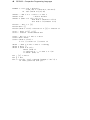
Let’s look at a simple example, a solution to the first exercise of the previous module:
multiply
multiply
multiply
multiply
1
:: Int -> Int -> Int
0 b = 0
1 b = b
a b = b + multiply (a - 1) b
id x = x
Laboratory Exercises
21
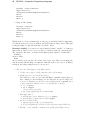
Imagine we wanted to look at the value of the first argument to multiply. We could
change the definition to read
multiply a b = b + multiply (observe "a" a - 1) b
You must also add the directive
IMPORTANT:
import Observe
into the script (typically on the first line following the module
header) in order to use the observe function.
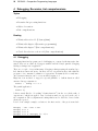
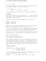
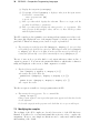
Running a test will now give the result:
Main> multiply 5 2
10
>>>>>>> Observations <<<<<<
a
5
4
3
2
which shows the result of the computation (10) as well as all the argument values
(except 1, which is handled by a separate definition).
More usefully, we can actually observe the arguments and result of a function. If we
use this definition:
multiply a b = b + observe "mult" multiply (a - 1) b
then we can “see” the behaviour of multiply. For instance:
Main> multiply 5 2
10
>>>>>>> Observations <<<<<<
mult
{ \
, \
, \
, \
}
4
3
2
1
2
2
2
2
->
->
->
->
8
6
4
2
Note that it is quite acceptable to have multiple observations in a script. For instance
the two examples above could be combined:
multiply a b = b + observe "mult" multiply (observe "a" a - 1) b
22
CSC3403 – Comparative Programming Languages
The observe system also respects lazy evaluation. For instance we can observe an
infinite list without evaluating it. If the definition
inf = observe "infinite list" [1..]
is in scope then we would see the following result:
Main> take 5 inf
[1,2,3,4,5]
>>>>>>> Observations <<<<<<
infinite list
(1 : 2 : 3 : 4 : 5 : _)
The _ symbol indicates an unevaluated list tail.
1. Try using observe within a script that you have written. Make sure you use
observe to observe both values of expressions and the behaviour of functions.
4.2
Recursion styles and efficiency
Read carefully Wentworth chapter 4 as it covers some key issues. Take time to read and
understand the examples, each of which contains a base case and recursive step. Note
that Wentworth uses the equivalent term “inductive case” to describe the recursive
step.
The difference between backward and forward recursion can be difficult to see but are
very important from an efficiency point of view, especially when dealing with lists. The
primary efficiency problem concerning lists is that adding a item to the front of a list
is much cheaper than adding an item to the end of a list. Prepending with the colon
or “cons” operator (e.g. x:xs) is very cheap and its cost is the same irrespective of the
length of the list. However adding to the end with the append operator (e.g. xs ++
[x]) requires that n cons operations be carried out, where n is the length of xs. So
repeated appending to a list is very expensive.
When testing different solutions (especially comparing different recursion styles) turn
on reduction count reporting with the Hugs command :s +s and note the reduction
counts.
The following exercise illustrates the different cost of cons and append.
2. Create a new script file containing just the definition
xs=[1..100]
and load it into your Hugs session. Turn on reduction counting. Type length xs.
Do it again. You should note a smaller reduction count the second time because
Hugs has remembered that the expression [1..100] reduces to a 100-item list.
Now check the reduction counts for the expressions
length (1:xs)
and
length(xs++[1]).
What is the difference in the reduction counts? Can you explain why the “cost”
of adding an item to the beginning of a list differs from that of adding to end?
Laboratory Exercises
4.3
23
List processing exercises
Try the following exercises. List processing is at the heart of almost every functional
programming application. You must develop the ability to easily program such applications.
3. count :: String -> Char -> Int
Count occurrences of a character in a string. For example
count "abc-xyz-55-$-X" ’-’ ⇒ 4
count "Alphabet" ’a’ ⇒ 1
4. cpy :: Char -> Int -> String
Make a string of n characters. For example
cpy ’Z’ 10 ⇒ "ZZZZZZZZZZ"
5. spaceIt :: String -> String
Place space characters between characters in a string. For example
spaceIt "Hello, world" ⇒ "H e l l o ,
w o r l d"
Be careful not to include a leading or trailing space character. (This is hard to
see — for testing purposes, insert a visible character like ’_’ instead of a space.)
6. countS :: [Char] -> String -> Int
countS chars string counts the total number of all characters in char which
appear in string. For example:
countS "ab" "xaxbxccxaab" ⇒ 5
That is, the sum of the number of ‘a’ characters and the number of ‘b’ characters
is 5.
7. Look at Wentworth program fragment 4.9 which converts a decimal number into
a string of binary digits using backward recursion. This will not work in Haskell
because the / operator cannot be used for integer division. Using div instead we
have
bin :: Int -> [Int]
bin 0
= []
bin n | n > 0 = bin (n ‘div‘ 2) ++ [n ‘mod‘ 2]
Add this definition and test it. Then rewrite it using forward recursion. Use
fragment 4.4, the forward recursive version of reverse as a model for this. You
will need to add an extra “accumulating” argument.
The notation ‘div‘ in the last example deserves some comment. A function is usually
employed as a prefix operator. So div n 2 is the result of dividing n by 2. Sometimes
we might prefer, for the sake of readability perhaps, to use the function name in an infix
context, just like a binary operator. In this case the function name must be quoted
with back quotes. The converse is also possible: parenthesised operator symbols may
be used in an infix expression as in (+) n 2.
8. Challenge question Normal computer integer arithmetic is limited by the word
size of the machine. By representing numbers as lists of integers we can ignore
24
CSC3403 – Comparative Programming Languages
these limits. Write the function addStr :: [Int] -> [Int] -> [Int] to add
two such list representations. For instance
addStr [6,5,7,6] [1,4,7]⇒ [6,7,2,3]
You will need to use the rules for adding numbers one column at a time, keeping
track of carry digits, e.g.
6 5 7 6
11 41 7
6 7 2 3
Hint: use reverse so that strings can be processed right to left.
4.4
List comprehensions
List comprehensions are a very convenient form of specifying some forms of list functions. For these cases they are much shorter, clearer, and simpler because the list does
not have to be laboriously deconstructed and reconstructed. Chapter 7 of Wentworth
contains a good description with numerous examples. Make sure you understand the
rôle of the generator and filter expressions in constructing a list.
Here are a couple of exercise originally from Wentworth chapter 4.
9. Write a function proper :: Int -> [Int] which lists the proper factors of a
number. The proper factors of n are all its factors except 1 and n. For instance
proper 12 ⇒ [2, 3, 4, 6]
10. Use proper to write the function isPerfect :: Int -> Bool, which checks if
its argument is a perfect number. A positive number is perfect if its proper factors
sum to one less than itself. For example:
isPerfect 6 ⇒ True
Hint: use the sum function from the prelude.
11. Use isPerfect in a list comprehension expression to list the first three perfect
numbers.
Key points
• Functions can be coded with backward and forward recursion.
• Efficiency of cons (:) and append (++) are very different.
• List comprehensions are powerful and concise.
• A function which is defined for an argument of any type is polymorphic.
• Type signatures for polymorphic functions contain type variables.
Laboratory Exercises
5
25
Using functions and list operators
Topics
• List operators
Reading
• Wentworth chapter 8 (Functions)
• Wentworth chapter 10 (List operators)
• Gentle Introduction sections 3[.0]–3.3 (Functions)
5.1
More on functions
Wentworth chapter 8 introduces some advanced functional programming concepts, particularly currying (and partial application) and composition. Currying is handy for
creating special purpose functions, which are often used as arguments to higher order
functions such as map. For instance to increment the value of every item in a list we
can use
map (+ 1) xs
Here (+ 1) is a function which takes a single argument and adds 1 to it.
Function composition is a tool for building concise function definitions. It works very
much like the Unix pipe | symbol. The “output” or value returned by one function is
“input” as an argument to the next. Importantly:
• Unlike Unix pipes, the functions are applied in right to left order
• Each function takes just one argument
• for the composition f un2 . f un1 , the type returned by f un1 must be the same
as the type of the argument to f un2 .
Lambda abstractions, or lambda functions, are anonymous (unnamed) functions. They
are most commonly used as arguments to higher order functions such as map and fold.
5.2
List operators
Most of the list operators are relatively straightforward. In addition to the functions
map, fold, any, all, and elem described in Wentworth chapter 10, you should also
become familiar with the following standard functions.
• head :: [a] -> a
head xs is the first element in xs
• last :: [a] -> a
last xs is the last element in xs
• tail :: [a] -> [a]
tail xs is the list xs excluding the first element
• init :: [a] -> [a]
init xs is the list xs excluding the last element
• null :: [a] -> Bool
null xs is true if xs is empty
• length :: [a] -> Int
26
CSC3403 – Comparative Programming Languages
• (!!) :: [b] -> Int -> b
xs !! n is the nth item in xs
• iterate :: (a -> a) -> a -> [a]
iterate f x is the list whose first item is x and each item is calculated from the
previous by applying the function f to it.
• repeat :: a -> [a]
replicate :: Int -> a -> [a]
repeat a is an infinite list of a; replicate n a is a finite list of length n
• take :: Int -> [a] -> [a]
take n xs is the first n items in xs
• drop :: Int -> [a] -> [a]
drop n xs is the last items in xs after removing the first n items
• splitAt :: Int -> [a] -> ([a], [a])
splitAt n xs is equivalent to (take n xs, drop n xs)
• takeWhile :: (a -> Bool) -> [a] -> [a]
takeWhile p xs is those initial elements of xs satisfying p
• dropWhile :: (a -> Bool) -> [a] -> [a]
dropWhile p xs is the final elements of xs remaining after all initial elements
satisfying p have been removed
• span, break :: (a -> Bool) -> [a] -> ([a],[a])
span p xs is equivalent to (takeWhile p xs, dropWhile p xs)
break p xs is equivalent to span (not . p) xs
• zip :: [a] -> [b] -> [(a,b)]
zip xs ys is a list of pairs formed by taking corresponding items from xs and
ys. If one list is longer than the other, the extra items are ignored.
• zipWith :: (a->b->c) -> [a]->[b]->[c]
zipWith f xs ys is a list formed using f create item from the members if xs
and ys. For instance zip is usually defined as
zip = zipWith (\a b -> (a,b))
• unzip :: [(a,b)] -> ([a],[b])
unzip is the inverse of zip (as long as the original lists were of equal length).
These functions are a vital part of the functional programmers “tool kit”. You can
write programs without using them, but you will often end up “reinventing the wheel”
— effectively writing your own versions of these functions.
If in doubt about the meaning or these functions, look in the standard prelude to
find their definitions. These definitions are quite short and are valuable examples of
functional programs.
You’ll also find other definitions there: you should also look at these as we’ve only
listed the most common one here.
5.3
The fold family of operators
The fold functions can be hard to understand
I like to think that fold works as follows. Consider the expression
fold f a xs
• here fold takes as argument a list (xs) but returns a value which is not necessarily
a list.
Laboratory Exercises
27
• the argument a is an initial approximation to the final value of fold f a xs
– this means that a has the same type as fold f a xs
• fold arranges to apply its argument f to two arguments
– an element of xs
– either a or an updated version of a, which is a better approximation of the
final result of fold f a xs
• The order in which the items of xs are processed can be
– left-to-right: in the case of foldl
– right-to-left: in the case of foldr
I find it easiest to visualise fold functions by thinking of f as an operator. Note that f
must take two arguments, one has the type of the list elements and the other has the
type of a. The order of the two is different in the two fold cases (foldl/foldr).
Imagine that the + operator is used in place of f
Then
foldl (+) 0 [1,2,3]
is equivalent to
(((0 + 1) + 2) + 3)
notice that each application of + gets closer to the final result of 6:
0+1 ⇒ 1
1+2 ⇒ 3
3+3 ⇒ 6
foldr is analogous:
foldr (+) 0 [1,2,3]
is equivalent to
(1 + (2 + (3 + 0)))
but it evaluates the list in opposite order
3+0 ⇒ 3
2+3 ⇒ 5
5+1 ⇒ 6
Note also that the foldl applications are
a’ + x
while for foldr we have
x + a’
where x is a list element and a’ is the most recent approximation of our final result,
which started as the value (a) and is updated by each application of the fold function.
The + function takes two arguments of the same type. This will not generally be the
case. Consider the problem of turning a list of integers into an equivalent string. e.g.
conv [1,2,3] ⇒ "123"
We can do this with foldr
conv s = foldr f "" s
where f i s = chr (i + ord ’0’) :
s
Then conv [1,2,3] evaluates foldr f "" [1,2,3] which results in the following sequence of applications
f 3 ""
⇒ "3"
f 2 "3"
⇒ "23"
28
CSC3403 – Comparative Programming Languages
f 1 "23"
⇒ "123"
You cannot use the same f for both foldr and foldl when the function is not symmetric
(+ is symmetric) Rewriting conv to use foldl would require
conv s = foldl f "" s
where f s i = s ++ [chr (i + ord ’0’)]
Note that the arguments to f are in a different order, and the body is different also.
5.4
State
In an imperative language you can update data “in situ” — a data item is simply
replaced by the new value. Thus a hypothetical C program to maintain a database of
phone numbers could include the lines
void add(char *name, char *phone, phoneDB *db);
...
add("me", "1234", db);
add("her", "2345", db);
add("him", "3456", db);
/* prototype */
which successively adds (name, phone number) pairs to a database of phone numbers.
After each statement the database identified by db will have a new value.
We can’t do this in a functional program — all functions must return values, and
besides an identifier, which is called a variable in the mathematical sense rather than
the traditional programming sense, can only be assigned a single unique value.
Instead we write a state transformer which takes an initial state (the phone database)
and returns a new state, or new version of the old one. For instance we could define:
type DB = [(String,String)]
add :: String -> String -> DB -> DB
add name phone db = (name,phone) : db
(The type declaration just introduces a new type name DB which is a synonym for the
type which appears following the equals symbol — see Wentworth chapter 6.) Note
that the function takes as argument a state (DB) and returns the updated state. It is
a state transformer because the state is changed by the application of the function.
We can rewrite our C example, which performs a sequence of updates, in a number or
ways.
Using let expressions.
addmany db = let db’ = add "me" "1234" db
db’’ = add "her" "2345" db’
in
add "him" "3456" db’’
We have to keep track of each new (intermediate) state. The function addmany :: DB -> DB
is itself a state transformer. It would be used like this:
addmany []
⇒
[("him","3456"), ("her","2345"), ("me","1234")]
Laboratory Exercises
29
Using composition. In the following definition note that expressions of the form
add "him" "3456" have type DB -> DB and so we can string as many as we like together with the composition operator.
addmany’ db = add "him" "3456" . add "her" "2345" . add "me" "1234" $ db
The $ operator is an application operator. It says “apply the function on the left to
the argument on the right”. In this case the function on the left is
add "him" "3456" . add "her" "2345" . add "me" "1234"
and the argument is db. We could also have written the (slightly less readable perhaps):
addmany’ db = (add "him" "3456" . add "her" "2345" . add "me" "1234") db
Using fold. Finally we could use foldl to add items from a list of (name,number)
pairs to the database. Note that we need to introduce a new local function f which
simply marshals the arguments to add in the order expected by foldl before calling
add.
addmany’’ db = foldl f db [("me","1234"),("her","2345"),("him","3456")]
where f db (name,phone) = add name phone db
The fold version has the advantage that it (addmany’’) can be abstracted to create
addlist, which will handle any length of list.
addlist ps db = foldl f db ps where f db (name,phone) = add name phone db
addmany’’’ db = addlist [("me","1234"),("her","2345"),("him","3456")] db
This form of abstraction is common in writing Haskell programs.
Which form of state update you use is not that important — mostly it will depend
upon context. What is more important is that you recognise when you are dealing
with state and state transformers so that you can program appropriately. In particular
note that the compositional approach will only work with functions which have type
State → State. The order of the parameters in the add function is important; the
State parameter must be the final one in the list of parameters.
5.5
Exercises
1. Define a
lexord
lexord
lexord
function lexord :: String -> String -> Int
s1 s2 ⇒ -1 if s1 < s2
s1 s2 ⇒ 0 if s1 = s2
s1 s2 ⇒ 1 if s1 > s2
lexord is a “dictionary” ordering function. That is:
lexord "abc" "def" ⇒ -1
lexord "abc" "abd" ⇒ -1
lexord "abc" "ab" ⇒ 1
lexord "abc" "abcd" ⇒ -1
lexord "abc" "abc" ⇒ 0
2. Using foldl together with the system function max write the function
maxS :: [Int] -> Int
to find the maximum value in a non-empty list.
30
CSC3403 – Comparative Programming Languages
3. Using foldr together with the system function min write the function
minS :: [Int] -> Int
to find the minimum value in a non-empty list. Look up the foldr1 function in
the standard prelude and recode minS as minS’ using this version of fold.
4. Use foldr to define the function
remdups :: [Int] -> [Int]
which removes duplicate entries from a list.
Hints
• The function will take the form
remdups s = foldr f [] s
where f ? ? = ....
....
That is, your task is to write the local definition for function f ( the ? shows
where an argument pattern will appear).
• Here is a simple recursive version you may wish to use for inspiration.
remdups [] = []
remdups [x] = [x]
remdups (x:y:ys) = if x==y then remdups (y:ys)
else x : remdups (y:ys)
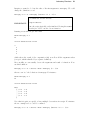
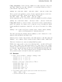
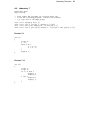
5. Define functions to calculate and display Pascal’s triangle
1
1 1
1 2 1
1 3 3 1
1 4 6 4 1
1 5 10 10 5 1
1 6 15 20 15 6 1
1 7 21 35 35 21 7 1
You will need (at least) two functions
(a) pasc :: Int -> [[Int]]
pasc n will produce the numbers in the first n rows of the triangle. For
example:
pasc 3 ⇒ [[1],[1,1],[1,2,1]]
Hint
There is a simple computational method for generating any line from its
successor. Consider generation of the fourth line from the third
1 2 1 0
+ 0 1 2 1
1 3 3 1
Try using zipWith to describe this algorithm. E.g.
nextrow :: [Int] -> [Int]
nextrow xs = zipWith ...
Note that the zeros are added to the beginning and ending of the same string
of numbers.
Laboratory Exercises
31
(b) This is a difficult problem.
prpasc :: [[Int]] -> [String] takes the list of numbers generated by
pasc and prints them as shown above.
• the problem involves (at least)
– formatting each line (format :: [Int] -> String)
– determining the longest (formatted) line
– centering all but the longest line by padding the beginning of the line
with spaces
• you may wish to define and use the function
catWith sep (xs:xss) = foldl (\a b->a++sep++b) xs xss
e.g. catWith " " (map show [1,2,3]) ⇒ "1 2 3"
• use the I/O function putStr to display your output, e.g.:
(putStr . prpasc . pasc) 5
Key points
• Partial applications (via currying) and lambda abstractions are a useful way of
generating “anonymous” functions.
• Function composition can “glue” a sequence of functions together.
• There are many standard functions in the functional programmers tool kit.
• Using a fold function can greatly simplify some kinds of list processing functions
— but you must be able to recognise when it can be employed.
• Updating state by state transforming functions is fundamental to functional programming.
32
CSC3403 – Comparative Programming Languages
6
Type classes and user defined data types
Topics
• Polymorphism and type classes
• User defined data types
• The Maybe data type
Reading
• Wentworth chapter 3 (Polymorphism and type classes)
• Wentworth chapter 6 (User defined data types)
• Gentle Introduction section 5 (Type classes)
• Gentle Introduction section 2.2–2.4 (User defined data types)
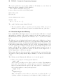
6.1
Type classes
The concept of polymorphism adds enormous power to languages like Haskell, and
allows us to write generic functions like map :: (a->b) -> [a] -> [b]. However,
this unlimited polymorphism is not always possible.
1. Type in the function
search :: a -> b -> [(a,b)] -> b
search k fail []
= fail
search k fail ((a,b):xs) | k == a
= b
| otherwise = search k fail xs
which is a lookup function with searches a list of (key,value) pairs for the value
associated with a key. Check the error message that Hugs gives you. There are
two solutions to the problem:
1. Remove the type signature (which is too general) and let Hugs deduce the
type. You can type the Hugs command :t search to see what Hugs believes
the type to be.
(a) Modify the type signature so that it is correct:
search :: Eq a => a -> b -> [(a,b)] -> b
The reason that a -> b -> [(a,b)] -> b is too general is that arguments of type a
are involved in a comparison for equality (the expression k == a). Thus only those
data types for which the == operator is defined will be allowable as arguments. This is
the major reason for the use of type classes.
You should be aware that there is a lot more to type classes than that covered in
Wentworth — in particular how are they defined — but this is not of importance in an
introductory course. Note also that we will refer to them further when discussing user
defined data types below. Gofer and Haskell type classes are slightly different, but for
the simplest cases described here they are identical in syntax and semantics.
Laboratory Exercises
6.2
33
User defined data types
Chapter 6 of Wentworth introduces user defined data types, which are defined with the
data reserved word. Notice that this mechanism can be used to define
1. simple enumerated types, such as
data Day = Sun | Mon | Tue | Wed | Thu | Fri | Sat
Note: the type name is Day and Sun ... as called a data constructor
2. labelled tuples, such as
data Rect = Rect Float Float
Note: the name of the type can be the same as the name of the constructor
(Rect). However, this is not a requirement of the language.
3. recursive data types, such as
data IntTree = Empty | Node Int IntTree IntTree
Note: this combines enumeration with a labelled tuple (1 & 2 above)
4. polymorphic data types, such as
data Tree a = Empty | Node a (Tree a) (Tree a)
Note the types of the constructors:
Empty :: Tree a
Node :: a -> Tree a -> Tree a -> Tree a
Haskell has a convenient extension to Gofer’s data definitions to automatically include
a new data type in a type class. For instance
data Tree a = Empty | Node a (Tree a) (Tree a) deriving (Eq, Show)
will allow you to test two trees for equality and to display a value of type Tree a as
the result of an expression. You can only automatically derive class instances for the
type classes Eq, Ord, Enum, Show, Read, and Bounded.
The type keyword introduces a type synonym. These are particularly useful for giving
a more concise and meaningful type signature for functions.
6.3
case expressions
Values of user defined types are created by applying a data constructor in the same
way as you apply a function. So Node 4 Nil Nil is a tree with just one node.
Extracting the component parts of such a constructed value requires pattern matching.
This can be done by writing a function which takes the value as an argument, or often
more conveniently by using a case expression. For instance, if tree is a value of type
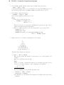
Tree a as described above, then the following is a valid expression of type Int:
case tree of
Empty
-> 0
Node v l r -> 1 + tSize l + tSize r
Like a let expression, a case expression can be used in any expression context.
Note that the layout above where the alternatives are aligned is a not mandatory, but
rather a matter of taste. However you should aim for readability.
Finally, a where clause can be used to define a local definition which holds for just the
case expression.
34
CSC3403 – Comparative Programming Languages
6.4
The Maybe data type
The prelude defines
data Maybe a = Nothing | Just a
deriving (Eq, Ord, Read, Show)
which is very handy for describing the type of the value returned by a partial function.
Recall that a partial function is one which has no mapping fro some of its arguments.
For instance the prelude defines lookup, which is a version of the search function
described above.
lookup :: Eq a => a ->
lookup k []
=
lookup k ((x,y):xys) |
|
[(a,b)] -> Maybe b
Nothing
k==x
= Just y
otherwise = lookup k xys
lookup is undefined for some key arguments (those not present in the list of pairs) so
it is a partial function.
A number of useful functions for handling values of type Maybe a are available in the
Maybe module, which is part of the Haskell Standard Library. See the Hugs documentation for description of the Standard Library modules. The functions are exported from
Maybe, and so any module which employs such a function must include the statement
“import Maybe”. The most useful functions are
• isJust :: Maybe a -> Bool
isJust (Just x) is True, isJust Nothing is False
• fromJust :: Maybe a -> a
fromJust (Just x) is x
• fromMaybe :: a -> Maybe a -> a
fromJust a (Just x) is x and fromJust a Nothing is a
So, we could recode our search function as
search’ k fail = fromMaybe fail . lookup k
(note use of function composition and partial application of lookup).
6.5
Exercises
2. (a) Define the enumerated datatype Month to describe the 12 months of the year.
(b) Write the function
season :: Month -> String
which returns "Summer", "Autumn", "Spring", or "Winter".
(c) Write a function to return the days in a month
daysInMonth :: Int -> Month -> Int
where the first argument is the year. Make sure the function is Year 2000
compliant!
3. The following set of exercises involve the polymorphic Tree datatype
data Tree a = Node a (Tree a) (Tree a) | Nil
which you must define in your script. Add any derived classes you need.
(a) Write the function
minMax :: Ord a => Tree a -> Maybe (a,a)
Laboratory Exercises
35
which traverses the tree to find the minimum and maximum values it contains. Note that testing the empty tree with the expression minMax Nil will
produce an error — the type checker can’t work out what kind of tree Nil is.
The solution is to provide some extra information, in the case say:
minMax (Nil::Tree Int)
(b) Write the function
flatten :: Tree a -> [a]
which performs a left to right traverse of the tree. E.g.
flatten (Node 1 (Node 10 Nil (Node 2 Nil Nil)) (Node 4 Nil Nil))
⇒[10, 2, 1, 4]
(c) Write the function
sInsert :: Ord a => a -> Tree a -> Tree a
which performs an ordered insertion of an item into the tree, so that the
node values in the tree meet the following condition:
If maxV al t and minV al t are the maximum and minimum values
of nodes in tree t, then for the node Node v t 1 t2
v ≥ maxV al t1 ∧ v < minV al t2
Hint: The heart of the algorithm is as follows. To insert a value at a node:
compare the value to be inserted against the current node value; if insert
value ≤ node value then insert in left sub-tree, else insert in right sub-tree.
(d) Write the sorting function
tsort :: Ord a => [a] -> [a]
in terms of only flatten, foldr, and sInsert.
(e) Write the function
telem :: Eq a => a -> Tree a -> Bool
which determines if a value is in a tree.
(f) Write the function
showT’ :: Show a => Int -> Tree a -> String
which prettyprints a tree. One node value is printed per line, with each value
preceded by a number of spaced determined by its depth in the tree. The
integer argument is the “current indent level”, initially set to 0. Increase
the indent by 4 characters per level. For instance the tree
Node 3 (Node 2 (Node 1 Nil Nil) Nil) (Node 5 (Node 4 Nil Nil) Nil)
would appear as
3
2
5
1
(which is equivalent to)
4
3
/ \
2
5
/
/
1
4
Use the putStr function to display the string generated by showT’:
putStr (showT’ 0 tree-expression)
(g) Write the function
bal :: [a] -> Tree a
which takes a sorted list and creates a balanced tree. A balanced tree has
the property that the size of both subtrees of a node are equal or differ in size
by at most one.
36
CSC3403 – Comparative Programming Languages
Hint: Recursively split the input list in half, using bal to build the subtrees
before creating the node.
Compare the result of balanced and unbalanced insertion with:
putStr (showT’ 0 (bal [1..10]))
and
putStr (showT’ 0 (foldr sInsert Nil [1..10]))
Key points
• Type classes allow restricted polymorphism.
• Different kinds of user defined data types can be described using a single syntax:
enumerated types, recursive types, and polymorphic types.
• User defined data types in Haskell can be automatically included in a type class.
• The Maybe data type can be used when values may be undefined, as in the case
of partial functions.
Laboratory Exercises
7
37
Using the SPL complier
Topics
• Using the SPL system
Reading
• SPL Reference Manual sections 1,2,4
This exercise introduces the SPL language compilation system. SPL is a very simple
imperative language which has been implemented using Hugs. It is defined in the SPL
Reference Manual, which appears in the Laboratory Manual.
1. Read sections 1, 2 and 4 of the SPL Reference Manual. This describes the language and how to run the compiler.
7.1
Getting started
To run the SPL compiler you first start a Hugs session, then load the files that comprise
the compiler.
2. Copy the SPL compiler files from the CD-ROM to a new working directory. You’ll
need
Main.lhs
Util.lhs
Lexer.lhs
Parser.lhs Codegen.lhs Interp.lhs
Start Hugs, then load all modules by typing
:l Main.lhs
An alternative is to simply type
hugs Main
at the Unix (or MS-DOS) prompt. If using WinHugs, you can use the ‘File’ +
‘Module’ menu item as described in section 1.3
There are two ways to compile and run a SPL program:
• For small programs, use the function
exec :: String -> [Int] -> String
which expects as arguments a program and a list of input values. The output list
of numbers is returned as a character string.
• For most programs, which would normally be written in multi-line form for readability, the best approach is the traditional one of placing the program in a file.
The function
interp :: String -> [Int] -> IO ()
accepts a file name and input list, and writes its output to the screen.
3. Try writing simple SPL programs. This is the quickest way of learning a new
language. The simplest SPL program is just “{}”. Try it:
? exec "{}" []
The [] contains an input stream which in this case is empty (but is still required).
Try writing the following simple SPL programs by adding to the null program {}:
38
CSC3403 – Comparative Programming Languages
(a) Display the integer 42 (use display).
(b) Use accept followed by display to display a value from the input stream.
You’ll need a command like
exec "program text" [42]
to test it out.
(c) Call a procedure which displays the value 42. There is no input, and the
procedure should have no parameters.
(d) Call a procedure which displays the value passed to as a parameter. The
main program should accept a value, add 1 to it, then call the procedure
with the updated variable.
The SPL compiler produces primitive error messages when a syntax error is discovered.
The parser just displays the rest of the unparsed input beyond the point where the
parse failed. This is not always precise, but it does give a general idea.
4. Try executing an invalid program like {display x; display y;} (incorrect keyword spelling) and check the error message. What happens when you try {display
x; display y;}? How does it differ from the run time message produced by executing the syntactically correct (but semantically incorrect) {display x;}?
The use of exec as above provides hard to read output when more than one line of
output is generated. You can use the putStr IO function, which takes a character
string and displays it on the screen, to make output more readable.
5. Try the following small example
exec "{display 1; display 2; display 3;}" []
and examine the result. Then try
putStr(exec "{display 1; display 2; display 3;}" [])
or
putStr $ exec "{display 1; display 2; display 3;}" []
and compare the result.
The files tn.spl are a small set of test programs written is SPL.
6. Try running the test programs. Use a command like
interp "t5.spl" []
If the program requires some input, that input must appear in the list which is the
second argument.
Look at the output from the programs and check that it is as you would expect.
7.2
Modifying the compiler
The workings of the SPL compiler are described in section 3 of the SPL Reference
Manual. You will need to read and understand this section in order to complete the
assignment. However, some simple modifications can be easily made without much
understanding of the details.
Laboratory Exercises
39
Notice that the compiler files have a .lhs extension rather than the .hs you have used
in these exercises. The .lhs tells the Hugs system that this is a so-called “literate”
script. In literate scripts, all lines are comments, except if they begin with the two
characters > . The only other rule to be aware of is that a blank line must appear
between a literate script line and a comment (non-blank, not starting with >) line.
7. Read the introduction to section 3 of the SPL Reference Manual. This gives an
overview of the compiler.
The compiler parses the operators + - = <> > >= < <=, though it interprets only + > =. Your first modification is to add the * operator.
8. (a) Modify parser.lhs so that * is accepted as an operator. Look at the parser
pOp. To test that it works try something like
? (fst3.pProg’.lexer) "{display 2*3;}"
which should produce the AST
Prog [VarD []] (CStmt [Display (Binop TIMES (Num 2) (Num 3))])
(b) Now modify eval in interp.lhs to include the TIMES operator. Check your
efforts with something like:
? exec "{display 2*3;}" []
6
Equipped with the multiplication operator you can now try writing a more complicated
program. For the following exercise you might like to create a file (say fib.spl) for
the SPL program and use an expression like
interp "fib.spl" [4]
to test the program.
9. Write a program to calculate the factorial of a number using a while loop. Accept
a value from the input stream to indicate which factorial number is to be calculated.
10. Write a program that will accept two numbers and display them in ascending
order.
7.3
Using the debug statement
As an aid to debugging programs, a special statement has been implemented which
stops the program and displays the contents of the run time stack. The accompanying
programs t7.spl and t8.spl illustrate its use.
11. Use interp to run the programs t7.spl and t8.spl. Examine the resulting output. The stack is displayed as a set of activation record instances; each activation
record contains variables (local variables followed by parameters) and a static link.
Redraw the diagrams displayed with actual names for variables and label the activation record instances with procedure names.
40
CSC3403 – Comparative Programming Languages
7.4
Conclusion
This laboratory session has provided an introduction to using and modifying the SPL
system. In order to complete the second assignment you will need to become much
more familiar with SPL than is possible in this session. In particular you will need
to carefully read all the SPL Reference Manual, and examine the source code for the
compiler contained therein. Be sure to read and apply the advice given at the end of
section 4 of the SPL Reference Manual.
Key points
• To run the compiler, first load the file Main.lhs
• Literate scripts are the opposite of normal convention: code is marked instead of
comments.
• Either exec or interp can be used to run a SPL program.
• putStr is handy for displaying multi-line character strings.
• Parse errors result in the remainder of the program being reported.
Laboratory Exercises
A
41
Answers to exercises
These answers are possible solutions to the exercises. They are usually not the only
solution and may not even be the best solution. However they are correct and also illustrate possible layout styles. Sometimes alternative solutions are included. Often these
trade off programming simplicity against execution efficiency — if you have reduction
counting turned on then you can compare their efficiency.
A.1 Laboratory 2
--++++++++++++++++++++++++++++++++++++++++++++++++++++++++++++++++
-- Ex 2.4
--++++++++++++++++++++++++++++++++++++++++++++++++++++++++++++++++
f1 x y = let a = (y+1) * (y+1)
in if x > 10 then x + a else x - a
--++++++++++++++++++++++++++++++++++++++++++++++++++++++++++++++++
-- Ex 2.5
--++++++++++++++++++++++++++++++++++++++++++++++++++++++++++++++++
f2 x y | x > 10
= x + a
| otherwise = x - a
where a = (y+1) * (y+1)
--++++++++++++++++++++++++++++++++++++++++++++++++++++++++++++++++
-- Ex 2.6
--++++++++++++++++++++++++++++++++++++++++++++++++++++++++++++++++
numtohex :: Int -> Char
numtohex d = if d < 10 then chr (ord ’0’ + d)
else chr (ord ’A’ + d - 10)
hextonum :: Char -> Int
hextonum c | isDigit c =
| isUpper c =
| isLower c =
ord c - ord ’0’
ord c - ord ’A’ + 10
ord c - ord ’a’ + 10
-- a "sledgehammer" solution
hextonum’ c | c == ’0’ = 0
| c == ’1’ = 1
-...
| c == ’F’ = 15
--++++++++++++++++++++++++++++++++++++++++++++++++++++++++++++++++
-- Ex 2.7
--++++++++++++++++++++++++++++++++++++++++++++++++++++++++++++++++
later :: (Int, Int, Int) -> (Int, Int, Int) -> Bool
-- is date1 later than date2 ?
later (d1, m1, y1) (d2, m2, y2) = y1 > y2
|| (y2 == y1 && m1 > m2)
|| (y2 == y1 && m1 == m2 && d1 > d2)
--++++++++++++++++++++++++++++++++++++++++++++++++++++++++++++++++
--Ex 2.8
--++++++++++++++++++++++++++++++++++++++++++++++++++++++++++++++++
age :: (Int, Int, Int) -> (Int, Int, Int) -> Int
age birth@(d, m, y) now@(dNow, mNow, yNow)
| later birth now
= error "birthdate in future"
| mNow > m
= yNow - y
| mNow == m && dNow >= d = yNow - y
| otherwise
= yNow - y - 1
42
CSC3403 – Comparative Programming Languages
A.2 Laboratory 3
--++++++++++++++++++++++++++++++++++++++++++++++++++++++++++++++++
-- Ex 3.1
--++++++++++++++++++++++++++++++++++++++++++++++++++++++++++++++++
multiply :: Int -> Int -> Int
multiply 0 b = 0
multiply 1 b = b
multiply a b = b + multiply (a-1) b
--++++++++++++++++++++++++++++++++++++++++++++++++++++++++++++++++
--Ex 3.2
--++++++++++++++++++++++++++++++++++++++++++++++++++++++++++++++++
multiply1 :: Int -> Int -> Int
multiply1 a b = if a<b then mul a b else mul b a
where
mul 0 b = 0
mul 1 b = b
mul a b = b + multiply (a-1) b
--++++++++++++++++++++++++++++++++++++++++++++++++++++++++++++++++
-- Ex3.3
--++++++++++++++++++++++++++++++++++++++++++++++++++++++++++++++++
smallest :: [Int] -> Int
smallest [] = error "smallest: list must be non-empty"
smallest [a] = a
smallest (a:as) = let s = smallest as
in if a < s then a else s
--++++++++++++++++++++++++++++++++++++++++++++++++++++++++++++++++
-- Ex 3.5
--++++++++++++++++++++++++++++++++++++++++++++++++++++++++++++++++
enumList :: Int -> Int -> [Int]
enumList n m = if n > m then [] else n : enumList (n+1) m
--++++++++++++++++++++++++++++++++++++++++++++++++++++++++++++++++
-- Ex3.6
--++++++++++++++++++++++++++++++++++++++++++++++++++++++++++++++++
sign n | n > 0 = 1
-- see also standard prelude signum
| n < 0 = -1
| otherwise = 0
enumList1 :: Int -> Int -> Int
enumList1 n m i | n == m
| sign i == 1
| sign i == -1
| sign i == 0
where xs = n :
-> [Int]
= [n]
= if n > m then [] else xs
= if n < m then [] else xs
= []
enumList1 (n+i) m i
Laboratory Exercises
A.3 Laboratory 4
--++++++++++++++++++++++++++++++++++++++++++++++++++++++++++++++++
--Ex 4.2
--++++++++++++++++++++++++++++++++++++++++++++++++++++++++++++++++
count :: String -> Char -> Int
count []
_ = 0
count (x:xs) c = let len = count xs c
in if c == x
then 1 + len
else len
--++++++++++++++++++++++++++++++++++++++++++++++++++++++++++++++++
--Ex 4.3
--++++++++++++++++++++++++++++++++++++++++++++++++++++++++++++++++
cpy :: Char -> Int -> String
cpy c 0 = []
cpy c n = c : cpy c (n-1)
--++++++++++++++++++++++++++++++++++++++++++++++++++++++++++++++++
--Ex 4.4
--++++++++++++++++++++++++++++++++++++++++++++++++++++++++++++++++
spaceIt :: String -> String
spaceIt []
= []
spaceIt [x]
= [x]
spaceIt (x:xs) = x : ’ ’ : spaceIt xs
--++++++++++++++++++++++++++++++++++++++++++++++++++++++++++++++++
--Ex 4.5
--++++++++++++++++++++++++++++++++++++++++++++++++++++++++++++++++
countS :: [Char] -> String -> Int
countS []
_ = 0
countS (c:cs) s = count s c + countS cs s
countS’ cs s = sum (map (count s) cs)
--++++++++++++++++++++++++++++++++++++++++++++++++++++++++++++++++
--Ex 4.6
--++++++++++++++++++++++++++++++++++++++++++++++++++++++++++++++++
bin :: Int -> [Int]
bin 0
= []
bin n | n > 0 = bin (n ‘div‘ 2) ++ [n ‘mod‘ 2]
bin1 :: Int -> [Int]
bin1 n | n > 0 = bin’ [] n
where
bin’ :: [Int] -> Int -> [Int]
bin’ xs 0 = xs
bin’ xs n = bin’ ((n ‘mod‘ 2):xs) (n ‘div‘ 2)
--++++++++++++++++++++++++++++++++++++++++++++++++++++++++++++++++
--Ex 4.7
--++++++++++++++++++++++++++++++++++++++++++++++++++++++++++++++++
addStr :: [Int] -> [Int] -> [Int]
addStr x y = reverse (addStr’ 0 (reverse x) (reverse y))
addStr’
addStr’
addStr’
addStr’
addStr’
:: Int -> [Int] -> [Int] -> [Int]
cin [] [] = if cin == 0 then [] else [cin]
cin [] ys = addStr’ cin [0] ys
cin xs [] = addStr’ cin xs [0]
cin (x:xs) (y:ys) =
43
44
CSC3403 – Comparative Programming Languages
let n
= x + y + cin
in n ‘mod‘ 10 : addStr’ (n ‘div‘ 10) xs ys
--++++++++++++++++++++++++++++++++++++++++++++++++++++++++++++++++
--Ex 4.8
--++++++++++++++++++++++++++++++++++++++++++++++++++++++++++++++++
proper :: Int -> [Int]
proper n = [x | x<-[2..n ‘div‘ 2], n ‘mod‘ x == 0]
--++++++++++++++++++++++++++++++++++++++++++++++++++++++++++++++++
--Ex 4.9, 4.10
--++++++++++++++++++++++++++++++++++++++++++++++++++++++++++++++++
isPerfect :: Int -> Bool
isPerfect n = sum(proper n) == n - 1
perf = take 3 [z | z<-[2 ..], isPerfect z]
A.4 Laboratory 5
--++++++++++++++++++++++++++++++++++++++++++++++++++++++++++++++++
--Ex 5.1
--++++++++++++++++++++++++++++++++++++++++++++++++++++++++++++++++
lexord [] []
= 0
lexord _ []
= 1
lexord [] _
= -1
lexord (x:xs) (y:ys)
| x < y
= -1
| x > y
= 1
| otherwise
= lexord xs ys
--++++++++++++++++++++++++++++++++++++++++++++++++++++++++++++++++
--Ex 5.2 & 5.3
--++++++++++++++++++++++++++++++++++++++++++++++++++++++++++++++++
maxS (x:xs) = foldl max x xs
minS (x:xs) = foldr min x xs
minS’ s = foldr1 min s -- look up foldr1 in the standard prelude
--++++++++++++++++++++++++++++++++++++++++++++++++++++++++++++++++
--Ex 5.4
--++++++++++++++++++++++++++++++++++++++++++++++++++++++++++++++++
-- remove adjacent duplicate items
remdups1 s = foldr f [] s
where f x [] = [x]
f x (y:ys) = if x==y then y:ys
else x:y:ys
-- remove any duplicates - all items in list are now unique
remdups2 s = foldr f [] s
where f x [] = [x]
f x ys = if elem x ys then ys
else x:ys
--++++++++++++++++++++++++++++++++++++++++++++++++++++++++++++++++
--Ex 5.5
--++++++++++++++++++++++++++++++++++++++++++++++++++++++++++++++++
pasc 1 = [[1]]
pasc n = pasc’ [] [1] (n-1)
pasc’ :: [[Int]] -> [Int] -> Int -> [[Int]]
pasc’ xxs xs 0 = xxs ++ [xs]
pasc’ xxs xs n = let xs’ = 1 : zipWith (+) xs (tail xs) ++ [1]
in pasc’ (xxs ++ [xs]) xs’ (n-1)
Laboratory Exercises
45
pasc2 n = pasc2’ n [1]
pasc2’ 1 s = [s]
pasc2’ n s = let s’ = nextrow s
nextrow s = zipWith (+) (0:s) (s++[0])
in s : pasc2’ (n-1) s’
catWith sep (xs:xss) = foldl (\a b->a++sep++b) xs xss
prpasc n = let
in
(p:ps) = reverse ( map sp (pasc n))
sp ns
= catWith " " (map show ns)
l
= length p
centre n xs
= let l = length xs
in replicate ((n-l)‘div‘2) ’ ’ ++ xs
catWith "\n" (reverse (p: map (centre l) ps))
A.5 Laboratory 6
--++++++++++++++++++++++++++++++++++++++++++++++++++++++++++++++++
--Ex 6.1
--++++++++++++++++++++++++++++++++++++++++++++++++++++++++++++++++
data Month = Jan | Feb | Mar | Apr | May | Jun
| Jul | Aug | Sep | Oct | Nov | Dec
deriving Eq
season
season
season
season
season
season
season
season
season
season
season
season
Jan
Feb
Mar
Apr
May
Jun
Jul
Aug
Sep
Oct
Nov
Dec
=
=
=
=
=
=
=
=
=
=
=
=
"summer"
"summer"
"summer"
"autumn"
"autumn"
"winter"
"winter"
"winter"
"winter"
"spring"
"spring"
"summer"
daysInMonth y Feb = let dv n = y ‘mod‘ n == 0
in if dv 400 || (dv 4 && not (dv 100))
then 29 else 28
daysInMonth _ m
= if elem m [Apr,Jun,Sep,Nov] then 30 else 31
--++++++++++++++++++++++++++++++++++++++++++++++++++++++++++++++++
--Ex 6.2
--++++++++++++++++++++++++++++++++++++++++++++++++++++++++++++++++
data Tree a = Node a (Tree a) (Tree a) | Nil
deriving Eq
minMax :: Ord a => Tree a -> Maybe (a,a)
minMax (Node a t1 t2)
= Just (minMax’ (minMax’ (a,a) t1) t2)
minMax Nil
= Nothing
minMax’ :: Ord a => (a,a) -> Tree a -> (a,a)
minMax’ (mini,maxi) (Node a t1 t2) =
minMax’ (minMax’ (min a mini, max a maxi) t1) t2
minMax’ (mini,maxi) Nil = (mini,maxi)
-- a second solution using flatten
minMax1 Nil = Nothing
46
CSC3403 – Comparative Programming Languages
minMax1 t = let x:xs = flatten t
f (mn, mx) x = (min mn x, max mx x)
in Just (foldl f (x,x) xs)
sInsert :: Ord a => a -> Tree a -> Tree a
sInsert x Nil
= Node x Nil Nil
sInsert x (Node a t1 t2) = if x <= a
then Node a (sInsert x t1) t2
else Node a t1 (sInsert x t2)
flatten :: Tree a -> [a]
flatten Nil = []
flatten (Node a t1 t2) = flatten t1 ++ [a] ++ flatten t2
tsort :: Ord a => [a] -> [a]
tsort = flatten . foldr sInsert Nil
telem :: Eq a => a -> Tree a -> Bool
telem x Nil = False
telem x (Node a t1 t2) =
x == a || telem x t1 || telem x t2
showT’ :: Show a => Int -> Tree a -> String
showT’ n Nil = []
showT’ n (Node a t1 t2) =
showT’ (n+4) t1
++ replicate n ’ ’ ++ show a ++ "\n"
++ showT’ (n+4) t2
bal :: [a] -> Tree a
bal [] = Nil
bal s = let (xs, y:ys) = splitAt (length s ‘div‘ 2) s
in Node y (bal xs) (bal ys)
Laboratory Exercises
47
A.6 Laboratory 7
module Ex7 where
import Interp
-- these simple SPL programs are executed using exec
-- to run the following programs, evaluate the variable
-- e.g. type ex3a at the Hugs prompt
ex3a
ex3b
ex3c
ex3d
=
=
=
=
exec
exec
exec
exec
"{display 42;}" []
"var a; {accept a; display a;}" [43]
"proc p(){ display 42; } {call p();}" []
"var x; proc p(a){ display a; } {accept x;call p(x+1);}" [1]
Exercise 7.9
var n,f;
{
accept n;
f := 1;
while n do {
f := f * n;
n := n - 1;
}
display f;
}
Exercise 7.10
var a,b;
{
accept a;
accept b;
if a > b then {
display
display
} else {
display
display
}
}
a;
b;
b;
a;