Download THE DERIVE - NEWSLETTER #16 USER GROUP

THE DERIVE - NEWSLETTER #16
ISSN 1990-7079
THE
BULLETIN
OF
THE
USER GROUP
C o n t e n t s:
1
Letter of the Editor
2
Editorial - Preview
3
DERIVE User Forum
5
Bulletin Board Service
Sergey Biryukov
12
2D Plots Labeling
Heinz-Rainer Geyer
18
The Fermat Point in a Triangle
Thomas Weth
25
A Lexicon of Curves (5) – The Conchoid
J.C.M. Verhoosel
30
DERIVE and Plotting T-periodic Functions
J. M. Cardia Lopes
37
Ill-Conditioned Problems
Keith Eames
39
Functions-Transformations – A Worksheet
revised Version 2008
September 1994
D-N-L#16
INFORMATION-Book
Shelf
D-N-L#16
[1] DERIVE im Mathematik- und Physikunterricht, Günter Scheu
F. Dümmler Verlag, Bonn, Dümmlerbuch 4592, 1994
[2] Mathematik am PC, Einführung in DERIVE, Bernhard Kutzler
Soft Warehouse – Hagenberg, 1994
[3] Mathematics on the PC, Bernhard Kutzler
Soft Warehouse – Hagenberg, 1994
First North American DERIVE User Group Meeting
Sunday, November 20, 1994, 9:00 – 13:00
Room Europe 10, Walt Disney World Dolphin
Lake Buena Vista,, Florida, USA
Report by Bernhard Kutzler
The first North American DERIVE User Group Meeting was organized in the frame of the
International Conference on Teaching Collegiate Mathematics (ICTCM) Nov. 17-20, 1994.
Despite the early Sunday morning time at the end of the conference and despite of the temptation of being in the middle of Disney World with its many fun parks, approximately 30 people attended the meeting, among them Bert Waits, one of the two founders of the ICTCM
conference series, several delegates from Europe and one from Australia.
I had the great honor of chairing the meeting and started by reading Josef´s welcome note. It
was only half as charming as if Josef would have spoken himself, but people told me that just
by hearing his words they almost could see him there. What a marvellous compliment from
those who know Josef personally.
David Stoutemyer, one of the two fathers of DERIVE, was the first speaker. He gave some
insight in DERIVE version 3. His lecture was followed by presentations of Jeanette Palmiter
(USA), David Sjöstrand (Sweden), Lisa Townsley-Kulich (USA), Terence Etchells (UK),
Robert Mayes (USA) and Bernhard Kutzler (Austria).
We had many nice discussions following the lectures, met with new DERIVE friends, and
once again enjoyed sampling Hawaiian macadamia nuts (which were sponsored by Soft
Warehouse, Inc.). It was a very nice start for more North American DERIVE activities.
Bernhard, many thanks for your nice report. I am jealous, not because of Disney World, but because of
the macadamia nuts. There is a challenge for us in Europe. Dear German members (and members from
the countries in the neighbourhood. I´m glad to announce the
2. Deutsches DERIVE User Group Treffen
im Rahmen der MNU 1995, Nürnberg (Ostern 1995)
Mittwoch, 12. 4. 1995 14.00 – 16.00 Uhr
Gäste und Interessierte sind natürlich herzlich willkommen. Falls Sie den Wunsch haben, einen Kurzvortrag zu halten, uns etwas vorzuzeigen, Wünsche oder Anregungen darzulegen, wäre ich für eine
Vorinformation sehr dankbar. Ich hoffe sehr, mit Ihrer Hilfe ein kurzes Programm zusammenstellen zu
können. Ich danke jetzt schon Herrn Wolfgang Pröpper für die Organisation des Treffens. Näheres
erfahren Sie im nächsten DNL (März 1995).
D-N-L#16
LETTER
OF
THE
EDITOR
p 1
Liebe DUG-Mitglieder,
Dear DUG Members,
Anfangs dachte ich, es würde schwierig werden,
für jeden DNL einen “Letter of the Editor“ zu
schreiben. Ganz im Gegenteil, ich habe immer
Probleme, all das, was ich Ihnen so nebenbei noch
mitteilen will in einer Spalte unterzubringen. In
diesem DNL möchte ich Sie auf die bereits angekündigte Utility von Sergey Biryukow hinweisen.
Die zahlreichen Files finden Sie ebenso wie die
beiden Demos im Unterverzeichnis <LABEL>. Es
muß eine ungeheure Arbeit gewesen sein, die Zeichensätze zu entwerfen. Sergey und sein Team bitte
vor den Vorhang.
Für mich ist es besonders erfreulich feststellen zu
können, daß der DNL vielfach nicht nur rasch
durchgeblättert wird, um spezielle „Rosinen“ für
seinen Bedarf zu finden, sondern, daß sich viele
Leser ernsthaft mit den angebotenen Themen auseinandersetzen. Ein Ergebnis finden Sie im User
Forum, zwei weitere werden erwähnt. Sie sind so
umfangreich, daß sie einen eigenen Artikel wert
sind.
Nun muß ich ein Versäumnis nachholen. Leider
habe ich bisher vergessen G. Scheu´s zweites
DERIVE Buch vorzustellen. Das wird jetzt gerne
mit einer Bitte um Entschuldigung nachgeholt. Ich
möchte besonders darauf hinweisen, daß hier zahlreiche physikalische Anwendungen behandelt werden. Zufrieden, Günter?
Beachten Sie bitte die beiliegenden Informationen.
Beim DERIVE Journal möchte ich nochmals daran
erinnern, daß Sie als DUG-Mitglied einen beträchtlichen Preisvorteil genießen.
Nun habe ich eine gute und eine schlechte Nachricht für Sie. Zuerst die schlechte: wir werden den
DUG-Mitgliedsbeitrag erhöhen, und zwar auf
S 340.- für Österreich, DM 52.-, bzw. BP 22.- für
Europa und US$ 40.- für Übersee. Aber jetzt die
(hoffentlich) gute: der Umfang des DNL wird überproportional auf mindestens 40 Seiten erweitert.
Fassen Sie das auch als Bitte um weitere Beiträge
auf (Sie sind aber recht fleißig!!). Kein Beitrag geht
verloren, und wenn der eine oder andere längere
Zeit nicht erscheint, dann hat dies ausschließlich
technische Ursachen (Platzbedarf, Themenzugehörigkeit, Übersetzung, ....). Für 1995 habe ich eine
Ausgabe mit Schwerpunkt Geometrie vorgesehen,
eine andere soll sich mit dem Geschehen in österreichischen Schulklassen beschäftigen.
Beachten Sie bitte die beiliegende Rechnung für
den Mitgliedsbeitrag 1995. Sie erhalten automatisch ein Quittung mit dem DNL#18.
Ich wünsche Ihnen ein frohes Fest und ein erfolgreiches Neues Jahr 1995.
Producing the first issues of the DNL I thought that
it would be difficult or impossible to write a “Letter
of the Editor” for each DNL. On the contrary, I´ve
problems to bring all the additional facts I want to
tell you into one column. In this DNL I´d like to
draw your attention to Sergey Biryukov´s utility.
You can find the numerous files together with two
demos in the folder <LABEL>. It must have been
an enormous work to design and edit the font sets.
Sergey and his team, in front of the curtain!
It is a great pleasure for me to see that many of you
do not only browse the DNL to find special “raisins” for their own purpose but are dealing seriously with the offered items. You can find one
result in the User Forum, two others are so voluminous that they are worth an own contribution.
I must admit that I have to make good something. I
don´t know why, but I have forgotten to place
Günter Scheu´s 2nd DERIVE book on our Book
Shelf until now. I want to point especially to the
fact that a couple of physics applications can be
found in this book. Satisfied Günter?
Please take notice of the information enclosed.
Concerning the DERIVE Journal I would like to
remind you that as a DUG member you benefit
from a considerable reduction.
Now I have one good and one bad news for you.
Let me take the bad one first: We will raise the
DUG Membership fee up to AS 340 for Austria,
DM 52 or BP 22 for Europe and US$ 40 for other
destinations. But here is the – hopely – good news:
the contents of the DNL will be extended overproportionally to at least 40 pages (instead of 30).
Please take this fact as a call for further contributions. (I must confirm that you have been very
active and reliable until now.)
No contribution – large or small – is getting lost. If
one or another will not be published for a longer
time then this is caused only by technical reasons
(amount of space, subject not suited for the issue,
translation, …). For 1995 I´ve in mind to dedicate
one issue to geometry and another one shall deal
mainly with activities in Austrian classrooms.
Please pay attention to the enclosed invoice for the
renewal of your membership. You will automatically receive a receipt together with DNL#18.
Mit den besten Grüßen bis zum nächsten Mal
My wife Noor and I wish you all personally known
or not a Merry Christmas and a successful New
Year 1995.
Sincerely yours
p 2
E
D
I
T
O
The DERIVE-NEWSLETTER is the Bulletin of the DERIVE User Group. It is published at least four times a year with a contents of 30 pages minimum. The goals of
the D-N-L are to enable the exchange of
experiences made with DERIVE as well as
to create a group to discuss the possibilities
of new methodical and didactical manners
in teaching mathematics.
Editor: Mag. Josef Böhm
A-3042 Würmla
D´Lust 1
Austria
Phone: 43-(0)2275/8207
R
I
A
L
D-N-L#16
Contributions:
Please send all contributions to the Editor.
Non-English speakers are encouraged to
write their contributions in English to reinforce the international touch of the
D-N-L. It must be said, though, that nonEnglish articles are very welcome nonetheless. Your contributions will be edited but
not assessed. By submitting articles the
author gives his consent for reprinting it in
D-N-L. The more contributions you will
send, the more lively and richer in contents
the DERIVE Newsletter will be.
Preview: (Contributions for the next issues):
Stability of systems of ODEs, Kozubik, SLO
Prime Iterating Number Generators, Wild, UK
Graphic Integration, Probability Theory, Linear Programming, Böhm, AUS
DERIVE in Austrian Schools, some examples, Lechner, Voigt, Eisler a.o., AUS
Tilgung fremderregter Schwingungen, Klingen, GER
Continued Fractions and the Bessel Functions, Cordobá a.o., ESP
Turtle Commands in DERIVE, Lechner, AUS
DREIECK.MTH, Wadsack, AUS
IMP Logo and Misguided Missiles, Sawada, HAWAII
“Reverse“ Discussion of Curves, Reichel, AUS
Reichel - Klingen - Böhm - Splines, A thriathlon, AUS & GER
3D Geometry, Reichel, AUS
Parallel- and Central Projection, Böhm, AUS
Conic Sections, Fuchs, AUS
A Trick for Plotting 2D Plots, Roanes & Roanes, ESP
Setif, France; Vermeylen, Belgium; Leinbach, USA
Lymer, FRA; Baum, GER; Kayser, GER ..............................and others
Impressum:
Medieninhaber: DERIVE User Group, A-3042 Würmla, D´Lust 1, AUSTRIA
Richtung: Fachzeitschrift
Herausgeber: Mag.Josef Böhm
Herstellung: Selbstverlag
D-N-L#16
DERIVE
-
USER
-
FORUM
p 3
Alfonso J.Población, Valladolid, Spain
I send you a parametric plot with DERIVE. It seems to be a tridimensional net that was found by
chance by Stanley S.Miller, Concord, Massachusetts. (I found it in Scientific American). Ist equations
are:
[SIN(0.99t) - 0.7 COS(3.01t), COS(1.01t) + 0.1 SIN(15.03t)]
It is not known if it is closed, cyclic or infinite. This plot is made with t ∈ [-300,300], but you can
increase these values without finishing. (I tried up to [-1000,1000]. Making little variations in the coefficients, we can find some other fascinating and rare curves. I hope you will enjoy it.
a = c = 0, b = 0.8
Glyn D Williams, Gwynedd, Wales
I recently upgraded to DERIVE 3.0XM, to make better use of the extended memory on my computer
and to take advantage of the extra facilities on DERIVE 3.0. In the pre-release notes, a copy of which
was given to me at the conference at Plymouth, the facility of changing the menu to suit one´s own
needs is mentioned. Unfortunately the manual does not explain how to do this, and I would like to do
this because I feel that the default menu is in parts badly thought-out, with commands like Save which
are likely to be needed frequently on a lower menu, and approX having an awkward letter X. I know
that the menu is kept in a file called DERIVE.MEN, but my attempts to adjust the menu have usually
led to the computer locking up and needing to be rebooted. I should be grateful for any information on
this, because I am finding it very frustrating that I cannot adjust the menu to suit my own way of
working (and my left-handedness!)
p 4
DERIVE
-
USER
-
FORUM
D-N-L#16
DNL: I have sent Mr Williams the information he wants and I announce for the next DNL to publish the
way to “tune“ one´s own menu.
Dr. Klaus Kuenzer, Bruneck, Italy
I´ve read Eugenio Roanes´ contribution about the Operations on Polynomials in DNL#15 very keen. I
enjoyed it very much, because he used recursive algorithms. I tried the functions and had a lot of troubles with calculation times, so it needed for MCD(32456,28588) 28.8 sec on a 486DX, or
MCD_POL(....) 1021.3 sec instead of the 4.8 sec in DNL#15. So I tried another way.
(Dr. Kuenzer explained his ideas by one example; he simulates a kind of WHILE - DO loop.
See here his functions. I checked Eugenio´s times and can confirm them. ed.)
D-N-L#16
DERIVE
Bulletin Board Service
p 5
Al Rich, SWH, Hawaii
.... In order to get the background color saved in an INI file to be used by DERIVE, the INI file must be
loaded along with DERIVE when it begins execution. In Version 3 this can be done by following DERIVE
on the DOS command line with the name of the INI file. For example the command
DERIVE REVERSE.INI ARITH.DMO
starts DERIVE, initializes DERIVE using the settings in REVERSE.INI, and then runs the ARITH.DMO
demonstration file. (You might want to put a note to this effect in the DNL since it is not yet in the
DERIVE User Manual). Aloha.
DNL: Thank you for the answer to the question how to save the background and work color
of the plot screen using Transfer Save State and then calling these settings.
Dr. H.-J. Kayser, Düsseldorf, Germany
Dr. Kayser wrote a short comment on Terence Etchell´s INVNORM from DNL#15. In the next
DNL I will publish his An alternative to the function INVNORM from DNL#15.
p 6
DERIVE
Bulletin Board Service
D-N-L#16
Peter Baum, Kassel, Germany
Peter Baum dealt with Th. Weths “Lexicon of
Curves“ and sent an extensive completion together
with a couple of TIF files of nice pictures. Mr
Baum uses only the polar form and he yields
interesting results.The paper is too large to be part
of the User Forum, so it will be a contribution in
1995. But I would like to include one of his plots:
Message 3225: From SOFT WAREHOUSE to PUBLIC about INSTALLING DERIVE ON A LAN
The compact DERIVE and DERIVE XM executable files are extremely small by today's standards. Also neither
program uses overlay files while running (i.e. once loaded, they make no further access to the hard or floppy
disk). Both these facts make installing and running DERIVE and DERIVE XM on a Local Area Network
(LAN) simple and straight-forward.
The following describes how to install DERIVE on a LAN. The procedure for installing DERIVE XM is the
same, except where noted:
1. Login with system supervisor privileges and create a directory named DERIVE on the LAN file server. If
installing DERIVE XM, name the directory DERIVEXM to avoid a possible name conflict with an existing
DERIVE directory. Give DERIVE users "read only" rights to this directory and give the system supervisor
all rights (see your LAN manual for details). Note that it is NOT necessary to establish a command file search path to this directory.
2. Using the MS-DOS COPY or XCOPY commands, transfer all the files on the DERIVE or DERIVE XM
distribution diskette to the new directory.
3. DERIVE users often need to save mathematical expressions and/or graphics screen images in files. Normally these files should NOT be stored in the DERIVE directory on the file server. Instead they should be
saved in a working directory on a diskette, in a directory on the user's own computer, or in the user's own directory on the file server. The DOS drive and directory current at the time DERIVE is started is the default
working directory. Therefore, DERIVE should be started from the desired working directory and NOT from
the DERIVE directory on the file server.
4. On a LAN, it is usually preferable to start DERIVE using a DOS batch file. In addition to starting DERIVE,
the batch file can automatically switch to the desired working directory and/or redirect printer output to the
desired network printer. The batch file should be named DERIVE.BAT and saved on the file server in the
standard batch file directory or any directory to which a command file search path has been established.
For example, if the file server is drive F, the batch file
@ECHO OFF
F:\DERIVE\DERIVE.EXE %1
starts DERIVE using the current DOS drive and directory as the working directory. If installing DERIVE
XM, change the last line of the batch file to read
F:\DERIVEXM\DERIVE.EXE %1
Alternatively, the batch file
@ECHO OFF
C:
CD C:\DERIVE
F:\DERIVE\DERIVE.EXE %1
makes the DERIVE directory on drive C the working directory.
Finally, the batch file
D-N-L#16
DERIVE
Bulletin Board Service
p 7
@ECHO OFF
F:
CD F:\WORKING
F:\DERIVE\DERIVE.EXE %1
makes the WORKING directory on the file server the working directory.
5. If you want to redirect DERIVE printer output to a network printer, you can include the appropriate printer
redirection command before the DERIVE.EXE line in DERIVE.BAT (see your LAN manuals for details).
For example, if you are running a Novell LAN and the Netware program CAPTURE.EXE is in the PUBLIC
directory on drive F, the command line
F:\PUBLIC\CAPTURE L=1 Q=name NT NFF TI=5
redirects DERIVE printer output from the LPT1 port to the network printer named name. Also tabs are not
expanded, extra form feed characters are not sent at the end of print jobs, and data is sent to the printer after
A 5 second time-out.
6. If the DERIVE user does not specify a drive and/or directory when attempting to load a utility file, DERIVE
searches for the file in
a. the DOS drive and directory current when DERIVE was started;
b. the \DERIVE directory on the current drive; and finally
c. the directory from which DERIVE was invoked.
Thus, to provide access for all users to a utility file, copy the file to the DERIVE directory on the file server.
Then the file will be found by search path c above.
7. The directories listed above are also searched to find the DERIVE.INI initialization file when DERIVE is
started, and to find the DERIVE.HLP help file when a request is made for help (see the DERIVE User Manual for details).
8. You may want the state of DERIVE to be the same for all users when it starts. If this is other than the default
initial state, save the desired state in a DERIVE.INI initialization file in the DERIVE directory on the file
server (see Section 2.12 of the DERIVE User Manual for details). Then if individual users wish to modify
the initial state, they can save their own DERIVE.INI files in their own working directory.
Message 3226: From SOFT WAREHOUSE to PUBLIC about COMPUTING LARGE POWERS
Normally DERIVE raises numbers to integer powers. For example, 2^3 simplifies to 8. However, before computing powers, DERIVE determines if the answer is going to be too big to store in memory.
For DERIVE, the largest power it will compute is roughly
2^50000 = 16^12500 ~ 3.16 10^15051.
For DERIVE XM, the largest power it will compute is roughly
2^400000 = 16^100000 ~ 9.96 10^120411.
Although it does not raise numbers to huge powers directly, DERIVE can be used to convert such expressions
to scientific notation using common logarithms like we learned our high trig class.
For example, to convert 3^1000000, set the precision level to 12 digits, set the notation to decimal, and approximate the expression
LOG (3^1000000, 10)
to give 477121.254719. Thus, 3^1000000 is approximately
10^0.254719 * 10^477121
Finally, highlight and approximate the first factor to give
1.7977 * 10^477121
Aloha, Al Rich, SWH.
which is 3^1000000 in scientific notation.
P 8
DERIVE
Bulletin Board Service
D-N-L#16
Message 3247: From SOFT WAREHOUSE to PUBLIC about 500,000 DIGITS OF PI
In response to a challenge by a user, I had DERIVE XM compute π accurate to 500,000 digits on a 25mHz 486
with 4Mb of memory. It took about a week to compute and another week to save the result in a file.
It requires almost 50 pages to print using a very small type font. (No, I am not going to upload 500,000 digits on
this BBS!) The last 20 of the 500,000 digits are
4042487602513819524
I would greatly appreciate someone independently (i.e. not using DERIVE XM) posting the last 40 of 500,000
digits of π on this BBS so I can confirm that the DERIVE result is correct. Please include your source.
Even on a 33mHz 486 with 8Mb of memory I was unable to get Maple V, Release 2 to compute more than
about 100,000 digits of π before it exhausted memory. I would be interested to know if anyone can get Maple
or Mathematica to compute 500,000 digits of π, and how much time and memory it takes.
Aloha,
Al Rich, Soft Warehouse, Inc.
Message 3250: From MICHAELWALSH to SOFT WAREHOUSE about #3247 / 500,000 DIGITS OF PI
Hi Al--I've been involved in a discussion about computing π on Prodigy.
I know that π/4 = 1 – 1/3 + 1/5 – 1/7 + 1/9 ... (this is a Taylor expansion of arcsin(1)) But this alternating series doesn't converge very rapidly. My question is: what algorithm did you use to compute 0.5M digits of π?
Thanks for your help. I've always been interested in number theory.
Mike--Detroit
Message 3255: From SOFT WAREHOUSE to MICHAELWALSH about #3250 / 500,000 DIGITS OF PI
The algorithm DERIVE uses to compute π is based on Ramanujan's formula published in the Quarterly Journal
of Pure and Applied Math, Volume 45, page 350, 1914. The formula is that 4/π equals the sum of the terms
(-1)^m (1123+21460*m) (1*3*5...*(2*m-1)) (1*3*5*...*(4*m-1))
-------------------------------------------------------------882^(2*m+1) 32^m (m!)^3
as m goes from 0 to infinity. DERIVE then uses some "tricks" to compute the series efficiently.
I am still waiting for someone to post on this BBS the last 40 of 500,000 digits of π so I can verify DERIVE
XM's result and sleep better at night.
Aloha,
Al Rich, Soft Warehouse, Inc.
Message 3256:From SOFT WAREHOUSE to PUBLIC about MYSTERIOUS TRIG IDENTITY
In response to a user inquiry, I stumbled across the following trig identity
2 SIN(π/14) COS(π/7)
SIN(3π/14) - SIN(π/14)
=
=
COS(π/7) - 1/2
or equivalently
COS(π/7) - 1/2
It looks like it should be easy to derive using the various rules for simplifying trig products, half-angles, etc.
However, I have been stumped at finding a derivation.
If there is a generalization of this identity, it could be incorporated into DERIVE's trig simplifier. Then expressions on the LHS of the identity could be transformed to the obviously simpler equivalent expressions on the
RHS.
However, the first step to finding such a generalization is to derive the above identity. I would greatly appreciate if someone could provide a derivation and/or generalization of this identity.
Aloha,
Al Rich, SWH.
D-N-L#16
DERIVE
Bulletin Board Service
p 9
Message 3263: From HADUD to SOFT WAREHOUSE about TRIG.IDENTITY
Your formula can be derived from the trivial equality
π
3π
sin  (7 − 3)  = cos   .
14


 14 
iπ
4
−4
( E + E −1 )( E 3 − E + E −1 − E −3 )
E −E
For brevity let E = e14 . Then the LHS may be written
.
=
2i
2i
3π
cos
3π
π
14 = 2 cos2 π − 3 = cos 2π − 1 . Q.E.D.
−
=
sin
sin
Thus
14
14 2 cos π
14 2
14 2
14
I cannot believe that this is so clear for the average student. In my opinion it needs some knowledge,
experience, skills and phantasy in manipulating trig expressions, Josef
What is necessary to know?
sin x cos y = sin( x + y ) − sin( y − x)
(1)
π
sin  − x  = cos x
2

(2)
eix − e− ix
eix + e− ix
and cos x =
2i
2
(3)
(a4 − b4 ) = (a + b)(a3 − a2b + ab2 − b3 )
(4)
cos(2 x ) = 2 cos2 ( x ) − 1
(5)
cos(3 x) = 4 cos3 x − 3cos x
(6)
sin x =
2sin
π
14
cos
2π
3π
π
= sin
− sin
14
14
14
(1)
π
7π 3π 
 π 3π  = cos  3π 
−
sin  (7 − 3)  = sin 
 = sin  −

 
14
14
14




 2 14 
 14 
4π i
3π
4π
e 14 − e
cos   = sin   =
2i
 14 
 14 
−
4π i
14
=
E 4 − E −4 ( E + E −1 )( E 3 − E 2 ⋅ E −1 + E ⋅ E −2 − E −3 )
=
=
2i
2i
 e314π i − e− 314π i eπ14i − e− π14i
E 3 − E −3 E1 − E −1 
−1

−
(
E
+
E
)
=
−

2i
2i 
2i
2i


π
π
3π
=  sin   − sin    ⋅ 2 cos  
14
14
14
 
 
  
= 

(2)
 πi
πi
 ⋅  e14 + e− 14  =
 


3π
π
π
cos
4 cos3 − 3cos
 sin  3π  − sin  π   =
14 =
14
14 = 2 cos2 π − 3 =
 
  14 
π
14 2
 14   2 cos π
  
2 cos
14
14
π
1
2π 1
π 1
= 2 cos2 − 1 − = cos
− = cos −
14
2
14 2
7 2
(5,6)
qued
We continue with Hadud´s mail:
More generally, consider
sin
(3,4)
(n − k )π
π
kπ
= cos
with n, k both odd. Letting a =
and proceeding as above we get
2n
2n
2n
cos ( ka )
sin (( n − k − 1) a ) − sin (( n − k − 3) a ) + ± sin a =
.
2 cos a
p10
DERIVE
Bulletin Board Service
D-N-L#16
If k is fixed at 3 we have the identity
1
π
with a =
.
2
2n
By interchanging the roles of sines and cosines corresponding formulas may be found for cosine terms on the
LHS.
sin (( n − 4) a ) − sin (( n − 6) a ) + sin (( n − 8) a )
± sin a = cos(2a ) −
Message 3265: From HARALD LANG to SWH about #3256 / MYSTERIOUS TRIG IDENTITY
Perhaps the following simple identity can help:
Message 3266: From HARALD LANG to SWH #3256 / MYSTERIOUS TRIG IDENTITY
More seriously, simplifying trig expressions enters when DERIVE solves 3- and 4-degree equations. For example, try solving
1
2 z3 − z 2 − z + = 0.
4
In my version of DERIVE, I get three roots, one of which is (the other two look similar)
But this is actually equal to COS(pi/7), a much simpler expression. This follows easily from the SWH/Hans
Dudler formula. (I just figured out that I should use "Std Char set" and print to a File in derive; then I can
download the formula just as is!)
-- Harald Lang
DERIVE 6 produces another – but equivalent output for the solutions of the equation given above.
Message 3269: From JERRY GLYNN to PUBLIC about 500000 DIGITS OF PI
Al Rich recently calculated 500000 digits of pi on Derivexm. He asked for confirmation on this BBS. We are
happy to announce his last 40 digits match up with two different sources so it look like congratulations are in
order!!!
D-N-L#16
DERIVE
Bulletin Board Service
p11
Message 3284: From HARRY SMITH to SOFT WAREHOUSE about 500,000 DIGITS OF PI
Al, I know your 500000 digits of π has been confirmed, but I thought you might be interested in my program
for computing πi. π computed accurate to 500,000 decimal digits has the following as its last 60 digits:
969593993754953622322221974659619332529074042487602513819524
The next 26 digits are:
2697391017563719753430045
This was computed by the program:
PiW - Compute PI to a million or so decimal places in
Windows Version 1.00, last revised: 1992/12/16, 0600 hours,
Copyright (c) 1981-1992 by author: Harry J. Smith,
19628 Via Monte Dr., Saratoga, CA 95070.
All rights reserved.
I used PiW to compute π to 500,000 decimal digits. This was done on an IBM AT compatible 33 MHz 486 DX
computer using Windows 3.1 with 16 megabytes of RAM and 22 mega bytes of virtual memory. It took 37.3
hours for algorithm (a) and 31.0 hours for algorithm (b). The results were the same. The divide and square root
routines have been improved since these runs, so the program is a little faster now (10 to 20%).
If I upload the program it will be in the two files PiW100.Zip and PiW500K.Zip.
Its online description is:
PiW v1.00 By Harry J. Smith, Computes Pi to a million decimal places
Key words: Pi Math Windows C++ Precision FFT
PiW is a program to compute π to a million or so decimal places on an IBM compatible PC using Microsoft
Windows for memory management. With 16 megabytes of RAM it can compute π to 524,200 decimal places.
With 32 megabytes of RAM it can compute π to 1,048,500 decimal places.
PiW uses a Fast Fourier Transform (FFT) to speed up multiplications. It is written in Borland C++ for Windows.
All source code is included. Also includes a copy of π to 500,000 places that was computed in 1.55 days using a
33 MHz i486. It is a good example of object oriented programming (OOP).
π to 500,000 places is in file PiW500K.Zip. Every thing else is in file PiW100.Zip.
-- Harry
Message 3288: From CHRIS LAMOUSIN to JERRY GLYNN about PLOTTING
I'm having trouble plotting a function with Derive. I'm still figuring the program out. The function
is y=x – (3/2)x^(2/3). I can get f(x) for x>0, but not for x<0. The program is set for all real numbers. Any Ideas?
Message 3289: From JERRY GLYNN to CHRIS LAMOUSIN about #3288 / PLOTTING
Yes I know what you need. Do Manage Branch Real and replot. Derive thinks correctly, that (-8)^(2/3) is a
complex number. However this is an uncomfortable viewpoint in Calculus or before so Derive has this flexibility. You'll probably want to leave the setting this way so do Transfer Save State.
In commonly asked questions at the back of your manual you'll see this discussed.
Message 3303: From JERRY GLYNN to PUBLIC about INTELLIGENCE?
In all symbolic algebra programs I've tried 2^3001/2^3000 has produced a correct answer of 2 but has obviously
done this by calculating both terms and dividing. We would not do it this way. All of these programs produce 2
as an answer to 2^(x+1)/2^x so it's not that they can't do algebra but rather they can't do algebra when no variables are present. Could this ability pass for an example of human intelligence? Are there other examples out
there? If we knew what humans were good at and what algebra systems were good at maybe we could see how
to work together and then maybe train people for these jobs.
Do symbolic algebra systems simulate intelligence or are they just wonderfully fast calculators of symbolic
expressions?
Message 3304: From GREG SMITH to JERRY GLYNN about #3303 / INTELLIGENCE?
The fact that you had to ask the question at all hints strongly at the answer ...
P12
DERIVE
Bulletin Board Service
D-N-L#16
Message 3308: From HARALD LANG to JERRY GLYNN about INTELLIGENCE?
I have a similar experience. It seems like DERIVE has a difficulty to handle redundant information. I have
pointed out earlier the curious fact that she correctly simplifies
to 0, but if you replace x by SQRT(5), then she fails! I don't know if this is typical for computer algebra programs in general, but no doubt we humans are not fooled by x being replaced by a number. -- Harald
Message 3309: From JERRY GLYNN to HARALD LANG about #3308 / INTELLIGENCE?
Excellent example ... again algebra is something with variable(s) and arithmetic is something without variables
and they are treated differently.
When I wrote my comment I expected you to respond. How nice to be able to predict such a response at such a
great distance. I'm inspired to think of more.
Any more responses out there?
Derive 6 works as expected:
(In the next DNL you will find a fine example how an idea is growing on the Bulletin Board.)
2D Plots Labeling
Dr. Sergey V. Biryukov, Moscow
Abstract
Derive utility files for 2D plots labeling and axes drawing, numbering and labeling
are described. Vector scaleable and rotatable fonts with ~250 characters are available. User fonts design is supported.
Introduction
Derive makes excellent 2D plots. It is for bright pupils, students and scientists. But ordinary pupils
have some difficulties in keeping in mind plots and axes names, and in axes numbering calculation
from scale values and cross position. Furthermore, axes cross is restricted to [0, 0] point. Our aim was
to make 2D plots more clear and easy to percept.
Utility overview
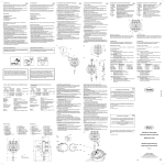
Utility files set consists of: the main file label.mth, 5 font files f_*.mth, font designer
label_fd.mth and appropriate document files *.doc. It supports plotting an arbitrary ASCII character (except graphic and control ones) or sequence of characters (text) in the 2D Plot window. Characters position, width, height, rotation (slant) and characters step in a text can be defined. Axes with
arbitrary point of their cross, numbers near ticks and labels near arrows can be plotted.
One character plotting
CHAR_(xy,wh,ch,rot) is the base function of the utility. It prepares a set of points for character ch
plotting in Options>Display>Points>Connected and Small mode. xy = [x_coordinate, y_coordinate] lower-left point of the character rectangle, and wh = [width, height] defines rectangle width and height
of this rectangle. Optional scalar parameter rot defines character rotation counterclockwise in radians.
It is zero by default. It is necessary to preload a vector font (see next paragraph) to plot characters.
CHAR_ ([1,2],[3,4],"A",0), for example, simplifies to
[[4,2], [3.5,3.5],[2.5,6],[1.5,3.5],[1,2],[1.5,3.5],[3.5,3.5]]
and gives a 3 units width and 4 units height upper case letter "A". The lower-left corner of the letter is
at the point [1,2].
D-N-L#16
p13
Sergey Biryukov: 2D Plots Labeling
Vector Fonts
Characters in the utility are divided into several groups and combined in different combinations in 5
font files: Tiny (f_t.mth) - digits, arithmetic operations and letters x, y & z; Small (f_s.mth) Tiny + English upper case letters; Small Russian (f_sr.mth) - Small + Russian upper case letters;
Full (f_f.mth) - all characters except Russian letters; and Russian Full Font (f_fr.mth) - Full +
upper & lower case Russian letters. All characters available (except Russian letters) are on Fig.1.
Each font file has two vectors: the vector of character names chars_names and the main vector chars of
the form [["character_name1", [point1, point2,..], ["char_name2",..],..]. Points are
in a standard for this font pattern rectangle. The size of this rectangle is defined in each font file.
[char_rect_width:=6, char_rect_height:=8] for all our fonts. A lot of memory space was
saved by defining character points as pairs of small integers but not rationals or decimals.
Font designer
Label_fd.mth supports new font files design by: combining data from existing font files, adding/deleting new characters to/from font files, checking fonts & character points input in the form of
long integer that reduces the number of keys to be pressed 3 times.
For example N 60533813001353 simplifies to
[[6,0],[5,3],[3,8],[1,3],[0,0],[1,3],[5,3]]
and gives an upper case letter "A" after plotting. Only nonnegative integer coordinates less than 10 can
be input with N() function and the first point can't be [0,0].
Text Plotting (Labeling)
LABEL(xy,wh,dxy,t,rot) function prepares a vector of vectors of points for plotting text t given as
vector of characters (t = ["t","e","x","t"]),
xy = [x,y] - starting point,
wh = [char_width, char_height],
dxy = [char_step_x,char_step_y],
rot - characters rotation counterclockwise in radians (optional, default=0).
Axes drawing, numbering and labeling
DRAW_AXES(xy1,xy2,axes_cross,scale_xy)
= DRAW_AXES([x1,y1],[x2,y2],[ac_x,ac_y],[sc_x,sc_y])
prepares points for drawing axes (arrows points up & right) & axes ticks in the window with the lower
- left corner coordinates xy1 = [x1,y1] & upper - right corner xy2 = [x2,y2]. axes crosses at the
point [ac_x,ac_y]. scale_xy defines distance between ticks on x & y axes. ac_x/sc_x & ac_y/sc_y
must be integers.
┌
┌ wh_x
LABEL_AXES(xy2, axes_cross, labels) = LABEL_AXES│xy2, axes_cross, │
└
└ wh_y
label_x ┐┐
││
label_y ┘┘
prepares points for labels near arrows. wh_x & wh_y are width & height of characters in x & y axes
text labels label_x & label_y.
┌┌
xy1
┐
││
│
││
xy2
│ ┌ wh_x
NUMBER_AXES(axs, numbers) = NUMBER_AXES││
│, │
││ axes_cross │ └ wh_y
││
│
└└ scale_xy ┘
┐
│
num_x ┐│
││
num_y ┘│
│
┘
p14
Biryukov: 2D Plots Labeling
D-N-L#16
prepares points for plotting num_x & num_y vectors of text under ticks.
If the tick is in the point of axes cross appropriate text is shifted left or down.
num_x = [text_for_left_tick, text_for_2nd_tick,...].
Three previous functions are combined in ALL_AXES() one that has more clear input parameters and
prepares points for plotting axes, axes labels and axes numbering. wh_x & wh_y in the second and
third arguments are different and define characters width and height for the right neighbour text.
ALL_AXES(axs, numbers, labels) =
=
┌┌
xy1
┐
││
│
││
xy2
│ ┌ wh_x
ALL_AXES││
│, │
││ axes_cross │ └ wh_y
││
│
└└ scale_xy ┘
num_x ┐ ┌ wh_x
│, │
num_y ┘ └ wh_y
┐
│
label_x ┐│
││
label_y ┘│
│
┘
Example
Don´t forget to enter all the characters under quotes, eg
numb_x ≔ ["-", "8"; "-", "6"; "-", "4"; "-", "2"; "0"; "2"; "4"; "6"]
D-N-L#16
Biryukov: 2D Plots Labeling
p15
Screenshots from original DNL#16 (December 1994)
(“DUG for YOU” and the arrows are added by me, then I tried to create a New Year´s screen, Josef)
As you can see in the following figures, Sergey´s tools are working with DERIVE 6 in the
same way.
p16
Biryukov: 2D Plots Labeling
D-N-L#16
Some Additional info about 2D Plot Labeling Utility:
1. The Utility needs DERIVE 2.04 or later
2. Its main programming ideas:
- FLOOR-function emulation. When using modern DERIVE versions, you have to exclude FLOOR
& MOD-definitions and replace TRUNC by FLOOR & A_V by APPEND.
- Strings comparison and search in a vector.
- Complex structured arguments, that simplifies using defined functions, and carries the idea of
structuring not only functions but data also.
3. There are 3 additional useful functions in LABEL.MTH not described in the paper:
APPROW(p1,p2,l) draws an arrow from point p1 to point p2 with l = arrow sides length.
BOX(p1,p2) draws a rectangle with lower left corner p1 and upper right corner p2.
SHIFT_LABEL(v,sxy) shifts a vector of broken lines v (letters or curves) by sxy = [x,y].
4. In LABEL_FD.MTH the functions INSERT_ELEMENT (v,i,a), REPLACE_EL(v,i,a) and
REPETITIONS(a,v) improves the VECTOR.MTH utility file. The first is a complementary function
to DELETE_ELEMENT(v,i). It inserts expression a in a vector v at position i. The 2nd replaces
the i-th element of v with axpression a. The 3rd returns the number of elements of vector v identical
to expression a.
Conclusion
Utility described can be easily used on every IBM PC compatible computer. Only 2 files are to be
loaded as utilities: label.mth & one of the font files (*.mth). Only 2 functions are needed by the
user: LABEL() - for writing graph labels & ALL_AXES() for axes drawing, labeling and numbering.
Full Fonts are rather slow on IBM PC/XT, so, Tiny & Small Fonts for these computers are highly recommended.
Acknowledgments
My thanks to Dr. B. Kutzler for the idea of writing this paper, V.B.Biryukov for draft fonts design &
Prof. N.V.Soina for friendly advices and support.
Comments of the editor:
I do neither list LABEL.MTH nor LABEL_FD.MTH, you can download the files from the subdirectory <LABEL>. Included are many files with font sets. I am adding here the most important
names which are packed in separated mth-files (which must be preloaded before using). I
had to change some 1994-files because the DOS-characters are not compatible with the
Unicode-characters of DERIVE 6 – and it might be too complicated to include them now. This
is the reason that I copy some screens with the respective characters.
f_e.mth: English Upper case and Lower case letters
f_el.mth: English Lower case letters
f_eu.mth: English Upper case letters
f_gr.mth: ["α","ß","Γ","δ","ε","Θ","µ","π","σ","τ","Φ","Ω","∩","Σ",
"gamma_low","fi_low","omega_low","delta_up"]
D-N-L#16
Biryukov: 2D Plots Labeling
p17
See first the font sets from 1994 and then the changed sets adapted for DERIVE 6.
f_mef.mth: ["∞","φ","ε","∩","≡","±","≥","≤","⌠","⌡","÷","≈"]
f_mf2.mth: ["°","·","·","√","ⁿ","²","■"]
f_mfr.mth: ["≥","≤","⌠","⌡","÷","≈","°","·","·","√","ⁿ","²","■"]
f_n0.mth: ["#","$","@","[","\","]","^","`","{","|","}","~"]
The next sets are still valid.
f_s.mth: ["!","double_quotes","%","&","'","(",")","*","+",",","-",".","/",
"0","1","2","3","4","5","6","7","8","9",":",";","<","=",">","?","_",
"A","B","C","D","E","F","G","H","I","J","K","L","M","N","O","P","Q",
"R","S","T","U","V","W","X","Y","Z"]
f_t.mth:["!","double_quotes","%","&","'","(",")","*","+",",","-",".","/",
"0","1","2","3","4","5","6","7","8","9",":",";","<","=",">","?",
"_","X","Y","Z"]
It is important that the two lists (vectors) forming the font-set-mth-file are called char_names
(the short one) and chars (the huge one). Have a look at this vector and admire the enormous work lying in them. Maybe you will create another font set for us!! Editor.
p18
Heinz Rainer Geyer: Der Fermat-Punkt
D-N-L#16
Der Fermat-Punkt im Dreieck
The Fermat-Point in the Triangle
H.R.Geyer, Wiesbaden, GER
Während einer Projektwoche an unserer Schule (Gymnasium) im Frühjahr 1993
beschäftigte sich eine Gruppe von 7 Schülern der Jahrgänge 9 bis 13 mit den
Einsatzmöglichkeiten von DERIVE im Mathematikunterricht. Bis auf einen Schüler hatten sie keine Erfahrungen mit dem Programm. Nach dem Einführungstag
(4 Schulstunden) hatten sich alle soweit in die Bedienung eingearbeitet, dass sie in
der Lage waren, sich an aktuellen Problemen des Mathematikunterichts der jeweiligen Jahrgangsstufe zu versuchen.
Am 3. Tag stellte ich allen gemeinsam eine Aufgabe:
Es ist die Lage desjenigen Punktes in einem (spitzwinkeligen) Dreieck zu suchen,
dessen Abstandssumme zu den drei Eckpunkten minimal ist - der Fermat - Punkt.
During a project week at our school (grammar school) in spring 1993 a group of 7 students
(age 15 - 19) dealt with DERIVE. After a short introduction - 4 hours - they were able to use
DERIVE in connection with actual problems of their curriculum. On the 3rd day I set them all
the same task:
Find the point in an acute triangle ABC with a minimal sum of distances to the points
ABC - the Fermat point. To explain the problem I showed the following proof by construction:)
Zur Erklärung führte ich den folgenden geometrischen Konstruktionsbeweis vor:
Sei T zunächst ein beliebiger Punkt im
Dreieck ∆ABC. Dreht man das Teildreieck ∆CAT um 60° in positiver Drehrichtung um den Punkt A, so ergibt sich ein
Polygonzug C´T´TB, dessen Länge die
gesuchte Abstandssumme ist. Die Länge
des Polygonzuges ist minimal, wenn er
auf der Geraden C´B liegt.
Analog dreht man das Teildreieck ∆TBC
um B um –60°. Der gesuchte FermatPunkt F ergibt sich also als Schnittpunkt
der beiden Geraden C´B und C´´A.
This is the original screen shot from 1994. The labels were
produced using Sergey Biryukov´s labeling tool.
T is an arbitrary point in ∆ABC. Having rotated ∆CAT about 60° in positive direction you obtain the sum of the distances with the polygon C´T´TB. Ist length is minmal, if it coincides
with the line C´B. In the same way you can rotate ∆TBC round B by –60° (negative). The
Fermat - point is the intersection point of C´B with C´´A.
It was interesting to observe how the pupils found different ways to solve the problem according to their mathematics knowledge.
D-N-L#16
Heinz Rainer Geyer: Der Fermat-Punkt
p19
We can use dynamic geometry to illustrate the problem and to verify that interection point FP
is indeed the solution point:
I show the Cabri-figure (PC and TI-92/Voyage 200) and the TI-Nspire-figure(s), Josef.
Zur analytischen Bestimmung von F wurde vereinbart, das Dreieck in einem kartesischen Koordinatensystem mit A(0/0) zu beschreiben.
Die Schüler kamen nun selbständig je nach Kenntnisstand auf folgende Lösungsansätze:
I. Berechnung des numerischen Abstandswertes als Funktion des Punktes F(x,y) und
Minimieren durch sukzessive Einengung der Definitionsbereiche für x und y
Calculation of the numerical value as a function of the point F(x,y) and minimization by a
step by step restriction of the domains for x and y
Definition of the TOTAL sum of distances:
#1:
#2:
[b1≔,b2≔, c1≔,c2≔]
2 2
da(x,y) ≔ √(x +y )
#4:
2
2
db(x,y,b1,b2) ≔ √((x-b1) +(y - b2) )
2
2
dc(x,y,c1,c2) ≔ √((x-c1) +(y-c2) )
#5:
TOTAL(x,y,b1,b2,c1,c2) ≔ da(x,y)+db(x,y,b1,b2)+dc(x,y,c1,c2)
#3:
p20
D-N-L#16
Heinz Rainer Geyer: Der Fermat-Punkt
Substitution of the co-ordinates of the given vertices of the triangle:
#6:
L(x, y) ≔ TOTAL(x, y, 7, 2, 3, 5)
It follows an evaluation of function L in a 5 x 5 matrix,
with increment h starting with x = s and y = t:
#7:
FERM(s, t, h) ≔ VECTOR(VECTOR(L(x, y), x, s, s + 4·h, h), y, t, t
+ 4·h, h)
#8:
FERM(3.41, 3.12, 0.002)
#9:









10.30679813
10.30679185
10.30678803
10.30678668
10.30679055
10.30678457
10.30678106
10.30678002
10.3067845
10.30677882
10.30677562
10.3067749
10.30677998
10.30677461
10.30677173
10.30677131
10.306777
10.30677194
10.30676936
10.30676927
#10:
FERM(3.415, 3.127, 0.001)
#11:









10.30676992
10.3067701
10.3067709
10.30677232
10.30676901
10.30676927
10.30677015
10.30677165
10.30676848
10.30676882
10.30676978
10.30677136
10.30676834
10.30676876
10.3067698
10.30677146
10.30676858
10.30676908
10.3067702
10.30677194
10.3067878


1.30678146 

10.30677665 

10.30677338 

10.30677165 
10.30677436 

10.30677377 

10.30677356 

10.30677373 

10.3067743 
Value of the distance-sum-function:
#12:
L(3.415, 3.13) = 10.30676834
Die beiden Beispiele aus dem DERIVE-Programm zeigen, daß die Auswertung der Matrizen zwar
schwierig - weil unübersichtlich - ist, aber die Lage des Fermat-Punktes läßt sich so doch gut einengen.
Both examples show that the evaluation of the matrices is difficult because not easy to survey, but we can find the position of the Fermat point approximatively.
The numerical approach would be easier to follow if we could include the x- and y-values as well in the
table. This is possible with little manipulating the matrix – and the respective function could be provided as a tool by the teacher.
Producing a table including the x- and y-values:
#13:
values(s,t,h) ≔ APPEND([APPEND([],VECTOR(y,y,t,t+4h,h))],FERM(s,t,h)`)`
#14:
values(3.41, 3.12, 0.002)
#15:











3.41
3.412
3.414
3.416
3.418
3.12
10.30679813
10.30679185
10.30678803
10.30678668
10.3067878
3.122
10.30679055
10.30678457
10.30678106
10.30678002
10.30678146
3.124
10.3067845
10.30677882
10.30677562
10.3067749
10.30678146
3.126
10.30677998
10.30677461
10.30677173
10.30677131
10.30677338
3.128
10.306777
10.30677194
10.30676936
10.30676927
10.30677165
Then proceed as shown above.











D-N-L#16
Heinz Rainer Geyer: Der Fermat-Punkt
p21
II. Differentiation der Abstandssummenfunktion
(Differentiation of the distance-sum-function)
Für die Schüler der Klasse 11 lag es nahe, den Extrempunkt der Abstandssummenfunktion L(x,y) über
die Ableitung zu suchen. Als Funktion zweier Veränderlicher entzieht sie sich allerdings dem für
Schüler bekannten Lösungsverfahren. Einer der Schüler hatte hier die Idee, die partiellen Ableitungen
von L(x,y) als Funktion der einen Variablen bei konstantem Wert der zweiten Variablen zu plotten.
Hierzu definierte er einen Vektor, dessen Komponenten jeweils die so bestimmten partiellen Ableitungen waren. Die dargestellten Graphen führen zwar nicht direkt zu den Koordinaten des gesuchten
Punktes, zeigen aber „auffälliges“ Verhalten in der Nähe der Koordinaten des Fermat–Punktes und
insbesondere an den Grenzen der durch die Dreieckspunkte bestimmten Definitionsbereiche.
The pupils of form 11 tried to find the extremal pont of the distance sum function using the derivative.
Being a function of two variables it exceeds the pupils´ known algorithms. One of the students had the
idea to plot the partial derivatives of L(x,y) wrt one variable keeping the other one constant. The
graphs don´t lead directly to the point we are looking for, but they are showing a very “strange“ behaviour in the neighbourhood of the point and especially at the borders of the domain defined by the angles of the given triangle.
Original figures from DNL#16 (DOS-Derive)
Caution: The earlier Derive versions were
not able to plot implicit functions, and they
accepted all variables as the independent
variable. Now we can do implicit plots and
the graph of the 2nd family has another appearance:
p22
Heinz Rainer Geyer: Der Fermat-Punkt
D-N-L#16
II. Nachbildung des geometrischen Beweises als Schnittproblem zweier Geraden
(Reproducing the geometric proof as intersection point of two lines)
Hierzu mußten die Koordinaten der gedrehten Punkte C´ und C″ bestimmt werden. Die Schüler experimentierten dazu zunächst mit Tangens und Pythagoras. Zur Vereinfachung wurden dann die erforderlichen Drehungen nur auf Drehungen um den Ursprung (Punkt A) beschränkt. Außerdem stellte ich
den Schülern die Matrix einer Drehung um den Ursprung und ihre Anwendung auf Ortsvektoren sozusagen als “Black Box-Funktion“ zur Verfügung. Entscheidend war, dass die Koordinaten der gedrehten Punkte C_ und B_ zur Verfügung standen.
Damit konnten die Geradengleichungen aufgestellt werden und das Schnittproblem auf dem Niveau
der Klasse 9 gelöst werden.
The co-ordinates of the roteted points C´and C“ were necessary. At first the students experimented with Tangens and Pythagoras. As a simplification I made the rotation matrix available to the students - as a Black Box. Having the points C´and B´ the problem was easy to
solve for pupils even of level form 9.
D-N-L#16
Heinz Rainer Geyer: Der Fermat-Punkt
p23
We repeat the calculation for the Nspire-Triangle from page 19:
The Cabri-plot with the rotated triangle ATB (which is used for the proof)
Die Darstellungen zeigen deutlich, daß das Problem sicher nicht abschließend behandelt wurde. Es
gibt noch viele Möglichkeiten zur Verfeinerung, zB beim Problem der Ableitungen oder bei der
Schnittpunktsberechnung. Ich hoffe aber, daß deutlich wurde, wie ergiebig dieses Fermat-Problem für
den Mathematikunterricht in vielen Klassenstufen ist und wie hervorragend sich dabei ein Programm
wie DERIVE einsetzen läßt. Der experimentelle Charakter der mathematischen Arbeit in unserem
Projekt bewirkte jedenfalls einen erkennbaren Motivationsschub, der dem Mathematikunterricht insgesamt bestimmt zu gute kommt.
(The presentations are showing very clear, that we couldn´t deal with the problem sufficiently. There are many possibilities for refinement. But I hope that I could show how productive this problem could be for many forms and how excellent you can use DERIVE for this
purpose. The experimental character of the mathematical work in our project caused a significant motivation which could be very useful for maths teaching in total.)
Additional comments for the revised version of DNL#16 will follow on the next page:
p24
Heinz Rainer Geyer: Der Fermat-Punkt
D-N-L#16
The students had the idea of applying calculus. So one could provide the suggestion to equate both
partial derivatives to zero and … then try to solve the resulting system of equations:
Inspecting the partial derivaties might discourage the students from solving the system. But they might
also have heard or even learned to apply the Newton-Raphson-algorithm for approximatively solving
equations. Why not extend for more variables??
Using the DERIVE-Help they might find NEWTONS(u, x, x0).
Here we see the last three iterations of the algorithm.
And finally it might be a welcome surprise to show the solution in a 3D-environment.
L(x,y) from expression #6 is a function of two variables which can be plotted immediately in the
3D-Plot window. The students have to find appropriate settings for the box.
Using the Trace tool they are asked to find the “Minimum Point” and then they can add the point
(xFP, yFP, L(xFP, yFP)).
D-N-L#16
Thomas Weth: A Lexicon of Curves
(5)
p25
Ebene Algebraische und
Transzendente Kurven
(5)
Thomas Weth, Würzburg, Germany
Die Hundekurve - Die Konchoide des Nikomedes
Die in dieser Folge behandelten Kurven sind Erweiterungen
der sog. „Hundekurve“ oder „Tractrices“. Tractrices entstehen, wenn ein Herrchen seinen Hund auf einem geraden Weg
führt, während der Hund - bei konstanter Leinenlänge - seinem „Lieblingsbaum“ zustrebt. Mathematisch formuliert
handelt es sich bei dem Weg des Hundes um eine spezielle
Form von Konchoiden.
The curves dealt with in in this sequel are extension of the
so called “Dog´s curve“ or “Tractrices“. They are created
when a man walks along a line while his dog - kept on a lead
with constant length - wants to visit his favourite tree. From
the mathematical point of view the dog´s way is a special
form of a conchoid.)
Erzeugung von Konchoiden - How to create a conchoid
Konchoiden im allgemeinen ergeben sich nach folgender
Konstruktionsvorschrift:
Gegeben ist eine ebene Kurve C und ein Punkt O in ihrer
Ebene. Von einem Punkt Q der Kurve aus trägt man auf der
Geraden OQ in die beiden möglichen Richtungen jeweils
eine Strecke konstanter Länge K ab; die Endpunkte P1 und
P2 dieser Strecken sind dann Konchoidenpunkte zur Kurve
C.
This is the instruction how to obtain a conchoid: given is a plane curve and a point O in its plane. Have
any point Q∈C. The two points P1 and P2 on the line OQ with QP1 = QP2’ = K (const) are points of a
conchoid to C. If the curve C is a line the conchoids are especially simple, they are tractrices. Nikomedes (200 BC) invented this curve for doubling a die and for trisecting an angle. Its name is derived
from the greek word for shell: κóγχη.)
Die Konchoide des Nikomedes - Herleitung der algebraischen Kurvengleichung
Besonders einfache Konchoiden ergeben sich, wenn die Leitkurve C eine Gerade ist (wie im Beispiel
der Tractrix). Diese Kurven wurden von Nikomedes (ca 200 v.Chr.) zur Würfelverdoppelung und zur
Dreiteilung des Winkels erfunden. Der Name ist wegen der Kurvenform abgeleitet vom griechischen
κóγχη, Muschel.
Für die Kurvenpunkte P1/2 ergibt sich in Polarform (vgl. obige Zeichnung):
Thomas Weth: A Lexicon of Curves
p26
P1,2 : r =

a
cos ϕ
± K oder  r −

(5)
D-N-L#16
a 
 ∓ K = 0 und daraus für die gesamte Kurve:
cos ϕ 
2
a
a
a 




2
 r − cos ϕ − K   r − cos ϕ + K  = 0 oder kurz  r − cos ϕ  = K .





(Polargleichung der Konchoide des Nikomedes; this is the polar form of Nikomedes´ conchoid. Now you easily can find the Cartesian form:)
Den Übergang zu kartesischen Koordinaten erhält man mit x = r cos(ϕ) und y = r sin(ϕ):
2
 a⋅r 
2
2
2
2
r −
 = K . Ersetzt man nun noch r = x + y (DERIVE!) und faktorisiert die Summe, so
x 

erhält man die algebraische Kurvengleichung
(x
2
+ y2 )( x − a ) = K 2 x2.
2
Aus der Kurvengleichung läßt sich nun entnehmen, dass die Kurven (für verschiedene K)
• symmetrisch zur x-Achse sind,
• die Leitgerade C mit der Gleichung x = a zur Asymptote haben und
• im Ursprung einen (evtl isolierter) Kurvenpunkten haben.
(From the curve´s equation you can see that for different values for K, the curves
•
•
•
are symmetric in respect to the x-axis,
have line C with x =a as an asymptote and
the origin is a (eventually isolated) point of the curve.)
Für die Fälle K < a, K = a und K > a ergeben sich die drei Kurvenformen:
K<a
K=a
K>a
DERIVE 6 has two remarkable features which we can use to reproduce the construction of
this curve: the slider bars and the possibility to switch between rectangle coordinates and
polar coordinates in one session. This one more occasion to narrow the gap between computer algebra and dynamic geometry. I´ll try to explain the procedure very briefly guided by
the following screen shots, Josef
D-N-L#16
Thomas Weth: A Lexicon of Curves
This is the “Dog´s curve” on the hand held TI-Nspire.
(5)
p27
p28
Thomas Weth: A Lexicon of Curves
(5)
D-N-L#16
Verwendung der Konchoide zur Würfelverdoppelung - Doubling a die
Zu konstruieren ist die Kantenlänge x eines Würfels, der den doppelten Inhalt besitzt wie ein Würfel
mit der Kantenlänge a; also x3 = 2 a3 oder x = a 3 √2.
Dazu zeichnet man eine Konchoide mit K = a und
zeichnet durch U unter 60° eine Gerade zur xAchse, die den rechten Kurvenzweig in S schneidet. Die Gerade OS schneidet die Leitkurve C dann
im Punkt T. x = OT ist dann die gesuchte Würfelkante mit x3 = = 2 a3.
OT = x is the edge of the cube with x3 = 2 a3.
Nach dem Strahlenlsatz ist nämlich
x : a = 2a : y bzw x ⋅ y = 2a2 . (I)
Mit dem Lot von O auf die Gerade US ist das
Dreieck OSL rechtwinkelig und es gilt zunächst:
LU = a cos (60°) = a .
2
Damit folgt für das Dreieck ∆OSL:
2
2
( x + a) =  y + a2  + OL


2
2
2
und für das Dreieck ∆OLU: a2 = a + OL .
4
2
2
2
2
2
Subtraktion liefert: ( x + a) − a2 =  y + a  − a bzw. x + 2 a x = y + a y
2
4

(I) und (II) vereinfacht man durch Elimination von y zu x3 = 2 a3.
You can simplify (I) and (II) by eliminating y and you obtain x3 = 2a3
Verwendung der Konchoide zur Drittelung des Winkels
How to use the conchoid to trisect an angle
Ist α der zu drittelnde Winkel, so trägt man auf dem einen Schenkel eine beliebige Strecke [OU] mit
der Länge a ab. Das Lot in U auf die Gerade OU schneidet den anderen Schenkel im Punkt N.
Mit ON = c zeichnet man zur Leitgeraden NU eine Konchoide mit O als Pol und K = 2c. Durch N
zeichnet man die Parallele zu OU, welche die Konchoide im Punkt P trifft. Dann ist: ∠POU
=
α
3
.
D-N-L#16
Thomas Weth: A Lexicon of Curves
(5)
p29
If you want to trisect α, then take any arbitrary point U with OU = a on one side. The perpendicular intersects the other side of α in N. With ON = c draw a conchoid with respect to the
line NU with O as ist pole and K = 2c. Let NP ║ OU , then ∠POU is the third of ∠NOU
Begründung:
Ist M die Mitte von QP, so liegen P, Q und N auf dem Thaleskreis über der Strecke [PQ]. Also ist
PM = MQ = MN = c = ON. Damit gilt:
∠ NPM  = ∠ MOU  = ß
(als „Z - Winkel“).
Da das Dreieck MPN gleichschenkelig ist, gilt für den Außenwinkel ∠OMN:
∠ OMN = 2 β .
Da außerdem das Dreieck OMN gleichschenkelig ist, gilt wegen der Kongruenz der Basiswinkel:
(M is in the middle of PQ, then P, Q and N are lying on a Thales circle, so PM = MQ = MN =
c = ON.
Then you will find two isosceles triangles ∆MPN and OMN∆, giving simple relations between
the angles.)
∠ MON = ∠ OMN = 2 β . also ist α = 2 ß + ß oder ß = α/3.
Es sei hier ausdrücklich darauf hingewiesen, daß es sich bei den Konstruktionen zur Würfelverdoppelung und zur Winkeldreiteilung nicht um elementare Zirkel- und Linealkonstruktionen im Platon´schen Sinne handelt. Wie man an den vorhergehenden Beispielen sieht, ist nämlich die Würfelverdoppelung und die Winkeldreiteilung sehr wohl geometrisch möglich - nur eben nicht - wie zB in der
Galois-Theorie bewiesen wird - mit Zirkel und Lineal alleine. In den obigen Konstruktionen wurde
nämlich eine Gerade mit einer Kurve (der Konchoide) geschnitten, also eine Operation durchgeführt,
die mit Zirkel und Lineal alleine nicht möglich ist.
Abschließend sei bemerkt, dass sich für einen Kreis als Leitlinie andere bekannte Konchoiden, u.a. die
Pascalschen Schnecken und die Kardioide ergeben. Wir werden in einer späteren Folge darauf zu
sprechen kommen.
I want to emphasize that these constructions are not elementary constructions using ruler
and compasses only in Platon´s sense, because you need the intersection point between a
conchoide and a line and this operation can´t be done with the tools mentioned. The Galois
Theory proofs this fact.
Finally I would like to mention, that using a circle as leading line we will find other well known
conchoids as Pascal´s snail and the cardiode. In a later sequel we will talk about.
p30
J.C.M. Verhoosel: T-periodic Functions
D-N-L#16
DERIVE and plotting
T - periodic functions
Drs.J.C.M.Verhoosel, Eindhoven, Netherland
Introduction.
For most simple periodic functions it is rather easy to plot them. Think of y = sin(x) for instance. Just
Author sin(x), press twice on Plot and voila.
It is more difficult to plot functions like those in figure 1.
Figure 1: “difficult“ periodic function.
We will discuss the possibilities and problems connected with plotting this kind of functions.
The tools.
Derive knows the following functions:
a) CHI(a,x,b); a function which returns 1 for x ∈ [a,b] and 0 outside [a,b]
b) The IF - function. We can use this function for piecewise definded expressions using conditions.
For instance: IF(x < 0, x2,, x) is a function which for x < 0 returns a parabola and for x ≥ 0
the straight line y = x.
c) MOD(a,b) which approximates to a modulo b. When MOD(x,1) is plotted, you get a sawshaped-function. MOD(x,π) also returns a saw shaped function but now with period π.
d) FLOOR(x) is narrowly connected to MOD(x). Simplifying MOD(x,1) yields x - FLOOR(x).
In other words: MOD(x,1) = x - FLOOR(x).
Plotting using CHI, IF and MOD
The usage of CHI.
Let´s look at the following piecewise defined function:
f(x) = x2 if x ∈ [0,1] and 0 if x ∉ [0,1]
We could Author this with: f(x) := CHI(0,x,1) x2.
A short explanation:
The fact that the product is forced to 0 outside [0,1] makes it rather difficult for us to plot functions
only defined on an interval: DERIVE plots 0 outside the interval while the function is not defined over
there.
D-N-L#16
J.C.M. Verhoosel: T-periodic Functions
p31
Let´s suppose we want a function like the one in figure 1. We can define f(x) on [0,1], on [1,2] etc. The
next step is to define this function in terms of SUM: Apparently it´s not a problem when the number
of terms is finite.
On [0,1] we get 4 CHI(0,x,1) (x - 0.5)^2.
The quadratic function defined on [1,2] would be f(x) := 4 CHI(1,x,2) (x – 1.5)^2;
the one on [k, k+1]: 4 CHI(k,x,k+1) (x – 0.5–k)^2.
So when we take the first 5 terms we get:
5
f ( x) := ∑ 4 CHI(k , x, k + 1) ( x − 0.5 − k )2
k =0
This function isn´t a true periodic function. To produce a true periodic function f(x) must become
symmetric and extended to infinity (and negative infinity). So let us define g(x):
g ( x) :=
∞
∑
4 CHI(k , x, k + 1) ( x − 0.5 − k )2
k =−∞
Although DERIVE is capable of plotting f(x), it accepts g(x) but seems not capable of plotting it.
Probably DERIVE tries to evaluate the function and can´t handle infinity.
Using IF
What about the IF - function? We can use this function to make a piecewise defined function: for instance: f(x) := IF(x < 0 OR x > 1,x,x2).
A short explanation:
When x < 0 or x > 1, then f(x) = x, everywhere else f(x) = x2.
Another example: g(x) := IF(x < -1 AND x < 2,x,?)
When we plot g(x) we can see that outside [-1,2] g(x) is not forced to 0 because the function is not
defined there.
Nevertheless we have the same problems with the “IF - command“ as those we encountered with the
CHI-functions: it is not possible to plot true piecewise defined functions although it is possible to define them!
Using MOD(a,b)
Because MOD(x,a) already is a periodic function, it offers more perspectives. Moreover, it is not
necessary for a to be an integer: for instance MOD(5,2.1) will yield 0.8.
For students this function often gives surprises. It´s not automatically clear for them why the plot of
x MOD(x) or MOD(x^2) looks so strange. These plots invite the students to discuss simplifications
in DERIVE involving MOD(x). Can we understand what is happening here? What is the connection
between FLOOR(x) and MOD(x)? After some experimenting in DERIVE they find it rather easy to
understand that MOD(x) = x - FLOOR(x) and x MOD(x) simplifies to x^2 - x FLOOR(x).
p32
J.C.M. Verhoosel: T-periodic Functions
D-N-L#16
Figure 2
The usage of MOD(x) in plotting periodic functions.
To understand how MOD(x,y) can be used to plot T-periodic functions, we must understand how
MOD(x,y) works (see window 4 of figure 2 for a plot of MOD(x)).
MOD(x) can be used to make sure that for instance f(3.2) will be reduced to f(0.2). This means that f(x)
can be 1-periodic: the part on the domain [0,1] is repeated.
MOD(x) can be used to draw other, random composed, periodic functions. MOD(x) has period 1:
every x is reduced to a value between 0 and 1. Replacing x with MOD(x) gives us a 1-periodic function!
A nice way to create a T-periodic functions is to transform the function defined on [0,1] by multiplication / translation etc.
An example:
We want a “periodic parabola“ through the points (0,1) and (1,1) which is symmetrical on the axes
x = 0.5. (see figure 3).
Figure 3: the quadratic curve.
D-N-L#16
J.C.M. Verhoosel: T-periodic Functions
p33
First we must find the formula of the quadratic curve: f(x) := 4 (x – 0.5)2. This function surely is defined on [0,1]. Now we replace x by MOD(x) which gives us the function
f(x) := 4 (MOD(x) – 0.5)2. Plot the formula and you get figure 4.
Figure 4: 2-periodic quadratic curve.
Suppose we want to translate this function so that the minimum of the quadratic curve occurs for
x = 0, then we must replace x by x – 0.5. In the same way we can get a 2-periodic function by replacing x by x/2 etc.
Another example:
We want a series of half-circles. At first you can define a half circle on [0,1] (see figure 5). Solving for
y gives us 2 possibilities, we choose the positive one.
The only thing we must do now is to replace x by MOD(x). In the same way we get a 2-periodic series
by replacing x by x/2. The period is twice as big but not the amplitude. So we´ll have to multiply our
function as well by a factor 2. Now we have a true 2-periodic series of half-circles.
Figure 5: a series of half-circles
(It is interesting that DERIVE “simplifies” the functions, when we have them annotated in the
plot window! Josef)
Noting that MOD(x,2) already has a period 2, it must be possible to do things more easy.
Suppose we plot y = x 1 − x .
p34
J.C.M. Verhoosel: T-periodic Functions
D-N-L#16
Suppose we plot y = x 1 − x .
To make sure that the next period is produced we must be sure that x = 2.1 for instance is reduced to
x = 0.1. This can be done by MOD(x,2). So we replace x by MOD(x,2) and get:
y =
MOD ( x, 2)
1 − MOD ( x, 2) .
When we plot this function we get 2-periodic function in the next figure.
Let´s try this on another function. Suppose f(x) is defined as:
f(x) = x2 when x ∈ [-0.2, 0.4] and 0.6 - periodic.
We are tempted to replace x by MOD(x,0.6). Why does this not work?
Looking at x = 0.7 we see that MOD(x,0.6) reduces it to 0.1 while it should be reduced to -0.1. We
have to transform MOD(x). The period is all right: 0.6. The starting point is not correct. It should
be –0.2, so: will MOD(x + 0.2,0.6) work? Not yet. Suppose we look again at x = 0.7. Now it is reduced to MOD(0.7 + 0.3,0.6) = 0.3, still not correct. We must realize that we should subtract 0.2, so it
should be: MOD(x + 0.2,0.6) – 0.2!!!
We can generalize this to the procedure shown in the next figure:
Combining ....
There is no restriction on the form of the function
which is to be made periodic. We can join x2 on
[–0.2,0.4] with 0.56 – x on [0.4,0.6] for instance.
In this case we make use of the IF- or CHIfunction:
D-N-L#16
J.C.M. Verhoosel: T-periodic Functions
p35
We can generalize this to the procedure shown in the next figure:
This works also with an IF-construction instead of the CHI-function for the piecewise defined
function. Josef
How to automate the process.
In lectures on Fourier analysis students construct a function f(t) by summing harmonics.
When the original function is T-periodic, they can match it with their own constructed function. To avoid unnecessary arithmetic one could automate the process by defining the next
function:
From now on it´s rather easy to use.
p36
J.C.M. Verhoosel: T-periodic Functions
D-N-L#16
We have now the possibility to compare a Fourier - approximation of f(x) with f(x) itself, as
you can see below!
Conclusion.
DERIVE can be a useful tool for plotting T-periodic functions. Although it is possible to define and
use T-periodic functions with CHI and SUM they can´t be plotted. The use of MOD(x,T) is simpler
and more elegant. Nevertheless, the process of defining true T-periodic functions with CHI and SUM
and the use of transformations is very learningful. The use of PERIODIC( ) appears to be very useful
in the classroom.
D-N-L#16 J.M.C. Lopes: Ill - Conditioned Problems
p37
DERIVE, Newton Method and
Ill - Conditioned Problems
Jose M.Cardia Lopes, Porto, Portugal
J. Böhm (1993) has recently written in this magazine about the Newton method for
solving non linear equations pointing out, by means of an interesting example, the
crucial importance of the choice of the initial values. The popularity of this method is
due mostly to its quadratic convergence if the initial values are well chosen. (If it
doesn´t converge the divergence soon becomes obvious.) Nevertheless with illconditioned problems the Newton method (as any method ...) can lead to a large
number of iterations and to not very good solutions.
A particular class off ill-conditioned problems which often appear in the classroom is the problem of solving polynomial equations with multiple roots. In fact it can be demonstrated that if we have
an equation f(x) = 0 with a multiple root X, if f p(x) is the computer representation of f(x) (with the
“perturbations” due to the ill-condition), if ∆ is an upper bound on the perturbations in f(x), and if Xp is
the corresponding root of f p(x) = 0, then
1
m

m! 
X − X ≈  (∆

m)

 f (X ) 
p
where m is the multiplicity of the root. With this expression we can evaluate the effect of a perturbation in f(x) on the determination of the multiple root of the equation. As a result of the power 1/m the
determination of multiple roots may be an ill-conditioned problem.
Since the ill-conditioning is a consequence of the problem structure, we can only avoid it if we
change the problem structure. For a polynomial equation we can substitute the evaluation of the multiple root of
f ( x) = 0
by the evaluation of the single root of
u( x ) = 0
where
u ( x) =
f ( x)
f ′( x)
(see for example, Chapra e Canale, 1990).
This is another situation in which DERIVE can be a very good pedagogical tool. We can
graphically show how the structural change of the problem improves dramatically the path to the root.
We can see some examples:
Example 1:
f ( x) = ( x − 3)6 (2 x − 5)
Derive has no difficulty to solve this equation but the graphical representation suggests that the Newton method converges on the multiple root x = 3 at a very slow rate (notice that the function does not
cross the x-axis at x = 3). The situation is very different with u(x).
p38
Example 2:
J.M.C. Lopes: Ill - Conditioned Problems
D-N-L#16
f ( x) = (5 x − 14)2 ( x2 + 3)
If the lecture is designed for beginners there will probably be some interest in a more detailed
approach (like the one prposed by Dyer (1993)) to show the results of some interations.
In addition the second example points out the importance of the manipulation of the mathematical expressions in order to minimize the number of arithmetic operations. See the plots of the factorized and the expanded function.
(There is no difference now in higher versions of DERIVE, Josef)
Screen Shot from the 1994 DERIVE for DOS version
References
Böhm J. (1993) “Newton-Raphson´s Chaos”, The DERIVE Newsletter #12, p 10 -13
Chapra, S.C & Canale, R.P. (1990), “Numerical Methods for Engineeers”, 2nd ed, Mc-Graw-Hill
Dyer, D. (1993) “The Bisection Method and DERIVE”, The DERIVE Newsletter #11, p 11-13
D-N-L#16
Keith Eames: Functions Transformations
p39
Find here a worksheet of Keith Eames:
Exercise
Use the graphical capability of Derive to answer these questions. Check your answers agebraically using Derive.
Explain how you can get form F(x), by a single transformation whenever possible, to each
G(x) in all of the following questions:
1. Draw the graph of F(x) = x2 - 2x + 3.
a) G(x) = x2 + 2x + 3
b) G(x) = - x2 + 2x - 3
c) G(x) = - x2 - 2x - 3
d) G(x) = x2 + 4x + 6
e) G(x) = 3x2 - 6x + 9
c) G(x) = 4x2 - 4x + 3
2. Draw the graph of F(x) = (2x - 1) (3x + 5)
a) G(x) = 6x2 + 7x + 4
b) G(x) = 6x2 - 7x - 5
c) G(x) = 6x2 - 29x - 28
d) G(x) = 10 - 14x - 12x2
e) G(x) = 54x2 - 21x - 5
f) G(x) = 6x2 + 31x + 28
3. Draw the graph of F(x) = 2x3 - 3x2 - 9x + 10
a) G(x) = 2x3 - 3x2 - 9x
b) G(x) = 2x3 - 9x2 + 3x + 14
c) G(x) = - 4x3 + 6x2 + 18x - 20
d) G(x) = 10 + 18x - 12x2 - 16x3
e) G(x) = 2x3 + 9x2 + 3x
f) G(x) = 16x3 - 12x2 - 18x - 10
4. Draw the graph of F(x) = sin (x)
3
1
sin( x ) + cos( x )
2
2
a) G(x) = 2 sin(x) cos(x)
b) G(x) =
c) G(x) = cos
d) G ( x ) = 2 sin( x ) −
e) G(x) = sin(x) + cos(x)
f) G(x) = 1 + 3 sin(x) - 4 sin 3 x
2 cos( x )
All the trig functions in the above are in radians not degrees
Hint: Use the well known fractional multiples of π
5. Is it always possible to map a quadratic function to another quadratic function by a series of
transformations? Experiment with your own quadratic equations. Can you prove any of
your findings? Give some examples! What is the maximum number of different single
transformations that is required?
p40
Keith Eames: Functions Transformations
D-N-L#16
Answers
1. Use a trial and error method to find possible answers.
Simplify F(x+1)
Compare the given answers with G(x)
a) F(-x)
b) -F(x)
c) - F(-x)
d) F(x+3)
e) 3 F(x)
f) F(2x)
2. If Derive does not give the answer shown Expand the expressions and compare.
a) F(x)+9
b) F(-x)
c) F(x-3)
d) - 2 F(x)
e) F(- 3x)
f) F(x+2)-5
b) F(x-1)
c) - 2 F(x)
d) F(-2x)
e) F(x+2)+4
f) F(2x)-20
b) F(x + π/6)
c) F(2x)
d) 2 F(x - π/4) e) √2F(x + π/4) f) F(3x) + 1
3.
a) F(x) - 10
4.
a) F(2x)
5. F(x) = ax2 + bx + c can be transformed to G(x) = rx2 + sx + t by at most 4 transformations,
this depends on the values of a and r.
If r and a are both positive then ist 3 transformations:
 r 
b
s 
s2
b2
F
x
−
+
t
c
+
−
−
+


2 r 
4r
4a
2 r a
 a
How does this formula change if a is positive and r is negative?
When you have finished this assignment and you are happy if your results and conclusions
ask for the next worksheet.
Answer the questions on it without using Derive.
A correction: In the last DNL I published H. Scheuermann´s phone number. One digit
was wrong, this is the right number: 06192 27568
Please don´t forget to renew your subscription for 1995 in time. Administration would be
much easier for us. If you don´t cancel then we assume that you will stay a member. Many
thanks for your cooperation.
Bitte denken Sie daran, rechtzeitig Ihre Mitgliedschaft zu erneuern. Falls Sie nicht kündigen, dürfen wir annehmen, dass Sie Mitglied bleiben. Herzlichen Dank für Ihr Verständnis.