Download TROFSS User's Guide

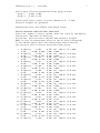
TROFSS program v. 2
10/12/2006
1
TROFSS User’s Guide
1. Description
TROFSS is a FORTRAN77 program that determines a point-wise approximation
to the PARETO SURFACE in SINGLE-STAGE PROBATIONARY or NON-PROBATIONARY selection decision when the applicant group is a MIXTURE OF MINORITY
AND MAJORITY APPLICANTS such that both the objectives of selection quality and
adverse impact are of importance. Selection quality can refer to either the predictor
composite validity, the globally standardized expected criterion performance or the utility
per selected applicant. The method of normal boundary intersection is used to determine
Pareto points that are evenly spread on the solution surface and for each point the
corresponding values of the selection rate (in case of a probationary selection decision),
the global criterion cutoff value and the predictor weights are computed.
At present, the program is limited to problems with no more than 10 selection predictors, a single majority and a single minority group and no more than 3 criterion behaviour
dimensions.
The effect sizes are defined with respect to the minority applicant group (i.e., the
first group) such that this group has all effect size values equal to zero. The computation
of the adverse impact ratio assumes that the last subgroup is the majority group.
The present program computes solutions over the entire set of feasible predictor
weights. Predictor weights are feasible if (a) at least one weight is positive and (b) all
weights are non-negative and at least equal to a given, non-negative value.
The FORTRAN77 program to implement the solution uses (a) routines from the
SLATEC FORTRAN77 library (Fong et al., 1993), (b) an extension of the algorithm
presented by Genz (2001) to compute multivariate probabilities, (c) the algorithm AS249
from the STATLIB software library and (d) bits of optimization code.
To implement the program, the user must specify a number of input parameter values.
These are detailed below. Among other things, the setting of the problem parameters
provides the opportunity to address probationary or non-probationary selections, to constrain the minimum and maximum hiring rate in the probationary period and to choose
between either the composite validity, the globally standardized expected criterion score
of the selected candidates or the selection utility as the selection quality criterion.
To derive the expected utility, the return of the corresponding random selection must
be computed first. This can be done using the program with certain specific values for
some of the input parameters (see below).
2. Assumptional Basis
The calculations are based on the assumption that the predictor and (eventually)
the criterion dimensions have a joint multivariate normal distribution with the same vari-
TROFSS program v. 2
10/12/2006
2
ance/covariance matrix but different mean vectors in the different applicant populations.
Given this assumption it is, without further restrictions, understood that the joint distribution of the predictors and the criterion dimensions is standard multivariate normal
in the reference applicant population (i.e., the minority applicant population).
3. Input
Observe that all input is in free format: Variables or vectores that have a
name commencing with the letters I, J, K, L, M, N get INTEGER values. All
other variables, vectors and matrices get FLOATING POINT values. See the
example input file.
• # 1: NC, IFIXCR, IFIB, IFIP, (VMAMI(I), I = 1, NGR)
– NC: number of criterion dimensions (NC ≤ 3)
– IFIXCR: The value of the composite criterion behaviour cutoff is estimated
(IFIXCR = 0) or given (IFIXCR = 1). For probationary selection set IFIXCR
= 0. For non-probationary selection, set IFIXCR = 1
– IFIB: Set IFIB = 0 in case of a non-probationary selection. Set IFIB = 1 in
case of a probationary selection for which the initial hiring rate is bounded
from below and above (see below)
– IFIP: Set IFIP = 0 in case of a non-probationary selection. Set IFIP = 1 in
case of a probationary selection for which the initial hiring rate is fixed at a
given value
– (VMAMI(I), I = 1, 2): VMAMI(I) indicates the proportion of the total
applicant group that comes from candidate population I Observe that
VMAMI(1) + VMAMI(2) must be equal to 1
• # 2: NPRED, IUTIL, IBN
– NPRED: the number of selection predictors. NPRED less or equal to 10.
– IUTIL: If IUTIL = 0, the globally standardized expected criterion score of the
selected applicants is used as the selection quality criterion. If IUTIL = 1,
selection quality corresponds to the selection utility per selected applicant.
To obtain the utility in monetary value, the utility must be multiplied by
the value of TFACC (see below). If IUTIL = -1, then the validity of the
composite predictor represents the selection quality objective.
– IBN: the number of points used to approximate the Pareto surface. Values
between 20 and 30 are usually adequate. The program always generated a
total of IBN + 1 points of the Pareto surface. If IBN = 1, only the two
TROFSS program v. 2
10/12/2006
3
extreme points of the Pareto surface are determined. IBN = 0 may only be
used in combination with IUTIL = 1.
• # 3: XSEL, VALLOW
– XSEL: Required proportion of successfully selected applicants
– VALLOW: Predictor weights must at least be equal to the value of VALLOW.
Normally, VALLOW = 0.
• # 4: OPTIONAL: only if IFIB is different from zero. The value of XOB. XOB
indicates the lower bound on the global selection ratio for probationary selections
• # 5: OPTIONAL: only if IFIB is different from zero. The value XUP. XUP
indicates the upper bound on the global selection ratio for probationary selections
• # 6 and following: OPTIONAL: only if IFIP is different from zero. The value
of XOB. XOB indicates the global selection ratio for probationary selections
• # 7 and following: For each applicant group K (with K = 1, 2), DIFC(K,I) (with
I = 1, NC), DIFP(K,I) (with I =1, NPRED).
The element DIFC(K,I) indicates the effect size value of criterion dimension I
for applicant group K, whereas DIFP(K,I) corresponds to the effect size value of
predictor I for the same candidate group. The elements of the first rows of DIFC
and DIFP are all zero because the first applicant group is the reference group. The
elements of the second row pertain to the majority applicant group that is used
to determine the adverse impact ratios.
• # 8: WC(I) (with I = 1, NC). Vector of length NC with the pre-assigned weights
of the criterion dimensions
• # 9 and following: CC(I,J) (with both I and J = 1, NC): NC × NC matrix of
criterion dimension intercorrelations. Only the strict upper triangle of the correlationmatrix! So, if NC = 1, then CC(1,1) must not be specified.
• # 10 and following: PC(I,J) (with both I and J = 1, NPRED). Matrix of predictor
correlations. Only the strict upper triangle of the correlationmatrix!
• # 11 and following: PV(I,J) (with I = 1, NC and J = 1, NPRED): matrix of
predictor validities. Thus PV(I,J) indicates the validity of predictor J with respect
to criterion dimension I.
• # 12: OPTIONAL: only if IUTIL = 1. The values of NAPPL, RETRAN,
SIY, XMUY, TFACC
TROFSS program v. 2
10/12/2006
4
– NAPPL: Total number of applicants
– RETRAN. RETRAN indicates the the payoff of the corresponding random
selection. To obtain the value of RETRAN, run the program with values of
1, 0 and 0. for IUTIL, IBN and RETRAN, respectively to compute the payoff
of a corresponding selection with a single, non-valid (i.e., predictor validity is
zero for all criteria) predictor with zero effect size.
– SIY: Money valued standard deviation of the criterion behaviour in the entire
applicant group for 1 time period
– XMUY: Money valued mean criterion behaviour in the entire applicant population for 1 time period
– TFACC: equate TFACC to XMUY
• # 13: OPTIONAL: only if IUTIL = 1. The values of RYR, TS
– RYR: Correlation between rated (aggregate or composite) criterion and money
valued criterion behaviour
– TS: Number of time periods that a successfully selected employee will remain
on the job.
• # 14: OPTIONAL: only if IUTIL = 1. The values of TRCO, SECO
– TRCO: Training costs per selected applicant
– SECO: Separation costs per unsuccessfully selected applicant
• # 15: OPTIONAL: only if IUTIL = 1. The values of TECO(I) (with I = 1,
NPRED): Vector of length NPRED with the predictor costs per applicant
4. Sample Input File
Important: in preparing the input file, use a simple text editor such as Notepad,
Wordpad or any other standard ASCII producing editor. DO NOT USE TEXT PROCESSING PROGRAMS SUCH AS MS-WORD or WORDPERFECT. Also, when saving
the input file in Notepad, use the option “All Files” in the “Save as type” box. When
saving in Wordpad, use the “Text Document-MS-DOS Format” option in the “Save as
type” box, and be aware that Wordpad has the nasty habit of adding the extension .txt to the file name that you specify. Thus, with Wordpad, if you specify the
name of the input file as “MINPUT”, the file will in fact be saved as “MINPUT.TXT”;
and this is the name that you have to use in the command to run the present programs.
Here is a sample input file, for the trofss program.
TROFSS program v. 2
2
1
0
0
4 0
20
0.15 0.
0.00
0.
0.210 0.130
3.000 1.000
0.170
0.240 0.000
0.120 0.160
0.510
0.300 0.300
0.160 0.260
5
10/12/2006
0.25
0.
1.000
0.75
0.
0.230
0.
0.090
0.
0.330
0.190
0.180
0.200
0.280
0.250
5. Running the Program
Suppose you copied the executable source of the program to the d:ssel directory
on your machine. In that case, the input file must also be saved in the d:ssel directory.
Next, to run the program, you have to open an MS-DOS Command window. The way
to do this varies from one operating system (i.e., Windows 95, 98, NT a.s.o.) to the
other, and you should use your local “HELP” button when in doubt about this feature.
In the MS-DOS Command window you type d:, followed by RETURN or ENTER,
and your computer will return the D:\> command prompt. Next, you type cd ssel after
the D:\> command prompt, again followed by RETURN or ENTER, and your computer
will respond with the D:\ssel> command prompt. Now, you can execute the program
by typing trofss < minput > moutput
where “minput” is the name of the input
file and “moutput” is the name of the output file. At the end of the execution, the PC
will return the command prompt D:\ssel>. You can then inspect the output by editing
the output file with either Notepad, Wordpad or any other simple editor program.
6. Sample Output
Program execution starts on
4/ 9/2006 at 16:59: 3
THE PRESENT CODE IS TO BE USED FOR RESEARCH PURPOSES ONLY
THE PROGRAM AUTOMATICALLY ABORTS AFTER SOME TIME AND
A NEW VERSION OF THE CODE MUST BE DOWNLOADED
++++++++++++
+ TROFSS +
+++++++++++++
Computation of the PARETO SURFACE in SINGLE-STAGE PROBATIONARY
or NON-PROBATIONARY selection decision when the applicant
group is a MIXTURE OF MINORITY AND MAJORITY APPLICANTS such
that both the objectives of selection quality and adverse
impact are of importance. Selection quality can refer to
TROFSS program v. 2
10/12/2006
6
either the globally standardized expected criterion
performance or the utility per selected applicant.
The method of normal boundary intersection is used to
determine Pareto points that are evenly spread on the
solution surface and for each point the corresponding
values of the selection rate (in case
of a probationary selection decision), the global
criterion cutoff value and the predictor weights are
computed.
Predictor weights obey a variance constraint.
At present, the program is limited to problems with no
more than 10 selection predictors, a single majority and
a single minority group and no more than 5 criterion
behaviour dimensions.
Program written by Wilfried De Corte, Ghent University,
Belgium
The program uses routines from the Slatec library (see
http://www.geocities.com/Athens/Olympus/5564), a couple
of algorithms from StatLib (see http://lib.stat.cmu.edu/apstat/),
and some (adapted) code from Genz to evaluate multivariate normal
probabilities (cf. http://www.math.wsu.edu/math/faculty/genz/homepage).
PROBLEM SPECIFICATION
Problem relates to a non-probationary selection
Quality Objective is Expected Criterion Score
Number of criterion dimensions: 2
Number of applicant groups: 2
Proportional representation applicant groups: 0.250 0.750
Overall proportion of (successful) selectees: 0.150
Number of available predictors: 4
Weights used to combine the individual criterion
dimensions to the composite criterion are:
3.000
1.000
Correlation matrix of the criterion dimensions:
Criterion 1
1.000 0.170
Criterion 2
0.170 1.000
Correlation matrix of the predictors:
Predictor 1
1.000 0.240 0.000 0.190
Predictor 2
0.240 1.000 0.120 0.160
Predictor 3
0.000 0.120 1.000 0.510
Predictor 4
0.190 0.160 0.510 1.000
Validities of the predictors (columns) with respect
to the criterion dimensions (rows):
Criterion 1
0.300 0.300 0.180 0.280
Criterion 2
0.160 0.260 0.200 0.250
Effect sizes selection predictors (First group is base)
Group 1:
0.000 0.000 0.000 0.000
Group 2:
1.000 0.230 0.090 0.330
TROFSS program v. 2
7
10/12/2006
Effect sizes criterion dimensions (First group is base)
Group 1:
0.000 0.000
Group 2:
0.210 0.130
Fixed cutoff value overall criterion dimension is
Predictor weights are optimized
-7.500
Computations start from random initialized values
DETAILS SELECTED PARETO-OPTIMAL TRADE-OFFS
First line: number of Pareto-optimal trade-off, Value AI and Quality,
and Relative Importance AI Objective
Second line: Selection ratio and Unit Sum Predictor Weights
NOTE: In case of probationary selection the AI value corresponds
to the adverse impact after the probationary period, whereas
the selection ratio is before the probationary period.
1
2
3
4
5
6
7
8
9
10
11
12
13
14
15
16
17
AI Quality
0.150
AI Quality
0.150
AI Quality
0.150
AI Quality
0.150
AI Quality
0.150
AI Quality
0.150
AI Quality
0.150
AI Quality
0.150
AI Quality
0.150
AI Quality
0.150
AI Quality
0.150
AI Quality
0.150
AI Quality
0.150
AI Quality
0.150
AI Quality
0.150
AI Quality
0.150
AI Quality
0.868
0.000 0.000
0.850
0.000 0.056
0.833
0.000 0.110
0.815
0.000 0.162
0.798
0.000 0.213
0.780
0.000 0.264
0.762
0.000 0.318
0.743
0.000 0.375
0.724
0.000 0.442
0.703
0.000 0.536
0.678
0.000 0.546
0.651
0.000 0.536
0.623
0.000 0.526
0.592
0.000 0.512
0.554
0.021 0.493
0.515
0.053 0.474
0.476
0.350
1.000
0.380
0.944
0.410
0.890
0.439
0.838
0.468
0.787
0.498
0.736
0.527
0.682
0.556
0.625
0.584
0.558
0.611
0.464
0.635
0.403
0.658
0.347
0.680
0.283
0.699
0.199
0.713
0.162
0.727
0.157
0.740
Rel. Import.
0.000
Rel. Import.
0.000
Rel. Import.
0.000
Rel. Import.
0.000
Rel. Import.
0.000
Rel. Import.
0.000
Rel. Import.
0.000
Rel. Import.
0.000
Rel. Import.
0.000
Rel. Import.
0.000
Rel. Import.
0.052
Rel. Import.
0.116
Rel. Import.
0.191
Rel. Import.
0.289
Rel. Import.
0.323
Rel. Import.
0.316
Rel. Import.
AI 1.000
AI 0.628
AI 0.627
AI 0.626
AI 0.624
AI 0.620
AI 0.614
AI 0.604
AI 0.583
AI 0.513
AI 0.477
AI 0.456
AI 0.419
AI 0.329
AI 0.262
AI 0.253
AI 0.241
TROFSS program v. 2
18
19
20
21
0.150
AI Quality
0.150
AI Quality
0.150
AI Quality
0.150
AI Quality
0.150
8
10/12/2006
0.087 0.454
0.435
0.123 0.432
0.393
0.164 0.407
0.348
0.213 0.378
0.296
0.277 0.339
CPU TIME IN SECONDS
0.151
0.752
0.146
0.763
0.139
0.772
0.131
0.777
0.120
0.308
Rel. Import.
0.300
Rel. Import.
0.290
Rel. Import.
0.279
Rel. Import.
0.264
AI 0.222
AI 0.192
AI 0.136
AI 0.000
2.88
7. Description of Output
At present, the output provides input for plots of the solution using the R package.
8. Acknowledgement
When the user reports results obtained by the present program, due reference should be made to De Corte (2006) and De Corte, Lievens & Sackett
(2007).
11. References
De Corte, W. (2006). TROFSS User’s Guide.
De Corte, W., Lievens, F. & Sackett, P. (2007). Combining predictors to achieve
optimal trade-offs between selection quality and adverse impact. Journal of Applied
Psychology (accepted)
Fong, K. W., Jefferson, T. H., Suyehiro, & Walton, L. (1993). Guide to the SLATEC
common mathematical library (http://www.netlib.org/slatec/).