Download A user guide for the ACCESS land surface model Community

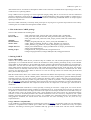
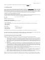
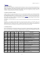
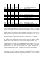
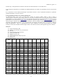
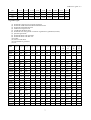
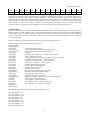
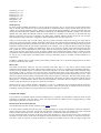
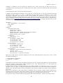
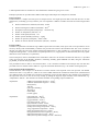
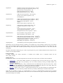
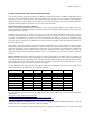
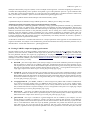
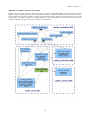
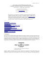
CABLE user guide v1.3
A user guide for the ACCESS land surface model
Community Atmosphere Biosphere Land Exchange (CABLE)
Gab Abramowitz1,2, Yingping Wang2 and Bernard Pak2
2
1
University of New South Wales
CSIRO Marine and Atmospheric Research
[email protected]
For CABLE version 1.3 – October 2007
This document is a user guide for the Community Atmosphere Biosphere Land Exchange
(CABLE) land surface model. It is likely to be changing regularly as CABLE itself is
updated – please check the ACCESS website to make sure you have the latest version. It
compliments CSIRO Marine and Atmospheric Research paper 013 (Kowalczyk et al, 2006)
which provides a full technical description of CABLE as well as its development history. It
is intended to help users understand the workings of CABLE and speed its implementation.
The authors, however, assume no responsibility for results which arise from its use.
0. Introduction
1. Files in the basic CABLE package
2. Driving CABLE
3. Compiling CABLE
4. General considerations when running CABLE
5. Temporal and spatial variables
6. CABLE parameters
7. Initialisation, spin-up and restart files
8. Input and output
9. Addressing parameter uncertainty/calibrating CABLE
10. Viewing CABLE's output and judging performance
References
A1. CABLE's structure and coding
0. Introduction
Like most land surface models (LSMs), CABLE simulates the exchanges of radiation, moisture, heat and carbon at the
land surface. It is provided with meteorological conditions (its inputs) and, based on these, predicts fluxes (its outputs,
e.g. latent heat flux, upward long-wave radiation, net ecosystem exchange of CO2 or drainage through deep soil). The
characteristics of the soil and vegetation in the regions it simulates are for the most part constant throughout the
simulation, and described by CABLE's parameters. Variables which CABLE stores in memory from one time step to the
next, known as model states, include soil moisture content, soil and vegetation temperatures, and carbon stored in the
vegetation and soil. An abstract schematic representation of these model components is shown in Figure 1.
Figure 1: A schematic representation of a model,
with real number inputs, outputs, states and timeindependent parameters.
Ultimately, CABLE is designed to work as a single component of a larger global climate model (GCM). In this
situation, CABLE receives meteorological data from, and passes flux information to, a boundary layer atmospheric
model. When coupled to such a model, CABLE is said to be running 'online'. Alternatively, meteorological data from
1
CABLE user guide v1.3
observational sites or saved from an atmospheric model can be used to force CABLE and its output simply saved to file,
in which case it is operating 'offline'.
Using CABLE involves agreeing to a license agreement (largely stating that its use will not be used for commercial
purposes); obtaining a password to the cable user site and downloading the code; getting CABLE to compile using a
Fortran 90 compiler and netcdf distribution on your own machine; and running with default datasets to compare against
operating benchmark runs.
Since the CABLE community is relatively small, please pass on any bug fixes or genuine improvements to the code by
contacting the core CABLE team through the CABLE website.
1. Files in the basic CABLE package
The set of files should look something like:
Core code:
Drivers and i/o:
Makefile:
Documentation:
Surface data:
Sample data sets:
Plotting scripts:
cable_carbon.f90; cable_soilsnow.f90; cable_cbm.f90; cable_variables.f90;
cable_driver.f90; cable_drivertxt.f90; cable_parameters.f90; cable_input.f90;
cable_output.f90; cable_checks.f90; cable_output_text.f90; cable.nml; cabletxt.nml;
Makefile;
CABLE_userguide.pdf; End_user_licence_terms.pdf; READMEv1.3;
surface_data/LAI_Monthly_Global.nc; surface_data/def_soil_params.txt;
surface_data/def_veg_params.txt; surface_data/VegSoil_Type_Global.txt;
sample_met/Tumbarumba.nc; sample_met/Bondville.nc; sample_met/Tharandt.nc;
sample_met/Tumbarumba.txt;
testing/diurnal.R; testing/seasonal.R; testing/timeseries.R
testing/averagingwindow.R; testing/CABLEplots.R; testing/generalTest.R
2. Driving CABLE
Using CABLE offline
There are two example offline drivers provided to help run CABLE; one with netcdf input/output and one with text
input/output. It is recommend that users choose the netcdf driver where possible, particularly if they are not familiar
with CABLE. In the netcdf driver, all input data and running variables (spatial and temporal details) are retrieved from a
netcdf file/s - the user does not then need to compile the code more than once. It also produces netcdf output with a
choice which output variables are to be written, with variable units included in the file. In the text driver, the running
variables must be set manually inside the driver code, with meteorological data read from a formatted text file. These
processes are described in more detail in Sections 4-8. The two driving routines are named cable_driver.f90 and
cable_drivertxt.f90 respectively.
Both the netcdf and text driver use a namelist file (cable.nml and cabletxt.nml respectively) to read in some operating
variables. Also, both may call the “default_params” subroutine (in cable_variables.f90) to generate default parameter
and initial values for a run if no other source is found (see Sections 6 and 7). These values may not be appropriate for
your application. Both will also produce a log file (named “log_cable.txt” by default – can be changed in the namelist
file – see Section 4) which lists the parameter values read for each grid cell in the simulation, as well as the initial states.
By default, the included Makefile will compile the netcdf version. To compile one or the other, type "make netcdf" or
"make text".
It is recommended that netcdf driver is used, especially if running at more than a single point, for several reasons.
Firstly, all spatial and temporal timing variables are guaranteed to be set, as the netcdf version will not run if they are
not present or consistent. Next, the ranges and units of all input met and output variables will be checked as they are
read and written. Lastly, the netcdf version prints a more detailed log file which reports any discrepancies during
execution, as well as all model parameters and variable initialisations. The text version, by comparison, uses a quick
and dirty (and much simpler) driver and i/o routine - for confident users. Somewhere between a one-gridpoint and a
many-gridpoint simulation, the netcdf routine will become the less time consuming of the two, even for very
experienced users.
Using CABLE in a coupled model
To use CABLE as a coupled model keep in mind the five points in Section 4. In particular, make sure your atmospheric
variables are compatible with CABLE's grid. CABLE uses a land-only grid and its variables have only one spatial
dimension. Translating a land-sea grid to CABLE's land-only grid can be made easier with the Fortran commands
2
CABLE user guide v1.3
“PACK” and “UNPACK”. Spatial and temporal variables are discussed in Section 5 below.
3. Compiling CABLE
Notes on using netcdf - To use the netcdf driver for CABLE you must have a netcdf installation available. The netcdf
package must be compiled with access to the same Fortran 90 compiler you are using to compile CABLE. The netcdfbased CABLE driver (using "make" or "make netcdf") uses the netcdf Fortran 90 interface. There must be a symbolic
link to "netcdf.mod" (part of the netcdf installation) in the directory in which you want to compile CABLE. In addition,
you will need to change the netcdf path in the Makefile to reflect the location of your netcdf installation.
Compiling with the supplied Makefile (linux/unix)
To use the Makefile, all that should be required is to modify the Makefile to reflect the command line Fortran compiler
you wish to use, and, if you are using netcdf, the path of the netcdf installation. For example:
FC = g95
FFLAGS =
NCDIR = /usr/local/netcdf-3.6.1/
# e.g. 'g95' or 'ifort' or 'lf95' etc.
Compiling without the Makefile
The order of file compilation for CABLE is as follows:
1. cable_variables.f90
2. cable_soilsnow.f90, cable_carbon.f90, cable_parameters.f90 (each of these depend only on cable_variables)
3. cable_cbm.f90
4. cable_checks.f90
For netcdf i/o:
5. cable_input.f90
6. cable_output.f90
7. cable_driver.f90
For text i/o:
5. cable_output_text.f90
6. cable_drivertxt.f90
This information can be inferred from the supplied Makefile or the CABLE structure diagram in Appendix 1.
The code has been tested to compile and run on Windows (Compaq, g95, Intel & Lahey/Fujitsu compilers), Mac OSX
(g95, ifort), linux/unix (Intel[ifort], SUNws[f95], Lahey/Fujitsu[lf95], g95), and NEC SX6.
4. General considerations when running CABLE
Whether you intend to run CABLE offline or online, there are five broad areas where problems may arise:
a) Model parameters – CABLE has a lengthy list of parameters which describe the soil and vegetation
characteristics of the region(s) it simulates. These parameters should be set to best represent the conditions of
your simulation. A full list of these, including their definitions and variable names within CABLE's code, is
given in Section 6 below. A subroutine is provided to read default values of CABLE's parameters from a coarse
global grid based on latitude and longitude (more detail in Section 6). These are NOT appropriate for all
applications.
b) Initialisation – a collection of model states (e.g. soil moisture and soil temperature) need to be given initial
values. A full list of these and a discussion of the provided default initialisation routine is given in Section 7. It
is recommended that in addition to prescribing initial values for model states, users spin-up the model states
(using at least one year of input data) until they reach equilibrium. The netcdf driver has a facility for setting
spin-up sensitivity and the use of restart file. More detail is given in Section 7.
c) Meteorological input – CABLE's input is a collection of meteorological variables. These need to be read in to
CABLE's 'met' arrays with the correct units. Details are given in Section 8.
d) Temporal and spatial variables – ensure that CABLE's time step size, run length, number of gridpoints and
gridpoint details are compatible with your simulation. Instructions for changing these are given in Section 5.
e) Output – CABLE's output obviously needs to be of a nature and in a format that you can process and is useful
for your application, including variable units. Options for output are discussed in Section 10.
Making sure that these areas are appropriately configured for your application is your responsibility. Plotting CABLE's
output in a variety of measures to make sure it is behaving properly is essential. Example plotting scripts are described
3
CABLE user guide v1.3
in Section 10.
Log file and diagnostics:
There are two levels of diagnostics. Permissible runtime comments are written to the log file (name determined in the
namelist file cable.nml), whilst serious and/or fatal errors are printed to screen. The log file contains details of timing,
locations, initialisations and parameters used during simulation. If using the netcdf driver with many sites being
simulated, writing of each site's initialisations and parameter values can be suppressed by setting “verbose” to
“.FALSE.” in cable.nml namelist file to avoid a very large log file.
5. Temporal and spatial variables
CABLE's variables use a single spatial dimension. That is, for regional/global simulations, the two dimensional latitude
and longitude based grid needs to be mapped to a single 'line' of sites. The provided netcdf driver automatically maps
from latitude/longitude references in the netcdf input file to a single dimension. It can do so either with the use of a
'mask' variable or through an ALMA-style compressed land grid (see Section 8). Fortran 'pack' and 'unpack' functions
may be useful when doing this manually for coupled runs. The single dimension allows CABLE to run for the entire
region/globe in a single subroutine call.
Netcdf driver - The netcdf offline driver will set all temporal and spatial variables from data in the meteorological data
input file.
Text driver – In the supplied text-based offline driver, temporal and spatial variables are set manually, either in the
namelist file cabletxt.nml which the driver reads, or in the fortran code itself. The user must set: ‘mp’ – the number of
land grid points; ‘dels’ – time step size; ‘kend’ – the number of time steps in the run; 'latitude' and 'longitude' for each
grid cell/site simulated as well making sure all grids map consistently between input and output.
6. CABLE parameters
Each one of the parameters in the table below needs to be set to represent the site(s)/region(s) being simulated. CABLE
has “mp” land points and “ms” soil layers. Note that the ranges here are “physically possible” ranges for the entire
globe – they are not likely to be appropriate for automated parameter estimation in most circumstances. Ensuring the
appropriate parameters are used for an individual application is the user's responsibility.
name
type
dimension
units
ranges
albsoil
real
(mp)
-
0.1 – 0.4
bch
real
(mp)
-
4 - 15
parameter b in Campbell equation
clay
real
(mp)
-
0-1
fraction of soil which is clay
css
real
(mp)
kJ/kg/K
800 - 2500
-6
description
-3
snow free shortwave soil reflectance (fraction)
soil specific heat capacity
hyds
real
(mp)
m/s
10 - 10
isoilm
int
(mp)
-
1-9
ratecs
real
(mp,2)
1/year
0.001 – 5.0
soil carbon pool rate constant
rhosoil
real
(mp)
kg/m3
500 - 2500
soil bulk density
rs20
real
(mp)
-
0.01-10
sand
real
(mp)
sfc
real
(mp)
silt
real
(mp)
3
m /m
0-1
3
3
ssat
real
(mp)
m /m
sucs
real
(mp)
m
3
swilt
real
(mp)
m /m
zse
real
(mp,ms)
m
0.1 – 0.5
0-1
3
3
0.1 - 0.6
hydraulic conductivity @ saturation
Soil type
NOT CURRENTLY USED [soil respiration scaler]
fraction of soil which is sand
vol H2O @ field capacity
fraction of soil which is silt
vol H2O @ saturation
-0.7 - -0.1
suction at saturation
0.05 - 0.4
vol H2O @ wilting
currently fixed thickness of each soil layer
4
CABLE user guide v1.3
canst1
real
(mp)
mm/LAI
0.08 - 0.12
max intercepted water by canopy
dleaf
real
(mp)
m
0.005 - 0.2
characteristic length of leaf
max pot. electron transport rate top leaf
2
ejmax
real
(mp)
mol/m /s
1e-5 - 3e-4
frac4
real
(mp)
-
0-1
fraction of c4 plants
froot
real
(mp,ms)
-
0-1
fraction of root in each soil layer
hc
real
(mp)
m
0 - 100
height of canopy
iveg
int
(mp)
-
1- 13
Vegetation type
meth
int
(mp)
-
ratecp
real
(mp,3)
1/year
0.02 – 2.0
rp20
real
(mp)
-
0.01-10
plant respiration scaler
rpcoef
real
(mp)
1/C
0.03-0.2
NOT CURRENTLY USED [temperature coef for
non-leaf plant respiration]
shelrb
real
(mp)
-
0.5 – 2.0
sheltering factor
tminvj
real
(mp)
C
-5 – 10
min temperature of the start of photosynthesis
tmaxvj
real
(mp)
C
15 - 40
max temperature of the start of photosynthesis
vbeta
real
(mp)
-
1- 20
vcmax
real
(mp)
mol/m2/s
5e-6 - 1.5e-4
xfang
real
(mp)
-
-1.0 - 1.0
za
real
(mp)
m
1-100
currently fixed method for calculation of canopy fluxes and temp
plant carbon pool rate constant
stomatal sensitivity to soil water
maximum RuBP carboxylation rate top leaf
leaf angle parameter
reference height/lowest level of atmospheric model
CABLE's parameters can be loaded from one of three sources: the meteorological forcing file; a restart file (see
'Initialisation' section), or; using values extracted from a coarse global grid, based on soil and vegetation types
(provided). It is recommended that users at least specify correct soil and vegetation types for their site(s) of simulation
(ideally derive their own parameter sets for all of the above variables), for all but global simulations.
Ideally, one would have enough information about the sites/region being simulated to provide reasonable values for the
parameters listed above. This is often not the case, however. In deciding the parameter values for any given grid cell, in
the first instance we suggest using the appropriate soil and vegetation type (shown below) for that grid cell. Then, adjust
those parameters for which site-specific information is available. Care needs to be taken to avoid inconsistencies (e.g. in
the relationship between wilting point, field capacity and soil saturation values or soil, silt and sand fractions). Also note
that the reference height “za” is not prescribed by either vegetation or soil types, and must be set appropriately. Once
this “best guess” parameter set is defined, we suggest adding it to the meteorological data file, as described below.
Prescribing CABLE's parameters
To prescribe CABLE's parameters, they need to be added/present in the meteorological forcing file or the restart file
(see 'Initialisation' section). As the restart file may be overwritten, we suggest the best method is to include the
parameters in the met file. Any restart file generated using this met file will then inherit these parameter values.
When the netcdf driver loads parameters it gives first preference to any values found in the met file, then values the
restart file, and lastly to the default values described below (if no restart file is present). Any restart file must have a
complete set of parameters (as restart files written by the netcdf driver do), whereas the met file may have only a subset
of CABLE's parameters. When prescribing only a subset of the parameters in the met file, take care to avoid parameter
inconsistencies, such as those described above. If no restart file is found, for example, the remaining subset of
unprescribed parameter values will be loaded from the default grid (described below), which may give inappropriate
vegetation and soil types for your site. A specification of 'isoil' and/or 'iveg' (soil and vegetation type) in the met file
will load all parameters associated with that type – any additional parameter specifications will overwrite these.
Both the meteorological forcing file and the restart file for the netcdf driver are netcdf. The variable names for each of
the parameters are as listed in the table above, all lower case. They of course (being parameters) have no time
dimension. Spatial representation in the met file is dependent on whether an x-y grid with land/sea mask or a land-only
vector (essentially as shown in the table above, with dimension 'mp') is used. Please see the “Input and output” section
below for the distinctions between these two spatial representations. Spatial representation in the restart file will always
5
CABLE user guide v1.3
be land-only, so that parameters stored there will have the same dimensions as in the table above.
In the sample text-based driver for CABLE, non-default parameters will need to be specified by the user in the Fortran
code.
For a discussion on more advanced techniques of parameter selection, such as automated calibration or parameter
perturbed ensembles, see section 9 below.
Using the default parameter sets from the default grid
As mentioned above, each of the provided driver routines for running CABLE offline is able to utilise a
“default_params” subroutine which collects values for each of the parameters above, point by point, based on latitude
and longitude. For a given simulation grid point, this subroutine first locates the closest grid point in a coarse (2º by 2º)
global map of nine soil (based on Zobler (1998)) and thirteen vegetation types (based on Potter et al (1993)) and then
uses these types to infer the above parameters. Note that these values are unlikely to appropriate in most circumstances,
particularly using different grid sizes. Care should be taken, for example, using these coarse grid parameter values for
single site applications – there is no guarantee that the correct vegetation or soil type will be chosen, for example.
Currently, all sites have a default reference height of 40m. The values for each soil and vegetation type are as follows:
Soil types:
(1)
(2)
(3)
(4)
(5)
(6)
(7)
(8)
(9)
Coarse sand/Loamy sand
Medium clay loam/silty clay loam/silt loam
Fine clay
Coarse-medium sandy loam/loam
Coarse-fine sandy clay
Medium-fine silty clay
Coarse-medium-fine sandy clay loam
Organic peat
Permanent ice
SOIL
Type 1
Type 2
Type 3
Type 4
Type 5
Type 6
Type 7
Type 8
Type 9
albsoil
0.1
0.1
0.1
0.1
0.1
0.1
0.1
0.1
0.1
bch
4.2
7.1
11.4
5.15
10.4
10.4
7.12
5.83
7.1
clay
0.09
0.30
0.67
0.20
0.42
0.48
0.27
0.17
0.30
css
850
850
850
850
850
850
850
1920
2100
166.0
4.0
1.0
21.0
2.0
1.0
6.0
800.0
1.0
hyds * 10-6
isoilm
1
2
3
4
5
6
7
8
9
ratecs1
2.0
2.0
2.0
2.0
2.0
2.0
2.0
2.0
2.0
ratecs2
0.5
0.5
0.5
0.5
0.5
0.5
0.5
0.5
0.5
ratecs3
0.004
0.004
0.004
0.004
0.004
0.004
0.004
0.004
0.004
rhosoil
1600
1600
1600
1600
1600
1600
1600
1300
910
rs20
1.0
1.0
1.0
1.0
1.0
1.0
1.0
1.0
1.0
sand
0.83
0.37
0.16
0.60
0.52
0.27
0.58
0.13
0.37
sfc
0.143
0.301
0.367
0.218
0.31
0.37
0.255
0.45
0.301
silt
0.08
0.33
0.17
0.20
0.06
0.25
0.15
0.70
0.33
ssat
0.398
0.479
0.482
0.443
0.426
0.482
0.420
0.451
0.479
sucs
-0.106
-0.591
-0.405
-0.348
-0.153
-0.49
-0.299
-0.356
-0.153
swilt
0.072
0.216
0.286
0.135
0.219
0.283
0.175
0.395
0.216
zse 1
0.022
0.022
0.022
0.022
0.022
0.022
0.022
0.022
0.022
zse 2
0.058
0.058
0.058
0.058
0.058
0.058
0.058
0.058
0.058
6
CABLE user guide v1.3
zse 3
0.154
0.154
0.154
0.154
0.154
0.154
0.154
0.154
0.154
zse 4
0.409
0.409
0.409
0.409
0.409
0.409
0.409
0.409
0.409
zse 5
1.085
1.085
1.085
1.085
1.085
1.085
1.085
1.085
1.085
zse 6
2.872
2.872
2.872
2.872
2.872
2.872
2.872
2.872
2.872
Vegetation types:
(1) broad-leaf evergreen trees (tropical rainforest)
(2) broad-leaf needle-leaf and broad-leaf deciduous trees
(3) broad-leaf and needle-leaf trees
(4) needle-leaf evergreen trees
(5) needle-leaf deciduous trees
(6) broad-leaf trees with ground cover/short-vegetation/C4 grassland (savanna)
(7) perennial grasslands
(8) broad-leaf shrubs with grassland
(9) broad-leaf shrubs with bare soil
(10) tundra
(11) bare soil and desert
(12) agricultural/c3 grassland
(13) ice
VEG
Type 1 Type 2 Type 3 Type 4 Type 5 Type 6 Type 7 Type 8 Type 9 Type
10
canst1
0.1
0.1
0.1
0.1
0.1
0.1
0.1
0.1
0.1
0.1
0.1
0.1
0.1
dleaf
0.075
0.12
0.07
0.028
0.02
0.16
0.16
0.155
.0165
0.155
0.005
0.155
0.005
170.0
160.0
130.4
140.0
20.2
18.0
70.106
78.0
76.106 34.04
240.0
2.0
ejmax * 170.0
10-6
Type
11
Type
12
Type
13
frac4
0.0
0.0
0.0
0.0
0.0
1.0
1.0
0.0
0.0
0.0
0.0
0.0
0.0
hc
35.0
20.0
20.0
17.0
17.0
1.0
0.5
0.6
0.5
4.0
0.05
1.0
0.01
iveg
1
2
3
4
5
6
7
8
9
10
11
12
13
meth
0
0
0
0
0
0
0
0
0
0
0
0
0
ratecp1 1.0
1.0
1.0
1.0
1.0
1.0
1.0
1.0
1.0
1.0
1.0
1.0
1.0
ratecp2 0.03
0.03
0.03
0.03
0.03
0.03
0.03
0.03
0.03
0.03
0.03
0.03
0.03
ratecp3 0.14
0.14
0.14
0.14
0.14
0.14
0.14
0.14
0.14
0.14
0.14
0.14
0.14
rp20
1.1342 1.4733
2.3704
3.3039
3.2879 1.0538
0.8037
12.032
1.2994
7.4175 2.8879
3.0
0.10
rpcoef
0.0832 0.0832
0.0832
0.0832
0.0832 0.0832
0.0832
0.0832
0.0832
0.0832 0.0832
0.0832
0.0832
shelrb
2.0
2.0
2.0
2.0
2.0
2.0
2.0
2.0
2.0
2.0
2.0
2.0
2.0
tminvj
5.0
5.0
5.0
2.0
5.0
10.0
10.0
0.0
5.0
-5.0
5.0
10.0
-5.0
tmaxvj
15.0
15.0
10.0
5.0
10.0
15.0
15.0
5.0
10.0
0.0
10.0
15.0
0.0
vbeta
1.0
1.0
1.0
1.0
1.0
4.0
4.0
4.0
4.0
1.0
4.0
4.0
1.0
vcmax
* 10-6
85.0
85.0
80.0
65.2
70.0
10.1
9.0
35.053
39.0
38.053 17.02
120.0
1.0
xfang
0.1
0.25
0.125
0.01
0.01
-0.3
-0.3
0.2
0.01
0.2
0.01
-0.3
0.01
froot 1
0.02
0.04
0.04
0.04
0.04
0.05
0.05
0.05
0.05
0.05
0.05
0.05
0.05
froot 2
0.06
0.11
0.11
0.11
0.11
0.15
0.15
0.10
0.10
0.10
0.10
0.15
0.15
froot 3
0.14
0.20
0.20
0.20
0.20
0.35
0.35
0.35
0.35
0.35
0.35
0.34
0.35
froot 4
0.28
0.26
0.26
0.26
0.26
0.39
0.39
0.35
0.35
0.35
0.35
0.38
0.40
7
CABLE user guide v1.3
froot 5
0.35
0.24
0.24
0.24
0.24
0.05
0.05
0.10
0.10
0.10
0.10
0.06
0.04
froot 6
0.15
0.15
0.15
0.15
0.15
0.01
0.01
0.05
0.05
0.05
0.05
0.02
0.01
Note that the parameter values associated with a particular vegetation and/or soil type will be used if that type is
specified in the met forcing file (while using the netcdf driver). Any additional parameter specifications in the met file
will overwrite these values. For example, if 'isoil' is present in the met file and set to be '2' (Medium clay loam/silty clay
loam/silt loam), all those parameter values associated with soil type 2 will be set (e.g. bch=7.1). If 'bch' is also present
in the met file, say set as bch=6.5, then 6.5 will be used. Note the danger this poses in terms of possible inconsistent
parameter values (e.g. setting clay=0.4 in addition to isoil=2 will result in clay+silt+sand not equal to 1).
7. Initialisation
Below is a complete list of variables that need to be initialised. Both of the provided drivers utilise the subroutine
'default_params' (in cable_parameters.f90), which will initialise these variables using values from a global simulation
using CABLE coupled to CCAM. They help CABLE avoid instability/oscillations during the first few time steps, but
are very crude and of course not accurate initial states for any point in time; making sure CABLE is properly initialised
is your responsibility.
The list of variables to be intialised (all of dimension 'mp', unless stated otherwise) is:
canopy%cansto canopy water storage (mm or kg/m2)
canopy%sghflux
canopy%ghflux
ssoil%ssdnn
overall snow density (kg/m3)
ssoil%snowd
snow liquid water equivalent depth (mm or kg/m2)
ssoil%osnowd
snowd from previous timestep (mm or kg/m2)
ssoil%snage
snow age
ssoil%isflag
snow layer scheme flag (0 = no or little snow, 1=snow)
ssoil%wbice
soil ice - dimension (mp,6)
ssoil%tggsn
snow temperature per layer (K) – dimension (mp,3); 3 soil layers
ssoil%ssdn
snow density per layer (kg/m3) – dimension (mp,3)
ssoil%smass
snow mass per layer (kg/m2) – dimension (mp,3)
ssoil%runoff
runoff total = subsurface + surface runoff
ssoil%rnof1
surface runoff (mm/timestepsize)
ssoil%rnof2
deep drainage (mm/timestepsize)
ssoil%rtsoil
turbulent resistance for soil
canopy%ga
ground heat flux (W/m2)
canopy%dgdtg
derivative of ground heat flux wrt soil temp
canopy%fev
latent heat flux from vegetation (W/m2)
canopy%fes
latent heat flux from soil (W/m2)
canopy%fhs
sensible heat flux from soil (W/m2)
ssoil%albsoilsn
albedo of soil+snow – dimension (mp,3); 3 radiation bands
ssoil%wb
soil moisture – dimension (mp,6)
ssoil%tgg
soil temperature – dimension (mp,6)
bgc%cplant
plant carbon (g C/m2) – dimension (mp,ncp)
bgc%csoil
soil carbon (g C/m2) – dimension (mp,ncs)
bal%wbtot0
bal%osnowd0
and the following cumulative variables need to be initialised at 0.0:
sum_flux%sumpn = 0.0
sum_flux%sumrp = 0.0
sum_flux%sumrpw = 0.0
sum_flux%sumrpr = 0.0
sum_flux%sumrs = 0.0
sum_flux%sumrd = 0.0
sum_flux%dsumpn = 0.0
sum_flux%dsumrp = 0.0
sum_flux%dsumrd = 0.0
8
CABLE user guide v1.3
bal%precip_tot = 0.0
bal%rnoff_tot = 0.0
bal%evap_tot = 0.0
bal%wbal_tot = 0.0
bal%ebal_tot = 0.0
bal%drybal = 0.0
bal%wetbal = 0.0
Model spin-up
For most purposes CABLE should have a 'spin-up' period, forced with a year (or several years) of meteorological data
until its internal states stabilise. To this end, the netcdf driver namelist file has a logical variable which may be set to
'.TRUE.' for a (limited) automatic spin-up. The driver will then run the specified 'filename_met' file repeatedly until soil
moisture and soil temperature stabilise. Stabilisation is defined by the 'delsoilM' and 'delsoilT' variables, set in the same
namelist file. They define the allowed variation in each of these two variables in any soil layer in the final time step
between consecutive spin-up runs of filename_met. When these variables stabilise, the data set will be run one more
time and output written. Note that in a regional or global simulation this may take some time!
There are several reasons why a model spin-up may not produce reasonable initial states. Firstly, the input data set
period may not be representative. Ideally, the model would spin-up using observed meteorological forcing data from the
period preceding the simulation period that the states be as realistic as possible. Using the same data set for spin-up and
simulation could mean that the soil moisture initialisation, for example, is too dry when the data set represents drought
years. To try to avoid this problem, the netcdf driver looks for an 'avPrecip' variable in the meteorological input file.
This variable has no time dependence (it has a single value for each grid cell) and represents the average precipitation
value for the particular grid cell/site, in mm. If 'spinup=.TRUE' in the namelist file and the 'avPrecip' variable is found,
precipitation values read from the meteorological data input file will be rescaled to match this value, for the duration of
the spin-up only. If information of rainfall patterns in the pre-simulation period is available, avPrecip should be set
appropriately.
In addition, CABLE, like any other natural system model, produces biases in its input-state mapping and so the states
are likely to 'drift' from true values.
Restart files
The offline netcdf driver allows for the use of (netcdf) restart files. That is, a file may be read in before model
simulation which contains initial state values for the variables above, as well as a complete set of CABLE's parameters.
The driver will by default look for a restart file whose name and path is set in the cable namelist file (cable.nml) using
the 'filename_restart_in' variable. If no such file exists, the default (and rather crude) initial values read in through
cable_parameters.f90 will be used. To create a restart file, simply set the logical variable 'output%restart' to true – then
when a run finishes, the final states and parameters used will be written to a restart file. The name of the output restart
file is set by the 'filename_restart_out' variable in the namelist file. This facility is useful in conjunction with the spin-up
facility above – if output%restart=.TRUE. for the spin-up simulation, when states have converged, a restart file will be
written saving the need to spin-up again if a repeat run is required.
Restart files also store CABLE parameter information, so that if a combination of prescribed and default parameters
was used in the initial run (see section on parameters, above), when the restart file is loaded for the new run, the
availability of these parameters may negate the need to load the default grid, saving time.
8. Input and output
If you intend to use CABLE with the text-based offline driver or coupled to an atmospheric model, the mode of input
and output is essentially your own choice. Since the safest execution of CABLE involves using/producing a netcdf
meteorological data file, we discuss this first:
Details about the netcdf met data file
The netcdf format used here broadly conforms to the ALMA standard.
1. It must contain a double precision real "time" variable, dependent on a single time dimension (name not important),
which is the time value, in seconds, of each time step since the starting time value. The starting time value is obtained
from the "units" field for the "time" variable, and is of the form: "seconds since 2001-02-22 00:01:00".
It is not essential that this "start time" be the start time of the simulation, e.g. the first value of the "time" variable may
be 86400, in which case the actual start time might be 2001-02-22 00:01:00 + 86400 seconds; i.e. 2001-02-23 00:01:00.
The "time" value for regional or global simulations is assumed to be GMT, while the value for single site/grid cell
9
CABLE user guide v1.3
simulations is assumed to be local. Single site simulation "time" values will be read as GMT if and only if a
"coordinate" field is present for the "time" variable and set to be "GMT". This time coordinate system will be reported
in the log file.
2. The met data file name is set in the cable.nml namelist file.
3. Multiple site/regional/global simulations can use either an x-y grid input file or a land only compressed grid-type
input file. For the x-y grid, an "x" and a "y" dimension must be present, even if the simulation is only a single
site/gridpoint. Additionally, single precision variables named "latitude" and "longitude" (or "nav_lat" and "nav_lon" if
using ALMA formatting), both dependent on the x and y dimensions only, must be present. Both sea and land points
may be included by using the mask variable discussed below. For the single dimension land only “compression by
gathering” grid (see http://www.lmd.jussieu.fr/~polcher/ALMA/dataformats.html ), a single spatial dimension is used.
An example of the netcdf header from such a file is below:
dimensions:
tstep = UNLIMITED ; // (1461 currently)
land = 15238 ;
y = 180 ;
x = 360 ;
variables:
float SWdown(tstep, land) ;
SWdown:axis = "TYX" ;
SWdown:units = "W/m^2" ;
SWdown:long_name = "Surface incident shortwave radiation" ;
SWdown:associate = "time (nav_lat nav_lon)" ;
SWdown:missing_value = 1.e+20f ;
int land(land) ;
land:compress = "y x" ;
float nav_lat(y, x) ;
nav_lat:units = "degrees_north" ;
nav_lat:valid_min = -90.f ;
nav_lat:valid_max = 90.f ;
nav_lat:long_name = "Latitude" ;
float nav_lon(y, x) ;
nav_lon:units = "degrees_east" ;
nav_lon:valid_min = -180.f ;
nav_lon:valid_max = 180.f ;
nav_lon:long_name = "Longitude" ;
float time(tstep) ;
time:units = "seconds since 1949-01-01 00:00:00" ;
time:title = "Time" ;
time:long_name = "Time axis" ;
time:time_origin = " 1949-JAN-01 00:00:00" ;
Most of the variables will be structured as SWdown is above. The relationship between “land” and “x” and “y” inside
the CABLE netcdf driver is:
y = INT((landGrid(j)-1)/xdimsize)
x = landGrid(j) - y * xdimsize
y=y+1
4. Simulations of more than a single site/gridpoint which do not use the “compression by gathering” structure described
above must contain an integer "mask" variable, dependent on the x and y dimensions only. A "1" value implies land
gridpoint, anything else is assumed to be ocean.
5. Meteorological variables, in broadly conforming to the ALMA standard, are of dimension 3 (x,y,t) or 4 (x,y,z,t) if
using the x-y grid, or 2 (land, t) if using the compressed grid. All must have a text "units" field. Essential variables are:
SWdown, Tair, Qair, Rainf, Wind (or Wind_N and Wind_E); and "optional" variables are: LWdown (can be synthesised
from AirT),
PSurf (can be estimated at a fixed value based on temperature and an "elevation" variable), Snowf (assumed to be
included in Rainf if not present) and CO2air (assumes a fixed value, determined in the cable.nml namelist file). Note
that for PSurf to be estimated, a variable "elevation", dependent on x and y dimensions must be present.
6. To ensure the ranges of input variables are appropriate, make sure check%ranges = .TRUE. in the driving routine.
10
CABLE user guide v1.3
7. Met input data must be continuous in time if date/time variables are going to be correct.
Example input files are provided with CABLE. Both single and multiple site examples are included.
Using text input
In the text driver, a simple 'read' line gives an example of how one might input met data. Note that there are no units
changes here, something you may need for your own input data. CABLE's variables and units for meteorological data
are:
 Downward shortwave radiation (met%fsd) – W/m2
 Downward longwave radiation (met%fld) – W/m2






Precipitation (solid+liquid) (met%precip) – mm/time step
Surface air temperature (met%tk) – K
Surface wind speed (met%ua) – m/s
Surface specific humidity (met%qv) – kg/kg
Surface air pressure (met%pmb) – mbar or hPa
Surface air carbon dioxide concentration (met%ca) - mol/mol
Leaf area index
In addition to parameters and met forcing CABLE requires leaf area index (LAI) input. This can be provided in one of
two ways. Firstly (and recommended), is that the user provides LAI values in the netcdf met file. The “LAI” variable in
this file can either have the same spatial and temporal dimensions as other variables (e.g. (tstep,land) in the case of
compressed land grid file – see the section in input/output above) or, if appropriate, be time-invariant (have only spatial
dimensions in the netcdf file, as a parameter).
The second option, which is the default in the netcdf driver when no LAI variable is found in the met file, is a provided
coarse grid LAI file (LAI_Monthly_Global.nc) containing monthly global MODIS LAI data, using the subroutine
get_default_lai (inside cable_input.f90).
The provided text driver reads in LAI with met data – LAI is therefore included in the example text met data files
provided. The LAI variable within CABLE is 'veg%vlai' which has dimension (mp) – the number of land grid points.
Using output from the netcdf driver
The netcdf driver writes output to a netcdf file of a similar format to that required in the met input file. The default
name for this file is “out_cable.nc”, which is set in the CABLE namelist file. Dimensions mimic those (whether based
on a land/sea mask or an ALMA style 'compress by gathering' grid) in the met data file. The variables to be included in
the output file can be set in one of two ways. Firstly, by setting the (logical) output switches in the namelist file; e.g.
“output%flux=.TRUE.”. The collection of switches and their corresponding output variables are:
output%met:
SWdown (Downward shortwave – W/m2),
LWdown (Downward longwave – W/m2),
Rainf (mm/s),
Tair (K),
Qair (spec humidity),
Wind (m/s),
Psurf (hPa),
CO2air (ppmv)
output%flux:
Qle (latent heat – W/m2),
Qh (sensible heat – W/m2),
Qg (ground heat – W/m2),
Qs (surface runoff – mm/s),
Qsb (subsurface runoff – mm/s),
Evap (total evapotranspiration – mm/s),
Ecanop (Wet canopy evaporation – mm/s),
Tveg (Vegetation transpiration – mm/s),
ESoil (Evaporation from soil – mm/s),
HVeg (Sensible heat from vegetation – W/m2),
HSoil (Sensible heat from soil – W/m2),
NEE (net ecosystem exchange of CO2 - umol/m2/s)
11
CABLE user guide v1.3
output%soil:
SoilMoist (average soil moisture per layer – kg/m2),
SoilTemp (average soil temperature per layer – K),
BaresoilT (bare soil temperature – K),
ESoil (Evaporation from soil – mm/s),
HSoil (Sensible heat from soil – W/m2)
output%snow
SWE (soil water equivalent – mm or kg/m2),
SnowT (snow surface temperature – K),
SnowDepth (m)
output%radiation:
SWnet (Net absorbed shortwave radiation – W/m2),
LWnet (Net absorbed longwave radiation – W/m2),
Rnet (Net absorbed radiation – W/m2),
Albedo,
RadT (surface radiative temperature - K)
output%veg:
VegT(average vegetation temperature – K),
CanopInt (canopy water storage – mm),
LAI,
Ecanop (Wet canopy evaporation – mm/s),
Tveg (Vegetation transpiration – mm/s),
HVeg (Sensible heat from vegetation – W/m2)
output%balances
Ebal (Cumulative energy balance – W/m2)
Wbal (Cumulative water balance – mm)
output%carbon:
NEE (Net Ecosystem Exchange of CO2 – umol/m2/s),
GPP (Gross Primary Production of CO2 – umol/m2/s),
NPP (Net Primary Production of CO2 – umol/m2/s),
AutoResp (plant respiration – umol/m2/s),
HeteroResp (soil respiration – umol/m2/s)
output%params:
All CABLE input soil and vegetation parameters listed in Section 6.
Alternatively, one can explicitly name the variables to be included. Any of the variables in the above list, for example
NEE, can be included by adding “output%NEE=.TRUE.” below the other output% statements in the namelist file. The
output file will contain both variables specified through the group output variables above as well those specified
individually.
Note that if the land/sea mask grid type is used, sea grid squares are given a default undefined value unique for each
variable, set in the output module.
Using text output
A simple example text output subroutine is included with CABLE, and is contained within the file
cable_output_text.f90.
Sample data sets
Provided with CABLE are several sample data sets from flux tower observations. The three sites included are:
1.
2.
3.
Tumbarumba - south eastern NSW, Australia; wet sclerophyll forest; one hour time step; two years, 20022003 are provided. Data were provided by Eva van Gorsel and Ray Leuning of CSIRO Marine and
Atmospheric Research.
Tharandt – Dresden, Germany; 140y.o. coniferous forest site; half-hourly time step; four years, 1997 – 2000
are provided. See Bernhofer et al (2003) and Grünwald and Bernhofer (2007) for more detail. Data were
provided by Christian Bernhofer of the Technical University, Dresden.
Bondville –Illinois, USA; crop site - annual rotation between corn (C4) and soyabean (C3); half-hourly time
step; three years, 1997-1999 are provided. Data were provided by Tilden Meyers of NOAA/ARL/ATDD.
These data are available in netcdf (e.g. Tumbarumba.nc) or text (e.g. Tumbarumba.txt) format and are gap-filled
datasets. The netcdf versions additionally contain observations of latent heat flux (Qle), sensible heat flux (Qh) and net
ecosystem echange of CO2 (NEE).
12
CABLE user guide v1.3
9. Addressing parameter uncertainty/Calibrating CABLE
This section provides a suggestive framework for addressing parameter uncertainty in CABLE. Traditionally, this has
been done using an automated parameter estimation technique, the approach we cover in the first subsection below.
Alternatively, if one has reason to believe that CABLE is biased for the purpose of the simulation, so that automated
parameter estimation is likely simply to tune CABLE to a particular dataset, details about using a perturbed parameter
ensemble to address parameter uncertainty are given in the second subsection.
Calibration/automated parameter estimation
Below is a brief discussion about calibrating CABLE. It covers the type of data required, as well as details about a few
automated parameter estimation techniques. Information about several example single site datasets which we feel meet
quality criteria is also provided.
Choosing which parameters to calibrate, the ranges to use for these during calibration and the values for those
parameters which will remain static can be a tricky business. There is no unique or correct way to calibrate, and often
no unique result. Making these choices will take knowledge about the site(s) at which one is calibrating: which
parameters is CABLE likely to be sensitive to in this environment? What additional information is available to help
narrow the ranges of uncertainty for parameters? In the first instance, the default values and ranges for parameters in
Section 6 could be used.
More broadly, automated parameter estimation techniques usually make very strong assumptions about (parameter
independent) model bias and observational bias. Using a technique that assumes the only barrier to a model's perfect
match with observations is 'correct' identification of parameters can be problematic. This often becomes evident when
during the calibration process parameters 'push against' the boundaries of the ranges specified as realistic. An
experiment using a parameter estimation technique to infer “true” parameter values for a site is therefore unlikely to
succeed.
Dataset guidelines Datasets for calibration must have a complete (gap-filled) set of CABLE's input met variables (see
Section 8), and also most likely require a gap-filled time series of the variable(s) which one wishes to calibrate against
(e.g. NEE or latent heat flux), depending on the calibration technique employed. Some techniques may allow a missing
time step flag, for example. Observations of model states (particularly soil moisture and soil temperature), or at very
least enough data for a spin-up period (see Section 7) are essential.
We have identified some single-site flux tower datasets which we feel adequately meet these criteria. Each of these
sites has more than a year of half-hourly or hourly data. These are:
Veg type
latitude
longitude
country
Annual rain
Bondville
cropland
40° 0' N
88° 18' W
USA- IL
760
Little Washita
grassland
34°58' N
97°59' W
USA - OK
830
Metolius
coniferous
44°30' N
121°37' W
USA - OR
710
Tharandt
coniferous
50°58'N
13°38'E
Germany
820
eucalypt
148°09' E
84° 17' W
Aus - NSW
1000
mixed forest
35°39' S
35°58' N
USA - TN
1350
coniferous
50°09' N
11°52' E
Germany
890
Tumbarumba
Walker Branch
Weiden Brunnen
Note that data from three of these site are provided with the basic CABLE package. More detail about the sites can be
obtained from:
http://public.ornl.gov/ameriflux/site-select.cfm
http://www.unitus.it/dipartimenti/disafri/progetti/eflux/euromap2.html
http://www.dar.csiro.au/lai/ozflux/monitoringsites/tumbarumba/index.html
Automated Calibration Techniques Below is a brief list of automated parameter estimation techniques – check the
CABLE user site to see if drivers for these or others are available.
The Multi-Objective Shuffled Complex Evolution Metropolis algorithm (MOSCEM) This is a monte-carlo based
13
CABLE user guide v1.3
technique is described by Vrugt et al (2003). It uses a multiple criteria approach – instead of weighting cost functions, it
considers them independently, and so produces and optimal region of the parameter space for a given calibration data
set, rather than a single optimal parameter set. A driving routine for CABLE that is compatible with this C-based code,
cable_moscem.f90, is available – please contact Gab Abramowitz ([email protected]).
PEST This is a gradient descent based technique is described in Doherty (2001).
A published example of calibration using CABLE's predecessor, CBM, is given in Wang et al (2001).
Addressing parameter uncertainty using a perturbed parameter ensemble
An alternative approach to addressing parameter uncertainty is using a perturbed parameter ensemble (e.g. Stainforth et
al, 2005). The process is as follows. First, identify the ranges of uncertainty for each model parameter. Then for each
parameter, select a finite number of values from within the range to adequately represent the qualitative spread of model
behaviour associated with variation in the particular parameter. This is usually just a matter of adequate density of
sampling. Using this sampling, perform a simulation for every possible combination of parameter values. This now
means that analysis of model results must deal with density functions of simulated variables, rather than a single value,
a trickier evaluation task and extremely expensive computationally. The density functions do, however, represent a
more honest exposition of parameter uncertainty.
An alternative netcdf driver is available which allows for a simple exploration of this approach. It will read data from a
single-site netcdf file, and, subject to user modification, generate and ensemble from many alternative parameter sets, as
described above. Contact Gab Abramowitz - [email protected]
10. Viewing CABLE's output and judging performance
Several example scripts for plotting CABLE's netcdf output are provided, which use the R package (free and multiplatform). In the first instance, CABLE's netcdf output can be perused with ncBrowse. This program is available free
for most platforms and does not require any programming or scripting knowledge – it's simply a matter of double
clicking on the CABLE output file. The netcdf output files are also formatted to allow reading by GrADS, R and Matlab
(although to read netcdf in Matlab you'll need the Matlab-netcdf interface installed). The plotting scripts we provide for
R are very simple and easy to modify:
●
diurnal.R – plots the average diurnal cycle (hourly averages) over the entire simulation period for a single site
data set. Results are shown for net radiation, latent heat, sensible heat and net ecosystem exchange of CO2,
with separate plots for each season. Both CABLE output and observations (in the met forcing file in the sample
data sets) will be plotted. Currently assumes that the data set begins Jan 1 st. It will generate sixteen plots on a
single page. Output can be chosen to go to screen, pdf, postscript, png or jpeg.
●
seasonal.R – plots the average seasonal cycle (monthly averages) over the entire simulation period for a single
site data set. Results are shown for net radiation, latent heat, sensible heat and net ecosystem exchange of CO 2.
Both CABLE output and observations (in the met forcing file in the sample data sets) will be plotted. Currently
assumes that the data set begins Jan 1st. It will generate four plots on a single page. Output can be chosen to go
to screen, pdf, postscript, png or jpeg.
●
averagingwindow.R – plots RMSE, CABLE vs. observed regression gradient and correlation coefficient for
for a range of averaging window sizes (e.g. RMSE for daily average values ('1' on x-axis), weekly average
values ('7' on x-axis) and monthly average values ('30' on x-axis)). Results are shown for net radiation, latent
heat, sensible heat and net ecosystem exchange of CO2. It will generate twelve plots on a single page. Output
can be chosen to go to screen, pdf, postscript, png or jpeg.
●
timeseries.R – plots many of CABLE's essential inputs and outputs in several panels. In each a simple time
series of the variables are shown from a specified start point to a specified end point. Good for diagnosis model
behavioural issues. Output can be chosen to go to screen, pdf, postscript, png or jpeg.
●
generalTest.R – this script is intended as a general diagnostic test for CABLE (if, for example, one were
testing changes to CABLE). In sequence it: creates a new directory named by date and time; runs CABLE for
one site; produces all four of the above plots for this site and saves them to the new directory; repeats for other
sites in a user-defined list within the script. By default, generalTest will produce the timeseries plot for the
entire data set for any given site and use png output for this plot (vector format files can get very large
otherwise), regardless of the output format specified in the call to generalTest. The other three plots will save
14
CABLE user guide v1.3
in the format specified in the argument to generalTest.
All five of these R scripts require that CABLEplots.R (also included in the distribution) be present in the same
directory. This file contains the analysis and plotting commands for all of the scripts, so any user modification to the
functionality of these scripts will likely be in this file.
15
CABLE user guide v1.3
References
Bernhofer, C., M. Aubinet, R. Clement, A. Grelle, T. Grünwald, A. Ibrom, P. Jarvis, C. Rebmann, E.-D. Schulze and J.
D. Tenhunen, (2003): Spruce forests (Norway and Sitka spruce, including Douglas fir): Carbon and water fluxes and
balances, ecological and ecophysiological determinants. In Ecological Studies Vol 163, Fluxes of Carbon, Water and
Energy of European Forests (R. Valenitini ed.), 99-123.
Doherty, J. (2001): PEST, Model-Independent Parameter Estimation, Watermark Numerical Computing.
Falge E., D. Baldocchi, R.J. Olson, P. Anthoni, M. Aubinet, C. Bernhofer, G. Burba, R. Ceulemans, R. Clement, H.
Dolman, A. Granier, P. Gross, T. Grünwald, D. Hollinger, N.-O. Jensen, G. Katul, P. Keronen, A. Kowalski, C. Ta Lai,
B. E. Law, T. Meyers, J. Moncrieff, E. Moors, J. W. Munger, K. Pilegaard, Ü. Rannik, C. Rebmann, A. Suyker, J.
Tenhunen, K. Tu, S. Verma, T. Vesala, K. Wilson, S. Wofsy, (2001): Gap filling strategies for longterm energy flux data
sets. Agricultural Forest Meteorology 107, 71-77.
Grünwald, T., C. Bernhofer, (2007): A decade of carbon, water and energy flux measurements of an old spruce forest at
the Anchor Station Tharandt, Tellus B, 59, 387–396.
Kowalczyk, E. A., Y. P. Wang, R. M. Law, H. L. Davies, J. L. McGregor and G. Abramowitz, (2006): The CSIRO
Atmosphere Biosphere Land Exchange (CABLE) model for use in climate models and as an offline model CSIRO
Marine and Atmospheric Research paper 013, www.cmar.csiro.au/e-print/open/kowalczykea_2006a.pdf
Potter, C. S., Randerson, J. T., Field, C. B., Matson, P. A., Vitousek, P. M., Mooney, H. A., and Klooster, S. A., (1993):
Terrestrial ecosystem production: A process model based on global satellite and surface data. Global Biogeochemical
Cycles, 7(4):811–841.
Stainforth, D. A., T. Aina, C. Christensen, M. Collins, N. Faull, D. J. Frame, J. A. Kettleborough, S. Knight, A. Martin,
J. M. Murphy, C. Piani, D. Sexton, L. A. Smith, R. A. Spicer, A. J. Thorpe & M. R. Allen, (2005): Uncertainty in
predictions of the climate response to rising levels of greenhouse gases, Nature, 433, pp.403-406.
Vrugt, J., H. V. Gupta, L. A. Bastidas, W. Bouten, and S. Sorooshian, (2003): Effective and efficient algorithm for
multi-objective
optimization
of
hydrologic
models,
Water Resources Research,
39(8),
1214,
doi:10.1029/2002WR001746.
Wang Y.P., Leuning, R., Cleugh, HA and Coppin, PA. (2001). Parameter estimation in surface exchange models using
non-linear inversion: how many parameters can we estimate and which measurements are most useful? Global Change
Biology, 7:495-510.
Zobler, L. (1988): A world soil file for global climate modeling. Technical Report 87802, NASA Goddard Institute for
Space Studies.
16
CABLE user guide v1.3
Appendix 1. CABLE's structure and coding
CABLE's Fortran coding, while not necessarily elegant, is written to aid understanding of its structure and content.
Below is a figure which illustrates the flow of module dependency in CABLE. Each dashed region represents a file and
each coloured box represents a module. Any subroutines contained within a module are shown in bold type below the
module name. The main subroutine for CABLE, subroutine “cbm”, lies within the cbm_module, shown in green;
roughness, radiation, canopy, soil and snow routines are called from it.
17