Download iCluster User Manual v1.03beta © 2009 Nick Hamilton

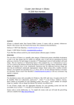
iCluster User Manual v1.03beta
© 2009 Nick Hamilton
License
iCluster is released under Gnu General Public License. It comes with no warranty whatsoever.
Details of the licence may be found in the licence file contained in the distribution.
Software © 2009 Nick Hamilton, [email protected]
Images © 2009 Rohan Teasdale, [email protected]
If you find this software useful in your research please reference the pare (1) below.
Overview
The core idea of iCluster is to spatially place images of fluorescent protein subcellular localisation
is such a way that images that are similar are spatially close. It does this by generating threshold
adjacency statistics for each image to associate a 27 dimensional vector of real numbers with each
image. The set of points in 27 dimensional space is then mapped into 2 or 3 dimensions in such a
way as to preserve the distances between the points as well as is possible. Hence statistically similar
images are spatially close in the visualisation. Statistical tests for difference between image sets
may also be performed, statistically representative images found, along with a number of other
features. The methods are described in [1,2,3]. Here, how to use the principle features of iCluster
are described. Please email Nick Hamilton ([email protected]) with any comments, bug
reports or requests.
Installation
The distribution comes with executables for Windows, Mac OSX and Linux. It requires that Java™
be installed. There are 4 directories: application.* , where ‘*’ is one of linux, windows, macosx,
these contain an executable for each operating system; and images , which contains an example
image set, together with an Image Description File (icluster_description.txt).
To run iCluster, simply enter the appropriate directory for your operating system and start the
executable. Java (version >= 1.5) needs to be installed on the computer.
Source code is in the subdirectory src. To compile the source code you will need the proce55ing
software available from http://proce55ing.org.
Loading an Image Set
To load an image set, the images should be placed in a single directory. Images need to be 8-bit gray
scale in either tiff or png format if statistics are to be generated by iCluster (any png image can be
displayed in iCluster, but statistics generation requires 8-bit gray scale).
The “natural” format of iCluster is png, and tiff format images are automatically converted to png
and saved to disk.
Images may be assigned to classes, for instance treated or untreated, in an image description file
that is contained within the same directory as the image set. Classes are distinguished in the
visualiser by border colours of the images visualised. The format for the file is given at the end of
the document. An example image set together with an image description file
(icluster_description.txt) can be found in the images folder in the distribution.
When iCluster starts, it will automatically read in the last set of images loaded if an image
description file was saved or loaded (see below). If no image set has previously been loaded, when
iCluster starts a file selection window will appear. Selecting an image description file will then load
and display the image set.
Note: If images are missing, the will be displayed in iCluster as a black image with a red X.
Note: If an image set is loaded for the first time, statistics will be automatically generated for that
set if statistics have not been supplied in the image description file. However, the initial placement
of the images in the viewing environment will be random. To find an optimal spatial placement of
the images so that those that are statistically similar are spatially close click on the Sammon Map
check box (see below).
Navigating an Image Set
The following mouse and keyboard controls may be used to navigate around an image set:
View/Hide an Image Class
Left mouse click on the check box for that class
Zoom In/Out
Mouse scroll
Rotate/Translate View
Right mouse drag
Increase/Decrease Image Size
Right mouse + mouse scroll
Increase/Decrease Sphere Size
Left mouse + mouse scroll
View image in detail
Left mouse on image
Select an Image
Right mouse on image
Select a Group of Images
Right Mouse on a central image and drag to select around it
Show/Hide Image Masks
m
Increase/Decrease Image Resolution
+/-
Snapshot
p
Note: for video memory reasons, images are initially viewed at 1/3 of their size. This resolution
may be increased/decreased using +/-. Increasing the resolution too much may lead to memory
problems and the iCluster to crash for large image sets, depending on how much video ram your
computer has. Simililarly, displaying image masks (see below) doubles the amount of video ram
used and may cause problems for large image sets at high resolution. A recent dedicated graphic
card is recommended for use with iCluster.
2D/3D Representation
Image sets may be viewed layed out in 2D or 3D. 3D will typically be better in the sense that the
Sammon mapping (see below) of statistics will better preserve the distance relationships between
statistics for the images. Clicking the Toggle 2D/3D button switches between these representations.
Show Images/Names
The data may either be viewed as a set of images spatially placed by similarity, a set of names of
those images similarly placed, or as a sphere. Clicking on ‘Show Images/Names’ toggles between
these.
Nearest Neighbours
The nearest neighbour to an image is the image that is ‘nearest’ to that image. Nearest may either be
in the sense of the 2D or 3D distance in the viewer, or in the (high dimensional) Euclidean distance
between statistics vectors. Clicking in the ‘Neighbour Join’ will toggle between showing lines
joining nearest neighbours in each of these senses. The number of images whose nearest neighbours
are the same class is also displayed. This gives a sense of how separated the images classes are.
Note: Results may vary according to whether ‘Normalise Statistics’ (below) and ‘Select Statistics’
(above) are set.
Representative Images
A representative image for each class may be shown either using the ‘Rep Images Only’ checkbox
(where images are shown side by side) or ‘Toggle Rep Images’ where representative images are
shown spatially located in 2D or 3D and all other images are hidden. A representative image is
chosen for each class as that image which is nearest to the centroid of the image statistics for that
class. Image size may be increased/decrease in this mode using Right Mouse Button + Scroll Mouse
Button.
Note: Results may vary according to whether ‘Normalise Statistics’ (below) and ‘Select Statistics’
(below) are set.
Add Class
New classes to which images may belong may be added by clicking on the ‘Add Class’ checkbox.
When selected, the user is prompted to enter a name for the class. Press ‘Enter’ to conclude entering
the name. One use for this is to create an ‘Outlier’ class of images which are unusual in some way.
Reclassify Selected
Images that have been selected via right mouse clicking appear with a red tint. Such a set may then
be reclassified to another class by clicking the ‘Reclassify Selected’ checkbox. Once checked, then
user can choose which class to reclassify the images to by clicking on one of the class checkboxes.
Deselect All
All of the selected images may be deselected by clicking the ‘Deselect All’ checkbox.
Selected Images Only
If images have been selected via right mouse clicking, that set of images may be viewed side by
side in 2D by clicking the ‘Selected Images Only’ checkbox. Exit this mode by clicking the
checkbox again. Image size may be increased/decrease in this mode using Right Mouse Button +
Scroll Mouse Button.
Load/Save Data
An image set may be loaded into iCluster by clicking the ‘Load Data’ button. By selecting either a
tiff or png format image in a directory using the file browser that appears, all of the images in that
directory will be loaded into iCluster. However, images so loaded will all be of the ‘Default’ class.
To load images with classes also supplied, a Image Description File (described below) must be in
the same directory as the images. Selecting this file will load the images, their associated classes,
and any statistics or coordinates previously calculated.
An image description file may be saved by clicking on ‘Save Data’ and selecting or creating a file
in the same directory as the images. The next time iCluster is started the last saved Image
Description File will be automatically loaded along with the associated images.
Statistical Testing
Classes of images may be tested against each other to detect if the are statistically different. When
the ‘Statistical Test’ checkbox is clicked, the user is presented with 2 lists of the image classes.
Those image classes selected in the left hand list are then tested against those selected in the right
hand list. Once classes have been selected, click the ‘Finished Selecting Classes’ checkbox, and the
test will start.
The test is for the null hypothesis, that the image sets come from the same population, more
specifically that the mean vectors of the population that the two sets are sample from are the
sample. This is performed using permutation testing as described in [1]. A p-value for the null
hypothesis is returned. The number of repeats to give the p-value may also be selected, though
under most circumstances, the default of 1000 should be sufficient. The Euclidean distance between
the centroids (average statistics vector) of each cluster are also returned.
To exit the Statistical Testing mode, click the ‘Statistical Test’ checkbox.
Note: Results may vary according to whether ‘Normalise Statistics’ (below) and ‘Select Statistics’
(below) are set.
Selecting Statistics
The statistics that are used within iCluster may be selected or deselected by clicking on the ‘Select
Statistics’ checkbox, and then checking/unchecking the listed statistics. It is probably safe to ignore
this unless you want to use iCluster with your own image statistics rather than the automatically
generated threshold adjacency statistics. If you do use your own image statistics within iCluster,
the ability to select/de-select subsets of them may be useful if you wish to examine the effect on
clustering or statistical testing of just using certain of your statistics. See ‘Sample Image
Description File’ below for examples of how to use your own statistics in iCluster.
Image Categories
This is probably not of interest to most users, but iCluster as well as supporting having a class
associated with each image, also supports having categories of classes. For instance the category
‘Subcellular localisation’ might contain the classes ‘Nucleus’, ‘Cytoplasm’, ‘Mitochondria’ and so
on. Most image sets with have just one category containing the classes. However, it is possible to
have other categories of classes, and you can switch between these by clicking on the ‘Change
Image Categories’ checkbox. Another category might be one that contains the classes ‘Punctate’ and
‘Not Punctate’. Hence it is possible to have multiple categories with a class from each category
associated with each image, and then to switch between views of each category. Categories and the
classes within those categories may be defined in the Image Description File, and an example may
be found at the end of this document.
Sammon Mapping
Sammon mapping is the process by which high dimensional statistics vectors are mapped into 2 or 3
dimensions in such a way as to preserve distances between points are well as is possible. Click on
‘Sammon Map Statistics’ to start the process. It is iterative, and so you will see the images fly
around the screen a bit as they find their preferred location. After a period of time the images should
become relatively stable in their location, at which point you may click the checkbox again to stop
the process.
Note: Results may vary according to whether ‘Normalise Statistics’ (below) and ‘Select Statistics’
(above) are set.
Normalising Statistics
Statistics may be normalised, that is for each statistic then mean of the statistic is subtracted and the
result divided by the standard deviation for that statistic. Threshold adjacency statistics are
standardised for the complete image set when first calculated (see below). However, if you wish to
only compare some subset of the complete image set it may be appropriate to normalise the
statistics with regard to that subset. Hence when “Normalise Statistics” is checked, normalisation is
performed with regard to those classes of image that are visible, i.e. their class checkboxes are
selected. Calculations such as representative image selection, high dimensional nearest neighbours,
sammon mapping are then performed with respect to the normalised statistics for the visible images.
In the case of statistical testing, normalisation occurs with regard to those classes of images that
have been selected for comparison.
Threshold adjacency statistics are standardised when first calculated as follows. The normalisation
means and standard deviations of the TAS statistics for the 500 images of 10 subcellular
localisations in Image Set A (described in [1]) were calculated. For any new image set, the TAS as
calculated, and then each statistic is standardised by subtracting the mean and dividing by the
standard deviation for that statistic as calculated for the images for Image Set A. The idea is that
Image Set A provides a reference by which to standardise the statistics for any image set. Hence
when standardised, the Euclidean distances between images statistics vectors are comparable across
any image sets for which the statistics have been standardised. In other words, standardisation
means we have a metric to measure the distance between any images. To use normalised rather than
standardised statistics select the “Normalise Statistics” check box.
Show/Hide Image Masks (‘m’ key)
Statistics are generated for each image by first selecting the cellular regions in the image using a
simple thresholding scheme. The threshold is calculated as m+0.9σ, where m is the modal intensity
in the image, that is the most common intensity value, and σ is the standard deviation of the
intensities in the image. While this produces a reasonable selection for the majority of image
iCluster has been tested on, it may not work in all cases such as when the background is uneven. In
such a case, the result is often an outlier image.
Masks may be viewed by pressing the ‘m’ key while images are being viewed. Press ‘m’ again to
return to viewing the images.
In cases where the automated masking fails completely, the user may supply their own masks for
each image. A mask for an image is an image for which the non-zero intensity pixels select the
regions of interest in the original image. See Sample Image Description File section below for how
to supply a mask image for an image.
Snapshot Images
Pressing ‘p’ will take a snapshot image of the iCluster window. The image is automatically saved to
the directory containing the iCluster executable.
Sample Image Description Files
There are a number of formats which will allow images/classes/statistics to be defined in an iCluster
Image Description File. Essentially the file is plain text with a single line for each image, comma
separated, describing its name, class(es), possibly a mask, possibly user supplied statistics. Hence
exporting an Excel document with appropriate column entries to comma separated format text file
(csv) should produce a correctly formatted file, though the column headings may need to be
removed.
In it’s simplest form, in each line an image name and a class is given, for instance:
010_mitotracker.png,mitochondria
defines the image 010_mitotracker.png to belong to the class ‘mitochondria’.
To supply a mask with each image, a each line might look like:
010_mitotracker.png, 010_mitotracker_mask.png,mitochondria
which is as before, but with ‘010_mitotracker_mask.png’ as the second entry, that being the name of
the mask image associated with the image 010_mitotracker.png. The fact that the second entry is a
mask image is recognized by it’s name terminates in either ‘.png’ or ‘.tif’.
To supply your own statistics for each image, a line might look like
010_mitotracker.png,mitochondria,0.12,0.2,1.45,11.2,2,1.7,-0.3,7.2,-1.4
where the sequence of comma separated numbers are the statistics to use.
Note: Missing values are not supported by iCluster, so ensure all lines contain the same number of
comma separated real numbers.
To have multiple categories for the classes of an image (see Image Categories, above) a list of
classes may be given, instead of a single class. For instance:
010_mitotracker.png,mitochondria,not punctate
might describe the image 010_mitotracker.png as being of mitochondria (in the subcellular
localisation category), but also being of class ‘not punctate’ (in the category punctuate/not
punctate). Similarly, user supplied image statistics might be appended to such an entry.
The most important point for the Image Description File is that every line must have exactly the
same number of comma separated entries. Hence if a mask image is supplied for one image, masks
must be supplied for all. Similarly, each image must have the same number of image statistics (if
supplied), and if there are multiple categories, each containing an image class, then all images must
have entries defining what their class is within that category.
References
1.
2.
3.
Hamilton N., Wang J., Kerr M.C., Teasdale R.D. Statistical and visual differentiation of high
throughput subcellular imaging. BMC Bioinformatics 2009; to appear.
Hamilton N., Pantelic R., Hanson K., Karunaratne S., Teasdale R.D. Fast automated cell
phenotype image classification. BMC Bioinformatics 2007;8:113.
Hamilton N., Teasdale R.D. Visualizing and clustering high throughput sub-cellular
localization imaging BMC Bioinformatics 2008;9:81.
Reference (1) describes the main methods and testing of iCluster. This is the article to reference if
you find iCluster useful in your research.
Reference (2) describes the threshold adjacency statistics that are utilised by iCluster for
visualisation and statistical testing.
Reference (3) describes the method of mapping statistics into 2 or 3 dimensions for visualisation
and an early prototype of iCluster.
iCluster is built using the fantastic proce55ing programming language.
See http://www.processing.org .
Problems
iCluster runs but is sluggish when viewing image
A limiting factor in the visualisation is the graphics card of the computer. A poor graphics card, or
integrated graphics, may produce poor results for larger image sets. A better graphics card will
improve things. Alternatively, the resolution that images are held in memory at may be reduced by
pressing ‘-’ while iCluster is running. This will reduce the amount of memory needed for the
visualisation, but will mean that images are not seen in such detail. iCluster has successfully viewed
a 1000 images of individual cells simultaneously by using a good graphics card on a notebook
computer and reducing the image resolution.
iCluster doesn’t do anything when starting
Try deleting the file config.txt in the directory with the executable. iCluster may be getting confused
about where the default directory/image set is.
Again, large image sets may cause problems dues to memory limitations. Windows Vista seems to
be particularly inefficient in this respect. The Linux distribution of iCluster will readily display
twice the number of images that Vista will on identical hardware.
One work around for this is to reduce the image resolution displayed when iCluster starts. In the
folder containing the executable is the file config.txt. This file contains 3 lines of information, the
default directory of images, the name of the image description file, and a line that reads
iScale=n
where n is an integer. This is a scaling factor used to reduce the image size. For instance, if n=3, the
images will be scaled to 1/3 of their original size. Hence larger image sets may be displayed by
increasing n. Note that this only effect the display of the images, statistics are still calculated on the
raw images.