Download A User's Guide to Reducing Echelle Spectra With IRAF

A User's Guide to Reducing Echelle Spectra With IRAF
Daryl Willmarth
Instrument Support Group
National Optical Astronomy Observatories1
P. O. Box 26732, Tucson, AZ 85726
Jeannette Barnes
Central Computer Services
National Optical Astronomy Observatories1
P. O. Box 26732, Tucson, AZ 85726
May 16, 1994
Echelle spectra are generated by the use of a high angle (typically 63 deg) ruled grating
usually cross-dispersed by a low dispersion grating, grism, or prism. The result is a high
resolution, closely spaced array of side-by-side orders of large spectral coverage. The amount
and nature of the data can be intimidating to observers to reduce and analyze. Fortunately
some powerful tools have been written in IRAF to make this task manageable. This manual
describes the use of these tasks.
Operated by the Association of Universities for Research in Astronomy, Inc. under cooperative agreement
with the National Science Foundation
1
Contents
1 Introduction
2 Overview of Reduction Process
3 Processing Details
3.1
3.2
3.3
3.4
Initial CCD Processing : : : : : : : : : : : : : : : : : : : : : : : : :
Creating a Normalized Flat : : : : : : : : : : : : : : : : : : : : : :
Flat-elding the Data : : : : : : : : : : : : : : : : : : : : : : : : :
Extraction of the Orders|doecslit or apall : : : : : : : : : : : :
3.4.1 Aperture and Background Denition : : : : : : : : : : : : :
3.4.2 Aperture Tracing : : : : : : : : : : : : : : : : : : : : : : : :
3.5 Comparison Identication and Wavelength Solutions|ecidentify
3.6 The Rest of the Story : : : : : : : : : : : : : : : : : : : : : : : : :
3.7 Flux Calibration : : : : : : : : : : : : : : : : : : : : : : : : : : : :
1
1
2
: : : : : :
: : : : : :
: : : : : :
: : : : : :
: : : : : :
: : : : : :
: : : : : :
: : : : : :
: : : : : :
4 Looking at the Reduced Data
4.1 Other Tasks : :
4.2 Image Headers
2
3
8
8
10
14
15
17
17
19
: : : : : : : : : : : : : : : : : : : : : : : : : : : : : : : : : : :
: : : : : : : : : : : : : : : : : : : : : : : : : : : : : : : : : : :
i
19
21
1
Introduction
Echelle spectra are generated by the use of a high angle (typically 63 deg) coarsely ruled
grating usually cross-dispersed by a low dispersion grating, grism, or prism. The result is a
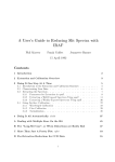
high resolution, closely spaced array of side-by-side orders of large spectral coverage. Figure 1
shows a surface plot of a small section of a typical echelle spectrum viewed parallel to the
orders. In addition to the well dened orders, numerous \cosmic ray" spikes are visible which
will (hopefully) be \cleaned" out of the nal extracted spectra by the tasks described here. As
such, echelles produce excellent formats for two-dimensional arrays such as CCDs. However,
the amount and nature of the data can be intimidating to observers to reduce and analyze.
Fortunately some powerful tools have been written in IRAF to make this task manageable.
This manual describes the use of these tasks, and is a supplement to the following manuals.
A User's Guide to CCD Reductions with IRAF by Philip Massey (hereafter UGCRI)
A User's Guide to Reducing Slit Spectra with IRAF by Massey et al. (hereafter UGRSSI)
The main extraction task, doecslit, has rather lengthy parameter sets, and the document Guide to the Slit Spectra Reduction Task DOECSLIT by Francisco Valdes, should
be at hand.
For users new to IRAF, the document A Beginner's Guide to Using IRAF may be a
good starting point.
Help pages for tasks in the echelle package will also be useful.
This manual assumes that the user is familiar with IRAF, so in this sense it is not a
cookbook. It is also assumed that the user has already made at least one pass with ccdproc
(see UGCRI) to debias and trim the data. Flat-elding requires special considerations and
that is where this manual begins after a summary of the reduction process.
The preliminary reductions are done within the noao.imred.ccdred package; the actual
echelle reductions are done using tasks in the noao.imred.echelle package.
An attempt is made to use dierent font types for IRAF tasks, parameters, and image
names:
a bold font is used for an IRAF task name
an italic font is used for a task parameter
a computer font is used for an image name or an interactive cursor keystroke
2
Overview of Reduction Process
1. Follow the rst six steps as outlined in UGCRI, Section 3.1, to combine zeros and ats,
and to trim and debias the data.
1
Figure 1: Surface plot of a small section of a typical echelle spectrum viewed parallel to the
orders.
2. Create a normalized at from your average at with apatten.
3. Run ccdproc again to at-eld the objects and comps.
4. Extract the data with apall (no wavelength calibration) or doecslit (with wavelength
calibration). In the rst case, wavelength calibration could be done subsequently with
ecidentify, ecreidentity, refspec, setairmass, and dispcor. The output in either
case will be a two dimensional image with as many lines as orders extracted.
3
Processing Details
We now go through the steps listed previously in detail, discussing the individual task parameters.
3.1 Initial CCD Processing
Only a few items will be mentioned here considering the wealth of detail given in UGCRI.
One should implot a few raw biases and ats to check for any uctuation in the overscan
or the lamp. If the overscan is seen to vary by more than an ADU or two from one zero
image to another, one may want to debias and trim the individual images before running
zerocombine or atcombine.
2
If ats are taken in more than one group, say 10 at the beginning and 10 at the end of
the night, there may be a slight image shift on the CCD between the two groups. In this
case it might be preferable to atcombine each group separately to remove cosmic rays and
then run atcombine again without rejection or scaling to combine the group averages into
one nal average at. Otherwise there may be very noisy edges on the average at where the
image shift caused excessive pixel rejection.
One item not discussed in UGCRI is how to x bad columns or pixels by interpolation
with ccdproc. First, one must decide which if any pixels are bad, or are not linear with
at-elding. This may be a bit dicult to determine, but generally if a pixel drops to near
bias level, it will not at-eld. A more empirical method might be used but depends upon
obtaining a couple of groups of ats at dierent exposure levels. After de-biasing the ats and
averaging each group with atcombine, divide one average at by the other with imarith.
Any non-linear pixels should be obvious. One might also be able to determine the faulty
pixels from the data itself after imcopying a test image and at-elding it. Cosmic rays may
confuse the determination however.
After the bad pixels have been identied, create a bad pixel le by identifying them as
rectangular sections, one to a line:
149 149 1 800
250 252 450 800
Here we have a short le identifying the region as column 149 and all rows (lines) of
the CCD as bad. The second line designates the region between columns 250 and 252 and
between lines 450 and 800 as bad. When ccdproc is run on the data, set the parameter xpix
to yes", and the parameter xle to the name of the le you have created, e.g., \badcols".
3.2 Creating a Normalized Flat
Flat-elding is done mainly to remove individual pixel sensitivity variations, chip interference
fringing (if any), and possibly the slowly varying grating blaze function. It is desirable that
the at-elding process does not signicantly change the intensity of the pixels or their relative
values perpendicular to the dispersion. Otherwise, the spatial prole would be altered and
optimal extraction and cosmic ray removal would not be as eective.
We therefore need to normalize the average at by tting its intensity along the dispersion
by a rst or higher order t, while setting all points outside the order aperture to 1. The task
apatten can be used to do this; a typical parameter set is shown in Figure 2. The parameters
are set after examining the particular at to be used. In this case we are using a at from
the echelle/grism setup at the 2.1m coude spectrograph as shown in Figure 3. Apatten
uses parameters from apdefault, apnd, aprecenter, apresize, apedit, and aptrace, so
check these also. Many of these individual tasks have parameters that are redundant with
those in apatten and only the ones specic to that task need be set. The other important
parameter set is the echelle package parameters. Type epar echelle and check the dispaxis
parameter. For orders (roughly) parallel to rows, set dispaxis = 1, and for orders parallel to
3
columns, set dispaxis = 2. You may also want the verbose parameter set to \yes" in order to
see on the screen all the information on the extraction that is sent to the logle.
Notice that even though there is some scattered light present ( 3%), we have background
set to \none" as we are more interested in the variations in the at orders than their exact
level. If your version of IRAF is earlier than V2.10.2, the gain parameter should be set to 1.
A bug in earlier versions causes the output spectrum to be multiplied by the gain. This will
generally not aect the result as cleaning will already have been done during atcombine.
If your version of IRAF is V2.10.2 or later, this should not be a problem.
Running apatten,
apatten Flat
NFlat
will rst enter the aperture editor (Figure 3) where all the relevant apertures can be marked,
if not already, and the aperture widths checked. You may want to set the width of the
apertures using the y key during apedit for a more consistent aperture size than given
by the auto-resize when in the presence of a varying background. When satised with the
aperture selections, type q to enter the aptrace phase where all of the selected apertures can
be traced interactively or at least their traces examined one after another, as described in
UGRSSI, Section 3.3.2.
The ict routine is used here to map closely the position of the aperture along the dispersion axis (Figure 4). If the initial t does not follow the points to the desired closeness
the following parameters can be adjusted:
1. The t order can be increased (:o n, where n is the order number)
2. Deviant points deleted (d with cursor on point)
3. The number of t iterations increased (:niterate n, n=number of iterations)
4. The high and low rejection sigmas (:hi n, :lo n, n=value of cuto)
First time users may wish to review the discussion in UGRSSI, Section 3.3.2.
When the tracing has been nished, another q begins the tting of the 1-dimensional
aperture sum (intensity) along the dispersion to t the general spectral shape of the at eld
light. The t parameters can be adjusted here just like for the aptrace phase. Figure 5
demonstrates how closely the t can be made to the shape of the spectrum. In the far red
fringing will be signicant, and only the envelope of the spectrum can be t. Alternatively,
a rst order legendre or chebyshev polynomial may be used if the shape of the at is to be
preserved.
After running apatten you may want to plot the output image to see the bizarre result. You should see alternating smooth and noisy sections if plotting perpendicular to the
dispersion (as in Figure 6) and a normal looking plot along an order. All values should be
near 1.0. The regions between the orders have been set to 1, and the data inside the aperture
have been normalized to 1 with the large scale uctuations removed. If a rst order function
was t to the light distribution, then the at will have the same shape with an average value
of 1.
4
IRAF
Image Reduction and Analysis Facility
PACKAGE = echelle
TASK = apflatten
input
=
output =
(referen=
(interac=
(find
=
(recente=
(resize =
(edit
=
(trace =
(fittrac=
(flatten=
(fitspec=
Flat List of images to flatten
NFlat List of output flatten images
) List of reference images
yes)
yes)
yes)
yes)
yes)
yes)
yes)
yes)
yes)
Run task interactively?
Find apertures?
Recenter apertures?
Resize apertures?
Edit apertures?
Trace apertures?
Fit traced points interactively?
Flatten spectra?
Fit normalization spectra interactively?
(line
=
(nsum
=
(thresho=
INDEF) Dispersion line
20) Number of dispersion lines to sum
20.) Threshold for flattening spectra
(backgro=
(pfit
=
(clean =
(skybox =
(saturat=
(readnoi=
(gain
=
(lsigma =
(usigma =
none)
fit1d)
no)
1)
INDEF)
6)
2.6)
4.)
4.)
(functio=
(order =
(sample =
(naverag=
(niterat=
(low_rej=
(high_re=
(grow
=
(mode
=
spline3)
1)
*)
1)
3)
3.)
3.)
0.)
ql)
Background to subtract
Profile fitting type (fit1d|fit2d)
Detect and replace bad pixels?
Box car smoothing length for sky
Saturation level
Read out noise sigma (photons)
Photon gain (photons/data number)
Lower rejection threshold
Upper rejection threshold
Fitting function for normalization spectra
Fitting function order
Sample regions
Average or median
Number of rejection iterations
Lower rejection sigma
High upper rejection sigma
Rejection growing radius
5
Figure 2: Typical parameters for the apatten task.
Figure 3: A at from the echelle/grism setup at the 2.1m coude spectrograph with the orders
and apertures marked.
Figure 4: Position of an aperture along the dispersion axis. The line represents the t to the
data points. The tting information is at the top of the plot.
6
Figure 5: Fit along the dispersion of the general spectral shape.
Figure 6: A plot of the output image from apatten perpendicular to the dispersion. The
regions between the orders have been set to 1; the data inside the apertures have been
normalized to 1 with the large scale gradients removed.
7
The last step in preparing the at is to reset the value of CCDMEAN in the header to 1.
This parameter is added to the header during atcombine for subsequent use in ccdproc.
If the value of CCDMEAN is not changed, the object spectra would be multiplied by some
large number and then divided by a at whose value is roughly one resulting in spectra with
counts many times higher than in the original data.
hedit Flat ccdmean 1.0
In IRAF versions V2.10.3 and later apatten will reset CCDMEAN to 1 automatically.
3.3 Flat-elding the Data
Now that we have our normalized at we can proceed to at-elding the spectra with ccdproc.
Trimming, overscan subtraction, and zero subtraction can also be done now if not previously.
With ccdproc parameters set as before,
ccdproc @objects atcor+ at=NFlat
or epar ccdproc to set the parameters. Process the comps in the same manner.
3.4 Extraction of the Orders|doecslit or apall
Generally one will want wavelength scales on the spectra so doecslit is the task to use.
Apall can be used otherwise or if one just wants to do it step-by-step. Doecslit has the
advantage of extracting each comparison spectrum with exactly the same aperture as the
object. Prospective users should read the IRAF document Guide to the Slit Spectra Reduction
Task DOECSLIT by Francisco Valdes. Since apall is just a subset of doecslit, its use will not
be discussed here, but all of the details except wavelength calibration, extinction correction,
and ux calibration are applicable.
A careful examination with implot of a typical object image is useful to determine values
for setting task parameters. These include the base width of the orders, order separation,
maximum signal level, number of orders to be extracted, and scattered light and/or sky
background levels.
There is generally a few percent (compared to order maxima) of scattered light present
in echelle spectra. It is often helpful to average 50{100 rows or columns perpendicular to the
dispersion to see a more accurate view of the nature of the scattered light, as in Figure 7. Here
we nd about 60 ADUs of inter-order light with some structure compared to order maxima
of around 4700 ADUs. We can only assume (conveniently!) the scattered light under an
order is continuous with the inter-order light, and a smooth t between the orders will be
representative. Comparison exposures generally have negligible scattered light.
There is more than one way to subtract scattered light, but the most rigorous method
does it during extraction with doecslit (or apall). This is recommended as only here is the
noise of the background taken into account for cosmic ray cleaning and optimal extraction.
Since the scattered light is highest near the peak intensity of an order, the background noise
8
Figure 7: A plot perpendicular to the dispersion showing the scattered light.
is also higher here; in other words there is a variable background noise level. There are
several methods for subtracting the background within doecslit, and the doecslit guide can
be consulted for details. Here also the distinction can be made between scattered light and
true background from the sky. Sky background will usually not be signicant at the f-ratio
of the coude feed telescope, but could be with the 4-m echelle. If scattered/background light
is to be removed in doecslit, it is important to do a careful job of normalizing the at in
apatten. Fitting a constant to the at to preserve its spectral shape won't do as this at
would change the values of the object spectra compared to the inter-order regions where they
are divided by 1.
A method to subtract scattered light before extraction involves using apscatter where
apertures are dened, sized, and traced. The area between the apertures is then t (with
deviant pixel rejection) perpendicular to the dispersion and then these ts are smoothed in
the orthogonal direction. This is the most time consuming method, and can be shortened by
not smoothing the ts, usually without too much loss of accuracy. This would be similar to
using the task background, except there apertures are not dened. With background the
orders are rejected by setting the parameters low reject and high reject to low values like 1
or 2. Apscatter can also be invoked from within doecslit but the noise values will not be
remembered during weighted extraction.
Typical parameters for doecslit are shown in Figure 8. Note that it has a \nested" parameter set; that is the parameter sparams is actually another parameter set. It can be edited
either by typing :e on that line or with epar sparams. One of the groups of parameters in
9
sparams (see Figure 9) concerns the manner in which the comparison spectra are assigned
to each object spectrum. This is a very exible part of the reductions and can assign and
weight comparison spectra based on the relative time between the object and comparisons,
the position in the sky, or even the date, to mention a few of the possibilities. The default
in doecslit is to run the tasks setjd and setairmass on all spectra to compute and add
the header parameters for the Julian Date (JD), the local Julian Date (LJD), universal time
(UTMIDDLE), and the air mass at the middle of the exposure. This allows the reduction
of more than one night of data by using LJD to group the data with the correct comparison
spectra, and UTMIDDLE to assign the correct spectra within a given night. Using other
criteria for assigning comparison spectra may involve adding new header keywords and computing values for them. The help pages for refspectra describe these options in detail and
give several examples.
What the last paragraph infers is that doecslit is header driven|certain keywords are
expected to be in the image headers. See the help pages for setairmass and setjd for more
information. The image header keyword IMAGETYP must also be present in the image
headers; possible values are \object", \OBJECT", \comp" or \COMPARISON". Data that
are not from NOAO may need to be modied with hedit or asthedit before doecslit will
run properly on the data.
3.4.1 Aperture and Background Denition
Having more or less characterized our images we can now run doecslit:
doecslit @imagelist
It is good practice to review the apertures initially found for the reference object and subsequent images. Occasionally an aperture width will not be wide enough due to asymmetry of
the prole or a local peak. In these cases, the y key or the l and u keys can be used to resize
the aperture. Check for proper numbering of the apertures which should be increasing or
decreasing monotonically. The numbering should also be consistent with any skipped orders;
the desired orders are numbered as if all were there. A useful option can be used by toggling
the all key: if set, other commands will perform the same operation on all the apertures. For
example the y key discussed above would resize all the apertures to the same vertical height
instead of just the aperture near the cursor.
Of the various options available for background subtraction, one will probably want to use
methods that eliminate cosmic rays and take the additional background noise into account.
Global scattered light tting (apscatter) does the former but not the latter. It is also very
slow. The other method involves the denition of background regions on each side of the order
by specifying a buer distance from the edge of each aperture and a range of pixels. The
background regions are set automatically by the program but can be changed interactively
during the background review as discussed below. By using either the \t" or \median"
options of background, cosmic rays can be eliminated and the background noise values will
be taken into account. If sky background is not a factor and just scattered light is present,
boxcar smoothing of the background may be useful. Check the present value while in the
10
IRAF
Image Reduction and Analysis Facility
PACKAGE = echelle
TASK = doecslit
objects =
(apref =
(arcs
=
(arctabl=
(standar=
a0024
a0018)
@comps)
)
)
(readnoi=
(gain
=
(datamax=
(norders=
(width =
6)
2.6)
25000)
24)
7.)
(dispcor=
(extcor =
(fluxcal=
(resize =
(clean =
(trace =
(backgro=
(splot =
(redo
=
(update =
(quicklo=
(batch =
(listonl=
yes)
no)
no)
yes)
yes)
yes)
fit)
yes)
no)
no)
no)
yes)
no)
(sparams=
(mode
=
List of object spectra
Aperture reference spectrum
List of arc spectra
Arc assignment table (optional)
List of standard star spectra
Read out noise sigma (photons)
Photon gain (photons/data number)
Max data value / cosmic ray threshold
Number of orders
Width of profiles (pixels)
Dispersion correct spectra?
Extinction correct spectra?
Flux calibrate spectra?
Resize object apertures?
Detect and replace bad pixels?
Trace object spectra?
Background to subtract
Plot the final spectra?
Redo operations if previously done?
Update spectra if cal data changes?
Approximate quicklook reductions?
Extract objects in batch?
List steps but don't process?
) Algorithm parameters
ql)
Figure 8: Typical Parameters for doecslit.
11
IRAF
Image Reduction and Analysis Facility
PACKAGE = echelle
TASK = sparams
(line
=
(nsum
=
(extras =
(ylevel =
(t_step =
(t_funct=
(t_order=
(t_niter=
(t_low =
(t_high =
INDEF) Default dispersion line
20) Number of dispersion lines to sum
no) Extract sky, sigma, etc.?
-- AUTOMATIC APERTURE RESIZING PARAMETERS -0.05) Fraction of peak or intensity for resizing
-- TRACE PARAMETERS -20) Tracing step
spline3) Trace fitting function
2) Trace fitting function order
3) Trace rejection iterations
3.) Trace lower rejection sigma
3.) Trace upper rejection sigma
(b_funct=
(b_order=
(b_naver=
(b_niter=
(b_low =
(b_high =
(buffer =
(apscat1=
(apscat2=
-- BACKGROUND AND SCATTERED LIGHT PARAMETERS -legendre) Background function
2) Background function order
-5) Background average or median
5) Background rejection iterations
3.) Background lower rejection sigma
1.) Background upper rejection sigma
2.) Buffer distance from apertures
) Fitting parameters across the dispersion
) Fitting parameters along the dispersion
(weights=
(pfit
=
(lsigma =
(usigma =
-- APERTURE EXTRACTION PARAMETERS -variance) Extraction weights (none|variance)
fit1d) Profile fitting algorithm (fit1d|fit2d)
4.) Lower rejection threshold
4.) Upper rejection threshold
Figure 9: Typical parameters for sparams.
12
(coordli=
(match =
(fwidth =
(cradius=
(i_funct=
(i_xorde=
(i_yorde=
(i_niter=
(i_low =
(i_high =
(refit =
-- ARC DISPERSION FUNCTION PARAMETERS -linelists$thar.dat) Line list
0.1) Line list matching limit in Angstroms
3.5) Arc line widths in pixels
5.) Centering radius in pixels
legendre) Echelle coordinate function
3) Order of coordinate function along dispersion
3) Order of coordinate function across dispersion
3) Rejection iterations
3.) Lower rejection sigma
3.) Upper rejection sigma
yes) Refit coordinate function when reidentifying
(select =
(sort
=
(group =
(time
=
(timewra=
-- AUTOMATIC ARC ASSIGNMENT PARAMETERS -interp) Selection method for reference spectra
jd) Sort key
ljd) Group key
no) Is sort key a time?
17.) Time wrap point for time sorting
(lineari=
(log
=
(flux
=
-- DISPERSION CORRECTION PARAMETERS -yes) Linearize (interpolate) spectra?
no) Logarithmic wavelength scale?
yes) Conserve flux?
(bandwid=
(bandsep=
(s_inter=
(s_funct=
(s_order=
(fnu
=
(mode
=
-- SENSITIVITY CALIBRATION PARAMETERS -10.) Bandpass widths
10.) Bandpass separation
yes) Graphic interaction to examine/define bandpasses
spline3) Fitting function
1) Order of sensitivity function
no) Create spectra having units of FNU?
ql)
Figure 9: Typical parameters for sparams|cont.
13
Figure 10: An expanded plot of an echelle order examining the background regions.
apedit stage with :skybox, or set it to the desired value with :skybox 50, for example. If
background subtraction is turned on, check the regions for each order by typing b with the
cursor centered on the order. An expanded plot will be drawn which you may need to expand
vertically (and horizontally) with w and e as in Figure 10 to see the lower levels of the signal
accurately. It might be easiest to start at the order with the largest separation (usually the red
end). The sample region need not omit the order itself since the sigma rejection or medianing
will eliminate the region within the order. The existing sample region can be deleted with z
if necessary, and new ones dened with the s key. If the a(ll) key is set, all other orders will
now have the same size region centered on them. Typing f will t the background and show
the rejected points.
3.4.2 Aperture Tracing
Once the apertures and background regions have been satisfactorily dened, type q to enter
the aperture tracing phase. Here one can interactively t the curve dened by the center of
each order at points along the order specied by the parameters nsum and t step. An initial
aperture trace is displayed, after which the order of the t may be changed (:o n) or points
deleted (d with cursor at point) and the curve ret by typing f. The function type itself may
also be changed (:func chebyshev,legendre,spline1, or spline3) and the curve ret. A
spline3 function has been found to work well for the aperture curves with a dierent number
of pieces for various orders. When a satisfactory t is obtained as in Figure 4, typing q will
display the next order for tting.
14
Figure 11: A plot of the comparison spectrum for the rst order.
3.5 Comparison Identication and Wavelength Solutions|ecidentify
After q is typed for the last aperture trace of the reference spectrum, the rst comparison
image will be extracted based on the apertures just dened for the reference image. The rst
plot will be of the rst aperture of the comparison spectrum (Figure 11). It is assumed that
an appropriate le is specied for the parameter coordlist (\linelist$thar.dat" by default).
The trick now is to identify a few lines in each of an order near the rst, middle, and last
apertures. In other words, you needn't identify lines in all the apertures or necessarily in the
rst aperture, but at least three apertures should have identications. It can be sometimes
dicult to make the initial line identications, and perhaps one of the object spectra with
known lines can help to pin down the rough area. With the help of an appropriate atlas
of the comparison lamp (e.g., A CCD Atlas of Comparison Spectra: Thorium-Argon Hollow
Cathode) set the cursor on a known line, type m (mark) and type in the wavelength. Usually
entering to the nearest tenth of an Angstrom is sucient to match a line in the linelist. Mark
several lines across the order and then move to a new aperture with the j, k or o key. Knowing
the wavelength of one order will enable one to predict wavelengths in other orders with a table
of central order wavelengths such as in the KPNO Coude Spectrograph Manual. Do not type f
(t) until the three or more apertures have had lines marked. Otherwise, the derived t may
not be accurate enough to automatically nd additional lines from the linelist. Occasionally
there will be one or more intense lines in the plot which scale the plot such that few other
lines are distinguishable. In these cases rescaling the plot with w and e will help to see the
lower intensity lines.
15
Figure 12: Initial wavelength tting for an echelle spectrum with residuals versus pixel number
shown. The tting parameters are listed at the top of the plot.
Figure 13: Initial wavelength tting for an echelle spectrum with residuals versus order number shown. This is the same data shown in Figure 12 |just plotted dierently.
16
When sucient lines have been identied, type f to t the default function to the spectrum. Now a plot of deviations from the t vs. pixel number is displayed and interactive
tting may be done. Figure 12 shows an example of this initial t using the default function
and orders. One can see a couple rejected points, probably misidentications, and a noticeable curve indicating a higher order is needed. It may be a little more useful to display the
plot with residual vs. order number (Figure 13) by typing x and o. This will make it easier
to nd a bad identication than just having all the lines displayed as pixel number. Other
options are also shown when typing x. When satised with the initial t, type q to return to
the line identication mode. One can now mark additional lines in other orders to test the
t or type l to locate and mark all the possible lines falling within the acceptance criteria. If
some likely looking candidates are not marked, they may be close blends or the maxfeatures
parameter may not be set to a large enough value. Type f again to enter the two-dimensional
tting routine (Figure 14) and type d to delete points that fall outside of whatever value
you feel is acceptable. The \good" lines generally are pretty tightly clumped about small
residual values. Note the value of the order \oset" shown at the top of the residuals plot;
if the value does not reect the true order of the aperture, it can be adjusted with the o
key. Type q when satised with the t and q again when you are satised with the whole
comparison identication and tting process. Figure 15 shows the residuals from the nal
t with a Legendre function having xorder = 5, and yorder = 6. Order values higher than
these did not improve the t signicantly.
3.6 The Rest of the Story
Unless ux calibration is to be done, the rest of the extraction will be done without interaction.
Then you are queried whether to plot the nal spectra or not (splot = yes). You may wish to
look at least at the rst image to check the results. The line/aperture number will be queried
for, followed by the \band" number. If the parameter extras is \yes", the output image will
be 3 dimensional, with \band" number referring to the following sets of apertures:
band
1
2
3
4
image type
cleaned, weighted, extracted spectra
uncleaned, unweighted spectra
background spectra
estimated sigma spectrum
Band 1 is what we are really after, but the others may be of interest to insure the cleaning
and background subtraction did what we thought it should. The keys ) and # can be used to
move around from order to order, while a dierent band will be used only if % is typed. Since
this poking around is just splot, it will all work the same after the reductions are nished.
3.7 Flux Calibration
Flux Calibration of echelle spectra is problematic due to the short pieces of spectra and
the large bandpasses of most standard star data. An order containing or near a hydrogen
17
Figure 14: A second pass through the tting of the dispersion function for echelle comparison data|more lines have been added to the solution and the tting parameters have been
adjusted.
Figure 15: The nal t.
18
line is especially dicult in the early type stars. Velocity dierences between the object
and standard can change the bandpass enough to cause signicant errors in the presence of
steep line gradients. Unless the observations of the objects and standards are made with the
spectrograph slit at the parallactic angle, signicant throughput dierences will exist between
the extreme orders. In regions of the spectra not containing H-lines however, ux calibration
may be a useful way of attening the rather peaked echelle blaze function. For this purpose
alone though, one may want to consider using the continuum task, as it allows more direct
interaction with the spectrum itself.
Flux calibration in doecslit is accomplished through the tasks standard, sensfunc, and
calibrate. An extinction correction is also applied during the calibrate phase based on
header parameters.
Standard allows an interactive denition of bandpass regions starting with the initial
values found in the sensitivity calibration parameters, or uses those from the calibration le
if bandwith and bandsep are set to \INDEF". Unless the orders span a wavelength interval of
about 100
A or more, it will probably work better to specify the above paramaters as 5 or 10
A.
Since the smallest bandwidths in the standard calibration les are 16A (onedstds$spec16cal),
smaller bandwidth values will allow more points along the order. The standard calibration
data is interpolated to the bandpasses specied or dened graphically. Figure 16 shows an
order with 5
A interpolated bandpasses. If editing of bandpasses is selected, you may add (a)
or delete (d) bandpasses. The nal bandpasses selected for each aperture remain in eect for
subsequent images, so there is no need to edit each time.
After all the bandpasses for each aperture have been dened, a curve tting phase is
entered (sensfunc) where the ux values for each order are t to a smooth curve to relate
system sensitivity to wavelength for each aperture. Figure 17 shows the default plot for an
aperture. Points may be deleted, the tting function type or order changed, and curves may
be shifted (grey shift), to name a few of the options available. See the help pages for this and
the previous task for details.
Finally, the task calibrate applies both an extinction correction and the derived calibration curves for each aperture to produce the nal ux calibrated spectra. This phase is
non-interactive.
4
Looking at the Reduced Data
The splot task can be used to examine the extracted and calibrated spectra. If you are new
to this task read the help page since splot oers many dierent options for plotting and
manipulating the data.
4.1 Other Tasks
Other tasks are also available for extracting, plotting, and combining orders. Some of these
are listed below.
19
Figure 16: A plot of an order with 5
A interpolated bandpasses marked using the task standard.
Figure 17: The interactive phase of the task sensfunc. The units on the left axis are in
magnitudes.
20
bplot
continuum
deredden
dopcor
sarith
scombine
scopy
slist
specplot
specshift
-
Batch plots of spectra
Fit the continuum in spectra
Apply interstellar extinction corrections
Doppler correct spectra
Spectrum arithmetic
Combine spectra
Select and copy apertures in different spectral formats
List spectrum header parameters
Stack and plot multiple spectra
Shift spectral dispersion coordinate systems
4.2 Image Headers
The IRAF image headers are updated throughout the reduction process, and by the time the
echelle reductions have been completed there are a whole spectrum of new keywords added
to the image header. These keywords can vary slightly depending on which version of IRAF
you are using.
A partial image header of a reduced echelle spectrum is presented below, using IRAF
Version 2.10.3. Note that the wavelength information for each order is stored in the WAT
keywords. For a complete description of the headers for spectral data see phelp onedspec.specwcs (IRAF Version 2.10.3 or later) or phelp onedspec.package (in earlier versions).
BANDID1 =
BANDID2 =
BANDID3 =
WCSDIM =
CTYPE1 =
CTYPE2 =
CTYPE3 =
CD1_1
=
CD2_2
=
CD3_3
=
LTM1_1 =
LTM2_2 =
LTM3_3 =
WAT0_001=
WAT1_001=
WAT2_001=
WAT3_001=
WAT2_002=
'spectrum - background none, weights variance, clean no'
'raw - background none, weights none, clean no'
'sigma - background none, weights variance, clean no'
3
'MULTISPE'
'MULTISPE'
'LINEAR '
1.
1.
1.
1.
1.
1.
'system=multispec
'wtype=multispec label=Wavelength units=Angstroms
'wtype=multispec spec1 = "1 113 0 4955.0239257812 0.06515394896268
'wtype=linear
'56 0. 23.22 31.27" spec2 = "2 112 0 4998.9482421875 0.06753599643
21
WAT2_003=
WAT2_004=
DCLOG1 =
DC-FLAG =
STD-FLAG=
EX-FLAG =
CA-FLAG =
BUNIT
=
'3 256 0. 46.09 58.44" spec3 = "3 111 0 5043.6640625 0.06996016949
'2 256 0. 69.28 77.89"
'REFSPEC1 = demostddemoarc.ec'
0
'yes
'
0
0
'erg/cm2/s/A'
22