Download User manual of the (KNMI North Sea Wind) KNW-atlas

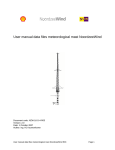
User manual of the (KNMI North Sea Wind) KNW-atlas
Version 8: September 2015
I.L. Wijnant, A . Stepek, M. Savenije and H.W. van den Brink
1
Contents
1 KNMI North Sea Wind (KNW) Atlas ................................................................................................. 3
2 Validation of the KNW-atlas ............................................................................................................. 3
3 KNW-website ................................................................................................................................... 5
3.1 KNW data .................................................................................................................................. 6
3.2 Image browser .......................................................................................................................... 8
4 KNMI Data Center .......................................................................................................................... 10
4.1 KNW (KNMI North Sea Wind) Atlas – END USER PACK ........................................................... 10
4.2 KNW (KNMI North Sea Wind) Atlas – daily 3D model data .................................................... 18
4.3 KNW (KNMI North Sea Wind) Atlas – grid cell time series (NetCDF) ...................................... 18
4.4 KNW (KNMI North Sea Wind) Atlas – grid cell time series (ASCII-CSV) .................................. 19
5 How to use (and not to use) the KNW-atlas .................................................................................. 19
5.1 Diurnal cycle ............................................................................................................................ 19
5.2 Wind maxima over land .......................................................................................................... 21
2
1 KNMI North Sea Wind (KNW) Atlas
The KNW-atlas is a 4D wind atlas based on the ERA-Interim reanalyses dataset which captures 35 years (19792013) of meteorological measurements and generates every 6 hours 3D fields on a horizontal grid of 80 km
which are consistent with these measurements and the laws of physics. This dataset is “downscaled” using the
state-of-the-art weather forecasting model HARMONIE which generates hourly data on a horizontal grid of 2.5
km. The wind speeds were then tuned to match the measurements made at KNMI’s 200 m tall meteorological
mast at Cabauw by increasing the vertical shear of the horizontal wind speed by 15%. The same wind shear
correction factor was applied uniformly throughout the whole KNW-atlas domain and period. The result is a
high resolution dataset of 35 years: the KNW-atlas.
2 Validation of the KNW-atlas
The KNW-atlas has been validated against publicly available wind measurements from three tall offshore wind
masts: OWEZ, FINO1 and MMIJ (Meteorological Mast IJmuiden). The difference between the measured wind
speeds (averaged over periods when the mast measurements were undisturbed by nearby wind parks) and the
KNW values is less than 0.2 m/s for all masts and all measurement heights (figure 1). The validation results
imply that the accuracy of the long term average wind speeds of the KNW atlas is comparable to that of the
measurements (cup and sonic anemometer and LIDAR). The same can be said of the estimates of the once in
10 year extreme wind speeds for heights around wind turbine hub height (figure 2).
Also a first attempt was made to validate the 10 m wind speeds of the KNW-atlas against scatterometer winds
(10 m wind speeds derived from satellite measurements). Compared to the QuikSCAT 25 km product (19992009), the KNW-atlas overestimates the 10 m wind speed for most of the North Sea by less than 0.5 m/s
(figure 3). This is the opposite for the southern part of the North Sea (including the areas Borssele and
Hollandse Kust, designated for wind energy exploitation). Here the KNW-atlas underestimates the 10 m wind
speed by less than 0.5 m/s. Comparing these results to the vertical validation results shows that the validation
at 10 m should not be used to estimate the validity of the KNW winds at the heights relevant for wind energy
purposes.
3
Figure 1: Tall mast validation results (in red KNW-data, in blue cup and in green sonic anemometer
measurements but for MMIJ green means LIDAR).
Figure 2: Tall mast validation of extremes based on measurements (red) and KNW-data (blue) for FINO1 100 m
(left) and MMIJ 90m (right).
The hourly wind speeds in the KNW-dataset represent 40-60 min averages (page 6 TR352).
More information:
•
•
Tall mast validation: http://www.knmi.nl/bibliotheek/knmipubTR/TR352.pdf
Scatterometer validation: http://www.knmi.nl/bibliotheek/knmipubTR/TR353.pdf
4
Figure 3: Scatterometer validation showing average 10 m wind speed difference (bias) between KNW-atlas and
QuikSCAT 25 km product.
3 KNW-website
The wind climatology that is freely available is the KNW-data in the coloured area in figure 4 (referred to as the
“KNW-domain”). The domain’s latitude (roughly from north to south) consists of 188 grid cells and the
domain’s longitude (roughly from east to west) of 170 grid cells. All freely available data can be found on the
KNW website ( http://projects.knmi.nl/knw/ ) 1. KNW-data have also been calculated outside this area
(within the blue frame of figure 4), but these data are not freely available 2.
Figure 4: Left panel: KNW-data have been calculated within the blue frame and are freely available in the
coloured area (the “KNW-domain”). The grid lines indicate the ERA-Interim grid cells (80 by 80 km). Middle
panel: zoomed in on the “KNW-domain”. Right panel: grid cell point locations within the “KNW-domain” (the
layout is the same as the conversion file on the KNW webpage, “GridPointLocations_latlon.csv”, but is upsidedown compared to the maps in the other panels 3.
1
Part of the data is stored in the KNMI Data Centre (KDC) (https://data.knmi.nl/portal/KNMI-DataCentre.html#) but the link to KDC can be
found on the KNW-webpage.
2
It is however possible to make these data available, but only under certain (financial) conditions (for more information:
https://secure.knmi.nl/contact/contact.php).
3
The grid cells (*, 188) are the ones with the highest latitudes (furthest north) and the grid cells with (*, 1) the ones with the lowest
latitude (furthest south). The grid cells (1, *) are the ones with the lowest longitude (furthest west) and (170, *) with the highest longitude
(furthest east ).
5
3.1 KNW data
3.1.1 Basic KNW datasets
KNW-data are stored in the KNMI Data Centre (KDC) and there is a link on the KNW website that gives you
access to KDC. You will find the link to KDC if you select “KNW data” (blue top bar). Once in the KDC, you can
use filter term “KNW” (the “which” filter function) to get to the model data which has been organised into the
three basic datasets. The datasets can be downloaded, but before doing so, please read this manual and make
use of the conversion tables (see links under “Supplementary files”: “Grid point locations” on the website and
described in 3.1.2). You need the conversion tables to translate the coordinates of the location of interest (in
lat/lon or RD-coordinates 4) into the KNW atlas index of the corresponding grid cell.
The three basic datasets contain exactly the same data, but are organised differently or in different formats to
suit different users:
1.
2.
KNW (KNMI North Sea Wind) Atlas – daily 3D 5 model data (KNW-NetCDF-3D): here you will find
NetCDF-files organised in daily files for a fixed domain (the “KNW-domain” described in figure 4). You
can select a day and download all available information for that day (23 values from 01 until 23 UTC
and one from the next day the 00 UTC) in one go. The daily files are available for 5 weather
parameters (temperature, wind speed and direction, pressure and specific humidity) and the units are
included in the file. Each daily file is for a given height above mean sea level (10, 20, 40, 60, 80, 100,
150 and 200m are available). Considering the 3D files for each of the 8 heights together provides a 4D
description of the lower atmosphere. 6. The complete set consists of 35 years of 365/366 days.
KNW (KNMI North Sea Wind) Atlas – grid cell time series (KNW-NetCDF-TS): here you will find
NetCDF-files organised per location (188x170 grid cells with central point in lat/lon) in the
“KNW domain”: you can select a grid cell location 7 and download all available time series (35
years) for that location in one go. Output variables are temperature, wind speed and direction,
3.
pressure and specific humidity on 8 levels (10, 20, 40, 60, 80, 100, 150 and 200m).
KNW (KNMI North Sea Wind) Atlas – grid cell time series (KNW-CSV-TS): the same as in previous set,
but then in ASCII CSV-files.
The basic daily dataset is fairly large: 188x170 (domain size) x 24x365x35 (hourly output over 35 years) x 8
(levels) x 5 (variables) which is in total about 400 x 109numbers (1.5 terabytes). The dataset with ASCII CSV-files
is smaller (0.75 terabytes).
A more detailed description of these datasets can be found in sections 4.2-4.4.
There is a “where” filter function in KDC which is particularly useful if you want to find a timeseries for a
specific location. It enables you to zoom in on the area of interest. Choose “coordinates” and four boxes will
pop up. In these boxes you can fill in the lat/lon coordinates that define the boundaries of your area to the
west (longitude; left box), the east (longitude; right box), the south (latitude; lower box) and the north
(latitude; upper box). E.g. for location Spijkenisse: 4.31 (left) , 4.33 (right) , 51.82 (lower)and 51.84 (upper).
Then click on “FILTER”. In KNW-CVS-TS (3rd row) you will now find 1 page (instead of more than 6000 pages
4
https://nl.wikipedia.org/wiki/Rijksdriehoeksco%C3%B6rdinaten
The NetCDF-files are 3D files (latitude x longitude x time).
6
Latitude x longitude x time x height
7
There are 188x170 grid cells in the “KNW-domain”. For grid cell to lat/lon conversion see: http://www.knmi.nl/samenw/knw/data/
“GridPointLocations_lonlat”.
5
6
without applying the “where” filter) with timeseries for the 3 gridpoints within the area selected. One of them
corresponds best with the location of Spijkenisse: 079-065 (51.84 N, 4.33 E).
3.1.2 Supplementary Files
On the KNW webpage (http://projects.knmi.nl/knw//data/ ) you will also find supplementary files with
information relating to domains, (location) grid points and file listings of the basic datasets to facilitate scriptcontrolled downloading:
•
Maps of the KNW and Borssele domains and the position of the 12 (location) grid points
•
Latitude, longitude and RD-coordinates 8 of all of the KNW grid points (in ASCII-CSV, Excel or NetCDF)
•
File listings of the basic datasets to facilitate script-controlled downloading of the large number of
files
The supplementary files can also be found in the 'END USER PACK' in the KDC
(http://projects.knmi.nl/knw//data/ ).
The links under “Grid point locations” on the website are particularly important. They contain the conversion
tables that you will need to translate the coordinates of the location of interest (in lat/lon or RD-coordinates)
into the KNW atlas index of the corresponding grid cell. The index of the grid cell is the last part of the filename
containing the downloadable time series for that grid cell. In this example, KNW-1.0_H37-ERA_NL-040-180.zip,
the 040 is the part of the grid cell index (with values from 001 to 170) that shows how far east the grid cell lies
and the 180 is the part of the index (001-188) that shows how far north; so this grid cell lies in the far north of
the KNW domain. The conversion tables have 188 rows and 170 columns. The east-west index (corresponding
to longitude and the RD coordinate, x) increases from left to right up to 170 as one would instinctively expect.
The north-south index is the opposite to what one would expect: it increases from top to bottom (up to 188)
with the low values at the top corresponding to the north end of the KNW domain and the high values at the
bottom corresponding to the south. The value in the lat/long conversion table in row 180 and column 040 is
“2.97/54.45” which means 54.45° N, 2.97° E or in minutes (’) and seconds (’’): 54° 27’ 00’’ N, 2° 58’ 12’’ E. In
the RD-coordinate table, the value is “2041/720640” which means x = 2041 meters and y = 720640 meters. If
you open the table in a spreadsheet, such as EXCEL, the spreadsheet might interpret the “/” as a division and
display the result but the coordinates can still be seen if you click on the spreadsheet cell of interest.
8
https://nl.wikipedia.org/wiki/Rijksdriehoeksco%C3%B6rdinaten
7
3.2 Image browser
On the website there is an image browser that can be used to view images of the dedicated KNW datasets.
These dedicated datasets are based on the same information as the basic KNW datasets, but have either been
used to calculate values that are useful for wind energy purposes and/or are extracted for a specific location.
More information concerning the datasets can be found in section 4.1 about the downloadable “END USER
PACK”, which contains these datasets (both the imagery and underlying data).
The images that can be viewed are:
•
•
2D figures for each of the 8 standard heights of the KNW atlas and covering the whole of the “KNWdomain” 9 (average wind speed, Weibull parameters, maximum wind speed, min/max/10%/90% of 11
year running averages and the once in 10, 50 and 100 year extremes)
figures (wind speed distributions, wind roses and time series) and TAB-files for the 12 selected
location grid points 10 listed here below.
The image browser can be found on the KNW-page of the KNMI website (http://projects.knmi.nl/knw/) under
“Image Browser” (blue top bar). The selection scroll bars at the top of the page can be used to select:
1.
The geographical extent of the required information: either the KNW-domain [2D] or a location [1D].
The 12 locations are:
• 6 grid point locations in the “KNW-domain” (figure 5 left) closest to: Cabauw, Europlatform-1,
FINO-1, MMIJ (Meetmast IJmuiden), OWEZ (Windpark Egmond aan Zee) and Lichteiland Goeree
6 grid points in the “Borssele area” (figure 5 right): Borssele point 0 (BORS0), 1 (BORS1), 2 (BORS2), 3 (BORS3),
4 (BORS4) and 5 (BORS5)
2.
3.
4.
The information you require (note that the number of dimensions have to match those of the
geographical extent already selected: [2D] for the area of the KNW-domain and [1D] for a location):
• Average wind speed [2D]
• Weibull shape and scale parameter 11 [2D]
• Maximum wind speed [2D]
• Min/max/10%/90% of 11 year running averages [2D]
• Once in 10, 50 and 100 year extremes [2D]
• TAB-files [1D]
• Wind speed distribution 12 [1D]
• Wind rose [1D]
• Time series of yearly average, smoothed 11-year running average (only available when the period
selected is the 35 year period) and period average wind speeds [1D]
The level: 10, 20, 40, 60, 80, 100, 150 or 200 m height
The period: 35 years (1979-2013) or a subset of 10 years (2004-2013)
9
Figures and underlying aggregated data in folder “2D-domain” in “END USER PACK” described in section 4.1
In folder “GridPoints” in “END USER PACK” described in section 4.1; hourly data for these locations can also be found in this folder.
11
Weibull parameters conform Wieringa/Rijkoord (1983, formula 5.18) with a variable upper limit (the bin that contains the 99th
percentile of the distribution).
12
Plus the Weibull parameters calculated in two different ways: (1) according to Wieringa/Rijkoord (1983, formula 5.18) with a variable
upper limit (the bin that contains the 99th percentile of the distribution) and (2) conform
http://help.emd.dk/knowledgebase/content/WindPRO2.9/03-UK_WindPRO2.9_ENERGY.pdf
10
8
Figure 5: The 2D geographical extent of the dedicated dataset, the KNW-domain (left), and an
example of the 1D geographical extent, the location grid points in the Borssele area (right)
You can select two figures, side-by-side, to facilitate comparing one figure with another.
9
4 KNMI Data Center
The four datasets in KDC 13 are the three basic datasets described in section 3.1.1 and the dedicated dataset
(relevant for most users) in the “END USER PACK” . The “END USER PACK” is described in section 4.1 and the
imagery in the “END USER PACK” can also be viewed with the image browser on the KNW website which is
described in section 3.2. As mentioned earlier in the manual, there is a link to the KDC on the KNW-website
(http://projects.knmi.nl/knw//data/). Use filter term “KNW” to get to the datasets described in the rest of this
chapter.
4.1 KNW (KNMI North Sea Wind) Atlas – END USER PACK
•
•
•
Click on KNW (KNMI North Sea Wind) Atlas – END USER PACK
You can visualise the dataset before downloading (click on “visualize”)
You can download the whole “END USER PACK” in one go (select HTTP or FTP)
The “END USER PACK” contains zip-files grouped in 3 folders (“2D-domain”, “GridPoints” and
“Supplementary”). The zip-files have to be extracted/unpacked before they can be viewed (e.g. with “Paint” or
“Irfanview”) or used for further analysis.
4.1.1 “2D-domain” folder
Figures 6-9 show examples of the imagery contained in the dedicated datasets and the “2D-domain” folder of
the “END USER PACK”. All of the examples are for 100 m height and 1979-2013, but maps for 2004-2013 and
other heights are also available. More precisely, all the 2D images listed in section 3.2 can be found in this
folder. The aggregated data used to make the images can also be found in the “2D-domain” folder.
13
KNMI Data Center
10
Figure 6 Example of the average (left) and maximum (right) wind speed at 100 m height for the whole KNWdomain and the whole 35 year period
Figure 6 shows examples of the average and maximum wind speed at 100 m height for the whole period of the
KNW Atlas. Maps of the period minimum wind speed are also available. Note that the wind speed legend is
different for the average and the maximum wind speed. The maximum wind speed is the highest value of the
hourly average wind speed in the 35 years that the KNW dataset covers. The maximum values over sea are an
accurate representation of the wind speed on the hour and day when the maximum occurred in reality. The
high values over Groningen and the Dollard area are less accurate. They are from an extreme event that the
KNW atlas (read HARMONIE) produced for the 1st of August 1983. This value is theoretically possible (once in
10.000 year event), but the wind speeds measured on that day were significantly lower (see chapter 5.2).
11
Figure 7 Example of the scale (left) and shape (right) parameter (right) of the Weibull distribution at 100 m
height for the whole KNW-domain and the whole 35 year period
Weibull parameters (examples in figure 7) have been calculated conform Wieringa/Rijkoord (1983, formula
5.18) with a variable upper limit (0.5 m/s bins from 4 m/s up to, but not including, the bin where the
cumulative distribution equals or exceeds 0.99).
12
Figure 8 Example of the minimum (upper left), maximum (upper right), 10th percentile (bottom left) and 90th
percentile 14 (bottom right) of the 11-year running average wind speed at 100 m height for the whole KNWdomain and the 35 year period
14
Calculated with climate data operators.
13
Figure 9 Example of the once in 10 year (left) and once in 100 year (right) extreme wind speed for the whole
KNW-domain based on a Gumbel fit of the annual maxima of 1979-2013. Once in 50 year extreme is not
shown.
The parameters of the Gumbel distribution are determined by Maximum Likelihood from the annual maxima.
The return value RV for a given return period T is given by:
𝑅𝑅 = 𝜇 + 𝜎 ∙ ln(𝑇)
Here, μ is the location parameter, and σ the scale parameter of the Gumbel distribution.
4.1.2 “Grid points” folder
Figures 10-13 illustrate the images and aggregated data available in the “Grid points” folder for the 12 selected
grid points, using location Meetmast IJmuiden (MMIJ) and the period 1979-2013 as an example. The images
and aggregates are available for both 1979-2013 and 2004-2013 and for other heights. More precisely, all the
1D images and TAB-files listed in section 3.2 can be found in this folder.
Figure 10 is an example of a TAB-file, in this case for the KNW grid point horizontally closest to Meetmast
IJmuiden (MMIJ) at a height of 100 m (the values at the grid points directly above and below this height are
linearly interpolated) and for the whole 35 year period. It shows the wind speed frequency distribution for 12
wind direction sectors and for all wind directions together. It also shows the frequency distribution of the wind
direction sectors for 30 wind speed “bins” of 1 m/s. The last column shows values for all wind directions
combined, the other columns show values for 30 degree wind direction “bins”. The first row lists the average
14
wind speed [m/s], the second row the Weibull Scale parameter A [m/s] - which is a related to the average wind
speed but not exactly the same - and the third row the Weibull Shape parameter k [-]. The value for “% ff>=0”
gives per wind direction sector of 30 degrees the frequency of occurrence of these wind directions considering
all wind speeds. The total number of data used here is 306816 (N) which is roughly speaking 35 years x 365
days x 24 hours. In the remaining rows the TAB-file shows how the data is distributed over the wind speed and
wind direction “bins”. The values in these bins are in units of 0.1 percent of all the data for the relevant wind
direction sector (so 10 means 1%). In the last column we see the frequency of occurrence of wind speeds
(irrespective of wind direction) per bin in percent (so not in 0.1 percent). Figure 10 shows that, according to
the KNW-atlas, the prevailing wind direction at MMIJ at 100 m height is SSW (195-225 degrees) because the
highest figure in the fourth row (“% ff>=0”) is 15.2 %. Similarly the prevailing wind speed is 9-10 m/s (5
Beaufort) because 8.1 % is the highest figure in the column on the far right.
So you can use the table to find the prevailing wind direction or the prevailing wind speed, but you cannot use
the table to find the most prevailing combination of wind direction and wind speed. It would appear to be NNE
(15-45 degrees) and 8-9 m/s (between 4 and 5 Beaufort) because the highest number in the lower part of the
table is 104 (=10.4%), but this interpretation is incorrect. This is because the percentage in the bin is relative to
the total number of data for the wind direction sector NNE and the wind blows from these directions much
less often than from SSW. The highest value in the SSW column (7.5%) represents more data than the 10.4% of
data from NNE. One glance at the wind rose of figure 12 makes this clear, where the percentages are relative
to all the data and not just to those of a given wind direction sector. The fact that 10.4% is the highest value is
also partly because NNE has the lowest average wind speed so the occurrences are forced to fit into fewer
wind speed bins than for wind direction sectors with higher wind speeds.
Figure 10: Example of a TAB-file (Meetmast IJmuiden at 100 m height).
15
The wind speed distribution in figure 11 is based on the TAB-file shown in figure 10. All wind directions have
been included, so just as in the last column of figure 10 we see a prevailing wind speed between 9 and 10 m/s.
The Weibull parameters are calculated in two different ways: (1) according to Wieringa/Rijkoord (1983,
formula 5.18) with a variable upper limit (the bin that contains the 99 percentile of the distribution) and (2)
conform http://help.emd.dk/knowledgebase/content/WindPRO2.9/03-UK_WindPRO2.9_ENERGY.pdf. The 1
m/s “bins” of figure 11 were chosen to make the graph clearer, but smaller bins of 0.5 m/s were used when
calculating the Weibull parameters.
Figure 11: Example of a wind speed distribution (Meetmast IJmuiden at 100 m height).
Again we show the KNW-climatology for grid cell MMIJ at 100 m height that was presented in figures 10 and
11, but this time in the form of a wind rose (figure 12). The wind direction “bins” are the same as in the TABfile (figure 10), but the wind speed “bins” are chosen differently (3 m/s instead of 1 m/s “bins”) to make the
graph clearer. The percentage of the data shown by the various colours is also different: in this case they are
percentages relative to the total number of data and not just the data with wind directions in the given wind
direction sector. These aggregates have not been included in the TAB-file. It would be difficult to misinterpret
this figure (as opposed to figure 10) and conclude that the most prevalent combination of wind speed and
wind direction was one of the NNE bins.
16
Figure 12: Example of a wind rose (Meetmast IJmuiden at 100 m height).
For all selected grid points (the 6 Borssele points and 6 reference points in the KNW-domain described in
section 3.2), time series of the yearly averages and smoothed 11 year running means are provided (obviously
the 11 year running mean can only be calculated for the 35-year period: the 10-year period is too short) as well
as the average over the whole period. Figure 13 shows an example for MMIJ at 100 m height for the whole 35year period. The aggregated wind speeds shown on the graph are not available in the “END USER PACK” but
the hourly data is. In the basic datasets, described in paragraph 3.3.3 and 3.3.4, hourly time series are available
for all of the grid points in the KNW-domain.
Figure 13: Example of a wind speed time series (Meetmast IJmuiden at 100 m height). Yearly averages in black,
smoothed 11 year running mean in blue and the average over the whole period in red.
17
4.2 KNW (KNMI North Sea Wind) Atlas – daily 3D model data
•
•
•
•
•
Click on KNW (KNMI North Sea Wind) Atlas - daily 3D model data
Click on “visualize” if you want to visualise the dataset before downloading
Select a day within the 35-year period (from 1979-01-01 01:00 to 2014-01-01 00:00). The most recent
days are at the top of the list and you can scroll down using the “page” button. The selected dataset
consists of 24 hourly data from 01:00 to 00:00 UTC on the day you have selected for every grid cell in
the KNW domain (188 x 170 x 8).
You can download the selected day files (select HTTP or FTP)
Once the netCDF file is opened 15 you will find a list of (sub) datasets:
o where, in the name, D is wind direction, F is wind speed, P is pressure, Q is specific humidity
and T is temperature. The numbers indicate the height above mean sea level (10, 20, 40, 60,
80, 100, 150 or 200 m height). Each of these datasets represents 24 2D maps of a weather
parameter at a given height; one map for each hour of the selected day.
o where structural information is stored, e.g. “time” shows that data are stored from 01 UTC
until 00 UTC each day; “lat” and “lon” show respectively the latitude and longitude of the
188 x 170 grid cells.
4.3 KNW (KNMI North Sea Wind) Atlas – grid cell time series (NetCDF)
•
•
•
•
•
15
16
Click on KNW (KNMI North Sea Wind) Atlas – grid cell time series (KNW-netCDF-TS)
You can visualise the dataset before downloading (click on “visualize”)
Select the grid cell of interest from the horizontal grid of the KNW-domain. The grid index is included
in the name of the netCDF file, e.g. KNW-1.0_H37-ERA_NL-001-002.nc, where 001 is the longitude
index (001-170) and 002 is the latitude index (001-188). The lowest index values are at the top of the
list and you can scroll down using the “page” button above the list of files. The selected dataset
consists of hourly data (see the 5 weather parameters and 8 heights listed in the next bullet point) for
the period 1979-2013.
You can download the selected grid cell files (select HTTP or FTP)
Once the netCDF file is opened 16 you will find a list of (sub) datasets:
o where, in the name, D is wind direction, F is wind speed, P is pressure, Q is humidity and T is
temperature. The numbers indicate the height above mean sea level (10, 20, 40, 60, 80, 100,
150 or 200 m height). Each of these datasets represents a single time series of a given
weather parameter at a given height.
o where structural information is stored, e.g. “time” shows that data are stored for 306816
hours from 19790101 at 01 UTC up to and including 20140101 at 00 UTC; “lat” and “lon”
show respectively the latitude and longitude of the grid cell.
For software that you can use to manipulate or display NetCDF-files we refer to www.unidata.ucar.edu
For software that you can use to manipulate or display NetCDF-files we refer to www.unidata.ucar.edu
18
Figure 14: An example of a grid cell time series (nearest grid cell to MMIJ) showing the hourly average wind
speed.
4.4 KNW (KNMI North Sea Wind) Atlas – grid cell time series (ASCII-CSV)
The time series that can be downloaded here contain the same information as those of the previous section.
The main difference is the format of the files and that there are individual files for each weather parameter
and height combination. ASCII CSV files do not require separate sub datasets with structural information
concerning time and locations.
5 How to use (and not to use) the KNW-atlas
The wind speed of the KNW-atlas has been validated against measured averages ranging from one year
(OWEZ) to ten years (QuikScat). Based on this validation, the conclusion can be drawn that the quality of the
KNW-atlas is high at these time scales (less than 0.5 m/s at 10 m and less than 0.2 m/s at greater heights) and,
moreover, comparable to climatology based on measurements for heights above 10 m.
5.1 Diurnal cycle
The KNW-atlas has not been thoroughly validated on shorter timescales (months, days or hours). However,
figure 15 shows a comparison with measurements for two periods of 10 days with both extremely high and
low winds. The KNW and measured time series match quite well. So even on the time scale of 1 hour the KNW
19
wind speed can be used effectively. The high winds from 10-20 January are from different directions (10-12010 easterly, 13-1-2010 southeasterly and 16-1-2010 southerly).
Figure 15: Comparison of measured hourly average wind speeds (blue) and KNW-values (red) for FINO1 at 100
m height from 10 until 20 January 2010. Wind speeds in m/s.
However, there is a problem present in the time series of figure 15 but it is so small that it is barely visible.
Because of the way the KNW-atlas was constructed, the atlas reconstructs the diurnal variation of wind speeds
less accurately than wind speeds averaged over longer periods. The saw-tooth patterns exhibited by the
graphs of the diurnal variation (example in figure 16), are an artefact of the KNW-atlas. This is caused by the
initialisation of the HARMONIE weather forecasting model at 0, 06, 12 and 18 UTC with the lower ERA-Interim
wind speeds. It takes a number of hours into the forecast before HARMONIE develops more realistic, smaller
structures and higher wind speeds than ERA-Interim is capable of. The forecast hours included in the wind
atlas dataset (hours 1-6, with 0 being the initialisation time) were chosen to optimally match measurements
made at KNMI measurement sites at the meteorological standard height of 10 m. Since then however, Wijnant
et al (2015) have shown that using longer forecast lead times would probably improve agreement with
satellite-based measurements of the 10 m wind above the North Sea. There is obviously a limit to this because
there is a limit to how far ahead you can forecast accurately. So KNW winds should not be used for diurnal
analysis unless care is taken to account for this artefact.
An example where the KNW atlas wind speeds can still be used in an application involving diurnal analysis
despite the saw-tooth pattern is for the calculation of wind turbine noise. Since 2004, European legislation
requires distinguishing between 3 periods of the day: daytime (07-19 LT), evening (19-23 LT) and night (23-07
LT) 17. These are then combined into one formula for the year average noise level caused by a wind turbine or
park (Lden: Level day, evening, night), which is:
The 3 L’s are based on the frequency distributions of the wind speed for the corresponding 3 periods of the
day.
17
Source https://nl.wikipedia.org/wiki/Lden. In the Netherlands the difference between UTC and local time is 1 hour in the winter and 2
hours in the summer (e.g. 18 UTC = 19 LT in the winter and 20 LT in the summer).
20
Figure 16: Diurnal analyses at of the hourly average wind speed at 60 m height at MMIJ. Measurements (blue)
and KNW-atlas (red). KNW-atlas contains the +1 to +6 HARMONIE forecasts (+ shear correction), initialised
every 6 hours (00, 06, 12 and 18 UTC) using ERA-Interim values.
To see if the KNW atlas wind speeds can be used for this purpose whilst retaining the levels of accuracy shown
for analyses of longer periods, one has to compare the periods used to the periods of the saw-tooth pattern.
•
•
•
The daytime period in winter covers exactly 2 successive saw-tooth periods, so the accuracy of the
frequency distribution should be very similar to the accuracy of the KNW atlas as verified in earlier
reports. The change due to summertime should be small.
The evening period is slightly shorter than 1 saw-tooth period and the missing forecast hour in
summer is the fourth, which is close to the measured wind speed because it is one of the middle
hours in the saw-tooth period. In winter the fifth hour is missing so the frequency distribution will
have a larger bias to lower wind speeds than when the KNW wind speeds are analysed for longer
periods.
The night period is slightly longer than the saw-tooth period and the consequences are unimportant
because the extra forecast hours are the third, fourth and fifth. However in the winter the extra
forecast hours are the fourth, fifth and sixth so the frequency distribution will have a larger bias to
higher wind speeds than when the KNW wind speeds are analysed for longer periods.
So the KNW atlas can be used for diurnally dependent wind turbine noise level calculations for all periods of
the day and in all seasons without loss of accuracy except for the winter evenings and nights. The accuracy of
the KNW atlas wind speeds should be verified for these periods before using them for wind turbine noise level
calculations.
5.2 Wind maxima over land
The high values for the maximum hourly average wind speed at 100 m height over Groningen and the Dollard
area in figure 6 (repeated in figure 17 top) are from an extreme event that the KNW atlas (read HARMONIE)
produced for the 1st of August 1983 06 UTC (with a chance of happening of once in 10.000 years). There are
few, if any, measurements at 100 m from this period to compare the KNW data to, so we use measurements at
the standard meteorological wind measurement height of 10 m for the comparison. The measured wind
speeds are unusually strong but cannot be classified as extreme because they occur more than once a year.
The KNW maximum hourly average wind speeds at 10 m height (figure 17 below) are extreme and significantly
21
higher than the ones measured that day. Where the KNW atlas produces a daily maximum of the hourly
average wind speeds of more than 18 m/s between 05 and 06 UTC, the nearest KNMI measurement site Eelde
(280) measures a daily maximum of “only” 11.8 m/s between 11 and 12 UTC (which is much more realistic
time of day for the maximum wind speed in convective weather situations than between 05 and 06 UTC).
Deelen (275) and Beek (380) register higher values for the daily maximum than Eelde (respectively 12.3 m/s
and 13.9 m/s, both between 08 and 09 UTC), but still significantly lower than the KNW maxima.
We want to emphasise here that the maximum values in the KNW atlas above land are possible (the 100 m
maxima near Groningen occur once in 10.000 years), but may be much higher than what has actually been
measured in the past 35 years. The maximum values over sea areas are much more accurate.
Figure 17: Example of the maximum wind speed at 100 m height (top) and at 10 m height (below) for the whole
KNW-domain and the whole period of 35 years.
22