1
SwanOne User Manual SwanOne User Manual Version of 18-3-2015 1 SwanOne User Manual Table of Contents 1. 2. 3. Introduction....................................................................................................................................... 3 Installation ........................................................................................................................................ 3 Starting with SwanOne ..................................................................................................................... 3 3.1. File – New .................................................................................................................................. 3 4. Input data ......................................................................................................................................... 4 4.1. Input – Bottom Profile ................................................................................................................ 4 4.2. Input – Define Current ............................................................................................................... 5 4.3. Input – Boundary Conditions ..................................................................................................... 6 4.4. Input – Output Locations ........................................................................................................... 7 5. Computing ........................................................................................................................................ 8 6. Creating Output ................................................................................................................................ 8 6.1. General ...................................................................................................................................... 8 6.2. Output – Rays Plot .................................................................................................................... 9 6.3. Output – Spectrum plots .......................................................................................................... 10 6.4. Output – Prints ......................................................................................................................... 11 7. Help ................................................................................................................................................ 11 7.1. About ....................................................................................................................................... 12 7.2. Liability ..................................................................................................................................... 12 Annex 1 Output Parameters .................................................................................................................. 13 Annex 2 Swan Spectral File .................................................................................................................. 15 Version of 18-3-2015 2 SwanOne User Manual Introduction ... 1. Installation SwanOne is developed in MatLab, and is delivered as an executable. However, you can run the SwanOne executable only when the MatLab Runtime Component is installed on your computer. For this version you need version 7.7. You can download this package from the SwanOne download page. After downloading run MCRinstaller77.exe. Check the correct installation; you should have a folder: C:\Program Files\MATLAB\MATLAB Component Runtime/v77 Download SwanOne.zip from the SwanOne download page and extract all files in a convenient folder, e.g. C:\Program Files\SwanOne. You can make for your convenience a shortcut to SwanOne.exe and place this shortcut on your desktop or in the folder C:\Documents and Settings\...\Start Menu\Programs Startup SwanOne by double click on SwanOne.Exe. In the background you will see a black screen showing the logfile. This screen is not relevant for you. The main screen of SwanOne will open. 2. Starting with SwanOne 2.1. File – New You may define any folder to be used as the SwanOne working directory. In this folder you should have placed your input data files and also your output will be written into this folder. By default SwanOne will use the folder in which the program resides, but usually that is not a very handy place. If you want to place all SwanOne data in a dedicated folder, you have to create this folder; you may create this folder in SwanOne, but it is handier to create it on beforehand. As an example in this manual, the working directory is E:\SwanCases. In this folder a subfolder with the name E:\SwanCases\profiles has been created with the various input files. Start SwanOne. Two windows will open. One window has a black background and is the Matlab logfile window. You don’t have to pay any attention to that window. The other window is normal SwanOne window. Only the tab “File” is active. Click on “new” (the other option is “exit”, which is not relevant at this moment). Now you get the “new project” screen. In this version of SwanOne it is not yet possible to open existing files, so you start a new project. In the box “Folder Name” you type the name of the SwanOne data folder, or you select this folder with the “Browse” button. Then you type in the box “Project Name” the name of your specific computation. In the example below the case is called Case1. Version of 18-3-2015 3 SwanOne User Manual Continue via the “OK” button. 3. Input data 3.1. Input – Bottom Profile SwanOne requires a bottom profile. This is an ASCII file (e.g. a txt file, made with Notepad). In this file you place water depth information. The file should consist of two columns, separated by (at least) one space. In the first column the distance is given in m from your deep water starting point, in the second depth is given in m below Chart Datum. Depth should be entered as a negative value. The distances are not necessarily equidistant; values can be entered as real values (use a point as decimal separator). You have to place this depth file in a folder. In this example all profiles are placed in the folder E:\SwanCases\profiles. You may have different files with bottom profiles in this folder. You may type in the folder name, or use the “Load File” button to go to this file. The profile will be displayed in a small figure. Version of 18-3-2015 4 SwanOne User Manual At his moment only input as an XZ file is possible. Also the option to edit the depth file in SwanOne is not yet operational. So editing of the depth file should be done outside SwanOne, e.g. with Notepad. Also you have to enter the orientation of your coastline. The direction you should give here is the orientation with respect to north, when looking from the sea to the land. The “Display” button allows you to see your selected option. In this example a profile of the Dutch coast near Petten is selected. Alpha is the direction of the profile with respect to a viewing direction o from north. For this example a value of alpha = 200 has been selected. The profile has to be perpendicular to the coastline. Save your settings by clicking on the “save” button. Saving the file with the “save” button will automatically close the screen. However you can also close without saving by clicking on “close”. Note: when clicking on “save” without loading the bottom-file, the program will stop with a warning message. 3.2. Input – Define Current In case you do not want to include currents you have to select in this screen the option “No Current” and save. In case you do not select anything, SwanOne will not run. Usually the effect of currents is small, therefore as startup it is recommended not to include currents. However do not forget in that case to save the “No Current” option. When you want to include currents, you have to make a current input file. This file should consist of three columns, separated by at least one space. In the first column should be the distance as used in the depth profile. In the second column is the velocity perpendicular to the profile, in the third column is the velocity in the same direction as the profile. Version of 18-3-2015 5 SwanOne User Manual The velocities are given in m/s. The distances between the points can be arbitrarily. SwanOne will interpolate linearly between the points. For orientation is referred to the small sketch above. The datafile with currents can be made with Notepad, and can be stored in the same folder as the depth profiles. Outside the defined areas the velocity is assumed to be zero. 3.3. Input – Boundary Conditions In this screen the wave boundary conditions for the deep water edge are set. You may either define an arbitrary spectrum via a file or define input parameters. For beginning users it is recommended to use Parameters. You may define your input spectrum via parameters by entering a deep water waveheight (Hm0) and a deep water peak period (T p). SwanOne converts these data to a Jonswap spectrum with a peak enhancement -5 factor = 3 and an f spectral tail. Also the wave direction has been set. Direction is with respect to north. o In this example the wave direction is set to 30 . Note: In fact you are not defining the wave height at the boundary, but you define the amount of wave energy entering your model. Because of this, you may see a deviation between the wave height defined by you at the boundary and the calculated wave height in point 1. For further info, see Appendix 1 to this manual. In a more advanced mode, you may define the input spectrum at the boundary. In that case select “SWAN 1-D Spectrum”, load a spectrum file and save. The spectrum file has to have a specific format. As input file you may use an output file of SwanOne. This allows you to nest models, e.g. a course grid model from very deep water to shallow water, and a fine grid from shallow water to the coastline. The output file with extension SP1 from the course SwanOne model can be used directly as input file for the fine grid model. You may also make an input file yourself using Notepad. This has to be done quite accurate, because SwanOne does not tolerate (minor) typing errors. In Appendix 2 the SWAN spectrum file is discussed in more detail. In this screen also a deviation can be set of the waterlevel. It is recommended to enter the depth in the bottom profile with respect to Chart Datum, so at this point you can set the waterlevel with respect to Chart Datum. In the example a waterlevel of CD+1 is selected. In the box you may also select if you want Swan to include a waterlevel rise due to wave set-up. In the lower right box you may set the wind speed and wind direction. Wind speed should be set in m/s, wind direction wit respect to North. In o this example the wind direction is 5 . Beaufort 1 2 3 4 5 6 Version of 18-3-2015 m/s 1.5 3.3 5.5 8.0 10.8 13.9 Beaufort 7 8 9 10 11 12 m/s 17.2 20.7 24.5 28.4 32.6 >33 6 SwanOne User Manual With the “display” button you can visualise all input directions. Close this window after use. In case too many of these windows are open at the same moment, SwanOne will stop and provide an error message. After entering your data you have to save the information by clicking the “save” button; the screen will be closed. You can close without saving by clicking on the “cancel” button. 3.4. Input – Output Locations SwanOne provides a number of spectral parameters at any point of the bottom profile. However, a full spectrum is only provided at pre-selected locations. In this screen you may enter the locations in the 8 boxes. No more than 8 output locations are possible in the present version of SwanOne. In this example a spectrum is selected at the deep water boundary (input spectrum), on the intermediate shelf and a number very near to the coast. When a value is selected outside the profile (in this example at 3700m) the plotted profile will be horizontal. Save the data by clicking on the “save” button; the screen closes. You may also close without saving by clicking on the close ’button. The “Display” button gives markers on the screen where the spectra are calculated. Version of 18-3-2015 7 SwanOne User Manual Note: You have to select at least one output location, otherwise the program terminates with an error message. 4. Computing By clicking on the computing tab, the computation screen opens. It shows default values for the step size and for the number of steps. These values can be changed to make the computation more accurate (and more slow). After changing one value (either dx or Number of Steps) press “Edit” to compute the other value. Start the computation with the start button. At this moment SwanOne calls Swan.exe to make the computation. This may take some time, depending on the performance of your computer. 5. Creating Output 5.1. General The basic information is written in a subfolder of the SwanOne cases folder, in this example the name of the subfolder was defined as “Case1” (see explanation in the chapter “Input”). This folder may contain the following files: MAT PRT SWN TAB _bot.DAT Internal Swan-file, not readable Swan report file Swan input file for the batch process Standard outputfile of Swan Expanded bottom profile file for internal use of Swan _pointX.SP1 One dimensional spectrumfile for output point X _pointX.SP2 Two dimensional spectrumfile for output point X _Table.TAB Output file as produced by the Tablse command of SwanOne All files can be read with Notepad. However, it might be useful to open files in Excel. In that case you have to change text to columns. Select column A in Excel and open “Text to Columns” in the “Data” tab of Excel. Select “delimited” and “space” as the delimiter. Version of 18-3-2015 8 SwanOne User Manual Note: in case you have European settings for numbers (i.e. 0,23 instead of 0.23) in Excel, you first have to change all points in comma’s. Do this with the “replace all” command in Excel, before you apply the “Text to columns” command 5.2. Output – Rays Plot After clicking on “Rays Plot” the ray plotting windows open. First you have to define the graphs you are interested in. Click for that purpose on “define graphs”. The screen “define ray-plot” opens. You may select up to four graphs in one screen. View1 is default on Hm0. Mark one of the parameters. In case you want more plots, click on View2 and select your second parameter. In this example the Hm0, the Tm-1,0 the direction and the depth are selected for the subsequent views. After clicking on “done”, the basic screen is opened with the requested graphs. With the “options” button you may change the scales; for example to plot a detail of the last 500 m of the computation, set the horizontal scale from 2500 to 3000 m. Version of 18-3-2015 9 SwanOne User Manual The options function is also very handy when comparing two parameters with the same unit, e.g. comparing Tm and Tm-1,0. Then the vertical scales can be made identical. See example. Version of 18-3-2015 10 SwanOne User Manual 5.3. Output – Spectrum plots Clicking on “spectrum plots” opens the spectrum plot window. Click on “define graphs” to select the spectra. At this moment only 1D spectra are possible. Up to 4 spectra can be plotted in one screen. Only one spectrum can be selected per view. The option not to plot gridlines is not active in this view. 5.4. Output – Prints The print tab opens a menu where you can select parameters to be printed in a table. When you select the option of printing to file, the file appears in the Case folder (in this example SwanCases/Case1; see also Output-General, above). Printing direct to a printer is not yet possible. For further info regarding the standard outputfiles of Swan is referred to the Swan documentation (http://www.swan.tudelft.nl/online_doc/swanuse/node50.html). The SP1 file gives the (one dimensional) energy spectrum, while the SP2 file gives the directional spectrum Version of 18-3-2015 11 SwanOne User Manual 6. Help The help option is not yet implemented. Use this manual for help 6.1. About In the “about” screen (which will be a subscreen of Help) you find information regarding the version of SwanOne and the embedded version of Swan. This manual is written for SwanOne version 0.01 and this version is using Swan 40.72. SwanOne is developed by TU Delft, section Hydraulic Engineering. It is based on a Visual Basic package originally developed by Alkyon under contract for the Netherlands Ministry of Public works. SwanOne is written in MatLab by Sepehr Eslami Arab under the guidance of Henk Jan Verhagen (section Hydraulic Engineering) and Gerbrant van Vledder (section Fluid Mechanics). 6.2. Liability The computer program SwanOne has been initiated and written by Delft University of Technology. The program has been thoroughly checked in accordance with the latest developments in hydraulic engineering. Whilst every endeavour was made to ensure a program free of errors, the collaborators do not warrant, guarantee or make any representation regarding the use, availability, reliability, or the results of the use of the software. This includes the accuracy, correctness or completeness of any elements of SwanOne or of information provided within SwanOne. By using this program, the user agrees and accepts the statements below: Delft University of Technology and everyone who has collaborated with this program do not accept any liability in any event. This includes direct, indirect, special, punitive, incidental or consequential damages (such as loss of income, company breakdown, damage to reputation and missing orders) as a consequence of the use this program, amongst others by (but not limited to): deficiencies or other limitations in the program, equipment and other software in relation to access to this program or the related website; use of the program; third party claims related to the use of the program. Version of 18-3-2015 12 SwanOne User Manual Annex 1 Output Parameters In the following equations spectral moments are defined as follows: The zero-est order moment of the spectrum (i.e. the area of the energy density spectrum or the total energy of the spectrum: m0 E ( f )df The first order moment of the spectrum: m1 f 1E ( f )df The second order moment of the spectrum m1 f 2 E ( f )df The first negative order moment of the spectrum: m1 f 1E ( f )df For simplicity the equations are given for one-dimensional spectra. In fact SwanOne performs calculations with two-dimensional (directional) spectra, but that does not make any difference for the following equations. SwanOne selects from Swan the following output parameters: Hm0 wave height (in m) computed as from the total energy in the spectrum: H m0 4 m0 RTP TM01 (Note: Swan calls this value HSIGN) Peak period (in s); the bin with the highest energy Mean absolute period (in s) Tm1 2 TM02 m0 m1 Mean period (in s) Tm 02 2 TMM10 “Shallow water” wave period (in s) Tm1,0 2 DIR DSPR DEPTH m0 Tm m2 m1 m0 Mean direction (in degrees with respect to North) in degrees. The direction is normal to the wave crests One-sided directional width of the spectrum (directional spreading or directional standard o deviation, in ) The real water depth, depth below chart-datum+ water level rise + wave set-up SwanOne also calculates the following values: Hrms The root-mean-square wave height. Hrms is a parameter from the time-domain, and is defined as: H rms 1 N 2 Hi N i 1 in which Hi is the wave heigth of an individual wave in the wave field. Because H rms is a good representation of the energy, there is a fixed relation between H rms and m0: H rms 2 2m0 From the time-domain analysis (assuming a Rayleigh distribution) follows: H s 2H rms Version of 18-3-2015 13 SwanOne User Manual And thus (but only for Rayleigh distributed waves, i.e. not in very shallow water): H s H m0 Hs H2% According to Battjes and Groenendijk, the distribution in very shallow water is not according to Rayleigh, and therefore in very shallow water Hs is not equal any more to Hm0. Calculated with the Battjes-Groenendijk method. Only in very shallow water this value is different from Hm0. The wave-height exceeded by 2% of the waves in a wave field, calculated according to the method of Battjes-Groenendijk. Version of 18-3-2015 14 SwanOne User Manual Annex 2 Swan Spectral File SwanOne uses the same spectral output files as Swan. At this moment only the files with extension SP1 can be used as input for SwanOne. SP1 files are one-dimensional energy density spectra. However, you may define for each energy band not only the energy, but also the average direction of that energy as well as the directional spreading of the energy in that band. As an example two files are given below. The left file is a very simple spectrum, from one direction with a constant directional spread of 30 degrees for all energy bands. In the first block is given that the spectrum consists of 31 energy bands, and the frequency of all bands is given. In the second block for each energy band is given the energy, the direction and directional spread. The energy is given in m2/Hz, but when you intend to calculate the total energy by hand from these numbers, realise that in fact this is a directional spectrum, so that you need to multiply your final answer with 2. A plot of the input spectrum is given below (left). A similar file has been made, but now including a swell component with a peak of 20 seconds, and a slightly different direction. The input file is reproduced below. The spectrum plot is above right. The plot below gives the various spectra at different distances from the coastline. Version of 18-3-2015 15 SwanOne User Manual Version of 18-3-2015 16 SwanOne User Manual SWAN 1 Swan standard spectral file $ Most simple input file for SwanOne $ Project: demo LOCATIONS locations in x-y-space 1 number of locations 1.0000 0.0000 AFREQ absolute frequencies in Hz 31 number of frequencies 0.0300 0.0335 0.0373 0.0417 0.0465 0.0519 0.0579 0.0645 0.0720 0.0803 0.0896 0.1000 0.1116 0.1245 0.1389 0.1549 0.1728 0.1928 0.2151 0.2400 0.2678 0.2987 0.3333 0.3718 0.4149 0.4628 0.5164 0.5761 0.6427 0.7171 0.8000 QUANT 3 number of quantities in table VaDens variance densities in m2/Hz m2/Hz unit -0.9900E+02 exception value CDIR average Cartesian direction in degr degr unit -0.9990E+03 exception value DSPRDEGR directional spreading degr unit -0.9000E+01 exception value LOCATION 1 -0.9900E+02 -999.0 -9.0 -0.9900E+02 -999.0 -9.0 -0.9900E+02 -999.0 -9.0 -0.9900E+02 -999.0 -9.0 -0.9900E+02 -999.0 -9.0 -0.9900E+02 -999.0 -9.0 -0.9900E+02 -999.0 -9.0 0.2261E-34 0.0 30 0.1614E-26 0.0 30 0.1308E-20 0.0 30 0.3482E-12 0.0 30 0.3637E-09 0.0 30 0.5523E-07 0.0 30 0.2650E-02 0.0 30 0.2941E-01 0.0 30 0.1152E+00 0.0 30 0.2717E+00 0.0 30 0.8260E+00 0.0 30 0.6476E+00 0.0 30 0.2495E+00 0.0 30 0.1619E+00 0.0 30 0.1077E+00 0.0 30 0.6866E-01 0.0 30 0.4286E-01 0.0 30 0.2651E-01 0.0 30 0.1668E-01 0.0 30 0.1056E-01 0.0 30 0.6514E-02 0.0 30 0.3959E-02 0.0 30 0.2488E-02 0.0 30 0.1492E-02 0.0 30 SWAN 1 Swan standard spectral file $ Most simple input file for SwanOne $ Project: demo+swell LOCATIONS locations in x-y-space 1 number of locations 1.0000 0.0000 AFREQ absolute frequencies in Hz 31 number of frequencies 0.0300 0.0335 0.0373 0.0417 0.0465 0.0519 0.0579 0.0645 0.0720 0.0803 0.0896 0.1000 0.1116 0.1245 0.1389 0.1549 0.1728 0.1928 0.2151 0.2400 0.2678 0.2987 0.3333 0.3718 0.4149 0.4628 0.5164 0.5761 0.6427 0.7171 0.8000 QUANT 3 number of quantities in table VaDens variance densities in m2/Hz m2/Hz unit -0.9900E+02 exception value CDIR average Cartesian direction in degr degr unit -0.9990E+03 exception value DSPRDEGR directional spreading degr unit -0.9000E+01 exception value LOCATION 1 0.2433E-02 30.0 10 0.1282E-01 30.0 10 0.3299E-01 30.0 10 0.9169E-01 30.0 10 0.1400E+00 30.0 10 0.5148E-01 30.0 10 0.2958E-01 30.0 10 0.1994E-01 30.0 10 0.1278E-01 30.0 10 0.1308E-20 0.0 30 0.3482E-12 0.0 30 0.3637E-09 0.0 30 0.5523E-07 0.0 30 0.2650E-02 0.0 30 0.2941E-01 0.0 30 0.1152E+00 0.0 30 0.2717E+00 0.0 30 0.8260E+00 0.0 30 0.6476E+00 0.0 30 0.2495E+00 0.0 30 0.1619E+00 0.0 30 0.1077E+00 0.0 30 0.6866E-01 0.0 30 0.4286E-01 0.0 30 0.2651E-01 0.0 30 0.1668E-01 0.0 30 0.1056E-01 0.0 30 0.6514E-02 0.0 30 0.3959E-02 0.0 30 0.2488E-02 0.0 30 0.1492E-02 0.0 30 Examples of a very simple SP1 file Example of a more complicated spectrum, with sea and swell from different directions Version of 18-3-2015 17 SwanOne User Manual Version of 18-3-2015 18