Download LM628 629 User Guide

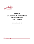
National Semiconductor
Application Note 706
October 1993
Table of Contents
4.4 Initialization
1.0 INTRODUCTION
1.1 Application Note Objectives
1.2 Brief Description of LM628/629
2.0 DEVICE DESCRIPTION
2.1 Hardware Architecture
2.2 Motor Position Decoder
2.3 Trajectory Profile Generator
2.4 Definitions Relating to Profile Generation
2.5 Profile Generation
2.6 Trajectory Resolution
2.7 Position, Velocity and Acceleration Resolution
2.8 Velocity Mode
2.9 Motor Output Port
2.10 Host Interface
2.11 Hardware Busy Bit Operation
2.12 Filter Initial Values and Tuning
3.0 USER COMMAND SET
4.4.1 Hardware RESET Check
4.4.2 Initializing LM628 Output Port
4.4.3 Interrupt Commands
4.5 Performance Refinements
LM628/629 User Guide
LM628/629 User Guide
4.5.1 Derivative Sample Rate
4.5.2 Integral Windup
4.5.3 Profiles other than Trapezoidal
4.5.4 Synchronizing Axes
4.6 Operating Constraints
4.6.1 Updating Acceleration on the Fly
4.6.2 Command Update Rate
5.0 THEORY
5.1 PID Filter
5.1.1 PID Filter in the Continuous Domain
5.1.2 PID Filter Bode Plots
5.2 PID Filter Coefficient Scaling Factors for LM628/629
3.1 Overview
3.2 Host-LM628/629 CommunicationÐthe Busy Bit
3.3 Loading the Trapezoidal Velocity Profile Generator
3.4 Loading PID Filter Coefficients
3.5 Interrupt Control Commands
3.6 Data Reporting Commands
3.7 Software Example
4.0 HELPFUL USER IDEAS
5.2.1 PID Filter Difference Equation
5.2.2 Difference Equation with LM628/629
Coefficients
5.2.3 LM628/629 PID Filter Output
5.2.4 Scaling for kp and kd
5.2.5 Scaling for ki
5.3 An Example of a Trajectory Calculation
6.0 QUESTIONS AND ANSWERS
4.1 Getting Started
4.2 Hardware
4.2.1 Host Microcontroller Interface
4.2.2 Position Encoder Interface
4.2.3 Output Interface
4.3 Software
6.1 The Two Most Popular Questions
6.2 More on Acceleration Change
6.3 More on Stop Commands
6.4 More on Define Home
6.5 More on Velocity
6.6 More on Use of Commands
7.0 ACKNOWLEDGEMENTS
8.0 REFERENCES AND FURTHER READING
AN-706
C1995 National Semiconductor Corporation
TL/H/11018
RRD-B30M75/Printed in U. S. A.
List of Illustrations
Figure 1.
LM628 and LM629 Typical System Block Diagram
Figure 2.
Figure 3.
Figure 4.
Figure 5.
Figure 6.
Figure 7.
Figure 8.
Figure 9.
Figure 10.
Figure 11.
Figure 12.
Figure 13.
Figure 14.
Figure 15.
Figure 16.
Figure 17.
Figure 18.
Figure 19.
Hardware Architecture of LM628/629
Quadrature Encoder Output Signals and Direction Decode Table
LM628/629 Motor Position Decoder
Typical Trajectory Velocity Profile
Position, Velocity and Acceleration Registers
LM628 12-Bit DAC Output Multiplexed Timing
LM629 PWM Output Signal Format
Host Interface Internal I/O Registers
Busy Bit Operation during Command and Data Write Sequence
Position vs Time for 100 Count Step Input
Basic Software Flow
LM628 and LM629 Host, Output and Position Encoder Interfaces
LM628 Example of Linear Motor Drive using LM12
LM629 H-Bridge Motor Drive Example using LM18293
Generating a Non-Trapezoidal Profile
Bode Plots of PID Transfer Function
Scaling for kp and kd
Scaling for ki
Figure 20. Trajectory Calculation Example Profile
Table I.
Trajectory Control Word Bit Allocations
2
Section 5 ‘‘Theory’’ is a short foray into theory which relates
the PID coefficients that would be calculated from a continuous domain control loop analysis to those of the discrete
domain including the scaling factors inherent to the
LM628/629. No attempt is made to discuss control system
theory as such, readers should consult the ample references available, some suggestions are made at the end of
this application note. Section 5 concludes with an example
trajectory calculation, reviving those perhaps forgotten
ideas about acceleration, velocity, distance and time.
Section 6 ‘‘Questions and Answers’’, is in question and answer format and is born out of and dedicated to the many
interesting discussions with customers that have taken
place.
1.0 INTRODUCTION
1.1 Application Note Objective
This application note is intended to explain and complement
the information in the data sheet and also address the common user questions. While no initial familiarity with the
LM628/629 is assumed, it will be useful to have the
LM628/629 data sheet close by to consult for detailed descriptions of the user command set, timing diagrams, bit
assignments, pin assignments, etc.
After the following brief description of the LM628/629, Section 2.0 gives a fairly full description of the device’s operation, probably more than is necessary to get going with the
device. This section ends with an outline of how to tune the
control system by adjusting the PID filter coefficients.
Section 3 ‘‘User Command Set’’ discusses the use of the
LM628/629 commands. For a detailed description of each
command the user should refer to the data sheet.
Section 4 ‘‘Helpful User Ideas’’ starts with a short description of the actions necessary to get going, then proceeds to
talk about some performance enhancements and follows on
with a discussion of a couple of operating constraints of the
device.
1.2 Brief Description of LM628/629
LM628/629 is a microcontroller peripheral that incorporates
in one device all the functions of a sample-data motion control system controller. Using the LM628/629 makes the potentially complex task of designing a fast and precise motion
control system much easier. Additional features, such as
trajectory profile generation, on the ‘‘fly’’ update of loop
compensation and trajectory, and status reporting, are included. Both position and velocity motion control systems
can be implemented with the LM628/629.
TL/H/11018 – 1
FIGURE 1. LM628 and LM629 Typical System Block Diagram
3
to the other input of the summing junction and subtracted
from the demand position to form the error signal input for
the control loop compensator. The compensator is in the
form of a ‘‘three term’’ PID filter (proportional, integral, derivative), this is implemented by a digital filter. The coefficients
for the PID digital filter are most easily determined by tuning
the control system to give the required response from the
load in terms of accuracy, response time and overshoot.
Having characterized a load these coefficient values are
downloaded from the host before commencing a move. For
a load that varies during a movement more coefficients can
be downloaded and used to update the PID filter at the moment the load changes. All trajectory parameters except acceleration can also be updated while a movement is in progress.
LM628/629 is itself a purpose designed microcontroller that
implements a position decoder, a summing junction, a digital
PID loop compensation filter, and a trajectory profile generator, Figure 1. Output format is the only difference between
LM628 and LM629. A parallel port is used to drive an 8- or
12-bit digital-to-analog converter from the LM628 while the
LM629 provides a 7-bit plus sign PWM signal with sign and
magnitude outputs. Interface to the host microcontroller is
via an 8-bit bi-directional data port and six control lines
which includes host interrupt and hardware reset. Maximum
sampling rates of either 2.9 kHz or 3.9 kHz are available by
choosing the LM6268/9 device options that have 6 MHz or
8 MHz maximum clock frequencies (device -6 or -8 suffixes).
In operation, to start a movement, a host microcontroller
downloads acceleration, velocity and target position values
to the LM628/629 trajectory generator. At each sample interval these values are used to calculate new demand or
‘‘set point’’ positions which are fed into the summing junction. Actual position of the motor is determined from the
output signals of an optical incremental encoder. Decoded
by the LM628/629’s position decoder, actual position is fed
2.0 DEVICE DESCRIPTION
2.1 Hardware Architecture
Four major functional blocks make up the LM628/629 in
addition to the host and output interfaces. These are the
Trajectory Profile Generator, Loop Compensating PID Filter,
Summing Junction and Motor Position Decoder (Figure 1) .
TL/H/11018 – 2
FIGURE 2. Hardware Architecture of LM628/629
4
to provide position and direction information, Figure 3 . Optionally a third index position output signal can be used to
capture position once per revolution. Each of the four states
of the quadrature position signal are decoded by the
LM628/629 giving a 4 times increase in position resolution
over the number of encoder lines. An ‘‘N’’ line encoder will
be decoded as ‘‘4N’’ position counts by LM628/629.
Position decoder block diagram, Figure 4, shows three lines
coming from the shaft encoder, M1, M2 and Index. From
these the decoder PLA determines if the motor has moved
forward, backward or stayed still and then drives a 16-bit updown counter that keeps track of actual motor position.
Once per revolution when all three lines including the index
line are simultaneously low, Figure 3, the current position
count is captured in an index latch.
Details of how LM628/629 is implemented by a purpose
designed microcontroller are shown in Figure 2. The control
algorithm is stored in a 1k x 16-bit ROM and uses 16-bit
wide instructions. A PLA decodes these instructions and
provides data transfer timing signals for the single 16-bit
data and instruction bus. User variable filter and trajectory
profile parameters are stored as 32-bit double words in
RAM. To provide sufficient dynamic range a 32-bit position
register is used and for consistency. 32 bits are also used
for velocity and acceleration values. A 32-bit ALU is used to
support the 16 x 16-bit multiplications of the error and PID
digital filter coefficients.
2.2 Motor Position Decoder
LM628/629 provides an interface for an optical position
shaft encoder, decoding the two quadrature output signals
TL/H/11018 – 3
FIGURE 3. Quadrature Encoder Output Signals and Direction Decode Table
TL/H/11018 – 4
FIGURE 4. LM628/629 Motor Position Decoder
5
The 16-bit up-down counter is used to capture the difference in position from one sample to the next. A position
latch attached to the up-down counter is strobed at the
same time in every sample period by a sync pulse that is
generated in hardware. The position latch is read soon after
the sync pulse and is added to the 32-bit position register in
RAM that holds the actual current position. This is the value
that is subtracted in the summing junction every sample interval from the new desired position calculated by the trajectory generator to form the error input to the PID filter.
Maximum encoder state capture rate is determined by the
minimum number of clock cycles it takes to decode each
encoder state, see Figure 3, this minimum number is 8 clock
cycles, capture of the index pulse is also achieved during
these 8 clock cycles. This gives a more than adequate 1
MHz maximum encoder state capture rate with the 8 MHz
fCLK devices (750 kHz for the 6 MHz fCLK devices). For
example, with the 1 MHz capture rate, a motor using a 500
line encoder will be moving at 30,000 rpm.
There is some limited signal conditioning at the decoder
input to remove problems that would occur due to the asynchronous position encoder input being sampled on signal
edges by the synchronous LM628/629. But there is no
noise filtering as such on the encoder lines so it is important
that they are kept clean and away from noise sources.
e 2048/fCLK) respectively. Velocity is therefore calculated
in counts/sample and acceleration in counts/sample/sample.
Definitions of ‘‘target’’, ‘‘desired’’ and ‘‘actual’’ within the
profile generation activity as they apply to velocity, acceleration and position are as follows. Final requested values are
called ‘‘target’’, such as target position. The values computed by the profile generator each sample interval on the way
to the target value are called ‘‘desired’’. Real values from
the position encoder are called ‘‘actual’’.
For example, the current actual position of the motor will
typically be a few counts away from the current desired position because a new value for desired position is calculated
every sample interval during profile generation. The difference between the current desired position and current actual position relies on the ability of the control loop to keep the
motor on track. In the extreme example of a locked rotor
there could be a large difference between the current actual
and desired positions.
Current desired velocity refers to a fixed velocity at any
point on a on-going trajectory profile. While the profile demands acceleration, from zero to the target velocity, the
velocity will incrementally increase at each sample interval.
Current actual velocity is determined by taking the difference in the actual position at the current and the previous
sample intervals. At velocities of many counts per sample
this is reasonably accurate, at low velocities, especially below one count per sample, it is very inaccurate.
2.3 Trajectory Profile Generator
Desired position inputs to the summing junction, Figure 1,
within the LM628/629 are provided by an internal independent trajectory profile generator. The trajectory profile generator takes information from the host and computes for
each sample interval a new current desired position. The
information required from the host is, operating mode, either
position or velocity, target acceleration, target velocity and
target position in position mode.
2.5 Profile Generation
Trajectory profiles are plotted in terms of velocity versus
time, Figure 5, and are velocity profiles by reason that a new
desired position is calculated every sample interval. For
constant velocity these desired position increments will be
the same every sample interval, for acceleration and deceleration the desired position increments will respectively increase and decrease per sample interval. Target position is
the integral of the velocity profile.
2.4 Definitions Relating to Profile Generation
The units of position and time, used by the LM628/629, are
counts (4 c N encoder lines) and samples (sample intervals
TL/H/11018 – 5
FIGURE 5. Typical Trajectory Velocity Profile
6
When performing a move the LM628/629 uses the information as specified by the host and accelerates until the target
velocity is reached. While doing this it takes note of the
number of counts taken to reach the target velocity. This
number of counts is subtracted from the target position to
determine where deceleration should commence to ensure
the motor stops at the target position. LM628/629 deceleration rates are equal to the acceleration rates. In some cases, depending on the relative target values of velocity, acceleration and position, the target velocity will not be
reached and deceleration will commence immediately from
acceleration.
2.7 Position, Velocity and Acceleration Resolution
Every sample cycle, while the profile demands acceleration,
the acceleration register is added to the velocity register
which in turn is added to the position register. When the
demand for increasing acceleration stops, only velocity is
added to the position register. Only integer values are output from the position register to the summing junction and
so fractional position counts must accumulate over many
sample intervals before an integer count is added and the
position register changed. Figure 6 shows the position, velocity and acceleration registers.
The position dynamic range is derived from the 32 bits of
the integer position register, Figure 6. The MSB is used for
the direction sign in the conventional manner, the next bit
30 is used to signify when a position overflow called ‘‘wraparound’’ has occurred. If the wraparound bit is set (or reset
when going in a negative direction) while in operation the
status byte bit 4 is set and optionally can be used to interrupt the host. The remaining 30 bits provide the available
dynamic range of position in either the positive or negative
direction ( g 1,073,741,824 counts).
Velocity has a resolution of 1/216 counts/sample and acceleration has a resolution of 1/216 counts/sample/sample
as mentioned above. The dynamic range is 30 bits in both
cases. The loss of one bit is due to velocity and acceleration
being unsigned and another bit is used to detect wraparound. This leaves 14 bits or 16,383 integral counts and 16
bits for fractional counts.
2.6 Trajectory Resolution
The resolution the motor sees for position is one integral
count. The algorithm used to calculate the trajectory adds
the velocity to the current desired position once per sample
period and produces the next desired position point. In order to allow very low velocities it is necessary to have velocities of fractional counts per sample. The LM628/629 in addition to the 32-bit position range keeps track of 16 bits of
fractional position. The need for fractional velocity counts
can be illustrated by the following example using a 500 line
(2000 count) encoder and an 8 MHz clock LM628/629 giving a 256 ms sample interval. If the smallest resolution is 1
count per sample then the minimum velocity would be 2
revolutions per second or 120 rpm. (1/2000 revs/count c
1/256 ms counts/second). Many applications require velocities and steps in velocity less than this amount. This is provided by the fractional counts of acceleration and velocity.
2.8 Velocity Mode
LM628 supports a velocity mode where the motor is commanded to continue at a specified velocity, until it is told to
TL/H/11018 – 6
FIGURE 6. Position, Velocity and Acceleration Registers
7
stop (LTRJ bits 9 or 10). The average velocity will be as
specified but the instantaneous velocity will vary. Velocities
of fractional counts per sample will exhibit the poorest instantaneous velocity. Velocity mode is a subset of position
mode where the position is continually updated and moved
ahead of the motor without a specified stop position. Care
should be exercised in the case where a rotor becomes
locked while in velocity mode as the profile generator will
continue to advance the position. When the rotor becomes
free high velocities will be attained to catch-up with the current desired position.
2.9 Motor Output Port
LM628 output port is configured to 8 bits after reset. The
8-bit output is updated once per sample interval and held
until it is updated during the next sample interval. This allows use of a DAC without a latch. For 12-bit operation the
PORT12 command should be issued immediately after reset. The output is multiplexed in two 6-bit words using pins
18 through 23. Pin 24 is low for the least significant word
and high for the most significant. The rising edge of the
active low strobe from pin 25 should be used to strobe the
output into an external latch, see Figure 7. The DAC output
is offset binary code, the zero codes are hexÊ 80Ê for 8 bits
and hexÊ 800Ê for 12 bits.
TL/H/11018 – 8
Note: Sign output (pin 18) not shown.
FIGURE 8. LM629 PWM Output Signal Format
2.10 Host Interface
LM628/629 has three internal registers: status, high, and
low bytes, Figure 9, which are used to communicate with the
host microcontroller. These are controlled by the RD, WR,
and PS lines and by use of the busy bit of the status byte.
The status byte is read by bringing RD and PS low, bit 0 is
the busy bit. Commands are written by bringing WR and PS
low. When PS is high, WR brought low writes data into
LM628/629 and similarly, RD is brought low to read data
from LM628/629. Data transfer is a two-byte operation written in most to least significant byte order. The above description assumes that CS is low.
TL/H/11018–7
FIGURE 7. LM628 12-Bit DAC Output Multiplexed Timing
The choice of output resolution is dependant on the user’s
application. There is a fundamental trade-off between sampling rate and DAC output resolution, the LM628 8-bit output
at a 256 ms sampling interval will most often provide as
good results as a slower, e.g. microcontroller, implementation which has a 4 ms typical sampling interval and uses a
12-bit output. The LM628 also gives the choice of a 12-bit
DAC output at a 256 ms sampling interval for high precision
applications.
LM629 PWM sign and magnitude signals are output from
pins 18 and 19 respectively. The sign output is used to control motor direction. The PWM magnitude output has a resolution of 8 bits from maximum negative drive to maximum
positive drive. The magnitude output has an off condition,
with the output at logic low, which is useful for turning a
motor off when using a bridge motor drive circuit. The minimum duty cycle is 1/128 increasing to a maximum of
127/128 in the positive direction and a maximum of
128/128 in the negative direcition, i.e., a continuous output.
There are four PWM periods in one LM629 sample interval.
With an 8 MHz clock this increases the PWM output rate to
15.6 kHz from the LM629 maximum 3.9 kHz sample rate,
see Figure 8 for further timing information.
TL/H/11018 – 9
FIGURE 9. Host Interface Internal I/O Registers
2.11 Hardware Busy Bit Operation
Before and between all command byte and data byte pair
transfers, the busy bit must be read and checked to be at
logic low. If the busy bit is set and commands are issued
they will be ignored and if data is read it will be the current
contents of the I/O buffer and not the expected data. The
busy bit is set after the rising edge of the write signal for
commands and the second rising edge of the respective
read or write signal for two byte data transfers, Figure 10.
The busy bit remains high for approximately 15 ms.
8
TL/H/11018 – 10
FIGURE 10. Busy Bit Operation during Command and Data Write Sequence
sired and actual position and velocity, to see if the error
between desired and actual positions of the motor are constant and not increasing without bound. See Section 3.6 and
the data sheet for information about the reporting commands. Clearly it will be difficult to tune for best system
response if the motor and its load cannot achieve the demanded values of acceleration and velocity. When correct
operation is confirmed and limiting values understood, filter
tuning can commence.
Due to the basic difficulty of accurately modeling a control
system, with the added problem of variations that can occur
in mechanical components over time and temperature, it is
always necessary at some stage to perform tuning empirically. Determining the PID filter coefficients by tuning is the
preferred method with LM628/629 because of the inherent
flexibility in changing the filter coefficients provided by this
programmable device.
Before tuning a control system the effect of each of the PID
filter coefficients should be understood. The following is a
very brief review, for a detailed understanding reference (2)
should be consulted. The proportional coefficient, kp, provides adjustment of the control system loop proportional
gain, as this is increased the output steady state error is
reduced. The error between the required and actual position
is effectively divided by the loop gain. However there is a
natural limitation on how far kp can be increased on its own
to reduce output position error because a reduction in
phase margin is also a consequence of increasing kp. This
is first encountered as ringing about the final position in response to a step change input and then instability in the
form of oscillation as the phase margin becomes zero. To
improve stability, kd, the derivative coefficient, provides a
damping effect by providing a term proportional to velocity
in antiphase to the ringing, or viewed in another way, adds
some leading phase shift into the loop and increases the
phase margin.
In the tuning process the coefficients kp and kd are iteratively increased to their optimum values constrained by the system constants and are trade-offs between response time,
stability and final position error. When kp and kd have been
determined the integral coefficient, ki, can be introduced to
remove steady state errors at the load. The steady state
The busy bit reset to logic low indicates that high and low
byte registers shown in Figure 9 have been either loaded or
read by the LM628/629 internal microcode. To service the
command or data transfer this microcode which performs
the trajectory and filter calculations is interrupted, except in
critical areas, and the on-going calculation is suspended.
The microcode was designed this way to achieve minimum
latency when communicating with the host. However, if this
communication becomes too frequent and on-going calculations are interrupted too often corruption will occur. In a
256 ms sample interval, the filter calculation takes 50 ms,
outputting a sample 10 ms and trajectory calculation 90 ms.
If the LM628 behaves in a manner that is unexpected the
host communication rate should be checked in relation to
these timings.
2.12 Filter Initial Values and Tuning
When connecting up a system for the first time there may be
a possibility that the loop phasing is incorrect. As this may
cause violent oscillation it is advisable to initially use a very
low value of proportional gain, say kp e 1 (with kd, ki and il
all set to zero), which will provide a weak level of drive to the
motor. (The Start command, STT, is sent to LM628/629 to
close the control loop and energize the motor.) If the system
does oscillate with this low value of kp then the motor connections should be reversed.
Having determined that the loop phasing is correct kp can
be increased to a value of about 20 to see that the control
system basically works. This value of kp should hold the
motor shaft reasonably stiffly, returning the motor to the set
position, which will be zero until trajectory values have been
input and a position move performed. If oscillation or unacceptable ringing occurs with a kp value of 20 reduce this
until it stops. Low values of acceleration and velocity can
now be input, of around 100, and a position move commanded to say 1000 counts. All values suggested here are
decimal. For details of loading trajectory and filter parameters see Section 3.0, reference (5) and the data sheet.
It is useful at this stage to try different values of acceleration
and velocity to get a feel for the system limitations. These
can be determined by using the reporting commands of de-
9
errors removed are the velocity lag that occurs with a constant velocity output and the position error due to a constant
static torque. A value of integration limit, il, has to be input
with ki, otherwise ki will have no effect. The integral coefficient ki adds another variable to the system to allow further
optimization, very high values of ki will decrease the phase
margin and hence stability, see Section 5 and reference (2)
for more details. Reference (5) gives more details of PID
filter tuning and how to load filter parameters.
TABLE I. Trajectory Control Word Bit Allocations
Bit Position
Figure 11 illustrates how a relatively slow response with
overshoot can be compensated by adjustment of the PID
filter coefficients to give a faster critically damped response.
3.0 USER COMMAND SET
3.1 Overview
The following types of User Commands are available:
Initialization
Filter control commands
Trajectory control commands
Interrupt control commands
Data reporting commands
User commands are single bytes and have a varying number of accompanying data bytes ranging from zero to fourteen depending upon the command. Both filter and trajectory control commands use a double buffered scheme to input
data. These commands load primary registers with multiple
words of data which are only transferred into secondary
working registers when the host issues a respective single
byte user command. This allows data to be input before its
actual use which can eliminate any potential communication
bottlenecks and allow synchronized operation of multiple
axes.
Function
Bit 15
Bit 14
Bit 13
Bit 12
Not Used
Not Used
Not Used
Forward Direction (Velocity Mode Only)
Bit 11
Bit 10
Bit 9
Bit 8
Velocity Mode
Stop Smoothly (Decelerate as Programmed)
Stop Abruptly (Maximum Deceleration)
Turn Off Motor (Output Zero Drive)
Bit
Bit
Bit
Bit
7
6
5
4
Not Used
Not Used
Acceleration Will Be Loaded
Acceleration Data Is Relative
Bit
Bit
Bit
Bit
3
2
1
0
Velocity Will Be Loaded
Velocity Data Is Relative
Position Will Be Loaded
Position Data Is Relative
Bits 0 to 5 determine whether any, all or none of the position, velocity or acceleration values are loaded and whether
they are absolute values or values relative to those previously loaded. All trajectory values are 32-bit values, position
values are both positive and negative. Velocity and acceleration are 16-bit integers with 16-bit fractions whose absolute
value is always positive. When entering relative values ensure that the absolute value remains positive. The manual
stop commands bits 8, 9 and 10 are intended to allow an
unprogrammed stop in position mode, while a position move
is in progress, perhaps by the demand of some external
event, and to provide a method to stop in velocity mode.
They do not specify how the motor will stop in position
mode at the end of a normal position move. In position
mode a programmed move will automatically stop with a
deceleration rate equal to the acceleration rate at the target
position. Setting a stop bit along with other trajectory parameters at the beginning of a move will result in no movement!
Bits 8, 9 and 10 should only be set one at a time, bit 8 turns
the motor off by outputting zero drive to the motor, bit 9
stops the motor at maximum deceleration by setting the target position equal to the current position and bit 10 stops
the motor using the current user-programmed acceleration
value. Bit 11 is set for operating in velocity mode and bit 12
is set for forward direction in velocity mode.
3.2 Host-LM628/629 CommunicationÐThe Busy Bit
Communication flow between the LM628/629 and its host
is controlled by using a busy bit, bit 0, in the Status Byte.
The busy bit must be checked to be at logic 0 by the host
before commands and data are issued or data is read. This
includes between data byte pairs for commands with multiple words of data.
3.3 Loading the Trapezoidal Velocity Profile Generator
To initiate a motor move, trajectory generator values have
to be input to the LM628/629 using the Load Trajectory
Parameters, LTRJ, command. The command is followed by
a trajectory control word which details the information to be
loaded in subsequent data words. Table I gives the bit allocations, a bit is set to logic 1 to give the function shown.
Underdamped
Critically Damped
TL/H/11018 – 11
FIGURE 11. Position vs Time for 100 Count Step Input
10
the LM628/629 is programmed to interrupt its host, the
event which caused this interrupt can be determined from
bits 1 to 6 of the Status Byte (additionally bit 0 is the busy bit
and bit 7 indicates that the motor is off). All the Interrupt
Control commands are executable during motion.
The Mask Interrupts command, MSKI, is used to tell
LM628/629 which of bits 1 to 6 will interrupt the host
through use of interrupt mask data associated with the command. The data is in the form of a data byte pair, bits 1 – 6 of
the least significant byte being set to logic 1 when an interrupt source is enabled. The Reset Interrupts command,
RSTI, resets interrupt bits in the Status Byte by sending a
data byte pair, the least significant byte having logic 0 in bit
positions 1 to 6 if they are to be reset.
Executing the Set Index Position command, SIP, causes bit
3 of the status byte to be set when the absolute position of
the next index pulse is recorded in the index register. This
can be read with the command, Read Index Position, RDIP.
Executing either Load Position Error for Interrupt, LPEI, or
Load Position Error for Stopping, LPES, commands, sets bit
5 of the Status Byte when a position error exceeding a
specified limit occurs. An excessive position error can indicate a serious system problem and these two commands
give the option when this occurs of either interrupting the
host or stopping the motor and interrupting the host. The
excessive position is specified following each command by
a data byte pair in most to least significant byte order.
Executing either Set Break Point Absolute, SBPA, or Set
Break Point Relative, SBPR, commands, sets bit 6 of the
status byte when either the specified, absolute or relative,
breakpoint respectively is reached. The data for SBPA can
be the full position range (hexÊ C0000000Ê to Ê 3FFFFFFFÊ )
and is sent in two data byte pairs in most to least significant
byte order. The data for the Set Breakpoint Relative command is also of two data byte pairs, but its value should be
such that when added to the target position it remains within
the absolute position range. These commands can be used
to signal the moment to update the on-going trajectory or
filter coefficients. This is achieved by transferring data from
the primary registers, previously loaded using LTRJ or LFIL,
to working registers, using the STT or UDF commands.
Interrupt bits 1, 2 and 4 of the Status Byte are not set by
executing interrupt commands but by events occurring during LM628/629 operation as follows. Bit 1 is the command
error interrupt, bit 2 is the trajectory complete interrupt and
bit 4 is the wraparound interrupt. These bits are also
masked and reset by the MSKI and RSTI commands respectively. The Status Byte still indicates the condition of
interrupt bits 1 – 6 when they are masked from interrupting
the host, allowing them to be incorporated in a polling
scheme.
Following immediately after the trajectory control word
should be two 16-bit data words for each parameter specified to be loaded. These should be in the descending order
of the trajectory control word bits, that is acceleration, velocity and position. They are written to the LM628/629 as
two pairs of data bytes in most to least significant byte order. The busy bit should be checked between the command
byte and the data byte pair forming the trajectory control
word and the individual data byte pairs of the data. The Start
command, STT, transfers the loaded trajectory data into the
working registers of the double buffered scheme to initiate
movement of the motor. This buffering allows any parameter, except acceleration, to be updated while the motor is
moving by loading data with the LTRJ command and to be
later executed by using the STT command.
New values of acceleration can be loaded with LTRJ while
the motor is moving, but cannot be executed by the STT
command until the trajectory has completed or the drive to
the motor is turned off by using bit 8 of the trajectory control
word. If acceleration has been changed and STT is issued
while the drive to the motor is still present, a command error
interrupt will be generated and the command ignored. Separate pairs of LTRJ and STT commands should be issued to
first turn the motor off and then update acceleration. System
operation when changing acceleration while the motor is
moving, but with the drive removed, is discussed in Section
4.5.1.
3.4 Loading PID Filter Coefficients
PID filter coefficients are loaded using the Load Filter Parameters, LFIL, command and are the proportional coefficient kp, derivative coefficient kd and integral coefficient ki.
Associated with ki, an integration limit, il, has to be loaded.
This constrains the magnitude of the integration term of the
PID filter to the il value, see Section 4.4.2. Associated with
the derivative coefficient, a derivative sample rate can be
chosen from 2048/fCLK to (2048 c 256)/fCLK in steps of
2048/fCLK, see Section 4.4.1.
The first pair of data bytes following the LFIL command byte
form the filter control word. The most significant byte sets
the derivative sample rate, the fastest rate, 2048/fCLK, being hexÊ 00Ê the slowest rate (2048 c 256)/fCLK being
hexÊ FFÊ . The lower four bits of the least significant byte tell
the LM628/629 which of the coefficients is going to be loaded, bit 3 is kp, bit 2 is ki, bit 1 is kd and bit 0 is il. Each filter
coefficient and the integration limit can range in value from
hexÊ 0000Ê to Ê 7FFFÊ , positive only. If all coefficient values
are loaded then ten bytes of data, including the filter control
word, will follow the LFIL command. Again the busy bit has
to be checked between the command byte and filter control
word and between data byte pairs. Use of new filter coefficient values by the LM628/629 is initiated by issuing the
single byte Update Filter command, UDF.
When controlled movement of the motor has been
achieved, by programming the filter and trajectory, attention
turns to incorporating the LM628/629 into a system. Interrupt Control Commands and Data Reporting Commands enable the host microcontroller to keep track of LM628/629
activity.
3.6 Data Reporting Commands
Read Status Byte, RDSTAT, supported by a hardware register accessed via CS, RD and PS control, is the most frequently used method of determining LM628/629 status.
This is primarily to read the busy bit 0 while communicating
commands and data as described in Section 3.2.
There are seven other user commands which can read data
from LM628/629 data registers.
3.5 Interrupt Control Commands
There are five commands that can be used to interrupt the
host microcontroller when a predefined condition occurs
and two commands that control interrupt operation. When
11
Read Desired Velocity, RDDV, reads the current desired velocity used to calculate the desired position profile by the
trajectory generator. It is a 32-bit value containing integer
and fractional velocity information. Read Real Velocity,
RDRV, reads the instantaneous actual velocity and is a 16bit integer value.
Read Integration-Term Summation Value, RDSUM, reads
the accumulated value of the integration term. This is a 16bit value ranging from zero to the current, il, integration limit
value.
The Read Signals Register command, RDSIGS, returns a
16-bit data word to the host. The least-significant byte repeats the RDSTAT byte except for bit 0 which indicates that
a SIP command has been executed but that an index pulse
has not occurred. The most significant byte has 6 bits that
indicate set-up conditions (bits 8, 9, 11, 12, 13 and 14). The
other two bits of the RDSIGS data word indicate that the
trajectory generator has completed its function, bit 10, and
that the host interrupt output (Pin 17) has been set to logic
1, bit 15. Full details of the bit assignments of this command
can be found in the data sheet.
The Read Index Position, RDIP, command reads the position recorded in the 32 bits of the index register in four data
bytes. This command, with the SIP command, can be used
to acquire a home position or successive values. These
could be used, for example, for gross error checking.
Both on-going 32-bit position inputs to the summing junction
can be read. Read desired position, RDDP, reads the current desired position the demand or ‘‘set point input’’ from
the trajectory generator and Read Real Position, RDRP,
reads the current actual position of the motor.
LABEL
MNEMONIC
Initialization:
WAIT
RDSTAT
3.7 Software Example
The following example shows the flow of microcontroller
commands needed to get the LM628/629 to control a simple motor move. As it is non-specific to any microcontroller
pseudo commands WR,XXXXH and RD,XXXXH with hex immediate data will be used to indicate read and write operations respectively by the host to and from the LM628/629.
Decisions use IF..THEN..ELSE. BUSY is a user routine to
check the busy bit in the Status Byte, WAIT is a user routine
to wait 1.5 ms after hardware reset.
:REMARK
:Routine to wait 1.5 ms after reset.
:Check correct RESET operation by reading the
:Status Byte. This should be either hexÊ 84Ê or Ê C4Ê
IF Status byte not equal hexÊ 84Ê or Ê C4Ê THEN repeat
hardware RESET
:Make decision concerning validity of RESET
Optionally the Reset can be further checked for correct operation as follows. It is useful to include this to reset all interrupt bits in
the Status Byte before further action:
MSKI
:Mask interrupts
BUSY
:Check busy bit 0 routine
WR,0000H
:Host writes two zero bytes of data to
:LM628/629. This mask disables all interrupts.
BUSY
:Check busy bit
RSTI
:Reset Interrupts command
BUSY
:Check busy bit
WR,0000H
:Host writes two zero bytes of data to LM628/629
RDSTAT
:Status byte should read either hexÊ 80Ê or Ê C0Ê
IF Status byte not equal hexÊ 80Ê or Ê C0Ê THEN repeat
hardware RESET
:
IF Status Byte equal to hexÊ C0Ê THEN continue ELSE PORT
:
BUSY
:Check busy bit
RSTI
:Reset Interrupts
BUSY
:Check busy bit
WR,0000H
:Reset all interrupt bits
Set Output Port Size for a 12-bit DAC.
PORT
BUSY
:Check busy bit
PORT12
:Sets LM628 output port to 12-bits
(Only for systems with 12-bit DAC)
12
Load Filter Parameters
BUSY
LFIL
BUSY
WR,0008H
BUSY
WR,0032H
:Check busy bit
:Load Filter Parameters command
:Check busy bit
:Filter Control Word
:
Bits 8 to 15 (MSB) set the derivative
:sample rate.
:
Bit 3
Loading kp data
:
Bit 2
Loading ki data
:
Bit 1
Loading kd data
:
Bit 0
Loading il data
:Choose to load kp only at maximum
:derivative sample rate then Filter Control
:Word 4 0008H
:Check busy bit
:Choose kp 4 50, load data byte pair MS
:byte first
Update Filter
BUSY
:Check busy bit
UDF
:
Load Trajectory Parameters
BUSY
:Check busy bit
LTRJ
:Load trajectory parameters command.
BUSY
:Check busy bit
WR,002AH
:Load trajectory control word:
:
See Table I
:Choose Position mode, and load absolute
:acceleration, velocity and position. Then
:trajectory control word 4 002AH. This means
:6 pairs of data bytes should follow.
BUSY
:Check busy bit
WR,XXXXH
:Load Acceleration integer word MS byte first
BUSY
:Check busy bit
WR,XXXXH
:Load Acceleration fractional word MS byte first
BUSY
:Check busy bit
WR,XXXXH
:Load Velocity integer word MS byte first
BUSY
:Check busy bit
WR,XXXXH
:Load Velocity fractional word MS byte first
BUSY
:Check busy bit
WR,XXXXH
:Load Position MS byte pair first
BUSY
:Check busy bit
WR,XXXXH
:Load position LS byte pair
Start Motion
BUSY
:Check busy bit
STT
:Start command
Check for Trajectory complete.
RDSTAT
:Check Status Byte bit 2 for trajectory
:complete
Busy bit check routine
BUSY
RDSTAT
:Read status byte
If bit 0 is set THEN BUSY ELSE RETURN
END
*Consult reference (5) for more information on programming the LM628/629.
13
TL/H/11018 – 12
FIGURE 12. Basic Software Flow
14
4.0 HELPFUL USER IDEAS
4.2.2 Position Encoder Interface
4.1 Getting Started
This section outlines the actions that are necessary to implement a simple motion control system using LM628/629.
More details on how LM628/629 works and the use of the
User Command Set are given in the sections ‘‘2.0 DEVICE
DESCRIPTION’’ and ‘‘3.0 USER COMMAND SET’’.
The two optical incremental position encoder outputs feed
into the LM628/629 quadrature decoder TTL inputs A and
B. The leading phase of the quadrature encoder output defines the forward direction of the motor and should be connected to input A. Optionally an index pulse may be used
from the position encoder. This is connected to the IN input,
which should be tied high if not used, see Figure 13.
4.2 Hardware
The following hardware connections need to be made:
4.2.3 Output Interface
LM628 has a parallel output of either 8 or 12 bits, the latter
is output as two multiplexed 6-bit words. Figure 14 illustrates
how a motor might be driven using a LM12 power linear
amplifier from the output of 8-bit DAC0800.
LM629 has a sign and magnitude PWM output, Figure 13, of
7-bit resolution plus sign. Figure 15 shows how the LM629
sign and magnitude outputs can be used to control the outputs of an LM18293 quad half-H driver. The half-H drivers
are used in pairs, by using 100 mX current sharing resistors,
and form a full-H bridge driver of 2A output. The sign bit is
used to steer the PWM LM629 magnitude output to either
side of the H-bridge lower output transistors while holding
the upper transistors on the opposite side of the H-bridge
continuously on.
4.2.1 Host Microcontroller Interface
Interface to the host microcontroller is via an 8-bit command/data port which is controlled by four lines. These are
the conventional chip select CS, read RD, write WR and a
line called Port Select PS, see Figure 13. PS is used to
select user Command or Data transfer between the
LM628/629 and the host. In the special case of the Status
Byte (RDSTAT) bringing PS, CS and RD low together allows
access to this hardware register at any time. An optional
interrupt line, HI, from the LM628/629 to the host can be
used. A microcontroller output line is necessary to control
the LM628/629 hardware reset action.
TL/H/11018 – 13
FIGURE 13. LM628 and LM629 Host, Output and Position Encoder Interfaces
TL/H/11018 – 14
FIGURE 14. LM628 Example of
Linear Motor Drive Using LM12
15
TL/H/11018 – 15
FIGURE 15. LM629 H-Bridge Motor Drive Example Using LM18293
16
interval is loaded with the filter coefficient values as the
most significant byte of the LFIL control word everytime the
command is used, the host therefore needs to store the
current value for re-loading at times of filter coefficient
change.
4.3 Software
Making LM628/629 perform a motion control function requires that the host microcontroller, after initializing
LM628/629, loads coefficients for the PID filter and then
loads trajectory information. The interrupt and data reporting commands can then be used by the host to keep track
of LM628/629 actions. For detailed descriptions see the
LM628/629 data sheet and Section 3.
4.5.2 Integral Windup
Along with the integral filter coefficient, ki, an integration
limit, il, has to be input into LM628/629 which allows the
user to set the maximum value of the integration term of
equation (3), Section 5.2.2. This term is then able to accumulate up to the value of the integration limit and any further
increase due to error of the same sign is ignored. Setting
the integration limit enables the user to prevent an effect
called ‘‘Integral Windup’’. For example, if an LM628/629
attempts to accelerate a motor at a faster rate than it can
achieve, a very large integral term will result. When the
LM628/629 tries to stop the motor at the target position the
large accumulated integral term will dominate the filter and
cause the motor to badly overshoot, and thus integral windup has occurred.
4.4 Initialization
There is only one initialization operation that must be performed; a check that hardware reset has operated correctly.
If required, the size of the LM628 output port should be
configured. Other operations which might be part of user’s
system initialization are discussed under Interrupt and Data
Reporting commands, Sections 3.5 and 3.6.
4.4.1 Hardware RESET Check
The hardware reset is activated by a logic low pulse at pin
27, RST, from the host of greater than 8 clock cycles. To
ensure that this reset has operated correctly the Status Byte
should be checked immediately after the reset pin goes
high, it should read hexÊ 00Ê . If the reset is successful this
will change to hexÊ 84Ê or Ê C4Ê within 1.5 ms. If not, the hardware reset and check should be repeated. A further check
can be used to make certain that a reset has been successful by using the Reset Interrupts command, RSTI. Before
sending the RSTI, issue the Mask Interrupts command,
MSKI, and mask data that disables all interrupts, this mask
is sent as two bytes of data equaling hexÊ 0000Ê . Then issue
the RSTI command plus mask data that resets all interrupts,
this equals hexÊ 0000Ê and is again sent as two bytes. Do not
forget to check the busy bit between the command byte and
data byte pairs. When the chip has reset properly the status
byte will change from hexÊ 84Ê or Ê C4Ê to hexÊ 80Ê or Ê C0Ê .
4.5.3 Profiles Other Than Trapezoidal
TL/H/11018 – 16
FIGURE 16. Generating a Non-Trapezoidal Profile
If it is required to have a velocity profile other than trapezoidal, this can be accomplished by breaking the profile into
small pieces each of which is part of a small trapezoid. A
piecewise linear approximation to the required profile can
then be achieved by changing the maximum velocity before
the trapezoid has had time to complete, see Figure 16.
4.4.2 Initializing LM628 Output Port
Reset sets the LM628 output port size to 8 bits. If a 12-bit
DAC is being used, then the output port size is set by the
use of the PORT12 command.
4.4.3 Interrupt Commands
Optionally the commands which cause the LM628/629 to
take action on a predefined condition (e.g., SIP, LPEI, LPES,
SBPA and SBPR) can be included in the initialization, these
are discussed under Interrupt Commands.
4.5.4 Synchronizing Axes
For controlling tightly coupled coordinated motion between
multiple-axes, synchronization is required. The best possible
synchronization that can be achieved between multiple
LM628/629 is within one sample interval, (2048/fCLK,
256 ms for an 8 MHz clock, 341 ms for a 6 MHz clock). This
is achieved by using the pipeline feature of the LM628/629
where all controlled axes are loaded individually with trajectory values using the LTRJ command and then simultaneously given the start command STT. PID filter coefficients
can be updated in a similar manner using LFIL and UDF
commands.
4.5 Performance Refinements
4.5.1 Derivative Sample Rate
The derivative sample interval is controllable to improve the
stability of low velocity, high inertia loads. At low speeds,
when fractional counts for velocity are used, the integer position counts, desired and actual, only change after several
sample intervals of the LM628/629 (2048/fCLK). This
means that for sample intervals between integer count
changes the error voltage will not change for successive
samples. As the derivative term, kd, multiplies the difference
betweeen the previous and current error values, if the derivative sample interval is the same as the sample interval,
several consecutive sample intervals will have zero derivative term and hence no damping contribution. Lengthening
the derivative sample interval ensures a more constant derivate term and hence improved stability. Derivative sample
4.6 Operating Constraints
4.6.1 Updating Acceleration on the Fly
Whereas velocity and target position can be updated while
the motor is moving, on the ‘‘fly’’, the algorithm described in
Section 2.5 prevents this for acceleration. To change acceleration while the motor is moving in mid-trajectory the motor
off command has to be issued by setting LTRJ command bit
8. Then the new acceleration can be loaded, again using the
17
LTRJ command. When the start command STT is issued
the motor will be energized and the trajectory generator will
start generating a new profile from the actual position when
the STT command was issued. In doing this the trajectory
generator will assume that the motor starts from a stationary
position in the normal way. If the motor has sufficient inertia
and is still moving when the STT command is issued then
the control loop will attempt to bring the motor on to the
new profile, possibly with a large error value being input to
the PID filter and a consequential saturated output until the
motor velocity matches the profile. This is a classic case of
overload in a feedback system. It will operate in an open
loop manner until the error input gets within controllable
bounds and then the feedback loop will close. Performance
in this situation is unpredictable and application specific.
LM628/629 was not intentionally designed to operate in this
way.
4.6.2 Command Update Rate
If an LM628/629 is updated too frequently by the host it will
not keep up with the commands given. The LM628/629
aborts the current trajectory calculation when it receives a
new STT command, resulting in the output staying at the
value of the previous sample. For this reason it is recommended that trajectory is not updated at a greater rate than
once every 10 ms.
5.0 THEORY
5.1 PID Filter
5.1.1 PID Filter in the Continuous Domain
The LM628/629 uses a PID filter as the loop compensator,
the expression for the PID filter in the continuous domain is:
H(s) e Kp a Ki/s a Kds
(1)
Where
Kp e proportional coefficient
Ki e integral coefficient
Kd e derivative coefficient
5.1.2 PID Filter Bode Plots
TL/H/11018 – 17
FIGURE 17. Bode Plots of PID Transfer Function
18
The Bode plots for this function (shown in Figure 17 ) show
the effect of the individual terms of equation (1). The proportional term, Kp provides adjustment of proportional gain.
The derivative term Kd increases the system bandwidth but
more importantly adds leading phase shift to the control
loop at high frequencies. This improves stability by counteracting the lagging phase shift introduced by other control
loop components such as the motor. The integral term, Ki,
provides a high DC gain which reduces static errors, but
introduces a lagging phase shift at low frequencies. The relative magnitudes of Kd, Ki and loop proportional gain have
to be adjusted to achieve optimum performance without introducing instability.
Where:
kp, ki and kd are the discrete-time LM628/629 coefficients
e(n) is the position error at sample time n
nÊ indicates sampling at the derivative sampling rate.
The error signal e(n) [or e(nÊ )] is a 16-bit number from the
output of the summing junction and is the input to the PID
filter. The 15-bit filter coefficients are respectively multiplied
by the 16-bit error terms as shown in equation (3) to produce 32-bit products.
5.2.3 LM628/629 PID Filter Output
The proportional coefficient kp is multiplied by the error signal directly. The error signal is continually summed at the
sample rate to previously accumulated errors to form the
integral signal and is maintained to 24 bits. To achieve a
more usable range from this term, only the most significant
16 bits are used and multiplied by the integral coefficient, ki.
The absolute value of this product is compared with the
integration limit, il, and the smallest value, appropriately
signed, is used. To form the derivative signal, the previous
error is subtracted from the current error over the derivative
sampling interval. This is multiplied by the derivative coefficient kd and the product contributes every sample interval
to the output independently of the user chosen derivative
sample interval.
The least significant 16 bits of the 32-bit products from the
three terms are added together to produce the resulting u(n)
of equation (3) each sample interval. From the PID filter 16bit result, either the most significant 8 or 12 bits are output,
depending on the output word size being used. A consequence of this and the use of the 16 MSB’s of the integral
signal is a scaling of the filter coefficients in relation to the
continuous domain coefficients.
5.2 PID Filter Coefficient Scaling Factors for LM628/629
While the easiest way to determine the PID filter coefficient
kp, kd, and ki values is to use tuning as described in Section
2.11, some users may want to use a more theoretical approach to at least find initial starting values before fine tuning. As very often this analysis is performed in the continuous (s) domain and transformed into the discrete digital domain for implementation, the relationship between the continuous domain coefficients and the values input into
LM628/629 is of interest.
5.2.1 PID Filter Difference Equation
In the discrete domain, equation (1) becomes the difference
equation:
N
u(n) e Kpe(n) a KiT
&e(n)
a Kd/Ts [e(n) b e(n b 1)]
(2)
ne0
Where:
T is the sample interval 2048/fCLK
Ts is the derivative sample interval (2048/fCLK c (1..255)
5.2.2 Difference Equation with LM628/629 Coefficients
In terms of LM628/629 coefficients, (2) becomes:
5.2.4 Scaling for kp and kd
Figure 18 gives details of the multiplication and output for kp
and kd. Taking the output from the MS byte of the LS 16 bits
of the 32-bit result register causes an effective 8-bit rightshift or division of 256 associated with kp and kd as follows:
N
u(n) e kpe(n) a ki
& e(n)
a kd [e(nÊ ) b e(nÊ b 0)]
(3)
ne0
TL/H/11018 – 18
FIGURE 18. Scaling of kp and kd
19
Result e kp c e(n)/256 e Kp x e(n) .Ê . kp
e 256 c Kp.
Problem: Determine the trajectory parameters for a motor
move of 500 revolutions in 1 minute with 15 seconds of
acceleration and deceleration respectively. Assume the optical incremental encoder used has 500 lines.
Similarly for kd:
Result e (kd x [e(nÊ ) b e(nÊ b1)])/256
e Kd/Ts c e(n) .Ê . kd e 256 c Kd/Ts
Where Ts is the derivative sampling rate.
The LM628/629 quadrature decoder gives four counts for
each encoder line giving 2000 counts per revolution in this
example. The total number of counts for this position move
is 2000 c 500 e 1,000,000 counts.
By definition, average velocity during the acceleration and
deceleration periods, from and to zero, is half the maximum
velocity. In this example, half the total time to make the
move (30 seconds) is taken by acceleration and deceleration. Thus in terms of time, half the move is made at maximum velocity and half the move at an average velocity of
half this maximum. Therefore, the combined distance traveled during acceleration and deceleration is half that during
5.2.5 Scaling for ki
Figure 19 shows the multiplication and output for the integral term ki. The use of a 24-bit register for the error terms
summation gives further scaling:
Result e ki/256 c l e(n)/256
e Ki c T .Ê . ki e 65536 Ki c T.
Where T is the sampling interval 2048/fCLK.
For a 12-bit output the factors are:
kp e 16 c Kp, kd e 16 c Kd/Ts and ki e 4096 Ki c T.
If the 32-bit result register overflows into the most significant
16-bits as a result of a calculation, then all the lower bits are
set high to give a predictable saturated output.
5.3 An Example of a Trajectory Calculation
TL/H/11018 – 19
FIGURE 19. Scaling for ki
TL/H/11018 – 20
FIGURE 20. Trajectory Calculation Example Profile
20
maximum velocity or (/3 of the total, or 333,333 counts. Acceleration and deceleration takes 166,667 counts respectively.
6.2.2 Is there any way to change acceleration?
Answer: Acceleration change can be simulated by making
many small changes of maximum velocity. For instance if a
small velocity change is loaded, using LTRJ and STT commands, issuing these repeatedly at predetermined time intervals will cause the maximum velocity to increment producing a piecewise linear acceleration profile. The actual
acceleration between velocity increments remains the
same.
The time interval used by the LM628/629 is the sample
interval which is 256 ms for a fCLK of 8 MHz.
The number of sample periods in 15 seconds e 15s/
256 ms e 58,600 samples
Remembering that distance s e at2/2 is traveled due to
acceleration Ê aÊ and time Ê tÊ .
Therefore acceleration a e 2S/t2
e 2 c 166,667/58,600
e 97.1 c 10 b 6 counts/sample2
Acceleration and velocity values are entered into
LM628/629 as a 32-bit integer double-word but represents
a 16-bit integer plus 16-bit fractional value. To achieve this
acceleration and velocity decimal values are scaled by
65536 and any remaining fractions discarded. This value is
then converted to hex to enter into LM628 in four bytes.
Scaled acceleration a e 97.1 c 10b6 c 65536
6.3 More on Stop Commands
6.3.1 What happens if the on-going trajectory is
stopped by setting LTRJ control word bits 9 or 10, stop
abruptly or stop smoothly, and then restarted by issuing Start, STT?
Answer: While stopped the motor position will be held by
the control loop at the position determined as a result of
issuing the stop command. Issuing STT will cause the motor
to restart the trajectory toward the original target position
with normal controlled acceleration.
6.3.2 What happens if the on-going trajectory is
stopped by setting LTRJ control word bit 8, motor-off?
Answer: The LM628’s DAC output is set to mid-scale, this
puts zero volts on the motor which will still have a dynamic
braking effect due to the commutation diodes. The LM629’s
PWM output sets the magnitude output to zero with a similar
effect. If the motor freewheels or is moved the desired and
actual positions will be the same. This can be verified using
the RDDP and RDRP commands. When Start, STT, is issued the loop will be closed again and the motor will move
toward the original trajectory from the actual current position.
6.3.3 If the motor is off, how can the control loop be
closed and the motor energized?
Answer: Simply by issuing the Start, STT command. If any
previous trajectory has completed then the motor will be
held in the current position. If a trajectory was in progress
when the motor-off command was issued then the motor
will restart and move to the target position in position mode,
or resume movement in velocity mode.
e 6.36 decimal e 00000006 hex.
The maximum velocity can be calculated in two ways, either
by the distance in counts traveled at maximum velocity divided by the number of samples or by the acceleration multiplied by the number of samples over acceleration duration,
as follows:
Velocity e 666,667/117,200 e 97.1 c 10b6 c 58,600
e 5.69 counts/sample
Scaled by 65536 becomes 372,899.8 decimal e 0005B0A3
hex.
Inputting these values for acceleration and velocity with the
target position of 1,000,000 decimal, 000F4240 hex will
achieve the desired velocity profile.
6.0 QUESTIONS AND ANSWERS
6.1 The Two Most Popular Questions
6.1.1 Why doesn’t the motor move, I’ve loaded filter parameters, trajectory parameters and issued Update Filter, UDF, and Start, STT, commands?
Answer: The most like cause is that a stop bit (one of bits 8,
9 or 10 of the trajectory control word) has been set in error,
supposedly to cause a stop in position mode. This is unnecessary, in position mode the trajectory stops automatically
at the target position, see Section 3.3.
6.4 More on Define Home
6.4.1 What happens if the Define Home command, DFH,
is issued while a current trajectory is in progress?
Answer: The position where the DFH command is issued is
reset to zero, but the motor still stops at the original position
commanded, i.e., the position where DFH is issued is substracted from the original target position.
6.4.2 Does issuing Define Home, DFH, zero both the trajectory and position register.
Answer: Yes, use Read Real Position, RDRP, and Read Desired Position, RDDP to verify.
6.1.2 Can acceleration be changed on the fly?
Answer: No, not directly and a command error interrupt will
be generated when STT is issued if acceleration has been
changed. Acceleration can be changed if the motor is
turned off first using bit 8 of the Load Trajectory Parameter,
LTRJ, trajectory control word, see Section 4.6.1.
6.2.More on Acceleration Change
6.2.1 What happens at restart if acceleration is changed
with the motor drive off and the motor is still moving?
Answer: The trajectory generation starting position is the
actual position when the STT command is issued, but assumes that the motor is stationary. If the motor is moving
the control loop will attempt to bring the motor back onto an
accelerating profile, producing a large error value and less
than predictable results. The LM628/629 was not designed
with the intention to allow acceleration changes with moving
motors.
6.5 More on Velocity
6.5.1 Why is a command error interrupt generated when
inputting negative values of relative velocity?
Answer: Because the negative relative velocity would cause
a negative absolute velocity which is not allowed. Negative
absolute values of velocity imply movement in the negative
direction which can be achieved by inputting a negative po-
21
sition value or in velocity mode by not setting bit 12. Similarly negative values of acceleration imply deceleration which
occurs automatically at the acceleration rate when the
LM628/629 stops the motor in position mode or if making a
transition from a higher to a lower value of velocity.
6.5.2 What happens in velocity (or position) mode when
the position range is exceeded?
Answer: The position range extends from maximum negative position hexÊ C0000000Ê to maximum positive position
hexÊ 3FFFFFFFÊ using a 32-bit double word. Bit 31 is the
direction bit, logic 0 indicates forward direction, bit 30 is the
wraparound bit used to control position over-range in velocity (or position) mode.
When the position increases past hexÊ 3FFFFFFFÊ the wraparound bit 30 is set, which also sets the wraparound bit in
the Status byte bit 4. This can be polled by the host or
optionally used to interrupt the host as defined by the MSKI
commands. Essentially the host has to manage wraparound
by noting its occurrence and resetting the Status byte wraparound bit using the RSTI command. When the wraparound
bit 30 is set in the position register so is the direction bit.
This means one count past maximum positive position
hexÊ 3FFFFFFFÊ moves the position register onto the maximum negative position hexÊ C0000000Ê . Continued increase
in positive direction causes the position register to count up
to zero and back to positive values of position and on
toward another wraparound.
Similarly when traveling in a negative direction, using two’s
complement arithmetic, position counts range from
hexÊ FFFFFFFÊ (b1 decimal) to the maximum negative position of hexÊ C0000000Ê . One more negative count causes
the position register to change to hexÊ 3FFFFFFFÊ , the maximum positive position. This time the wraparound bit 30 is
reset, causing the wraparound bit 4 of the status byte to be
set. Also the direction bit 31 is reset to zero. Further counts
in the negative direction cause the position register to count
down to zero as would be expected. With management
there is no reason why absolute position should be lost,
even when changing between velocity and position modes.
6.6.5 What happens if the motor is not able to keep up
with the specified trajectory acceleration and velocity
values?
Answer: A large, saturated, position error will be generated,
and the control loop will be non-linear. The acceleration and
velocity values should be set within the capability of the
motor. Read Desired and Real Position commands, RDDP
and RDRP can be used to determine the size of the error.
The Load Position Error commands, for either host Interrupt
or motor Stopping, LPEI and LPES, can be used to monitor
the error size for controlled action where safety is a factor.
6.6.6 When is the command error bit 1 in the Status
Byte set?
Answer:
a) When an acceleration change is attempted when the motor is moving and the drive on.
b) When loading a relative velocity would cause a negative
absolute velocity.
c) Incorrect reading and writing operations generally.
6.6.7 What does the trajectory complete bit 2 in the
Status Byte indicate?
Answer: That the trajectory loaded by LTRJ and initiated by
STT has completed. The motor may or may not be at this
position. Bit 2 is also set when the motor stop commands
are executed and completed.
6.6.8 What do the specified minimum and maximum values of velocity mean in reality?
Answer: Assume a 500 line encoder e 1/2000 revs/count
is used.
The maximum LM628/629 velocity is 16383 counts/sample
and for a 8 MHz clock the LM628/629 sample rate is 3.9k
samples/second, multiplying these values gives 32k revs/
second or 1.92M rpm.
The maximum encoder rate is 1M counts/second multiplied
by 1/2000 revs/count gives 500 revs/second or 30k rpm.
The encoder capture rate therefore sets the maximum velocity limit.
The minimum LM628/629 velocity is 1/65536 counts/sample (one fractional count), multiplying this value by the sample rate and encoder revs/count gives 30 c 10b6 revs/
second or 1.8 c 10b3 rpm.
The LM628 provides no limitation to practical values of velocity.
6.6.9 How long will it take to get to position wraparound
in velocity mode traveling at 5000 rpm with a 500 line
encoder?
Answer: 107 minutes.
6.6 More on Use of Commands
6.6.1 If filter parameter and trajectory commands are
pipelined for synchronization of axes, can the Update
Filter, UDF, and Start, STT, commands be issued consecutively?
Answer: Yes.
6.6.2 Can commands be issued between another command and its data?
Answer: No.
6.6.3 What is the response time of the set breakpoint
commands, SBPA and SBPR?
Answer: There is an uncertainty of one sample interval in
the setting of the breakpoint bit 6 in the Status Byte in response to these commands.
6.6.4 What happens when the Set Index Position, SIP,
command is issued?
Answer: On the next occurrence of all three inputs from the
position encoder being low the corresponding position is
loaded into the index register. This can be read with the
Read Index Position command, RDIP. Bit 0 of the Read Signals register, shows when an SIP command has been issued but the index position has not yet been acquired.
RDSIGS command accesses the Read Signals Register.
7.0 REFERENCES AND FURTHER READING
1. LM628/LM629 Precision Motion Controller. Data sheet
March 1989.
2. Automatic Control Systems. Benjamin C. Kuo. Fifth edition Prentice-Hall 1987.
3. DC Motors, Speed Controls, Servo Systems. Robbins &
Myers/Electro Craft.
4. PID Algorithms and their Computer Implementation. D.W.
Clarke. Institute of Measurement and Control, Trans. v. 6
No. 6 Oct/Dec 1984 86/178.
5. LM628 Programming Guide. Steven Hunt. National Semiconductor Application Note AN-693.
22
23
LM628/629 User Guide
LIFE SUPPORT POLICY
NATIONAL’S PRODUCTS ARE NOT AUTHORIZED FOR USE AS CRITICAL COMPONENTS IN LIFE SUPPORT
DEVICES OR SYSTEMS WITHOUT THE EXPRESS WRITTEN APPROVAL OF THE PRESIDENT OF NATIONAL
SEMICONDUCTOR CORPORATION. As used herein:
AN-706
1. Life support devices or systems are devices or
systems which, (a) are intended for surgical implant
into the body, or (b) support or sustain life, and whose
failure to perform, when properly used in accordance
with instructions for use provided in the labeling, can
be reasonably expected to result in a significant injury
to the user.
National Semiconductor
Corporation
2900 Semiconductor Drive
P.O. Box 58090
Santa Clara, CA 95052-8090
Tel: 1(800) 272-9959
TWX: (910) 339-9240
National Semiconductor
GmbH
Livry-Gargan-Str. 10
D-82256 F4urstenfeldbruck
Germany
Tel: (81-41) 35-0
Telex: 527649
Fax: (81-41) 35-1
National Semiconductor
Japan Ltd.
Sumitomo Chemical
Engineering Center
Bldg. 7F
1-7-1, Nakase, Mihama-Ku
Chiba-City,
Ciba Prefecture 261
Tel: (043) 299-2300
Fax: (043) 299-2500
2. A critical component is any component of a life
support device or system whose failure to perform can
be reasonably expected to cause the failure of the life
support device or system, or to affect its safety or
effectiveness.
National Semiconductor
Hong Kong Ltd.
13th Floor, Straight Block,
Ocean Centre, 5 Canton Rd.
Tsimshatsui, Kowloon
Hong Kong
Tel: (852) 2737-1600
Fax: (852) 2736-9960
National Semiconductores
Do Brazil Ltda.
Rue Deputado Lacorda Franco
120-3A
Sao Paulo-SP
Brazil 05418-000
Tel: (55-11) 212-5066
Telex: 391-1131931 NSBR BR
Fax: (55-11) 212-1181
National Semiconductor
(Australia) Pty, Ltd.
Building 16
Business Park Drive
Monash Business Park
Nottinghill, Melbourne
Victoria 3168 Australia
Tel: (3) 558-9999
Fax: (3) 558-9998
National does not assume any responsibility for use of any circuitry described, no circuit patent licenses are implied and National reserves the right at any time without notice to change said circuitry and specifications.