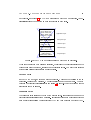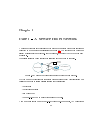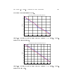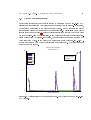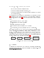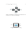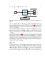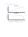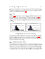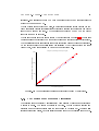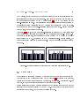
1
Helsinki University of Technology Faculty of Electronics, Communications and Automation Juha Järvinen Testing and Troubleshooting with Passive Network Measurements Master's thesis submitted in partial fulllment of the requirements for the degree of Master of Science in Technology Espoo, 27th January 2009 Supervisor: Professor Raimo Kantola Instructor: Lic.Sc.(Tech.) Marko Luoma HELSINKI UNIVERSITY OF TECHNOLOGY ABSTRACT OF MASTER'S THESIS Author: Juha Järvinen Title: Date: Testing and Troubleshooting with Passive Network Measurements Faculty: Faculty of Electronics, Communications and Automation Department: Department of Communications and Networking Supervisor: Professor Raimo Kantola Instructor: Lic.Sc.(Tech.) Marko Luoma 27th January 2009 Language: English Number of pages: xiii + 95 Code: S-38 This thesis is divided into two parts. In the theory part, the state-of-the-art of passive measurement methods and mechanisms are presented with particular regard to testing and troubleshooting. Secondly, a real world network and network device are measured. The rst measurements concentrate on the troubleshooting in a network of the service hotel. The second case's tests cover the network properties of a single network device. It is found that the fundamental measuring techniques of passive monitoring have remained unchanged, only the link speeds and technologies have renewed it. With modern home computing comes the possibility of doing end-to-end measurements easily. There are new amended methods to measure things easier, more reliably, and requiring smaller amounts of captured data. Troubleshooting the networks does not need to be done just by searching reasons for problems randomly. In the network troubleshooting the suitable model depends on a case. In Case I "A Service Hotel Network" the exclusion model was used partly for searching reasons for problems. The largest problem still remains in time-related multipoint measurements: the availability of cost eective accurate clock synchronization methods for PCs. In addition, capturing data fully from the link speed of 1 Gbit/s and more, is still a problem. Passive packet monitoring is a powerful yet sometimes quite slow way for troubleshooting and testing network devices. Keywords: Trac measurements, passive network measurements, packet capture i TEKNILLINEN KORKEAKOULU DIPLOMITYÖN TIIVISTELMÄ Tekijä: Juha Järvinen Työn nimi: Päivämäärä: Testing and Troubleshooting with Passive Network Measurements Tiedekunta: Elektroniikan, tietoliikenteen ja automaation tiedekunta Laitos: Tietoliikenne- ja tietoverkkotekniikan laitos Valvoja: Professori Raimo Kantola Ohjaaja: TkL Marko Luoma 27.1.2009 Kieli: Englanti Sivumäärä: xiii + 95 Koodi: S-38 Tämä diplomityö jakautuu kahteen osaan: kirjallisuuskatsaukseen ja empiiriseen osioon. Kirjallisuuskatsauksessa käsitellään passiivisissa mittauksissa testaamiseen ja ongelmanratkaisuun nykyään käytettäviä tekniikoita ja metodeita. Empiirisessä osiossa mitataan kahta reaalimaailman verkkoa ja verkkokomponenttia. Ensimmäisessä esimerkissä selvitetään palveluhotellin tietoliikenneverkon ongelmia ja toisessa testataan yksittäisen tietoliikennelaitteen verkko-ominaisuuksia. Passiivisten mittausten mittaustekniikka on pohjimmiltaan pysynyt samana, ainoastaan uudet linkkiteknologiat ja -nopeudet ovat uudistaneet sitä. Nykyaikaisilla kotitietokoneilla voidaan hoitaa joitakin päästä päähän -tyyppisiä mittauksia vaivattomasti. Mittauksiin ja tulosten analysointiin liittyvien metodien kehittymisen, uudistamisen ja lisääntymisen myötä asioita voidaan nykyään mitata helpommin, luotettavammin ja vähemmän mittaustiedon varassa. Tietoverkko-ongelmien syiden etsimiseen tarkoitettujen mallien sopivuus riippuu tapauksesta, esimerkiksi poissulkevaa mallia käytettiin pääasiassa palveluhotelliesimerkissä. Suurimpana ongelmana teollisuus-PC:itä käytettäessä passiivisiin mittauksiin on yhä edelleen tarpeeksi tarkan ajan saaminen. Lisäksi 1 Gbit/s ja sitä suurempien linjanopeuksien täysi talteenottaminen on yhä ongelmallista. Passiivinen pakettimittaus on tehokas, mutta välillä melko hidas tapa verkko-ongelmien selvittämiseksi ja verkkolaitteiden testaamiseksi. Avainsanat: Liikennemittaukset, passiiviset tietoverkkomittaukset, pakettikaappaus ii Preface This work has been done at the Department of Communications and Networking in Helsinki University of Technology, Finland. I would like to thank my supervisor, professor Raimo Kantola and my instructor Lic.Sc.(Tech.) Marko Luoma for their contribution to this master's thesis. Also, Lic.Sc.(Tech.) Markus Peuhkuri and D.Sc.(Tech.) Mika Ilvesmäki deserve my gratitude for providing me with many useful hints and advices on the work. I would also like to thank my colleagues at Department of Communications and Networking and the former Networking Laboratory for friendly atmosphere. Especially my co-workers Timo-Pekka Heikkinen, Eero Solarmo, Oskari Simola and Anni Matinlauri deserve thanks for supportive discussions and spare time. Finally, I would like to express my gratitude to my family who have helped and supported me throughout my life, kiitos! Last but not least, I would thank my girlfriend käraste Karin for all love. Espoo, 27th January 2009 Juha Järvinen iii Table of Contents Abstract i Lyhennelmä ii Preface iii Table of Contents iv List of Figures viii List of Tables xi Abbreviations xii 1 Introduction 1 1.1 Background . . . . . . . . . . . . . . . . . . . . . . . . . . . . . . . . . . . . 1 1.2 Objective . . . . . . . . . . . . . . . . . . . . . . . . . . . . . . . . . . . . . 2 1.3 Structure of the Thesis . . . . . . . . . . . . . . . . . . . . . . . . . . . . . . 2 2 Network Monitoring Techniques 3 2.1 Why Network Monitoring? . . . . . . . . . . . . . . . . . . . . . . . . . . . . 3 2.2 Methods to Monitor a Network . . . . . . . . . . . . . . . . . . . . . . . . . 5 2.2.1 Passive Monitoring . . . . . . . . . . . . . . . . . . . . . . . . . . . . 6 2.2.2 Active Monitoring . . . . . . . . . . . . . . . . . . . . . . . . . . . . 8 iv 2.2.3 2.3 2.4 Hybrid Monitoring . . . . . . . . . . . . . . . . . . . . . . . . . . . . 9 Connection to Network . . . . . . . . . . . . . . . . . . . . . . . . . . . . . . 11 2.3.1 Link Taps . . . . . . . . . . . . . . . . . . . . . . . . . . . . . . . . . 11 2.3.2 Port Mirroring . . . . . . . . . . . . . . . . . . . . . . . . . . . . . . 12 Reducing the Amount of captured Network Trac . . . . . . . . . . . . . . 13 2.4.1 Filtering . . . . . . . . . . . . . . . . . . . . . . . . . . . . . . . . . . 13 2.4.2 Aggregation . . . . . . . . . . . . . . . . . . . . . . . . . . . . . . . . 15 2.4.3 Sampling . . . . . . . . . . . . . . . . . . . . . . . . . . . . . . . . . 15 2.4.4 Rate Adaptive and Rate Constrained Sampling . . . . . . . . . . . . 17 2.4.5 Challenges in Sampling and Analyzing Sampled Network Data . . . 19 2.4.6 Summary . . . . . . . . . . . . . . . . . . . . . . . . . . . . . . . . . 19 2.5 How Much Trac should be Monitored . . . . . . . . . . . . . . . . . . . . . 20 2.6 Summary . . . . . . . . . . . . . . . . . . . . . . . . . . . . . . . . . . . . . 21 3 Network Monitoring Methods 3.1 3.2 3.3 22 Trac . . . . . . . . . . . . . . . . . . . . . . . . . . . . . . . . . . . . . . . 22 3.1.1 IP Trac The 5-layer TCP/IP Model . . . . . . . . . . . . . . . . 22 3.1.2 MPLS . . . . . . . . . . . . . . . . . . . . . . . . . . . . . . . . . . . 26 3.1.3 Virtual Private Networks . . . . . . . . . . . . . . . . . . . . . . . . 27 3.1.4 Header vs. Packet information . . . . . . . . . . . . . . . . . . . . . 28 Where to Monitor the Trac . . . . . . . . . . . . . . . . . . . . . . . . . . 29 3.2.1 Monitoring at Single Point and at Multiple Points . . . . . . . . . . 29 3.2.2 Measuring at Core versus on the End user side . . . . . . . . . . . . 31 3.2.3 NETI@home . . . . . . . . . . . . . . . . . . . . . . . . . . . . . . . 32 3.2.4 Multicast trac . . . . . . . . . . . . . . . . . . . . . . . . . . . . . . 33 Metrics for Network Measurements . . . . . . . . . . . . . . . . . . . . . . . 34 3.3.1 Throughput . . . . . . . . . . . . . . . . . . . . . . . . . . . . . . . . 34 3.3.2 Round-Trip Time . . . . . . . . . . . . . . . . . . . . . . . . . . . . . 35 v 3.4 3.3.3 One-Way Delay . . . . . . . . . . . . . . . . . . . . . . . . . . . . . . 37 3.3.4 Packet Loss . . . . . . . . . . . . . . . . . . . . . . . . . . . . . . . . 39 3.3.5 Multicast . . . . . . . . . . . . . . . . . . . . . . . . . . . . . . . . . 40 3.3.6 Summary . . . . . . . . . . . . . . . . . . . . . . . . . . . . . . . . . 40 Summary . . . . . . . . . . . . . . . . . . . . . . . . . . . . . . . . . . . . . 41 4 Passive Measurements for Troubleshooting and Testing 42 4.1 Models for Troubleshooting . . . . . . . . . . . . . . . . . . . . . . . . . . . 43 4.2 Which Level or Part in Focus . . . . . . . . . . . . . . . . . . . . . . . . . . 45 4.2.1 Network Services . . . . . . . . . . . . . . . . . . . . . . . . . . . . . 46 4.2.2 Backbone Network . . . . . . . . . . . . . . . . . . . . . . . . . . . . 46 4.2.3 Backbone Network Services . . . . . . . . . . . . . . . . . . . . . . . 46 4.2.4 Network Services of Services . . . . . . . . . . . . . . . . . . . . . . . 47 4.2.5 Snapshot of Current State of Services . . . . . . . . . . . . . . . . . 47 4.2.6 General View of Network . . . . . . . . . . . . . . . . . . . . . . . . 47 4.3 The Network Topology . . . . . . . . . . . . . . . . . . . . . . . . . . . . . . 48 4.4 Intrusion Detection System . . . . . . . . . . . . . . . . . . . . . . . . . . . 49 4.5 Network Tomography . . . . . . . . . . . . . . . . . . . . . . . . . . . . . . . 51 4.6 SLA with Passive Monitoring . . . . . . . . . . . . . . . . . . . . . . . . . . 53 4.7 Summary . . . . . . . . . . . . . . . . . . . . . . . . . . . . . . . . . . . . . 54 5 Case I A Service Hotel Network 55 5.1 Measurement Hardware . . . . . . . . . . . . . . . . . . . . . . . . . . . . . 56 5.2 Packet Flows in the Network . . . . . . . . . . . . . . . . . . . . . . . . . . 57 5.3 Delay . . . . . . . . . . . . . . . . . . . . . . . . . . . . . . . . . . . . . . . 60 5.4 Packet Fragmentation . . . . . . . . . . . . . . . . . . . . . . . . . . . . . . 64 5.5 Network Equipment . . . . . . . . . . . . . . . . . . . . . . . . . . . . . . . 65 5.6 Netvis The Network State Portal . . . . . . . . . . . . . . . . . . . . . . . 65 5.7 Summary . . . . . . . . . . . . . . . . . . . . . . . . . . . . . . . . . . . . . 66 vi 5.7.1 Diculties . . . . . . . . . . . . . . . . . . . . . . . . . . . . . . . . . 70 5.7.2 Models in Use . . . . . . . . . . . . . . . . . . . . . . . . . . . . . . . 70 6 Case II An IP Encrypter 72 6.1 Measurement Hardware . . . . . . . . . . . . . . . . . . . . . . . . . . . . . 74 6.2 Tests for One Component . . . . . . . . . . . . . . . . . . . . . . . . . . . . 74 6.3 6.2.1 Test Setup . . . . . . . . . . . . . . . . . . . . . . . . . . . . . . . . . 74 6.2.2 Throughput . . . . . . . . . . . . . . . . . . . . . . . . . . . . . . . . 74 6.2.3 Delay . . . . . . . . . . . . . . . . . . . . . . . . . . . . . . . . . . . 75 6.2.4 Routing Characteristics . . . . . . . . . . . . . . . . . . . . . . . . . 77 Measurements for Two Components With an Encrypted Tunnel . . . . . . . 79 6.3.1 Throughput . . . . . . . . . . . . . . . . . . . . . . . . . . . . . . . . 79 6.3.2 Delay . . . . . . . . . . . . . . . . . . . . . . . . . . . . . . . . . . . 81 6.3.3 Distribution of Packet Length . . . . . . . . . . . . . . . . . . . . . . 81 6.3.4 The Creation Speed of Security Associations . . . . . . . . . . . . . . 82 6.4 Encryption . . . . . . . . . . . . . . . . . . . . . . . . . . . . . . . . . . . . 83 6.5 Summary . . . . . . . . . . . . . . . . . . . . . . . . . . . . . . . . . . . . . 84 7 Conclusions 85 7.1 Summary . . . . . . . . . . . . . . . . . . . . . . . . . . . . . . . . . . . . . 85 7.2 Future Work . . . . . . . . . . . . . . . . . . . . . . . . . . . . . . . . . . . 86 References 88 vii List of Figures 2.1 A ow chart of passive network monitoring. . . . . . . . . . . . . . . . . . . 5 2.2 A real life hybrid monitoring system. . . . . . . . . . . . . . . . . . . . . . . 10 2.3 Capturing trac by using a link tap in beroptic links. . . . . . . . . . . . . 11 2.4 The gure shows how many monitoring points are needed to cover certain trac volume with two dierent algorithms [CFL+ 05] . . . . . . . . . . . . 21 3.1 The TCP/IP model [Tan02] shown with common protocols. . . . . . . . . . 23 3.2 The IP datagram (version 4) header structure [Pos81b]. . . . . . . . . . . . 24 3.3 The TCP header structure [Pos81c]. . . . . . . . . . . . . . . . . . . . . . . 25 3.4 The UDP header structure [Pos80]. . . . . . . . . . . . . . . . . . . . . . . . 25 3.5 The MPLS header structure [RTF+ 01]. . . . . . . . . . . . . . . . . . . . . . 27 3.6 MPLS layer is located in between the OSI layers 2 and 3. . . . . . . . . . . 27 3.7 Complexity of measurements [Ilv07]. . . . . . . . . . . . . . . . . . . . . . . 31 3.8 The basic idea to measure multicast trac passively. CP means a capturing point and RP means a rendevouz point. . . . . . . . . . . . . . . . . . . . . 33 3.9 A ow of some P2P applications. . . . . . . . . . . . . . . . . . . . . . . . . 35 3.10 Measuring RTT with TCP connection opening packets (SYN). . . . . . . . . 37 4.1 A model of network component parts for testing and troubleshooting. . . . . 45 4.2 An example network, which includes a customer, a core, and a server network. 46 5.1 A gure about connecting a service hotel to a core network. . . . . . . . . . 55 5.2 A general view of the service hotel network. Circles mean network splitters. viii 57 5.3 A view of how to capture trac of a DUT . . . . . . . . . . . . . . . . . . . 58 5.4 Routes used for incoming trac into the hotel. Routes are based on the data presented in Table 5.1. . . . . . . . . . . . . . . . . . . . . . . . . . . . 59 5.5 Routes used for outgoing trac into the hotel. Routes are based on the data presented in Table 5.1. . . . . . . . . . . . . . . . . . . . . . . . . . . . . . . 59 5.6 Correcting the clockskew. . . . . . . . . . . . . . . . . . . . . . . . . . . . . 62 5.7 The oset between the system clock and a stratum 3 NTP server. The measurement time is 3600 seconds. . . . . . . . . . . . . . . . . . . . . . . . 63 5.8 The oset between the system clock and a stratum 3 NTP server. The measurement time is 8 days. . . . . . . . . . . . . . . . . . . . . . . . . . . . 63 5.9 A distribution of the packet lengths (66 - 1514 bytes) of a known end-to-end FTP transfer. . . . . . . . . . . . . . . . . . . . . . . . . . . . . . . . . . . . 64 5.10 A ow chart of the Netvis portal. . . . . . . . . . . . . . . . . . . . . . . . . 66 5.11 A screenshot of the Netvis portal. . . . . . . . . . . . . . . . . . . . . . . . . 67 5.12 Realized measurement cycle during troubleshooting of the service hotel. . . 69 6.1 A gure illustrates how IP encrypters can be used for joining branch oces (BO) to a head oce (HO) safely over the public Internet. . . . . . . . . . . 73 6.2 Functional principle of IP encrypter. . . . . . . . . . . . . . . . . . . . . . . 73 6.3 A test setup for one component testing. G# means a trac generator and/or sink. . . . . . . . . . . . . . . . . . . . . . . . . . . . . . . . . . . . . . . . . 75 6.4 Throughput of unicast trac for one component. . . . . . . . . . . . . . . . 76 6.5 Histogram of the throughput delay in the DUT. . . . . . . . . . . . . . . . . 77 6.6 The Processing speed of OSPF AS External messages as a function of throughput of trac (Average of 0.1 s). . . . . . . . . . . . . . . . . . . . . . 78 6.7 The Processing speed of BGP Update messages as a function of throughput of trac (Average of 1.0 s). . . . . . . . . . . . . . . . . . . . . . . . . . . . 79 6.8 A test setup for testing two network components connected with an encrypted tunnel. . . . . . . . . . . . . . . . . . . . . . . . . . . . . . . . . . . 80 6.9 Throughput for two components with an encrypted tunnel. . . . . . . . . . 80 ix 6.10 Histogram of the delay of the whole system. . . . . . . . . . . . . . . . . . . 81 6.11 A gure presents changes in packet length caused by encryption. . . . . . . 82 6.12 Figures describe the creation speed of security associations (SAs). . . . . . . 83 x List of Tables 2.1 Motivation to network measurements [CM97]. . . . . . . . . . . . . . . . . . 4 2.2 Some reliability calculations for an individual device using Equation 2.1. . . 12 2.3 Summary of dierent sampling methods. [ZMD+ 05] . . . . . . . . . . . . . . 20 3.1 Comparison of capturing data at core or on the customer side. . . . . . . . . 32 5.1 The amount of packets measured at dierent capturing points when the trac enters and leaves the hotel. . . . . . . . . . . . . . . . . . . . . . . . . 60 5.2 The packet delay in milliseconds (ms) between a source point and a destination point when the direction of the trac is into the hotel. . . . . . . . . 61 5.3 The packet delay in milliseconds (ms) between a source point and a destination point when the direction of the trac is out of the hotel. . . . . . . . 61 5.4 Findings of this case. . . . . . . . . . . . . . . . . . . . . . . . . . . . . . . . 68 xi Abbreviations ACK Acknowledge ACL Access Control List AFT Address Forwarding Table AS Autonomous System CPU Central Processing Unit CDMA Code Division Multiple Access CWND Congestion Window DUT Device Under Test DNS Domain Name Service DoS Denial of Service EM Expected Maximization FTP File Transfer Protocol GbE Gigabit Ethernet GPS Global Positioning System HIDS Host-based Intrusion Detection System HTTP Hypertext Transfer Protocol IANA Internet Assigned Numbers Authority IAT Inter-Arrival Time ICMP Internet Control Message Protocol IDS Intrusion Detection Systems IP Internet Protocol IPFIX Internet Protocol Flow Information Export ISAKMP Internet Security Association and Key Management Protocol ISP Internet Service Provider xii LAN Local Area Network LSDB Link-State Database LSP Label Switched Path MCMC Markov Chain Monte Carlo MLE Maximum Likelihood Estimate MIB Management Information Base MPLS Multiprotocol Label Switching MSS Maximum Segment Size NIC Network Interface Card NIDS Network-based Intrusion Detection System NTP Network Time Protocol NUT Network Under Test OD Origin Destination OSI Open Systems Interconnection OWAMP One-Way Active Measurement Protocol OWD One-Way Delay P2P Peer to Peer PLR Packet Loss Ratio QoS Quality of Service RTCP Real-Time Control Protocol RTP Real-Time Transport Protocol RTT Round-Trip Time RPF Reverse Path Forwarding SA Security Association SSH Secure Shell SLA Service Level Agreement SNMP Simple Network Management Protocol TCP Transmission Control Protocol TWAMP Two-Way Active Measurement Protocol UDP User Datagram Protocol VLAN Virtual Local Area Network VPN Virtual Private Network WWW World Wide Web xiii Chapter 1 Introduction 1.1 Background All the time networks are becoming more and more complex. There are no longer just a single protocol networks but multilayer ones. The speed of the links is ever growing, which sets special requirements for dierent parts of network equipment for example, for protocols, performance, and the encryption. Additionally everything needs to work eciently, securely and cost-eectively. This means no leakings between dierent VPNs and VLANs no packet's drop of any kind is allowed up until particular link becomes congested. One major question facing operators everywhere is how to be sure that everything goes ne as well as how black holes can be detected in their networks? Passive network monitoring is very suitable for this purpose. It can be used for searching problems of a single network device, a major problem aecting the whole LAN or core network. Passive network monitoring, however, is not just for problem solving it can also be used for creating network statistics or for measuring network performance. As will be seen in this thesis, it is a very powerful tool in everyday network life. Recently operators have noticed that passive monitoring is no longer the last and the oddest option to put into a network1 . Nowadays, depending on the operator, it is a regular tool in networks. They use it for problem solving, monitoring, and now even for billing, thanks to more and more popular packet data in mobile operator's world. Listening in networks has always been an issue since the very rst telephone lines were erected. The rst "monitors" were, usually unintentionally, telephonists (in Finnish, sent1 According to a guest speaker in a lecture. 1 CHAPTER 1. INTRODUCTION 2 raalisantra ). Later on, governments also became interested in wiretapping, and nowadays perhaps, the most famous wiretapping system is the ECHELON system running in the National Security Agency (NSA) of the USA and its allies. Close to Finland's own borders, the neighboring country Sweden, plans to listen to all communication networks as a part of the country's ght against the criminality [FR08]. 1.2 Objective There are two objectives of this thesis. The rst one is to present the state of the art of passive network measurements related to the troubleshooting of networks. The second objective is to present two dierent passive measurement cases related to testing and troubleshooting in the real world. In these two test cases the decision was to use normal industry PC hardware with suitable network interface cards (NICs) for capturing data. 1.3 Structure of the Thesis The thesis is organized as follows: Chapter 2 covers various network monitoring techniques in principle and in practice. Respectively dierent network monitoring methods are handled in Chapter 3. Chapter 4 combines these previous chapters and adds troubleshooting and testing issues. The two cases are handled in Chapters 5 and 6. Finally Chapter 7 presents the conclusions of this thesis and some future research topics. Chapter 2 Network Monitoring Techniques 2.1 Why Network Monitoring? The purpose of network monitoring is to observe and quantify what is happening in the network. With dierent sizes of magnifying glasses (methods, techniques and tools) we can observe both the microcosmic and macrocosmic events in time or in state. By gathering data actively or passively from the network, we have a great opportunity towards the following actions [Hal03, Peu02]: • Performance tuning: identifying and reducing bottlenecks, balancing resource use, etc. • Troubleshooting: identifying, diagnosing and repairing faults. • Planning: predicting the scale and required resources. • Development and design of new technologies: Understanding of current situation in a network, nding trends and directing the development of new technologies. • Characterization of the trac for providing data for modeling and simulation. • Understanding and controlling complexity: understanding and interaction between components of the network and to conrm that functioning, innovation and new technologies perform as predicted and required. • Identication and correction of pathological behavior. 3 CHAPTER 2. NETWORK MONITORING TECHNIQUES 4 For a closer look we can divide the previous list into three parts. Table 2.1 presents these parties: Internet Service Providers (ISPs), users and vendors. The table shows aspects why these three dierent parts are interested in monitoring the networks. It also presents how these participants measure their interests [CM97]. Table 2.1: Motivation to network measurements [CM97]. Goal ISPs Measure • capacity planning • bandwidth utilization • operations • packets per second • value-added services (e.g. cus- • round trip time (RTT) tomer reports) • RTT variance • usage-based billing • packet loss • reachability • circuit performance Users • monitor performance • routing diagnosis • bandwidth availability • plan upgrades • response time • negotiate service contracts • packet loss • optimize content delivery • reachability • usage policing • connection rates • service qualities Vendors • improve design/conguration of equipment • log analysis • implement real-time debugging/diagnosis h/w • host performance • trace samples of deployed CHAPTER 2. NETWORK MONITORING TECHNIQUES 5 ISPs are interested in transferring maximum amount of data at minimum costs. In addition, the billing should work properly if the commercial ISP is in question. On the contrary, a user can have a totally dierent view: he/she usually wants small delay and very low packet loss in end-to-end connections. A user also wants to have persistent connections with full bandwidth as in an agreement between an ISP and a user. Vendors can be said to be between a user and an ISP. For ISPs they try to produce more ecient and cost eective solutions to forward trac in the network. For users they develop monitoring and measuring software and hardware in order to help a user monitor his/her connections and services. 2.2 Methods to Monitor a Network In a passive monitoring system, we can see three main parts: monitoring point, data collection, and analysis point. In more details, the passive monitoring system can be split in ve parts: packet capturing, preprocessing, statistics exporting, statistics collecting, and postprocessing. A common capturing-analysing chain is presented in Figure 2.1. In the gure the red color means the monitoring phase, the blue color denotes the data collection phase, and the green color describes the analysis phase. Capturing Preprocessing Processing Transfering to Storage Storing Storing Transfering for Analysing Analysis Figure 2.1: A ow chart of passive network monitoring. If there is only one computer in a network measuring the network, these three dierent parts can be located in the same computer. When there are two or more monitoring points, however, they cannot naturally any more be located in the same place. In such cases the data collection point and analysis point can be located in the same place. Generally, we can say that a monitoring point needs a good network card and a good Central Processing Unit (CPU) to capture all the packets. In addition it needs a fast hard disc, whose storage volume, however, does not need to be great. A data collection point needs a lot of hard disc space for storing captured traces. Now hard disc can be slow. And CHAPTER 2. NETWORK MONITORING TECHNIQUES 6 nally, an analysis point needs power for analysis tools and hard disc space for storing results. 2.2.1 Passive Monitoring The purpose of passive monitoring is only to listen to the trac in the network, no packets are sent to the network. It does not, therefore, increase the trac on the network for the measurements. It also measures real trac. There are three dierent ways to gather data from the network [ILP07]: • Data copying in network node • Passive listening • Pass-through measurement device. In the rst choice some networking devices (like some Open Systems Interconnection Reference Model (OSI) layer 2 switches) are congured to forward (or to mirror) all packets, which are seen in a port, to another port where packets are gathered. There can be some performance (congestion and accuracy) issues occurring if high-speed links are combined and forwarded to one port. In passive listening, data on copper or optical links can be copied using splitters (see Figure 2.3). In cases of optical links, it redirects some part of the light signal to another optical bre. The splitter is a passive element and therefore, measurements have no eect on normal operation. This is due to the fact when using the splitters trac cannot be injected onto a link. In addition, in cases of power supply problems, splitters are usually capable of transmitting the trac in spite of this. In optical splitters there is no need for any power supply. Using a pass-through measurement device is perhaps the worst option. The link is connected to the measurement device and it copies all the incoming data to the outgoing link verbatim. If there are some problems in the functioning of the device or, for example, problems with current supply, the network trac will be disturbed. In addition, there are a lot of normal network devices (routers, switches) which keep the book from the trac in links on some level. Usually in this kind of devices, a Remote Network Monitoring Management Information Base (RMON MIB) is implemented and used at least. With Simple Network Management Protocol (SNMP), there is no possibility CHAPTER 2. NETWORK MONITORING TECHNIQUES 7 to get information about an individual packet seen on a link, but it is rather for getting a general picture of the network state. For example, you can get from RMON MIB the following information: • Sent and received trac in bit/s on a link • Routing tables • Dierent types of errors occurred on a link • Amount of packets sent/received itemized of transport layer protocols. SNMP is used for fetching statistics from the network devices to one computer where this data can be post-processed. For example, by polling with time intervals of 5 minutes it is possible to display the utilization rate of links connected to a router. Some vendors have the same kind of systems the best known is Cisco's NetFlow which is meant mainly for Cisco's routers and switches. It is based on observing ows in links not packets as in SNMP. The huge amount of captured data, however, is a problem. For example, we have two links with data rates of 1 Gbit/s which we are monitoring. The monitoring point only stores the IP and transport headers (40 bytes per packet) and it can be assumed that the average packet size is 300 bytes. In that case a disk has to store 30 MB/s. If the monitoring point has one 1 TB disk, it can only hold about 9 hours of data. By compressing the amount of stored data this gure can be increased. Dierent ways of compressing captured network data have been explained in [MBG01] and [Peu02]. When collecting data from many high-speed links, there are some performance issues in monitoring devices. Local hard discs in monitoring points can only store the data for a few minutes. In addition, the network has to be quick. This captured data can be decreased either 1) with the pre-processing of data at monitoring points or 2) with the use of sampling when capturing the data from the network. Basically, setting up a passive monitoring system is relatively easy, it being only necessary to connect a monitoring device to the network in some way and then beginning to collect data, and nally analysing data. This is in contrast to the active monitoring of data, where all the tests have to be planned very carefully before execution (see Section 2.2.2). In reality, setting up the passive monitoring system may not be so easy, however. There are two things to think about carefully before execution in order to prevent drowning in the CHAPTER 2. NETWORK MONITORING TECHNIQUES 8 data in analysis phase. First, we have to consider on which level we would like to capture the data: L1 L7. Secondly, we must consider how many bytes of the packet we would like to capture for example is the rst 46 bytes enough or is the whole packet needed. Since passive approach may require viewing all packets on the network, there can be both privacy and/or security issues about how to access and process the data gathered. Security and privacy can be maintained in the following three ways: • Only packet headers should be stored in trace les. However, by picking up only headers, the protocol information is lost. For example, this information is needed for the analysis of routing errors. • Packets should be anonymized in some way as explained in [Peu02] and [Peu01] • Monitoring and monitored devices, and networks should be secured in such a way that unauthorized persons are not able to access the captured data. 2.2.2 Active Monitoring Active monitoring relies on the capability to inject test packets into the network or send packets to servers and applications, to follow them and to measure the service obtained from the network. As such it articially creates extra trac into the network. The volume and other parameters of the introduced trac are fully adjustable. Small trac volumes are usually enough to obtain meaningful measurements. Unfortunately, creating extra trac increases the network load and may cause congestion. Active monitoring provides explicit control on the generation of packets for measurement scenarios. This means control of the nature of trac generation, the sampling techniques, the timing, frequency, scheduling, packet sizes and types, statistical quality, the path, and function chosen to be monitored. [Cot01] There are a lot of dierent active measurement systems on the market. Some are meant for application Quality of Service (QoS) monitoring (e.g WWW-server monitoring) and some are intended for monitoring of networks. They can use either normal computers or dedicated hardware. The round-trip time (RTT) between the source and the destination can be measured very easily, for example, ping command uses ICMP Echo packets (Internet Control Message Protocol [Pos81a]) to infer this information. It is possible to inject ping type probes from any accessible host, making active monitoring well suited to end-to-end performance measurements. CHAPTER 2. NETWORK MONITORING TECHNIQUES 9 In general, active monitoring is used to study the underlying network whereas passive monitoring is most often used for examining the trac in it. The majority of ISPs use active monitoring systems to check the operation of their systems and services. In addition, the fulllment of QoS requirements, stated in the customer's Service Level Agreement (SLA), can be checked by using active monitoring systems. [Vii04, Hei08] From the monitoring equipment, active measurements do not require a great deal. In the simplest case we can test networks with a few ICMP packets. It is good to remember that one protocol can only test one part of network performance and, therefore, a lot of individual tests have to be generated to test the whole network performance. Although there are lot of individual tests in active monitoring systems, tests can rarely cover all the services in the network the most important services from the customer's point of view, for example IP packet switching and Domain Name System (DNS) service, have to be selected rst. Naturally, the most important services to be tested depend on the dierent needs of dierent participants as presented in Table 2.1. There is one important question when active monitoring is used: does this kind of monitoring present realistic result of the network state? If probing with ICMP packets, are results consistent for the rest of services? Does the Internet Service Provider (ISP) give better performance for the probes, for example, for ICMP probes than for normal trac? More reliable results can be achieved by using dierent protocols for probing. This issue is discussed in greater detail in Heikkinen's Master's thesis [Hei08]. There is also another problem with active monitoring. This problem concerns also the passive monitoring under certain situations. If probes are sent periodically every N th second, it might not be possible to notice all the faults in the network or in the services. Probing can be done more frequently but it generates even more extra trac into the network. The amount of individual tests and targets have to be considered very carefully when planning continuous measurements. [Wil03] In active monitoring, security and privacy issues are not a major problem as they are with passive monitoring systems. At monitoring point, the content of normal trac is not studied. In addition to this, connections created by a user are not observed. 2.2.3 Hybrid Monitoring By combining the best features of active and passive monitoring, more realistic and better results can be obtained than by using only one. The solution is hybrid monitoring. This CHAPTER 2. NETWORK MONITORING TECHNIQUES 10 is an interesting study area, but unfortunately a real hybrid monitoring device does not exist, but only in theory. While we can simultaneously gain more information about the properties of the networks, there are, however, properties which can only be measured with one or the other of the monitoring methods. Hybrid method is discussed in an article written by Zangrilli et al. [ZL03]. Using a combination of active and passive monitoring it is possible to get accurate, timely available bandwidth measurements by using passive measurements only when an application is running and active measurements only when none are running. This is done at the same time while limiting the invasiveness of active probes. In the article, mentioned above, a prototype of the Wren bandwidth monitoring tool was built. Practically, this kind of a monitoring system is thought to be like a hybrid monitoring it has an active and a passive part, and an analysing system which combines results from both parts as illustrated in Figure 2.2. There are some measurement devices, which include active measurement functionalities as well as passive monitoring ports, on the market like EtherNID by Accedian1 . But in reality it is not a hybrid monitoring device, since it does not combine these two methods. Figure 2.2: A real life hybrid monitoring system. 1 www.accedian.com CHAPTER 2. NETWORK MONITORING TECHNIQUES 11 2.3 Connection to Network To be able to analyse the status of the network, a connection to network must exist in someway. In active monitoring devices there has to be either L3 addresses (like IP addresses) for communicating with other devices globally, and/or L2 addresses (like MAC addresses) for local communicating. In passive monitoring, however, the situation is dierent: devices only listen to trac in links requiring no IP address. There are three practical ways of connecting passive monitoring device to analysed network: using link taps, port mirroring in switch, or by using hubs. The last one is, however, no longer relevant option in faster networks than 10 Mbps Ethernet. The listening of the trac is not allowed to create or cause any disturbance to the ongoing real trac. In port mirroring and link taps, sending trac to the monitored network is usually not possible. 2.3.1 Link Taps A link tap is used to copy trac from a link to another destination. There are two type of taps: beroptic and copper. A part of trac heading from source A to B is split to the capturing port Bmon , where a monitor listens to trac. This is illustrated in Figure 2.3. Since beroptic taps are passive (in other words there is no delivery of current to the taps) the light power has to split in some ratio. This ratio can be from 90:10 to 50:50 depending on technique used and the length of the link. Copper taps need the delivery of current for copying trac to capturing ports. Figure 2.3: Capturing trac by using a link tap in beroptic links. All kind of devices in the network have an eect on the system reliability. For example, CHAPTER 2. NETWORK MONITORING TECHNIQUES 12 both optical and electrical devices, such as link taps, have reliability, which is always smaller than 1. The overall system reliability is a product of the reliability of individual devices as shown in Equation 2.1. Table 2.2 presents some reliability calculations for an individual device using this equation. The reliability for the whole system is rsys when n devices are in the chain. All the individual devices in the chain have the same reliability. n Y (2.1) ri = rsys i=1 Table 2.2: Some reliability calculations for an individual device using Equation 2.1. ri rsys n=2 n=5 n=10 n=20 0.948683298 0.979148362 0.989519258 0.994745826 0.9 0.994987437 0.997991952 0.998995471 0.999497609 0.99 0.999499875 0.99979992 0.999899955 0.999949976 0.999 0.999949999 0.999979999 0.99999 0.999995 0.9999 From Equation 2.1 and Table 2.2 we see that the more devices the chain has the better reliability one device needs to have in order to achieve a certain reliability rsys . Additionally, if a new device is added to the chain, the reliability of the old devices has to increase in order to maintain the same level of system reliability rsys . It is also found that to achieve the system reliability rsys , the reliability of an individual device has to be approximately ten fold better. Adding a device with lower reliability (ri =0.9) into the chain of 10 devices with better reliability (ri =0.9999) shows how much a new device can lower the reliability of the whole chain. In this case, the original system reliability was 0.999 and after adding the extra device it was no more than rsys =0.8991. 2.3.2 Port Mirroring Port mirroring is a quick, cheap and simple method to copy trac for a monitoring device. Nowadays many switches support port mirroring on some level. This does not, however, guarantee the quality of the mirroring, which partially depends on the switch fabric (SF) architecture used in the switch. Traditionally, four dierent SF designs are used: Shared CHAPTER 2. NETWORK MONITORING TECHNIQUES 13 Memory, Shared Medium, Crossbar and Output buered SFs with N 2 Disjoint Paths. With low trac volume there are no great dierences between designs, but high data rates reveal these dierences clearly. The design aects whether the switch is blocking or non-blocking. In addition, the cheapest switches on the market lack performance, oering very few mirroring options making ecient and reliable mirroring almost impossible. The greatest advantage of it is that it is possible to mirror with some aggregate rule, for example, packets with a certain Virtual Local Area Network (VLAN) tag can be mirrored or trac can be combined from dierent sources and then mirrored. 2.4 Reducing the Amount of captured Network Trac As mentioned earlier, passive monitoring generates a huge amount of data. There are, however, some ways to reduce the amount of data which is stored. These techniques for reducing the amount of data treated and stored can be classied into three main classes [ZMD+ 05, ILP07]: • Filtering Only a subset of the frames on some networking criteria, for example protocol, destination IP address etc., are collected. • Aggregation Packets can be classied into classes and statistics are afterwards calculated by class. • Sampling Packets are collected according to a certain rule. It is good to keep in mind that it is necessary to capture all the packets and bring all of them at least onto some level, which can be a network interface card (NIC), a kernel, or even le system. Where the operations are performed, depends on intelligence of a level. The cheapest way usually is to do it at le system level and the most expensive way is to produce it at NIC level. In a next section we go through these three previous issues in a greater detail. 2.4.1 Filtering Filtering is a deterministic way to select packets. Selection can be based on the packet content, the treatment of the packet at the monitoring point or the deterministic function of these. The packet is selected if one or more of these conditions is fullled. A distinguishing CHAPTER 2. NETWORK MONITORING TECHNIQUES 14 characteristic of ltering is that the selection decision does not depend on the packet position in time or in space, or on a random process. The purpose of ltering is simply to separate the packets into those having a certain property and those not having this certain property. [ZMD+ 05] In addition, there is the possibility to look for particular packet ows in more detail or to completely ignore other packet ows by ltering. On downside, there is not the possibility to gain statement of the entire network usage. In [ZMD+ 05] three dierent ltering techniques are dened: • Field Match Filtering is a stateless ltering mechanism based on IPFIX ow2 denition. A packet is selected if a specic eld in the packet equals a predened value [QBCM05]. • Router State Filtering is a stateful ltering mechanism. Selection is based on one or multiple of the following conditions [ZMD+ 05]: Ingress or egress interface is of a specic value Packet violated Access Control List (ACL) on the router Failed Reverse Path Forwarding (RPF) Resource Reservation is insucient for the packet No route found for the packet 2 Internet Protocol Flow Information Export (IPFIX) is an IETF working group. It was created from the need for a common, universal standard of export for Internet Protocol ow information from routers, probes, trac measurement probes, middleboxes, and other devices that is used by mediation systems, accounting/billing systems, and network management systems to facilitate services such as measurement, accounting, and billing. The IPFIX standard denes how IP ow information is to be formatted and transferred from an exporter to a collector. [QZCZ04] A ow is dened as a set of IP packets passing an observation point in the network during a certain time interval. All packets belonging to a particular ow have a set of common properties. Each property is dened as the result of applying a function to the values of ( [QZCZ04]): one or more packet header eld (e.g., destination IP address), transport header eld (e.g., destination port number), or application header eld one or more characteristics of the packet itself (e.g., number of MPLS labels, etc.) one or more of elds derived from packet treatment (e.g., next hop IP address, the output interface, etc.) A packet is dened to belong to a ow if it completely satises all the dened properties of the ow. CHAPTER 2. NETWORK MONITORING TECHNIQUES 15 Origin/destination Autonomous System (AS) equals a specic value or lies within a given range • Hash-based Filtering. Hash function h maps the packet content c or some portion of it onto a range R. The packet is selected if h(c) is an element of S which is a subset of R called the selection range. Hash-based ltering could be used as random sampling emulation or as consistent packet selection and its application. [ZMD+ 05] 2.4.2 Aggregation The principle of aggregation is to combine with a certain rule packets into one ow. For example, aggregation can be used with network prexes (150.132.54.0/24) or with arbitrary patterns (ports 25 and 80). Aggregation is very useful if we have, for example, Denial Of Service (DOS) attacks when each packet creates a new ow. Resources (memory, CPU etc.) in a monitoring point therefore can be exhausted. In these cases the amount of statistical data is reduced and post-processing is speeded. One disadvantage is that there is loss of detail in statistical information. [FK03] Aggregation can be either made at the monitoring point or at a dedicated aggregator. Resources can be saved if aggregating is done at the monitoring point, not at the collector point. At that time resources can be spent more for the further analysis in the collector point. Unfortunately, aggregation rules have to be implemented at the monitoring point. On the other hand, aggregating in dedicated aggregator resources at the monitoring point can be saved. In addition, simpler monitoring points can be deployed and it is possible to aggregate one or multiple sources. [ILP07] 2.4.3 Sampling Sampling is targeted at the selection of a representative subset of packets. The subset is used to infer knowledge about the whole set of observed packets without processing them all. The selection can depend on packet position, and/or on packet content, and/or on (pseudo) random decisions. The next section considers dierent sampling methods that have been proposed. The following sampling processes are dened by Amer et al. [AC] and Clay et al. [CPB]. CHAPTER 2. NETWORK MONITORING TECHNIQUES 16 Systematic Sampling Systematic sampling is a process of selecting the starting points and the duration of the selection intervals according to a deterministic function, for example, the periodic selection of every N th element of a trace. There is a problem, however, with systematic sampling: if the systematics in the sampling process resembles the systematics in the observed stochastic process, there is high probability that the estimation will be biased [ZMD+ 05]. The only advantage that it has over the random sampling is simplicity. There are two dierent systematic sampling methods: • Systematic count-based (1 in N sampling) • Systematic time-based Systematic Count-based In systematic count-based sampling the start and stop triggers for the sampling interval are dened in relation to the spatial packet position (packet count). Systematic Time-based In systematic time-based sampling time-based start and stop triggers are used to dene the sampling intervals. All packets are selected that arrive at the observation point within the time-intervals dened by the start and stop triggers (i.e. arrival time of the packet is larger than the start time and smaller than the stop time). Random Sampling Random Sampling selects the starting points of the sampling intervals according to a random process [EM97]. The selection of elements are independent experiments. With this, unbiased estimations can be achieved. In contrast to systematic sampling, random sampling requires the generation of random numbers. Random sampling can be classied in the following way [ZMD+ 05]: • Random n-out-of-N sampling selects randomly n elements from a parent population that consists of N elements. CHAPTER 2. NETWORK MONITORING TECHNIQUES 17 • Random Uniform probabilistic sampling selects packets independently with some uniform probability 1/N. If the study is count-driven, it can be referred to as geometric random sampling, since the dierence in counting between successive selected packets are independent random variables with a geometric distribution of mean 1/p. A time-driven analog, exponential random sampling, has the time between triggers exponentially distributed. • Probabilistic sampling samples selection based on a pre-dened selection probability, which eect is like ipping a coin for each packet. • Random Non-uniform ow-state sampling selects packets, probabilistically or deterministically, depending on a selection state. This state depends on the ow state and/or other ow states. An example of such an algorithm is the "sample and hold" method explained in [EV01]: If a packet accounts for a ow record that already exists in the IPFIX ow recording process, it is selected and the ow record is updated If a packet fails to account to any existing ow record, it is selected with probability p. If it has been selected, a new ow record has to be created. Stratied Sampling In the stratied sampling technique, the whole population is rst put into mutually exclusive subgroups or strata and then units are selected randomly from each stratum. The segments are based on some predetermined criteria such as geographic location, size or demographic characteristic. It is important that the segments are as heterogeneous as possible. [EM97] In stratied sampling data is oversampled and then weighted to re-establish the proportions. This technique is often used when one or more of the strata in the population have a low incidence relative to the other stratums. [EM97] 2.4.4 Rate Adaptive and Rate Constrained Sampling Adaptive sampling designs are those in which the selection procedure may depend sequentially on observed values of the variable of interest [Tho87]. Sampling trades o the estimation accuracy against reduction of sampling volumes. The choice of sampling parameters reects the relative need to measure and show trac observed. In practice, there CHAPTER 2. NETWORK MONITORING TECHNIQUES 18 are both systematic and statistical variability in trac streams: Internet trac rates have daily and weekly cycles and link failures lead to rate shifts in trac rates in dierent links. Typically, decisions such as how to sample during an experiment are made and xed in advance. In this section two dierent approaches are presented and discussed for maintaining sampling goals within acceptable limits under variable trac rate conditions. Rate Adaptive Sampling Rate adaptive sampling involves adjusting the sampling rate in response to the rate at which packets are selected or in anticipation of a predicted trac rate. In the paper by Drobisz et al. [DC98] a multiplicative adaptive scheme has been developed to manage resource usage for packet measurement in routers. This paper introduces two dierent controls, one based on CPU utilization and the other based on packet interarrival times. Another paper by Choi et al. [CPZ02] concentrates on maintaining accuracy of estimates of the short-term trac load at a router under varying trac rates. It was noticed that the accuracy of rate estimates determines the resolution at which changes can be detected. The other main issue in this paper was to to identify change-points in the trac load. A totally dierent approach to this issue was described by Hernandez et al. [HCG01] where a predictive approach was used to anticipate variations in the oered load. With this the sampling interval was adjusted accordingly to meet the sampling volume constraints. Rate Constrained Sampling The rate adaptive sampling method has several disadvantages [Duf04]: • Due to the inherent latency of adaption, hard sampling volume constraints cannot be met under arbitrary statistical and systematic variation. • Systematic undersampling is necessary to accommodate uncontrolled variations in the trac rate. • The eective sampling probability is reduced for objects that occur during periods of high load. However, it may be precisely the objects that occur during these periods that are, in fact, the most important to capture. CHAPTER 2. NETWORK MONITORING TECHNIQUES 19 These limitations aect how sampling strategies are able to select a specied number of objects during a given measurement interval [Duf04]. To achieve this, several algorithms have been introduced. In reservoir sampling one keeps a reservoir of k ongoing samples [Vit85]. For non-uniform probability sampling, an algorithm for weighted reservoir with replacement is shown in [CMN99]. 2.4.5 Challenges in Sampling and Analyzing Sampled Network Data If sampling were trouble-free, it would be always used. There are, however, several statistical challenges when sampling and analyzing network measurements [Duf04]: • The majority of available data has already been sampled during collection. Raw unsampled data is increasingly dicult to come by, so it is good to think what the sampled data reveals about the original network trac. • Implementions of sample designs may be limited by technology and resources. Technological constraints may limit the ability to use the sample design that is ideal from a purely statistical point of view. In addition, measurements somehow travel from the monitoring point to the eventual data repository, possibly with some preprocessing or aggregation on the way. Each stage in the journey oers an opportunity for sampling. At which stage sampling is best performed, that is another question. • The best choice of sample design depends on trac characteristics. Experimental studies show that the network trac exhibits dependence and rate uctuations over multiple time scales, leading to heavy-tailed distributions for some trac statistics. Sample design needs to take account of such behavior, for example, to control estimation variance. • The best choice of sample design depends on the statistics needed by applications. Whereas it is possible to optimize the sample design with respect to estimation of a given set of statistics, the design may be suboptimal for another set of statistics that could play an important role for some future application. 2.4.6 Summary In Table 2.3 dierent random and systematic sampling methods are summarized. An X in brackets (X) denotes schemes for which content-independent variants also exist. A dash () CHAPTER 2. NETWORK MONITORING TECHNIQUES 20 means that a method does not belong to a class. Content-independent sampling means a sampling operation that does not use packet content (or quantities derived from it) as the basis for selection. On the contrary, in content-dependent sampling selection is dependent on packet content. It is good to notice that this is not a lter, because the selection is not deterministic. [ZMD+ 05] Table 2.3: Summary of dierent sampling methods. [ZMD+ 05] Selection Scheme Deterministic Selection Contentdependent Category Systematic Count-based X Sampling Systematic Time-based X Sampling Random n-out-of-N Sampling Random Uniform probabilistic Sampling Random Non-uniform probabilistic (X) Sampling Random Non-uniform ow-state (X) Sampling 2.5 How Much Trac should be Monitored It is not feasible to put capturing points on every link in a network. Therefore, how much trac is necessary to capture from the network if we like to cover as much as possible the trac moving in a network? A study by Chaudet et al. [CFL+ 05] presents the ILP algorithm to calculate how many monitoring points are needed to cover certain volume of trac. Simulations show that if a network of 10 routers and 27 links containing 132 trac ows passing trough this network, it can be seen that up to 95 % of the whole trac amount, this algorithm performs OK and the number of located devices is almost linear in the percentage of the monitored data (see Figure 2.4). However, when the percentage switches from 95 % (need for 6 monitors) to 100 % of the whole trac amount (need for 11 monitors), the number of required devices increases, and there is a need to double the number of devices in order to monitor the extra 5 % of the trac. This indicates that it is more cost-eective not to monitor all the trac, but only 95 % of it. This same conclusion holds for a network conguration of 15 routers, 71 links and 1980 trac ows. In this case, CHAPTER 2. NETWORK MONITORING TECHNIQUES 21 we need 16 monitors for 95 % and 41 monitors for 100 % trac. However, capturing 90 % of the trac can be enough to detect malicious trac patterns [KL03]. This same 90 % is enough to keep track of the values of two important variables related to TCP connections: the sender's congestion window (CWND) and the connection RTT [JIDT04]. Figure 2.4: The gure shows how many monitoring points are needed to cover certain trac volume with two dierent algorithms [CFL+ 05] 2.6 Summary Dierent participants: users, operators, and device vendors are interested in network monitoring for dierent reasons. Active and passive monitoring are usually used for dierent reasons under dierent situations. There are three ways to capture data from a network in passive monitoring: data copying in the network node, passive listening, and pass-through measurement. Passive monitoring produces a lot of data for storing. There are some ways to reduce the amount of data which has to be stored to hard disc, for example, ltering, aggregation, sampling, and compressing. It is found that the basic passive monitoring techniques have not developed greatly. Research eorts have been put onto decreasing the amount of data needed for analysis and the locations where probes should cover as much possible from the trac intended for monitoring. Chapter 3 Network Monitoring Methods This chapter oers a closer view to network monitoring. The rst section concerns the trac in which are the most important elds of dierent protocols in the area of network monitoring. Afterwards follows a discussion about where to monitor trac in a case of troubleshooting networks. The nal section in this chapter covers dierent metrics for network measurements. 3.1 Trac Today pure Internet Protocol (IP) networks or connections over core networks with customer data are almost non-existent. It is preferable to transfer customer data over encrypted Virtual Private Networks (VPNs) and Multiprotocol Label Switched (MPLS) networks. This section discusses rst the IP model and which elds of the IP protocol are important in the troubleshooting process. After introducing the most basic IP model, it proceeds to the more complex MPLS troubleshooting. The section ends with a few words about encrypted VPNs and their troubleshooting. 3.1.1 IP Trac The 5-layer TCP/IP Model Communication protocols used in the Internet can be divided into distinct hierarchical structures. The most general models are the 7-layered Open Systems Interconnection (OSI) model [Zim80] and the 5-layered TCP/IP model [Tan02]. This thesis concentrates 22 CHAPTER 3. NETWORK MONITORING METHODS 23 on the latter. In Figure 3.1 the TCP/IP model is shown with common protocols. A sandglass illustrates in the gure the amount of protocols on each level. DHCP, DNS, FTP, HTTP, IMAP4, IRC, NNTP, POP3, SIP, SMTP, SNMP, SSH, RTP, RTCP, TLS/SSL, SDP, NTP, BGP… Application Layer TCP, UDP, IPsec, OSPF, RSVP, SCTP… Transport Layer IP (IPv4 & IPv6), IGMP, ICMP, ISIS, ARP… Internet Layer 802.11, ATM, Ethernet, FDDI, Frame Relay, GPRS, HSPA, PPP… Data link layer Ethernet physical layer, ISDN, Modems, SONET/SDH, WiMAX… Physical layer Figure 3.1: The TCP/IP model [Tan02] shown with common protocols. When trac is studied with passive monitoring, the layers of the greatest interest are the three uppermost: the network, transport and application layers. The next three sections of this thesis discuss these layers in a greater detail. Network Layer In the TCP/IP model, IP acts as a network protocol. There are two versions of the IP protocols version 4 and version 6. The rst is still the most commonly used. The IPv4 datagram header structure is illustrated in Figure 3.2 [Pos81b]. The IPv6 datagram header structure is shown in [DH98]. Transport Layer The transport layer resides at the top of the network layer. Its purpose is to manage the higher level functionalities of communication. In this layer there are two protocols which are used mostly: Transmission Control Protocol (TCP) and User Datagram Protocol (UDP). CHAPTER 3. NETWORK MONITORING METHODS 24 1 2 3 0 0 1 2 3 4 5 6 7 8 9 0 1 2 3 4 5 6 7 8 9 0 1 2 3 4 5 6 7 8 9 0 1 DS byte Total Length (max 65535) Version Hdr len D M Fragment Oset 0 Identication FF Time to Live Protocol Header Checksum Source Address Destination Address Option type Option len Option data Option data. . . Padding Figure 3.2: The IP datagram (version 4) header structure [Pos81b]. The TCP header structure is illustrated in Figure 3.3. As TCP is a connection-oriented octet-streaming protocol, an ACK1 packet is sent to the sender for signing for every TCP packet when it has reached its destination. A connection is established every time with a SYN2 packet and it is cleared properly with a FIN3 or RST4 packet. TCP is used for communication that needs to be reliable, for application layer protocols such as Secure Shell (SSH), Hypertext Transfer Protocol (HTTP) and File Transfer Protocol (FTP). UDP is a connectionless message-based protocol. It is a more simple protocol than TCP there are not any acknowledgements to guarantee an end-to-end connection. Additionally, UDP is lacking any congestion avoidance and control mechanisms. UDP is primarily used for trac which is time sensitive, for example Network Time Protocol (NTP), Real-Time Transport Protocol (RTP) and Domain Name Service (DNS). The UDP header structure is shown in Figure 3.4. 1 A control bit (acknowledge) occupying no sequence space, which indicates that the acknowledgment eld of this segment species the next sequence number the sender of this segment is expecting to receive, hence acknowledging receipt of all previous sequence numbers. [Pos81c] 2 A control bit in the incoming segment, occupying one sequence number, used at the initiation of a connection, to indicate where the sequence numbering will start. [Pos81c] 3 A control bit (nish) occupying one sequence number, which indicates that the sender will send no more data or control occupying sequence space. [Pos81c] 4 A control bit (reset), occupying no sequence space, indicating that the receiver should delete the connection without further interaction. The receiver can determine, based on the sequence number and acknowledgment elds of the incoming segment, whether it should honor the reset command or ignore it. In no case does receipt of a segment containing RST give rise to an RST in response. [Pos81c] CHAPTER 3. NETWORK MONITORING METHODS 25 0 1 2 3 0 1 2 3 4 5 6 7 8 9 0 1 2 3 4 5 6 7 8 9 0 1 2 3 4 5 6 7 8 9 0 1 Source Port Destination Port Sequence number Acknowledgment Number Data Oset Reserved U A P R S F R C S S Y I GKH T N N Checksum Options payload Window Urgent Pointer Padding Figure 3.3: The TCP header structure [Pos81c]. 0 1 2 3 0 1 2 3 4 5 6 7 8 9 0 1 2 3 4 5 6 7 8 9 0 1 2 3 4 5 6 7 8 9 0 1 source port destination port length checksum payload Figure 3.4: The UDP header structure [Pos80]. Application Layer In previous section mentioned protocols, e.g. HTTP, FTP and RTP are application layer protocols. They usually run on top of TCP or UDP. Application layer protocols are for more specic use for each service there is an own protocol for only that use. What is the purpose of the dierent protocols in passive monitoring On the dierent levels of TCP/IP model there are a lot of information which is useful for passive monitoring. IP resides on the network layer. From the IP header we can use the source and destination address elds, and in addition, the IP protocol eld. The most important elds from the transport layer are the source and destination port ones. With these used application layer protocol can be studied. A list of relation between commonly used port numbers and application layer protocols is maintained by Internet Assigned Numbers Authority (IANA) [IAN06]. In addition, the same organization maintains a list of the IP protocol numbers [IAN08]. Now we have so called 5-tuple ve elds of data, with which every packet can be recognized. With these elds a ow can also be identied. CHAPTER 3. NETWORK MONITORING METHODS 26 Trac Flows A ow is a series of packets traveling from source to destination [JR86]. It is unidirectional. Sometimes a ow is dened as bidirectional (packets to both direction belongs to the same ow). IP routing is generally asymmetric, therefore bidirectional ow study in the middle of core network may be impossible. A ow is dened by Quittek et al. with following words [QZCZ02]: "A ow is a set of packets passing an observation point in the network during a certain time interval t. All packets belonging to a particular ow have a set of common properties derived from the data contained in the packet and from the packet treatment at the observation point.". For example, the 5-tuple can be used as a property in dening a ow. There do exist also other denitions of the term 'ow' being used by the Internet community. A bit more specic denition is presented by the IPFIX working group (see Chapter 2.4.1). A timeout can be a separator for dierent ows, for example if there is t seconds between packet A and packet B with the same 5-tuple when reaching the destination, we can assume them belonging to dierent ows. First t has to be dened, it can be anything between 0 and ∞, and the start and end time of a ow is dened by a data analyser. But according to a study by Jain et al. it is usually 60 or 64 seconds [JR86]. With some protocols it is able to utilize their special features, functions, or behaving in dening a ow. For example, with TCP a ow can be dened as groups of packets, whose rst packet is SYN and the last is a FIN or an RST packet. 3.1.2 MPLS Measuring MPLS is a special problem, since there is no end-to-end identiers there is no unique source/destination pair in header like in IP packets. Header for a path changes on traversing a node, hence it changes over every physical link. This makes it dicult to track. Figure 3.5 represents how an MPLS shim header looks like. The MPLS header is a 32-bit length header conformed by four parts: 20 bits are used for the label, 3 bits for experimental functions (nowadays for Class of Service (CoS) use), 1 bit for stack functions (the S eld) and 8 bits for the time-to-live eld (TTL). In Figure 3.6 we can see how an MPLS layer layer is located it is between the OSI layers 2 (data link layer) and 3 (network layer). Sometimes it is said that MPLS is located on the layer 2.5. CHAPTER 3. NETWORK MONITORING METHODS 27 0 1 2 3 0 1 2 3 4 5 6 7 8 9 0 1 2 3 4 5 6 7 8 9 0 1 2 3 4 5 6 7 8 9 0 1 TTL S EXP Label Figure 3.5: The MPLS header structure [RTF+ 01]. L7 – L5 L4 L3 MPLS L2 Figure 3.6: MPLS layer is located in between the OSI layers 2 and 3. 3.1.3 Virtual Private Networks Virtual Private Network (VPN) is a method to connect two private networks together over a public network (Internet) in such a way that these networks function as if they were connected physically to each other. Generally, there is a frame inside of a frame. But when encryption is in use, the inner frame is encrypted. Then the whole data is hidden from testing and troubleshooting. Encrypted VPNs can be made by using several encryption methods: IPSec5 , SSL VPN6 . Basically, using VPN does not necessarily mean that encryption is in use. It can also function just as a normal IP pipe between two LANs. MPLS VPNs MPLS VPN can be built both on the layer 2 or the layer 3. This VPN is not encrypted, which means that we have a possibility to take a look inside of the whole packet if necessary. There are a number of failure points in MPLS VPN networks that can be monitored with passive monitoring. For example, the following faults can be detected: • MPLS VPN label allocation verication. An idea is to monitor VPN labels and then conrm them to the label allocation plan. For example, in changes to the network topology, this method is able to check that Provider Edge (PE) routers work properly. • Resource reservation. By monitoring an acquired metric of dierent VPN labels in links and mapping this to reservation allocation of dierent VPNs it is possible 5 IP Security Architecture (IPsec) in ESP tunnel mode Secure Sockets Layer Virtual Private Network (SSL VPN) is a method where a VPN connection is established over a SSL connection. 6 CHAPTER 3. NETWORK MONITORING METHODS 28 to observe how well resource allocation works. The simplest metric to monitor is the amount of trac, since this requires only one monitoring point. For example, monitoring the delay needs more monitoring points and more computation. But in reality, using passive monitoring methods to follow resource reservation situation on links would be almost impossible to implement. Since there are no end-to-end identiers in MPLS, some work needs to be done in order to nd an end-to-end path in a network. This happens in a way that Provider (P) and Provider Edge (PE) routers in a network can be interrogated periodically by SNMP queries on LSP connections and LDP or RSVP connection status of the routers. The LSP connection information can be obtained from the LSR MIB in each node. By using the cross-connect and other tables in the MIB, incoming labels and interfaces are able to be mapped to egress labels and interfaces. A database from this information can be created consisting of all the LSPs between all the routers in the network. Links in the database can be created to illustrate end-to-end connections between PE routers. Encrypted VPNs Encryption causes some problems from the perspective of application level troubleshooting. Now internal IP packet is encrypted, so all the important data concerning of troubleshooting of application level is hidden. We can conclude something for example from packet length e.g. VoIP trac can be observed from the data quite reliable. But for network troubleshooting encryption does not aect at all, since the IP header is not encrypted. Depending on protocol, Security Parameter Index (SPI) and Internet Key Exchange (IKE) negotiations can be observed and one can create some statistics based on these. For example we know that packets with the same SPI value belong to the same user, IP address or subnets depending on encryption rules. Thus we can make some statistics for this kind of ows: Inter-Arrival Time (IAT), the amount of transferred data, packet loss by examining packet sequence numbers. 3.1.4 Header vs. Packet information Usually information obtained from the headers is enough for analyzing or troubleshooting. In some cases we, however, need the information located in data part of packets. For example routing information of routing protocols what kind of subnets are they advertising. CHAPTER 3. NETWORK MONITORING METHODS 29 Now IP address and port number in the header do not tell which virtual hosts will be used, this information is only located in the data part of a packet. Choice of capturing of the whole packet or just headers also aects on the amount of captured data. And, usually passive monitoring needs no special specication or decisions before starting capturing (see Chapter 2.2.1), but at this point it is needed: it is needed to decide whether to capture the whole packet or just the headers. For example, in the tcpdump program this is done by dening how many bytes are captured in this case it should be known which media and protocol stack are in use to capture the right amount of bytes from each packet. 3.2 Where to Monitor the Trac Ideally, passive monitoring points should be attached to links where the greatest and widest sample of trac can be observed, where packets traveling in both directions between servers and clients are visible and where routing variations have minimal impact [Hal03]. This way we can ensure that we have a lot of trac and we see a lot of "normal" events. But more, however, can be learnt if monitoring points are in selective places, like in links which are connected to some specic sites (e.g. campus area, server farms, large modem banks, the interfaces of interesting devices). These kind of places can produce interesting information and comparisons. 3.2.1 Monitoring at Single Point and at Multiple Points The single point monitoring system is well-suited for monitoring the performance of Local Area Networks (LANs) where only one point is connected to WAN or larger network. There are, however, some limitations for single point monitoring there is no possibility to handle time issues. Only RTT can be obtained from such as protocols which have bidirectional communication. Generally, it can be said that with single point measurements it is possible to perform count of dierent events, calculate throughput and distribution of dierent protocols. With multiple point monitoring it is possible to expand the amount of metrics which can be obtained from captured data. Time-related things, such as delay and jitter can be calculated. In addition, it is possible to study the behavior of trac ows and changes in used routes. The greater the number of monitoring points in the network, the better CHAPTER 3. NETWORK MONITORING METHODS 30 and more precisely dierent events can be observed. However, it is good to remember that the greater number of monitoring points in the network, the more complicated and more time-consuming analyzing the data gets. The trac matrix can even be calculated from single point monitoring data. Then the matrix is only able to present the amount of trac or other events between dierent source-destination pairs, for example. But by calculating trac matrices from data got from multiple point monitoring measurements, we can also present the used path between source-destination pairs. Events can be, for example, delay (OWD not possible in single point monitoring), the amount of trac, and availability of connection. The trac matrix is a required input in many network management and trac engineering tasks, where typically the trac volumes are assumed to be known. However, in reality, they are seldom readily obtainable, but have to be estimated. The estimators use as input the available information, namely link load measurements and routing information. [Juv08] Time-related metrics need an accurate clock at every monitoring point in order to get reliable results. Clock synchronization can be made with the Network Time Protocol (NTP) [Mil85], the Global Positioning System (GPS) or Code Division Multiple Access (CDMA). The clock synchronization in a computer cluster with GPS is discussed in [Grö04]. A Cisco Whitepaper presents that the accuracy of an NTP adjusted clock over a WAN network is within a 10 millisecond level and a 1 millisecond level in a LAN network [CS03]. In GPS the accuracy of the PPS signal is about 10 µs. A more accurate network time protocol, Precision Time Protocol (PTP), has been developed by the IEEE (IEEE 1588). The purpose of PTP is to make possible to bring as accurate time as it is in Synchronous Digital Hierarchy (SDH) and Plesiochronous Digital Hierarchy (PDH) networks over the Ethernet networks. PTP is designed for local systems requiring very high accuracies beyond those attainable using NTP [Eid06]. As a disadvantage the protocol needs support of all the network devices to work. Nieminen measured the accuracy of PTP in his Master's thesis [Nie07]: he found that the accuracy for a network of only one empty straight Ethernet cable is approximately 50 ns, for a network with a pass-through device it is 100 ns, and for a network with a hub and meaningful load it is 500 ns. A Finnish company called Flexibilis7 has tested their own PTP devices. They managed to get the accuracy of 2 ns for two devices with one single Ethernet link (1 Gbps optical ber), and the accuracy of 3 ns for four devices in a chain connected with three Ethernet 7 www.exibilis.com CHAPTER 3. NETWORK MONITORING METHODS 31 links. [KKN08] The complexity of the measuring process increases when we are moving from single point measurements to multipoint measurements as can be seen in Figure 3.7. Active measurements are generally regarded as being more complex than passive ones [Ilv07]. Reasons for this increased complexity are, for instance: handling of captured data, clock synchronization, or making cross analysis over all the captured data. And following a certain packet from a customer to another with multipoint measurements can be sometimes dicult for example, if a measurement point is located in an encrypted environment (VPN etc.), then there is no identier available which could be followed through a network in measurement points under a time window. Mode C ple om Active + Single point Active + Multipoint Passive + Single point Passive + Multipoint y xit Location Figure 3.7: Complexity of measurements [Ilv07]. 3.2.2 Measuring at Core versus on the End user side There are usually three options to put probes to measure network trac. The rst is measuring at core network putting probes in core links or routers to capture data from high speed links. This requires permissions and the access equipment bay of operators. The second is to measure on the customer side. The third option is to measure trac with the user's computer. In this case it is only needed to install measuring software for end user's computer. The need for these three options is dierent. The end-to-end performance of a single user tells how well the whole chain between end points is working, but this can tell quite little or nothing about single networks or devices inside the chain. But end users do not have any possibility to study the behavior of some routing protocol CHAPTER 3. NETWORK MONITORING METHODS 32 with measurements, whereas this is "a piece of cake" in the core network. If something has to be measured, you have to know rst that there is a possibility that the measurable item is visible also in that place where it is measured. In every case it is necessary to consider carefully what and where to measure. In Table 3.1 the measurements of these three options is compared. Table 3.1: Comparison of capturing data at core or on the customer side. Core End user Amount of capturing machines small big Price of one machine high low stand-alone computer/device a piece of software Technology 3.2.3 NETI@home Simpson and Riley [JR04] have developed NETI@home8 an open-source software package that collects network performance statistics from end-systems. It is designed to run on end-user machines and collects various statistics about Internet performance. According to developers, the software is not spyware users are able to select a privacy level that determines what types of data are gathered and what is not reported. Statistics are periodically sent to a server, where they are collected and made publicly available. The server is maintained by the Georgia Institute of Technology (Georgia Tech). NETI@home is built on top of the libpcap library, which captures packets for analyzing. Only packets sent and received by the user's own system are collected and analyzed. The strength of this program is that with a little amount of data per a user accurate and real results without access to core routers can be achieved. Developers estimate that approximately 1700 users use their program. These users represent a heterogeneous sampling of Internet users running some 8 dierent operating systems and reporting from approximately 28 nations and 43 US ZIP Codes. NETI@home could be very useful, for example, in larger organizations with many sites, where QoS can be monitored between user and server hotels. 8 http://neti.sourceforge.net CHAPTER 3. NETWORK MONITORING METHODS 33 3.2.4 Multicast trac Multicast trac monitoring based on capturing passively trac is studied, for example, by Walz et al. in the article "A practical multicast monitoring scheme" [WL] and Al-Shaer et al. in the article "MRMON: remote multicast monitoring" [AST04]. The basic idea in these solutions is to rst put capturing points between a sender and a network device (a switch, a hub or a router) and second between receivers and a network device receiving multicast trac. This is illustrated in Figure 3.8. Every paper in this area has this same idea, they have only been extended with some data analyzing functionalities etc. Why to use then passive monitoring methods when active approach provides a useful means to investigate particular problems? There are a couple of reasons for this. First, active monitoring is not eectively useful for diagnosing intermittent or short-lived problems. In addition, active approach requires a signicant amount of bandwidth for tracking user/group activities and intermittent problems. On the other hand, passive monitoring offers more monitoring information on multicast operations with no trac overhead. [AST04] CP CP RP Receiver Sender CP Receiver Figure 3.8: The basic idea to measure multicast trac passively. CP means a capturing point and RP means a rendevouz point. In hybrid solutions we can send trac to a test multicast group and passively capture the data sent and measure, for example, delay parameters. In this way we can measure periodically multicast trac and to test that it works. Then we can put test receivers at some points and make measurements and analysis between these point and a test sender. In passive monitoring the measurements can be taken if trac exists in a certain multicast CHAPTER 3. NETWORK MONITORING METHODS 34 group. In Section 3.3.5 metrics for multicast trac are discussed in brief. 3.3 Metrics for Network Measurements The IP Performance Metrics (IPPM) group at the Internet Engineering Task Force (IETF) is developing a set of standard metrics that can be applied to the quality of data services, performance and reliability of data delivery services on the Internet [PAMM98]. These metrics can be used by all the parties: network operators, end users or independent testing groups. The following metrics are dened so far as RFC: connectivity [MP99], oneway delay and loss [AKZ99a, AKZ99b], round-trip delay [AKZ99c], IP packet delay variation [DC02], one-way loss patterns [KR02] and bulk transport capacity [MA01, RGM02]. The following metrics are still in Internet-Draft form at this moment: packet reordering [MCR+ 06], dening network capacity [CI05] and metrics for spatial and multicast trac [SLM06]. In the following subsections some of the most important metrics in the area of testing and troubleshooting are introduced and discussed. 3.3.1 Throughput Flow-based Flow-based throughput calculations sometimes give incorrect results depending on an individual protocol. Some Peer-to-Peer (P2P) applications behave in a way that they send a block of data and then the sender waits some time before sending the next block as shown in Figure 3.9. If the throughput is calculated by only taking into account the trac sent between the rst and the last packet, it is only possible to obtain the average throughput of a ow. A more realistic throughput could be achieved with Equation 3.1 which ignores time gaps when trac is not sent. Unfortunately, this calculation is not possible with ow based monitoring, or at least it is dicult to implement. L= B tn − PM/2 n=0 (t2n+1 − t2n ) , PM/2 t0 − n=1 (t2n+1 − t2n ) (3.1) where M is the amount of the blocks. L denotes the trac sent in bits, B denotes the bits per second gure (assuming that bandwidth is constant during one block). CHAPTER 3. NETWORK MONITORING METHODS 35 B L L L t Figure 3.9: A ow of some P2P applications. Packet-based Packet-based throughput is solely based on summing the sizes of all the packets transferred in a certain time interval. This is not a problem if the packets have already been captured somehow from the links. It is very worthwhile to perform this operation at monitoring points and then transfer the information to a collection point. If it is necessary to know the throughput of a certain application or protocol, packets can be grouped by ows and then the throughput of these aggregations can be calculated. Consequently, packet-based throughput statistics can be obtained by aggregating. This is more reliable than ow-based throughput calculations because there is no need to know anything about the functionality of the protocol (unlike the example of the P2P packets mentioned in the previous section). With packet-based measurements it is possible to get bulk throughput of such protocols. 3.3.2 Round-Trip Time Round-Trip Time (RTT) is an important metric in determining the behaviour of a TCP connection. It can be calculated in principle by two methods: 1. Routes are generally asymmetric in the Internet, so delays can be calculated separately in both directions from the source (A) to the destination (B). The one-way delay calculation used is shown in the Equation 3.5. Then RT T = OW DA→B + OW DB→A (3.2) It is worth remembering that calculating accurate one-way delay is often challenging. 2. It is more reliable to calculate RTT with the same device in one place. Then there is no need for time synchronization. CHAPTER 3. NETWORK MONITORING METHODS 36 TCP By monitoring TCP packets, delay in the network can be observed. It must be assumed that every packet sent and received is acknowledged. In principle, any packet and corresponding ACK can be chosen and then calculate the time dierence at a monitoring point. In this case, processing time is also included in RTT. Therefore, it is better to calculate RTT from the TCP connection opening packets (SYN). This is illustrated in Figure 3.10 (see [Pos81c] for complete 3-way handshake of TCP). Usually the destination replies to SYN packets very quickly, the eect of processing time is the smallest achievable. In principle, the monitoring point could be anywhere in the backbone, but in order to get the delay experience of endusers, the network should be monitored from the ingress router where a packet comes into the backbone. Another reason for this is asymmetric routing in the Internet. In addition we can estimate RTT with TCP by observing some ows from the destination to the source, namely those that transfer at least ve consecutive segments, the rst four of which are Maximum Segment Size (MSS) packets [JD02]. This technique is called SlowStart estimation. In the study conducted by Jiang et al., an algorithm for passive estimation of TCP Round Trip Times (RTT) is described [JD02]. This algorithm produces an RTT value for 50-60 % of the TCP connections and for 55-85 % of the TCP bytes. There is a need to combine dierent methods to get a continuous RTT stream. This is not necessarily a drawback if there are a lot of TCP packets in the network. In this case, it is possible to gain a good enough estimation of RTT of the network. The previous methods have focused on estimating the RTT with TCP control messages. Another way to estimate it is to use data segments and associate them with ACKs that trigger them by leveraging the TCP timestamp option. The third method to calculate the TCP RTT is to observe the repeating patterns of segment clusters where the pattern is caused by TCP self-clocking. Both methods can be used throughout the lifetime of a TCP session. The previous one can only be used for symmetric routes, while the self-clocking based method works for both symmetric and asymmetric routes. [VLL05] It is dicult to measure the RTT between a transferred packet with a normal payload and ACK, because of the implemention of TCP ow control at the destination, which can acknowledge several packets at same time. In the analysis it should be noticed if ACK is lost. CHAPTER 3. NETWORK MONITORING METHODS Client Server SYN , Se RTT 37 que nceN u m= x =y eNum uenc q e 1 s , + x ACK ent= SYN+ nowledgm Ack ACK , Ac kno wle dgm ent= y+1 t RTT t Figure 3.10: Measuring RTT with TCP connection opening packets (SYN). Delay Variation Delay variation can be calculated, for example, by following individual packets in two dierent places (preferably at the ingress and egress points of the backbone network) or by following protocols where a timestamp exits and includes a time increment eld, such as RTP. With this kind of protocol, we only need one monitoring point to calculate the delay variation. This monitoring point should be far away from the source, in order to get the QoS experience of end-users. Following individual packets in two dierent places is time and resource consuming and it is hard to get realtime statistics. Instead of this, following the RTP ow is both a simpler and faster way of getting realtime statistics. Delay variation (jitter) for RTP connections can be calculated from RTCP reports [SCFJ96]: J(i) = J(i − 1) + (|D(i − 1, i)| − J(i − 1))/16 (3.3) D(i, j) = (Rj − Ri ) − (Sj − Si ) = (Rj − Sj ) − (Ri − Si ) (3.4) 3.3.3 One-Way Delay One-way measurement is useful because the path from a source to a destination in the Internet may be dierent from the path from the destination back to the source (asymmetric paths), such that dierent sequences of routers are used for the forward and re- CHAPTER 3. NETWORK MONITORING METHODS 38 verse paths. Therefore, round-trip measurements actually measure the performance of two distinct paths together. Measuring each path independently highlights the performance dierence between the two paths which may traverse dierent Internet Service Providers (ISPs), and even radically dierent types of networks. [AKZ99a, AKZ99b] One-way delay is a sum of four types of delay occurring in the communication path: • processing • transmission • queueing • propagation One-way delay can be calculated in the following way: OW D = Tr − Ts + σ, (3.5) where Tr is the time at the receiving side and Ts is the time at the sending side. The value of σ is the oset between the clock times in receiver and sender. The more accurate value of σ is the more accurate OWD is. If forwarding and reverse paths are congruent, one-way delay can be obtained from the round-trip time of Section 3.3.2 in the following way: OW D = RT T /2. (3.6) RTP By measuring one-way delay using the RTP, the header eld timestamp can be made use of. Timestamp is absolute time and is represented in the format of the NTP. It reects the sampling instant of the rst octet in the RTP data packet. The sampling instant has to be derived from a clock that increments monotonically and linearly in the time to allow for jitter calculation [SCFJ96]. Monitoring should be done at egress routers to achieve accurate one-way delay measurements. Delay can be calculated from time between the timestamps in the RTP header and captured packet. The RTP protocol, compared to other protocols, has not any special mechanism to improve the clock skew among OWD CHAPTER 3. NETWORK MONITORING METHODS 39 measurements: if source and destination use dierent clocks, there is always some kind of varying dierence in time. Other Protocols and Flow-based OWD Measurement Other protocols can also be used for measuring one-way delay. This needs two monitoring points situated as far as possible from each other, for example, they can be located in ingress and egress routers. Time dierence between packets observed in these monitoring points can be calculated. When the start time or the rst packet of a ow is dened, ow information can be used for delay measurements. Measurement actions are similar as above the rst or the last packet of a ow is observed at two monitoring points. Packet delay variation inside a ow can be also calculated. 3.3.4 Packet Loss Packet loss is a special case of delays: one-way delay (see Section 3.3.3) and round-trip time (see Section 3.3.2). The packet loss can occur if a transmitted packet never reaches the destination or a packet undergoes such a huge delay that it is useless at the destination point (t > tlimit ), in which case the packet can be considered lost. Among VoIP and RTP type trac this is called buer underow. Packet losses are usually the result of network congestion. If the buers in the source or the destination side overow, additional packets are dropped without any notication. How losing a packet is handled depends on the protocol and an application. This may cause, for example, the retransmission of a dropped packet. Benko and Veres introduce a method for estimating end-to-end TCP packet loss [BV02] which relies on trac monitoring at the backbone or ingress router. The monitoring point captures the packets of TCP connections generated by end-hosts. Based on the sequence number pattern observed, the loss ratios are estimated for two segments of the end-to-end path divided by the monitor. Packet Loss Ratio (PLR) tells the fraction of the packets which are lost during communication. The equation is P LR = 1 − Nreceived , Nsent (3.7) CHAPTER 3. NETWORK MONITORING METHODS 40 where Nsent is the number packets sent by the source and Nreceived is the number packets received by the destination. 3.3.5 Multicast Multicast trac can be handled as unicast trac from the point of view of metrics. In unicast trac we have only one sender and only one receiver. In multicast the situation is dierent: there is always one sender, but any number of potential receivers. In these cases it is not possible to dene, for example, availability unambiguously. One example could be that there is a sender, four receivers and one multicast group. If one of the receivers cannot receive data from the multicast group, availability is then 0 % or 75 % in the service. In the point of view of a single user it is 0 % or 100 % in this case. IETF has dened terminology specic to the benchmarking of multicast IP forwarding devices [Dub98]. Some of these are multicast specic variables, while others are familiar from benchmarking unicast typed IP trac. IETF also denes some methodologies for benchmarking IP Multicast trac [SH04]. Multicast specic metrics are for example: • Group Join Delay (GJD) The time duration it takes a device under test (DUT) to start forwarding multicast packets from the time a successful Internet Group Multicast Protocol (IGMP) group membership report has been issued to a device. • Group Leave Delay (GLD) The time duration it takes a DUT to cease forwarding multicast packets after a corresponding IGMP "Leave Group" message has been successfully oered to a device. 3.3.6 Summary The above-mentioned metrics are probably the most important as well as the most general. The choice of metrics to be used, however, always depends on the individual case. Basic metrics exist but new ones are constantly been developed, thanks to new protocols and technologies like multicast trac, which also arouse interest for new metrics. CHAPTER 3. NETWORK MONITORING METHODS 41 3.4 Summary The development of network monitoring methods is an ongoing process. Dierent new methods are published but they are no longer universal being applicable for a limited number of protocols, features, or certain conditions. Besides, new customer PCs are powerful enough today that we are able to run monitoring software without disturbing the user. For example, NETI@home could be this kind of an end-to-end software tool. Of course, capturing and analysing data from this kind of monitor is small scale and only tells about particular user connection. When we have this same data for thousands and thousands users, however, it is possible to draw some larger more general conclusions from this collective data. Chapter 4 Passive Measurements for Troubleshooting and Testing The issue of troubleshooting and testing with passive measurements is not discussed in the literature as such. In this chapter, some issues are collected which are very closely related to this topic. To begin with, what are precisely the denitions for testing and troubleshooting ? Testing is dened by IEEE in "IEEE standard glossary of software engineering terminology" so that it is "The process of exercising or evaluating a system or component under specied conditions, observing or recording the results, and making an evaluation of some aspect of the system or component." [IEE90]. Perhaps the best and widest denition for troubleshooting is found from the free encyclopedia, Wikipedia: "Troubleshooting is a form of problem solving. It is the systematic search for the source of a problem so that it can be solved. Troubleshooting is often a process of elimination - eliminating potential causes of a problem. Troubleshooting is used in many elds such as system administration and electronics. In general troubleshooting is the identication or diagnosis of "trouble" in a system. The problem is initially described as symptoms of malfunction and troubleshooting is the process of determining the causes of these symptoms." [Wik]. The common denominator for both denitions is by that performing dierent tests, it should be possible (1) create a view of results1 and/or (2) nd, isolate, and/or repair the problem in the network. The dierence between troubleshooting and testing is that troubleshooting is done in the networks in use including the real users and services which 1 a result is a denition how a device or a system is functioning under its area of operation. 42 CHAPTER 4. PASSIVE MEASUREMENTS FOR TROUBLESHOOTING AND TESTING 43 should not be disturbed. In addition, in troubleshooting it is known that there is always some problem in the network. On the contrary, testing focuses on systems, services or networks where there do not exist real users. Additionally, we do not know whether there exist a problem or not. First we go through a question: "Is there any model for troubleshooting?". Secondly, we present another model for troubleshooting and we seek to identify what kind of problems we can expect to nd at each level or in each part of a network when troubleshooting, and respectively what kind of things can be tested at each level. Thirdly, discussions are held about certain kinds of troubleshooting/testing issues: the knowledge of the current network topology. How can this kind of information be extracted from the network? Thirdly, something is mentioned about the Intrusion Detection System (IDS) based on the passive measurements presented. This holds for both troubleshooting and testing depending on the particular need. The IDS mechanism of a network can be tested: how it works, how much trac has to be analysed so that the results are correct with a certain degree of probability. Of course, the same issues can be resolved under the name of troubleshooting. The last topic in this chapter is about network tomography, which is more a tool for troubleshooting and testing whole networks, not only for individual network devices. Network tomography is the study of a network's internal characteristics using information derived from end-to-end data. 4.1 Models for Troubleshooting Is there any model for troubleshooting? From literature it is possible to nd some. Especially, network troubleshooting using the OSI model is often presented (for example in [Bry, 3co]. This layered approach allows you to focus on specic factors at each layer when you work your way up or down along the model. At the physical layer, for example, cabling, ports and power supplies are checked. This layered approach also creates the structure to the entire network troubleshooting process. Using a structured approach makes also the problem less complex as it might have been seemed if we would have looked at it as a whole. The OSI model is not the only model which can be used for troubleshooting. Almost any structured model can be used for this purpose, for example, a model presented in the following section. Another model is like the above-mentioned denition for troubleshooting, where it was CHAPTER 4. PASSIVE MEASUREMENTS FOR TROUBLESHOOTING AND TESTING 44 said that troubleshooting is often a process of elimination. The model is the exclusion model. The exclusion model can be imagined like it appears in the medicine. Doctors try to nd a real reason for an illness by excluding rst the most common (for example, a u) and severe diseases (for example, cancers) and then moving towards less pernicious and more rare ones by using better and more specic analytical methods until they reach an unexplored area, where the reason for problems exists. But nding the reason may require a lot of patience and sometimes even good luck. This exclusion model can be directly applied to the network troubleshooting in the same way. The problem domain, where a reason for the problem can be found is dierent than in the medicine. In the network troubleshooting the problem domain can be, for example, a piece of network, a large system, or a service hotel like it was in our case. In the medicine the problem domain is some part(s) of the human being. In addition, there are more troubleshooting models, for example, the split half method (for example, [LUT]. The basic principle of the split half method is to halve the problem domain as long as the right target is found. For example, to nd a certain number from the sequence of numbers in the mathematics, the right number is searched by halving rst the domain into two parts. If the number does not seem to be in the rst part, we can naturally assume that it exists in the other part and then we may halve that other part into two parts again. This continues until the number is isolated into a such small part that the right number is found. For troubleshooting networks this method cannot directly be applied to, because it would mean deactivating devices. It also cannot be used as the only method for troubleshooting, because the place of the reason can be rarely located without using rst the exclusion model. Generally, the troubleshooting is done in the networks in use, where it is not possible to do any deactivation of devices without disturbing users and services (in other words there does not exist any redundancy). In every case a particular model solely is not the most suitable for the reason nding but it is possible to mix dierent methods together. It is also good to remember that in troubleshooting the use of a specic particular model should not be the self purpose but the most important thing is to solve the reason for the problem. In addition, a good intuition, the work experience and an excellent knowledge about the system may ease and fasten the reason nding. But it can also be notied that there is not only one proper model or a combination of models which would work for each case. CHAPTER 4. PASSIVE MEASUREMENTS FOR TROUBLESHOOTING AND TESTING 45 4.2 Which Level or Part in Focus In this section we take under closer examination the breaking down of the network into smaller parts for measurements. This kind of the structured model has not so far been discussed in the literature in the area of passive measurements. The model shown in Figure 4.1 was presented by Lic.Sc.(Tech.) Marko Luoma and it can be used for both troubleshooting and testing purposes. The model illustrates dierent parts and participants in large scale networks. A classication can be used, for example, for dening: • troubleshooting parts and services. • testing domains where and what to test. • parts and participants for monitoring. This section denes in greater detail the dierent parts and participants of networks for testing, and what kind of things can be tested in the dierent parts of the network. Furthermore, for troubleshooting purpose, a network can be split into composite parts for nding and isolating a particular problem. In addition, it can be observed if some other parts could pose problems for other isolated parts in other words, if a problem in another part reects problems to the others or vice versa. A model is discussed with an example network presented in Figure 4.2. The network includes a customer network, backbone network(s) and server network. LANs include individual users. LANs are connected to PE routers of a core network. All the services are located on a server LAN where there are no normal users. This model represents a typical operator network, for example. Snapshot of Current State of Services General View of Network Network Services of Services Customer Network Backbone Network Services Backbone Network Backbone Network Server Network Network Services Figure 4.1: A model of network component parts for testing and troubleshooting. CHAPTER 4. PASSIVE MEASUREMENTS FOR TROUBLESHOOTING AND TESTING 46 Customer Network Backbone Network Server Network Figure 4.2: An example network, which includes a customer, a core, and a server network. 4.2.1 Network Services Network services can be taken as an umbrella for services. The basic question here is: "Do we have a certain service available in a network, for example, a DHCP service for distributing IP addresses in a customer LAN? 4.2.2 Backbone Network Observing the backbone network mainly means observing physical network devices (transmission system): "are they working properly or are there some errors?". In addition to this, for example, observing the amount of trac in the backbone network belongs to this classication. This can also be split into smaller parts such as the volume of load every link or trac class. 4.2.3 Backbone Network Services Backbone network services covers services which are served either internally or externally to customers. Firstly, the monitoring of internal services includes three main areas: the state of protocols (link-specic (IS-IS, RSVP) and device-specic protocols (BGP, LDP)); the state of connections (LSPs etc.); and the state of routes. Secondly, external services are services served to customers. On this level we can observe, for example, the state of CHAPTER 4. PASSIVE MEASUREMENTS FOR TROUBLESHOOTING AND TESTING 47 protocols, as well as the exchange of routes and packets (both unicast and multicast). And for example, delivering network time, NTP, belongs to this category. 4.2.4 Network Services of Services This topic can be divided into three parts for our example case. The parts are: • LAN: "Is the customer's own LAN working properly and is there proper access to a core network?" • Core network: "Is a core network able to forward routes and data packets from a Customer Edge (CE) to another CE?" • P2P: "Does a user have proper access to a server over all the networks of dierent types?" In these three parts, Layer 2 and Layer 3 (IP) networks can be tested and monitored. The functionality of the above mentioned third part tells quite lot about the network. If this Point-to-Point connection works properly, then lower level connections in the hierarchy work at least on some level. 4.2.5 Snapshot of Current State of Services This issue can be divided into two parts: (1) monitoring servers and their processes, and (2) monitoring the accessability of services provided by there services. In the rst, servers and their processes are monitored to see if they work properly, or not. This, however, does not tell everything, and the accessability of services also needs to be additionally monitored. If these two issues are monitored at the same time, we can be quite sure that a user can use services which are working properly. 4.2.6 General View of Network A general overview of a network can be achieved by observing all the previous mentioned things but such overall monitoring is rarely performed by network administrators. Typically, only certain parts are observed on a more regular basis, if at all. In that case, we may have dierent systems for displaying the overall view of the network. For example, CHAPTER 4. PASSIVE MEASUREMENTS FOR TROUBLESHOOTING AND TESTING 48 elements of the general view are distributed across several monitoring systems, possibly located in dierent physical locations (rooms, towns). This creates a process which is fragmented and overall network monitoring is made extremely dicult. Recently, some kind of datamining a root cause analyzers have been published. They are meant for collecting and combining data from dierent sources, such as routers, switches, rewalls, and other transmissions devices. Finally, the system can show a general view of a given network how well all the things are working, whether a user likes to use a particular service which is located on another side of a network. The things mentioned previously are perfect for comprehensive monitoring. But for testing and troubleshooting, however, more suitable systems are smaller, being targeted towards smallers parts and details. For example, the monitoring system Netvis, introduced in Chapter 5, is meant for showing a picture of the network services of services in a service hotel. In the beginning the system was in troubleshooting use, but today it is more widely used for monitoring in the same location. 4.3 The Network Topology Accurate network topology information is important for network management. Although network managers are responsible for maintaining the network, mistakes or recongurations of other people can always give a inaccurate picture of the topology. Topology can be found by studying either routing related things such as Link-State Database (LSDB) information or routing tables in routers. The rst option was implemented by Viipuri [Vii03]. Topology can be formed by knowing an IP address of one router in the analysed network. Routers of one OSPF area are determined by studying LSDBs router by router, and forming the network topology of one area. LSDBs are fetched by using SNMP queries. When the algorithm has gone through all the routers in the rst area, it traverses to the next area. By using LSDBs of area border routers the algorithm, it is able to nd the next area. Finally, the algorithm has the knowledge of all the routers of wanted network and it can form the nal network topology. As a drawback there is slowness of scanning which takes 5-10 seconds per router. The topology of large networks scanned by this software should be relatively static in order to get reliable results (no changes in 5 minutes). An algorithm that can derive the topology used in a bridged ethernet network is described in a paper by Lowekamp et al. [LOG01]. The algorithm uses information available from CHAPTER 4. PASSIVE MEASUREMENTS FOR TROUBLESHOOTING AND TESTING 49 the standard SNMP MIB. Queries can be executed from a single machine, but it has to have a knowledge of a few endpoints. As the drawback of this algorithm is its slowness: with a 566MHz Pentium III computer, time to calculate a topology of 2000 nodes took approximately 25 seconds and a topology of 50 bridges likewise took 25 seconds. A node can be any device with network connection (a router, a switch, an end-user PC). For standardizing the topology presentation feature of dierent bridge vendors, RFC 2922 denes the Physical Topology MIB [Bie00]. A sophisticated version of this algorithm is one for discovering the physical topology of a large, heterogenous ethernet network comprising multiple subnets as well as dumb (for example hub) or uncooperative network elements [BBGR03]. The algorithm is based on the SNMP MIB Address Forwarding Table (AFT) information. Getting the topology information from ethernet network presents some diculties [BBGR03]: • Inherent transparency of layer 2 hardware. Layer 2 network devices (for example, switches and hubs) are completely transparent to endpoints. Switches maintain AFTs. • Multi-subnet organization. Modern switched networks usually comprise multiple subnets with elements in the same subnet communicating directly whereas communication between elements in dierent subnets must traverse through the routers for the respective subnets. This introduces problems when discovering physical topology, because it means that an element can be totally transparent to its directly physically connected neighbours. • Transparency of dumb or uncooperative elements. Besides SNMP-enabled bridges and switches that are able to provide access to their AFTs, a switched network can also deploy dumb elements like hubs to interconnect switches with other elements or hosts. Clearly, inferring the physical interconnections of hubs and uncooperative switches based on the limited AFT information obtained from the other element, is an algorithmic challenge. 4.4 Intrusion Detection System A passive Intrusion Detection System (IDS) simply detects unwanted attempts at accessing, manipulating, and/or disabling of computer systems. IDSes can be divided into two CHAPTER 4. PASSIVE MEASUREMENTS FOR TROUBLESHOOTING AND TESTING 50 parts: the Network-based Intrusion Detection System (NIDS) and the Host-based Intrusion Detection System (HIDS). NIDS takes samples of the trac and veries them to a database of dierent attack methods. Such patterns or rules, identify attacks by matching elds in the header and payload of the packet. For example, a packet directed to port 80 and containing the string /bin/perl.exe in its payload is probably an indication of a malicious user attacking a web server. This attack can be detected by a rule which checks the destination port number, and denes a string search for /bin/perl.exe in the packet payload. In addition, temporary network attacks like SYN ood and DDOS can be detected according to IAT of packets, packet length, or large amount of broken packets, for example, hand-shaking in TCP. NIDS cannot detect encrypted trac. Encryption can only be decrypted at the host level. HIDS is newer than NIDS and it is a rapidly developing technology. A host-based IDS monitors and analyses the internals of a computing system. It uses log les and/or the system's auditing agents as sources of data. In contrast, a NIDS system monitors the trac on its network segment as a data source. When suspicious or malicious trac is detected, an alert is generated. It is possible to monitor and detect Internet worms with passive monitoring system [ZGTG05]. Monitors are located at gateways or at border routes of LANs. Scanners are divided into two parts: • Ingress scan monitor monitors the incoming trac to a LAN by logging incoming trac to unused local IP addresses. • Egress scan monitor monitors the outgoing trac from a network to infer the scan behavior of a potential worm. A paper by Zou et al. presents a "trend detection" methodology for detecting a worm at its early propagation stage by using a Kalman lter estimation. It was found that the monitoring interval t is an important parameter in the system design. For a slow-spreading worm, it could be set to be long, but for a fast-spreading one (e.g. Slammer) the time interval should be in the order of seconds to catch up with the dynamics of the worm. Passive IDS can also be used for testing. Vulnerability scanning has traditionally been an active operation, where the system is probed and occasionally crashed. It can be, however, a very dangerous operation. The cost of active scanning is too high for very many companies, for a number of reasons, system downtimes being among the most critical. The idea behind passive scanning is that systems reveal a lot of information about themselves in normal communications. Of course, active scanning can discover more, but passive scanning may usually be enough to help target-based IDS. CHAPTER 4. PASSIVE MEASUREMENTS FOR TROUBLESHOOTING AND TESTING 51 4.5 Network Tomography The term network tomography was rst used by Vardi in 1996 to capture the similarities between origin destination (OD) matrix estimation through link counts and medical tomography: in network inferences, it is common that one does not observe quantities of interest but rather their aggregations and this goes beyond OD estimation. Network tomography deals with the study of estimating the internal characteristics of a network from its endto-end measurements. Large scale network monitoring cannot rely on measurements from each link to obtain performance parameters such as link losses and packet delays. In network tomography, these network parameters are estimated from the measured end-to-end behavior of point-to-point trac. Network tomography analysis uses logical tree-graphs to represent one-to-many communication between a root and the leaves via various internal nodes. There are a lot of studies of network tomography related to unicast and multicast networks, the most of recent of which focus on multicast networks. [RT04] There are two types of network tomography that have been addressed in the recent literature: link-level parameter estimation based on end-to-end (path-level) measurements and sender-receiver path-level trac intensity estimation based on link-level measurements. In estimating link-level parameters, the trac measurements usually consist of counts of packets transmitted and/or received between one source and one destination or time delays between packet transmission and reception. The purpose is to estimate the loss rate or the queueing delay at each link. In path-level trac intensity estimation, the measurements consist of counts of packets that pass through nodes in the network. In private networks this kind of measurement is relatively easy, but not in large networks. Based on these measurements, the purpose is to estimate how much trac originated from a specic node and was destined for a specic receiver. The combination of the trac intensities of all these origin-destination pairs forms the origin-destination trac matrix. [CCL+ 04] The inherent randomness in both link-level (for example link delays) and path-level measurements motivates the adoption of statistics methodologies for large-scale network inference and tomography. Many network tomography problems can be roughly approximated by the linear model. This is show in Equation 4.1: Yt = AXt + ε, (4.1) where Yt is a vector of measurements (for example, packet counts or end-to-end delays) recorded at a given time t at a number of dierent measurement sites, A is a routing CHAPTER 4. PASSIVE MEASUREMENTS FOR TROUBLESHOOTING AND TESTING 52 matrix, ε is a noise vector and Xt is a vector of time-dependent packet parameters (for example, mean delays) [CCL+ 04]). However, Xt can rarely be solved directly from the equation, since the number of OD pairs is much larger than the the number of links. Three techniques for solving this kind of under-dened linear problem are [MTS+ 02]: 1. the application of Linear Programming 2. the Bayesian Inference technique 3. an approach based on Expected Maximization (EM) algorithm to calculate the maximum likelihood estimates. Passive network tomography using Bayesian inference has been used for identifying lossy links in the interior of the Internet [PQW02]. In a study by Padmanabhan et al. Bayesian inference using Gibbs sampling method is used. Gibbs sampling is developed for network tomography, where measurements are carried out knowing the number of lost and successful packets sent to each client from a server. No exact loss sequence is required. By testing this technique, it was observed that over 95 % of lossy links were detected. [PQW02] Finding the true topology of the network is impossible with network tomography it is only possible to identify the logical topology by end-to-end measurements. This problem is discussed by Coates et al. [CHNY02]. Usually it is assumed that the routes from receiver to senders are xed afterwards tree structured topology can be analyzed. The idea is to collect measurements at pairs of receivers that behave as a monotonic, increasing function of the number of shared links or queues in the paths to the two receivers. Metrics can be obtained from dierent end-to-end type measurements, like count of losses or delay dierences. Using these kind of metrics, topology identication can be cast as a Maximum Likelihood Estimation (MLE) [CHNY02]. However, MLE is too slow to detect the topologies of large networks. The number of possible topologies grows exponentially as the the number of receivers increases. The issue is now how eciently the topology can be detected. The Markov Chain Monte Carlo (MCMC) method is used to speed-up the detection process [CCN+ 02]. The MCMC method quickly searches trough the topology space, concentrating on regions with the highest likelihood. The main advantage of the MCMC method is that it attempts to identify the topology globally (not divided into small pieces). Its complexity only grows linearly. CHAPTER 4. PASSIVE MEASUREMENTS FOR TROUBLESHOOTING AND TESTING 53 Since network tomography is a statistical method for monitoring of networks, there is one big question: can statistical methods be developed which ensure accurate, robust and tractable monitoring for the development and administration of the Internet and future networks? This seems to be strongly depended on the individual situation and parameters. 4.6 SLA with Passive Monitoring Service Level Agreement (SLA) monitoring is usually done with active monitoring like using software clients or special hardware. In active monitoring we add some extra trac to the network which can degrade the QoS of the user-based trac. On the positive side, it can be said that good results can be obtained even when the network is otherwise empty as mentioned in Section 2.2.2. Ideally, SLA monitoring should be done without introducing a signicant additional load to the network. In practise, it means using passive methods. Zseby and Zander has developed a novel approach for the passive validation of SLAs based on direct samples of the customer trac [ZZ04]. In the paper they model the validation problem as proportion estimation of non-conformant trac. The authors compare dierent sampling schemes (Probabilistic, Systematic, and Hash-based Sampling, which is covered in detail in Section 2.4.3) according to their sampling errors and present a novel solution for estimating the error prior to the sampling. Finally they present a solution for nding the optimum sample rate based on the SLA parameters. In contrasts, it could be said that there is no possibility to get any SLA information if there is no user-based trac in the network. Of course, on the positive side, the whole bandwidth could be used totally for end-users, instead of for monitoring. Asawa presents in a paper [Asa98] a scalable passive approach for measuring and analyzing SLA. The paper presents results of a real-world experiment that demonstrates that with careful data analysis, passive measurements can eectively detect service problems. Their experiments also indicate that 90 % of the time, the results of reliable passive measurements agree with those of random active measurements. Their measurement system works as well at the client-side as at the server-side, but they prefer the server-side measurement system, because server-side measurements do not require any changes in the users' software and do not overload the network with the downloading of performance data from all the users. Server-side measurements are, therefore, operationally easier to use than client-side passive measurements. Some manufacturers of network devices have built-in solutions for passive SLA verication. CHAPTER 4. PASSIVE MEASUREMENTS FOR TROUBLESHOOTING AND TESTING 54 For example, Cisco has its own solution, CiscoWorks IP Communications Service Monitor (CiscoWorks IPCSM), which provides near real-time evaluation and reporting on the quality of the calls over an IP communications infrastructure. It uses passive capturing points to monitor and analyze the RTP streams owing between an IP phone, another IP phone, a gateway, and/or a telephony service, such as voice mail. SLA monitoring with passive methods is best suitable in such cases where it can bring added value for normal active SLA monitoring. For example, active monitoring can be used on the layer 3 and below normally, for example, for checking IP forwarding. But as an added value tool, passive methods could be used for upper layer protocol and functions like for measuring call congestion from RTP streams as in the previous paragraph. Reason for this is that, availability can be quite low for passive measuring systems, like 90 %. Whereas in active monitoring systems it is much more. If, however, we would like to monitor a network with the availability of 99.99 %, we must have a monitoring system whose availability is greater than 99.99 %. 4.7 Summary Generally, testing and troubleshooting with passive measurements is not discussed in the literature. Probably, it is considered to be too inconvenient to test and troubleshoot networks and devices systematically with passive measurements. Passive monitoring, however, is a very practical way to solve the problems associated with networks. And it is also suitable in several situations, as mentioned here, for network tomography, Intrusion Detection Systems, and nding the topologies of networks. As can be noticed with passive monitoring systems, active monitoring can be replaced in some parts, for example, in SLA monitoring. Chapter 5 Case I A Service Hotel Network A purpose of this case is to troubleshoot the network of a service hotel where servers are connected to a core network as illustrated in Figure 5.1. The services of the hotel were already at least partly in public use. For that reason, data privacy had to be kept in mind at all times. The results presented below describe the situation in the network at its worst. Capturing Computer S1 Core Network Service hotel S2 Provider Edge Router Figure 5.1: A gure about connecting a service hotel to a core network. Why did we need to troubleshoot the service hotel and its network? Troubleshooting was carried out in order to clarify possible reasons for the following: • packet loss • packet fragmentation • low throughput • poor end-to-end QoS to an individual user of the hotel. A common denominator was a bad end-to-end throughput. For example, VPN connections 55 CHAPTER 5. CASE I A SERVICE HOTEL NETWORK 56 were not remaining active, they crashed randomly when there was certain amount of users in the system. Two links from an edge router of the core network to the hotel have speeds of one gigabit. The core network was tested earlier and results showed that it was functioning as it should. On a physical level, the network between switches and VPNs, as well as between VPNs and rewalls, is the same. On a logical level it is dierentiated with virtual LANs (VLANs). The link speed on a physical level is one gigabit per second. The devices in the service hotel are located in close proximity to each other. A general view of the network in the service hotel is illustrated in Figure 5.2. There are two similar kinds of parts: core 1 and 2. They can be used in three dierent ways: 1. so that one part only works while another is in standby mode. 2. so that a part of the trac goes into one core while the rest goes into the second core. 3. the same trac goes through both parts and in a edge router it is decided nally from which core the trac is sent onto the core network. In the switches this functionality is made to work by combining many dierent protocols. VPNs work as a cluster: one VPN device acts as a master and others are as slaves. In rewalls there are the same rules in every piece of equipment, so a single packet can use any route and it undergoes the same service at every junction. In LANs multicasting and broadcasting are used for distributing trac in the network. 5.1 Measurement Hardware Normal PC hardware are used for capturing, and additionally no proprietary hardware is used. In this case seven PCs are used for capturing. They include the following hardware: • Single processor rack-mountable PC • 2.0 GHz, 512 MB RAM • Debian Linux Sarge, kernel 2.6.8 • 2 × SATA Hard disc CHAPTER 5. CASE I A SERVICE HOTEL NETWORK OUT 57 Core 1 Core 2 S1 IN SW1 S3 S2 Switches VPN2 S7 S6 S5 S4 VPN1 SW2 VPNs S8 VPN3 S9 S10 S12 S11 FW2 FWs FW1 VPN4 S13 S14 Server LAN Figure 5.2: A general view of the service hotel network. Circles mean network splitters. • 10/100 Mbps Ethernet NIC for management • 4 × 1 Gbps single-mode ber-optical or copper Ethernet Intel NICs for capturing. In addition 100/1000 copper and ber-optical splitters are used for connecting capturing machines to the network. Captured data is fetched and stored in a normal PC for processing and analysis. Two two-way splitters are needed to capture the trac of a device under test (DUT). Since the splitter is bidirectional, two separate network cards are needed in a PC for a normal link. This is shown in Figure 5.3. All the capturing computers are synchronized with one NTP server over a WAN management network. 5.2 Packet Flows in the Network Routes of packets in the network can be seen, for example, calculating the amount of packets seen in interfaces of each device. In Table 5.1 it can be seen in which interface CHAPTER 5. CASE I A SERVICE HOTEL NETWORK 58 S1 DUT S2 Capturing Computer Figure 5.3: A view of how to capture trac of a DUT packets have existed when going in and out of the hotel. All the packets have gone along the same route, and any dierence between the amounts of packets seen is because of • Bad design of conguration in switches • Devices, for example rewalls, do their job (drop packets) • The packets in capturing points were not timestamped with exactly the same time (due to time wandering and clock error) From the information of Table 5.1 one can draw a picture of routes which packets used when coming in and going out of the hotel. In Figures 5.4 and 5.5 the routes are drawn for incoming trac and outgoing trac. The blue colour represents the route from the edge router to the server LAN (or vice versa). The red colour denotes routes where the same packets have also been seen. As can be seen in Figures 5.4 and 5.5 the route for incoming trac is not optimal, consuming too much capacity in links when the trac goes just to turn over in an interface and comes back immediately the same way. At the same time it also consumes processing power of the devices, when it interrupts. It should be remembered that links between routers and VPNs, as well as between VPNs and rewalls, are on the physical level only one and the same link. Then it can be noticed that this can be one possible bottleneck in the network. CHAPTER 5. CASE I A SERVICE HOTEL NETWORK 59 Core 1 Core 2 S1 S2 SW2 SW1 S3 S4 VPN1 S6 S5 VPN3 VPN2 S7 S8 S9 VPN4 S10 S12 S11 FW2 FW1 S13 S14 Figure 5.4: Routes used for incoming trac into the hotel. Routes are based on the data presented in Table 5.1. Core 1 Core 2 S1 S2 SW2 SW1 S3 S4 VPN1 VPN3 VPN2 S7 S8 S11 S6 S5 S9 VPN4 S10 S12 FW2 FW1 S13 S14 Figure 5.5: Routes used for outgoing trac into the hotel. Routes are based on the data presented in Table 5.1. CHAPTER 5. CASE I A SERVICE HOTEL NETWORK 60 Table 5.1: The amount of packets measured at dierent capturing points when the trac enters and leaves the hotel. Incoming Outgoing Capturing direction Capturing direction Capturing point IN OUT IN OUT S1 2931 0 0 50535 S2 0 0 0 0 S3 2931 0 0 0 S4 2931 0 0 0 S5 2931 0 0 0 S6 2931 0 0 44097 S7 0 5862 0 50535 S8 0 5862 0 50535 S9 0 0 0 50535 S10 2931 0 0 39813 S11 2931 2931 0 0 S12 2931 0 0 38810 S13 0 0 0 0 S14 2931 0 0 40121 5.3 Delay The one-way delay (OWD) existing in the network is measured by following the same individual packet at dierent measurement points. There are separated measurements for both the in and out trac of the hotel. There is one clock in use when capturing this trac, as in Figure 5.3, making it possible to obtain reliable time between in and out packets of one DUT. Delay information is not available from DUTs if there is no trac. As can be seen in Tables 5.2 and 5.3, delays are small and even VPN devices do not cause major delays in encrypting or decrypting packets. Accordingly, the network can be used for delay sensitive services, for example, for Voice over IP (VoIP). Figures marked with a blue colour are under the same clock because the points belong to the same capturing computer. Although the capturing computers are NTP-synchronized and the captures are quite short, the clocks are not in the same time as can be observed CHAPTER 5. CASE I A SERVICE HOTEL NETWORK 61 from the results with negative values. The packet length is 52 bytes in both directions. In addition, in the Out direction the packet length of 1500 bytes is used. Table 5.2: The packet delay in milliseconds (ms) between a source point and a destination point when the direction of the trac is into the hotel. Destination Point Source Point S3 S4 S5 S6 S7 S8 S10 S11 S14 S1 0.075 0.049 -0.287 0.407 - - - - 0.126 S6 - - - - - - 0.083 - - S11 - - - - - - - 0.074 - S12 - - - - - - - - 0.007 S10 - - - - -0.219 -0.257 - -0.455 - Table 5.3: The packet delay in milliseconds (ms) between a source point and a destination point when the direction of the trac is out of the hotel. Source Point S14 Destination Point S1 0.27 0.363 S12 - S10 - S6 -0.428 -0.34 S6 S7 S8 S9 S10 - - - - - 0.206 0.165 -0.178 0.492 0.211 0.17 -0.18 0.493 - - - - - - - - - - 0.057 0.067 - S12 0.149 0.143 - The table shows that there are a lot of negative values in the measured times. Although the measurement time was quite short and in the beginning of each measurement period the clocks were synchronized twice, the clocks seemed to become non-synchronized very quickly even on a millisecond level. Because the NTP update times were not written down, the clockskew cannot be corrected in this case. The speed of non-synchronizing depends heavily on the quality of a clock, the exact power they get from the battery, the surrounding temperature and other environmental variables [Grö04]. CHAPTER 5. CASE I A SERVICE HOTEL NETWORK 62 Correcting the clockskew can be done easily: during a short capturing period, the clockskew can be assumed linear (see Figure 5.6). At the end of a capturing period the time dierence can be seen, for example, with the ntp -q command in Linux. With this calculated value, all the timestamps can be corrected afterwards. In the gure, the red line describes the timedrifting in a capturing computer, which time is synchronized in the beginning of the capturing period. The x axis describes the NTP synchronized time. The tr denotes the clock error at the end of a capturing period. Figure 5.6: Correcting the clockskew. Figure 5.7 shows the oset between the system clock and a stratum 3 NTP server. NTP time was polled every 10th second. The system clock was synchronized with the NTP server in the beginning of the test period (the oset was -0.016 ms). The network was nearly "empty" and the measurement computer was under the low CPU load. The system clock seemed to lag behind the NTP time, since the oset was always negative. The computer used in this test was one of the capturing computers used in this case. A linear line was drawn between the rst and the last value. As we can notice, the clockskew is not linear during the one hour test period with this capturing computer (compare to Figure 5.6). In this test the maximum error between the clockskew and linear approximation was 0.297 ms. If the time period had been shorter, the linear correction would have tted better. For the better correction results, time period could be divided into shorter periods, which have dierent linear approximations. For the comparison, the oset for a longer time period (8 days) is shown in Figure 5.8. In the gure we can see that a linear correction tted quite well, but the oset was almost 0.75 seconds after 8 days. Each computer's system clock has its own a specic behaviour and an oset graph. For this reason, the oset between the NTP server and the system clock has to be monitored separately in every measurement computer in order to achieve a correction graph which is CHAPTER 5. CASE I A SERVICE HOTEL NETWORK 63 good enough for postprocessing the data. Offset between the system clock and a stratum 3 NTP server 0 -0.5 Offset [ms] -1 -1.5 -2 -2.5 -3 -3.5 0 600 1200 1800 Time [s] 2400 3000 3600 Figure 5.7: The oset between the system clock and a stratum 3 NTP server. The measurement time is 3600 seconds. Offset between the system clock and a stratum 3 NTP server 0 -0.1 -0.2 Offset [s] -0.3 -0.4 -0.5 -0.6 -0.7 -0.8 0 1 2 3 4 Time [day] 5 6 7 8 Figure 5.8: The oset between the system clock and a stratum 3 NTP server. The measurement time is 8 days. CHAPTER 5. CASE I A SERVICE HOTEL NETWORK 64 5.4 Packet Fragmentation Packet fragmentation in the network is studied by capturing a known end-to-end FTP transfer with large les from the hotel to an end user over the core network. In this case, the maximum packet size of the network should be used. In the core network packet fragmentation does not occur according to previous studies. A distribution of the packet lengths are shown in Figure 5.9, where the distribution is from the trac out of the hotel towards the client. From the distributions, it can be seen that there is no packet fragmentation during this FTP transfer. In addition, the packet length used is the maximum for this media (1514 bytes). In the gure the y axis is drawn only between 0.001 - 0.01 %. For the packet length 1514 bytes the distribution was nearly 100 %. The total amount of packets was about 100000. Packet Length Distribution Traffic Direction Out -2 10 s1 s6 s7 s8 s9 s10 s12 s14 % Nearly 100 % for the packet length 1514 bytes -3 10 0 500 1000 1500 Packet length (bytes) Figure 5.9: A distribution of the packet lengths (66 - 1514 bytes) of a known end-to-end FTP transfer. CHAPTER 5. CASE I A SERVICE HOTEL NETWORK 65 5.5 Network Equipment In this case, conguration problems in switches were solved by studying captures. Additional condence on correctness of conguration and devices is achieved by capturing data during boot-up phase because they send state information to other devices. From this it can be seen if their parameters are correct (e.g. if the devices should act as a master, is it really in the master mode ?). In this way, it is possible to learn about broken devices which have clear hardware problems. Captures do not always reveal problems: sometimes conguration seems to be ne, and messages to other network devices do not reveal any details of the faulty equipment. In this case, a curious-behaving device has to be changed. This can be a very slow task sometimes hundreds of messages have to be studied manually one by one by checking the parameters of each and comparing them to a conguration plan, standards (e.g. RFCs) and manuals. This should be the very last option in any passive monitoring process, because of its slowness. There are some products (for example, by Claried Networks1 and Codenomicon 2 ), on the market, which can do this analysis automatically on some level. 5.6 Netvis The Network State Portal Netvis is a network state portal which is meant for illustrating the current as well as the past state of a network at some location(s). The portal was constructed for troubleshooting the network of the service hotel. In addition to this, it is a viable tool for reporting the state of the network, for example, when new conguration settings are introduced. In case of analysing service hotels, there may be more than one hotel under measurement. The portal could be used to combine all the data from the dierent hotels together. The data is captured with the splitters S1 and S2 (see Figure 5.2). Currently the portal is almost in real time, and the data captured can be seen in graphs about 10 15 minutes after the exact time of capture at the measurement points. The portal is used for analysing trac from dierent service hotels for measuring the following: 1 2 www.clariednetworks.com www.codenomicon.com CHAPTER 5. CASE I A SERVICE HOTEL NETWORK 66 • trac to/from individual IP addresses or subnets • the amount of dierent protocols on the layers 3, 4 or 5 • the amount of current users in the network according to Internet Key Exchange (IKE) message exchange. Data processing and how it appears in the Netvis portal as a ow chart is shown in Figure 5.10. Prosessing model of Netvis implements the common model for passive monitoring and data analysis, presented in Figure 2.1. Netvis implements dierent phases with following parts: 1. Data is captured with the TCPDump program 2. Pre-processing is done (for example, ltering) 3. Processed data is fetched to the portal 4. In the portal the fetched data is stored in RRD databases 5. Data is processed, combined and visualized with the RRDTool3 program. In the portal we have used PHP, MySQL and the RRDTool programs to visualize data from the RRD databases. In data processing and ltering Shell and Perl scripts and TCPDump are used. The portal is running on a Linux operating system due to its scalability and exibility. Recently active measurements were added to the test system. Hence, it can be seen at the same time on the same view result achieved by two dierent measurement methods. A screenshot of the portal is shown in Figure 5.11. Collecting Data Processing Data Storing on RRD Databases Final Processing, Combining and Visualizing data Figure 5.10: A ow chart of the Netvis portal. 5.7 Summary The situation in the network is now much better than when starting troubleshooting. Packet loss is greatly reduced and throughput is stabilized to a tolerable level. It was 3 http://oss.oetiker.ch/rrdtool/ CHAPTER 5. CASE I A SERVICE HOTEL NETWORK 67 Figure 5.11: A screenshot of the Netvis portal. possible to increase throughput by repairing congurations in network equipment in LANs between VPNs, rewalls and switches and by changing shared LAN connections (done by VLANs) to physically separated LAN connections. Earlier theoretical maximum throughput speed was only half of 2 Gbps Ethernet Channel (EC) connection, 1 Gbit/s, as well as minus the unnecessary trac aected by incorrect congurations. Now every LAN has a throughput of 2 Gbps in its own use. Also the VPN cluster is more stable. For the LANs, the use of broadcasting and multicasting was thought through again. After replanning the network, packet routes are now more logical and more ecient: a packet now no longer needs to visit almost every network interface as earlier. Table 5.4 presents these above-mentioned ndings, how they were found, and what have been done for these problems. The network state portal is used all the time. It has been very useful, especially in post controlling the state of the network, for example, the amount of users in dierent VPNs, as well as in controlling the load sharing of VPN devices on the Mbit/s level per device. As mentioned earlier, a few probes were rst of all put in the network and when problems CHAPTER 5. CASE I A SERVICE HOTEL NETWORK 68 Table 5.4: Findings of this case. Focus Why? Finding method Requires correction or further actions? Packet delay Large authentication Following No. delay. packets in capturing same points. Packet routes High number of packet duplicates. Following same Yes. Rethinking the use of packets in capturing broadcast and multicast in points. mid-LANs. Increasing link capacity. Packet frag- mentation Low and asymmet- Studying packet ric throughput from distributions of end- erating work stations. to-end transfers in (enable path MTU auto- dierent discovery). capturing Yes. Correction of opsystem settings points. Number of ac- VPN cluster crashed Manual tive users and every now and then. connections study of Yes. Expanding the size of the logs. Calcu- the cluster and monitoring lation active the amount of users. Up- of SA's based on the grading the software. IKE-negotiations. were not claried with them, extra probes were added as and when required so that the network was practically fully instrumented. This is a common way to do troubleshooting: rst to install a few probes, then begin to capture data, and nally to analyze the data captured. If it is not possible to identify the problem, further measurements have to be taken or more measurement points added and more trac captured. This measurement process is illustrated in Figure 5.12. Of course, it is possible to fully instrument the network at the one time, but time and money is saved by trying with lighter tools at rst. CHAPTER 5. CASE I A SERVICE HOTEL NETWORK Figure 5.12: Realized measurement cycle during troubleshooting of the service hotel. 69 CHAPTER 5. CASE I A SERVICE HOTEL NETWORK 70 5.7.1 Diculties The real problem in the troubleshooting was synchronization and accuracy. Even though probes were synchronized with the same NTP, the clocks of the probes ran independently. Even though true dierences between clocks were a few milliseconds, delay analysis was problematic. This was due to packet delays, which were really small, because the physical distances of cables in the hotel are a few dozens of meters at the maximum points. NTP is not perfect for this kind of situation, as mentioned in Section 3.2.1 that the accuracy of an NTP adjusted clock over a WAN network is within the 10 millisecond and in a LAN network 1 millisecond level. In this case the NTP was in another end point of a WAN connection. In the scenarios, the clock error values should be collected at the end of a measuring period for correcting the clockskew afterwards. Of course, this problem only appeared in one-way delay (OWD) measurements, not elsewhere in other measurements. A good solution for this, if it is not possible to use GPS, could be to synchronize one computer in service hotel to use NTP over WAN, and use then this computer for all other probes as the time source for distributing time using by the PTP protocol. Even without any PTP support from switches, the accuracy could be better. 5.7.2 Models in Use In this case we mainly used the exclusion model. It is quite a natural model for troubleshooting. In addition of the exclusion model, the split half method was used once for halving the problem domain. The model presented in Chapter 4.2 was used to get to know the packet delay and packet fragmentation issues in the service hotel network. The exclusion model was mainly used to nd causes for problems by excluding rst the most common reasons and then moving towards more rare ones by using better and more specic analytical methods (for example, checking parameter values from captures) and tools (for example, TCPdump) until we reached an area, which was a previously unknown area for us. With a help of good intuition, the work experience and successful guesses, the reason nding became easier and faster. The split half method was able to use in this case, thanks to redundancy in the network. We deactivated the Core 2 (see Figure 5.2), because the cores were similar and the Core 2 included the same functionalities as the Core 1 did. Running down the Core 2 reduced the problem domain. We also had a chance to nd out whether the co-operation (communications and protocols) between the cores was disturbing them and was causing the CHAPTER 5. CASE I A SERVICE HOTEL NETWORK 71 problems. As noted, one certain method was not the most suitable for the whole case but we mixed dierent methods together. It was noted, that the use of the models helped and fastened the nding process. It was also notied in practise, if the problem domain was small, it was a wise option to search the reason with the help of intuition and not to try to use any model at all. But nding the reason may require a lot of patience and sometimes even good luck. Chapter 6 Case II An IP Encrypter A purpose of this case was to test a commercial IP encrypter, which was still under product development. These were the rst step tests for a device. Smaller tests were done before, but this was the rst time for more wide-scale and detailed testing for both the single device and the whole system. A device under test (DUT) was accordingly a commercial IP encrypter. The device also included routing functionalities, e.g. OSPF and BGP routing protocols as alone it acted as a normal router. As a two device system we could use it for encrypting and decrypting IP trac between these two points. For example, it could be used in companies with one or more branch oces whose LANs could be connected to each other over the public Internet. This is illustrated in Figure 6.1, where BO means branch oces and HO denotes a head oce. Connections can also be built up by using the full mesh principle. Usually, however, all the internal services are located at same site. In Figure 6.2 we can see a functional principle of the DUT. In crypto mode we can feed normal IP trac from interfaces 2 and 3 in and encrypted data comes out from interface 1. Interfaces 2 and 3 can work in Ethernet switching mode. Since there was not real network trac available, we used Spirent Testcenter as an IP trac generator and sink. First some tests and the results for one component are shown. Afterwards the IP encryption properties are presented. 72 CHAPTER 6. CASE II AN IP ENCRYPTER 73 HO BO#1 BO#3 BO#2 Figure 6.1: A gure illustrates how IP encrypters can be used for joining branch oces (BO) to a head oce (HO) safely over the public Internet. IF #2 IF #1 IF #3 Figure 6.2: Functional principle of IP encrypter. CHAPTER 6. CASE II AN IP ENCRYPTER 74 6.1 Measurement Hardware As in previous testing, normal PC hardware was used for capturing, and no proprietary hardware was in use. In this case only one PC was used for capturing. It included the following hardware: • Dual-Core AMD Opteron processor (altogether 4 cores), rack-mountable PC • 2.4 GHz, 2048 MB RAM • Debian Linux Etch, kernel 2.6.18-7 • 2 × SATA Hard disk • 2 × 10/100/1000 Mbps Ethernet NICs for management • 3 × Intel PRO/1000 MT Dual Port Copper Ethernet NICs for capturing. In addition, 10/100 Mbit/s copper splitters were used for connecting the capturing machines to the network. The captured data was fetched and stored in a normal PC for processing and analysis. 6.2 Tests for One Component In this section we show tests for some basic features of the device: routing functionalities, throughput with both unicast and multicast trac. Encryption properties were not tested in this part. 6.2.1 Test Setup A test setup for one component testing is shown in Figure 6.3. We have three measurement points capturing all the trac in and out of each port. 6.2.2 Throughput Throughput was tested by injecting packets (64 - 1518 bytes) from an interface to another interface. In the testing, a Spirent Testcenter acted as a trac generator, which sent IP test CHAPTER 6. CASE II AN IP ENCRYPTER 75 MP2 G2 MP1 G1 MP3 G3 Capturing computer Figure 6.3: A test setup for one component testing. G# means a trac generator and/or sink. trac with dierent speeds and packet length. No routing functionalities were running, only IP forwarding was switched on. In the upper graph of Figure 6.4 the throughput of unicast trac is presented as bps and in the lower one as packets per second. Acceptable packet drop rate is 0.1 %. The packet length of 1518 bytes suers a odd hiccup for some reason, which can be seen clearly both in the bps and in pps gures. This cannot be due to the maximum packet length of the media, because the device only forwards packets from an Ethernet interface to another. When studying graphs of Figure 6.4, it can be noticed that a bits per second gure is fairly linear (apart from the last value). This same data, however, illustrated in the packets per second format seems very dierent compared to the previous one. A line is almost horizontal. Apparently a processor limits the packet per second gure, because the bit per second gure is, however, a growing linear line. If an internal bus was a limiter, the bit per second gure would be constant. 6.2.3 Delay Awareness of delay of a DUT is important if it is too great, it cannot be used for VoIP type trac. For example, a man can notice the delay of 150 ms during a phone call (a one-way delay) from a microphone to a speaker. From this 150 ms for a network purpose it is maybe possible to use only an half of it 75 ms. This would be considered as a far too great delay in VoIP. In addition encryption and decryption cause delay. This was CHAPTER 6. CASE II AN IP ENCRYPTER 76 Throughput (Mbps) Acceptable packet drop rate 0.1% Throughput (Mbps) 20 15 10 5 0 0 200 400 0 200 400 600 800 1000 Packet length (B) Throughput (pps) Acceptable packet drop rate 0.1% 1200 1400 1600 1200 1400 1600 2000 Throughput (pps) 1800 1600 1400 1200 1000 600 800 1000 Packet length (B) Figure 6.4: Throughput of unicast trac for one component. CHAPTER 6. CASE II AN IP ENCRYPTER 77 measured in Section 6.3.2. Throughput delay is measured by comparing the times of the packet at the incoming and outgoing ports. The throughput delay of a packet is therefore (6.1) td = timestampoutgoing − timestampincoming Figure 6.5 on the left side shows a histogram of the throughput delay of the DUT, when the packet length is ≤ 160 bytes. On the right side the gure shows a histogram of the throughput delay of the DUT, when the packet length is ≥ 1400 bytes. The amount of samples N is really too small (N =471) in both cases, but they do however reveal suggestive results. In addition better and more exact result could be obtained, if only the exact packet lengths, for example, 64 and 1500 bytes is used, rather than short and long packets as done here. Greater reliability, of course, can be achieved by increasing the sampling amount. Histogram of the Troughput Delay in the DUT Packet length ≥1400B, n=471 Histogram of the Troughput Delay in the DUT Packet length ≤160B, n=471 120 160 Port#1 Port#3 Port#3 Port#1 100 140 Port#1 Port#3 Port#3 Port#1 120 Frequency Frequency 80 60 40 100 80 60 40 20 20 0 0 20 30 40 50 60 70 80 90 100 110 120 130 140 150 160 170 180 190 200 210 160 180 200 220 Delay (µs) 240 260 280 300 320 340 360 380 400 Delay (µs) Figure 6.5: Histogram of the throughput delay in the DUT. 6.2.4 Routing Characteristics Routing characteristics can be tested in dierent ways. In this case, the route processing speed was tested in the following way: 1. Routes were injected to the incoming port of the DUT. 2. At the same time test trac was sent to subnets, whose routes were injected. 3. Data was captured passively from both incoming and outgoing ports. 4. When trac of an outgoing port was on the same level as at an incoming port, all the new routes were processed and installed. CHAPTER 6. CASE II AN IP ENCRYPTER 78 First the speed of the OSPF AS External messages was tested. The AS External messages are the easiest situation for routing functionalities to be handled in OSPF. 500 messages were sent to the DUT. In Figure 6.6, the route processing speed of the OSPF AS External messages is shown. The blue line denotes processed messages as a function of time. At t=0.0 s began the sending of the OSPF AS External messages to the router and at t=25.0 s, began the sending of data to subnets behind the router. As can be seen, it took about 80 seconds that all the oered data went through the router to right subnets. Then the same thing was tested in BGP with the BGP Update messages. Also 500 Update messages was sent to the DUT for processing. In Figure 6.7, the route processing speed of the BGP Update messages is shown. As can be seen, it takes about 820 seconds for the DUT to process nearly all those BGP Update messages. As we can see from the gure, the router was not able to process all the messages. Therefore, all the routes behind the router were not available. The BGP messages were sent between 0-68.5 seconds. At t=68.5 s, began the sending of data to the subnets. The Processing speed of OSPF AS External messages Average of 0.1s 1 0.8 0.6 0.4 0.2 0 0 20 40 60 80 Time (s) 100 120 140 160 Figure 6.6: The Processing speed of OSPF AS External messages as a function of throughput of trac (Average of 0.1 s). CHAPTER 6. CASE II AN IP ENCRYPTER 79 The Processing speed of BGP Update messages Avarage of 1.0s 1 0.8 0.6 0.4 0.2 0 0 100 200 300 400 500 Time (s) 600 700 800 900 Figure 6.7: The Processing speed of BGP Update messages as a function of throughput of trac (Average of 1.0 s). 6.3 Measurements for Two Components With an Encrypted Tunnel A test setup for testing two network components connected with a encrypted tunnel is shown in Figure 6.8. Three network splitters were used two before and after tunnel and one in the tunnel. 6.3.1 Throughput The throughput of the whole system two components with encryption is measured by transmitting packets with particular packet lengths (46 - 1392 bytes) in two directions. There is one SA between endpoints and it already exists before measurements. When studying graphs of Figure 6.9, it can be noticed that a bits per second gure is fairly linear. There are no major exceptions. This same data, however, illustrated in the packets per second format seems very dierent compared to the previous one. A line (green with triangles) of the average of directions 1 and 2 is almost horizontal or a little bit downward CHAPTER 6. CASE II AN IP ENCRYPTER 80 DUT #2 DUT #1 MP1 MP3 G1 G2 MP2 Capturing computer Figure 6.8: A test setup for testing two network components connected with an encrypted tunnel. Throughput (Mbps) Acceptable packet drop rate 0.1 % Throughput (Mbps) 20 15 10 Dir #1 Dir #2 Avg of Dirs #1 & #2 5 0 0 200 400 0 200 400 600 800 1000 Packet length (B) Throughput (pps) Acceptable packet drop rate 0.1 % 1200 1400 1600 1200 1400 1600 2200 Throughput (pps) 2000 1800 1600 1400 1200 1000 600 800 1000 Packet length (B) Figure 6.9: Throughput for two components with an encrypted tunnel. CHAPTER 6. CASE II AN IP ENCRYPTER 81 apart from the packet length of 142 bytes, where the packet throughput suers a hiccup. Apparently a processor limits the packet per second gure as in measuring forwarding throughput of the single device (see Figure 6.4). 6.3.2 Delay In Section 6.2.3 the delay of one DUT was measured. In this section the delay of the whole system including both end points connected with an encrypted tunnel. Figure 6.10 shows a histogram of the delay of the whole system. On the left side the packet length is 46 bytes. On the right side it is 1392 bytes. In both cases the amount of studied packets N was 10000. Histogram of the Throughput Delay of the Whole System Packet length 1392B, n=10000 1600 1600 1400 1400 1200 1200 Frequency 1800 1000 800 1000 800 600 600 400 400 200 200 Delay (ms) 2 4. 8 3. 4 4 6 3. 2 3. 3 3. 6 8 2. 2. 2 4 2. 2 6 8 1. 1. 2. 2 4 1. 0.7 1 1.3 1.6 1.9 2.2 2.5 2.8 3.1 3.4 3.7 4 4.3 4.6 4.9 5.2 5.5 5.8 6.1 6.4 6.7 7 7.3 1. 0 0 1 Frequency Histogram of the Throughput Delay of the Whole System Packet length 46B, n=10000 1800 Delay (ms) Figure 6.10: Histogram of the delay of the whole system. For some reason, the delay for larger (1392 bytes) packets was smaller than for smaller packets (46 bytes). If this is compared with a case without encryption (Section 6.2.3), the results are reversed, and smaller packets had smaller delays than larger ones. Probably, encryption causes this unexpected result. 6.3.3 Distribution of Packet Length With distribution of packet length, we can see if DUTs fragment packets. This was measured at three places in the measurement setup: 1) the place where packets are sent, 2) between two DUTs when data is encrypted and 3) when data is back again in plain text. The trac generator 1 sent IP packets with length of 46-1392 bytes to the generator 2. At measurement point MP2 the plain text was encrypted, and the packet's length had CHAPTER 6. CASE II AN IP ENCRYPTER 82 increased. In measurement point MP3 data was again decrypted and its packet lengths should be the same as in MP1. We can observe from studied dump les, no packet fragmentation occurs between the two trac generators because in distributions of dierent measurement points only one packet length can be seen at one time. At the measurement points MP1 and MP3 the packet length is the same as expected. We can see changes in packet length caused by encryption from Figure 6.11. The red line denotes measured packet length on the encrypted link as a function of sent packet length. The blue (linear) dashed line denotes case where encryption does not change packet length. On the encrypted link the packet's length has increased by 58 bytes apart from the value (1392 bytes), which has increased 72 bytes due to encryption mode. Changes in packet length caused by encryption Measured packet length on the encrypted link (bytes) 1500 1000 500 0 0 500 1000 1500 Sent packet length (bytes) Figure 6.11: A gure presents changes in packet length caused by encryption. 6.3.4 The Creation Speed of Security Associations The creation speed of Security Associations (SA) is measured by sending IP packets from a source to a sink. The length of packets is 46 bytes. The time between sending and receiving an IP packet is approximately the time consumed to create a SA. This time also includes forwarding delays, but it is really small compared to the creation speed of SAs. CHAPTER 6. CASE II AN IP ENCRYPTER 83 To be precise, the time is between the rst gone through packet in the receiving side and its corresponding packet in the sending side. Sent data was captured and timestamped in the measurement points MP1 and MP3 in Figure 6.8. An SA was created per one source-destination IP pair. A key negotiation between encrypters was done according to the Internet Security Association and Key Management Protocol (ISAKMP) [MSST98]. Data was sent to about 400 source-destination pairs at the same time rstly a packet to every IP pair, then the second packet etc. As Figure 6.12 shows, the very rst source-destination IP pairs got CPU time easily (less than 1 second), but the following pairs got a much worse service level (25-42 seconds). In the gure on the left side, the direction of the trac is from G1 to G2 and on the right side it is from G2 to G1. Creating SA is a CPU intensive process. For comparison, the average throughput delay for IP packets was 1.02 ms when tunnels were already created and open. The Creation Speed of Security Associations #1) (#2 45.0 45.0 40.0 40.0 35.0 35.0 30.0 30.0 Seconds Seconds The Creation Speed of Security Associations #2) (#1 25.0 20.0 25.0 20.0 15.0 15.0 10.0 10.0 5.0 5.0 0.0 0.0 1 3 5 7 9 11 13 15 17 19 21 23 25 27 29 31 1 3 5 7 9 11 Ordinal number 13 15 17 19 21 23 25 27 29 31 33 35 Ordinal number Figure 6.12: Figures describe the creation speed of security associations (SAs). 6.4 Encryption The operation of encryption was tested by studying the trac between the encrypter and the decrypter at the Measurement Point MP2 in Figure 6.8. If devices work properly, control trac between these devices can be only seen, nothing else. Control trac is, for example, the trac of routing protocols and management protocols. During tests encrypted trac was only observed at the Measurement Point MP2 and the plain text trac was only observed at MP1 and MP3. It can be stated that there was not any leakage in encryption, and that was the desired outcome. CHAPTER 6. CASE II AN IP ENCRYPTER 84 6.5 Summary As can be seen from all the above-mentioned results, this IP encrypter can forward the amount of trac which any small oce can generate. It can handle small amount of OSPF and BGP routes, but over a long time period it also copes a with slightly larger amount of routes. This will not be a problem in stable networks. Creating VPNs between end points seemed to be a challenge in this case. It was a time consuming process to create a large amount of new SAs. Renegotiation of SAs would also take a lot of time (like it was the case when generating a new SA), if more than one SA has to be renegotiated at the same time. The start time of renegotiation depends on crypto rules it can be time-binded or depend on the amount of transferred trac etc. Renegotiation (depending on a rule) can stop forwarding trac. In addition, there was neither leaking of encrypted packets between the end points nor encrypted packets could be seen outside of the VPN link (at the measurement points MP1 and MP3). Delays in devices were reasonable, so the system can be used with time sensitive applications such as VoIP. This chapter was an example of how a passive measurement system can be used for testing network devices. In this case, the test set was quite small, but it gave a suggestive picture of its performance. Chapter 7 Conclusions 7.1 Summary This thesis had two dierent objectives: 1) presenting the state-of-the-art of passive network measurements and 2) showing two dierent practical passive network measurement cases related to both troubleshooting and testing. It was found that the fundamental measuring techniques of passive monitoring have remained unchanged, only the link speeds and technologies have renewed it. With modern home computing comes a possibility of doing end-to-end measurements easily. There are new amended methods to measure things more easily, and more reliably, and requiring smaller amounts of captured data. The largest problem still remains in time-related multipoint measurements: the availability of cost eective accurate clock synchronization methods for PCs. In addition, capturing data fully from the link speeds of 1 Gbit/s and more, is a problem. Passive packet monitoring is a powerful yet sometimes quite slow way for troubleshooting and testing network devices. In the network world, dierences between testing and troubleshooting remain something of a grey area. The biggest dierence is that the troubleshooting is done in the networks in real use where problems occur, whereas testing is done without real users and occasionally a problem in order to measure parameters and features of a network. The testing process of any test set always depends on the device under test, and its features and functionalities which are under study. Troubleshooting the networks does not need to be done just by searching reasons for 85 CHAPTER 7. CONCLUSIONS 86 problems randomly. In the network troubleshooting the suitable model depends on a case. In Case I "A Service Hotel Network" the exclusion model was used partly for searching reasons for problems. It is also good to remember that in troubleshooting the use of a specic particular model should not be the self purpose but the most important thing is to solve the reason for the problem. But it has to be notied that there is not only one proper model or a combination of models which would suit for every case. In addition, if the problem domain is small, it could be wise to search the reason with the help of intuition and not to use any model at all. The value of these models grows when the problem domain and cases enlarge and become more complicated. Industry PCs are very suitable for passive monitoring as long as the data speed of the links monitored is safely under 1 Gbit/s. During Case I (Chapter 5) there were some problems to capture all the packets as the data speeds were quite high in the service hotel. When we used more powerful PCs in Case II (Chapter 6), however, this kind of a problem was no longer a big issue. The power of the capturing PC (internal buses and CPU) and the quality of its NIC seem to create some kind of bottlenecks, requiring at least some planning of the capturing needs. It was noted during troubleshooting of the service hotel (Chapter 5) that the clock synchronization among multipoint OWD measurements was problematic. In this case, where the physical distances were short, the clocks were out of sync. The NTP time over the WAN was not enough to maintain the constant time in this monitoring case. The best option perhaps, is to use GPS synchronization of clocks but then this increases costs dramatically for monitoring process. Additionally, GPS clock synchronization is not possible in every location. Another possible option is to bring the NTP server closer to the probes, which improves accuracy ten fold [CS03]. All extra levels to the NTP hierarchy decrease the accuracy of the time measurements. Passive packet monitoring is a powerful yet sometimes quite slow, way of troubleshooting and testing network devices. 7.2 Future Work Passive network monitoring has also been carried out in wireless networks since their inception. Large-scale measurements of wireless networks could be achieved on university campus areas where there is a extensive radio coverage. For example, the campus area in Otaniemi would be an ideal area for this kind of measurement since the area is located on a CHAPTER 7. CONCLUSIONS 87 headland. In such testing environment there would be mostly only the desired, measurable networks and only relative minor amounts of disturbances from external networks. The measurement system used in this thesis could be easily adapted for use in measurement of wireless networks. The only dierence would be that the copper and optical network cards would be replaced with wireless network interfaces, for example, one wireless network card for each channel. With the receiving sensitivity of the radio or the quality of the antenna, we can dene or adjust the ray coverage area where we would like to capture data. Since we only listen to wireless networks (and not transmit anything), according to Finnish Law we have a right to build a high gain antenna for measurements1 . The amount of data available from the capture is not excessive when capturing wireless networks, for example the IEEE standard 802.11b is 11 Mbit/s and with the 802.11g standard is 54 Mbit/s. Therefore, PC hardware does not need to be so greatly optimized or fast operating to be able to handle the requirements of the monitoring. Additionally, it can include more NICs than is possible with measurement of wired networks investigated in this thesis. The monitoring targets could be, for instance, internal services like the speed of authentication, and reliability of DHCP, and DNS services. For speeding up the process of analyzing, it would be advantageous to create some kind of a portal. The idea behind this portal would be rst to provide some basic information about a dump captured at one measurement point, for example, packet length distribution or protocol distribution. After this the portal could be extended to multi-point measurements, and add more basic functions. This portal would aggregate all kinds of packet and ow analyzing tools. The main idea would be to show basic information of a le dumped quickly any closer investigation and analysis would be performed manually. There is not currently this type of software available as open-source, only available ones are made by commercial software vendors. 1 According to Finnish Law the eective radiated power of a transmission system must be less than or equal to 100 mW Equivalent Isotropically Radiated Power (EIRP) when sending data at 2.45 GHz. [FL06] References [3co] 3com. 3com: Network Troubleshooting Overview. http://support.3com.com/infodeli/tools/netmgt/tncsunix/product/091500/c1ovrvw.ht Cited January 2009. [AC] P. D. Amer and L. N. Cassel. Management of Sampled Real-Time Network Measurements. In 14th Conference on Local Computer Networks. [AKZ99a] G. Almes, S. Kalidindi, and M. Zekauskas. A One-way Delay Metric for IPPM. RFC 2679, September 1999. [AKZ99b] G. Almes, S. Kalidindi, and M. Zekauskas. A One-way Packet Loss Metric for IPPM. RFC 2680, September 1999. [AKZ99c] G. Almes, S. Kalidindi, and M. Zekauskas. A Round-trip Delay Metric for IPPM. RFC 2681, September 1999. [Asa98] M. Asawa. Measuring and analyzing service levels: a scalable passive approach. Quality of Service, 1998. (IWQoS 98) 1998 Sixth International Workshop on, pages 312, 18-20 May 1998. [AST04] E. Al-Shaer and Y. Tang. MRMON: remote multicast monitoring. Network Op- erations and Management Symposium, 2004. NOMS 2004. IEEE/IFIP, 1:585 598, 2004. [BBGR03] Y. Bejerano, Y. Breitbart, M. Garofalakis, and R. Rastogi. Physical Topology Discovery for Large Multi-Subnet Networks. In IEEE INFOCOM, pages 242 253. IEEE, 2003. [Bie00] A. Bierman. Physical Topology MIB. RFC2922, September 2000. 88 REFERENCES [Bry] C. 89 Bryant. Switches: Networking Using The OSI Cisco Model Routers For And Troubleshooting. http://www.thebryantadvantage.com/CiscoNetworkTroubleshootingOSIModel.htm. Cited January 2009. [BV02] P. Benko and A. Veres. A Passive Method for Estimating End-to-End TCP Packet Loss, 2002. [CCL+ 04] R. Castro, M. Coates, G. Liang, R. Nowak, and B. Yu. Network Tomography: Recent Developments. Statistical Science, 19(3):499517, 2004. [CCN+ 02] M. Coates, R. Castro, R. Nowak, M. Gadhiok, R. King, and Y. Tsang. Maximum likelihood network topology identication from edge-based unicast measurements. In SIGMETRICS '02: Proceedings of the 2002 ACM SIGMETRICS international conference on Measurement and modeling of computer systems, pages 1120, New York, NY, USA, 2002. ACM Press. [CFL+ 05] C. Chaudet, E. Fleury, I. G. Lassous, H. Rivano, and M.-E. Voge. Optimal positioning of active and passive monitoring devices. In CoNEXT'05: Pro- ceedings of the 2005 ACM conference on Emerging network experiment and technology, pages 7182, New York, NY, USA, 2005. ACM Press. [CHNY02] M. Coates, A. Hero, R. Nowak, and B. Yu. Internet tomography. IEEE Signal Processing Magazine, 19(3):pp. 4765, May 2002. [CI05] P. Chimento and J. Ishac. Dening Network Capacity. Internet Draft, November 2005. [CM97] K. Clay and T. Monk. What's Next for Internet Data Analysis? Status and Challenges Facing the Community. In Proceedings of the IEEE, number 10, pages 15631571, Oct 1997. [CMN99] S. Chaudhuri, R. Motwani, and V. Narasayya. On random sampling over joins. In SIGMOD '99: Proceedings of the 1999 ACM SIGMOD international conference on Management of data, pages 263274, New York, NY, USA, 1999. ACM Press. [Cot01] L. Cottrell. Passive vs. http://www.slac.stanford.edu/comp/net/ wan-mon/passive-vs-active.html, March 2001. Active Monitoring. REFERENCES [CPB] 90 K.C. Clay, George C. Polyzos, and Hans-Werner Braun. Application of Sampling Methodologies to Network Trac Characterization. In Proceedings of ACM SIGCOMM'93, San Francisco. [CPZ02] B.-Y. Choi, J. Park, and Z.-L. Zhang. Adaptive random sampling for load change detection. SIGMETRICS Perform. Eval. Rev., 30(1):272273, 2002. [CS03] Inc. Cisco Systems. Network Time Protocol: Best Practices White Paper, updated 2003, 2003. [DC98] J. Drobisz and K. J. Christensen. Adaptive Sampling Methods to Determine Network Trac Statistics including the Hurst Parameter. In LCN '98: Pro- ceedings of the 23rd Annual IEEE Conference on Local Computer Networks, page 238, Washington, DC, USA, 1998. IEEE Computer Society. [DC02] C. Demichelis and P. Chimento. IP Packet Delay Variation Metric for IP Performance Metrics (IPPM). RFC 3393, November 2002. [DH98] S. Deering and R. Hinden. RFC 2460: Internet Protocol, Version 6 (IPv6) Specication, December 1998. [Dub98] K. Dubray. RFC 2432: Terminology for IP multicast benchmarking, oct 1998. [Duf04] N. Dueld. Sampling for Passive Internet Measurement: A Review. Statistical Science, 19(3):472498, 2004. [Eid06] John C. Eidson. Measurement, Control, and Communication Using IEEE 1588 (Advances in Industrial Control). Springer-Verlag New York, Inc., Secaucus, NJ, USA, 2006. [EM97] V. J. Easton and J. H McColl, 1997. [EV01] C. Estan and G. Varghese. New Directions in Trac Measurements and accounting. In ACM SIGCOMM Internet Measurements Workshop 2001, November 2001. [FK03] H. Fu and E. W. Knightly. A simple model of real-time ow aggregation. IEEE/ACM Trans. Netw., 11(3):422435, 2003. [FL06] Finnish Law: Määräys luvasta vapaiden radiolähettimien yhteistaa- juuksista ja käytöstä lain (1015/2001) 7 :n 2 momentin nojalla. REFERENCES 91 http://www.nlex./data/normit/27701Viestintavirasto15W2006M.pdf, aug 2006. [FR08] Sveriges riksdag: Redovisning förslagspunkter 2007/08:FöU15, Försvarsutskottet 2007/08:FöU15 Lag om signalspaning m.m. (förnyad behandling). http://www.riksdagen.se/webbnav/?nid=3154&rm=2007/08&bet=F%C3%B6U15, 2008. [Grö04] A. Gröhn. Clock Synchronisation of a Computer Test Network (Testiverkon kellosynkronointi). Master's thesis, Networking Laboratory, Helsinki University of Technology TKK, October 2004. [Hal03] J. Hall. Multi-layer network monitoring and analysis. Technical report 571, University of Cambridge, Computer Laboratory, Cambridge, United Kingdom, July 2003. [HCG01] E. A. Hernandez, M. C. Chidester, and A. D. George. Adaptive Sampling for Network Management. J. Network Syst. Manage., 9(4), 2001. [Hei08] T.-P. Heikkinen. Testing the Performance of a Commercial Active Network Measurements Platform. Master's thesis, Helsinki University of Technology TKK, April 2008. [IAN06] IANA. IANA (Internet Number Assignment Authority). http://www.iana.orgassignmentsport-numbers, March 2006. [IAN08] IANA. IANA (Internet Number Assignment Authority). http://www.iana.orgassignmentsprotocol-numbers, April 2008. [IEE90] IEEE standard glossary of software engineering terminology. IEEE Std 610.12- 1990, pages , Dec 1990. [ILP07] M. Ilvesmäki, M. Luoma, and M. Peuhkuri. Course textbook (draft) for the S-38.3183 Internet trac measurements and measurement analysis course. http://www.netlab.hut./opetus/s383183/k07/, 2007. [Ilv07] M. Ilvesmäki. Lecture slides for the S-38.3183 Internet trac measurements and measurement analysis: Introduction and basics of Internet measurements course. 2007. http://www.netlab.hut./opetus/s383183/k07/lectures/intro.pdf, REFERENCES [JD02] 92 H. Jiang and C. Dovrolis. Passive estimation of TCP round-trip times. SIG- COMM Comput. Commun. Rev., 32(3):7588, 2002. [JIDT04] Sharad Jaiswal, Gianluca Iannaccone, Christophe Diot, and Donald F. Towsley. Inferring TCP Connection Characteristics Through Passive Measurements. In INFOCOM, 2004. [JR86] R. Jain and S. Routhier. Packet Trains-Measurements and a New Model for Computer Network Trac. SAC-4(6):986995, September 1986. [JR04] C. R. Simpson Jr. and G. F. Riley. NETI@home: A Distributed Approach to Collecting End-to-End Network Performance Measurements. In PAM, Passive and Active Network Measurement, 5th International Workshop, PAM 2004, Antibes Juan-les-Pins, France, April 19-20, 2004, Proceedings, pages 168174, 2004. [Juv08] I. Juva. Trac Matrix Estimation in the Internet: Measurement Analysis, Estimation Methods and Applications. Doctoral dissertation, Apr. 2008. [KKN08] T. Koskiahde, J. Kujala, and T. Norolampi. A Sensor Network Architecture for Military and Crisis Management. 2008 International IEEE Symposium on Precision Clock Synchronization for Measurement, Control and Communication. September 22-26, 2008, University of Michigan, Ann Arbor, Michigan, USA, 2008. [KL03] M. S. Kodialam and T. V. Lakshman. Detecting Network Intrusions via Sampling: A Game Theoretic Approach. In INFOCOM, 2003. [KR02] R. Koodli and R. Ravikanth. One-way Loss Pattern Sample Metrics. RFC 3357, August 2002. [LOG01] B. Lowekamp, D. O'Hallaron, and T. Gross. Topology discovery for large ethernet networks. In SIGCOMM '01: Proceedings of the 2001 conference on Applications, technologies, architectures, and protocols for computer communications, pages 237248, New York, NY, USA, 2001. ACM Press. [LUT] LUT. Matematiikan virtuaalinen materiaali. http://www.it.lut./mat/virtuaali/matb/view.html?tunniste=lta526. April 2008. Cited REFERENCES [MA01] 93 M. Mathis and M. Allman. A Framework for Dening Empirical Bulk Transfer Capacity Metrics. RFC 3148, July 2001. [MBG01] J. Micheel, H. Braun, and I. Graham. Storage and Bandwidth Requirements for Passive Internet Header Traces, 2001. [MCR+ 06] A. Morton, L. Ciavattone, G. Ramachandran, S. Shalunov, and J. Perser. Packet Reordering Metric for IPPM. Internet Draft, April 2006. [Mil85] D. L. Mills. RFC 958: Network time Protocol (NTP), September 1985. [MP99] J. Mahdavi and V. Paxson. IPPM Metrics for Measuring Connectivity. RFC 2678, September 1999. [MSST98] D. Maughan, M. Schertler, M. Schneider, and J. Turner. RFC 2408: Internet Security Association and Key Management Protocol (ISAKMP), November 1998. [MTS+ 02] A. Medina, N. Taft, K. Salamatian, S. Bhattacharyya, and C. Diot. Trac matrix estimation: existing techniques and new directions. In SIGCOMM '02: Proceedings of the 2002 conference on Applications, technologies, architectures, and protocols for computer communications, pages 161174, New York, NY, USA, 2002. ACM Press. [Nie07] J. Nieminen. Synchronization of Next Generation Wireless Comunication Systems. Master's thesis, Helsinki University of Technology TKK, October 2007. [PAMM98] V. Paxson, G. Almes, J. Mahdavi, and M. Mathis. Framework for IP Performance Metrics. RFC 2330, May 1998. [Peu01] M. Peuhkuri. A Method to Compress and Anonymize Packet Traces. In IMW '01: Proceedings of the 1st ACM SIGCOMM Workshop on Internet Measurement, pages 257261, New York, NY, USA, 2001. ACM Press. [Peu02] M. Peuhkuri. Internet Trac Measurements Aims, Methodology, and Discoveries, 2002. [Pos80] J. Postel. RFC 768: User datagram protocol, August 1980. [Pos81a] J. Postel. Internet control message protocol. RFC792, September 1981. [Pos81b] J. Postel. RFC 791: Internet Protocol, September 1981. REFERENCES 94 [Pos81c] J. Postel. RFC 793: Transmission control protocol, September 1981. [PQW02] V. N. Padmanabhan, L. Qiu, and H. J. Wang. Passive network tomography using Bayesian inference. In IMW '02: Proceedings of the 2nd ACM SIGCOMM Workshop on Internet measurement, pages 9394, New York, NY, USA, 2002. ACM Press. [QBCM05] J. Quittek, S. Bryant, B. Claise, and J. Meyer. Information Model for IP Flow Information Export. draft-ietf-ipx-info-11.txt, July 2005. [QZCZ02] J. Quittek, T. Zseby, G. Carle, and S. Zander. Trac Flow Measurements within IP Networks: Requirements, Technologies, and Standardization. In SAINT-W '02: Proceedings of the 2002 Symposium on Applications and the Internet (SAINT) Workshops, page 97, Washington, DC, USA, 2002. IEEE Computer Society. [QZCZ04] J. Quittek, T. Zseby, B. Claise, and S. Zander. RFC 3917: Requirements for IP Flow Information Export (IPFIX), October 2004. [RGM02] V. Raisanen, G. Grotefeld, and A. Morton. Network performance measurement with periodic streams. RFC 3432, November 2002. [RT04] R. Roy and W. Trappe. An Introduction to Network Tomography Techniques, April 2004. [RTF+ 01] E. Rosen, D. Tappan, G. Fedorkow, Y. Rekhter, D. Farinacci, T. Li, and A. Conta. RFC 3032: MPLS label stack encoding, January 2001. [SCFJ96] H. Schulzrinne, S. Casner, R. Frederick, and V. Jacobson. RTP: A transport protocol for real-time applications. RFC1889, January 1996. [SH04] D. Stopp and B. Hickman. RFC 3918: Methodology for IP multicast benchmarking, oct 2004. [SLM06] E. Stephan, L. Liang, and A. Morton. IP Performance Metrics (IPPM) for spatial and multicast. Internet Draft, January 2006. [Tan02] A. Tanenbaum. Computer Networks. Prentice Hall Professional Technical Reference, 2002. [Tho87] S. K. Thompson. Adaptive Sampling. In Proceedings of the Survey Research Methods Section, ASA. American Statistical Association, 1987. REFERENCES [Vii03] 95 T. Viipuri. Verkon topologian selvittäminen SNMP-kyselyiden avulla. Special study, Networking Laboratory, Helsinki University of Technology, 2003. [Vii04] T. Viipuri. Trac Analysis and Modeling of IP Core Networks. Master's thesis, Helsinki University of Technology TKK, December 2004. [Vit85] J. S. Vitter. Random sampling with a reservoir. ACM Trans. Math. Softw., 11(1):3757, 1985. [VLL05] B. Veal, K. Li, and D. K. Lowenthal. New Methods for Passive Estimation of TCP Round-Trip Times. In PAM, pages 121134, 2005. [Wik] Wikipedia. Troubleshooting. http://en.wikipedia.org/wiki/Troubleshooting. Cited June 2008. [Wil03] K. Willa. Palvelutason ja liikenteen määrän mittaus reititinverkossa. Master's thesis, Helsinki University of Technology TKK, September 2003. [WL] J. Walz and B. Levine. A practical multicast monitoring scheme. [ZGTG05] C. C. Zou, W. Gong, D. Towsley, and L. Gao. The monitoring and early detection of Internet worms. IEEE/ACM Trans. Netw., 13(5):961974, 2005. [Zim80] H. Zimmermann. OSI Reference ModelThe ISO Model of Architecture for Open Systems Interconnection. IEEE Transactions on Communications, 28(4):425432, 1980. [ZL03] Marcia Zangrilli and Bruce B. Lowekamp. Comparing Passive Network Monitoring of Grid Application Trac with Active Probes. In GRID '03: Pro- ceedings of the Fourth International Workshop on Grid Computing, page 84, Washington, DC, USA, 2003. IEEE Computer Society. [ZMD+ 05] T. Zseby, M. Molina, N. Dueld, S. Niccolini, and F. Raspall. Sampling and Filtering Techniques for IP Packet Selection. draft-ietf-psamp-sample-tech07.txt, July 2005. [ZZ04] T. Zseby and S. Zander. Deployment of sampling methods for SLA validation with non-intrusive measurements. Technical report 040706A, CAIA, Jul 2004.