Download Spiking neural network simulator: User's Guide

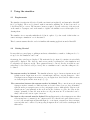
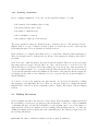
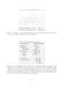
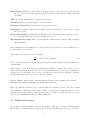
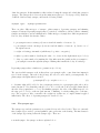
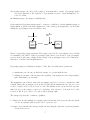
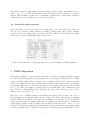
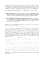
Spiking neural network simulator: User’s Guide
Version 0.55: December 7 2004
Leslie S. Smith, Department of Computing Science and Mathematics
University of Stirling, Stirling FK9 4LA, Scotland
[email protected]
1
Aims
The overall aim of this piece of software was to provide a general purpose simulator for spiking
neural networks. As such, it had to include
• the ability to take external spiking input
• the ability to save its spike output (for later inspection, and for possible re-use as input)
• the ability to be able to display spikes
• the ability to have multiple synapses between neurons with different delays
• some capability for adaptation
The aim was to concentrate on the spiking aspects: in particular we did not want to
• have complex (non-point) neurons
• model below the level of synapses themselves
Since the simulator was intended for use in conjunction with output from sound produced by the
MATLAB system, some degree of efficiency was important. In particular, we needed to be able to
model systems with a few thousands of neurons, and a few 10’s of thousands of synapses.
In its current state, the simulator provides all the above. It is intended as a research tool for
investigating spiking neural systems, and particularly their use in spike based auditory processing.
The basic mode of operation is very simple: once the network has been set up and the input files
determined, the network is simulated using a fixed time-step for a predetermined length of time.
The user can then choose to save spikes etc., or to alter the display, or to try out a different set of
inputs or synapses, and run the system again.
1
2
2.1
Using the simulator
Requirements
The simulator is written in Objective C (with some functions in plain C), and runs under MacOSX
10.3.5 (or higher). There are no plans to make it run under anything else. It has been tested on
both G4 and G5 processors. The amount of memory required depends on the size of the network,
on the number of synapses, and on the number of spikes: the simulator stores all its spikes before
drawing them.
The simulator is not currently multi-threaded (but it ought to be). One result of this is that one
cannot interrupt a simulation once it has started.
This document assumes that the reader is familiar with running applications under MacOSX.
2.2
Getting Started
Because this is a general purpose spiking neural network simulation, a number of things need to be
set up before the simulation can be run.
On startup, three windows are displayed. The main window (see figure 1) contains a view in which
spikes will be displayed. The other two windows are panels for parameters for the simulation and
for adaptation (see figures 2 and 4). These parameters may be entered directly: in addition, some
values may be saved and reloaded (see later). Before a simulation can be run, three things need to
be defined:
The neurons need to be defined The simulation has two types of neurons, input neurons, and
(plain) neurons. Input neurons receive external input, and have outgoing synapses to other
non-input neurons. Input neurons may not receive input from other neurons. Other neurons
are leaky integrate-and-fire neurons (see [5, 3]).
The connections between the neurons need to be defined These connections are the synapses.
Synapses can have a number of different forms, as described later: however, they all transfer
spikes from the pre-synaptic neuron to the postsynaptic neuron. Although the delay in a real
neural system occurs primarily at the axon and at the dendrites, we place the delay at the
synapse, primarily because the neurons here are all point neurons. Note that there can be
many connections between a pair of neurons.
The input to the network must be defined External input arrives only at input neurons. Other
neurons may have a constant (“tonic”) input as well. Note that if it is required that a neuron
receive both external input and internal input (i.e. tonic input or input from other non-input
neurons), this can be achieved by interposing an input neuron between the actual input and
this neuron.
2
2.2.1
Running a simulation
Prior to running a simulation, one needs to use the panel shown figure 2 to define
• the duration of the simulation (in seconds)
• the (fixed) timestep (in seconds)
• the number of input neurons
• the total number of neurons
• the parameter values up for the neurons
The neuron parameter values are discussed in more detail in section 2.3. The system is set up to
initialise itself to no noise. If this needs altered, then one should enter non-zero values into the
fields using this panel. Noise is discussed in detail in section 4.
If the system is to be adaptive, then values need to be entered into using the panel shown figure 4.
These are discussed in more detail in section 3. If none of the synapses are adaptive, these may be
left blank.
Next one needs to define the input to the network, and the synapses. These are set up by selecting
files using Spikes:Set simple spike file (there are other options as well: see section 2.5), for the
spikes, and Synapse: Set Synapse File for the synapses (see section 2.4). One can now press the Set
up network button in figure 1, to set up the network. This reads in the files, and creates various
objects and data-structures inside the simulation. The names of the spike file and the synapse file
are displayed in the window. Once this has been done, one presses the Start button in figure 1 to
run the simulation.
To look more closely at the spikes in some time interval, one can select the interval by clicking
and dragging to the right inside the view. Then one can press Redisplay to display this interval
using the whole of the View. It is not currently possible to display only a subset of the (non-input)
neurons.
2.3
Defining the neurons
Neuron definitiuon is achieved in either two or three stages. First, the number of input neurons and
the total number of neurons are set using the panel shown figure 2. There is no enforced minimum
or maximum (though obviously the total number of neurons must equal or exceed the number of
input neurons). Neurons are numbered from 0, starting with the input neurons. Secondly, the
default (non-input) neuron is characterised, also using this panel. The values (see figure 2) provide
the following information.
zero level The value to which the activity is set after a spike (normally 0).
3
Figure 1: The main view of the spiking neural network. Note that the vertical size of spikes drawn
depends on the number of spiking neurons being displayed.
Figure 2: The neural networks parameters panel, used for setting the duration and timestep for the
simulation, and for defining how many neurons are present. It is also used for defining the default
non-input neuron, and for determining whether all spikes should be kept and displayed, or whether
only those from non-input neurons should be kept and displayed, and for setting up the noise
level(s). Note that the simulation parameters, default neuron parameters and noise parameters can
also be saved to files, or read from files from the main menu.
4
Initial Ph(ase) The value of the activity at startup. If set to 0, then the neuron will start with
the zero level for its activity. Otherwise, this can allow the neuron to have a different activity
at startup.
Tonic A constant input applied to all neurons. 0 if none.
Threshold The level at which a spike occurs. Normally 1.
Ref(ractory) Period The neuron’s refractory period in seconds.
Dissipation A measure of the neuron’s leakiness. Defined as 1/RC (i.e. 1/τ ). If set to 0 then
there is no leak.
Sq(are) Diss’(ipatio)n A different form of leakage based on the square of the activity (see below).
For a leaky integrate-and-fire neuron, it should be set to 0.
Min’(imu)m Activ’(atio)n The lowest level that the activation may reach as a result of synaptic
input. Usually 0.
These values may be saved using Neurons: Save default neuron parameters, or loaded using Neurons:
Load default neuron parameters.
The activity of the neuron evolves according to
dA
= −D1 A − D2 A2 + input(t)
dt
(1)
where A is the activation, D1 is the dissipation, D2 is the square dissipation, and input(t) is the
external input.
In the absence of any other instructions, all the neurons will be identical. It is possible to use a
neuron file (with extension .neurons) to allow each (non-unput) neuron to have its own parameters.
The file can be chosen using Neurons:Set non-default neuron parameter file. Each line of this file
describes the parameters for one neuron. The file format is
<neuron number> <zero level> <initial phase> <Tonic value> <Refractory Period>
<Dissipation> <Square Dissipation> <Minimum Activation>
where each value is as described above, and the values are separated by tabs. The effect is that
the parameters for that neuron are changed. Thus, one can use the default parameters for some
neurons, and set other values for some other neurons, or, if required, set different values for every
neuron. Note that input neurons do not have parameters.
2.4
Defining the synapses
It is possible to run the simulator without any synapses. This can be useful for displaying spike
files: in this case, all the neurons are input neurons. To run a useful network, however, one needs to
5
define the synapses. In this simulation, this is achieved using the synapse file, which has extension
.synapse. The synapse file is chosen from the main menu (Synapses: Set Synapse File). Each line
of this file defines a single synapse, and has the following format:
<synapse type>
<synapse parameters>
There are three different types of synapse: plain synapses, depressing synapses and shunting
synapses. Plain and depressing synapses may be excitatory or inhibitory, and are additive: shunting
synapses are inhibitory, and are multiplicative. Different types of synapse have different parameters:
however, they all share the first five values:
1. pre-synaptic neuron: an integer (between 0 and the number of neurons - 1)
2. post-synaptic neuron: an integer (between 0 and the number of neurons - 1), but not one of
the input neurons.
3. weight: a floating point number (which may be positive or negative)
4. alpha: a positive number describing the value of α, for use in the alpha function (see below)
5. delay: a positive number determining the delay inherent in the path from the pre-synaptic to
post-synaptic neuron through this synapse. Making this 0 makes the delay one timestep.
Depressing synapses have a further two parameters (see below).
The way in which synapses work is that when a pre-synaptic spike occurs, that time instant is
stored at the synapse. After the delay (if any), the effect becomes visible post-synaptically. For
plain synapses an alpha function is used:
postsynaptic(T + t) = weight ∗ α ∗ t ∗ e−αt
(2)
to determine what will be added to the postsynaptic activity for a presynaptic pulse whose effect
started at time T . Note that this peaks at t = 1/α. If α = 0, the whole effect is applied immediately
after the delay (equivalent to α = ∞). For shunting synapses, the effect of the shunt is spread over
the time period of 3.0/α, with an equal amount of shunting of activity taking place each timestep. The exception to this occurs where the weight is 0: in this case, a complete shunt is applied
immediately. The effect of depressing synapses is described below.
2.4.1
The synapse type
The synapse type and the parameters are separated from each other by tabs. There are currently
three synapse types, and two optional qualifiers, put together into a short string. The first character
of the synapse type string defines the synapse type. These are:
s normal synapse: the synapse works as explained above
6
d depressing synapse: the effect of the synapse post-synaptically to a train of pre-synaptic spikes
decreases (equivalent to the depletion of a pre-synaptic reservoir of neurotransmitter). See
below for details
m shunting synapse: the synapse is multiplicative.
Both normal and depressing synapses may be excitatory or inhibitory, but the shunting synapse is
always inhibitory (in the sense that it shunts some of the activity post-synaptically to ground, thus
making the post-synaptic neuron less likely to fire).
Presynaptic
spike
Manufacture rate
Presynaptic
reservoir
postsynaptic
Utilisation
Figure 3: Depressing synapse schematic. The synapse is modelled by a presynaptic reservoir which
is continually being refilled. When a presynaptic spike arrives, some fraction of the presynaptic
reservoir is used, and causes a change in the activity of the postsynaptic neuron. Note that in use,
this may be combined with an alpha function.
Depressing synapses are illustrated in figure 3. They have an additional two parameters:
6. manufacture rate: the rate at which the synapse recovers strength after use
7. utilisation: a measure of the amount of the capability of the synapses used at each presynaptic
spike. This must be non-negative
The manufacture rate is linear: that is, the presynaptic reservoir recovers at a constant rate, until
it is full. Thus, if the presynaptic reservoir was 50% full, and the manufacture rate was 4, recovery
would be complete in (1 − 0.5)/4 = 0.125 seconds. The utilisation factor is used as and exponent:
thus, if it were 0, the synapse would not be depressing. If it was set to 1, then the level of the
reservoir would drop by a factor of 1/e after each presynaptic spike.
The synapse type may also contain two qualifiers:
r if this is absent, then multiple pre-synaptic spikes add linearly. If it is present, then the arrival
of a new pre-synaptic spike stops the effect of previous ones.
a adaptive: if present then the synapse weight can alter using the spike time dependent plasticity
described in section 3.
7
These qualifiers may occur anywhere except the first character of the synapse type.
2.4.2
Saving the synapses
Synapses may be saved in a format from which they can be reloaded. To do this, choose Synapses:
Save Synapses. The ability to save synapses (either for later inspection, or for later re-use) is
particularly useful when some of the synapses are adaptive.
2.5
Defining the Input Spikes
Input to the input units is read from a file. However, to allow for the simulator to be used with
output from a number of different places, there are a number of file types. The simplest file type
(selected using Spikes: SetSimple Spike File) contains a set of name/value pairs (which are read
and stored, but not otherwise used, with one exception, the name/value pair nspikes, which must
be present), followed by the single word spikes. After that comes a sequence of values of the form
<neuron number> <spike time>
The spike times must be in non-descending order (it is permissible for a number of spikes to occur
at the same time). The number of spikes which will be processed is the lower of the actual number
of spikes, and the value associated with nspikes. This allows the user to work with a large spike
file, but only to process those spikes near the start of the file.
A second type of file based input is provided to deal with input generated from local MATLAB
programs. This form of input (selected using Spikes:Set Matlab Spike File) is used to provide a
two dimensional input array, where one dimension is a number of different frequency channels,
and the other is a number of different sensitivity levels (see [7]). Again, the file contains a set
of name/value pairs. These are read and stored, but not otherwise used, with three exceptions,
spikes, iterations and channels. The first is used as before. The expected number of input units is
iterations ∗ channels, and an error message is displayed if this is not the case. This is followed by
a set of spike events, each of the form
<Iteration number>
<Channel number> <spike time>
As before, the spike times must be in non-decreasing order. Currently, the mapping from iteration
and channel number to input neuron number is
In = iterations ∗ (Channel number − 1) + (Iteration number − 1)
(3)
This can easily be changed (see the code in method setInputSpikes: (NSString *)inputspikefile
in the Network object). (This should probably be an option available without recompilation!).
8
The third file format for input spikes is the same as that produced for spike output, This is a Cocoa
archive object: we do not know its internal format, except insofar as it is known to be relatively
efficient. This can matter, as there may be any number of input and/or output spikes. Input files
of this format are loaded using Spikes: Load Generated Spikes.
2.6
Saving the spikes generated
Spikes which have been generated can be saved using Spikes: Save Generated Spikes. These are
saved in a Cocoa Archive format, suitable for reading by this program. There is also a humanreadable form, selected using Spikes: Save Generated Spikes (Human readable). This saves spikes
in the same form as the simple spike input described above.
Figure 4: The panel used for setting up spike time dependent plasticity (STDP) parameters.
3
STDP Adaptation
If the synapse qualifier “a” is present, then the synapse is adaptive. Currently, all synapses which
are adaptive adapt in the same way: the parameters are set as in figure 4. The basic idea of STDP
is that presynaptic spikes which occur just before postsynaptic spikes lead to an increase in the
efficacy of the synapse (long-term potentiation, LTP), and presynaptic spikes which occur just after
postsynaptic spikes lead to a decrease in the efficacy of the synapse (long-term depression, LTD)
(see e.g. [1]). There are a number of issues in the way in which STDP can be implemented, and
part of the idea of this simulation was to investigate the effect of these differences. Some of these
differences are reviewed in [6, 4].
The basic concept of STDP is that the actual change in weight depends not just on the order of
the presynaptic and postsynaptic spikes, but also on the precise timing. The changes are maximal
when the difference in timing between the two is smallest. Conceptually, the idea is that the
excitatory synapse whose presynaptic spikes helped to push the postsynaptic neuron over threshold
is strengthened, and the excitatory synapse whose presynaptic spikes were just too late to do so are
weakened. The first issue is whether the weight change depends on a number of presynaptic spikes
for each postsynaptic spike, or just the one nearest before and after the postsynaptic spike. We call
9
the former “classic”, and the latter “nearest neighbour” (NN) following [4]. This issue arises for
both prospective LTP and LTD. The next issue is whether a single postsynaptic spike at a synapse
can be responsible for both LTP and LTD, or just for LTP (“LTP wins”). These parameters chosen
for all three of these issues are set using the radio buttons on the top left of the panel (figure 4).
The actual amount of the weight change needs to be computed. There are three factors here:
the time constant (Rate) (pre → post R, and post → pre R) This determines the inter-spike
timing (i.e. time between presynaptic spike and postsynaptic spike) that results in STDP.
Note that R, the rate constant could also be written 1/τ , where τ is the time constant.
the weight change constant (Dw) This sets the size of the weight change
whether the weight change is additive or multiplicative Additive changes simply increase
or decrease the weight by a fixed amount: multiplicative changes result in smaller changes as
the weight gets towards its minimum and maximum possible values. The form of the change
can be different for LTP and LTD.
In addition, we can set minimum and maximum values for weights. The defaults for these are 0
and 1. The weight change is set using
∆ = Dw eR(S1 −S2 )
(4)
for both LTP and LTD. Note that R, the rate constant and Dw , the weight change constant may be
different for LTP and LTD. For LTP, S1 is the time of the post-synaptic spike, and S2 is the time of
the presynaptic spike. For LTD, S1 and S2 are reversed. Note that (S1 − S2 ) is always positive. In
the implementation, STDP is not calculated if (S1 − S2 ) > 5τ . The actual weight change is ∆ for
the additive case. For the multiplicative case, we use (wmax − weight)∆ for LTP, and | weight | ∆
for LTD, where the weight is excitatory. Where the weight is inhibitory, | wmin − weight | ∆ is
used for LTD, and | weight | ∆ for LTP . wmax and wmin are set using the STDP panel. Where
α is nonzero, the amount of LTP is altered a little to take account of the delay due to the alpha
function. In this case,
∆ = Dw eτ |(S1 −S2 −1/α)|
(5)
This peaks when S1 − S2 = 1/α, reflecting the actual contribution of the presynaptic spike to the
postsynaptic unit.
The STDP panel also permits the user to determine whether weights should be allowed to change
sign. Clearly, this applies only to additive weights. Further, the user can permit weights which
reach 0 to stop being adaptive. This allows weights which have been gradually decreased to zero
to stay at zero. They then have no further influence on the simulation.
There is an open question as to whether STDP should be applied to inhibitory weights, and,
if so, what form it should take. Hebbian adaptation implies that LTP is applied to inhibitory
synapses which arrived before the postsynaptic neuron fires. It is not clear that this is reasonable.
By setting the anti-H(ebbian) button, the weight changes for inhibitory synapses will run in the
opposite direction. Actually, it may be that STDP should not be applied to inhibitory synapses
at all, and that option is available to the user by using the simple option of not making inhibitory
weights adaptive.
10
4
Noise
In the absence of any noise, the system is completely deterministic. It is often useful to know
whether a particular behaviour would still occur if there was noise in the system. In addition,
neurons are often described as noisy (though whether this occurs due to factors inside the neuron,
or due to the multiplicity of additional inputs that real neurons receive, both synaptically, and due
to the many neuromodulators surrounding the neuron is unclear).
The simulation permits noise to be injected into neurons. As the simulation stands, the same type
of noise (but not the same noise) is injected into all neurons. When the system starts up, the
noise levels are all set to 0. Noise is generated using a class called “Random”, written by Gregor
Purdy for NextSTEP in 1991, based on [2]. This software needs three seeds to start, and these are
initialised when the simulation starts using the time. New seeds can be chosen (which would mean
that different noise would be generated).
Three type of noise are available from the system.
Tonic noise Noise applied to the tonic (constant) input of the neuron.
Threshold noise Noise applied to the threshold of the neuron.
Activation noise Noise applied to the activation level of the neuron.
The noise levels are set on the panel in figure 2, and may be saved using File: save noise parameters,
and loaded using File: load noise parameters.
Tonic noise is generated by first generating a random number uniformly distributed on [−0.5, 0.5],
and then multiplying this by the tonic noise level chosen to produce a value NT . The actual tonic
value is then multiplied by 1−NT . Note that if the tonic level is 0, then the noisy tonic level will also
be 0. Threshold noise again works with a similarly generated random number, and this is multiplied
by the threshold noise level chosen to produce NTh . The actual threshold to use is then multiplied
by 1 − NTh at each time step, so that each instantaneous threshold level is independent of the one
before or after it. The activation noise is computed in a similar way. First NA is computed, then
the activation calculated (using the synaptic and tonic inputs, dissipation and squared dissipation),
and then this is multiplied by 1 − NA .
Non-warranty
This software was produced for research purposes, and is made available for others to use. Absolutely no warranty is made for this software, nor for any damage or other effect it may have. If you
do use it in your research, the source should be credited.
11
Acknowledgements
Some financial support was supplied by the UK EPSRC. The simulation has benefitted from useful
disucssions with many people, particularly Bruce Graham, Bill Phillips and Florentin Woergoetter.
References
[1] G. Bi and M. Poo. Synaptic modification by correlated activity: Hebb’s postulate revisited.
Annual Review of Neuroscience, 24:139–166, 2001.
[2] T.A. Elkins. A higly random random-number generator. Computer Language, 6:59–65, 1989.
[3] W. Gerstner and W. Kistler. Spiking Neural Models. Cambridge, 2002.
[4] E.M. Izhikevich and H.S. Desai. Relating STDP to BCM. Neural Computation, 15:1511–1523,
2003.
[5] C. Koch. Biophysics of Computation. Oxford, 1999.
[6] P.J. Sjostrom, G.G. Turrigiano, and S.B Nelson. Rate, timing and cooperativity jointly determine cortical synaptic plasticity. Neuron, 32:1149–1164, 2001.
[7] L.S. Smith and D.S. Fraser. Robust sound onset detection using leaky integrate-and-fire neurons
with depressing synapses. IEEE Transactions on Neural Networks, 15:1125–1134, 2004.
12