1
15 June 1999 - Issue 1.0
ATSR-1/2 User Guide
Edited by Chris Mutlow
from contributions by J. Murray, P. Bailey, A. Birks and D. Smith
A short guide to the ATSR-1 and -2 instruments and their data products
The Along Track Scanning Radiometer (ATSR) instruments are imaging radiometers that provide images of the Earth’s surface from space. ATSR-1 was launched in
July 1991 and operated until June 1996. ATSR-2 is the current operational instrument and went into operation in 1995. AATSR will be launched in the year 2000.
Data from these instruments are useful for scientific studies of the land surface,
atmosphere, clouds, oceans, and the cryosphere.
The purpose of this guide is inform potential data users about the capabilities of the
Along Track Scanning Radiometers (ATSR-1 and -2) and their data products.
If you already know about ATSR-1/2 and want find out how to order data please
turn straight to Section 2.0, “Getting ATSR-1 and 2 Data Products,” on page 4 of
this document.
1.0 Introduction
Each ATSR instrument has been designed for exceptional sensitivity and stability of
calibration which are achieved through the incorporation of several innovative features in the instrument design:
• use of low-noise infrared detectors, cooled to near-optimum temperatures (i.e.,
less than 95 K) by a Stirling cycle mechanical cooler;
• continuous on-board radiometric calibration of the infrared channels against two
stable, high-accuracy blackbody calibration targets and, in the case of ATSR-2
and AATSR, calibration of the visible and near infrared channels with an onboard visible calibration system;
• use of the multichannel approach to SST retrieval previously demonstrated by
the AVHRR instruments;
• use of the “along-track scanning” technique to provide two views of the surface
and thus an improved correction for atmospheric effects.
ATSR's field of view comprises two 500 km-wide curved swaths, with 555 pixels
across the nadir swath and 371 pixels across the forward swath. The nominal instantaneous field of view (IFOV) pixel size is 1 km2 at the centre of the nadir swath and
1.5 km × 2 km at the centre of the forward swath (see Figure 1, “ATSR-1/2 Viewing
1 of 29
Introduction
Geometry,” on page 2). Each pixel is the result of a 75 µs integration of the signal
from the scene.
This viewing geometry produces 500- km-wide, high-resolution infrared and, in the
case of ATSR-2 and AATSR, visible images of the Earth's surface from which sea
surface temperature maps and other geophysical products can be retrieved through
ground processing.
1.1
Along Track Scanning
Application of the along track scanning technique is the ATSR instrument’s most
innovative development. This works by making two observations of the same point
on the Earth’s surface through differing amounts of atmosphere; the “along track”
view passes through a longer atmospheric path and so is more affected by the
atmosphere than the nadir view (see Figure 1, “ATSR-1/2 Viewing Geometry,” on
page 2).
First, the ATSR views the surface along the direction of the orbit track at an incidence angle of 55° as it flies toward the scene. Then, some 150s later, ATSR records
a second observation of the scene at an angle close to the nadir.
By combining the data from these two views a direct measurement of the effect of
the atmosphere is obtained, which yields an atmospheric correction for the surface
data set which is an improvement on that obtained from a single measurement.
FIGURE 1.
ATSR-1/2 Viewing Geometry
ATSR
Instrument
Sub-satellite Track
55 deg
Nadir view swath
( 555 nadir pixels
1 km resolution )
Flight Direction
Forward view swath
( 371 along track pixels
1.5 km x 2 km resolution )
1.2
ATSR-1
ATSR-1 was launched as part of the payload of ESA’s ERS-1 satellite on 17th July
1991, and was the test-bed for the along track scanning concept. It carries infrared
2 of 29
ATSR-1/2 User Guide - Issue 1.0
Introduction
channels at 1.6, 3.7, 10.8 and 12.0µm, and has no visible channels. Routine ATSR-1
operations stopped when ERS-1 was put into hibernation in June 1996, but the
instrument is still capable of operation as, even after nearly 7 years of use, the signal
to noise performance of the detectors is higher than for a typical AVHRR at launch.
1.3
ATSR-2 and AATSR
The ATSR-2 and Advanced ATSR (AATSR) instruments are developments from
the original experimental ATSR-1 instrument which, in addition to the ATSR-1’s
infrared channels, carry extra visible channels at 0.55, 0.67 and 0.87µm for vegetation remote sensing. The evolution of ATSR-2 was constrained by the requirement
to maintain the ATSR-1 precision measurement of global SST.
The ATSR-2 instrument, launched in April 1995, is currently flying as part of the
payload of the ESA ERS-2 satellite, and AATSR will be launched early next century on ESA’s Envisat platform.The AATSR instrument represents an orderly development of the ATSR series of instruments. The ATSR channels are given in Table 1,
“ATSR-1, ATSR-2 and AATSR Spectral Channels,” on page 3
TABLE 1.
ATSR-1, ATSR-2 and AATSR Spectral Channels
Feature
Wavelength
Bandwidth
ATSR-1
ATSR-2
AATSR
Detector type
Chlorophyll
0.55µm
20nm
N
Y
Si
Vegetation Index
0.67µm
20nm
N
Y
Si
Vegetation Index
0.87µm
20nm
N
Y
Si
Cloud Clearing
1.6µm
0.3µm
Y
Y
PV InSb
SST retrieval
3.7µm
0.3µm
Y
Y
PV InSb
SST retrieval
10.8µm
1.0µm
Y
Y
PC CMT
SST retrieval
12.0µm
1.0µm
Y
Y
PC CMT
The ATSR-2 instrument for ERS-2 is largely the same as ATSR-1 except for:
• the inclusion of 3 extra spectral bands in the visible, mainly for vegetation monitoring;
• an on-board visible calibration system.
The AATSR instrument is functionally the same as the ATSR-2, but the structure
and some of the other components have been re-worked to match the environment
of the Envisat platform, which is somewhat different to the ERS satellites.
The major purpose of AATSR is to provide continuity of the crucial sea surface
temperature data sets which have been produced by ATSR-1 and ATSR-2. Therefore, the key scientific parameters which were optimised for ATSR, are retained for
AATSR. Thus details of the scan, the optical system, the basic spectral bands, thermal calibration system, spatial resolution and swath have been kept as close as possible to those of the original instrument to ensure continuity.
The major advantage AATSR has over ATSR-2 is in the telemetry bandwidth available on Envisat. For ATSR-2, the limited telemetry available on ERS-2 imposed
severe limitations on the collection of visible channel data; on Envisat there are no
ATSR-1/2 User Guide - Issue 1.0
3 of 29
Getting ATSR-1 and 2 Data Products
such restrictions, so AATSR can telemeter all the visible channel data it can collect.
This significantly simplifies the ground processing required for AATSR data, as the
processor does not need to cope with the wide range of data formats that are possible from ATSR-2.
2.0 Getting ATSR-1 and 2 Data Products
The following sub-sections describe how the various sections of the user community can order ATSR data sets and the services that are available to support browsing and selection prior to placing an order.
2.1
How do I find out what ATSR-1/2 data are available?
In addition to the information provided on the ATSR Project web pages there are
now new services that allow potential ATSR data users to view quick-looks of the
image data available through the various processing facilities prior to placing an
order for the full-resolution data sets.
2.1.1
NERC ATSR Browse Facility
To provide easy access to ATSR data the UK NERC has established a Browse Facility at RAL which provides on-line access to quick-looks of the entire ATSR-2
image data set, and is starting to be populated with ATSR-1 data set as well. Users
are strongly encouraged to make use of this facility to establish their data needs
before requesting data from either RAL or ESA.
Access to the facility can be gained directly via a link from the ATSR Project’s
home page at URL http://www.atsr.rl.ac.uk.
2.1.2
ESA Multi-Mission Browse Facility
ESA also has an ATSR browse service that can be reached at URL http://earthnet.esrin.esa.it.
2.2
Where do I order ATSR-1/2 data?
The following sub-sections describe where the various sections of the user community can place their order for ATSR-1/2 data products.
2.2.1
New Users
The ATSR Project Team at RAL are able to supply any “new user” with samples of
ATSR-1/2 data to get them started quickly with an ATSR data set appropriate to
their needs - this service is available through the ATSR Project at RAL at the
address in Section 2.2.2.
Following such an initial data grant the user will be referred to the appropriate data
centre as described below for any future requests.
2.2.2
NERC-funded UK Scientists and Validation Scientists
This category includes NERC Staff, holders of NERC-funded research grants or
thematic programme awards, and scientists providing validation data. These users
can obtain their data from the ATSR Project Team by submitting a NERC AT1
form. Further information on the procedure and the actual form can be found on the
ATSR project web pages at http://www.atsr.rl.ac.uk or by contacting
4 of 29
ATSR-1/2 User Guide - Issue 1.0
Data Products
Nigel Houghton, ATSR Project, Rutherford Appleton Laboratory, Chilton, Didcot,
Oxon, OX11 0QX, email [email protected].
2.2.3
Other Scientists and Commercial users
This category of users must obtain their data from ESA through the ERS Help Desk
at Esrin, in Frascati near Rome.
The contact details for ATSR data through ESA are:ERS Help Desk, via Galileo Galilei, CP. 64, 0044 Frascati, Italy
Phone:+39-06-94180-666 Fax.: +39-06-94180-272
E-mail: [email protected]
ESA Browse Service: http://earthnet.esrin.esa.it
These data are processed on behalf of ESA by NRSC Ltd. at Farnborough who are
the official ESA processing and archiving facility for the ATSR instrument.
2.2.4
Near-Real-Time Users
In recent weeks a new near-real-time service for ATSR-2 data products has come
into operation at the Tromsø Satellite Station. The web address for accessing this
service is http://192.111.33.173/ATSRNRT/. There is direct access the quick-look
images archives, but users have to register with ESA to if they wish to access the
full-resolution data sets.
3.0 Data Products
All ATSR-1 and -2 data from whatever source are processed using SADIST (Synthesis of ATSR Data Into Sea-surface Temperatures), the Rutherford Appleton Laboratory’s ATSR data-processing scheme (Závody et al., 1994).
Currently, two distinct versions of SADIST exist; ATSR-1 data were processed with
SADIST-1, and ATSR-2 data with SADIST-2. However over the last few months a
unified version of the software has become available, so in future ATSR-1 data will
be re-processed using SADIST-2 and be in a common format. Major enhancements
in the second version of the software include the capability to provide additional the
visible channel data, and more robust cloud identification and additional product
confidence data.
Full details of the ATSR product set are described in the ATSR product format
guides available from the ATSR Project Web Site (http://www.atsr.rl.ac.uk); separate guides cover the SADIST-1 and 2 product sets.
The set of SADIST-2 ATSR-1/2 products comprises three logical groups
Ungridded products contain pixels in the ATSR scan geometry (i.e., in the instrument frame of reference where the curved scans appear as straight lines and the surface scene is distorted). There is a direct correspondence between the contents of a
product record and the contents of an ATSR instrument scan. Nadir- and forwardview pixels in a record correspond to the same scan and are, therefore, not colocated.
ATSR-1/2 User Guide - Issue 1.0
5 of 29
Data Products
Gridded products contain 512 × 512 pixel images. The correspondence between a
pixel and the ATSR instrument scan from which it came has been lost. Nadir- and
forward-view pixels are collocated, and have been regridded (mapped) onto a 1 km
grid.
Spatially-averaged products have contents (derived from up to a whole orbit of
raw data) which have been spatially-averaged to a ten-arcminute or half-degree resolution.
3.1
Ungridded products
There are two ungridded products:
UCOUNTS is an ungridded detector count product. The product contains ungridded, uncalibrated detector counts from all or some of the ATSR-1/ATSR-2 detectors. Although the product remains ungridded, it may optionally contain pixel
latitude/longitude positions, and/or pixel X/Y (across-track/along-track) coordinates.
UBT is an ungridded brightness temperature/reflectance product (a new product for
SADIST-2). The product contains ungridded, calibrated brightness temperatures or
reflectances from all or some of the ATSR-1/ATSR-2 detectors. Although the product remains ungridded, it may optionally contain pixel latitude/longitude positions,
and/or pixel X/Y (across-track/along-track) coordinates.
3.2
Gridded products
There are three gridded products:
GBT is a gridded brightness temperature/reflectance product (an extension of the
SADIST-1 BT product). The product contains gridded, calibrated brightness temperature or reflectance images from all or some of the ATSR-1/ATSR-2 detectors.
The product optionally includes pixel latitude/longitude positions, X/Y offsets (subpixel across-track/along-track coordinates), and the results of cloud-clearing/landflagging.
GBROWSE is a gridded browse product (an extension of the SADIST-1 BROWSE
product). The product contains gridded, sub-sampled, calibrated brightness temperature or reflectance images from all or some of the ATSR-1/ATSR-2 detectors. The
product optionally includes the results of cloud-clearing/land-flagging.
GSST is a gridded sea-surface temperature product (an extension of the SADIST-1
SST product). The product contains gridded sea-surface temperature images using
both nadir-only and dual-view retrieval algorithms. The product optionally includes
pixel latitude/longitude positions, X/Y offsets (sub-pixel across-track/along-track
coordinates), and the results of cloud-clearing/land-flagging.
3.2.1
Spatially-averaged products
There are three spatially-averaged products:
ABT is a spatially-averaged brightness temperature/reflectance product (a new
product for SADIST-2). The product contains spatially-averaged brightness temper6 of 29
ATSR-1/2 User Guide - Issue 1.0
Data Products
atures/reflectances from all or some of the ATSR-1/ATSR-2 detectors, categorised
by view, channel, surface type and cloud-presence.
ACLOUD is a spatially-averaged cloud temperature/coverage product (unchanged
from the SADIST-1 ACLOUD product). The product contains spatially-averaged
measures of cloud temperature and abundance.
ASST is a spatially-averaged sea-surface temperature product (an extension of the
SADIST-1 ASST product). The product contains spatially-averaged sea-surface
temperatures, at ten-arcminute and half-degree resolution, using nadir-only and
dual-view retrieval algorithms.
In the spatially-averaged products generated by SADIST-2 the pixels which contribute to such products are taken from gridded (and therefore collocated) pixel data.
3.3
Optional product contents
The approach adopted by SADIST-2, to strike a balance between flexibility and
simplicity, is to split product contents into several significant categories. Each category is represented by a single letter code in product requests, and in product filenames. The combination of codes defines in a concise way the actual product contents. The product content categories are:
Nadir-view only (N): only those records containing nadir-view ATSR data. (Note
that this option is rather different from the others in that its presence indicates the
absence of product records: those containing ATSR forward-view data.)
Thermal infrared detectors (T): records containing the thermal infra-red/nearinfra-red (12.0µm, 11.0µm, 3.7µm, 1.6µm) channels, which are available from both
ATSR-1 and ATSR-2 instruments.
Visible detectors (V): records containing the visible/near-infra-red 1.6µm, 0.87µm,
0.65µm, 0.55µm channels, which are available from only the ATSR-2 instrument.
Pixel latitude/longitude positions (L): records containing precise Earth-locations
for ATSR instrument pixels.
Pixel X/Y coordinate positions (X): records containing precise pixel-locations (for
ungridded products), or sub-pixel offsets (for gridded products), in the across-track/
along-track coordinate system defined by the ERS platform trajectory.
Cloud-clearing/land-flagging results (C): records containing the detailed results
of cloud-clearing tests and pixel land-flagging.
It should be noted that not every category is available for each product type, so not
all product options are always available. For each product, and for each instrument
type (ATSR-1, ATSR-2) there is a default product; such default products have been
chosen to satisfy most product users, whilst minimising product size.
Note also that the ACLOUD and ASST products have no optional contents. Since
their product sizes are relatively small, and the contents are valid for both ATSR-1
and ATSR-2 instruments, flexibility provides no benefit.
ATSR-1/2 User Guide - Issue 1.0
7 of 29
Data Products
3.4
Portability, byte-ordering and the byte-order word
In designing the ATSR products, it has been attempted to keep the products as portable as possible between operating systems and languages. To this end:
• The products contain no floating-point numbers. Only ASCII text (within product headers), and one-, two-, and four-byte integers are used throughout the products.
• The products contain fixed-length records. This provides portability between
record-based operating systems, such as OpenVMS, and stream-based operating
systems, such as UNIX.
However, an intrinsic difference between systems remains. Some systems interpret
the bytes within integers such that the bytes are given increasing significance,
whilst others interpret the bytes within integers such that the bytes are given
decreasing significance. SADIST-2 is a VMS application. Since VMS is a littleendian system, the bytes within two-byte words and four-byte words are stored in
increasing order of significance. If SADIST-2 products are to be read on big-endian
systems, the byte-ordering must be reversed. That is, the internal representation
must be changed so that the intended value will be retrieved.
To provide a mechanism whereby the process of byte-swapping might be automated, the first two bytes within each SADIST-2 product header are fixed, and can
be used to test the byte-ordering on the local system.
3.5
Visible channel normalisation
No routine calibration is performed on the visible and near-infrared image data supplied to users from SADIST-2, instead this must be done explicitly by the user with
the calibration tables provided on the ATSR Project Web site (http://
www.atsr.rl.ac.uk). The visible and near-infrared data provided in the SADIST
product are in the form of raw uncalibrated telemetry but they have been normalised
to lie within a given range.
The normalisation procedure applied to each of the visible channels, including the
1.6µm near-infrared channel, to achieve this is:
1. The channel offset has been removed.
2. The channel gains have been normalised to account for variations in the signal
channel processor (SCP) gain setting.
Thus, in SADIST-2 products which contain visible channel signals (UBT, GBT,
GBROWSE, ABT), the visible channels have been normalised to SCP gains of 20.
That is, the signals are those which would have been generated by the instrument if
SCP gains of 20 were being used. Table 2 on page 9 shows the actual nominal SCP
gains used (for ATSR-2), and the effective increase in signal due to the normalisation procedure. Note that since the gains have been commanded to give a full-scale
uncalibrated count (4095) during the day-time peak, the approximate normalised
8 of 29
ATSR-1/2 User Guide - Issue 1.0
Ground segment data processing
maximum in each case represents the signal during the day-time peak, and not
100% reflectance.
TABLE 2.
ATSR-2 normalised visible channel signals
Channel
Nominal SCP gain
Normalised gain
Approx. normalised range
1.6µm
3.79
20.0
0 – 21108
0.87µm
3.73
20.0
0 – 21447
0.67µm
3.10
20.0
0 – 25806
0.56µm
4.38
20.0
0 – 18264
Once, as here, the offsets and gains have been removed and normalised respectively, the only part of the calibration of the visible channels which remains is
applying 100% reflectance scaling factors to convert normalised counts into true
top-of-atmosphere reflectances. Such scaling factors are the product of RAL’s characterisation of ATSR-2’s VISCAL unit; see “Visible and near-infrared channels” on
page 12 for details their derivation and application. The calibration tables themselves can be found at the following URL http://www.atsr.rl.ac.uk/calibration.html.
4.0 Ground segment data processing
4.1
Introduction
ATSR-1 and -2 data cannot be received directly from the satellites by users because
there is no continuous direct broadcast of data from either ERS-1 or -2. Instead, the
ATSR data collected each orbit, together with the low bit rate data from the other
sensors on the platform, are stored on an on-board tape recorder for subsequent
transmission to the ground. These stored data are then transmitted to the ground
during each orbit when the satellite is within the reception range of one of the designated ESA ground stations which are at Kiruna, Sweden; Maspalomas, Canary
Islands; Gatineau and Prince Albert, Canada. (Kiruna is the main station receiving
10 out of the 14 orbits of data collected each day.)
No real-time data is lost during the tape recorder playback because the satellite
operates two simultaneous data links, meaning that the current payload data can be
transmitted as it is collected without affecting the tape recorder dump. The real-time
data and the tape recorder dump are merged together duringprocessing at the ground
stations. It should be noted that the combination of tape recorder capacity and
acquisition time at the ground station is a limitation during some ERS orbits, this is
explained further in “Descoping” on page 23. The data received at the ESA stations
are then subsequently supplied to the various processing facilities on Exabyte tapes.
The two centres which process the ATSR-1 and 2 data are in the UK Processing and
Archiving Facility (UK-PAF) at the National Remote Sensing Centre (NRSC) in
Farnborough, UK, and the ATSR Project Team at the Rutherford Appleton Laboratory, UK. Each of these facilities serves a different set of ATSR data users:1. The UK-PAF at NRSC is the official ESA Processing and Archiving Facility
(PAF) for ATSR and, therefore, supplies image data to the international science
community, non-NERC funded UK scientists, and commercial users.
ATSR-1/2 User Guide - Issue 1.0
9 of 29
Ground segment data processing
2. The ATSR Project Team at RAL generates the spatially-averaged climate prod-
ucts from ATSR-1 and -2, and also provides a comprehensive ATSR image data
service to NERC-funded UK scientists. It also has a mandate to provide low volumes of sample products to any new user of ATSR data who applies, and to provide data for validation purposes.
Figure 2 shows the flow of ATSR-1 and 2 data from the satellite to the user community.
FIGURE 2.
Schematic showing the distribution chain for ATSR-1 and 2 data
Data transmitted to
ESA Ground Stations
Prince Albert
Maspalomas
Gatineau
Kiruna
Raw data sent to
processing centres
on Exabyte tape
Raw data on Exabyte
Data processed in one of
two UK centres which each
serve different types of user
UK PAF
ATSR Project Team
NRSC
RAL
ESA-Funded
Processing Facility
ESA PIs
Commercial Users
non-NERC Funded UK Scientists
NERC-Funded
Processing Facility
NERC Funded UK Scientists
New Users
Instrument Consortium partners
The limitation of both of these facilities is that they can only offer off-line ATSR-1/
2 product generation services and supply data to the community 7-14 days after its
original collection at the earliest. Such a delay is too long for many users. Therefore, ESA have developed a pilot ATSR near-real-time processing system which is
now in operation at the Tromsø Satellite Station (TSS). By agreement (and because
of its geographic proximity), this station can eavesdrop on the 10 orbits of satellite
data downlinked to the Kiruna station each day, and processes this data in near-realtime to deliver ATSR-2 products to real-time users. The spatially-averaged products
from this system are now being supplied to the meteorological community, and
other customers get access to this data and can also order image products from TSS.
4.2
4.2.1
4.2.1.1
Data Processing Algorithms
Calibration
Infrared channels
The signal in counts from a radiometer channel observing a blackbody target at temperature Tbb is
10 of 29
ATSR-1/2 User Guide - Issue 1.0
Ground segment data processing
S ( T bb ) = GL ( T bb ) + S 0
(EQ 1)
where G is the radiometric gain, L(Tbb) is the radiance from a target (i.e. the Planck
function integrated over the filter passband), and S0 is the radiometric offset of the
channel.
Radiometric calibration of the instrument consists of determining the linear relationship between the radiance and detector counts from each channel. The conventional way of doing this is to allow the instrument to view a zero radiance target,
such as a cold space view, to determine the radiometric offset S0 (i.e., L(Tbb) = 0).
Then having determined S0, the radiometer views a hot calibration target to determine the radiometric gain of the channel. Then the gain of the system is given by
S cold – S 0
G = --------------------L cold
(EQ 2)
In “real” radiometers there is always some degree of non-linearity which, if not
treated properly in the ground processing algorithms, results in errors in calibration.
This is a particular problem if the non-linearity changes with time.
To avoid these problems as far as possible, the approach adopted in the ATSR
instruments has been to minimise the sensitivity of the calibration to any non-linearity in the radiometer's characteristics. This has partly been done by careful design of
the signal processing electronics and by careful pre-flight determination of the nonlinearity for “beginning-of-life” and “end-of-life” conditions on the satellite, but
mainly through designing the calibration system in such a way that the instrument's
on-board calibration is optimised over the limited range of temperatures that span
the expected range of SST observations.
ATSR uses two blackbody calibration targets, rather than the more usual single hot
target and a space view. In ATSR one of these targets operates at a temperature
cooler than the coldest expected SST, and the other one warmer than the hottest
expected SST.
With this arrangement the calibration is most precise over the temperature range
covering the normal range of SST. The effects of any non-linearity in the system are
minimised because linearity is only assumed over a small range of measurement
space. Outside this range, the calibration is no worse than using the space view and
single calibrator approach, but using the ATSR method the precision is concentrated
into the portion of the measurement space where the most accurate measurements
are required. At temperatures outside this range the precision of the observations are
not so critical, and the larger calibration errors resulting from extrapolation can be
tolerated.
The scheme used for determining the ATSR instrument’s calibration parameters
from the hot and cold blackbody signals is given below.
ATSR-1/2 User Guide - Issue 1.0
11 of 29
Ground segment data processing
The signal from ATSR’s cold blackbody is given by
Scold = GL cold + S 0
(EQ 3)
and the signal from the hot blackbody is given by
S hot = GL hot + S 0
(EQ 4)
Hence, by subtracting the above equations to eliminate S0, the radiometric gain G is,
S hot – S cold
G = -------------------------L hot – L cold
(EQ 5)
and by substituting G back into the equations the offset S0 is,
S 0 = S hot – G L hot
(EQ 6)
The infrared focal planes of the ATSR instruments use two different types of infrared detectors;
1. the 1.6 and 3.7µm channels employ photovoltaic indium antimonide (InSb);
2. the 10.8 and 12.0µm channels use photoconductive cadmium mercury teluride
(CdHgTe or CMT) detectors.
The response of the InSb detectors is fairly well behaved and linear over the range
of temperatures from liquid nitrogen to 310 K.
The same is not true of the CMT detectors, which show a marked non-linear behaviour because of “Auger recombination”. This causes a reduction in the measured
detector signal at high photon fluxes compared to that predicted assuming a linear
detector response. The size of this reduction depends on the temperature and
decreases as the detector temperature increases.
The non-linear detector responses are corrected using the measured radiances from
the pre-flight calibration and characterisation.
4.2.1.2
Visible and near-infrared channels
Visible channel calibration is achieved in a similar way to the infrared channels.
Careful pre-flight calibration and characterisation of the visible channels was performed, and this is supplemented by continuous in-flight calibration of the channels
with an on-board visible calibration system.
The radiometric offset for the visible channels is determined by viewing the ATSR2 cold blackbody. The signal measured while viewing this target is assumed to be
the “dark signal” for the channels (i.e., the signal observed by a blinded detector).
12 of 29
ATSR-1/2 User Guide - Issue 1.0
Ground segment data processing
The radiometric gain is determined once each orbit when the instrument’s visible
calibrator is illuminated by the Sun as the satellite moves away from the South pole.
At this point sunlight enters the VISCAL baffle through a protective window and is
directed onto a Russian opal diffusing plate. This plate is seen by the instrument
scan mirror as a bright patch at the edge of the hot blackbody during each scan. The
VISCAL provides a radiance equivalent to a 25% signal from a Lambertian scatterer. The performance and degradation of the VISCAL is monitored by a photodiode.
The gain G vis of the visible channels is therefore given thus,
S viscal – S dark
G vis = ------------------------------L viscal
(EQ 7)
where S dark is the radiometric offset derived from the internal blackbody views,
S viscal is the signal from the ATSR-2 VISCAL unit, and L viscal is the solar radiance
from the VISCAL.
These calibration data are not used directly within SADIST-2 to calibrate the data
from the visible and near-infrared channels; it is left to the user to do this using the
calibration tables provided at the URL http://www.atsr.rl.ac.uk/calibration.html.
These tables are updated on a regular basis using the method described above.
Users are reminded that some care is required to ensure that up-to-date calibration
information is used as trend plots reveal oscillations in short wavelength signal
intensity caused by a build up of condensation on a relay lens mounted on the cold
focal plane assembly (FPA). This is accounted for by the calibration procedure, and
has a negligible effect on accuracy if the correct set of calibration coefficients are
used. Care must also be exercised if data from an outgassing period is used as the
calibration becomes undefined while an outgassing is underway owing to rapid
changes in the condensate film thickness as it evaporates.
If you are in any doubt over the use of the calibration data please contact the ATSR
Project Team at RAL who will be able to advise on the correct procedure, and also
on the status of the instrument.
4.2.1.3
General Points on Calibration
It should be noted that, although it is not explicitly mentioned elsewhere, odd and
even pixels from the sensor are calibrated separately as they are obtained from different integrators. In the current version of the ATSR software this may not always
be done correctly in “jittered” scans (see Section 6.2.4 on page 27); a fix is available and will be included in a later update.
4.3
Geolocation and regridding
ATSR SADIST image products betray no sign of the fact that the ATSR instruments
possess a conical scan mechanism, which results in the acquisition of nadir- and forward-view pixels many hundreds of kilometres apart, and which possess a curved
geometry. It is an important part of the data-processing within SADIST-2 to remove
such spatial view-differences and scan geometry by performing pixel geolocation
ATSR-1/2 User Guide - Issue 1.0
13 of 29
Ground segment data processing
(the derivation of the Earth-locations of the acquired pixels) and view collocation
(the process by which, assuming the geolocation is sound, the nadir and forward
views are spatially matched).
The geolocation proceeds by mapping the acquired pixels onto a 1 km grid whose
axes are the ERS satellite ground-track and great circles orthogonal to the groundtrack. The resampling is done using a nearest neighbour method, and the actual X/Y
co-ordinates of a given pixel are retained in the gridded products. This regridding
has two effects. Pixels which are small, and whose Earth-locations are therefore
very small, may be placed within the same 1 × 1 km box (in which case the first is
overwritten). Also, some pixels in the regridded image may remain unfilled. This
unfilling occurs when pixels are large, and consequently further apart than 1 km.
All latitudes provided within SADIST-2 products are geodetic; that is, they show
the angle formed by the intersection between the equatorial plane and the local normal at the Earth’s surface.
4.3.1
Cosmetic fill
Grid pixels which remain unfilled by the regridding process are filled by copying
the nearest (“real”) neighbour. It can be seen that this process of cosmetic-filling has
the effect of (approximately) reconstituting original pixel sizes. Filling occurs only
where actual pixels are large, and therefore widely-spaced, but have been squeezed
into 1 × 1 km boxes. Nearest-neighbour copying reverses the pixel squeezing, and
allows pixels to expand to a more representative size.
4.3.2
Cloud Clearing
The process of cloud-clearing, or the identification of “clear” pixels, is accomplished by applying in turn a series of tests to the brightness temperature data in the
12, 11 and 3.7µm channels, and to the reflectance data in the 1.6µm channel.
The pixel is flagged as cloudy if any one of the tests indicates the presence of cloud.
Considered in detail, the physics involved is complicated; however, broadly speaking the detection of cloudy pixels is based upon identifying deviations caused by the
presence of cloud from the properties of and relationships between measured brightness temperatures expected for clear conditions. (See Závody et al. (1999) for more
details of the ATSR cloud clearing scheme.)
Table 3 below summarises the cloud clearing tests implemented in SADIST. All of
the tests are of course conditional on the appropriate infrared or 1.6µm data being
available. The 1.6µm test operates on daytime data only. The tests involving the
3.7µm channel, on the other hand, are only applied to night-time data, because
reflected solar radiation may be significant in this channel during the day. Those
tests that involve the 11 and 12µm channels are applicable to both daytime and
14 of 29
ATSR-1/2 User Guide - Issue 1.0
Ground segment data processing
night-time data. Not all of the tests are implemented over land so cloud clearing
over land is not as effective as over the ocean.
TABLE 3.
ATSR cloud clearing tests
Cloud Test
Views used
1.6µm histogram test
nadir and forward views
11µm spatial coherence test
nadir and forward views
Gross cloud test
applied to nadir and forward views separately
Thin cirrus test
applied to nadir and forward views separately
Medium/high level cloud test
applied to nadir and forward views separately
fog/low stratus test
applied to nadir and forward views separately
11/12µm nadir/forward test
uses both views
11/3.7µm nadir/forward test
uses both views
Infrared histogram test
applied to nadir and forward views separately
A series of cloud state flags is defined within the SADIST code for each pixel and
for the forward and nadir view separately. These are listed in Table 4.
TABLE 4.
Cloud-clearing/land flagging flag bit settings (nadir or forward view)
bit #
Meaning if set
0
Pixel is over land
1
Pixel is cloudy (result of all cloud tests)
2
Sunglint detected in pixel
3
1.6µm reflectance histogram test shows pixel cloudy (day-time only)
4
1.6µm spatial coherence test shows pixel cloudy (day-time only)
5
11µm spatial coherence test shows pixel cloudy
6
12 µm gross cloud test shows pixel cloudy
7
11/12µm thin cirrus test shows pixel cloudy
8
3.7/12µm medium/high level test shows pixel cloudy (night-time only)
9
11/3.7µm fog/low stratus test shows pixel cloudy (night-time only)
10
11/12µm view-difference test shows pixel cloudy
11
3.7/11µm view-difference test shows pixel cloudy(night-time only)
12
11/12µm thermal histogram test shows pixel cloudy
These flags are set according to the results of the tests. Thus if one of the flags numbered 3 to 12 is set, this means that the corresponding test has indicated the presence
of cloud. If on completion of the cloud-clearing sequence any of these flags is not
set, it may mean either that the test did not indicate the presence of cloud, or that the
test was not applied because suitable data was lacking.
4.3.3
SST retrieval
The objective of this procedure is to use the measured infrared brightness temperature values to determine, for each cloud-free pixel over sea, the best estimate of the
ATSR-1/2 User Guide - Issue 1.0
15 of 29
Ground segment data processing
Sea Surface Temperature (SST) of the pixel, to form an SST image at 1 km resolution.
The SST is calculated using predetermined coefficients. In the current version the
coefficients are given for three geographical regions: tropical, midlatitude and polar.
(A new version is under test which use a global set of coefficients.) The values of
the coefficients also depend to some extent on the viewing angle, and so the acrosstrack distance of the pixel expressed in terms of band number determines the set of
coefficients to be used for a given pixel. In the current version five different sets of
coefficients are defined for each geographical region, to represent the 5 different
across-track distances (and therefore air masses) corresponding to the across-track
bands. There are thus 15 sets of coefficients for each case.
Whenever possible, both the nadir view and forward view pixels are used. Cloud
contamination for the forward view pixels is more likely than for the nadir view due
to the larger sampling area in the former, hence the possibility of using the brightness temperatures from the nadir view only is also catered for. (It would be possible
in theory to derive retrieval coefficients for the case of a forward view image only,
but this is not done in practice.)
The algorithms using the nadir view only are given by
= a0 + a1Tirnadir
+ a2 Tirnadir
Tsstnadir
,i
11
12
(EQ 8)
or
= b0 + b1Tirnadir
+ b2 Tirnadir
+ b3Tirnadir
Tsstnadir
,i
11
12
37
(EQ 9)
When both views are used, the corresponding equations are
= c0 + c1Tirnadir
+ c2 Tirnadir
+ c3Tirfrwrd
+ c4 Tirfrwrd
Tsstdual
,i
11
12
11
12
(EQ 10)
or
= d 0 + d1Tirnadir
+ d 2 Tirnadir
+ d 3Tirnadir
+ d 4 Tirfrwrd
+ d5Tirfrwrd
+ d 6Tirfrwrd
Tsstdual
,i
11
12
37
11
12
37
(EQ 11)
respectively.
If the pixel is over land an SST retrieval is clearly not appropriate. In order to provide a precision estimate of the land surface temperature it would be necessary to
have detailed information about the emissivity of the land surface in the various
channels. This would present some difficulty given the large spatial variability in
the physical characteristics of land surfaces. In this case therefore, SADIST supplies
the 11µm nadir-view brightness temperature as the best available estimate of the
land surface temperature in the absence of such detailed information.
The logic of the procedure used within SADIST for deriving a retrieved SST is
therefore as follows in Figure 3 on page 17.
16 of 29
ATSR-1/2 User Guide - Issue 1.0
Ground segment data processing
When a dual view retrieval is required, the procedure is similar except that the 11
and 12µm brightness temperatures for both nadir-view and forward view must be
checked for validity. If all four are valid, the solar elevation and 3.7µm brightness
temperatures for the image pixel in both views are inspected. If both brightness temperatures are valid and the solar elevation is negative for both views, a 3-channel
retrieval is made, otherwise a two-channel retrieval is performed. As before if one
of the 11 or 12µm brightness temperatures is invalid, the “forward view SST valid”
flag is set to false (again it is initialized to this value) and the retrieved temperature
is set to the 11µm nadir-view brightness temperature.
In theory SSTs should not be calculated for cloudy pixels. If both views (forward
and nadir) are cloud-free, then clearly a valid dual-view retrieval is possible, and if
the nadir view is cloud-free a valid nadir-view retrieval is possible. However, if the
nadir view pixel is cloudy, or if both views are cloudy, a valid retrieval is not possible for either the nadir view or dual view cases. Nevertheless, in SADIST both nadir
and dual view retrievals are derived in all cases where the pixel is over the sea, and
the interpretation is left to the user, who of course has available the cloud identification flags in the confidence word.
FIGURE 3.
Schematic of the decision flow in the ATSR SST retrieval algorithm
Pixel data
Diagram showing the decision
flow in the ATSR SST retrieval
algorithm
Is the pixel over
sea ?
No
Set result to the
11µm BT value
No
Set result to the
11µm BT value
Yes
Are the 11µm &12µm
BTs valid ?
Yes
Is it night time ?
No
Use 2-channel
retrieval scheme
11µm &12µm BTs
Yes
Is the 3.7µm BT
No
valid ?
Yes
Use 3-channel
retrieval scheme
3.7, 11, 12µm BTs
* Data on SST validity and the presence of
cloud are provided in a seperate confidence
word - users should check this before using
the retrieval
This approach has the merit of simplifying the logic of the algorithm slightly. A further justification is that if the cloud identification algorithms have flagged a pixel as
ATSR-1/2 User Guide - Issue 1.0
17 of 29
Ground segment data processing
cloudy in error, then this approach ensures that the best available SST is still provided notwithstanding the error in cloud identification.
TABLE 5.
Definition of the across-track band selection scheme
Band Number
Band Limits (km)
0
-256 to -200
1
-200 to -150
2
-150 to -100
3
-100 to -50
4
-50 to 0
5
0 to 50
6
50 to 100
7
100 to 150
8
150 to 200
9
200 to 256
The across-track band is identified from the across track co-ordinate of the pixel.
The across-track bands are the same as those defined for the cloud-clearing algorithms. The bands are numbered form 0 to 9 inclusive, and each is 50km wide
except for the two extreme bands, which are each 56 km wide (see Table 5 on
page 18). It will be noted that the bands are symmetrical about the ground track.
The path lengths to pixels in band 4, are for example, are identical to those in band
5, and similarly for the other symmetrical pairs, so that only 5 sets of coefficients
are required.
The latitude of the pixel is also determined. This governs whether the coefficients
for the tropical, temperate, or polar regions are to be used. Three zonal limits are
defined, TROPICAL_INDEX, TEMPERATE_INDEX, and POLAR_INDEX.
Numerical values are given in Table 6..
TABLE 6.
Latitude Limits
Latitude Index
Tropical
Latitude Limits
12.5°
Temperate
37°
Polar
70°
The latitude and across-track band number of the pixel determine the usage of the
retrieval coefficients as shown in Figure 4 on page 19.
18 of 29
ATSR-1/2 User Guide - Issue 1.0
Ground segment data processing
FIGURE 4.
SADIST scheme for selecting appropriate SST retrieval coefficients based on pixel latitude
ABS( Pixel Latitude )
Yes
Retrieve using Tropical
coefficients
ABS( latitude ) < Tropical_index
SSTtropical
No
Yes
Retrieve using Polar
coefficients
ABS( latitude ) >= Polar_index
SSTpolar
No
Yes
Temperate_index > ABS( latitude ) >= Tropical_index
SST = SSTtropical + w ( SSTtemperate - SSTtropical)
w= (ABS( latitude) - tropical_index)/(temperate_index - tropical_index)
No
Yes
Polar_index > ABS( latitude ) >= Temperate_index
SST = SSTpolar + w ( SSTtemperate - SST
)
polar
w= (ABS( latitude) - polar_index)/(temperate_index - polar_index)
The approach used ensures that the retrievals do not show discontinuities at latitudes equal to one of the values TROPICAL_INDEX, TEMPERATE_INDEX, or
POLAR_INDEX, and varies smoothly at points in between as the air-mass type
changes
4.3.4
SST Smoothing
The final step in generating the SST images, but not the spatially averaged products,
is to smooth the derived temperature images. This step is necessary because,
although the derived temperatures are estimates of the true SST, they are affected by
noise to a greater degree than the measured brightness temperatures themselves.
This follows because the coefficients multiplying the brightness temperatures in
equations may exceed unity, or combine to yield a net increase in variance.
The smoothing technique adopted is not to filter the images directly, but to work
with the difference between the derived SST image and the nadir-view 11µm
brightness temperature image. If there were no atmosphere, the 11µm brightness
temperature at near normal incidence would be a very good approximation to the
SST (differing only because the emissivity of the sea surface viewed at normal incidence differs slightly from unity). Thus the difference between the retrieved SST
and the nadir-view 11µm brightness temperature is a good measure of the atmospheric attenuation in the 11µm channel, and might be expected to show only small
spatial variations over distances of a few kilometres. Thus if this difference is
smoothed, the result may be regarded as the correction to be added to the nadir-view
11µm brightness temperature to give the true SST.
ATSR-1/2 User Guide - Issue 1.0
19 of 29
Data Characteristics
In practice the difference is averaged over blocks of 3 × 3 pixels, the pixels corresponding to valid retrievals being included in the average with equal weight. Thus
up to 9 pixels contribute to each average. The smoothed difference is then added to
the nadir-view 11 µm brightness temperature to give the final retrieved SST value.
If no valid pixels contribute to the average, or if there is no valid nadir view SST, a
corrected SST is not calculated and the smoothed SST value is set to -1. The
smoothing is carried out separately for the nadir and dual view images.
The smoothing takes account of cloud flagging; that is, pixels flagged as cloudy are
not included in the average, otherwise an increased variance of the smoothed SST in
cloudy areas would result.
5.0 Data Characteristics
The following sub-sections describe the characteristics of the ATSR-1 and 2 data,
and the mission constraints that affect this data and its availability.
5.1
ERS Orbit, repeat cycles and global coverage
Both ERS-1 and ERS-2 are in a near-circular, retrograde, sun-synchronous orbit at a
mean height of approximately 780 km. This orbit results in a sub-satellite velocity
of 6.7 kms-1 across the Earth’s surface and an orbital period of about 100 minutes.
Usually the ERS spacecraft are in “Yaw Steering Mode”, in which the satellite is
continually rotated about the yaw axis to compensate for the Earth’s rotation.
Both spacecraft have been positioned to operate with a south-bound equator crossing (descending node) of around 1030 local solar time and a north-bound equator
crossing (ascending node) of 2230 local solar time. As the satellite performs a noninteger number of orbits per day, the orbital tracks do not repeat on a daily basis,
although local solar time for passing any latitude is essentially invariant. The ERS-2
orbit has been established with a 1-day lag over ERS-1, so ATSR-2 views the location that was observed by ATSR-1 on the same orbit the previous day.
Both platforms have orbit manoeuvring capability and can alter the phasing of the
successive ground tracks by making slight adjustments to the spacecraft’s altitude.
Various repeat cycles can be achieved, and 3, 35 and 168-day repeats have been
employed during the two missions. Only occasional orbit correction manoeuvres
are required to maintain subsatellite-track repeatability to within ±1km from nominal.
The repeat-cycle history of both spacecraft is given in Table 7 on page 21. Note that
the 512 km-wide swath of ATSR does not result in complete global coverage when
the parent satellite is in a 3-day repeat cycle.
20 of 29
ATSR-1/2 User Guide - Issue 1.0
Data Characteristics
TABLE 7.
ERS-1/2 orbit repeat cycles
Satellite
Date range
Repeat cycle
Orbit phase name
Global ATSR
ERS-1
31 July 1991 – 10 December 1991
3-day
Commissioning Phase
3-day
Ice Phase
10–26 December 1991
N
ERS-1 orbit manoeuvres
26 December 1991 – 30 March 1992
30 March 1992 – 14 April 1992
14 April 1992 – 17 December 1993
N
ERS-1 orbit manoeuvres
35-day
Global Phase
3-day
Second Ice Phase
N
Geodetic Phase
Y
17–21 December 1993
Y
ERS-1 orbit manoeuvres
21 December 1993 – 10 April 1994
10 April 1994 – 19 March 1995
168-day
19–21 March 1995
ERS-1 orbit manoeuvres
21 March 1995 – present
35-day
22nd April 1995 - present
35-day
Global Phase/Tandem Phase
Y
ERS-2
Y
In June 1996, ESA chose to cease data collection from ERS-1. At this time the satellite had exceeded its design lifetime by almost two years. The platform was commanded into hibernation mode, but remains functional, and was re-activated to
acquire three days of data once every 70 days until December 1997, until an anomaly with the solar array occurred. After this ATSR-1 was put into a hibernation
mode, but has been operated successfully for a 3 day period in May 1999.
5.2
ATSR-1
For the ATSR-1 mission, with only four channels and 958 useful pixels per scan,
data rate was not a major issue. The four channels were transmitted as shown in
Table 8, “Summary of data transmission for ATSR-1,” on page 21.
TABLE 8.
Summary of data transmission for ATSR-1
Channel
Digital resolution
Transmitted
Notes
10.8µm
12-bit
Always
12.0µm
8-bit
Always
1.6µm
10-bit
Day-time
Blanking pulse also transmitted
3.7µm
10-bit
Night-time
Blanking pulse also transmitted
Transmitted as 11µm -12µm difference
(11-bit accuracy recoverable)
Data from the 1.6 and 3.7µm channels is encoded using an exponential method, see
Závody et al. (1994) for further details. The criterion for selecting which of the 1.6
or 3.7µm channels is placed in the telemetry is based on the 1.6µm reflectance.
Usually this is above a certain threshold value only in day-time, however lightning
and other bright events can cause 1.6µm data to be preferred to 3.7µm at night. During the ATSR-1 mission, the 1.6µm threshold was maintained at 110 counts until,
ATSR-1/2 User Guide - Issue 1.0
21 of 29
Data Characteristics
following the failure of the ATSR-1 3.7µm channel, then the threshold value was
lowered in order to keep all the 1.6µm data.
A higher threshold of 150 counts in 1.6µm channel was chosen for ATSR-2 operation as it was considered that 3.7µm data, usually discarded in day-time, remain
useful at low levels of sunlight.
Different threshold settings have been used at different times during the ATSR-2
mission, so please contact the ATSR Project Team if more information is required.
5.3
ATSR-2 data rates and flexible formats (pixel maps)
For ATSR-2 there is a guaranteed 320kbs data rate, but dependant on the disposition
of the Active Microwave instrument (AMI), 683kbps can be available to ATSR-2 at
some times. The guaranteed data rate is known as low rate (L-rate), and the higher
rate is known as high rate (H-rate).
Over sea, the AMI is in wind/wave mode and acquires substantially more data than
when in the wind mode employed over land. Thus ATSR usually gets H-rate over
land, which is fortunate, as that is where the visible data are most useful. The
ATSR-2 H-rate is only used in day-time (i.e., when the sub-satellite solar zenith
angle > 10 degrees) and when a minimum of 60 seconds of H-rate format is available. Figure 5 on page 22 shows the global coverage for high-rate data during the 35day repeat cycle 33 from 8th June to 13 July 1998.
FIGURE 5.
ATSR-2 H-rate coverage for ERS-2 cycle 33 from 8th June to 13 July 1998
-150
-120
-90
-60
-30
0
30
60
90
60
30
0
-30
-60
ATSR-2 High Rate Coverage Cycle 33
08 June through 13 July 1998
ESA/ESTEC/NW, ERS-2, 35-day repeat orbit ( 501), -71.723 deg First Orbit 16388 Last Orbit 16888
22 of 29
ATSR-1/2 User Guide - Issue 1.0
120
150
Data Characteristics
Generally, the data bit rate per second required by ATSR-2 is given by:no. pixels/scan × bits/pixel × no. channels × scan rate (6.7 Hz)
At night-time, data from the visible channels are not considered useful, and the
Night format is employed. This completely omits the visible channels, and returns
12-bit data for the thermal channels and 11-bit data for the 1.6µm channel.
In day-time, Flexible format is employed by default. This entails the use of pixel
maps in which only some of the various possible elements of the visible data are
selected to squeeze the data rate into the available bandwidth. The operational pixel
maps are summarised in Table 9, “Summary of pixel maps used for routine ATSR-2
operations,” on page 23. Note that one choice involves selecting only alternate pixels from the forward view.
Pixel map 12 is only used during outgassings when no useful infrared data are available. In general for the early part of the mission, pixel map 14 is used for the first
nine days of every month, and pixel map 13 for the remainder. To be precise, pixel
map 14 is enabled for the first orbit after 1100UTC on the first of the month, with
the switch to map 13 taking place at the first appearance of daylight on the 10th day.
However, recently the cycle of changes has been modified to fit in with special data
acquisitions from GOME; see the new pages at the ATSR WWW site or contact the
ATSR Project Team at RAL for more information on this.
TABLE 9.
Summary of pixel maps used for routine ATSR-2 operations
Pixel Map
IR data
Visible data
H-Rate
All 12-bit
0.55, 0.67 & 0.87µm
All channels for full 500km swath & 12-bit digitisation
Map 12
Not sent
0.55, 0.67 & 0.87µm
Full 500 km swath width with 12-bit digitisation
Map 13
As ATSR-1
0.55, 0.67 & 0.87µm
Map 14
As ATSR-1
0.55µm
0.67 & 0.87µm
Reduced 180 km swath width with 12-bit digitisation
Reduced 300 km swath with 8-bits digitisation in nadir
Full 500 km swath with 8-bits digitisation in nadir
& alternate (interlaced) pixels in forward with 8-bits digitisation
Headers supplied with each data product include information on which pixel maps
were used during data acquisition.
5.4
Descoping
For certain orbits, the tape recorder capacity and the contact time with the ground
station is insufficient to download all the data that could be acquired. This problem
is resolved by “descoping”, such that data from certain parts of the orbit are not
transmitted. ESA have a document known as the High level Operations Plan
(HLOP) that defines the rules (as agreed with the ESA National Delegates) that
govern the way the descoping operates. Figure 6 on page 24 shows the regions
selected for descoping during the ERS-2 35-day repeat which took place from 15th
May 1995 until 19th June 1995.
ATSR-1/2 User Guide - Issue 1.0
23 of 29
Data Characteristics
ERS-2 Descoping regions during cycle 33 from 8th June to 13 July 1998 .
FIGURE 6.
-150
-120
-90
-60
-30
0
30
60
90
120
150
60
30
0
-30
-60
IDHT Descoping Regions in Cycle 33
08 June through 13 July 1998
ESA/ESTEC/NW, ERS-2, 35-day repeat orbit ( 501), -71.723 deg First Orbit 16388 Last Orbit 16888
In general, day-time data acquired over land or ice are selected for omission,
although considerable amounts of sea data are also lost. A full set of maps indicating the range of descoping for the ERS-2 mission is available on the ATSR web site
(http://www.atsr.rl.ac.uk). Although a region is subject to descoping during a certain
period, this does not mean it has no coverage; for example, even if all the day-time
overpasses are lost, there will be night-time overpasses
5.5
Outgassing
Contaminants from the satellite continually condense onto the cold surfaces of the
focal plane (FPA) and its detectors. This degrades instrument operation both due to
signal attenuation, and because the changed surface emissivities increase the radiative load on the cooler. Calibration is not affected by this as the calibration reference
sources are forward of the field stop, and thus subject to the same modification as
the Earth view signal. Occasionally the focal plane assembly is allowed to warm to
vaporise these contaminants.
These outgassings are conducted several times a year. No useful infrared data can
be acquired during these times. Although continuity of data is maintained for the
visible channels, as the operation of the visible detectors is unaffected by the
increased temperature, considerable care must be taken in using visible data collected during an outgassing. This is because the condensation also affects the
throughput of the visible channels, and the sudden loss of the condensation film
invalidates the calibration data collected during the previous orbits. Hence, when
outgassings are occurring, the calibration of the visible channels is undefined.
It should be noted that during outgassings the unavailability of infrared data permits
more telemetry bandwidth for the visible data, and these can be transmitted in full at
12-bit digital resolution.
24 of 29
ATSR-1/2 User Guide - Issue 1.0
Instrument Performance
6.0 Instrument Performance
6.1
ATSR-1 Performance
ATSR-1 performance was generally good and met the pre-flight specification,
although the loss of the 3.7µm channel in May 1992 was a major disappointment.
The performance of the cooler deteriorated several years into the mission; nevertheless ATSR-1 succeeded in delivering high-quality data for almost five years. The
instrument is still viable, although the power constraints on ERS-1 prevent its routine operation.
6.1.1
ATSR-1 cooler performance
After initial cooldown, the ATSR-1 cooler reached a cold block temperature of
89 ± 1K. From early 1994, it became increasingly difficult for ATSR’s on-board
cooler to maintain the detector temperatures below 95K. To reduce mechanical
wear and maximise the life of the cooler, temperatures were allowed to rise gradually, reaching 110K in early 1996.
The step discontinuities in the cooler cold tip temperature seen in Figure 7 occur
either after an instrument outgassing, where the heat load on the cooler has been
reduced following warming of the FPA to liberate the condensed material trapped
on its cold surfaces, or due to changes in cooler performance following a modification of the cooler amplitude setting (i.e., and increase of decrease in the cooler
power).
After Day 800 in the figure there are only short bursts of data, this period corresponds to the so called “hibernation phase” of ERS-1. During this period satellite,
and ATSR-1, are only active for 3 days in every 70.
FIGURE 7.
Variation in ATSR-1 Detector Temperatures during the mission (showing daily maximum
minimum and mean values).,
Until ERS-1 entered this “hibernation phase” the overall trend in the temperature of
the ATSR-1 cooler cold tip and detectors has been a gradual warming. This warming affects the response of all the detectors, but the main difficulty is in the case of
the 12µm channel, where the shift in response is sufficient to modify the ATSR
long-wavelength filter cutoff. Generally, the result of this effective change in spec-
ATSR-1/2 User Guide - Issue 1.0
25 of 29
Instrument Performance
tral response is to depress retrieved SSTs, particularly in humid tropical conditions.
This is being addressed in the reprocessing of the ATSR-1 data.
6.1.2
ATSR-1 radiometric accuracy and noise characteristics
Inevitably, the noise associated with the ATSR-1 channels increased with the detector temperature. The mission requirements specified noise equivalent temperatures
(NE∆T) better than 0.05K for a 300K scene for each channel. Pre-flight testing of
ATSR-1 with the detectors at 80K produced NE∆T’s for the 11 and 12µm channels
of 44mK and 37mK, respectively. By March 1995, the NE∆Ts for the 11 and 12µm
channels were around 60mK and 130mK, respectively.
6.1.3
ATSR-1 black bodies/calibration stability
Pre-flight testing checked for drift in platinum resistance thermometer (PRT) calibrations and variations in target emissivity caused by a degradation in the black surface finish. Measurements showed residual temperature gradients across the
blackbody base to be less than 25mK at conditions of equilibrium.
6.1.4
ATSR-1 3.7µm failure
On May 27th, 1992 the 3.7µm channel failed, and SST retrievals from that point on
only used the 10.8 and 12µm channels. (See Murray et al. (1998) for more information on the effects of this failure).
6.2
ATSR-2 performance summary
ATSR-2 performance has been good and within specification, with the exception of
some rough running of the scan mechanism.
Unfortunately, this problem precipitated a shutdown of the instrument for the period
December 1995 to July 1996. Instrument operations were recovered on the 1st July
1996, and apart from a few short shutdowns of a few days the instrument has
remained operational ever since.
Irregularities in scan mirror lock can be seen as slipped lines of data in some forward view scenes. These are rarely observed in nadir data. It is estimated that less
than 1% of the ATSR-2 data set is affected by this problem, and statistically it has
no discernable impact on the climate SST products from the instrument.
6.2.1
ATSR-2 cooler performance
The cooler has maintained a cold tip temperature of 81 ± 1K, and with orbital variation of only ±0.1K – much better than ATSR-1 and with a lower cooler drive power.
6.2.2
ATSR-2 radiometric accuracy and noise characteristics
Pre-launch calibration showed that the on-board targets agreed to within 10mK of
the external reference targets (i.e., at the limit of sensitivity of the system). The radiometric noise (NE∆T) for a scene at 270K were found to be 50mK, 21mK and
25mk, for the 3.7, 11.0, 12.0 respectively. Signal gain/offset control loops, threshold
settings, compression modes and pixel maps have all been optimised to deliver the
instrument’s best performance.
26 of 29
ATSR-1/2 User Guide - Issue 1.0
Instrument Performance
6.2.3
Visible channels
The visible channel signal-to-noise is well within the design specification. However, long term trend plots reveal oscillations in short wavelength signal intensity.
This effect is caused by a build up of condensation on a relay lens mounted on the
cold focal plane assembly (FPA). This is accounted for in calibration, and has a negligible effect on accuracy. Degradation of VISCAL optics has been less than 2.0%
per year. This subject is covered in more detail by Smith et al. (1997) and in
Section 4.2.1.2, “Visible and near-infrared channels,” on page 12.
6.2.4
ATSR-2 scan jitter problem
Correct positional registration of the 2000 pixels around a scan relies on a steady
scan rotation rate (6.7Hz). A scan jitter arises when the rotation speed of the scan
mirror deviates from this, as can happen if the rotation is obstructed by debris.
Pre-flight testing showed that the ATSR-2 scan mirror rotation produced more
debris than that of ATSR-1, and this is likely to be the cause of the “scan jitter”
which has been an intermittent feature of ATSR-2 operation. However, it is not clear
whether this is the direct effect of this debris on the bearing stiffness, or whether the
debris is causing obscuration of the optical sensor that controls the drive to the
mechanism.
Irregular rotation results in a misalignment of data from successive scans. In some
rare cases the infrared calibration may be compromised if the blackbodies are not
viewed at the expected positions in the scan. However, the effect on data quality can
be mitigated by suitable processing, and the RAL ATSR data processing system
detects and flags the worst occurrences of this condition.
In-flight monitoring of these jitters revealed a decreasing but persistent problem in
1995. The extra power dissipated in maintaining the scan mirror rotation results in a
warming of the scan mechanism. At 06:20 UTC on 22nd December 1995, the scan
encoder temperature exceeded its switchdown limit causing ATSR-2 to switch into
STANDBY mode. Prior to this, several orbits had been characterised by a high jitter
rate, although the problem appeared to have been resolved before the switch-off.
Various attempts were made to restart the mechanism. It was realised that the scan
encoder temperature limit was unduly conservative and this was raised in a software
patch which was loaded on 26th June 1996.
Continuous operation resumed on 1st July 1996. Subsequent performance has been
generally good, although a few periods of difficult running have occurred.
ATSR-1/2 User Guide - Issue 1.0
27 of 29
References
6.3
ATSR-1/ATSR-2 comparative performance
Performance parameters from the two instruments are summarised in Table 10,
“ATSR-1/ATSR-2 comparative performance (will be expanded in next version),” on
page 28.
TABLE 10.
ATSR-1/ATSR-2 comparative performance (will be expanded in next version)
Parameter
ATSR-1
ATSR-2
Long-term variation
90–110K (1991-1995)
81±1 K (1995-1999)
Orbital variation
±1 K
±0.1 K
11.0µm
60mK - (March 1995)
46mK - (1995)
12.0µm
130mK - (March 1995)
36mK - ((1995)
11.0 & 12.0µm
Some non-uniformity for CMT
Some non -uniformity but better
than ATSR-1
Cooler temperature
NE∆T (at 300K)
FOV
Better co-aligned than ATSR-1
1.6 & 3.7µm
Fairly uniform
All very uniform
Better co-aligned than ATSR-1
0.55, 0.67 & 0.87µm
N/A
Very uniform
7.0 References
Edwards, T., et al., The along track scanning radiometer measurement of sea surface temperature from ERS-1, J. Br. Interplanet. Soc., 43, 160-180, 1990.
Gray, P.F. et al., The optical system of the along track scanning radiometer MK II
(ATSR-2), Proc. of ICSO ‘91, Toulouse, 1991.
Murray, M.J, M.R. Allen, C.T, Mutlow, A.M. Zavody, T.S. Jones, and T.N. Forrester, Actual and Potential information in dual-view radiometric observations
of sea surface temperature from ATSR, J. Geophys. Res., 103, 8153-8165,
1998.
Mutlow, C.T., A.M. Zavody, I.J. Barton, and D.T. Llewellyn-Jones, Sea surface
temperature measurements by the along track scanning radiometer on the ERS1 satellite: Early results, J. Geophys. Res., 99, 575-588, 1994.
Smith D.L., Read P.D. and Mutlow C.T., The Calibration of the Visible/Near InfraRed Channels of the Along-Track Scanning Radiometer-2 (ATSR-2) in Sensors, Systems and Next-Generation Satellites, Hiroyuki Fujisadsa, Editor, Proceedings of SPIE, 3221, 53-62, 1997.
Zavody, A.M, M.R. Gorman, D.J. Lee, D. Eccles, C.T. Mutlow and D.T. LlewellynJones, The ATSR data processing scheme developed fro the EODC, Int. J.
Remote Sensing, 15, 827-843, 1994.
28 of 29
ATSR-1/2 User Guide - Issue 1.0
References
Zavody, A.M., C.T. Mutlow, and D.T. Llewellyn-Jones A radiative transfer scheme
for SST retrieval for the ATSR, J. Geophys. Res., 100, 937-952, 1995.
Zavody, A.M., C.T. Mutlow, and D.T. Llewellyn-Jones, ATSR Cloud clearing over
ocean in the processing of data from the along-track scanning radiometer
(ATSR), Accepted for publication by the J. of Atmos. Ocean. Technol., 1999.
ATSR-1/2 User Guide - Issue 1.0
29 of 29