Download THE DL-POLY-4 USER MANUAL

c
⃝STFC
Section 2.4
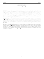
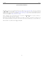
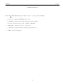
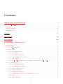
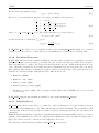
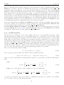
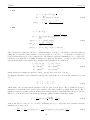
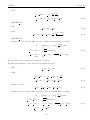
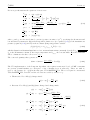
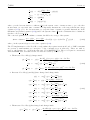
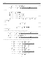
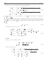
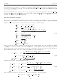
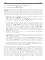
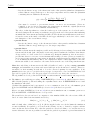
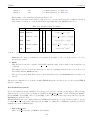
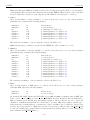
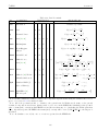
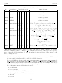
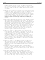
In practice the convergence of the Ewald sum is controlled by three variables: the real space cutoff rcut ;
the convergence parameter α and the largest reciprocal space vector k max used in the reciprocal space
sum. These are discussed more fully in Section 5.3.5. DL POLY 4 can provide estimates if requested (see
CONTROL file description 6.1.1).
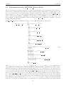
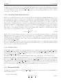
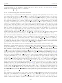
As its name implies the Smoothed Particle Mesh Ewald (SPME) method is a modification of the standard
Ewald method. DL POLY 4 implements the SPME method of Essmann et al. [66]. Formally, this method
is capable of treating van der Waals forces also, but in DL POLY 4 it is confined to electrostatic forces
only. The main difference from the standard Ewald method is in its treatment of the reciprocal space
terms. By means of an interpolation procedure involving (complex) B-splines, the sum in reciprocal space
is represented on a three dimensional rectangular grid. In this form the Fast Fourier Transform (FFT) may
be used to perform the primary mathematical operation, which is a 3D convolution. The efficiency of these
procedures greatly reduces the cost of the reciprocal space sum when the range of k vectors is large. The
method (briefly) is as follows (for full details see [66]):
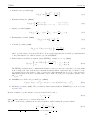
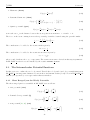
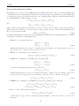
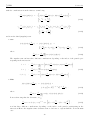
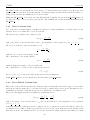
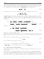
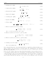
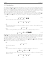
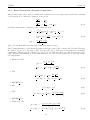
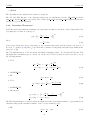
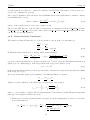
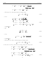
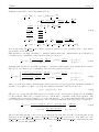
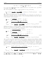
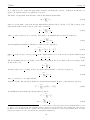
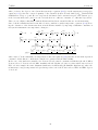
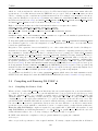
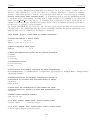
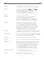
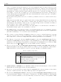
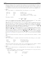
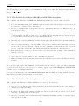
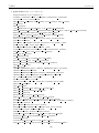
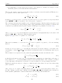
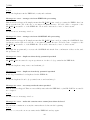
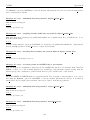
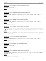
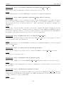
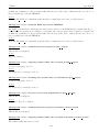
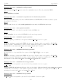
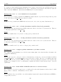
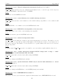
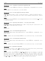
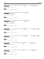
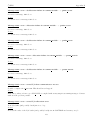
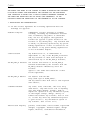
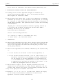
1. Interpolation of the exp(−i k · rj ) terms (given here for one dimension):
∞
∑
exp(2πi uj k/L) ≈ b(k)
Mn (uj − ℓ) exp(2πi kℓ/K) ,
(2.219)
ℓ=−∞
in which k is the integer index of the k vector in a principal direction, K is the total number of grid
points in the same direction and uj is the fractional coordinate of ion j scaled by a factor K (i.e.
uj = Ksxj ) . Note that the definition of the B-splines implies a dependence on the integer K, which
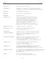
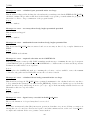
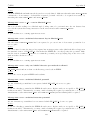
limits the formally infinite sum over ℓ. The coefficients Mn (u) are B-splines of order n and the factor
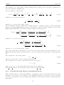
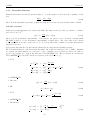
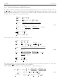
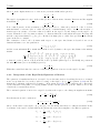
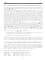
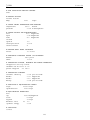
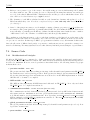
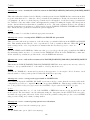
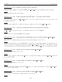
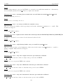
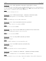
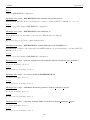
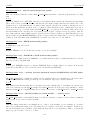
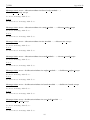
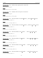
b(k) is a constant computable from the formula:
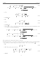
b(k) = exp(2πi (n − 1)k/K)
[n−2
∑
]−1
Mn (ℓ + 1) exp(2πi kℓ/K)
.
(2.220)
ℓ=0
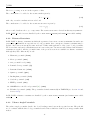
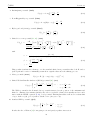
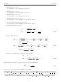
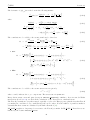
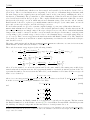
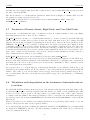
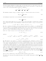
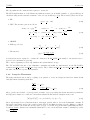
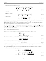
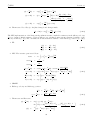
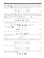
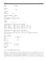
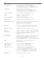
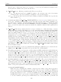
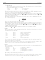
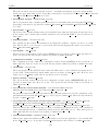
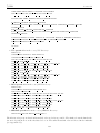
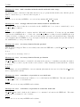
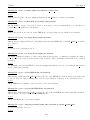
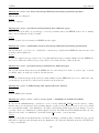
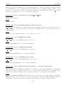
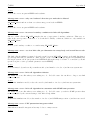
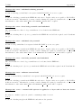
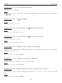
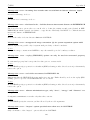
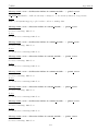
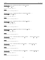
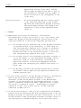
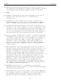
2. Approximation of the structure factor S(k):
S(k) ≈ b1 (k1 ) b2 (k2 ) b3 (k3 ) Q† (k1 , k2 , k3 ) ,
(2.221)
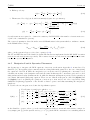
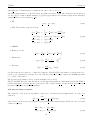
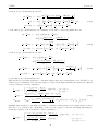
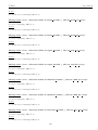
where Q† (k1 , k2 , k3 ) is the discrete Fourier transform of the charge array Q(ℓ1 , ℓ2 , ℓ3 ) defined as
Q(ℓ1 , ℓ2 , ℓ3 ) =
N
∑
j=1
qj
∑
Mn (u1j − ℓ1 − n1 L1 ) × Mn (u2j − ℓ2 − n2 L2 ) ×
n1 ,n2 ,n3
Mn (u3j − ℓ3 − n3 L3 ) ,
(2.222)
in which the sums over n1,2,3 etc are required to capture contributions from all relevant periodic cell
images (which in practice means the nearest images).
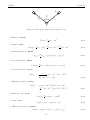
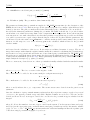
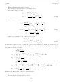
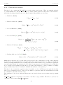
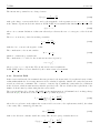
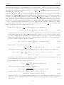
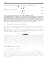
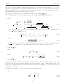
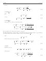
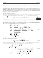
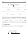
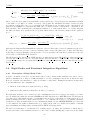
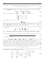
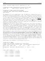
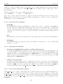
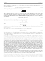
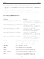
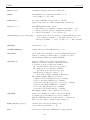
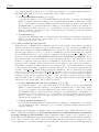
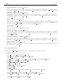
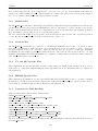
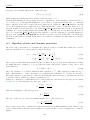
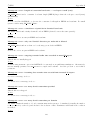
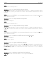
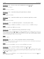
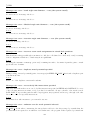
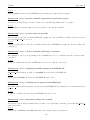
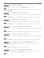
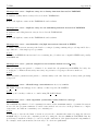
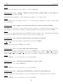
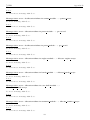
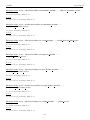
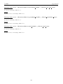
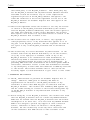
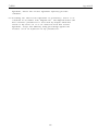
3. Approximating the reciprocal space energy Urecip :
Urecip =
∑
1
G† (k1 , k2 , k3 ) Q(k1 , k2 , k3 ) ,
2Vo ϵ0 ϵ k ,k ,k
1
where
G†
2
(2.223)
3
is the discrete Fourier transform of the function
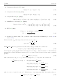
G(k1 , k2 , k3 ) =
exp(−k 2 /4α2 )
B(k1 , k2 , k3 ) (Q† (k1 , k2 , k3 ))∗ ,
k2
(2.224)
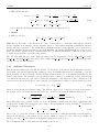
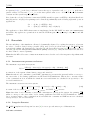
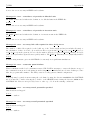
in which (Q† (k1 , k2 , k3 ))∗ is the complex conjugate of Q† (k1 , k2 , k3 ) and
B(k1 , k2 , k3 ) = |b1 (k1 )|2 |b2 (k2 )|2 |b3 (k3 )|2 .
(2.225)
The function G(k1 , k2 , k3 ) is thus a relatively simple product of the Gaussian screening term appearing in the conventional Ewald sum, the function B(k1 , k2 , k3 ) and the discrete Fourier transform of
Q(k1 , k2 , k3 ).
52