Download BayeScan v2.1 User Manual - Population Genetics CMPG Lab

BayeScan v2.1 User Manual
Matthieu Foll
January, 2012
1. Introduction
This program, BayeScan aims at identifying candidate loci under natural selection from genetic data,
using differences in allele frequencies between populations. BayeScan is based on the multinomialDirichlet model. One of the scenarios covered consists of an island model in which subpopulation
allele frequencies are correlated through a common migrant gene pool from which they differ in
varying degrees. The difference in allele frequency between this common gene pool and each
subpopulation is measured by a subpopulation specific FST coefficient. Therefore, this formulation
can consider realistic ecological scenarios where the effective size and the immigration rate may
differ among subpopulations.
Being Bayesian, BayeScan incorporates the uncertainty on allele frequencies due to small sample
sizes. In practice, very small sample size can be use, with the risk of a low power, but with no
particular risk of bias. Allele frequencies are estimated using different models depending on the type
of genetic marker used. In BayeScan, three different types of data can be used: (i) codominant data
(as SNPs or microsatellites), (ii) dominant binary data (as AFLPs) and (iii) AFLP band intensity, which
are neither considered as dominant nor codominant.
Selection is introduced by decomposing locus–population FST coefficients into a population-specific
component (beta), shared by all loci and a locus-specific component (alpha) shared by all the
populations using a logistic regression. Departure from neutrality at a given locus is assumed when
the locus-specific component is necessary to explain the observed pattern of diversity (alpha
significantly different from 0). A positive value of alpha suggests diversifying selection, whereas
negative values suggest balancing or purifying selection. This leads to two alternative models for
each locus, including or not the alpha component to model selection. BayeScan implements a
reversible-jump MCMC algorithm to estimate the posterior probability of each one of these models.
For each locus, BayeScan calculates a posterior probability for the model including selection. These
probabilities are very convenient to make decision in the context multiple testing (testing a large
number of markers simultaneously). Please note that a posterior probability can NOT be compared
directly to a p-value like the one obtained using the FDist software by Mark Beaumont. In Bayesian
statistics, model choice decision can be performed using the so-called “Bayes factors”. Given a
problem in which we have to choose between two models M1 and M2 (say neutral and selection),
on the basis of a data set N, the Bayes factor BF for model M2 is given by BF=P(N|M2)/P(N|M1). The
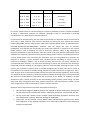
Bayes factor provides a scale of evidence in favor of one model versus another. For example, BF=2
indicates that the data favors model M2 over model M1 at odds of two to one. The next table gives
Jeffreys' scale of evidence for Bayes factors:
P(α≠0)
Bayes Factor (BF)
0.50 → 0.76
1 → 3
0.76 → 0.91
3 → 10
0.91 → 0.97
10 → 32
0.97 → 0.99
32 → 100
0.99 → 1.00
100 → ∞
log10(BF)
0 → 0.5
Jeffreys' interpretation
Barely worth mentioning
0.5 → 1
1 → 1.5
1.5 → 2
2 → ∞
Substantial
Strong
Very strong
Decisive
As a result, a Bayes factor of 3 corresponding to a posterior probability of 0.76, is already considered
as being a “substantial” evidence for selection (although p-value of 1-0.76=0.24 is generally
considered as a very weak signal in classical statistics).
In the context of multiple testing, we also need to incorporate our skepticism about the chance that
each locus is under selection. This is done in BayeScan by setting the prior odds for the neutral
model P(M1)/P(M2) and by using Posterior Odds (PO) instead of Bayes factors to make decisions:
PO=P(M2|N)/P(M1|N)=BF*P(M2)/P(M1). Posterior odds are simply the ratio of posterior
probabilities, and indicate how more likely the model with selection is compared to the neutral
model (Jeffrey’s scale of evidence can also be used with posterior odds). A big advantage of
posterior probabilities is that they directly allow the control of the False Discovery Rate (FDR). FDR is
defined as the expected proportion of false positives among outlier markers. Controlling for FDR has
a much greater power than controlling for familywise error rate using Bonferroni correction for
example. In practice, a given posterior odds threshold (chosen according to Jeffrey’s scale of
evidence for example), defines a set of outlier markers, and one can very easily calculate the
corresponding FDR. However, it is even more interesting to reverse the process by first choosing a
target FDR, and then looking for the highest posterior odds threshold achieving this FDR. In this
context, we can define a q-value, which is the FDR analogue of the p-value (note that a q-value is
only defined in the context of multiple testing, whereas a p-value is defined on a single test). The qvalue of given locus is the minimum FDR at which this locus may become significant. Since version
2.1, BayeScan directly calculates q-values for each locus and we encourage users to use (and report)
this measure to make decisions. Remember that in practice, if you choose, for example, a q-value
threshold of 10%, it means that 10% of the corresponding outlier markers (those having a q-value
lower than 10%) are expected to be false positives. Note that a 10% threshold for q-values is much
more stringent than a 10% threshold for p-values in classical statistics.
BayeScan and its improvements have been described successively in:



Foll, M and OE Gaggiotti (2008) A genome scan method to identify selected loci appropriate
for both dominant and codominant markers: A Bayesian perspective. Genetics 180: 977-993
Foll M, Fischer MC, Heckel G and L Excoffier (2010) Estimating population structure from
AFLP amplification intensity. Molecular Ecology 19: 4638-4647
Fischer MC, Foll M, Excoffier L and G Heckel (2011) Enhanced AFLP genome scans detect
local adaptation in high-altitude populations of a small rodent (Microtus arvalis). Molecular
Ecology 20: 1450–1462
2. BayeScan usage
BayeScan is command line based open source software, published under the GNU General Public
License as published by the Free Software Foundation (see http://www.gnu.org/licenses/). BayeScan
is coded using standard C++ and can be easily compiled under any system having a C++ compiler
available using the “Makefile” provided along with the source code (just typing “make” in a terminal
in the source folder should create the executable file). We provide executable ready to be used
under Windows, MacOS (intel), Linux 32bits and 64 bits. Since version 2.1, the command line version
of BayeScan has been optimized to work on multicore processors. In practice this means that it will
be much faster than previous versions as most machines now have at least 4 cores. By default
BayeScan will detect the number of cores available on your machine and use them all (this number is
written on the console at the beginning of the calculation). As this can make your computer difficult
to use for other tasks at the same time, you can also force BayeScan to use the number n you want
using the “-threads n” option.
We also provide a Graphical User Interface (GUI) version based on the exact same code as the
command line version, but only for Windows systems. This version does not support multicore
computing and will be much slower than the command line version on a multicore machine
(basically any recent machine).
The only compulsory argument to set in BayeScan is the input file describing the multilocus genetic
data (see input file preparation section for details about the file format). There is no limitation for
the size of the data, but your computer’s memory. All the other options have default values and can
to be set using the graphical user interface under Windows systems, or using command line
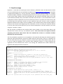
arguments for the command line version. Just starting the command line version without any
argument will display the full list of options:
--------------------------| Input
|
--------------------------alleles.txt Name of the genotypes data input file
-d discarded Optional input file containing list of loci to discard
-snp
Use SNP genotypes matrix
--------------------------| Output
|
---------------------------od .
Output file directory, default is the same as program file
-o alleles
Output file prefix, default is input file without the extension
-fstat
Only estimate F-stats (no selection)
-all_trace
Write out MCMC trace also for alpha paremeters (can be a very large
file)
--------------------------| Parameters of the chain |
---------------------------threads n
Number of threads used, default is number of cpu available
-n 5000
Number of outputted iterations, default is 5000
-thin 10
Thinning interval size, default is 10
-nbp 20
Number of pilot runs, default is 20
-pilot 5000 Length of pilot runs, default is 5000
-burn 50000 Burn-in length, default is 50000
--------------------------| Parameters of the model |
---------------------------pr_odds 10 Prior odds for the neutral model, default is 10
-lb_fis 0
Lower bound for uniform prior on Fis (dominant data), default is 0
-hb_fis 1
Higher bound for uniform prior on Fis (dominant data), default is 1
-beta_fis
Optional beta prior for Fis (dominant data, m_fis and sd_fis need to be
set)
-m_fis 0.05 Optional mean for beta prior on Fis (dominant data with -beta_fis)
-sd_fis 0.01 Optional std. deviation for beta prior on Fis (dominant data with
-beta_fis)
-aflp_pc 0.1 Threshold for the recessive genotype as a fraction of maximum band
intensity, default is 0.1
--------------------------| Output files
|
---------------------------out_pilot
Optional output file for pilot runs
-out_freq
Optional output file for allele frequencies
One possibility concerning the input file is to also provide a list of loci to discard from the calculation.
This can be convenient for example to remove monomorphic loci without having to manually delete
them. In BayeScan loci are indexed from 1 to the total number of loci. The list of loci to discard
should simply be a text file with the indexes of loci to discard, one on each line. Discarded loci don’t
take part in the calculation and no output is provided for them. The indexing of the other loci is
conserved in the output, allowing easy identification.
BayeScan automatically recognizes the type of data from the input file. The only exception is when
using a matrix of SNP genotypes, in which case one has to check the corresponding box in the GUI or
use the “-snp” argument in the command line version. This option has been used in Foll et al. (2010)
to compare the power of AFLPs and SNPs to estimate inbreeding coefficient FIS. If you are not
directly interested in FIS, you should rather use SNPs as a regular codominant data (see below),
which leads to much faster computation.
For the output files, one can choose the directory the files will be placed (default is the current
directory). As different files will be produces, one can also choose a common prefix for all the files. In
the command line version the default prefix is the name of the input file (without the file extension
if any). It is also possible to only estimate population specific F-statistics, as this was done in Foll et
al. (2010). Once BayeScan has successfully loaded your input file, a file called “yourprefix_Verif.txt”
is created and automatically opened in the GUI version using notepad. This file summarizes the
parameters you chose and the input data so you can check that everything has been correct
interpreted. In the GUI version, the estimated remaining time is indicated at the left of the bar.
BayeScan is using a Reversible Jump Markov Chain Monte Carlo (RJ-MCMC) algorithm to obtain
posterior distributions. This algorithm is stochastic and need time to attain convergence, and some
parameters can be adjusted. With large data it can be very time consuming (days of calculation). The
sample size corresponds to the number of iterations the program will write out and use for
estimation. The thinning interval is the number of iterations between two samples. This reduces the
autocorrelation of the data generated from a Markov chain. A burn-in period can be necessary to
attain convergence before starting the sampling. The total number of iterations is: sample size
multiplied by thinning interval, plus burn-in period. Proposal distributions have to be adjusted in
order to have acceptance rates between 0.25 and 0.45. These values are automatically tuned on the
basis of short successive pilot runs: by default we first run 5000 iterations, and then the proposals
are adjusted in order to reduce or increase acceptance rate for each parameter. We make by default
20 such pilot runs before starting the calculation. At the same time, we use those pilot runs to
choose the proposal distribution for the reversible jump. The best choice would be to take the full
conditional posterior distribution of alpha parameters. Because we don't know this distribution, we
use the pilot runs to have an estimation of the mean and variance for all alpha’s under the saturated
model (which contains all the alpha parameters). Then we use a normal proposal with these means
and variances, which is generally close to the full conditional distribution. The default values in
BayeScan for the MCMC algorithm parameters are quite conservative and ensure good convergence
in most cases. In particular, codominant or dominant binary data tends to attain convergence very
rapidly, and a long burn-in period may not be necessary. On the contrary, AFLPs using band intensity
data require long burn in period as well as many and long pilot runs. When calculation time is not a
problem, increasing the number of pilot runs would be the first thing to do. Increasing the sample
size is generally useless, and one should rather increase thinning interval.
As explained in the introduction, one needs to set the prior odds for the neutral model. When a
large amount of data is available (in particular a large number of populations and individuals), the
prior odds will have a low influence on the posterior odds. However, in the extreme case of totally
uninformative data, the posterior odds will simply be equal to the prior odds. This is for example the
case for uninformative loci such as monomorphic markers or markers with a very low minor allele
frequency. We advise people to exclude these markers from the analysis. Using a prior odds of 1
would mean that for every locus, one assume a priori that the model including selection is as likely
as the neutral model. This can lead to false positives when testing a large number of markers. For
example with uninformative data, one would conclude that half of the markers show a signal in
favour of selection. Higher prior odds will tend to eliminate false positives, but at the cost of
reducing the power to detect any marker under selection. A value of 10 seems reasonable for the
identification of candidate loci within a few hundreds of markers, whereas values up to 10 000 are
generally used in the context of genome wide association studies with millions of SNPs when people
want to identify only the top candidates.
Some parameters of the model can be adjusted specifically for AFLP markers as proposed by Foll and
Gaggiotti (2008) and Foll et al. (2010). Please refer to these articles for further details. In short, when
using AFLP markers as purely dominant binary data, BayeScan allows for deviation from HardyWeinberg equilibrium for the estimation of allele frequencies throw the introduction of inbreeding
coefficients FIS. However, it is not possible to estimate those coefficients from binary data, and we
therefore allow FIS to move freely within its prior range in order to still incorporate the uncertainty
on this parameter. When prior information is available on FIS (using for example some biological
knowledge about the species reproduction system, or some estimation based on another set of
codominant genetic markers), one should include it in BayeScan. By default BayeScan assume a
uniform prior between zero and one, which may be unrealistic for many species, as this leads to an
average FIS value of 0.5. In BayeScan there are two ways to define the prior for FIS: (i) using a uniform
prior, providing the two boundaries of the interval and (ii) using a beta prior, providing the mean and
variance of the distribution. Note that not all combination of mean and variance can be used with a
beta prior, and BayeScan will inform you if the values entered cannot be used.
Finally, you can tell the program to write out some optional additional files:

The allele frequencies estimated (posterior mean) for each marker in each population
when using dominant markers or AFLP amplification intensity data.



A file to check that the input files are read correctly and the parameters of the run.
Some information about the results of the pilot runs.
Some information about the acceptance rates for the different model parameters.
The last two files should generally be only useful for debugging if something goes wrong.
3. Input file preparation
BayeScan uses its own input file formats, which depend on the type of data used. All input files are
simply in text format, but note that UNICODE files are not recognized (be careful when exporting
from Excel).
-
Codominant markers:
When using codominant data, we advice people to use PGD spider, a software converter
developed by Heidi Lischer that can be freely downloaded from:
http://www.cmpg.unibe.ch/software/PGDSpider/
Example files for microsatellites and SNPs are given in the files respectively called
“test_msats.txt” and “test_SNPs.txt”. You have to indicate the number of loci and the
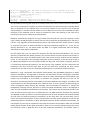
number of populations before the actual genetic data (see the examples). For each
population, there is one line per locus numbered from 1 to the number of loci. Each lines has
the same format as the following example:
“8 24
6
4 10
0
6
3
1”
“8” means that this is the 8th locus.
“24” is the total number of genes for this marker in this population (twice the number of
individuals for diploid data). It can be different for different markers to account for missing
data.
“6” is the number of alleles for the 8th locus. It has to be the same in all populations (even if
some alleles are not observed in some populations).
“4 10
0
6
3
1 ” are the number of observations for each of the 6 alleles in
this population for the 8th locus. These number must sum to the total number of genes in
the population, here 24.
-
Dominant binary markers:
For dominant binary AFLP markers an R script is provided to easily convert data from the
binary matrix format of AFLPDAT (Ehrich 2006 Molecular Ecology Notes 6: 603-604). The
input file format is quite similar to the codominant format, but the number of alleles does
not need to be set (as it is always assumed to be two) and one only need to indicate the
number of individuals having the band (“1”). An example is given in the file
“test_binary_AFLP.txt”. Each lines has the same format as the following example:
“35 30
13”
“35” means that this is the 35th locus.
“30” is the number of individuals for this marker in this population. It can be different for
different markers to account for missing data.
“13” is the number of individuals having the band (“1”).
-
Amplification intensity matrix for AFLP markers:
The format of this file is the same as the binary matrix format of AFLPDAT, but instead of
indicating 0 or 1 for each individual (in rows) at each locus (in columns), one needs to write
the corresponding measure of amplification intensity. The matrix of amplification intensity
can be obtained from software such as GeneMapper. An example is given in the file
“test_band_intensity_AFLP.txt”. At the beginning of each line, one has to indicate the index
of individuals starting from 1 and the index of population also starting from 1.
Using this type of data set in BayeScan requires very careful verification of your data as
explained in Foll et al. 2010. On average, amplification intensity should be twice for
dominant homozygotes compared to heterozygotes. This means that the difference in
amplification intensity due to different genotypes should be higher than the variance due to
noisy data. In practice, one should check that some marker exhibit a bimodal distribution for
non-zero amplification intensity. Additionally, one has to be sure that bimodality is not
caused by artefacts, like different plates, lab technician, day of analysis etc. One way to
check this is to look for X-linked markers where the two modes should correspond to the
two sexes. In order to help people dealing with this type of data, we provide some R
functions in the file “AFLP_data_functions.r”. The different functions are shortly described
below:

clean_intensity_matrix
We sometime observed some very high values of amplification intensity which can
correspond to sequencing errors. This function is looking for extreme values and
replaces them by missing data. Extreme values are defined as being three times
higher than the 95% quantile of the distribution. This definition can be changed.

convert_to_binary_bayescan
This function converts amplification intensity matrix to dominant binary data in
BayeScan format.

convert_to_binary_matrix
This function converts amplification intensity matrix to binary data in matrix format
(AFLPDAT format).

convert_from_binary_matrix
This function converts binary matrix to binary data in BayeScan format

pop_subset
This function allows to easily extract a subset of populations from a BayeScan band
intensity matrix input file.

discard_monomorphic
This function returns a list of monomorphic markers from an amplification intensity
matrix input file, ready to be used as a “discarded list” in BayeScan. For band
intensity data, the definition of “polymorphic” is more complicated, and you may
need this function.
More details about the functions can be found in the header of the file by opening it using a
text editor.
-
SNP genotype matrix:
This can be viewed as a special case of amplification intensity matrix where the genotype of
individuals is supposed to be known. It has exactly the same format but instead of intensity
values, on have to indicate for each individual at each locus the observed genotypes coded
as “0”, “1” and “2”. An example is provided in the file “test_genotype_SNP.txt”. Please note
that one has to check the corresponding box in the GUI or use the “-snp” argument in the
command line version to use this type of data. This option has been used in Foll et al. (2010)
to compare the power of AFLPs and SNPs to estimate inbreeding coefficient FIS. If you are
not directly interested in FIS, you should rather use SNPs as a regular codominant data (see
above), which leads to much faster computation.
4. Interpreting and plotting outputs
In this part we assumed that the prefix for the output has been set to “yourprefix”.
Most of the results you will need are in the “yourprefix_fst.txt” file created at the end of the
calculation. Each line of the file corresponds to one locus (eventually without the markers listed as
discarded in the input file), and contains the following values in this order:
-
-
The index of the locus corresponding to the index in the input file.
The posterior probability for the model including selection.
The logarithm of Posterior Odds to base 10 for the model including selection. Note that this
value is arbitrarily fixed to 1000 when the posterior probability is 1 (should be infinity).
The q-value for the model including selection.
The estimated alpha coefficient indicating the strength and direction of selection. A positive
value of alpha suggests diversifying selection, whereas negative values suggest balancing or
purifying selection.
The FST coefficient averaged over populations. In each population FST is calculated as the
posterior mean using model averaging.
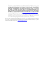
An R function is provided to plot and identify outlier using different criteria from this file. The
function is called “plot_bayescan” and is located in the “plot_R.r” file. The typical usage of the
function once loaded into R and being in the right directory is to type:
> plot_bayescan("yourprefix_fst.txt",FDR=0.05)
This will list the outliers having a q-value lower than 5% and produce a figure. More details about the
function can be found in the header of the file by opening it using a text editor.
The full output of the MCMC algorithm can be found in the file named “yourprefix.sel”. Each line
corresponds to an iteration in the MCMC algorithm and contains the following parameters in this
order (the first line contains the name of the columns):





The iteration index, starting after pilot runs and burn-in.
The logarithm of the likelihood
FIS coefficient for every population in the case of dominant or AFLP band intensity data
FST coefficient for every population
Alpha coefficients for every locus. Counting null value of alpha gives the posterior probability
for the neutral model. Since version 2.1, these coefficients are only written out if the option
“-all_trace“ is enabled.
Plotting posterior distributions and obtaining Highest Probability Density Interval (HPDI) for the
different parameters is very easy using R and from this file. First you have to load the file (be sure R
is looking in the right directory):
> mydata=read.table("yourprefix.sel",colClasses="numeric")
Then you can choose a parameter you are interested in, for example:
> parameter="Fst1"
Now this command will plot the posterior distribution for this parameter:
> plot(density(mydata[[parameter]]), xlab=parameter,
main=paste(parameter,"posterior distribution"))
If you have the “boa” package installed, this command will give you the 95% HPDI:
> boa.hpd(mydata[[parameter]],0.05)
The file “yourprefix_Verif.txt” helps to verify that the input file is read correctly.
Some optional output files can be produced depending on the data and option chosen:



The file “yourprefix_prop.txt” gives the results of the pilot runs.
The file “yourprefix_AccRte.txt” gives the evolution of the acceptance rate for the different
model parameters.
The file “yourprefix_freq.txt” contains the allele frequencies estimated (posterior mean) for
each marker in each population when using dominant markers or AFLP amplification
intensity data.
5. Contact
I would be very happy to help if you have some questions regarding BayeScan. However, before
writing me, please ask yourself the following questions:
-
-
-
-
Did I read completely the manual?
My input file is correctly formatted? Even if you used software to create it, try to open it
using a text editor. I personally recommend using Notepad++ (http://notepad-plusplus.org/) or TextPad (http://www.textpad.com/) under windows, which are free and very
powerful.
BayeScan is working as expected using the example input files provided? Compare your
input file with the example files provided. Try to oversimplify your input file to find the
problem (keep only one population and one locus for example).
If you are trying to use the console version, do you know the basic of commands? If not you
can read this 10 minutes tutorial for example:
http://wiki.vpslink.com/HOWTO:_Quick_Linux_Reference:_Learn_UNIX_in_10_minutes
If you have difficulties to use the R functions, do you know the basics of R? If not you can
read this introduction: http://cran.r-project.org/doc/manuals/R-intro.html.
If you are trying to compile BayeScan for a specific platform, do you have a C++ compiler
installed? If you don’t even know what this mean, you can ask any informatician around you,
even if he has no clue about population genetics… Also you will certainly have to remove the
“-static” option on the Makefile on line 4 to compile under MacOS.
-
-
If you are not sure whether BayeScan can be applied on your favorite species data set, I have
to admit I certainly won’t be able to know this better than you. The basic assumptions
behind BayeScan are summarized in the introduction of this manual, and you can find more
details in the related publications. Each violation of an assumption can lead to an excess of
false positive or eventually false negative, but this is generally difficult to predict. The
correct way to do is to make simulations mimicking your real data and to see what BayeScan
will produce. For example Fastsimcoal provides a very flexible way to simulate genetic data
over a wide range of demographic scenario (http://cmpg.unibe.ch/software/fastsimcoal/).
If you compare BayeScan with other methods aiming at identifying makers under selection
(FDist, detsel etc.) and find different results, that’s maybe not a bug, but a nice feature! We
are working hard to increase the power of our methods and to reduce false positives, so if
the new methods keep giving the same answers as previous ones, this is useless.
Of course there are certainly some hidden bugs in BayeScan, and I would be grateful if you identify
one of them… Despite the previous recommendations you should follow before contacting me, don’t
hesitate to send me a message here: [email protected] !