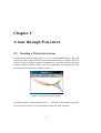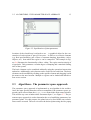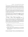
1
DLR Institute of Robotics and Mechatronics Robust Control PARADISE 2.0 PARAMETRIC ROBUSTNESS A NALYIS AND D ESIGN I NTERACTIVE S OFTWARE E NVIRONMENT U SER ’ S MANUAL PARADISE 2.0 U SER ’ S MANUAL How to Contact PARADISE: 8153-28-1847 Fax Robuste Regelung DLR Postfach 1116 82230 Wessling Mail http://www.op.dlr.de/FF-DR-RR/paradise Web [email protected] Technical support Product enhancement suggestions Bug reports Paradise User Manual c 1999, 2000 by DLR, Oberpfaffenhofen. The user should be aware that this product is protected by copyright law and international treaties. The authors and DLR shall under no circumstances be liable for any indirect, incidental or consequential damages caused by the provided software. Furthermore, the authors and DLR assure that the software tool and its documentation was developped with great care. However, the user should recognize that software and documentation still might contain errors and omissions for which the authors shall not be responsible. The software is not recommended to be used for applications in which errors or omissions could threaten life, injury or significant loss. All rights reserved. The software may be used or copied only under the terms of the license agreement. Please note, that most of the referred soft- and hardware names in this document are registered trademarks and are subject to legal requirements. Printing History: Date Version Author 2000 2.0 M. Muhler 1997-1999 1.0 D. Odenthal Preface Thank you for you interest in PARADISE, a new toolbox for robust parametric control. Robust parametric control has a long tradition, with roots back to [Vys86] design rules for governors for stable speed control of engines and the Boundary Crossing Theorem by [FD29] in 1929, which was motivated by aircraft flutter analysis. However, up to now robust parametric control was rarely applied in the practically oriented field of industrial control. The main reason lies simply in the fact that no software was available for this type of problems. As you already can tell from the name, a parametric plant model is required as basis of robust parametric control algorithms. Handling and manipulating such kind of models is not at all a trivial task. It requires symbolic computer programs like e.g. Maple or Mathematica to facilitate the application of robust control algorithms. But even with such modern programs it still requires deeper insight into the methods to solve robust control problems. PARADISE not only keeps you away from lengthy and annoying symbolic calculations. It offers you easy-to-use graphical user interfaces to use algorithms. Simply read in a Simulink model and let PAR ADISE compute the symbolic closed loop model for you. Then, do your closedloop specifications graphically, use an adequate design method and graphically visualize the solution. Chapter 1 gives you a short introduction to the basis of robust control. Users with some knowledge of robust control may want to skip this chapter. Chapter 2 takes you on a short trip through PARADISE to give you an impression about the possibilities of this toolbox. Chapter 3 explains how to input your plant and controller structure and your problem specifications. The remaining chapters explain the robust control algorithms in more detail and demonstrate, how you can solve these problems using PARADISE. Of course a complete introduction to robust parametric control goes beyond the scope of this manual. For a deeper insight the reader ˇ is refered to the literature, for example [ABK 93a, S69]. Contents 1 Introduction to robust control 1 1.1 Parametric models and uncertainty . . . . . . . . . . . . . . . . . 1 1.2 Multi-model representation . . . . . . . . . . . . . . . . . . . . . 3 1.3 Performance specifications . . . . . . . . . . . . . . . . . . . . . 4 1.4 Robust controller design and analysis . . . . . . . . . . . . . . . 6 2 A tour through PARADISE 9 2.1 Starting a PARADISE session . . . . . . . . . . . . . . . . . . . . 2.2 Input specifications . . . . . . . . . . . . . . . . . . . . . . . . . 10 2.3 9 2.2.1 The plant . . . . . . . . . . . . . . . . . . . . . . . . . . 10 2.2.2 The operating domain . . . . . . . . . . . . . . . . . . . 12 2.2.3 The -region . . . . . . . . . . . . . . . . . . . . . . . . 12 Algorithms - The parameter space approach . . . . . . . . . . . . 13 3 Getting started with PARADISE 17 3.1 Starting and quitting a PARADISE session . . . . . . . . . . . . . 17 3.2 Plant specification . . . . . . . . . . . . . . . . . . . . . . . . . . 20 3.2.1 Using Simulink . . . . . . . . . . . . . . . . . . . . . . . 20 3.2.2 Simulink is not available . . . . . . . . . . . . . . . . . . 22 3.2.3 Multi model specification . . . . . . . . . . . . . . . . . 23 3.3 Parameter specification . . . . . . . . . . . . . . . . . . . . . . . 25 3.4 The -region editor . . . . . . . . . . . . . . . . . . . . . . . . . 28 vii CONTENTS viii 4 The parameter space method 33 4.1 Some introducing theory . . . . . . . . . . . . . . . . . . . . . . 33 4.2 The parameter plane menu . . . . . . . . . . . . . . . . . . . . . 37 4.3 Design examples for the parameter space method . . . . . . . . . 40 4.3.1 Design example 1: Crane . . . . . . . . . . . . . . . . . . 40 4.3.2 Design example 2: F4E fighter aircraft . . . . . . . . . . . 45 5 Design in an invariance plane 49 5.1 Introduction . . . . . . . . . . . . . . . . . . . . . . . . . . . . . 49 5.2 Theoretical background . . . . . . . . . . . . . . . . . . . . . . . 49 5.2.1 Design in an Invariance Plane . . . . . . . . . . . . . . . 50 Example : Crane . . . . . . . . . . . . . . . . . . . . . . . . . . 51 5.3 Bibliography 61 Chapter 1 Introduction to robust control Almost all technical systems depend on varying or uncertain parameters. Just consider the velocity or mass of vehicles, the oil temperature of hydraulic systems, or the rope length and load mass of the crane illustrated in Figure 1.1. These parameters may vary more or less significantly within certain bounds and they influence the system dynamics. Traditional control design approaches, however, consider a fixed operating point in the hope that the resulting controller is robust enough to stabilize the plant for different operating conditions. These approaches definitely yield good results if the parameter variations are small or the system dynamics is not too sensitive with respect to these parameters. For significant parameter variations these control design methods reach their performance limits. New design approaches, which already incorporate the plant uncertainty in the design step are then required. 1.1 Parametric models and uncertainty Robust parametric control offers several design approaches for this type of problems. The basis of these approaches is a parametric model. As an example consider the crane in Figure 1.1. The task of the operator of such a crane is to pick up a load and transport it to another location while preventing the load from swaying. Especially, when placing a load precisely for example on top of a truck or on a container ship, the load should have stopped completely from swaying, which requires training and full attention of the operator. An anti-sway control system certainly will support the operator and help him to operate the loads faster. The design of such a control system has to handle the uncertainty in the rope length and the load mass and guarantee stability 1 CHAPTER 1. INTRODUCTION TO ROBUST CONTROL 2 Figure 1.1: A crane and its schematic representation for all possible operating conditions. The load mass may vary from the hook up to the maximal load mass and also the rope length varies within mass known limits, other crane parameters like the crab mass are assumed tot be known. The resulting rectangular operating domain designated as is illustrated in Figure 1.2. Figure 1.2: Rectangular operating domain of the crane The design of a control system requires in the first step a model of the plant. A 1.2. MULTI-MODEL REPRESENTATION 3 linear state space representation of the plant dynamics is # # $ # # $ # # # # &% "! # # $ ( # , (1.1) $ # # ' )(* # ' + % + where the states are crab position -/. , crab velocity -10 , rope angle -12 , and rope angle rate -13 . A stability analysis of the crane can be performed using its characteristic polynomial. It is 465879 9 9 ;: !=<?>A@ 5B7DC 'FE : ! 7 0 5B7 0 ( 5 $ * ( +GHI: % GHJ: (1.2) The plant parameters enter into the characteristic polynomial and, hence, make the plant dynamics depending on these parameters. For this simple example the roots of the polynomial can be calculated explicitly. They are 7 .LK 0 ! # 7 2HK 3 ! MON 5 $ * ( PGH;: % GH (1.3) It is a fourth order system with a double pole at the origin and a complex conjugate pole pair varying with the operating parameters along the imaginary axis from to . For details about parametric modeling the reader is referred to the literature, for example [Cel91]. 5 $ ( GH/: GH % 1.2 5 $ ( HG ;: GH % Multi-model representation Not in all cases symbolic system equations can be retrieved, for instance, if the plant is highly nonlinear and complex. In those cases it is often possible to obtain a finite set of local linear models for a number of distinct operating points, for example by means of system identification of the open-loop plant or by linearization of a nonlinear plant model. These plant representatives can be used for the controller design. A typical application is flight control. Especially, modern high performance fighter aircrafts are aerodynamically unstable and need to be controlled. Figure 1.3 shows a sketch of such a plane equipped with additional canards to increase maneuverability. The task here is to control the short period mode which is described by the 4 CHAPTER 1. INTRODUCTION TO ROBUST CONTROL Figure 1.3: Sketch of a fighter aircraft QSR V 0.W.. V# T states normal acceleration and pitch rate . The linearized state equations are ^. . X 0 X . 2 S Q R # , "!U V 0W0 V W0 2 (1.4) []T \ ( $HZ #V 'YV H$ Z [_\ where the elevator actuator state with a time constant of 1/14 is considered. The operating domain of the aeroplane – the so-called flight envelope illustrated in Figure 1.4 – describes the admissible range of altitude in dependency of the Mach number. Nominal values for the system description (1.4) are given in Table 1.1 for the four representative flight conditions indicated in Figure 1.4. 1.3 Performance specifications Back to the crane example. To stabilize this plant it would suffice to shift the poles only a little bit into the left complex halfplane. In view of a practical realization this is certainly not sufficient since the damping still could be arbitrarily small. Here comes in the notion of -stability to assure sufficient stability margins. Considering the operating domain in Figure 1.2 it cannot be the aim of the design to specify precisely the location of the poles in dependency of the operating point. The design goal is reached if the damping is sufficiently large. This is the case if 1.3. PERFORMANCE SPECIFICATIONS 5 Figure 1.4: Flight envelope the roots of the closed-loop system for all possible operating points have a degree of damping larger then a value . Furthermore, a maximal settling time might be required. This corresponds to a maximal real part of the roots not larger than a certain value . Both conditions can be visualized graphically in the complex -plane, see Figure 1.5 a), b). `?a bca 7 hji fJg d8e ke hli fJg me hli fg ne hli fJg Figure 1.5: Examples for -regions: A line parallel to the imaginary axis guarantees a maximal settling time (a), a pair of lines a minimal degree of damping(b), a circle limits the bandwidth (c). All these conditions can be satisfied simultaneously by the intersecting region (d). The admissible region for closed-loop eigenvalues is denoted as , a system is called -stable if all its eigenvalues are located in this region and an uncertain system is called robustly -stable if all eigenvalues for all operating conditions are contained in . The definition of -stability permits arbitrary regions in the complex -plane and does not underlie any restrictions. It also includes the special cases of the left halfplane for Hurwitz stability and the unit circle for Schur stability. o 7 o CHAPTER 1. INTRODUCTION TO ROBUST CONTROL 6 Mach Altitude [ft] p .W. p .X0 p .X2 p 0. p 0W0 p 0W2 . . 0 FC 1 0.5 5000 qsrtvuwux yztv~y uxtvy} rtv{x~w qsrtvw}y{ qsyytvu qsuztvzw qsytv{tvr z FC 2 0.85 5000 qsytvzr{ }rtvz{ {xtv} rtv{{ry qsytv~yw qsytvuu qs{z{tv{ qsy~tvztvuw r FC 3 0.9 35000 FC 4 1.5 35000 q|rtvxxz qsrtv}yx{ ywtvyy {xtvux w~tv~ yzwtvu rtvrw{ry qsrtvxwux qsrtvx}wz q|ytv{{} q|yrtvwy q|rtvw q|w}tvru q|yz}tvx qsrytv}tvwx z q|rtvwz W~tv 5B7 ' W. ._: 587 ' 0W0: ' .X0 0. ! # V V V V The region is specified by its boundary . Besides lines, adequate elements to describe the boundary of a -region are circles, hyperbolas, and ellipses. Lines 7. 70 Table 1.1: Model data for an F4-E aircraft for four typical flight conditions. The eigenvalues and result from parallel to the imaginary axis restrict the settling time, circles the bandwidth. Circles can be used to limit the bandwidth, or – in its inverted version – to guarantee a minimal bandwidth. In order to fulfil several specifications simultaneously the intersection of basic elements can be formed, see Figure 1.5d). The -region is not necessarily simply connected. Just imagine a plant with a pole pair close to the origin, whose effect on the system dynamics is almost cancelled by a close pair of zeros. It would not be wise to move this pole pair to the left such that it satisfies a certain degree of damping. A better approach is to -stabilize only the remaining poles, while the pole pair remains more at its open-loop location. A pair of circles with small radius around the poles forming a union with the remaining -region guarantees that the poles do not move too far away from the zeros. 1.4 Robust controller design and analysis Back to the crane design example. The task is to determine a controller which robustly -stabilizes the crane for the entire operating domain. In this example state feedback will be investigated. , ! ' 1.4. ROBUST CONTROLLER DESIGN AND ANALYSIS 7 . In case of a step input the initial force is proportional to the controller gain . It can be adjusted according to the efficiency of the used actuator, for the design example it will be set to 500. The gain feeds back the rope angle rate which is difficult to measure. Since the rope angle rate is observable from the rope angle, its measurement can be neglected which leads to . Nothing can be said at this moment about and . 3 0 2 3 ! # With these simple considerations it was possible to reduce the number of undetermined controller parameters and, hence, simplify the design. The closed loop characteristic polynomial is now with m/s and kg ! H$ # 0 ! H$ ##c# 46587J9 9 9 0 9 2: ! 58 ##c# ( $H# % 0 7 ( 5 $H#c#c## ( #c# O( $# ' 2: 7 0 ( (0] 7 2 ( $H##c# 7 3 :G 5 $H#c## J: The design step has to assure that for the resulting nominal values of 0 and 2 the roots of the characteristic polynomial lie in the region for all possible operating conditions. In general, this cannot be accomplished in one design step for the entire operating domain. A more practically oriented way of robust control design is simultaneous -stabilization which is as follows: Step 1: Select a finite number of nominal operating points which adequately represent the operating domain. In case of a symbolic model description chose a number of operating points and calculate the nominal system equations. A good choice are the vertices of the operating domain, see Figure 1.2. In case of a multi-model description these nominal system descriptions are already given. Step 2: Determine a controller which simultaneously -stabilizes the representatives of Step 1. Despite of this simplification the design step still remains a complicated task. The parameter space approach which you will get to know in Chapter 4 yields as its result the entire set of controller parameters for which a nominal operating point is -stable. Computing this set for each representative and forming the intersection of all sets results in the set of all controller parameters which simultaneously -stabilize the representatives. To complete this step select an adequate solution from the set. .W = 5 E 0 9 0: = 0 This procedure is illustrated in Figure 1.6. For a given region the set of -stabilizing controller parameters and are calculated for the two and . The intersection representatives of both sets simultaneously stabilizes the two representatives. 5 E . 9 _. : ! = .W = 0 Step 3: Since the controller was designed only to simultaneously -stabilize the representatives it has to undergo a precise analysis which has to verify CHAPTER 1. INTRODUCTION TO ROBUST CONTROL 8 Figure 1.6: Simultaneous -stabilization of representatives that the controller is robustly -stable for the entire operating domain. If this test passes, the design is finished. Otherwise, go back to Step 1 and add more representatives, especially from the regions where the analysis indicated -instability. The controller structure assumed for the design step is crucial for its success. High degree controllers may give more freedom in the design directions, however, within an interactive design procedure the design engineer easily may loose survey of the influence of each controller parameter on the system dynamics. For this reason it is recommended to start with the most simple controller structure. If a design fails, relax the design specifications and try again. If this design succeeds, investigate how to augment the controller structure to meet more restrictive specifications. As you can already tell from this “recipe” robust control design is mostly not a straight forward design procedure. It is much more a learning process of the design engineer supported by robust control methods. In this learning process the engineer will get much more insight into the plant dynamics and its dependency on the uncertain and controller parameters. This “engineering art” approach is justified by the resulting controller which exploits the highest possible potential due to the parametric basis of the design and the mapping of “sharp” boundaries, i.e. whenever a boundary in parameter space is crossed, then also an eigenvalue crosses the boundary of the chosen -stability region. 1 Chapter 2 A tour through PARADISE 2.1 Starting a PARADISE session To start up the toolbox simply type paradise at the Matlab-prompt. This will start up the main control window and automatically load the symbolic libraries, which are used to perform symbolic computations. From the menus of the main control window all further inputs can be accomplished and in general the user does not have to return to the Matlab window. Figure 2.1: PARADISE main window The main window is illustrated in Figure 2.1. The logo of the toolbox represents the color-coded value set of a track guided vehicle for fixed frequency. 9 CHAPTER 2. A TOUR THROUGH PARADISE 10 2.2 Input specifications 2.2.1 The plant Different kinds of inputs are necessary. The most obvious one is the plant itself. For this purpose a graphical user interface (GUI) was developed. PARADISE offers two different ways to specify the plant and controller structure: The more comfortable manner is the plant specification via Simulink. Once the user has selected the desired model, the information contained in the Simulink model is passed to the symbolic computation part, where a parametric representation of the closed-loop is calculated. If the Simulink model is changed the system equations have to be re-calculated. In order to save computation time, especially for larger systems, the symbolic system equations can be saved. When re-reading the Simulink-model in a later session, the saved data will be passed to the symbolic computation part without re-calculating the system equations from the Simulink model. If Simulink is not available, the closed-loop system equations (state-space or transfer function representation) have to be typed in manually. Figure 2.2 shows an example of a Simulink model. It illustrates the block diagram of a crane positioning control. The example represents a continuous plant family. PARADISE also allows to handle multi-model representations, where a finite number of linear plants are given as representatives of a nonlinear plant. Typical applications are flight control problems where only linearized models for various flight conditions are given. Figure 2.2: Simulink model of the crane 2.2. INPUT SPECIFICATIONS 11 The description of the block Crane in the Simulink model points to another feature of PARADISE, see Figure 2.3. Figure 2.3: Parametric representation of plants This block contains the description of the crane dynamics which is of fourth order for the linearized crane model as it is used here. The state space matrices were given in a very general form, for example 58999 ` : ! # $ # # # # # # # # 0V # W2 # $ 3V W2 # The entries of this matrix depend on crane parameters like crab mass, load mass, and rope length. This dependency could, of course, be declared in the Simulink model. However, if the system order is large, the detailed specification of the matrices in the Simulink block would be quite awkward and could easily lead to typing errors. To facilitate this procedure, it is possible to substitute Simulink parameters after the symbolic system equations are determined: the parameters contained in the Simulink model are determined from the symbolic equations, see Figure 2.4. The user now has the possibility to substitute these parameters by their actual dependency. In the example, was replaced by . Of course not all parameters have to be replaced, like for example the controller parameters to . 3 V 0W2 £ &¢¡ % . CHAPTER 2. A TOUR THROUGH PARADISE 12 Figure 2.4: Substitution of Simulink parameters 2.2.2 The operating domain After a substitution was performed the resulting parameters have to be classified. Three classes of parameters exist: ¤ ¤ Varying parameters: These are plant parameters which are uncertain (for example the crab mass) or vary but can be measured. ¤ Fixed parameters: These are plant parameters which will not change their value (for example the wheel base of a car) Controller parameters to be determined by the design process The uncertain parameters are assumed to vary within given intervals. The interface in Figure 2.5 allows the specification of these values. Also, the values for fixed and controller parameters have to be set. 2.2.3 The ¥ -region For technical applications Hurwitz-stability is mostly not sufficient. Further specifications, like settling time, damping, and bandwidth, have to be met. Several specifications can be translated into locations of eigenvalues which leads to a restricted set of eigenvalues in the left half plane. This set of admissible eigenvalue 2.3. ALGORITHMS - THE PARAMETER SPACE APPROACH 13 Figure 2.5: Specification of plant parameters locations of the closed-loop is referred to as . A graphical editor for the construction of such regions is part of PARADISE. It offers a set of basic elements (e.g. Real part limitation, pair of lines of constant damping, hyperbolas, circles, ellipses, etc.) from which the region can be composed. The example in Figure 2.6 illustrates the functionality of the -editor. The region consists simply of a hyperbola. This guarantees a certain degree of damping and a maximal settling time of the system. The basic elements can be combined arbitrarily using the operations intersection and union. Additionally, each element can be used in its inverted form. The basic elements can be modified by clicking on the specific element and dragging it with the mouse to the new location. Multiple -regions can be loaded and edited in a PARADISE session. 2.3 Algorithms - The parameter space approach The parameter space approach is implemented as an algorithm in the toolbox. Once the input specifications have been accomplished, the parameter space approach can be selected from the Algorithms-menu in the main control window. This will fire up a new window titled “Parameter Space”, see Figure 2.7. The parameter space approach is used to determine the set of stabilizing parameters in a parameter plane. For this purpose, the plane has to be fixed before any calculations can be executed. The user can select the desired plane using the two popup CHAPTER 2. A TOUR THROUGH PARADISE 14 Figure 2.6: -region editor menues displayed in Figure 2.7. After the plane was specified the user starts the computations of the stability boundaries from the Run-menu. An example is illustrated in Figure 2.7. Dashed lines identify “real root” boundaries, solid lines “complex root” (see section 4.1) boundaries. The stability boundaries divide the parameter plane into a finite number of regions. By checking -stability of each region in the parameter plane the set of simultaneously -stabilizing parameters can be identified. This is accomplished by selecting the appropriate function from the Options-menu and selecting different points in the parameter plane by mouse click. The checked point is colored green, if this pont is -stable. A red colored star indicates instability. Several others functionalities are implemented, for example scaling and identification of curves. 2.3. ALGORITHMS - THE PARAMETER SPACE APPROACH Figure 2.7: Parameter space 15 16 CHAPTER 2. A TOUR THROUGH PARADISE Chapter 3 Getting started with PARADISE This chapter explains in detail how to input a plant and design specifications in PARADISE. It assumes that the toolbox is installed correctly. For information on installation please see the file INSTALL. 3.1 Starting and quitting a PARADISE session Simply start a Matlab session and type paradise at the Matlab prompt. The message loading libraries... will appear, completed by done when the initialization of the Extended symbolic toolbox finishes. At the same time the PARADISE main window appears. From there other graphical user interfaces can be launched which are necessary for input specifications and starting algorithms. PARADISE can be shut down on different ways: ¤ ¤ PARADISE automatically quits when shutting down the Matlab session. ¤ ¦ Select “File Exit” from the PARADISE main window. This will only shut down PARADISE, not your Matlab session. Type paradise(’quit’) or paradise(’bye’) at the Matlab prompt. In all cases you will be asked to save modified plants. 17 CHAPTER 3. GETTING STARTED WITH PARADISE 18 Main window menus File: Save current model data: This saves the data of the currently active model. The name of this model is displayed in the title menu of the PARADISE main window. The following information will be stored: Symbolic system representation and parameter substitutions (see below) in a file named systemname.ssr. Parameter settings (e.g. upper and lower bounds of uncertain parameters, nominal values of representatives, controller and fixed parameters) and description of the -regions are stored in a file named systemname.dat Save all model data: All models currently open will be saved. Remove current model: The currently active model will be removed from the PARADISE session. If necessary the user will be asked to save the model data. Remove all models: This item removes all opened models from the running session. If necessary the user will be asked to save the model data. Save system to workspace: The system equations of the currently activated model are saved to the Matlab workspace for center of q-box: for vertices of q-box: for representatives: as LTI-objects systemname C, systemname V i or systemname R i corresponding to the number of vertices or representatives respectively. Note, that this item as well as the next requires the control system toolbox! Save system to file: This item opens the file selection box and saves the system equations of the currently activated model for center of q-box: 3.1. STARTING AND QUITTING A PARADISE SESSION 19 for vertices of q-box: for representatives: as LTI-objects systemname C, systemname V i or systemname R i respectively to the selected file. Exit PARADISE: Quits the PARADISE session. Input: Plant specification: Load new model: This opens a file selection box from where the desired model can be selected. Reload model: The symbolic closed loop equations will be regenerated, for example if the associated Simulink model has been changed by the user. Gamma editor: Starts the -region editor. Parameter specification: Opens a GUI where all parameter settings for the active plant can be specified. Algorithms: Parameter space: This command opens a window for computation of stability boundaries in parameter space ?: Help: Opens the help window (to be done). About Paradise: System name: This is a dynamic menu item listing the names of currently opened models. If only one model is opened its name will be listed but cannot be activated. If 20 CHAPTER 3. GETTING STARTED WITH PARADISE more than one system is loaded the menu item changes to a pulldown menu from where the current model can be selected. (Note that due to a Matlab bug the wrong system name is displayed. To find about the currently active system open the pulldown menu. The active system is marked.) Algorithms usually apply to the currently active model. Parameter settings will be updated in the corresponding windows if the active model is being changed. 3.2 Plant specification 3.2.1 Using Simulink The most comfortable way to specify a plant is to use Simulink. PARADISE reads in the specified plant and computes the closed-loop equations of the model via the Extended Symbolic Toolbox. Simply specify the plant in its parametric representation. As an example consider the crane example introduced in Chapter 1. The simulink model is shown in Figure 2.2. The state space block contains the plant description of the crane with its parameters in algebraic form. The Simulink model has to be created in advance and stored in a file. To read it in Plant specification”. This opens within PARADISE select “Input a file selection box from where you can select the desired model. ¦ When the model is loaded for the first time, the symbolic computation of the closed loop equations will be started automatically. You are informed about this action by the message Connecting system....... When finished, the required computation time will be displayed. For larger systems this step may be quite time consuming. Therefore, the symbolic closed loop equations can be saved to a file when selecting “File Save current model data”. The resulting file will be named systemname.ssr. It is an ASCII file, for the crane its contents is: ¦ _a := [[[0, 1, 0, 0], [-(b2*k1), -(b2*k2), a23 - b2*k3, -(b2*k4)], [0, 0, 0, 1], [-(b4*k1), -(b4*k2), a43 - b4*k3, -(b4*k4)]]]; _b := [[[0], [b2], [0], [b4]]]; _c := [[[1, 0, 0, 0], [0, 1, 0, 0], [0, 0, 1, 0], [0, 0, 0, 1]]]; _d := [[[0], [0], [0], [0]]]; _num := Cranenum; _den := Craneden; _cp := [-(a43*b2*k1) + a23*b4*k1 - a43*b2*k2*_s + a23*b4*k2*_s a43*_sˆ2 + b2*k1*_sˆ2 + b4*k3*_sˆ2 + b2*k2*_sˆ3 + b4*k4*_sˆ3 + _sˆ4]; 3.2. PLANT SPECIFICATION 21 _sub := [[a23, a43, b2, b4, k1, k2, k3, k4], [(g*mL)/mC, -((g*(mC + mL))/(l*mC)), mCˆ(-1), -(1/(l*mC)), k1, k2, k3, k4], [g, mC, mL, l], [g, mC, mL, l]]; To avoid naming conflicts the internal variables start with . When launching a new PARADISE session with this model the computation of the closed loop equations will be skipped if the file systemname.ssr is found. Instead, the information contained in this file will be read in by the Extended Symbolic Toolbox and is available in the session. When the Simulink model is modified the closed loop equations are inconsistent with the current model and have to be regenerated. This can be performed selecting “Input Plant specification Reload current model”. ¦ ¦ Note: The model cannot be used for numeric simulation in Simulink as long as no specific values for the plant parameters are given. However, you can be treat this model with PARADISE which computes the parametric closed-loop model via the Extended Symbolic Toolbox. If you want to simulate the model you have to specify the plant parameters at the Matlab prompt, for example mL=500; mC=1000; .... Also note that this does not affect the parametric model, i.e. though a numeric value is defined for example for in the Matlab workspace, will still be treated as a symbol within PARADISE. The following list of blocks is currently supported by PARADISE: Transfer Function State Space Zero Pole Integrator Gain Multiplexer (Mux) Demultiplexer (Demux) Summation (Sum) Selector all Source blocks, e.g. Step all Sink Blocks, e.g. Display, Scope PID Controller Matrix Gain Model Info You can use Matlab matrix creation functions, e.g. eye(2), or ones(2,3). Please do not use any submodels. CHAPTER 3. GETTING STARTED WITH PARADISE 22 3.2.2 Simulink is not available Of course you can use PARADISE without Simulink. In this case the input procedure is not as comfortable but offers more flexibility if you are familiar with Maple. The steps are as follows: 1. Open your favorite text editor and create a file which has the same format as the one illustrated on page 20. You only have to specify either the system matrices or the corresponding transfer function, e.g. the two files _a := [[[0, 1, 0, 0], [-(b2*k1), -(b2*k2), a23 - b2*k3, -(b2*k4)], [0, 0, 0, 1], [-(b4*k1), -(b4*k2), a43 - b4*k3, -(b4*k4)]]]; _b := [[[0], [b2], [0], [b4]]]; _c := [[[1, 0, 0, 0], [0, 1, 0, 0], [0, 0, 1, 0], [0, 0, 0, 1]]]; _d := [[[0], [0], [0], [0]]]; and _num := [1]; _den := [-(a43*b2*k1) + a23*b4*k1 - a43*b2*k2*_s + a23*b4*k2*_s - a43*_sˆ2 + b2*k1*_sˆ2 + b4*k3*_sˆ2 + b2*k2*_sˆ3 + b4*k4*_sˆ3 + _sˆ4]; represent the same system, where in the latter case numerator and denominator of the transfer function have been given. The characteristic polynomial does not have to be specified, it will be calculated automatically. Also the parameter substitutions can be performed later within the corresponding user interface, however, you are free to specify it already in the text file as shown in the example on page 20. From the samples it should be easy to tell the required syntax. Experts: The file is interpreted by the Extended Symbolic Toolbox, i.e. it is of pure Maple syntax. You do not need to specify the state space representation explicitly. It can be the result of arbitrary symbolic calculations, where at the end the system matrices a, b, c, d or num and den, respectively, result. 2. Save the file to disk using the extension ssr. 3.2. PLANT SPECIFICATION 23 ¦ ¦ 3. Select the command “Input Plant specification Load new model”. This opens a file selection box from where you chose the file just specified. Note for Simulink users: Chosing the file systemname.mdl automatically starts Simulink. If you want to omit this and the symbolic closed loop equations are already saved (i.e. systemname.ssr exists) you can of course use the ssr-file. This feature is especially useful when only a limited number of Simulink licenses is available in a computer network and you only want to read in a model. In some cases the symbolic representation of the plant may be quite lengthy which can really make the plant specification in a Simulink state space box pretty annoying. For this case the symbolic description of the state space model can be specified in a file. This is convenient especially in those cases where the state space model is the result of a Maple session and already available in the desired format. The state space model has to be stored in advance to a file named systemname.sym as shown in the following sample: ASymb := [[0, 1, 0, 0], [0, 0, a23, 0], [0, 0, 0, 1], [0, 0, a43, 0]]; BSymb := [[0], [b2], [0], [b4]]; CSymb := convert(array(1..4,1..4,identity),listlist); DSymb := [[0], [0], [0], [0]]; In this example the Maple commands array and listlist were used instead of [[1, 0, 0, 0], ..., [0, 0, 0, 1]] for the output matrix. The Simulink state space box has to be filled then with the substitutes ASymb, BSymb, CSymb, and DSymb. Note that the representation may be mixed, e.g. only a substitute for the input matrix is used while the other matrices are specified conventionally in the Simulink state space box. 3.2.3 Multi model specification The multi model approach pointed out in Chapter 1 requires a special format for the plant input. Consider the case that a plant is not represented by a contin, uous plant description but by a set of nominal state space models , , and . This is for example the case if no symbolic plant model is available and the nominal matrices were obtained by some . 9 §§§9O¨ . 9§§§9©¨ `ª. 9§§§9 ` ¨ . 9 §§§H9&¨ 24 CHAPTER 3. GETTING STARTED WITH PARADISE identification procedures from a technical plant. Then construct cells in Matlab built up from the system matrices, e.g. for the flight control example the nominal values of the four flight conditions are given in Table 1.1. Specify the nominal matrices as cell elements a{1} = [-0.9896 17.4100 96.1500 0.2648 -0.8512 -11.3900 0 0 -14.0000]; b{1} = [ -97.7800; 0; 14.0000]; ...... d{4} = [0; 0; 0]; and save them in a file named systemname.mat using the Matlab command save f4e a b c d if the sytem should be called f4e. The state space box has then to be filled with the substitutes ANom, BNom, CNom, and DNom, see Plant specification Load Figure 3.1. Now execute “Input ¦ ¦ Figure 3.1: Simulink model of the F4E aircraft new model” from the PARADISE main window and chose the corresponding Simulink file. The closed-loop system equations will now be calculated for each representative. The number of resulting nominal representatives is of course identical to the number of plants specified in the mat-file. If you do not have Simulink available you need to generate the ssr-file as described above. You have to specify all the representatives in closed-loop form. For the aircraft example assuming state feedback control , !¬« ' the file looks as follows: ¨ ® # 3.3. PARAMETER SPECIFICATION 25 _a := [[[-1237/1250 + (4889*knz)/50, 1741/100 + (4889*kq)/50, 1923/20], [331/1250, -532/625, -1139/100], [-14*knz, -14*kq, -14]], [[-851/500 + (1361*knz)/5, 1268/25 + (1361*kq)/5, 527/2], [2201/10000, -709/500, -3199/100], [-14*knz, -14*kq, -14]], [[-667/1000 + (8509*knz)/100, 1811/100 + (8509*kq)/100, 4217/50], [8201/100000, -6587/10000, -1081/100], [-14*knz, -14*kq, -14]], [[-2581/5000 + (878*knz)/5, 674/25 + (878*kq)/5, 1789/10], [-431/625, -49/40, -1519/50], [-14*knz, -14*kq, -14]]]; _b := [[[-4889/50], [0], [14]], [[-1361/5], [0], [14]], [[-8509/100], [0], [14]], [[-878/5], [0], [14]]]; _c := [[[1, 0, 0], [0, 1, 0], [0, 0, 1]], [[1, 0, 0], [0, 1, 0], [0, 0, 1]], [[1, 0, 0], [0, 1, 0], [0, 0, 1]], [[1, 0, 0], [0, 1, 0], [0, 0, 1]]]; The matrices are organized in the form to be specified in Maple format. 3.3 ¯ °±. 9 °ª0 9§§§H9 ° ¨² where each matrix has Parameter specification Once the plant was read in you can start with specifying the parameter settings. PARADISE distinguishes three different parameter types: ¤ ¤ Varying parameters: These parameters are specified by their upper and lower bounds. Additionally, the number of grid points has to be specified which is used for algorithms applying a grid on varying parameters. By default, parameters starting with q are categorized as varying parameters. The initial lower bound is zero, the upper bound is one. ¤ Controller parameters: By default parameters starting with k are categorized as controller parameters. Their initial value is zero. Fixed parameters: These are parameters assumed constant. By default all parameters initially not categorized as controller or varying parameters are fixed parameters. Their initial value is one. ¦ To change parameter settings select “Input Parameter specification” from the main window. This opens the window illustrated in Figure 2.5. It contains a listbox which can be unfolded to display the desired information. For CHAPTER 3. GETTING STARTED WITH PARADISE 26 example to inspect varying parameters, perform a double click on +Varying parameters. This will unfold the desired information and display the refering parameter names. In order to inspect or change the settings of a specific parameter perform a double click on the specific line. In the case of a multi model representation as described in Section 3.2.3 varying parameters cannot exist since the plant is described by a set of nominal system equations, see Figure 3.2. Figure 3.2: Parameter specification window for multi model representation To change a parameter value select the adequate line. The associated value will appear in the edit box at the bottom of the window where it can be edited. The new value will be set by hitting the return key or by moving the cursor out of the editor field. To move a parameter to another category select the desired parameter and chose Classify parameter Controller parameter” if the “Edit parameter should be moved to the category of controller parameters. ¦ ¦ Parameter specification window menus I Edit: Edit substitution list: Switches to the list of Simulink parameters for substitution. Classify parameters: 3.3. PARAMETER SPECIFICATION 27 Varying parameter: Moves the selected parameter to the class of varying parameters. Controller parameter: Moves the selected parameter to the class of controller parameters. Fixed parameter: Moves the selected parameter to the class of fixed parameters. Add representative: Defines a nominal operating point which can be used later for analysis or controller design. A new item is inserted in the listbox in Advanced/ Representatives. The initial values for the parameters are the center of the operating domain. Additionally, a region can be associated with this representative, i.e. if -stability of this representative has to be checked in a later stage, the associated -region will be used for testing -stability. This menu item is not available in the case of multi-model representation since then the number of representatives is fixed. It cannot be modified since the number of nominal plants is then part of the plant specification. Only the -region associated with each of the representatives can be modified, see Figure 3.2. Remove current representative: Removes the representative selected in the listbox. Not available in the case of multi model representation. Remove all representatives: Removes all representatives. Not available in the case of multi model representation. Reset operating domain: Resets all parameters to their initial values, i.e. zero for controller parameters and lower bounds for varying parameters, all other parameters are set to one. Close: Closes the window. PARADISE offers a comfortable feature to substitute Simulink parameters. This is especially useful if a term appears more than once in the system equations. Simply specify a substituting term in the Simulink model. After the model was read Edit substitution list” from the in into PARADISE select “Edit Parameter specification window. This replaces the listbox by another one where all Simulink parameters are contained in the item “Direct substitution”. ¦ CHAPTER 3. GETTING STARTED WITH PARADISE 28 Simply select the parameter to be substituted and edit the term in the edit box at the bottom of the window. After pressing the return key the substituted parameter will appear in the right column of the listbox. New parameters introduced by this substitution again can be substituted. They appear in the item “Indirect substitution” and can also be edited. Parameter specification window menus II Edit: Edit operating domain: Switches back to the parameter settings. Close: Closes the window 3.4 The ³ -region editor The performance specifications for a specific control problem have to be specified in PARADISE via the closed-loop eigenvalue location. The specifications are fulfilled if the closed-loop eigenvalues are contained in a plant-specific region referred to as . A graphical editor for editing this region is part of PARADISE. It offers several basic elements which can be combined to obtain the desired region. An example of the -region editor was illustrated in Figure 2.6. Red lines indicate the part of the boundary contributing to the region , dashed lines indicate the side of the basic element not belonging to . A basic element can be modified on two ways: ¤ ¥ ¤ V Select the value to be changed in the listbox (the parameter in Figure 2.6). Edit the value in the edit box at the bottom of the window. Click on the basic element and move it with the mouse cursor to the desired position. After releasing the cursor button the numeric values displayed in the listbox will be updated automatically. -region editor window menus Edit: 3.4. THE -REGION EDITOR 29 Add basic element: Real part limitation: Mathematical description: !µ´ b¶( N¸· ¹ b ! bca 9 ·»º ¯ #c¼½ :_¾ The parameter bca (sigma) has to be specified. Imag part limitation: Mathematical description: ! ´ ¿b ( N¸· ¹ b º ¯ #c¼À½ : 9 ·¬!¬· a¾ = The parameter · a (omega) has to be specified. Real interval: Mathematical description: ! ´ ¶b ( N¸· ¹ b º ¯Âb ¼ b ²Ã9 ·¬! # ¾ Á The parameters b (Lower) and bÄ (Upper) have to be specified. Damping: Mathematical description: ! ´ )b ( N¸· ¹ b º ¯ #¼À' sign 5ÆÅ : ½ : 9 ·Ç! $ G Å0 'Á$ ¹ b ¹ ¾ Á The parameter Å (Damping) has to be specified. Also negative values are allowed. Then the boundary is contained in the right half plane. Hyperbola: Mathematical description: ! ´ ¿b ( N¸· ¹ b 0 ' · ^ 0 ! $ 9 ·Èº ¯ #c¼À½ :¾ µ ^ V The parameters and have to be specified. Alternatively, the paV of the hyperbola with the real axis (sigma) rameters intersection and the damping (Damping) can be specified. Circle: Mathematical description: ! ´ ¿b ( ¸N · ¹ b 0 ( · 0 !=É 0 9 b º ¯Âbca ' É ¼ bca( É ² ¾ 1 µ The parameters bca (sigma) and É (Radius) have to be specified. CHAPTER 3. GETTING STARTED WITH PARADISE 30 Pair of circles: Mathematical description: ! ´ÊÉ*>]ËlÌ (»bca£( N¸· a ¹JÍκ ¯ #c¼SÏÐ ² ¾ 1 = The parameters bca (sigma), · a (omega), and É (Radius) have to be specified. Ellipsis: Mathematical description: ' bca 0 · 0 $ b µ ! ´ ¸ N · ¹ bÑ( ( ^ ! 9 b º ¯Òbca ' V ¼ bca;( V ² ¾ ^ V The parameters , , and bca (sigma) have to be specified. V Pair of ellipses: Mathematical description: !Á´c> ËlÓÀ5 V£ÔÕÖ Í ( N ^ Ö ×ÃØ Í :S(Èbca( N¸· a ¹Íκ ¯ #c¼SÏHÐ ² ¾ ^ The parameters bca (sigma), · a (omega), , , and Ù (Rotation) V have to be specified. Delete element: The currently selected basic element will be removed from the region description. - Redraw region: Refreshes the displayed -region. Add new region: A new -region will be added. Delete region: The currently selected -region will be removed. Close: Closes the -region editor window. Options: Display eigenvalues: Single Plant: Use this item, if there is no -box, e.g. for multi model representat ions. Center of Q-box: The eigenvalues of the center of the -box will be calculated and displayed in the currently displayed -region. 3.4. THE -REGION EDITOR 31 Vertices: The eigenvalues of the vertices of the -box will be calculated and displayed in the currently displayed -region. Representatives: The eigenvalues of all representatives will be calculated and displayed in the currently displayed -region. Hold eigenvalues: When selecting one of the above items the already displayed eigenvalues will be cleared. This feature prevents this action and allows to simultaneously display for example eigenvalues of the center of the -box and of the representatives. Clear eigenvalues: The currently displayed eigenvalues will be removed from the region window. In Figure 3.3 the -regions are displayed for the flight control example. Each of Figure 3.3: Set of -regions for the flight control example the -regions is associated with a representative flight condition. This figure also reveals two other features of the graphical editor: CHAPTER 3. GETTING STARTED WITH PARADISE 32 1. Each basic element can be used in its default version or in its inverted form. For instance the -stable part of a circle is by default its interior. If the entry Inverted is changed to Yes the exterior of the cirlce describes the -stable region. 2. If more then one basic element is used to construct a -region the resulting set will be by default the intersection of the two basic elements. If, however, also the union of basic elements is required it can be specified using the set construction feature: Using the two functions is for intersection and un for union arbitrary set operations can be carried out. In the example of Figure 3.3 the set operation is un(is(e1,e2,e3),e4). The index of the argument e refers to the -th basic element used to describe the -region. To restore the default simply select the corresponding entry and replace it by the string default. Ú Ú Ú Chapter 4 The parameter space method 4.1 Some introducing theory 465879Û : The typical question of robust control is: Given an uncertain system represented by its characteristic polynomial . Is the system robustly -stable for the given uncertainty range ? The answer can be given by finding the solution to the reformulated problem: Determine the entire set of uncertain parameters for which the characteristic polynomial is robustly -stable. Only if the operating domain is entirely contained in the resulting set of -stable parameters then the system is robustly stable. 465B79Û : The field of application of this method is not only robustness analysis but also controller design. In this case the set of stabilizing controller parameters is determined. All controllers from this set stabilize the plant, thus, allowing to incorporate further design criteria to select the final controller. The set of -stable parameters can be determined by mapping the region characteristic equation 465B79Û : ! # via the (4.1) into the desired parameter space. Equation (4.1) is fulfilled for all critical cases, i.e. cases for which eigenvalues are located exactly on the boundary of , the admissible set of eigenvalues. In case of two parameters the boundaries can be visualized graphically in this parameter plane. PARADISE has implemented the algorithms for this case. But even for higher number of parameters the approach is still applicable to the problem of robustness analysis: Two parameters are selected for a graphical rep33 CHAPTER 4. THE PARAMETER SPACE METHOD 34 resentation while the remaining ones are being gridded. For each grid point the stability boundaries are computed and projected into the selected parameter plane. Assuming that the uncertain parameters are independent of each other the uncertainty domain is a hypercube. Then the image of the projection of the operating domain in the selected plane is always the same rectangle independent of the grid point. In case of controller design it was already demonstrated in Chapter 1 how to keep low the number of controller parameters to be determined in the design process. For the special case of full state feedback where the number of controller parameters equals the system order and is fixed the invariance plane approach introduced in Chapter 5 is suited well for design. T . T]0 !Ü´HN¸·Ý¹J·Þº 5 '½ß¼½ :¾ For the following, the case of two uncertain parameters and will be considered to illustrate the procedure. Furthermore, Hurwitz stability will be assumed . for this introduction without loss of generality, i.e. Then, the characteristic equation (4.1) can be separated into real and imaginary part: ! # 9 T. 9 T]0: ! a 5 T. 9 TA0:À( 0 5 T. 9 T]0: · 0 ( §§§ ( ¨+5 T. 9 T]0: · ¨ ¨ 9 T. 9 T]0: ! · V 5 . 5 T. 9 T]0:SV( 2 5 T. 9 T]0: · 0 ( §§§ V( ¨ . 5 T. 9 TA0: · 0 : ! # V V V (4.2) Here, Q was assumed even, the case of odd Q is straight forward. For a fixed frequency ·à!È· a the set of equations can be solved for T. and T]0 . The result describes exactly those points in parameter space for which the characteristic polynomial has roots at 7 !ÞMON¸· a on the boundary of , which is the imaginary axis in this case. A sweep of · yields the complete set of critical points which forms Re Im 465 N¸· 465 N¸· stability boundaries in the space of uncertain parameters. For fixed frequency ·thea the set of equations may have different types of solutions: ¤ No solutions: This means that there do not exist points which yield eigenvalues at 7 !µMsN¸· a . ¤ Finite number of solutions. For each of these points the characteristic polynomial has roots at 7 !µMON¸· a . ¤ Indefinite number of solutions: Both equations of (4.1) become linearly dependent. Then either real or imaginary part represent the set of solutions for this specific frequency. Frequencies of this type are also refered to as singular frequencies. Besides this categorization the solutions are typically distinguished between real and complex root boundaries. The first ones result from frequencies where the 4.1. SOME INTRODUCING THEORY 7 ! ' É . bca É 7 0 ! cb a£( É · 35 7. ! # 7 ! bca boundary of intersects the real axis, e.g. for Hurwitz stability it is and for and where is the center of the a circle they are circle and its radius. Since in these cases always equals zero and, hence, (4.1) becomes linearly dependent, real root boundaries fall under the category of singular frequencies. Complex root boundaries result from all complex frequencies of the -boundary. In terms of eigenvalues, real root boundaries describe the cases where a real pole crosses the boundary of while complex root boundaries represent all cases where a pair of complex conjugate eigenvalues crosses the boundary of . The parameter space approach can be applied to different types of problems: Design of fixed gain controllers: The -stability boundaries in a plane of two controller parameters and are determined, i.e. the set of controllers for which the characteristic polynois -stable. This approach yields a set of controllers which mial permits to incorporate further design criteria to select the final controller. Examples for these additional criteria are: 4À5B79 . 9 0: á. 0 – High (low) gain solutions can be determined by selecting the controller from the set with maximal (minimal) norm. – Select the controller from the set with maximal distance from the stability boundaries. This guarantees some additional robustness margins in the case that the model does not cover the entire plant uncertainty. – If the plant is highly nonlinear the computed set will represent only those controllers for which the linearized plant is stabilized. Simulations of the nonlinear plant for various controllers from the computed set can then provide further criteria for selecting the final controller. – If the controller has to be designed for an uncertain plant the first step is to determine the set of stabilizing controllers for a nominal point . For fixed gain control it is obvious that the resulting controller also has to stabilize the plant for other nominal operating points . A straight forward approach is to compute the set of stabilizing controllers for other operating points, for example all vertices of the operating domain. Then the intersection of all these sets guarantees stability for the considered operating points called representatives of the operating domain. This approach of simultaneous -stabilization does not guarantee robustness of the entire operating domain; this has to be verified by a robustness analysis. However, due to the fact that an arbitrary number of representatives can be considered in the design phase it is a powerful tool for robust controller design. Ûa Ûáâ º CHAPTER 4. THE PARAMETER SPACE METHOD 36 Of course it might happen that the set of stabilizing controllers is empty, i.e. there does not exist a controller which simultaneously -stabilizes the considered representatives. If there exist more than two controller parameters, the ones considered fixed for the design can be modified and a new design iteration can be started with these new values. In case of only two controller parameters no such modifications are possible. Then it is neccessary to reconsider the design specifications or to change the controller structure. A promising approach is to start with a simple controller structure and relaxed design specifications such that it is more likely to find a -stabilizing solution. Once an initial controller could be determined the design specifications have to be strengthened towards the final ones in several design iterations. Design of gain scheduled controllers: Not in all cases a fixed gain control can be determined for plants with varying parameters, though it is possible to find -stabilizing solutions for a subset of the operating domain. Typically, the plant dynamics are only influenced heavily by a small number of uncertain parameters while the remaining ones play a minor role. Assuming that one of these parameters with major influence can be measured, the following solution is suitable: Compute the set of stabilizing parameters in a plane made up by the varying parameter and a controller parameter. Further uncertain parameters are considered as nominal representatives, i.e. the idea of simultaneous -stabilization is applied. From the -stable region the controller parameter can be determined as a function of the varying parameter such that the controller parameter always lies within the -stable region. Figure 4.1 illustrates this procedure. Here it is assumed that a plant parameter varies within the interval . The result of Figure 4.1a) shows that there exists T º ¯ T ¼ T ² ê ê ê êì æBç ëBä æ]é æ æèç íä æ]é æ æèç ãåä æ]é æ Figure 4.1: Design of gain scheduled controllers. a) No gain scheduling necessary, b) gain scheduling control, c) no -stabilizing solution 4.2. THE PARAMETER PLANE MENU a T 37 a solution which lies in the -stable region independently of the varying parameter , i.e. no gain scheduling is necessary at this point. However, in Figure 4.1b) no such fixed gain control is possible. The dashed line indicates a solution for which the controller gain in dependency of the varying plant parameter is always located in the -stable region yielding a -stable solution in dependency of the varying plant parameter. Figure 4.1c) shows a solution for which no robustly -stabilizing solution is possible. Robustness analysis: The stability boundaries in a plane of two uncertain parameters and are computed. The system is robustly -stable if the entire operating domain is contained in the -stable parameter set. 4.2 T. T]0 The parameter plane menu The parameter plane window is opened from the PARADISE main window by Parameter space. The desired parameter plane selecting Algorithms can be set via the two popup menus integrated in the window, see Figure 4.2. All varying and controller parameters are available for selection. For the additional items Invariance plane and User defined the reader is refered to the next chapter. ¦ Run: Execute grid: This item starts computation of the stability boundaries in the selected plane. The varying parameters not considered in the parameter plane are being gridded where the number of grid points has to be specified in the Parameter specification window for each parameter. The stability boundaries are computed for each grid point and displayed graphically. For the generation of mapping equations the region with index one will be used, also if more than one -region has been defined by the user. Execute representatives: Starts computation of the stability boundaries in the selected plane. The values for varying parameters not considered in the parameter plane are taken from the representatives defined in the Parameter specification window. The stability boundaries are computed CHAPTER 4. THE PARAMETER SPACE METHOD 38 for all representatives and displayed graphically. For each representative the -region specified by its index in the Parameter specification window will be used for the generation of the mapping equations. Quit: Closes the parameter plane window. Stability checks: From this submenu you can perform different -stability checks of arbitrary points in the displayed parameter plane. The points are selected with mouse clicks using the left mouse button. Pressing the right mouse button quits this mode. If the selected point is -stable the point will be marked with a green star in the parameter space window. If the Check individual stability Option from the Options-Menu is selected, points which are -stable for some, but not all points are marked by a blue triangle. If the Check individual stability Option is not selected these points will be marked by a red symbol, since they are not robustly -stable. Points which are not -stable will be marked by a red symbol in all cases. Check stability for Center of Q-box: Using this check -stability is only checked with respect to the Center of the specified Q-Box. Check stability for grid: This entry checks -stability with respect to all grid points of the given Q-Box. Check stability for representatives: This entry checks -stability with respect to all defined representatives. Tools: Select controller: If at least one of the parameters of the selected parameter plane is a controller parameter this feature allows to select controller parameters graphically with the mouse cursor. The selected point is marked by a cross and the corresponding controller parameter values will be automatically set to the selected values. The cross can be moved by clicking on it with the mouse cursor and dragging it to the new position. This action automatically resets the controller parameters. Identify curve: Once several -stability boundaries have been computed for some representatives or several grid points, it is not possible to tell for which 4.2. THE PARAMETER PLANE MENU 39 representative or for which grid point a specific boundary has been generated. Clicking on a curve with the left mouse button displays information about the type of the selected boundary at the Matlab prompt. Pressing the right mouse button terminates this mode. Scale curve: The stability boundaries are computed by solving equation (4.2) for a sweep of the complex frequency along the boundary of . This feature parametrizes the computed -stability boundaries with the complex frequency which resulted in this specific point contributing to the -stability bounary in parameter space. 7 Remove scaling: Removes scaling from all stability boundaries. Clear plot: Erases all displayed stability boundaries. Mark stable region: Selecting this item starts an algorithm which automatically detects the -stable region for the computed -stability boundaries. The boundary of this region will be marked with solid lines. Attention: This algorithm may be time consuming. Options: Alter axis limits: You can alter (or predifine before starting the calculation) the axislimits of both parameters. If you select this item two textfields wil appear were you can manually change the axis limits. Pushing this buttom again makes the textfields invisible. Display -box: The -box will be displayed in the selected parameter plane. The box can be removed by re-selecting this feature. This feature only has effect if at least one of the parameters is of varying type. Hold current plot: Starting a new computation of stability boundaries from the Runmenu erases by default earlier computed stability boundaries. Selecting this feature preserves these stability boundaries. Display individual stability: This option controls the used marker symbol for the stabilty checks. If this option is selected a point in the current plane, for which some but not all grid points/representatives are -stable is marked by a blue CHAPTER 4. THE PARAMETER SPACE METHOD 40 triangle. Otherwise these points are marked by a red symbol, since they are not robustly -stable. 4.3 Design examples for the parameter space method 4.3.1 Design example 1: Crane The initial design in the parameter space will be carried out for the crane. As shown in Chapter 2 the controller parameters and had been fixed by some a-priori considerations to and . The goal of the design is to determine the remaining parameter and using the parameter space approach. In the first step only the center of the operating domain will be considered. To solve the problem with PARADISE the system equations of the crane have to be specified first as explained in Chapter 3. Define the center of the operating domain as representative by opening the “Parameter specification” window and selecting Add representative. The nominal values of the new representaEdit tive by default are the ones of the center of the operating domain. So no further changes are necessary at this point. Additionally, the parameter has to be set to 500. . ! #c# 0 á. 3 ! # 2 3 ¦ . 0 9 2 Now, open the parameter space window from the PARADISE main window and select the ( )-plane as the plane where the stability boundaries shall be computed. Selecting Run Execute representatives starts computation of the stability boundaries. The result is shown in Figure 4.2. The controller parameter plane is separated by the stability boundaries into a finite number of regions. To find out about the -stable regions check an arbitrary point of each region. This can be done by selecting Stability checks Check stability for grid. The cursor changes to a crosshair while being in this mode. Selecting points in the parameter plane by clicking with the mouse cursor in the plane performs a -stability check. The result of the check ( -stable or not) is displayed at the Matlab prompt. Once a -stable point is found the entire region to which this point belongs is -stable. ¦ ¦ ! #c# Ï1$HîcÏ 'Ñïcð ï # For the example the region in Figure 4.2 where the cursor is located in, turned out to be the -stable region. The controller is selected as a solution from this set which -stabilizes the center of the operating domain. The robustness of the controller will be evaluated now in a robustness analysis. The analysis can also be carried out by applying the parameter space approach. 4.3. DESIGN EXAMPLES FOR THE PARAMETER SPACE METHOD 41 Figure 4.2: Set of -stabilizing controllers for the center of the operating domain 9 )-plane and start the computation of the stability ¦ Execute grid. The result is displayed in Figure 4.3. The system is not robustly -stable since by design the center of the operating domain is -stable and the operating domain is intersected by -stability boundaries. For this purpose select the ( boundaries by selecting Run This result emphasized that a robust design can only be successful if the entire operating domain is considered for the design. A design which not only considers one nominal point will more likely be robust enough to stabilize the entire operating domain. A suitable selection of representatives are extreme operating conditions like vertex points of the operating domain. 0 9 2 It is the goal of the second design step to -stabilize the four vertices of the operating domain. Again, select the ( )-plane in the parameter plane window. To compute the stability boundaries for the four vertices select Run Execute grid. This will grid the remaining uncertain parameters (in the example and ) with the number of grid points specified in the “Parameter specification” window. In order to get only the vertices the number of grid points has to be set to two which is the default. ¦ The result is shown in Figure 4.4. The -stable region can again be determined by checking arbitrary points of each set for -stability. The -stable region for CHAPTER 4. THE PARAMETER SPACE METHOD 42 Figure 4.3: Robustness analysis. The system is not robustly -stable since the operating domain is intersected by -stability boundaries. #c# ÏcñcZc# 'Y$Hïcñcïcï # ! this example is the one where the cursor is located in. From this set the controller was selected. Of course it is of interest now to evaluate robustness of this new controller. The procedure is the same as for the first design. The -stability boundaries in the plane of uncertain parameters are displayed in Figure 4.5. For the second design the controller turns out to be robustly -stable: By design the four vertex points are -stable and the operating domain is not intersected by -stability boundaries. 4.3. DESIGN EXAMPLES FOR THE PARAMETER SPACE METHOD ! ïò ! $H#c#c#óõô ! $Höò ï ò c Ï c # c # # õ ó ô $ ö ò c Ï # c c # ! ! ! ! #óõô 43 Figure 4.4: Set of simultaneously -stabilizing controller parameters for the vertices of the operating domain (red: , , green: , , blue: , , cyan: , ) ! $H#c#c#óõô CHAPTER 4. THE PARAMETER SPACE METHOD 44 Figure 4.5: Robustness analyis. The controller is robustly -stable since the vertices are -stable and the operating domain is not intersected by stability boundaries. 4.3. DESIGN EXAMPLES FOR THE PARAMETER SPACE METHOD 4.3.2 45 Design example 2: F4E fighter aircraft A different type of example is the F4E aircraft design. Here, a finite number of represenatives is given. While for the crane design example the representatives considered for the design could be modified arbitrarily, the user is fixed to the specified nominal representatives. The Simulink model for this example is shown in Figure 4.6. Figure 4.6: F4E simulink model For the design the plant description has to be specified as explained in Chapter 3. Since the flight dynamics changes with varying flight condition it is obvious that different flight conditions may have to fulfill different eigenvalue specifications. This leads to -region specification depending on the flight condition. This requirement can be satisfied within PARADISE by defining a -region for each flight condition. In a second step the -region has to be associated with the corresponding representative. This step is performed in the “Parameter specification” window as shown in Figure 4.7 and Figure 4.8. After the parameter settings are completed the controller design can be carried out in the controller parameter plane. Open the parameter space window. Since the two controller parameters are the only parameters involved in this example the displayed plane is the desired one. By selecting the item Run Execute representative the computation of the -stability boundaries is started where now for each representative the -region associated with this operating point is used for generating the mapping equations and computing the stability boundaries. The result is shown in Figure 4.9. Again, the check for -stability can be carried out by chosing arbitrary points in the controller parameter plane and performing a check on these points. The region where the crosshair is located in in Figure 4.9 is the -stable one. ¦ 46 CHAPTER 4. THE PARAMETER SPACE METHOD Figure 4.7: Parameter settings for the F4E design example A robustness analysis can not be performed for this case since no continuous model description is available. 4.3. DESIGN EXAMPLES FOR THE PARAMETER SPACE METHOD Figure 4.8: -region for the F4E design example Figure 4.9: Simultaneous -stabilization of the four flight conditions 47 48 CHAPTER 4. THE PARAMETER SPACE METHOD Chapter 5 Design in an invariance plane 5.1 Introduction In case of state-feedback control, the number of feedback gains is determined by the plant order. Thus a systematic method is needed to obtain a robust controller, especially for high order plants. Design in an invariance plane is a possible approach. This chapter presents the theoretical background, implementation in PARADISE and some examples. 5.2 Theoretical background This approach [AT82, Ack85, ABK 93a, ABK 93b] for design of state feedback is based on the parameter space approach. The main idea is to iteratively shift only the most critical eigenvalues while the other eigenvalues remain at their location. For a nominal operating point this can be accomplished using an extension of Ackermann’s formula. Q Q ' Hereby a -dimensional cross section in the -dimensional controller parameter space is determined, such that eigenvalues are unobservable through this feedback. Hence for any controller with parameters in this -dimensional subspace only eigenvalues are shifted, while the rest of the eigenvalues remain at their location. For practical applications, equals two and the stability boundaries can be visualized by a simple 2-D plot in this two-dimensional cross-section in controller parameter space using the parameter space approach. 49 CHAPTER 5. DESIGN IN AN INVARIANCE PLANE 50 Therefore, by iterating the analysis (determining the most critical eigenvalues) and the synthesis step of selecting a suitable controller which shifts these eigenvalues, a controller can be determined for which all eigenvalues are located in the desired -region. For uncertain plants, a suitable cross section in controller parameter space is determined for a nominal operating point, e.g. the center of the -box and the set of simultaneously -stabilizing controllers is determined in the given invariance plane for a number of representatives in the operating domain. By iteratively changing or adding representatives a robust controller for a growing portion of the operating domain can be found. A detailed example will illustrate this process in detail. For a complete reference and case studies see [ABK 93a]. 5.2.1 Design in an Invariance Plane Q , ! ' Assume an th-order state space model feedback control . =!U E ( , with proportional state- Q For this system it is possible to determine an -dimensional subspace in the dimensional controller parameter space, such that only specific eigenvalues of the given plant are shifted by arbitrary selection of controller gains from this subspace, while the remaining eigenvalues remain at their original locations. This approach is based on Ackermann’s Formula [ABK 93a]: Q' Theorem (Ackermann): 5 E 9 : , the feedback vector 1 !ø÷ 465 E : For a controllable single input system with (5.1) E E 0 §§§ E ¨ . . (5.2) Eù' to the roots of the polynomial 46587 : . assigns the eigenvalues of ÷ ! 465B7 : !øú B5 7 À: ûü 5B7 : ü 5B7 : # # §§§ $ ú 85 7 : 46587 : The desired characteristic closed loop polynomial is now written as a product , where represents the eigenvalues which remain fixed and denotes the eigenvalues to be shifted. Equation (5.1) becomes !Á÷ ú 5 E B: ü 5 E : !ø÷ ý ü 5 E : 9 (5.3) 5.3. EXAMPLE : CRANE 51 ÷ ý ! ÷ ú 5 E : ü 85 7 : ! üLa£(*üH. 7 ( 7 0 where . Further assuming that only two eigenvalues should be , equation (5.3) yields shifted at a time, i.e. ÷ ý !ø÷ ý 5 üLa C (*üH. E ( E 0 : ! ¯ üLa±üH. $ ² ÷ ý E § ÷ ý E 0 !ÿþ , the eigenvalues represented by ü 5B7 : For the open loop, i.e. by 587 : ! a£ ( á. 7 ( 7 0 , i.e. þ !Á÷ ý 5 E : !ø÷ ý 5 a C ( . E ( E 0 : § (5.4) are denoted (5.5) Forming the difference of (5.3) and (5.5) yields ! ¯ ² ÷÷ ýý E 9 (5.6) ' a and ! üH. ' . . By arbitrary 5 9 _: a feedback vector with ! üLa ý is determined in the two-dimensional cross-section defined by the vectors ÷ and ý(÷ E ) such that only the two eigenvalues of 5B7 : are shifted while ú 5B7 : remains fixed. ' 7 ü V ^ Ú vÚ 5 9 ]: Applying the parameter space approach allows to determine the set of parameters in the -plane, which the system. 5.3 Example : Crane In this section we show how to use PARADISE to design a simultaneously stabilizing controller by using the invariance plane approach. - We use the same model for the crane already introduced in chapter 1 and 2. The starting point for this design example is the robust controller designed in section 4.3.1. Namely the controller is given, by ! ## ÏñcZc# ' $ïcñcïcï # 9 and the operating domain was given by º ¯ $#c#c#c¼Ï#c#c# ² ¯ kg²X9 º ¯ ïc¼õ$Hö ² ¯ m²Ã§ Now consider the ”real world” operating domain º ¯ #c¼Ïc##c# ² ¯ kg²X9 º ¯ ïc¼õ$Hö ² ¯ m²Ã9 52 CHAPTER 5. DESIGN IN AN INVARIANCE PLANE Figure 5.1: Robustness analysis. which includes the case of an empty hook. First, we evaluate robustness of the given controller with respect to the new operating domain. Figure 5.1 shows that the system is not -stable, because the operating domain is intersected by -stability boundaries. As a first step to design a controller by use of invariance planes, an operating point in the parameter space must be determined for which the invariance plane is computed. This is done by specifying a representative in the Advanced section of the Parameter specification interface. Figure 5.2 shows the interface with an appropriate representative for the crane example. 9 Hint: Usually, an operating point which lies closes to (or on) a -stability boundary is a good choice, since this ensures that the origin of the resulting ( )plane is in the vicinity of the -stable controller parameter. This holds at least for the boundaries of the same operating point. 5.3. EXAMPLE : CRANE 53 Figure 5.2: Nominal point for invariance plane. . After we have specified an operating point for the invariance plane (R in this example, see Fig. 5.2), then next task is to select the most critical eigenvalues. This step is initiated from the Parameter space window by choosing the parameter invplane in the parameter selection popup menu. After choosing invplane in either of the two menus the Select Eigenvalues pushbutton in the lower left corner is displayed which allows selection of the eigenvalues in the Gamma-Editor window. Figure 5.3 shows the corresponding Parameter space and Gamma-Editor windows. All eigenvalues are displayed in the Gamma-Editor window and marked by a blue cross. Two eigenvalues have to be selected for the design in an invariance plane. A critical eigenvalue can be selected by moving the mouse pointer above the eigenvalue and pressing the left mouse button. An eigenvalue is displayed by a red cross after selection. The other eigenvalues are constant for any controller parameter in the invariance plane and the operating point. Q ' Ï After the most critical eigenvalues have been selected, the stability boundaries are computed for the representatives. This is done by selecting the command Execute Representatives from the Run - menu in the Parameter Space window. CHAPTER 5. DESIGN IN AN INVARIANCE PLANE 54 Figure 5.3: Selection of most critical eigenvalues. . To ensure robustness not only for representative R which was selected as the operating point for the invariance plane, it is useful to add extra representatives, e.g. points for which the previous controller is -stable or vertices of the operating domain. In our example we add the representatives R , R and R as a representative (see Fig 5.2) to ensure that we increase the portion of the operating domain which is -stable in the next design step. Figure 5.2 shows the corresponding Parameter specification window and the stability boundaries for the representatives in the Parameter space window. 0 2 3 Using the Check stability for grid command from the Stability checks menu, we can check the stability of different coherent regions. The little green cross in figure 5.4 indicates that this region is -stable. After invoking the command Select controller from the Tools menu a cross-hair is displayed and waits for a mouse button to be pressed. The cross-hair can be positioned with the mouse. Pressing a mouse button selects the controller at the current location and marks the controller parameters by a big red asterisk. At the same time the values of the controller parameters in the Parameter specification GUI are updated. 1 ! . 9§Ã§ §Ã9 ¨ cñ Ï ððcïcï 'ððcöcîcî Ï ïñ Figure 5.5 shows that the controller selected from the set which -stabilizes the plant for both representatives. was 5.3. EXAMPLE : CRANE Figure 5.4: Parameter space window. Figure 5.5: Parameter specification window. 55 CHAPTER 5. DESIGN IN AN INVARIANCE PLANE 56 The next step is to evaluate the robustness of the controller with respect to the operating domain. This is done by applying the parameter space approach. For this -plane is selected via the Parameter selection popup purpose, the menu and computation of the stability boundaries is started by selecting Run Execute grid in the parameter space window. Figure 5.6 shows the result for the example. The plot shows that for the selected controller the real root boundary still intersects the operating domain edges. Thus, we have to repeat the described procedure to find a controller which -stabilizes the whole operating domain. 5 9 : ¦ Figure 5.6: Analysis: Parameter space window. 5.3. EXAMPLE : CRANE 57 2. Iteration Using the same steps which we used for the first iteration, we specify a new operating point for the invariance plane, in order to robustly stabilize a bigger portion of the operating domain. ! ðc## 9 ! $ö ! $ # 9 ! kg m as the operating point for the invariance plane. We choose Figure 5.6 showes a stability boundary very close to the vertex kg m. Therefore we include this point and two vertex points as representatives for the following design step to avoid that this vertex becomes unstable, since the invariance plane holds only for the operating point. Figure 5.7 shows the Parameter specification window with the four selected representatives and the invariance plane. ï Figure 5.7: Parameter specifications for second iteration. The next step is to choose the two most critical eigenvalues, in the Gamma-Editor window, invoked from the Parameter space window as described for the first iteration. Figure 5.8 shows selection of the most critical eigenvalues. In this case an eigenvalue lying on the real axis is the most critical. Since two eigenvalues have to be selected, the second eigenvalue on the real axis must be chosen. Next, determine the stability boundaries in the invariance plane to find a suitable controller by selecting the command Execute Representatives from the Run-menu in the Parameter space window. Figure 5.9 shows the stability boundaries in the invariance plane. Using the Check stability 58 CHAPTER 5. DESIGN IN AN INVARIANCE PLANE Figure 5.8: Selection of most critical eigenvalues (2nd iteration). for grid command from the Stability checks menu, the region of controller parameters which -stabilizes the plant for both representatives can be identified. The big red asterisk in figure 5.9 shows the selected controller . Figure 5.10 shows the stability boundaries in the ( )-parameter plane. Now we have found a -stabilizing controller for the entire operating domain, because there is no stability boundary crossing the operating domain. Actually, there is a wide margin between the stability boundaries and the operating domain. c # ðcðc#c# 'ÑÏcïcZ $ Ïc##c# 9 1 ! 5.3. EXAMPLE : CRANE 59 Figure 5.9: Selection of a -stabilizing controller (2nd iteration). Figure 5.10: Robustness analysis (2nd iteration). CHAPTER 5. DESIGN IN AN INVARIANCE PLANE 60 Final step 3 ! # . In the first design example in section 4.3.1 one design specification was This enables the implementation of a controller without a sensor which measures state . -13 3 ! # As a final step we analyze, if we can modify the controller, such that without losing the -stabilizing property for the operating domain. Therefore, we determine the stability boundaries in the ( )-parameter plane. Figure 5.11 shows a plot of the stability boundaries. It can be easily seen from figure 5.11 that changing the parameter by a small amount enables us to choose . Using the controller -stabilizes the whole operating domain. 1 ! 0 9 3 á. # § # ðÏc#c# § #c# 'ÏïcZ $ §Æ # 3 ! # Figure 5.11: Parameter space approach (final step). Thus, using the invariance plane approach we could find a controller which stabilizes the whole operating domain. Using a rather easy subsequent analysis and design step we could actually find a controller which does not require feedback of state . Although we had to use non-zero values during intermediate design steps in the invariance plane, we could achieve for the final controller. -13 3 3 ! # Bibliography [ABK 93a] J. Ackermann, A. Bartlett, D. Kaesbauer, W. Sienel, and R. Steinhauser. Robust control: Systems with uncertain physical parameters. Springer, London, 1993. v, 49, 50 [ABK 93b] J. Ackermann, A. Bartlett, D. Kaesbauer, W. Sienel, and R. Steinhauser. Robuste Regelung. Analyse und Entwurf von linearen Regelungssystemen mit unsicheren physikalischen Parametern. Springer, Berlin, 1993. 49 [Ack85] J. Ackermann. Sampled-data control systems: analysis and synthesis, robust system design. Springer, Berlin, 1985. 49 [AT82] J. Ackermann and S. T¨urk. A common controller for a family of plant models. In Proc. 21st IEEE Conf. Decision and Control, pages 240–244, Orlando, 1982. 49 [Cel91] F. Cellier. Continuous system modelling. Springer, New York, 1991. 3 [FD29] R.A. Frazer and W.J. Duncan. On the criteria for the stability of small motions. In Proc. Royal Society A, volume 124, pages 642– 654, 1929. v ˇ [S69] ˇ D.D. Siljak. Nonlinear systems: the parameter analysis and design. Wiley, New York, 1969. v [Vys86] I.A. Vyshnegradsky. Sur la theorie generale des regulateurs. Comptes Rendus, 83:318–321, 1886. v 61