Download Planet Simulator User's Guide Version 1

Planet Simulator
User’s Guide
Version 1
F. Lunkeit
S. Blessing
K. Fraedrich
H. Jansen
U. Luksch
F. Sielmann
March 2, 2005
E. Kirk
2
Contents
1 Installation
1.1 Quick Installation .
1.2 Directory structure
1.3 Model build phase
1.4 Model run phase .
.
.
.
.
.
.
.
.
.
.
.
.
.
.
.
.
.
.
.
.
.
.
.
.
.
.
.
.
.
.
.
.
.
.
.
.
.
.
.
.
.
.
.
.
.
.
.
.
.
.
.
.
.
.
.
.
.
.
.
.
.
.
.
.
.
.
.
.
.
.
.
.
.
.
.
.
.
.
.
.
.
.
.
.
.
.
.
.
.
.
.
.
.
.
.
.
.
.
.
.
5
5
5
6
6
2 Modules
2.1 fluxmod.f90 . . . . . . . . . . . . . .
2.2 miscmod.f90 . . . . . . . . . . . . . .
2.3 surfmod.f90 . . . . . . . . . . . . . .
2.4 fftmod.f90 . . . . . . . . . . . . . . .
2.5 landmod.f90 . . . . . . . . . . . . . .
2.6 legmod.f90 . . . . . . . . . . . . . . .
2.7 mpimod.f90 and mpimod dummy.f90
2.8 outmod.f90 . . . . . . . . . . . . . .
2.9 puma.f90 . . . . . . . . . . . . . . . .
2.10 pumamod.f90 . . . . . . . . . . . . .
2.11 radmod.f90 . . . . . . . . . . . . . .
2.12 rainmod.f90 . . . . . . . . . . . . . .
2.13 seamod.f90 . . . . . . . . . . . . . . .
2.14 Files . . . . . . . . . . . . . . . . . .
2.15 Sea ice and ocean modules . . . . . .
2.15.1 seamod.f90 . . . . . . . . . .
2.15.2 intermodatm.f90 . . . . . . .
2.15.3 intermodice.f90 . . . . . . . .
2.15.4 icemod.f90 . . . . . . . . . . .
2.15.5 oceanmod.f90 . . . . . . . . .
2.15.6 oceanmod50.f90 . . . . . . . .
.
.
.
.
.
.
.
.
.
.
.
.
.
.
.
.
.
.
.
.
.
.
.
.
.
.
.
.
.
.
.
.
.
.
.
.
.
.
.
.
.
.
.
.
.
.
.
.
.
.
.
.
.
.
.
.
.
.
.
.
.
.
.
.
.
.
.
.
.
.
.
.
.
.
.
.
.
.
.
.
.
.
.
.
.
.
.
.
.
.
.
.
.
.
.
.
.
.
.
.
.
.
.
.
.
.
.
.
.
.
.
.
.
.
.
.
.
.
.
.
.
.
.
.
.
.
.
.
.
.
.
.
.
.
.
.
.
.
.
.
.
.
.
.
.
.
.
.
.
.
.
.
.
.
.
.
.
.
.
.
.
.
.
.
.
.
.
.
.
.
.
.
.
.
.
.
.
.
.
.
.
.
.
.
.
.
.
.
.
.
.
.
.
.
.
.
.
.
.
.
.
.
.
.
.
.
.
.
.
.
.
.
.
.
.
.
.
.
.
.
.
.
.
.
.
.
.
.
.
.
.
.
.
.
.
.
.
.
.
.
.
.
.
.
.
.
.
.
.
.
.
.
.
.
.
.
.
.
.
.
.
.
.
.
.
.
.
.
.
.
.
.
.
.
.
.
.
.
.
.
.
.
.
.
.
.
.
.
.
.
.
.
.
.
.
.
.
.
.
.
.
.
.
.
.
.
.
.
.
.
.
.
.
.
.
.
.
.
.
.
.
.
.
.
.
.
.
.
.
.
.
.
.
.
.
.
.
.
.
.
.
.
.
.
.
.
.
.
.
.
.
.
.
.
.
.
.
.
.
.
.
.
.
.
.
.
.
.
.
.
.
.
.
.
.
.
.
.
.
.
.
.
.
.
.
.
.
.
.
.
.
.
.
.
.
.
.
.
.
.
.
.
.
.
.
.
.
.
.
.
.
.
.
.
.
.
.
.
.
.
.
.
.
.
.
.
.
.
.
.
.
.
.
.
.
.
.
.
.
.
.
.
.
.
.
.
.
.
.
.
.
.
.
.
.
.
.
.
.
.
.
.
.
.
.
.
.
.
.
.
.
.
.
.
.
.
.
.
.
.
.
.
.
.
.
.
.
.
.
.
.
.
.
.
.
.
.
.
.
.
.
.
.
.
9
10
11
12
13
14
16
17
19
20
24
25
27
28
30
31
35
36
37
38
39
40
.
.
.
.
.
.
.
.
.
.
.
.
.
.
.
.
.
.
.
.
.
.
.
.
.
.
.
.
.
.
.
.
.
.
.
.
3 Running Planet Simulator
41
3.1 Interactive Console Mode . . . . . . . . . . . . . . . . . . . . . . . . . . . . . . . 41
3.2 Batch Mode . . . . . . . . . . . . . . . . . . . . . . . . . . . . . . . . . . . . . . 42
4 Parallel Program Execution
49
4.1 Concept . . . . . . . . . . . . . . . . . . . . . . . . . . . . . . . . . . . . . . . . 49
4.2 Parallelization in Gridpoint Domain . . . . . . . . . . . . . . . . . . . . . . . . . 49
3
4
CONTENTS
4.3
4.4
4.5
Parallelization in Spectral Domain . . . . . . . . . . . . . . . . . . . . . . . . . . 50
Synchronization points . . . . . . . . . . . . . . . . . . . . . . . . . . . . . . . . 50
Source code . . . . . . . . . . . . . . . . . . . . . . . . . . . . . . . . . . . . . . 51
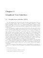
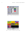
5 Graphical User Interface
53
5.1 Graphical user interface (GUI) . . . . . . . . . . . . . . . . . . . . . . . . . . . . 53
6 Postprocessor Pumaburner
6.1 Introduction . . . . . . . .
6.2 Usage . . . . . . . . . . .
6.3 Namelist . . . . . . . . . .
6.4 HTYPE . . . . . . . . . .
6.5 VTYPE . . . . . . . . . .
6.6 MODLEV . . . . . . . . .
6.7 hPa . . . . . . . . . . . . .
6.8 MEAN . . . . . . . . . . .
6.9 Format of output data . .
6.10 SERVICE format . . . . .
6.11 HHMM . . . . . . . . . .
6.12 HEAD7 . . . . . . . . . .
6.13 MARS . . . . . . . . . . .
6.14 MULTI . . . . . . . . . . .
6.15 Namelist example . . . . .
6.16 Troubleshooting . . . . . .
.
.
.
.
.
.
.
.
.
.
.
.
.
.
.
.
.
.
.
.
.
.
.
.
.
.
.
.
.
.
.
.
.
.
.
.
.
.
.
.
.
.
.
.
.
.
.
.
.
.
.
.
.
.
.
.
.
.
.
.
.
.
.
.
.
.
.
.
.
.
.
.
.
.
.
.
.
.
.
.
.
.
.
.
.
.
.
.
.
.
.
.
.
.
.
.
.
.
.
.
.
.
.
.
.
.
.
.
.
.
.
.
.
.
.
.
.
.
.
.
.
.
.
.
.
.
.
.
.
.
.
.
.
.
.
.
.
.
.
.
.
.
.
.
.
.
.
.
.
.
.
.
.
.
.
.
.
.
.
.
.
.
.
.
.
.
.
.
.
.
.
.
.
.
.
.
.
.
.
.
.
.
.
.
.
.
.
.
.
.
.
.
.
.
.
.
.
.
.
.
.
.
.
.
.
.
.
.
.
.
.
.
.
.
.
.
.
.
.
.
.
.
.
.
.
.
.
.
.
.
.
.
.
.
.
.
.
.
.
.
.
.
.
.
.
.
.
.
.
.
.
.
.
.
.
.
.
.
.
.
.
.
.
.
.
.
.
.
.
.
.
.
.
.
.
.
.
.
.
.
.
.
.
.
.
.
.
.
.
.
.
.
.
.
.
.
.
.
.
.
.
.
.
.
.
.
.
.
.
.
.
.
.
.
.
.
.
.
.
.
.
.
.
.
.
.
.
.
.
.
.
.
.
.
.
.
.
.
.
.
.
.
.
.
.
.
.
.
.
.
.
.
.
.
.
.
.
.
.
.
.
.
.
.
.
.
.
.
.
.
.
.
.
.
.
.
.
.
.
.
.
.
.
.
.
.
.
.
.
.
.
.
.
.
.
.
.
.
.
.
.
.
.
.
.
.
.
.
.
.
.
.
.
.
.
.
.
.
.
.
.
.
.
.
.
.
.
.
.
.
.
.
.
.
.
.
.
.
.
.
.
.
.
.
.
.
.
.
.
.
.
.
.
.
.
.
.
.
.
.
.
.
.
.
.
.
.
.
.
.
.
.
.
.
.
.
.
.
.
.
57
57
57
58
58
58
59
59
59
59
60
60
61
61
61
61
62
7 Graphics
63
7.1 Grads . . . . . . . . . . . . . . . . . . . . . . . . . . . . . . . . . . . . . . . . . 63
7.2 Vis5D . . . . . . . . . . . . . . . . . . . . . . . . . . . . . . . . . . . . . . . . . 66
Bibliography
67
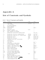
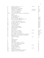
A List of Constants and Symbols
69
A.0.1 List of Constants and Symbols . . . . . . . . . . . . . . . . . . . . . . . . 70
B Puma Codes
75
C Namelist
79
Chapter 1
Installation
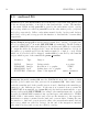
The whole package containing the models ”Planet Simulator” and ”PUMA” along with ”Most”,
the ”Model Starter” comes in a single file, usually named ”Most(n).tar.gz” with (n) specifying
a version number. The following subsection gives an example, assuming version 9.
1.1
Quick Installation
gunzip Most9.tar.gz
tar -xvf Most9.tar
cd Most9
make
most.x
If this sequence of commands produces error messages, consult the ”FAQ” (Frequent Asked
Questions) and README files in the Most9 directory. They are plain text files, that can be
read with the command ”more” or any text editor.
1.2
Directory structure
home/Most9> ls -lg
-rw-r--r--rw-r--r--rwxr-xr-x
-rwxr-xr-x
-rw-r--r--rw-r--r--rwxr-xr-x
drwxr-xr-x
drwxr-xr-x
drwxr-xr-x
1
820
1
550
1
57
1
51
1
83
1 63763
1 66138
8
192
2
136
7
168
FAQ
README
cleanplasim
cleanpuma
makefile
most.c
most.x
plasim
postprocessor
puma
<<<<<<<<<<-
Frequent Ask Questions
Actual information
command clears plasim directories
command clears puma directories
Used to "make" most.x
Source for Most (Model Starter)
Most executable created by "make"
Planet Simulator directory
Postprocessor directory
PUMA directory
The directory structure must not be changed, even empty directories must be kept as they
are, the Most program relies on the existence of these directories!
5
6
CHAPTER 1. INSTALLATION
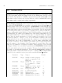
For each model, currently ”Planet Simulator” and ”PUMA” exist a directory with following
subdirectories:
Most9/plasim> ls -lg
drwxr-xr-x
drwxr-xr-x
drwxr-xr-x
drwxr-xr-x
drwxr-xr-x
drwxr-xr-x
2
2
2
2
2
2
128
1824
280
80
928
1744
bin
bld
dat
doc
run
src
<<<<<<-
model executables
build directory
initial and boundary data
documentation, user’s guide, reference manual
run directory
source code
After installation only ”dat”, ”doc” and ”src” contain files, all other directories are empty.
Running ”Most” to configure a model and define an experiment uses the directories in the
following manner:
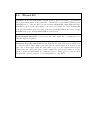
1.3
Model build phase
Most writes an executable shell script to the ”bld” directory and executes it directly hereafter. It copies all necessary source files from ”src” to ”bld” and modifies them according
to the selected parameter configuration. Modification of source code is necessary for vertical and horizontal resolution change and for using more than 1 processor (parallel program
execution). The original files in the ”src” directory are not changed by Most. The program
modules are then compiled and linked using the ”make” command, also issued by Most. Most
provides two different makefiles for the single CPU version or the parallel version (using MPI,
Message Passing Interface). The resolution and CPU parameters are coded into the filename
of the executable, in order to have different names for different versions. E.g. the executable
”most plasim t21 l10 p2.x” is an executable compiled for a horizontal resolution of T21, a vertical resolution of 10 levels and 2 CPU’s. The executable is copied to the model’s ”bin” directory
after building. Each time Most is used to setup a new experiments it checks the ”bin” directory
for a matching executable. If it’s there, it’s used without rebuilding otherwise a new executable
with the selected parameters is created. Rebuilding may be forced by using the cleanplasim
command in the Most directory. The build directory is not cleared after usage. The user may
want to modify the makefile or the build script for his own purposes and start the building
directly by executing ”most plasim build”. For permanent user modifications the contents of
the ”bld” directories have to be copied elsewhere, because each usage of Most overwrites the
contents of ”bld”.
1.4
Model run phase
After building the model with the selected configuration, Most writes or copies all necessary files
to the model’s ”run” directory. These are the executable, initial and boundary data, namelist
files containing the parameter and finally the run script itself. Depending on the exit from Most,
either ”Save & Exit” or ”Run & Exit”, the run script is started from Most and takes control
of the model run. A checkmark on GUI invokes also the the Graphical User Interface for user
1.4. MODEL RUN PHASE
7
control and display of variables during the run. Again all contents of the ”run” directory are
subject of change for the user. But it would be wise to keep changed run setups in other, user
created directories, because each usage of Most will overwrite the contents of the run directory.
Another concept could be to rename user changed files, because Most always generated files
starting with ”most ” and leaves other files untouched.
8
CHAPTER 1. INSTALLATION
Chapter 2
Modules
This is a technical documentation of the PUMA-II model. In the following, the purposes
of the individual modules is given and the general structure and possible input and output
opportunities (namelist, files) are explained.
9
10
CHAPTER 2. MODULES
2.1
fluxmod.f90
General The module fluxmod.f90 contains subroutines to compute the different
surface fluxes and to perform the vertical diffusion. The interface to the main PUMA
module puma.f90 is given by the subroutines fluxini, fluxstep and fluxstop which are
called in puma.f90 from the subroutines prolog, gridpointd and epilog, respectively.
Input/Output fluxmod.f90 does not use any extra input file or output file and is
controlled by the namelist fluxpar which is part of the namelist file puma namelist:
Parameter
NEVAP
Type
Purpose
Integer Switch for surface evaporation (0 = off,
1 = on)
NSHFL
Integer Switch for surface sensible heat flux
(0 = off, 1 = on)
NSTRESS
Integer Switch for surface wind stress (0 = off,
1 = on)
NTSA
Integer Switch for computing the near surface
air temperature which is used for the
Richardson number (1 = potential temperature, 2 = virtual potential temperature)
NVDIFF
Integer Switch for vertical diffusion (0 = off,
1 = on)
VDIFF LAMM Real
Tuning parameter for vertical diffusion
VDIFF B
Real
Tuning parameter for vertical diffusion
VDIFF C
Real
Tuning parameter for vertical diffusion
VDIFF D
Real
Tuning parameter for vertical diffusion
Default
1
1
1
2
1
160.
5.
5.
5.
Structure Internally, fluxmod.f90 uses the FORTRAN-90 module fluxmod, which
uses the global common module pumamod from pumamod.f90. Subroutine fluxini
reads the namelist and, if the parallel version is used, distributes the namelist parameters to the different processes. Subroutine fluxstep calls the subroutine surflx to
compute the surface fluxes and calls the subroutine vdiff to do the vertical diffusion.
Subroutine fluxstop is a dummy subroutine since there is nothing to do to finalize
the computations in fluxmod.f90. The computation of the surface fluxes in surflx
is spitted into several parts. After initializing the stability dependent transfer coefficients, the subroutines mkstress, mkshfl and mkevap do the computations which
are related to the surface wind stress, the surface sensible heat flux and the surface
evaporation, respectively.
11
2.2
miscmod.f90
General The module miscmod.f90 contains miscellaneous subroutines which do not
fit well to other modules. The interface to the main PUMA module puma.f90 is given
by the subroutines miscini, miscstep and miscstop which are called in puma.f90
from the subroutines prolog, gridpointd and epilog, respectively. A subroutine to
eliminate spurious negative humidity and an optional subroutine to relax the upper
level temperature towards a prescribed distribution is included in miscmod.f90.
Input/Output miscmod.f90 does not use any extra output file. If the relaxation is
switched on, a climatological annual cycle of the prescribed upper level temperature
distribution [K] is read from the external file CLIMATEFILE (see namelist). The
file format is formatted SERVICE format with (8I10) for the headers and (8E12.6)
for the temperature fields. To assign the field, the header needs to have the header
information code 130, level 1 and a date identifier of the form yymmdd or mmdd
where mm goes from 01 to 12 (January to December). Fields which are not needed
will be skipped. The module is controlled by the namelist miscpar which is part of
the namelist file puma namelist:
Parameter
Type
NFIXER
Integer
Purpose
default
Switch for correction of neg1
ative moisture (0 = off , 1=
on)
NUDGE
Integer
Switch for temperature re0
laxation in the uppermost
level (0 = off , 1= on)
TNUDGE
Real
Time scale [d] of the tem10.
perature relaxation
CLIMATEFILE Character Name of the file containing surface parameter
the prescribed temperature
distribution
Structure Internally, miscmod.f90 uses the FORTRAN-90 module miscmod, which
uses the global common module pumamod from pumamod.f90. Subroutine miscini
reads the namelist and, if the parallel version is used, distributes the namelist parameters to the different processes. If the relaxation is switched on, the climatological
temperature is read from CLIMATEFILE and distributed to the processors. Subroutine miscstep calls the subroutine fixer to eliminate spurious negative humidity
arising from the spectral method and, if the relaxation is switched on, calls the subroutine mknudge to do the temperature nudging. Subroutine miscstop is a dummy
subroutine since there is nothing to do to finalize the computations in miscmod.f90.
12
CHAPTER 2. MODULES
2.3
surfmod.f90
General The module surfmod.f90 deals as an interface between the atmospheric part
of the model and modules, or models, for the land and the oceans. The interface
to the main PUMA module puma.f90 is given by the subroutines surfini, surfstep
and surfstop which are called in puma.f90 from the subroutines prolog, gridpointd
and epilog, respectively. Calls to subroutines named landini, landstep and landstop
and seaini, seastep and seastop provide the interface to land and the ocean modules,
respectively.
Input/Output surfmod.f90 reads the land-sea mask [frac.] and the orography (surface geopotential) [m2 /s2 ] from file INPUTFILE (see namelist). The file format is
formatted SERVICE format with (8I10) for the headers and (8E12.6) for the fields.
To assign the fields, the headers need to have the header information code 129 for
the surface geopotential and 172 for the land-sea mask (1. = land; 0. = sea). Fields
which are not needed will be skipped. surfmod.f90 is controlled by the namelist
surfpar which is part of the namelist file puma namelist:
Parameter
Type
NSURF
Integer
NOROMAX Integer
OROSCALE Real
INPUTFILE Character
Purpose
Debug switch
Resolution of orography
Scaling factor for orography
Name of the input file
default
not active
NTRU
1.0
surface parameter
Structure Internally, surfmod.f90 uses the FORTRAN-90 module surfmod, which
uses the global common module pumamod from pumamod.f90. Subroutine surfini
reads the namelist and, if the parallel version is used, distributes the namelist parameters to the different processes. If the run is not started from a restart file
(NRESTART from namelist inpof puma.f90 is 0), the land-sea-mask and the orography are read from file INPUTFILE. According to the namelist input, the orography
is scaled by OROSCALE, transfered into spectral space and truncated to NOROMAX. Calls to subroutines landini and seaini are the interfaces to the respective
initialization routines contained in the land and ocean modules. During the run,
the interface to land and ocean is given by calls to the external subroutines landstep
and seastep, which are called by surfstep. At the end of the integration, interface
subroutines landstop and seastop are called by surfstop.
13
2.4
fftmod.f90
General The module fftmod.f90 contains all subroutines necessary to perform the
fast fourier transformation and its inverse. The interface to the main PUMA module
puma.f90 and to other modules (at the moment surfmod.f90, legmod.f90 and rainmod.f90) is given by the subroutines gp2fc and fc2gp which are called in puma.f90
from the subroutines gridpointa and gridpointd, in surfmod.f90 from surfini, in legmod.f90 from sp2gp, and in rainmod.f90 from mkdqdtgp.
Input/Output fftmod.f90 does not use any extra input file or output file. No
namelist input is required.
Structure Internally, fftmod.f90 uses the FORTRAN-90 module fftmod, which uses
no other modules. Subroutine gp2fc performs the transformation from grid point
space into fourier space while the subroutine fc2gp does the transformation from
fourier space into grid point space. Both routines use several subroutines to do the
direct or indirect transformation for different factors. When gp2fc or fc2gp is called
the first time, fftini is called to do the initialization of the FFT.
14
CHAPTER 2. MODULES
2.5
landmod.f90
General The module landmod.f90 contains parameterizations for land surface and
soil processes which include the simple biome model SIMBA and a model for the
river runoff. The interface to PUMA is given via the module surfmod.f90 by the
subroutines landini, landstep and landstop which are called in surfmod.f90 from the
subroutines surfini, surfstep and surfstop, respectively.
Input/Output landmod.f90 reads several surface and soil parameters either from
the initial file STARTFILE (see namelist) or from the restart file land restart
which is written at the end of an integration. STARTFILE contains different surface fields which are needed for initialization. The file format is formatted SERVICE
format with (8I10) for the header and (8E12.6) for the fields. The file may include
the following fields: surface geopotential (orography) [m2 /s2 ], land-sea mask [frac.],
surface roughness [m], background albedo [frac.], glacier mask [frac.], bucket size [m],
soil temperature [K], climatological annual cycle of the surface temperature [K], climatological annual cycle of the soil wetness [m]. To assign the fields, the headers
need to have the header information code 129 for surface geopotential, code 172 for
the land-sea mask (1. = land; 0. = sea), 173 for the surface roughness, 174 for the
background albedo, 232 for the glacier mask (1. = glacier; 0. = no glacier), 229 for
the bucket size, 209 for the soil temperature, 169 for the surface temperature and
140 for the soil wetness. for the climatological annual cycles of surface temperature
and soil wetness, a date identifier of the form yymmdd or mmdd where mm goes
from 01 to 12 (January to December) is required. Fields which are not needed will
be skipped. If there are some fields not present in the STARTFILE default values
will be used which can be set in the namelist. The use of some fields depend on
the setting of some namelist parameters. The restart file land restart is an unformatted file which contains all variables needed to continue the run. landmod.f90 is
controlled by the namelist landpar given in the namelist file land namelist:
Parameter
Type
NLANDT
Integer
Purpose
Switch for surface temperature (1 = computed; 2 = climatology)
NLANDW
Integer Switch for soil wetness
(1 = computed; 2 = climatology)
NBIOME
Integer Switch for biome model
SIMBA (1 = on ; 0 = off)
ALBLAND
Real
Background albedo
DZ0LAND
Real
Roughnesslength [m]
DRHSLAND Real
Wetness factor
ALBSMIN
Real
Minimum albedo for snow
ALBSMAX
Real
Maximum albedo for snow
Default
1
1
0
0.2
2.0
0.25
0.4
0.8
15
Parameter
Type
ALBGMIN
Real
Purpose
Default
Minimum
albedo
for
0.6
glaciers
ALBGMAX Real
Maximum
albedo
for
0.8
glaciers
WSMAX
Real
Maximum field capacity of
0.5
soil water (bucket size) [m]
DRHSFULL Real
Threshold above which wet0.4
ness factor is 1
DZGLAC
Real
Threshold of orography to
-1.0
be glacier (-1.0 = none) [m]
DZTOP
Real
Thickness of the uppermost
0.2
soil layer [m]
DSOILZ(5)
Real Array Soil layer thicknesses [m]
0.4,0.8,1.6,3.2,6.4
STARTFILE Character Initialization file
surface parameter
Structure Internally, landmod.f90 uses the FORTRAN-90 module landmod, which
uses the global common module pumamod from pumamod.f90. Subroutine landini
reads the namelist and, if the parallel version is used, distributes the namelist parameters to the different processes. If the run is not started from a restart file
(NRESTART from namelist inp of puma.f90is 0), the initialization file STARTFILE is being read. The soil and the river runoff are initialized via soilini and
roffini and different variables are set according to the values given by the namelist
or the STARTFILE. If it is a restart (NRESTART = 1), the restart records are
being read from land restart. Additionally, the climatological surface temperatures and soil wetnesses are updated from STARTFILE if NRESTART = 2. If
NRESTART = 3 (special application) the bucket size, the roughness length and the
albedo are set to the values given in the namelist. Subroutine landstep computes
new surface and soil values via soilstep which calls tands and wandr for the heat and
water budgets, respectively. If NLANDT and/or NLANDW are set to 0, climatological values are used for the surface temperature and the soil wetness. Via roffstep
the river runoff is computed. Finally the biome model simbastep is called. The land
model is finalized by landstop which writes the restart record to land restart.
16
CHAPTER 2. MODULES
2.6
legmod.f90
General The module legmod.f90 contains all subroutines necessary to perform the
Legendre transformation and its inverse. The interface to the main PUMA module
puma.f90 and to other modules (at the moment surfmod.f90 and rainmod.f90) is given
by the subroutines legini, gauaw, sp2fl, invlega, invlegd, fc2sp, dirlega, dirlegd, fc3sp,
uv2dv and sp2gp which are called in puma.f90 from the subroutines prolog, gridpointa
and gridpointd, in surfmod.f90 from surfini, and in rainmod.f90 from mkdqdtgp.
Input/Output legmod.f90 does not use any extra input file or output file. No
namelist input is required
Structure Internally, legmod.f90 uses the FORTRAN-90 module legmod, which
uses the global common module pumamod from pumamod.f90. Subroutine legini
does the initialization. Subroutine gauaw computes the Gaussian latitudes and the
corresponding weights. Subroutine sp2fl performs the transformation from spectral
to fourier space for multilevel fields. The Subroutines invlega and invlegd contain the
transformations from spectral to fourier space for all varibles which are needed in
the adiabatic and in the diabatic part of the model, respectively. Subroutine fc2sp
does the transformation from fourier to spectral space. The Subroutines dirlega and
dirlegd contain the transformations from fourier to spectral space for the tendencies
computed in the adiabatic and in the diabatic part of the model, respectively. Subroutine uv2dv transforms the fourier coefficients of the zonal and meridional wind
components to spectral coefficients of divergence and vorticity.
17
2.7
mpimod.f90 and mpimod dummy.f90
General The module mpimod.f90 contains interface subroutines to the MPI (Message Passing Interface) needed for massive parallel computing. Several MPI routines are called from the module. The interface to other modules are given by numerous subroutines which name starts with mp. Subroutines from mpimod.f90 are
called in fluxmod.f90, icemod.f90, landmod.f90, miscmod.f90, oceanmod.f90, oceanmod50.f90, outmod.f90, puma.f90, radmod.f90, rainmod.f90, seamod.f90, surfmod.f90
and visumod.f90. The module mpimod dummy.f90 is used instead of mpimod.f90 for
simulations on a single processor. mpimod dummy.f90 contains subroutines having
the same name as the corresponding routine in mpimod.f90. However, there is no
interface to MPI present in these routines and most of them are dummies.
Input/Output mpimod.f90 and mpimod dummy do not use any extra input file or
output file. No namelist input is required
Structure Internally, mpimod.f90 uses the FORTRAN-90 module mpimod, which
uses the global common module pumamod from pumamod.f90 and the MPI module
mpi. mpimod dummy.f90 does not use any module. The following subroutines are
included in mpimod.f90:
Subroutine
Purpose
mpbci
mpbcin
mpbcr
mpbcrn
mpscin
mpscrn
mpscgp
mpgagp
mpgallgp
mpscsp
mpgasp
mpgacs
mpgallsp
mpsum
mpsumsc
mpsumr
mpsumbcr
mpstart
mpstop
broadcast 1 integer
broadcast n integers
broadcast 1 real
broadcast n reals
scatter n integers
scatter n reals
scatter grid point field
gather grid point field
gather grid point field to all
scatter spectral field
gather spectral field
gather cross section
gather spectral field to all
sum spectral field
sum and scatter spectral field
sum n reals
sum and broadcast n reals
initialize MPI
finalize MPI
18
CHAPTER 2. MODULES
Subroutine
Purpose
mpreadgp
mpwritegp
mpwritegph
mpreadsp
mpwritesp
mpi info
read and scatter grid point field
gather and write grid point field
gather and write (with header) grid point field
read and scatter spectral field
gather and write spectral field
give information about setup
19
2.8
outmod.f90
General The module outmod.f90 controls the data output of the model. The interface to the main PUMA module puma.f90 is given by the subroutines outini, outgp,
outsp, outreset and outaccu which are called in puma.f90 from the subroutines prolog
and master.
Input/Output outmod.f90 writes the output data to the file puma output which
is an unformatted file. puma output is designed to be post processed by the
AFTERBURNER program (see EDI) which converts the model variables to useful
output in user friendly format. There is no separate namelist for outmod.f90 but
some parameter of namelist inp of puma.f90 are used to control the format and the
output interval.
Structure Internally, outmod.f90 uses the global common module pumamod from
pumamod.f90 in several subroutines. Subroutine outini does the initialization. Subroutines outgp and outsp write the grid point and the spectral fields to the output
file puma output. outaccu accumulates some output variables over the output
interval. outreset resets the accumulated arrays to zero.
20
CHAPTER 2. MODULES
2.9
puma.f90
General The module puma.f90 is the main module of the model. It includes the
main program puma and controls the run. From puma.f90 the interface routines
to the modules miscmod.f90, fluxmod.f90, radmod.f90, rainmod.f90, surfmod.f90 are
called. The output is done by calling the interface routines to outmod.f90. In
addition, the adiabatic tendencies and the horizontal diffusion are computed in
puma.f90. To do the necessary transformations, calls to the modules fftmod.f90 and
legmod.f90 are used.
Input/Output puma.f90 does not use any extra input file or output file. A diagnostic print out is written on standard output. puma.f90 is controlled by the namelist
inp which is part of the namelist file puma namelist:
Parameter
Type
KICK
Integer
Purpose
Default
Switch for initial white
1
noise disturbance on surface pressure (0 = none;
1 = global; 2 = hemispherically symmetric; 3 = one
wavenumber only)
NAFTER
Integer
Time interval for output
12
[time steps]
NCOEFF
Integer
Number of spectral coeffi0
cients in diagnostic print
out
NDEL(NLEV) Integer Array Order of the horizontal dif- NLEV · 2
fusion
NDIAG
Integer
Time interval for diagnostic
12
print out [time steps]
NEXP
Integer
Experiment identifier
0
NEXPER
Integer
Switch for predefined exper0
iments (not used)
NKITS
Integer
Number of initial explicit
3
Euler time steps
NRESTART
Integer
Switch for restart (0 = ini0
tial run; 1 = normal
restart; 2 = restart plus update of surface climatology;
3 = restart plus update of
surface parameter (see landmod.f90))
NRUN
Integer
Number of time steps to be
0
run
NSTEP
Integer
Current time step (replaced
0
by restart record)
21
Parameter
Type
Purpose
NSTOP
NTSPD
Integer
Integer
NDAYS
Integer
NEQSIG
Integer
NPRINT
Integer
NPRHOR
Integer
NPACKSP
Integer
NPACKGP
Integer
NRAD
Integer
NFLUX
Integer
NDIAGGP
Integer
NDIAGSP
Integer
NDIAGCF
Integer
Finishing time step
0 (= not active)
Number of time steps per
24
day
Number of days to be run
0
(overwrites NRUN if > 0)
Switch for non equally
1
spaced
sigma
levels
(1 = non equally spaced;
1 = equally spaced)
Switch for extended debug
0
print out (0 = off; 1 = on;
2 = very extended)
Number of the grid point to
0
be used for very extended
debug print out
Switch for spectral output
1
(0 = normal; 1 = compressed)
Switch for grid point out1
put (0 = normal; 1 = compressed)
Switch
for
radiation
1
(0 = off; 1 = on)
Switch for surface fluxes
1
and
vertical
diffuson
(0 = off; 1 = on)
Switch for additional di0
agnostic grid point output
(0 = off; 1 = on)
Switch for additional di0
agnostic spectral output
(0 = off; 1 = on)
Switch for additional cloud
0
forcing diagnostic (0 = off;
1 = on)
Number of additional diag0
nostic 2-d grid point output
(0 = off; 1 = on)
Number of additional diag0
nostic 3-d grid point output
(0 = off; 1 = on)
Number of additional diag0
nostic 2-d spectral output
(0 = off; 1 = on)
Number of additional diag0
nostic 3-d spectral output
(0 = off; 1 = on)
NDIAGGP2D Integer
NDIAGGP3D Integer
NDIAGSP2D
Integer
NDIAGSP3D
Integer
Default
22
CHAPTER 2. MODULES
Parameter
Type
Purpose
NDL(NLEV)
Integer Array
NHDIFF
Integer
NTIME
Integer
NPERPETUAL
Integer
DTEP
Real
DTNS
Real
DTROP
Real
DTTRP
Real
TGR
Real
TDISSD(NLEV)
Real Array
TDISSZ(NLEV)
Real Array
TDISST(NLEV)
Real Array
TDISSQ(NLEV)
Real Array
PSURF
Real
RESTIM(NLEV)
Real Array
Switch for diagnostic print
out of a level (0 = off;
1 = on)
Cut off wave number for
horizontal diffusion
Switch for CPU time diagnostics (0 = off; 1 = on)
Switch for perpetual simulations (0 = annual cycle;
>0 = day of the year)
Equator to pole temperature difference [K] for Newtonian cooling (usually not
used)
North pole to south pole
temperature difference [K]
for Newtonian cooling (usually not used)
Tropopause height [m] for
Newtonian cooling (usually
not used)
Smoothing
of
the
tropopause [K] for Newtonian cooling (usually not
used)
Surface temperature [K] for
Newtonian cooling (usually
not used)
time scale [d] for the horizontal diffusion of divergence
time scale [d] for the horizontal diffusion of vorticity
time scale [d] for the horizontal diffusion of temperature
time scale [d] for the horizontal diffusion of moisture
Global averaged sea level
pressure [Pa]
Time scale [d] for Newtonian cooling (usually not
used)
Default
NLEV · 0
15
0
0
0.0
0.0
12000.0
2
280
NLEV · 0.2
NLEV · 1.1
NLEV · 5.6
NLEV · 5.6
101325.00
NLEV · 0.0
23
Parameter
Type
Purpose
Default
Reference temperature used NLEV · 250.0
in the discretization scheme
TFRC(NLEV) Real Array Time scale [d] for Rayleigh NLEV · 0.0
friction (0.0 = off)
T0(NLEV)
Real Array
Structure Internally, fluxmod.f90 uses the FORTRAN-90 global common module
pumamod from pumamod.f90. After starting MPI, the main program puma calls
prolog for initializing the model. Then, master is called to do the time stepping.
Finally, subroutine epilog finishes the run. In subroutine prolog, calls to different
subroutines, which are part of puma.f90 or are provided by other modules, initialize various parts of the model: gauaw and inilat build the grid, readnl reads the
namelist and sets some parameter according to the namelist input, initpm and initsi
initialize some parameter for the physics and the semi implicit scheme, respectively.
outini starts the output. If NRESTART > 0, the restart record is read by restart,
otherwise initfd sets the prognostic variables to their initial values. calls to miscini
fluxini, radini, rainini and surfini start the initialization of the respective external
modules. Finally, the global averaged surface pressure is set according to PSURF
and the orography. Subroutine master controls the time stepping. First, if its not
a restart, initial NKITS explicit forward timesteps are performed. The main loop
is defined by calling gridpointa for the adiabatic tendencies, spectrala to add the
adiabatic tendencies, gridpointd for the diabatic tendencies (which are computed by
the external modules), spectrald to add the diabatic tendencies and the interface
routines to the output module outmod.f90. The run is finalized by subroutine epilog
which writes the restart records and calls the respective interface routines of the
external modules.
24
CHAPTER 2. MODULES
2.10
pumamod.f90
General The module pumamod.f90 contains all parameters and variables which may
be used to share information between puma.f90 and other modules. No subroutines
or programs are included.
Input/Output pumamod.f90 does not use any extra input file or output file. No
namelist input is required
Structure Internally, pumamod.f90 is a FORTRAN-90 module named pumamod.
Names for global parameters, scalars and arrays are declared and, if possible, values
are preset.
25
2.11
radmod.f90
General The module radmod.f90 contains subroutines to compute radiative energy
fluxes and the temperature tendencies due to long wave and short wave radiation.
The interface to the main PUMA module puma.f90 is given by the subroutines
radini, radstep and radstop which are called in puma.f90 from the subroutines prolog,
gridpointd and epilog, respectively.
Input/Output radmod.f90 does not use an extra output file. If the Switch for ozone
(NO3, see namelist) is set to 2 (externally prescribed), the climatological cycle of
the ozone distribution is read from the external file OZONEFILE which name is
given in the namelist. The file format is formatted SERVICE format with (8I10) for
the header and (8E12.6) for the fields. To assign the fields, the headers need to have
the header information code 200, level going from 1 to NLEV and a date identifier
of the form yymmdd or mmdd where mm goes from 01 to 12 (January to December).
radmod.f90 is controlled by the namelist radpar which is part of the namelist file
puma namelist:
Parameter
Type
NDCYCLE
Integer
NO3
CO2
GSOL0
IYRBP
NSWR
NLWR
NSOL
NSWRCL
NRSCAT
RCL1(3)
Purpose
Default
Switch for diurnal cycle of
0
insolation (0 = off, 1 = on)
Integer
Switch for ozone (0 = off,
1
1 = idealized distribution,
2 = externally presrcibed)
Real
CO2 concentration [ppmv]
360.0
2
Real
Solar constant [W/m ]
1367.0
Integer
Year PB (reference is 1950)
-50
to calculate orbit from
Integer
Switch for short wave radi1
ation (0 = off, 1 = on)
Integer
Switch for long wave radia1
tion (0 = off, 1 = on)
Integer
Switch for incoming solar
1
radiation (0 = off, 1 = on)
Integer
Switch for computed short
1
wave
cloud
properties
(0 = off, 1 = on)
Integer
Switch for Rayleigh scatter1
ing (0 = off, 1 = on)
Real Array Prescribed cloud albedos 0.15,0.30.0.60
[frac.] for high, middle and
low level clouds (spectral
range 1)
26
CHAPTER 2. MODULES
Parameter
Type
RCL2(3)
Real Array
Purpose
Default
Prescribed cloud albedos 0.15,0.30.0.60
[frac.] for high, middle and
low level clouds (spectral
range 2)
ACL2(3)
Real Array Prescribed cloud absorptiv- 0.05,0.10.0.20
ities [frac.] for high, middle
and low level clouds (spectral range 2)
CLGRAY
Real
Prescribed grayness of
-1.0
clouds (-1.0 = computed)
TPOFMT
Real
Tuning for point of mean
0.15
transmission
ACLLWR
Real
Mass absorption coefficient
0.1
for clouds (long wave)
TSWR1
Real
Tuning of cloud albedo
0.035
(spectral range 1)
TSWR2
Real
Tuning of cloud back scat0.04
tering (spectral range 2)
TSWR3
Real
Tuning of cloud single
0.006
scattering albedo (spectral
range 2)
OZONEFILE Character File for externally preozone.dat
scribed ozone distribution
Structure Internally, radmod.f90 uses the FORTRAN-90 module radmod, which
uses the global common module pumamod from pumamod.f90. Additionally, the
FORTRAN-90 module orbparam is used. Subroutine radini reads the namelist and,
if the parallel version is used, distributes the namelist parameters to the different
processes. Orbital parameters are computed by calling orb params. If NO3 is set to
2, the ozone distribution is read from OZONEFILE. Subroutine radstep calls the
subroutines solang and mko3 to compute the cosine of the solar angle and the ozone
distribution, respectively. The short wave radiative fluxes are calculate in swr while
the long wave radiative fluxes are computed in lwr. Subroutine radstop is a dummy
subroutine since there is nothing to do to finalize the computations in radmod.f90.
27
2.12
rainmod.f90
General The module rainmod.f90 contains subroutines to compute large scale and
convective precipitation and the related temperature tendencies. In addition, a
parameterization of dry convective mixing of temperature and moisture is included
and cloud cover is diagnosed. The interface to the main PUMA module puma.f90 is
given by the subroutines rainini, rainstep and rainstop which are called in puma.f90
from the subroutines prolog, gridpointd and epilog, respectively.
Input/Output rainmod.f90 does not use any extra input or output file and is controlled by the namelist rainpar which is part of the namelist file puma namelist:
Parameter
Type
KBETTA
Integer
Purpose
Default
Switch for betta in Kuo
1
parameterization (0 = off,
1 = on)
NPRL
Integer
Switch for large scale pre1
cipitation (0 = off, 1 = on)
NPRC
Integer
Switch for convective pre1
cipitation (0 = off, 1 = on)
NDCA
Integer
Switch for dry convective
1
adjustment (0 = off, 1 = on)
RCRIT(NLEV) Real Array Critical relative humidity computed
for cloud formation
CLWCRIT1
Real
Critical
vertical
veloc-0.1
ity for cloud formation
[Pa/s] (not active if
CLWCRIT2 > CLWCRIT1)
CLWCRIT2
Real
Critical
vertical
veloc0.0
ity for cloud formation
[Pa/s] (not active if
CLWCRIT2 > CLWCRIT1)
Structure Internally, rainmod.f90 uses the FORTRAN-90 module rainmod, which
uses the global common module pumamod from pumamod.f90. Subroutine rainini
reads the namelist and, if the parallel version is used, distributes the namelist parameters to the different processes. Subroutine rainstep calls the subroutine mkdqdtgp
to obtain the adiabatic moisture tendencies in grid point space, which are needed for
the Kuo parameterization. kuo is called to compute the convective precipitation and
the respective tendencies. Dry convective adjustment is performed in mkdca. Large
scale precipitation is computed in mklsp. Finally, diagnostic clouds are calculated
in mkclouds. Subroutine radstop is a dummy subroutine since there is nothing to do
to finalize the computations in radmod.f90.
28
CHAPTER 2. MODULES
2.13
seamod.f90
General The module seamod.f90 is the interface from the atmosphere to the ocean
and the sea ice. The interface to the main PUMA module puma.f90 is given by
the subroutines seaini, seastep and seastop which are called in puma.f90 from the
subroutines prolog, gridpointd and epilog respectively.
Input/Output seamod.f90 reads different surface parameters either from the file
SSTFILE (see namelist) and the file ocean parameter or from the restart file
sea restart which is written at the end of an integration.. The files formats are
unformatted for the restart file, formatted SERVICE format with (8I10) for the
header and (8E12.6) for the fields for SSTFILE and formatted EXTRA format
with (4I10) for the header and (6(1X,E12.6)) for the fields for ocean parameter.
The file SSTFILE may include the following fields: The climatological annual cycle of the surface temperature [K] and the climatological annual cycle of the sea
ice compactness [frac.]. To assign the fields, the headers need to have the header
information code 169 for surface temperature and code 210 for the compactness
(1 = ice; 0. = open water). a date identifier of the form yymmdd or mmdd where
mm goes from 1 to 12 (January to December) is required. Fields which are not
needed will be skipped. The file ocean parameter includes the following fields:
The climatological annual cycle of the sea surface temperature [K], the climatological
annual cycle of the mixed layer depth [m] and the climatological average of the deep
ocean temperature [m]. To assign the fields, the order must be as described above
(no header information is used). The restart file sea restart contains all variables
needed to continue the run. seamod.f90 is controlled by the namelist seapar given
in the namelist file sea namelist:
Parameter
Type
ALBSEA
ALBICE
DZ0SEA
Real
Real
Real
Purpose
Default
Albedo for ice free ocean
0.069
Maximum albedo for sea ice
0.7
Minimum roughness length 1.0 · 10−5
[m] for ice free ocean
DZ0ICE
Real
Roughness length [m] for 1.0 · 10−3
sea ice
DRHSSEA Real
Wetness factor for ice free
1.0
ocean
DRHSICE Real
Wetness factor for sea ice
1.0
NOCEAN Integer Switch for ocean model
1
(0 = climatological SST,
1 = ocean model)
NICE
Integer Switch for sea ice model
1
(0 = climatological, 1 = sea
ice model)
29
Parameter
Type
NCPL ICE OCEAN
Integer
NCPL ATMOS ICE
TDEEPSEA
DHICEMIN
SSTFILE
Purpose
Default
ice-ocean coupling time
32
steps
Integer ice atmosphere coupling
1
time steps
Real
Homogeneous deep ocean
0.0
temperature [K]
Real
Minimum sea ice thickness
0.1
[m]
FILE
File with SST data
surface parameter
Structure Internally, seamod.f90 uses the FORTRAN-90 module seamod, which
uses the global common module pumamod from pumamod.f90. Subroutine seaini
reads the namelist and, if the parallel version is used, distributes the namelist parameters to the different processes. The coupling interface routines in intermod atm.f90
are initialized by calling cplinit. If it is not a restart (i.e. if NRESTART from
inp of puma.f90 is 0), the files SSTFILE and ocean parameter are being read.
The climatological sea ice compactness is converted to a sea ice thickness as initial
condition and additional surface parameters are set. If it is a restart, the restart
file sea restart is read. Subroutine seastep accumulates the variables used for the
coupling between the atmosphere and the ocean. The coupling is done via the sea
ice model. There is no direct connection between atmosphere and ocean model. If
there is no sea ice, the coupling quantities are passed through the ice model without
changes. A call to cplexchange ice from module intermod atm.f90 transfers the atmospheric coupling fluxes to the sea ice model and gets the sea ice and ocean surface
data back. After the call, additional surface parameter are computed. Subroutine
seastop finalizes the run and writes the restart records.
30
2.14
CHAPTER 2. MODULES
Files
2.15. SEA ICE AND OCEAN MODULES
2.15
31
Sea ice and ocean modules
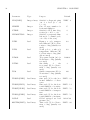
This section describes the modules that represent sea ice and ocean and the necessary interfaces
between these modules and the atmospheric modules. Conceptually, the sea ice model lies
inbetween the atmosphere model and the ocean model. Thus, the PUMA main part and the
ocean model are both coupled to the sea ice model, but not directly to each other. The sea ice
model decides whether a given gridpoint is covered with ice or not, in the latter case, it merely
functions as passing the ocean fluxes to the atmosphere and vice versa. The parameters that
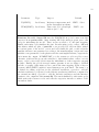
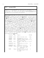
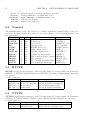
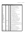
are exchanged are listed in Table 2.1. The sea ice and ocean model use a time step of one day.
Thus, atmospheric coupling to the sea ice model is performed every 32 time steps, while the
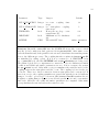
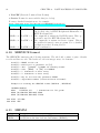
sea ice and ocean model are coupled every time step. The coupling scheme is shown in Fig.
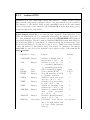
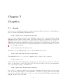
2.1. Fig. 2.2 shows how the subroutines are placed when no external coupler is used.
Parameter
Atmosphere ← → Ice
Ice cover
←
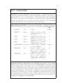
Ice thickness
←
Snow thickness
←
Surface temperature
←
Deep sea temperature
−
Mixed layer depth
−
Net precipitation, runoff
→
Salinity
−
Melt and freeze volume
−
Heat fluxes
→
d(Heat fluxes)/dT
→
Radiation
→
Wind stress
→
Ice ← → Ocean
−
→
→
←
←
←
→
←
→
→
−
−
→
Table 2.1: Parameters to be exchanged between models. Arrows denote the direction in which
the parameter is passed, e.g. the atmosphere receives ice cover information from the ice model.
32
CHAPTER 2. MODULES
Timesteps
32
1
Timesteps
1
1
ATMOSPHERE
net precipitation,
runoff,
total heatflux,
sensible heatflux,
radiation,
wind stress
surface temperature,
ice cover,
snow thickness,
ice thickness
SEA ICE
net precipitation,
runoff,
total heatflux,
wind stress,
freeze and melt volume
sea surface temperature,
deep sea temperature,
mixed layer depth,
salinity
OCEAN
Figure 2.1: Schematic illustration of the model coupling.
2.15. SEA ICE AND OCEAN MODULES
33
FLOW DIAGRAM
ATMOSPHERE − ICE − OCEAN
EXCHANGE
PUMA MAIN LOOP
puma.f90
SURFSTEP
surfmod.f90
LANDSTEP
landmod.f90
SEASTEP
seamod.f90
CPLEXCHANGE_ICE
intermod_atm.f90
ICESTEP
icemod.f90
CPLEXCHANGE_OCEAN
iintermod_ice.f90
CPLEXCHANGE_ATMOS
intermod_ice.f90
OCEANSTEP
oceanmod.f90
Figure 2.2: Subroutine flow when no external coupler is used.
34
CHAPTER 2. MODULES
2.15. SEA ICE AND OCEAN MODULES
2.15.1
seamod.f90
General The module seamod.f90 deals as an interface between the atmospheric part of the
model and modules for the ocean and sea ice. The basic subroutines seaini, seastep and
seastop are called by the the subroutines surfini, surfstep and surfstop, respectively (see
module surfmod.f90). See the reference guide, section (heiko.coupling) for a visualization
of the module coupling structure.
Input/Output seamod.f90 needs the parameter file surface_parameter to read the
climatological sea surface temperature and ice cover as well as ocean_parameter, which
contains climatological mixed layer depth and the Levitus 400 m temperature. As output
data, the file sea_restart is produced at the end of a run. In the case of a restart, this
file is required to be read in by the module. The namelist seapar, which is contained in
the file sea_namelist, is defined as:
Parameter
Type
Purpose
default
ALBSEA
REAL
Albedo for open water
0.069
ALBICE
REAL
Max. albedo for sea ice
0.7
DZ0SEA
REAL
Roughness length sea
1.5·10−5 m
DZ0ICE
REAL
Roughness length ice
1.0·10−3 m
DRHSSEA
REAL
Wetness factor sea
1.0
DRHSICE
REAL
Wetness factor ice
1.0
NOCEAN
INTEGER Ocean model (1) or cli- 1
matology (0)
NICE
INTEGER Sea ice model (1) or cli- 1
matology (0)
NCPL_ICE_OCEAN INTEGER Ice Ocean coupling time 1
steps
NCPL_ATMOS_ICE INTEGER Atmosphere Ice coupling 32
time steps
SSTFILE
CHAR*80 file containing climatology ”surface_parameter”
Structure Internally, seamod.f90 uses the FORTRAN-90 module seamod, which uses the
global common module pumamod from pumamod.f90. Subroutine seaini reads the namelist
and, if the parallel version is used, distributes the namelist parameters to the different
processes. If the run is not started from a restart file (NRESTART from namelist inp is
0), the sea surface temperature and the ice cover is read from the surface_parameter
file. Ice thickness is computed from ice cover. Additionally, mixed layer depth and the
400 m Levitus temperature is read from the file ocean_parameter. Climatology and
namelist information is passed to the ice and ocean modules via the external subroutines iceini (in icemod.f90) and oceanini (in oceanmod.f90 or oceanmod50.f90). Every
NCPL_ATMOS_ICE time steps, seastep calls the ice module via the external subroutine
cplexchange_ice (defined in intermod_atm.f90). At the end of the integration, seastop
writes the restart information into file sea_restart.
35
36
CHAPTER 2. MODULES
2.15.2
intermodatm.f90
General The module intermod_atm.f90 contains subroutines that exchange
information between the atmospheric module and the sea ice module. If an
external coupler is used with an independent sea ice / ocean model, the module
is replaced e.g. by mpccimod_atm.f90 which contains the relevant subroutines
for the MpCCI coupler.
Input/Output intermod_atm.f90 does not use any extra input file or output
file.
Structure The subroutines cplstart, cplinit, cplstop are dummy routines that
are real subroutines only in the case of external coupling. The subroutine
cplexchange_ice, which is called by seastep in module seamod.f90, calls the
external subroutine icestep (defined in icemod.f90). It then copies the ice /
ocean data to the relevant PUMA variables.
2.15. SEA ICE AND OCEAN MODULES
2.15.3
intermodice.f90
General The module intermod_ice.f90 contains subroutines that exchange information between the sea ice module and the ocean and atmosphere module.
If an external coupler is used with an independent sea ice / ocean model,
the module is replaced e.g. by mpccimod_ice.f90 which contains the relevant
subroutines for the MpCCI coupler.
Input/Output intermod_ice.f90 does not use any extra input file or output
file.
Structure The subroutine cplexchange_ocean, which is called by icestep in
module icemod.f90, calls the external subroutine oceanstep (defined in oceanmod.f90) if the sea_namelist entry NOCEAN is set to 1. Otherwise, it calls
the subroutine oceanget (defined in oceanmod.f90), which interpolates the climatological values to the current time step. It then returns the ocean data
to the subroutine icestep. The subroutine cplexchange_atmos, which is also
called by icestep in module icemod.f90, copies the atmospheric forcing data to
the relevant variables defined in icemod.
37
38
CHAPTER 2. MODULES
2.15.4
icemod.f90
General The module icemod.f90 contains subroutines to compute sea ice cover
and thickness. The interface to the main PUMA module is given by the subroutine icestep, which is called by cplexchange_ice (defined in intermod_atm.f90),
which is called by seastep (defined in seamod.f90).
Input/Output icemod.f90 requires the file ice_flxcor if NFLXCORR is set to
a negative value. If NOUTPUT is set to 1, the output files fort.75 containing
global fields of ice model data and the file fort.76 containing diagnostic ice
data are produced (for details, see the reference guide). Both output files are
in service format. The module is controlled by the namelist icepar in the file
ice_namelist.
Parameter
Type
Purpose
default
NDIAG
INTEGER Diagnostic output every NDIAG 160
time steps
NOUT
INTEGER Model data output every NOUT 32
time steps
NOUTPUT
INTEGER Icemodel output (0=no,1=yes)
1
NFLXCORR
INTEGER Time constant for restoring (> 0), 360 d
no flux correction (= 0), use fluxcorrection from file (< 0)
Structure icemod.f90 uses the module icemod which is not dependent on
the module pumamod. Subroutine iceini reads the namelist and, when required, the flux correction from the file ice_flxcor. Subroutine icestep calls
cplexchange_atmos (defined in intermod_ice) to get the atmospheric forcing
fields. If the sea_namelist parameter NICE is set to 1, the subroutine subice
is called, which calculates ice cover and thickness. Otherwise, climatological data, interpolated to the current time step by iceget are used. If an ice
cover is present, the surface temperature is calculated in skintemp. Otherwise,
the surface temperature is set to the sea surface temperature calculated by
the ocean model. Every NCPL_ICE_OCEAN (defined in sea_namelist) time
steps, the external subroutine cplexchange_ocean (defined in intermod_ice) is
called to pass the atmospheric forcing to and retrieve oceanic data from the
ocean module oceanmod.f90. The oceanic data is used for ice calculations in
the next time step.
2.15. SEA ICE AND OCEAN MODULES
2.15.5
oceanmod.f90
General The module oceanmod.f90 contains a mixed layer ocean model, i.e.
subroutines to compute sea surface temperature and mixed layer depth. The
interface to the main PUMA module is via the module icemod.f90 given by
the subroutine oceanstep, which is called by cplexchange_ocean (defined in
intermod_ice).
Input/Output oceanmod.f90 requires the file ocean_flxcor if NFLXCORRSST or NFLXCORRMLD is set to a negative value. If NOUTPUT
is set to 1, the output file fort.31 containing global fields of ocean model data
in service format is produced (for details, see the ice modul section of the reference guide). The module is controlled by the namelist oceanpar in the file
ocean_namelist.
Parameter
Type
Purpose
default
NDIAG
INTEGER Diagnostic output every NDIAG 480
time steps
NOUT
INTEGER Model data output every NOUT 32
time steps
NOUTPUT
INTEGER Oceanmodel
output 1
(0=no,1=yes)
NFLXCORRMLD INTEGER Time constant for restoring 60 d
mixed layer depth (> 0), no flux
correction (= 0), use fluxcorrection from file (< 0)
NFLXCORRSST INTEGER Time constant for restoring sea 60 d
surface temperature (> 0), no
flux correction (= 0), use fluxcorrection from file (< 0)
Structure oceanmod.f90 uses the module oceanmod which is not dependent
on the module pumamod. Subroutine oceanini reads the namelist and, when
required, the flux corrections from the file ocean_flxcor. Subroutine oceanstep
calls mixocean, which calculates mixed layer depth and temperature. If an ice
cover is present, mixed layer depth is set to the climatological value and the
sea surface temperature is set to the freezing temperature. For details of the
mixed layer model, see the reference guide section (ute).
39
40
CHAPTER 2. MODULES
2.15.6
oceanmod50.f90
General The module oceanmod50.f90 contains a mixed layer ocean model with
depth fixed to 50 m and a SST fluxcorrection that does not stem from restoring
to climatological data. For details, see section (ute) of the reference guide. The
module oceanmod50.f90 optionally replaces the module oceanmod.f90, so the
internal structure and the interface to the main PUMA module is identical to
oceanmod.f90.
Input/Output If NFLXCORRSST is set to a negative value, oceanmod50.f90
requires the file ocean_lgflxcor (denoting long-term gradient flux correction).
Otherwise, the file heat_parameter is needed to calculate the flux correction.
If NOUTPUT is set to 1, the output file fort.31 containing global fields of
ocean model data in service format is produced (for details, see the ice module
section of the reference guide). The module is controlled by the namelist
oceanpar in the file ocean_namelist.
Parameter
Type
Purpose
default
NDIAG
INTEGER Diagnostic output every NDIAG 480
time steps
NOUT
INTEGER Model data output every NOUT 32
time steps
NOUTPUT
INTEGER Oceanmodel
output 1
(0=no,1=yes)
NFLXCORRSST INTEGER Flag for calculating the flux cor- -1
rection (< 0) or reading the flux
correction from file (> 0)
Structure The internal structure is exactly the same as in oceanmod.f90.
Chapter 3
Running Planet Simulator
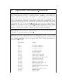
3.1
Interactive Console Mode
The Planet Simulator is started from a console by simply typing
puma.x
The following files have to be present in the same directory:
puma_namelist
land_namelist
sea_namelist
ice_namelist
ocean_namelist
surface_parameter
ocean_parameter
All settings, like length of the integration, special parameterizations etc. are given in the
namelist files. The parameter files contain the climatology. When the integration is finished
successfully, the following files have been created:
puma_output
puma_restart
land_restart
sea_restart
The file puma_output contains the model results and has to be postprocessed using the pumaburner (cf. Chapter ??). The _restart files contain information necessary to restart the
model run from the end of the current integration.
41
42
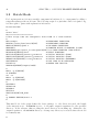
3.2
CHAPTER 3. RUNNING PLANET SIMULATOR
Batch Mode
For long integrations, it is more useful to run puma in batch mode, i.e. start puma by calling a
script that manages the model run. The following script does just that. Since it is quite long,
it is here split to parts with explanations inbetween.
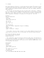
#!/usr/bin/ksh
#
stime=‘date‘
#=========================
# This script runs the atmospheric model PUMA on a linux machine
#
EXP=example
# EXPERIMENT IDENTIFIER
EXPDIR=/castor/home/user/${EXP}
# EXPERIMENT DIRECTORY
MODEL=${EXPDIR}/puma.x
# THE MODEL EXECUTABLE
SCHAUER=1
# TRANSFER OUTPUT TO SCHAUER (1=YES)
SCHAUERDIR=/pf/u/user_account/puma/${EXP} # U-TREE DIRECTORY (FOR OUTPUT)
DATADIR=${EXPDIR}/data
# OUTPUT DIRECTORY
SSTFILE=${EXPDIR}/surface_parameter
# INITIAL DATAFILE (PUMA)
SURFFILE=${EXPDIR}/surface_parameter
# INITIAL DATAFILE (PUMA)
OCEANFILE=${EXPDIR}/ocean_parameter
# INITIAL DATAFILE (OCEANMOD)
LASTYEAR=50
# LAST YEAR TO BE SIMULATED
FTPINT=12
# MONTHS PER TAR-FILE
TMPDIR=${MFHOME}/tmpdir/run$$
#
mkdir -p ${TMPDIR}
cd $TMPDIR
set -ex
mkdir -p ${EXPDIR}
mkdir -p ${DATADIR}
#
OUTYEAR=1
OUTDAY=30
OUTMON=2
OUTFTP=2
TARFILE=${EXP}TAR_0101
#
cp $MODEL $EXPDIR/model.x
#
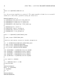
This first block of the script defines the basic settings, i.e. the directories used, the length
of the integration etc. If SCHAUER is set to 1, all puma output is transferred to the specified
directory on the schauer, thus avoiding the users directory from filling up. Otherwise, the
output is written to the DATADIR directory. A temporary directory is created where the model
is eventually run.
#
3.2. BATCH MODE
cat > $EXPDIR/NAMLIST.exe << ’EOX’
#
# NAME LIST PARAMETER
#
cat > puma_namelist << EOF
&INP
NDAYS=30,
NTSPD=32,
NRESTART=${1},
NDIAG=480,
NAFTER=32,
NEQSIG=1,
PSURF=101325.,
NPACKSP=0,
NPACKGP=0,
&END
&MISCPAR
&END
&FLUXPAR
&END
&RADPAR
&END
&RAINPAR
&END
&SURFPAR
&END
EOF
#
EOX
#
cat > ${EXPDIR}/land_namelist << EOL
&landpar
&end
EOL
cat > ${EXPDIR}/sea_namelist << EOO
&seapar
&end
EOO
cat > ${EXPDIR}/ocean_namelist << EOO
&oceanpar
&end
EOO
cat > ${EXPDIR}/ice_namelist << EOO
&icepar
&end
EOO
43
44
CHAPTER 3. RUNNING PLANET SIMULATOR
#
chmod u+x ${EXPDIR}/NAMLIST.exe
#
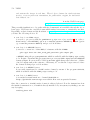
Now, the necessary namelists are generated. The puma namelist is defined as an executable
which can be called with a parameter setting the restart mode.
$EXPDIR/NAMLIST.exe 0
cp ${EXPDIR}/land_namelist land_namelist
cp ${EXPDIR}/sea_namelist sea_namelist
cp ${EXPDIR}/ice_namelist ice_namelist
cp ${EXPDIR}/ocean_namelist ocean_namelist
#
cp $EXPDIR/model.x model.x
cp ${SSTFILE} surface_parameter
cp ${SURFFILE} surface_parameter
cp ${OCEANFILE} ocean_parameter
#
model.x > ${EXPDIR}/${EXP}PROUT_0101
#
mv puma_output ${EXP}PUMA_0101
#
# history and restart saved for further diagnostics
#
tar -cf ${EXPDIR}/${TARFILE} ${EXP}PUMA_0101
mv puma_restart $EXPDIR/${EXP}RES
mv land_restart $EXPDIR/${EXP}LANDRES
mv sea_restart $EXPDIR/${EXP}SEARES
#
echo ${OUTYEAR} > ${EXPDIR}/saveyear.${EXP}
echo ${OUTDAY} > ${EXPDIR}/saveday.${EXP}
echo ${OUTMON} > ${EXPDIR}/savemon.${EXP}
echo ${OUTFTP} > ${EXPDIR}/saveftp.${EXP}
echo ${TARFILE} > ${EXPDIR}/savetar.${EXP}
#
# cat runall to EXPDIR
#
cat > $EXPDIR/runall << EOR
#!/usr/bin/ksh
#
TMPDIR=${TMPDIR}
mkdir -p \${TMPDIR}
cd \$TMPDIR
set -ex
#
EXPDIR=$EXPDIR
SCHAUER=$SCHAUER
3.2. BATCH MODE
45
SCHAUERDIR=$SCHAUERDIR
DATADIR=$DATADIR
EXP=$EXP
LASTYEAR=$LASTYEAR
MONTHS=$MONTHS
FTPINT=$FTPINT
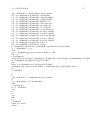
The puma namelist is generated with NRESTART=0, i.e. the first month is integrated from
climatology. The script runall is generated, which can be used to restart the run after an
interruption.
The remainder of the script is a loop of one-month integrations until the desired integration
time is reached. After each year, the monthly output is tarred together and moved to the
schauer or the data directory.
#
cp \${EXPDIR}/model.x model.x
#
##################################################################
#
II=1
while [ \$II -le 2 ]
do
#
INMON=\‘cat \${EXPDIR}/savemon.\${EXP}\‘
INYEAR=\‘cat \${EXPDIR}/saveyear.\${EXP}\‘
INDAY=\‘cat \${EXPDIR}/saveday.\${EXP}\‘
INFTP=\‘cat \${EXPDIR}/saveftp.\${EXP}\‘
TARFILE=\‘cat \${EXPDIR}/savetar.\${EXP}\‘
#
YY=\$INYEAR
if [ \${INYEAR} -lt 10 ]
then
YY=0\${YY}
fi
MM=\$INMON
if [ \${INMON} -lt 10 ]
then
MM=0\${MM}
fi
#
# make namelist
#
\$EXPDIR/NAMLIST.exe 1
cp \${EXPDIR}/land_namelist land_namelist
cp \${EXPDIR}/sea_namelist sea_namelist
cp \${EXPDIR}/ice_namelist ice_namelist
cp \${EXPDIR}/ocean_namelist ocean_namelist
46
CHAPTER 3. RUNNING PLANET SIMULATOR
#
cp \$EXPDIR/\${EXP}RES puma_restart
cp \$EXPDIR/\${EXP}LANDRES land_restart
cp \$EXPDIR/\${EXP}SEARES sea_restart
#
model.x > \${EXPDIR}/\${EXP}PROUT_\${YY}\${MM}
#
# history and restart saved for further diagnostics
#
mv puma_output \${EXP}PUMA_\${YY}\${MM}
#
if [ \${INFTP} -eq 1 ]
then
TARFILE=\${EXP}TAR_\${YY}\${MM}
echo \${TARFILE} > \${EXPDIR}/savetar.\${EXP}
tar -cf \${EXPDIR}/\${TARFILE} \${EXP}PUMA_\${YY}\${MM}
else
tar -rf \${EXPDIR}/\${TARFILE} \${EXP}PUMA_\${YY}\${MM}
fi
mv puma_restart \$EXPDIR/\${EXP}RES
mv land_restart \$EXPDIR/\${EXP}LANDRES
mv sea_restart \$EXPDIR/\${EXP}SEARES
rm \${EXP}PUMA_\${YY}\${MM}
#
OUTMON=\‘expr \${INMON} + 1\‘
OUTDAY=\‘expr \${INDAY} + 30\‘
OUTYEAR=\${INYEAR}
OUTFTP=\‘expr \${INFTP} + 1\‘
#
if [ \${OUTMON} -eq 13 ]
then
OUTMON=1
OUTYEAR=\‘expr \${OUTYEAR} + 1\‘
fi
#
echo \${OUTYEAR} > \${EXPDIR}/saveyear.\${EXP}
echo \${OUTMON} > \${EXPDIR}/savemon.\${EXP}
echo \${OUTDAY} > \${EXPDIR}/saveday.\${EXP}
#
################################################################
#
if [ \${OUTFTP} -gt \${FTPINT} ]
then
#
cd \${EXPDIR}
OUTFTP=1
3.2. BATCH MODE
47
echo \${OUTFTP} > \${EXPDIR}/saveftp.\${EXP}
tar -rf \${EXPDIR}/\${TARFILE} \${EXP}RES
tar -rf \${EXPDIR}/\${TARFILE} \${EXP}LANDRES
tar -rf \${EXPDIR}/\${TARFILE} \${EXP}SEARES
tar -rf \${EXPDIR}/\${TARFILE} NAMLIST.exe
tar -rf \${EXPDIR}/\${TARFILE} land_namelist
tar -rf \${EXPDIR}/\${TARFILE} sea_namelist
tar -rf \${EXPDIR}/\${TARFILE} ice_namelist
tar -rf \${EXPDIR}/\${TARFILE} ocean_namelist
tar -rf \${EXPDIR}/\${TARFILE} saveday.\${EXP}
tar -rf \${EXPDIR}/\${TARFILE} savemon.\${EXP}
tar -rf \${EXPDIR}/\${TARFILE} saveyear.\${EXP}
tar -rf \${EXPDIR}/\${TARFILE} savetar.\${EXP}
tar -rf \${EXPDIR}/\${TARFILE} saveftp.\${EXP}
tar -rf \${EXPDIR}/\${TARFILE} model.x
tar -rf \${EXPDIR}/\${TARFILE} runall
mv \${EXPDIR}/\${TARFILE} \${DATADIR}/\${TARFILE}to\${YY}\${MM}
if [ \${SCHAUER} -eq 1 ]
then
cat > \${EXPDIR}/put_schauer\${YY}\${MM} << EOP
set -ex
cd \${EXPDIR}
/home/larry/utils/uput2 \${DATADIR}/\${TARFILE}to\${YY}\${MM} \${SCHAUERDIR}/\${TARFI
rm \${DATADIR}/\${TARFILE}to\${YY}\${MM}
EOP
chmod u+x \${EXPDIR}/put_schauer\${YY}\${MM}
\${EXPDIR}/put_schauer\${YY}\${MM} > \${EXPDIR}/put_\${YY}\${MM} 2>&1 &
fi
cd \$TMPDIR
fi
#
echo \${OUTFTP} > \${EXPDIR}/saveftp.\${EXP}
#
if [ \${OUTYEAR} -gt \${LASTYEAR} ]
then
cd \${EXPDIR}
rm -r \${TMPDIR}
exit
fi
#
exit
EOR
#
cd $EXPDIR
chmod u+x runall
runall
48
#
etime=‘date‘
echo " "
echo "==> started, $stime"
echo " "
echo "==> done,
$etime"
echo " "
#
exit
CHAPTER 3. RUNNING PLANET SIMULATOR
Chapter 4
Parallel Program Execution
4.1
Concept
The Planet Simulator is coded for parallel execution on computers with multiple CPU’s
or networked machines. The implementation uses MPI (Message Passage Interface), that is
available for nearly every operating system http://www.mcs.anl.gov/mpi.
In order to avoid maintaining two sets of source code for the parallel and the single CPU
version, all calls to the MPI routines are encapsulated into a module. Users, that want to
compile and execute the parallel version use the module mpimod.f90 and the commands
mpif90 for compiling and mpirun for running.
If MPI is not implemented or the single CPU version is sufficient, the module mpimod dummy.f90
is used instead of mpimod.f90. Also remove or comment the line:
!
use mpi
and set the number of processors to 1:
parameter(NPRO = 1)
4.2
Parallelization in Gridpoint Domain
The data arrays in gridpoint domain are either three-dimensional e.g. gt(NLON, NLAT, NLEV)
referring to an array organized after longitudes, latitudes and levels, or two-dimensional, e.g.
gp(NLON, NLAT). The code is organized such, that there are no dependencies in latitudinal
direction, while in gridpoint domain. Such dependencies are resolved during the LegendreTransformations. So the the partitioning of the data is done in latitudes. The program can
use as many CPU’s as latitudes with the extreme of every CPU doing the computations for a
single latitude. There is the restriction however, that the number of latitudes (NLAT) divided
by the number of processors (NPRO), giving the number of latitudes per process (NLPP) must
have zero remainder. E.g. A T31 resolution uses N LAT = 48. Possible values for NPRO are
then 1, 2, 3, 4, 6, 8, 12, 16, 24, and 48.
All loops dealing with a latitudinal index look like:
do jlat = 1 , NLPP
....
enddo
49
50
CHAPTER 4. PARALLEL PROGRAM EXECUTION
There are, however, many subroutines, with the most prominent called calcgp, that can
fuse latitudinal and longitudinal indices. In all these cases the dimension NHOR is used. NHOR
is defined as: N HOR = N LON ∗ N LP P in the pumamod - module. The typical gridpoint
loop that looks like:
do jlat = 1 , NLPP
do jlon = 1 , NLON
gp(jlon,jlat) = ...
enddo
enddo
is then replaced by the faster executing loop:
do jhor = 1 , NHOR
gp(jhor) = ...
enddo
4.3
Parallelization in Spectral Domain
The number of coefficients in spectral domain (NRSP) is divided by the number of processes
(NPRO) giving the number of coefficients per process (NSPP). The number is rounded up to
the next integer and the last process may get some additional dummy elements, if there is a
remainder in the division operation.
All loops in spectral domain are organized like:
do jsp = 1 , NSPP
sp(jsp) = ...
enddo
4.4
Synchronization points
All processes must communicate and have therefore to be synchronized at following events:
• Legendre-Transformation: This involves changing from latitudinal partitioning to spectral
partitioning and such some gather and scatter operations.
• Inverse Legendre-Transformation: The partitioning changes from spectral to latitudinal
by using gather, broadcast, and scatter operations.
• Input-Output: All read and write operations must be done only by the root process, who
gathers and broadcasts or scatters the information as desired. Code that is to be executed
by the root process exclusively is written like:
if (mypid == NROOT) then
...
endif
NROOT is typically 0 in MPI implementations, mypid (My process identification) is
assigned by MPI.
4.5. SOURCE CODE
4.5
51
Source code
It needs some discipline in order to maintain parallel code. Here are the most important rules
for changing or adding code to the Planet Simulator:
• Adding namelist parameters: All namelist parameters must be broadcasted after reading
the namelist. (Subroutines mpbci, mpbcr, mpbcin, mpbcrn)
• Adding scalar variables and arrays: Global variables must be defined in a module header
and initialized.
• Initialization code: Initialization code, that contains dependencies on latitude or spectral
modes must be done by the root process only and then scattered from there to all child
processes.
• Array dimensions and loop limits: Always use parameter constants as defined in pumamod.f90
for array dimensions and loop limits.
• Testing: After significant code changes the program should be tested in single and in
multi-CPU configuration. The results of a single CPU run is usually not exactly the
same as the result of a multi-CPU run due to effects in rounding. But the results should
show only small differences during the first timesteps.
• Synchronization points The code is optimzed for parallel execution and minimizes therefore communication overhead. The necessary communication code is grouped around
the Legendre-transformations. If more scatter/gather operations or other communication routines are to be added, they should be placed just before or after the execution
of the calls to the Legendre-Transformation. Any other place would degrade the overall
performance in introducing additional process synchronization.
52
CHAPTER 4. PARALLEL PROGRAM EXECUTION
Chapter 5
Graphical User Interface
5.1
Graphical user interface (GUI)
:
The Planet Simulator may be used in the traditional fashion, with shell scripts, batch jobs,
and network queuing systems. This is acceptable for long running simulations on complex
machines and number-crunchers, like vector- computers, massive-parallel-computers and workstation clusters. There is now, however, a much more convenient method by using a graphical
user interface (GUI) for model setup with parameter configurations and for interaction between
user and model.
The Planet Simulator is configured and setup by the first GUI module named MoSt (Model
Starter, screenshot in figure NN). MoSt is the fastest way to get the model running. It gives
access to the most important parameters of the model preset to the most frequently used
values. The model can be started with a mouse click on the button labelled ”Save & Run”
either with the standard paramater setting or after editing some of the parameters in the
MoSt window. Some parameters, like horizontal and vertical resolution, or the number of
processors, require the building (compile, link and load) of new executables. MoSt achieves
this by generating and executing build scripts, that perform the necessary code changes and
create the required executable. Other parameters define startup- and boundary conditions or
settings for parameterisations. They can be edited in MoSt and, after a check for correct range
and consistency with other parameters, are written to the model’s namelist file.
Depending on all settings MoSt generates a runscript for the simulation. The user has the
choice of leaving MoSt and continue with the simulation under control of a GUI right away,
or to exit MoSt with the scripts prepared to run. The second alternative is useful for users,
who want to modify the setup beyond the scope of MoSt or want to run the Planet Simulator
without GUI.
The GUI for running the Planet Simulator (screenshot in figure NN) has two main purposes.
The first one is to display model arrays in suitable representations. Current implementations
are:
• Zonal mean cross sections
• Horizontal global fields in cylinder projection
• Horizontal global fields in polar projection
53
54
CHAPTER 5. GRAPHICAL USER INTERFACE
Figure 5.1: Screenshot of Model Starter (MoSt)
Figure 5.2: Screenshot of Graphical User Interface (GUI)
5.1. GRAPHICAL USER INTERFACE (GUI)
55
• Time-longitude (Hovmoeller) diagrams
• Time series
• Numerical values
The second purpose is the interaction part of the GUI, which allows the user to change
selected model variables during the model run. It is not necessary, though possible, to pause
the model while changing variables. Changes to model variables are, of course, monitored in
the outputfile and checked by GUI for the appropriate range of values and maximum possible
change per timestep because, otherwise, a rapid parameter change or a choice of values beyond
the normal range may blow up the model.
All model variables, which are candidates for the display or interactive changes, have a
special code to communicate with the Planet Simulator. The experienced modeller can add
new code for more variables using the existing communication code as template. Thus all model
fields or even fields received via coupling with other models can be put on the GUI display.
Both, MoSt and GUI are implemented using the Xlib (X11R5), which is a library of routines
for graphics and event communication. As this library is part of every UNIX/Linux operating
system and base of all desktop environments, there is no need to install additional software for
running MoSt and GUI. Another important property of Xlib is the full network transparency.
The display of MoSt and GUI is not locked to the machine running the programs or the model.
In fact, the best performance is obtained in running the Planet Simulator on two or four
CPUs of a remote server while displaying the GUI on the user’s workstation. In summarizing,
the MoSt and GUI programs automate many tedious tasks, minimize the time to become
familiar with the Planet Simulator, and make debugging and parameter tuning much easier.
More kinds of presentations, coordinate projections and interactivity are being developed. A
graphical preprocessor with editor for boundary conditions and a graphical postprocessor are
future expansions to build an almost complete environment for modellers.
56
CHAPTER 5. GRAPHICAL USER INTERFACE
Chapter 6
Postprocessor Pumaburner
6.1
Introduction
The Pumaburner is a postprocessor for the Planet Simulator and the PUMA model
family. It’s the only interface between raw model data output and diagnostics, graphics, and
user software.
The output data of the Planet Simulator are stored as packed binary (16 bit) values using
the model representation. Prognostic variables like temperature, divergence, vorticity, pressure,
and humidity are stored as coefficients of spherical harmonics on σ levels. Variables like radiation, precipitation, evaporation, clouds, and other fields of the parameterization package are
stored on Gaussian grids.
The tasks of the Pumaburner are:
• Unpack the raw data to full real representation.
• Transform variables from the model’s representation to a user selectable format, e.g. grids,
zonal mean cross sections, fourier coefficients.
• Calculate diagnostic variables, like vertical velocity, geopotential height, wind components, etc.
• Transfrom variables from σ levels to user selectable pressure levels.
• Compute monthly means and standard deviations.
• Write selected data either in SERVICE, GRIB, or NetCDF format for further processing.
6.2
Usage
pumaburn4 [options] InputFile OutputFile <namelist >printout
option -h : help (this output)
option -c : print available codes and names
option -d : debug mode (verbose output)
option -g : Grib
output (override namelist option)
option -n : NetCDF output (override namelist option)
57
58
CHAPTER 6. POSTPROCESSOR PUMABURNER
option -m
InputFile
OutputFile
namelist
printout
6.3
:
:
:
:
:
Mean=1 output (override namelist option)
Planet Simulator or PUMA data file
GRIB, SERVICE, or NetCDF format file
redirected <stdin>
redirected <stdout>
Namelist
The namelist values control the selection, coordinate system and output format of the postprocessed variables. Names and values are not case sensitive. You can assign values to the
following names:
Name
Def. Type Description
Example
HTYPE
S
char Horizontal type
HTYPE=G
VTYPE
S
char Vertical type
VTYPE=P
MODLEV
0
int
Model levels
MODLEV=2,3,4
hPa
0
real
Pressure levels
hPa=500,1000
CODE
0
int
ECMWF field code
CODE=130,152
GRIB
0
int
GRIB output selector
GRIB=1
NETCDF
0
int
NetCDF output selector
NETCDF=1
MEAN
1
int
Compute monthly means
MEAN=0
HHMM
1
int
Time format in Service format HHMM=0
HEAD7
0
int
User parameter
HEAD7=0815
MARS
0
int
Use constants for planet Mars MARS=1
MULTI
0
int
Process multiple input files
MULTI=12
6.4
HTYPE
HTYPE accepts the first character of the following string. Following settings are equivalent:
HTYPE = S, HTYPE=Spherical Harmonics HTYPE = Something. Blanks and the equal-sign
are optional.
Possible Values are:
Setting
Description
Dimension for T21 resolution
HTYPE = S Spherical Harmonics (506):(22 * 23 coefficients)
HTYPE = F Fourier Coefficients
(32,42):(latitudes,wavenumber)
HTYPE = Z Zonal Means
(32,levels):(latitudes,levels)
HTYPE = G Gauss Grid
(64,32):(longitudes,latitudes)
6.5
VTYPE
VTYPE accepts the first character of the following string. Following settings are equivalent:
VTYPE = S, VTYPE=Sigma VTYPE = Super. Blanks and the equal-sign are optional.
Possible Values are:
Setting
Description
Remark
VTYPE = S Sigma (model) levels Some derived variables are not available
VTYPE = P Pressure levels
Interpolation to pressure levels
6.6. MODLEV
6.6
59
MODLEV
MODLEV is used in combination with VTYPE = S. If VTYPE is not set to Sigma, the
contents of MODLEV are ignored. MODLEV is an integer array that can get as many values
as there are levels in the model output. The levels are numbered from top of the atmosphere to the bottom. The number of levels and the corresponding sigma values are listed in
the pumaburner printout. The outputfile orders the level according to the MODLEV values.
MODLEV=1,2,3,4,5 produces an output file of five model levels sorted from top to bottom,
while MODLEV=5,4,3,2,1 sorts them from bottom to top.
6.7
hPa
hPa is used in combination with VTYPE = P. If VTYPE is not set to Pressure, the contents
of hPa are ignored. hPa is a real array that accepts pressure values with the units hectoPascal
or millibar. All output variables will be interpolated to the selected pressure levels. There
is no extrapolation on the top of the atmosphere. For pressure values, that are lower than
that of the model’s top level, the top level value of the variable is taken. The variables temperature and geopotential height are extrapolated if the selected pressure is higher than the
surface pressure. All other variables are set to the value of the lowest mode level for this
case. The outputfile contains the levels in the same order as set in hPa. Example: hpa =
100,300,500,700,850,900,1000.
6.8
MEAN
MEAN can be used to compute montly means and/or deviations. The Pumaburner reads date
and time information from the model file and handles different lengths of months and output
intervals correctly.
Setting
Description
MEAN = 0 Do no averaging - all terms are processed.
MEAN = 1 Compute and write monthly mean fields. Not for spherical harmonics, Fourier coefficients or zonal means on sigma levels.
MEAN = 2 Compute and write monthly deviations. Not for spherical harmonics, Fourier coefficients or zonal means on sigma levels. Deviations
are not available for NetCDF output.
MEAN = 3 Combination of MEAN=1 and MEAN=2. Each mean field is followed by a deviation field with an identical header record. Not for
spherical harmonics, Fourier coefficients or zonal means on sigma
levels.
6.9
Format of output data
The pumaburner supports three different output formats:
• GRIB (GRIdded Binary) WMO standard for gridded data.
60
CHAPTER 6. POSTPROCESSOR PUMABURNER
• NetCDF (Network Common Data Format)
• Service Format for user readable data (see below).
For more detailed descriptions see for example:
http://www.nws.noaa.gov/om/ord/iob/NOAAPORT/resources/
Setting
Description
GRIB = 1 NetCDF = 0 The output file is written GRIB format. This option
can be used only for HTYPE=Spherical Harmonics or
HTYPE=Gauss Grid.
GRIB = 0 NetCDF = 1 The output file is written in NetCDF format. This option can be used for HTYPE=Gauss Grid only.
GRIB = 0 NetCDF = 0 The output file is written in Service format. This is
the preferred format for user programs. For a detailed
description see the following section.
GRIB = 1 NetCDF = 1 Illegal combination.
6.10
SERVICE format
The SERVICE format uses the following structure: The whole file consists of pairs of header
records and data records. The header record is an integer array of 8 elements.
head(1)
head(2)
head(3)
head(4)
head(5)
head(6)
head(7)
head(8)
=
=
=
=
=
=
=
=
ECMWF field code
modellevel or pressure in [Pa]
date [yymmdd] (yymm00 for monthly means)
time [hhmm] or [hh] for HHMM=0
1. dimension of data array
2. dimension of data array
may be set with the parameter HEAD7
experiment number (extracted from filename)
Example for reading the SERVICE format (GRIB=0 , NETCDF=0)
INTEGER HEAD(8)
REAL
FIELD(64,32)
! dimensions for T21 grids
READ (10,ERR=888,END=999) HEAD
READ (10,ERR=888,END=999) FIELD
....
888 STOP ’I/O ERR’
999 STOP ’EOF’
....
6.11
HHMM
Setting
Description
HHMM = 0 head(4) shows the time in hours (HH).
HHMM = 1 head(4) shows the time in hours and minutes (HHMM).
6.12. HEAD7
6.12
61
HEAD7
The 7th. element of the header is reserved for the user. It may be used for experiment numbers,
flags or anything else. Setting HEAD7 to a number exports this number to every header record
in the output file (SERVICE format only).
6.13
MARS
This parameter is used for processing simulations of the Mars atmosphere. Setting MARS=1
switches gravity, gas constant and planet radius to the correct values for the planet Mars.
6.14
MULTI
The parameter MULTI can bes used to process a series of input data within one run of the
pumaburner. Setting MULTI to a number (n) tells the pumaburner to procees (n) input files.
The input files must follow one of the following two rules:
• YYMM rule: The last four characters of the filename contain the data in the form YYMM.
• .NNN rule: The last four characters of the filename consist of a dot followed ny a 3-digit
sequence number.
Examples:
Namelist contains MULTI=3
Command: pumaburn <namelist >printout run.005 out
pumaburn processes the files <run.005> <run.006> <run.007>
Namelist contains MULTI=4
Command: pumaburn <namelist >printout exp0211 out
pumaburn processes the files <exp0211> <exp0212> <exp0301> <exp0302>
6.15
Namelist example
VTYPE
HTYPE
CODE
hPa
MEAN
GRIB
NETCDF
=
=
=
=
=
=
=
Pressure
Grid
130,131,132
200,500,700,850,1000
0
0
0
This namelist will write Temperature(130), u(130) and v(131) on pressure levels 200hPa,
500hPa, 700hPa, 850hPa and 1000hPa. The output interval is the same as found on the model
data, e.g. every 12 or every 6 hours (MEAN=0). The output format is SERVICE format.
62
CHAPTER 6. POSTPROCESSOR PUMABURNER
6.16
Troubleshooting
If the pumaburner reports an error or doesn’t produce the expected results, try the following:
• Check your namelist, especially for invalid codes, types and levels.
• Run the pumaburner in debug-mode by using the option -d. Example:
pumaburn <namelist >printout -d data.in data.out
This will print out some details like parameters and memory allocation during the run.
The additional information may help to detect the problem.
• Not all combinations of HTYPE, VTYPE, and CODE are valid. Try to use HTYPE=Grid
and VTYPE=Pressure before switching to exotic parameter combinations.
Chapter 7
Graphics
7.1
Grads
In this section, visualisation using the graphics package GrADS is described. A useful Internet
site for reference and installation instructions is
<http://grads.iges.org/grads/grads.html>.
Latest versions of GrADS can handle data in NETCDF format (via the command sdfopen), GRIB,
HDF-SDS, and in its native binary format. The native format can conveniently be derived from
SERVICE format. In the following it is assumed that the PUMA output has been converted to
SERVICE format with the pumaburner and the resulting file is called puma.srv. Monthly mean
data is either obtained directly from the pumaburner (namelist parameter MEAN=1, see section
6) or via a PINGO command:
srv monmeans puma.srv puma_m.srv
Information on the PINGO package can be found in DKRZ report 11 at
<http://www.mad.zmaw.de/Pingo/repdl.html>.
The SERVICE file has to be converted to GrADS’s native format by the command:
srv2gra puma_m.srv
which results in the files puma_m.gra and puma_m.ctl. The first file contains the data, the
latter one information on the grid, time steps, and variable names. The program srv2gra is
one of the postprocessing tools available at
<http://puma.dkrz.de/puma/download/map/>.
If you chose to compile it yourself, please read the comments in the first few lines of the program
text. Sometimes the srv2gra tool has difficulties to calculate an appropriate time increment
from the date headers of the data records, so you should check this. In this example the file
puma_m.ctl should look like this:
63
64
DSET ^puma_m.gra
UNDEF 9e+09
XDEF
64 LINEAR
0.0000
5.6250
OPTIONS YREV
YDEF
32 LEVELS
-85.7606 -80.2688 -74.7445 -69.2130 -63.6786
-41.5325 -35.9951 -30.4576 -24.9199 -19.3822
2.7689
8.3067
13.8445
19.3822
24.9199
47.0696
52.6065
58.1430
63.6786
69.2130
ZDEF 1 LINEAR 1 1
TDEF 12 LINEAR 00:00Z01jan0001
1mo
VARS 3
c139
0 99
139
0
0
c151
0 99
151
0
0
c175
0 99
175
0
0
ENDVARS
CHAPTER 7. GRAPHICS
-58.1430
-13.8445
30.4576
74.7445
-52.6065
-8.3067
35.9951
80.2688
-47.0696
-2.7689
41.5325
85.7606
Here, the line starting with TDEF ends with 1mo, since we are handling monthly mean data.
When the PUMA output is used without averaging, this should correspond to the output interval
given by the nafter variable used in the namelist of your PUMA run (see section ??). The
number of variables depends on how the pumaburner was called. In this example, only 3
variables were processed, i.e. the surface temperature (c139), the sea level pressure (c151) and
the albedo (c175; refer to appendix ?? for a list of codes).
The GrADS program is started by typing grads in a terminal window. Then, data is visualised
either by typing commands line-by-line, or, preferably, by using scripts. The following script,
called tglob.gs, displays the monthly mean surface temperature:
# tglob.gs
function pass(m)
’reinit’
’open puma_m’
’enable print print.mf’
’set t ’m
’c’
’set gxout shaded’
’d (c139-273.16)’
’cbar.gs’
’set gxout contour’
’d (c139-273.16)’
’draw title Surface Temperature (deg C) month ’m
’print’
’disable print’
’!gxps -i print.mf -o tglob’m’.ps’
The variable m at the beginning of the script defines the month which should be displayed. It
is passed from the terminal with the script call. Note that in this line, no quotation marks are
present, since only GrADS specific commands are framed by quotation marks. Script commands,
7.1. GRADS
65
like variable definitions, if-clauses etc. are used without quotation marks. The script is executed
by typing its name without the ending and the number of the month to be shown. For example,
tglob 7 displays the monthly mean surface temperature in July. The resulting output file is
called tglob7.ps.
The following script thh displays the time dependent surface temperature of Hamburg.
Here, two variables are passed to GrADS, the first and last day to plot (note that here, the file
puma.gra is opened, which contains data on a daily basis). The call thh 91 180 displays the
surface temperature of Hamburg for the spring season from April 1st to June 30th.
# thh.gs
function pass(d1 d2)
’reinit’
’open puma’
’enable print print.mf’
’set lat 53’
’set lon 10’
’set t ’d1’ ’d2
’c’
’d (c139-273.16)’
’draw title Surface Temperature (deg C) in Hamburg’
’print’
’disable print’
’!gxps -i print.mf -o thh.ps’
It is possible to have more than one figure in a plot, which is illustrated in the following
script. It plots seasonal means of the sea level pressure. The data file is prepared like this:
srv selcode,151 puma.srv slp.srv
srv seasmean slp.srv slp_sm.srv
srv2gra slp_sm.srv
The commands set vpage sets virtual pages inside the graphic window. The full window is
11 inch wide and 8.5 inch high, so set vpage 0 5.5 4.25 8.5 defines the upper left corner. If
setlevs=1 is specified, the pressure levels as given are used. Otherwise, GrADS defines contour
levels depending on the data set.
# slp_sm.gs
setlevs=1
’reinit’
’open slp_sm’
’enable print print.mf’
’c’
’set vpage 0 5.5 4.25 8.5’
’set gxout contour’
if (setlevs=1)
’set clevs 990 995 1000 1005 1010 1015 1020’
66
CHAPTER 7. GRAPHICS
endif
’set ccols 1’
’set grads off’
’set t 1’
’d c151/100’
’draw title SLP [hPa] yr ’ny’ DJF’
’set vpage 5.5 11 4.25 8.5’
’set gxout contour’
if (setlevs=1)
’set clevs 990 995 1000 1005 1010 1015 1020’
endif
’set ccols 1’
’set grads off’
’set t 2’
’d c151/100’
’draw title yr ’ny’ MAM’
’set vpage 0 5.5 0 4.25’
’set gxout contour’
if (setlevs=1)
’set clevs 990 995 1000 1005 1010 1015 1020’
endif
’set ccols 1’
’set grads off’
’set t 3’
’d c151/100’
’draw title yr ’ny’ JJA’
’set vpage 5.5 11 0 4.25’
’set gxout contour’
if (setlevs=1)
’set clevs 990 995 1000 1005 1010 1015 1020’
endif
’set ccols 1’
’set grads off’
’set t 4’
’d c151/100’
’draw title yr ’ny’ SON’
’print’
’disable print’
’!gxps -c -i print.mf -o slp_sm.ps’
7.2
Vis5D
“Vis5D is a system for interactive visualization of large 5-D gridded data sets such
as those produced by numerical weather models. One can make isosurfaces, contour
line slices, colored slices, volume renderings, etc of data in a 3-D grid, then rotate
7.2. VIS5D
67
and animate the images in real time. There’s also a feature for wind trajectory
tracing, a way to make text annotations for publications, support for interactive
data analysis, etc.”
from the Vis5D home page,
http://www.ssec.wisc.edu/~billh/vis5d.html
This powerful visualisation tool together with its documentation is available through the above
home page. Vis5D uses its own data format which makes it necessary to transform your data.
Depending on their format and the flowchart on http://puma.dkrz.de/puma/download/map/
you have the following choices: If
• your data is raw PUMA output,
you need to process it with the pumaburner postprocessor (see section 6) in order to
transform it to either NETCDF (option -n or namelist parameter NETCDF=1) or GRIB (option
-g or namelist parameter GRIB=1) and proceed from there.
• your data is in SERVICE format,
you need to convert it to either GRIB, for instance with the PINGOs:
grb copy2 data.srv data_with_grib_metainfo.grb output.grb,
or NETCDF, using the program puma2cdf, which is available with the PUMA postprocessing
tools. Despite of its name this program cannot process raw PUMA output but takes SERVICE
format as input. It can as well be called as srv2cdf which changes its behaviour: oddities
of model output such as the existence of February, 30th are then no longer removed. Once
the format is changed proceed from there.
• your data is in NETCDF format,
it can easily transformed to Vis5D’s native format by means of the program cdf2v2d,
which is available with the PUMA postprocessing tools.
• your data is in GRIB format,
you can find a transformation tool named Grib2V5d at
<http://grib2v5d.sourceforge.net> which offers various practical features.
Once the conversion to Vis5D’s native format is achieved please follow the instructions from
the Vis5D documentation or, if Vis5D is already installed on your system, try finding your own
way by typing:
vis5d my_data.v5d
68
CHAPTER 7. GRAPHICS
69
70
APPENDIX A. LIST OF CONSTANTS AND SYMBOLS
Appendix A
List of Constants and Symbols
A.0.1
List of Constants and Symbols
Symbol
Definition
Value
Unit
a
A
A
AS
B(T )
cc
Cchar
Ch
Cm
cp
cpd
cpv
cpi
cps
cpw
cw
Cw
D
E
E0
f
Fp
Fq
Fq
FT
Fu
Fv
F LW
F SW
g
hmix
hmixc
Hq
Hp
Jq
earth radius
= D + V~ · ∇ ln ps
absorptivity/emissivity
surface emissivity
Planck function
cloud cover
Charnock constant
transfer coefficient for heat
drag coefficient for momentum
specific heat of moist air at constant pressure
specific heat of dry air at constant pressure
specific heat of water vapor at constant pressure
specific heat of sea ice
specific heat of snow
specific heat of sea water
coefficient for the deep ocean heat flux
wetness factor
scaled divergence
evaporation
extrateristical solar flux density
Coriolis parameter =: 2Ω sin ϕ
1
tendency of the first moment=: dR
dt
0
tendency of the zeroth moment=: dR
dt
surface moisture flux
surface sensible heat flux
surface zonal wind stress
surface meridional wind stress
long wave radiation flux density
short wave radiation flux density
gravitational acceleration
mixed layer depth
climatological mixed layer depth
0
effective mixed layer depth =: TmixR−T
ref
1
reduced center of gravity =: R
R0
vertical turbulent moisture flux
6371·103
m
−
−
−
Wm−2
−
−
−
−
J kg−1 K−1
J kg−1 K−1
J kg−1 K−1
W s kg−1 K−1
W s kg−1 K−1
W s kg−1 K−1
W m−2 K−1
−
−
m s−1
W m−2
s−1
K m2 s−1
K m s−1
kg m−2 s−1
W m−2
Pa
Pa
Wm−2
Wm−2
m−2
m
m
m
m
kg m−2 s−1
0.018
1005.46
1869.46
2070
2090
4180
4
9.81
71
Lf
lh
lm
Ls
Lv
Pc
Pl
Pnm (µ)
p
pS
ps
q
Q
˜
Q
Qa
Qc
Qf
Qg
Qm
Qo
qS
qsat
R
RS
Rd
Rl
Rs
Rv
R0
R1
Ri
Sw
t
t
T
T
T0
Td
Ti
Tf
Ts
Tsea
Tmelt
Tmix
Tmixc
Tref
latent heat of fusion = Ls − Lv
mixing length for heat
mixing length for momentum
latent heat of sublimation
latent heat of vapourization
convective precipitation
large scale precipitation
associated Legendre function of the first kind
pressure
surface pressure
scaled surface pressure
specific humidity
total heat flux through sea ice
flux correction heat flux through sea ice
total atmospheric heat flux
conductive heat flux through sea ice
heat flux available for freezing sea ice
heat flux into the soil
snow melt heat flux
oceanic heat flux
surface specific humidity
saturation specific humidity
refexivity/albedo
surface albedo
gas constant for dry air
surface long wave radiation
surface short wave radiation
gas constant for water vapor
zeroth moment of the temperature distribution
first moment of the temperature distribution
Richardson number
salinity of sea water
time
scaled time step
transmissivity
temperature
temperature anomaly =: T − T0
deep ocean temperature (at 400m)
sea ice surface temperature
freezing temperature
surface temperature
sea surface temperature
melting point
mixed layer temperature
climatological mixed layer temperature
asymptotic reference temperature
3.28·105
2.8345·106
2.5008·106
287.05
461.51
34.7
271.25
273.16
J kg−1
m
m
J kg−1
J kg−1
ms−1
ms−1
−
Pa
Pa
−
kg kg−1
W m−2
W m−2
W m−2
W m−2
W m−2
Wm−2
Wm−2
W m−2
kg kg−1
kg kg−1
−
−
J kg−1 K−1
W m−2
W m−2
J kg−1 K−1
Km
K m2
−
psu
s
−
−
K
−
K
K
K
K
K
K
K
K
K
72
APPENDIX A. LIST OF CONSTANTS AND SYMBOLS
Tw
T0
U
u
u∗
V
v
~v
WL
Wsnow
Wsoil
z
z0
∆t
∆z
α
β
βd
ζ
θ
κ
κ
¯
κi
κs
λh
λm
λ
µ
µ0
ρ
ρi
ρs
ρw
ρo
σ
σ˙
σSB
τN
τF
τR
τT
τh
φ
φ
ϕ
χ
oceanic temperature profile
reference temperature profile
scaled zonal wind =: u · cos ϕ
zonal wind
friction velocity
scaled meridional wind =: v · cos ϕ
meridional wind
horizontal wind vector
cloud liquid water path
mass of snow water
soil water
height
roughness length
time increment
height increment
dρ
thermal expansion coefficient ρ1 dT
back scattering coefficient
diffusivity factor
scaled vorticity
potential temperature
Rd /Cpd
mean heat conductivity in ice and snow
heat conductivity in ice
heat conductivity in snow
asymptotic mixing length for heat
asymptotic mixing length for momentum
longitude
sin ϕ
cosine of the solar zenith angle
density of air
density of sea ice
density of snow
density of sea water
density of fresh water
normalized pressure coordinate =: p/ps
vertical velocity in σ system
Stefan-Bolzmann constant
cloud optical depth
time scale for RF
time scale for NC
time scale for temperature flux correction
time scale for depth flux correction
geopotential height := g · z
scaled geopotential height
latitude
scaled velocity potential
250.0
2.41·10−4
1.66
2.03
0.31
920
330
1030
1000
5.67·10−8
K
K
−
m s−1
m s−1
−
m s−1
m s−1
gm2
kg
m
m
m
s
m
K−1
−
−
−
K
−
W m−1 K−1
W m−1 K−1
W m−1 K−1
m
m
−
−
−
kg m−3
kg m−3
kg m−3
kg m−3
kg m−3
−
−
Wm−2 K−4
−
−
−
s
s
m2 s−2
−
−
−
73
ψ
Ω
ω˜0
scaled streamfunction
angular velocity of the earth
single scattering albedo
−5
7.292·10
−
s−1
−
74
APPENDIX A. LIST OF CONSTANTS AND SYMBOLS
Appendix B
Puma Codes
75
76
APPENDIX B. PUMA CODES
Codes available from PUMA-burner (adapted from ECHAM)
Code
110
129
130
131
132
133
135
138
139
140
141
142
143
144
146
147
148
149
151
152
153
155
156
157
159
160
Levels
1
1
NLEV
NLEV
NLEV
NLEV
NLEV
NLEV
1
1
1
1
1
1
1
1
NLEV
NLEV
1
1
NLEV
NLEV
NLEV
NLEV
1
1
Type
g
s
s
c
c
s
c
s
g
g
g
ga
ga
ga
ga
ga
c
c
c
s
g
s
c
c
g
ga
Variable
mixed layer depth
surface geopotential
temperature
u-velocity
v-velocity
specific humidity
vertical velocity
vorticity
surface temperature
soil wetness
snow depth (water equi.)
large scale precipitation
convective precipitation
snow fall
surface sensible heat flux
surface latent heat flux
horizontal streamfunktion
velocity potential
mean sea level pressure
ln(surface pressure)
cloud liquid water content
divergence
geopotential height
relative humidity
(u? )3
surface runoff
Unit
m
m2 /s2
K
m/s
m/s
kg/kg
Pa/s
1/s
K
m
m
m/s
m/s
m/s
W/m2
W/m2
m2 /s
m2 /s
Pa
kg/kg
1/s
gpm
frac.
(m/s)3
m/s
77
Code
162
164
169
170
172
173
175
176
177
178
179
180
181
182
183
203
204
205
207
208
209
210
211
212
218
221
230
232
Levels
NLEV
1
1
1
1
1
1
1
1
1
1
1
1
1
1
1
1
1
1
1
1
1
1
1
1
1
1
1
Type
g
ga
ga
g
g
g
g
ga
ga
ga
ga
ga
ga
ga
g
ga
ga
ga
g
g
g
g
g
g
g
g
ga
g
Variable
Unit
cloud cover
frac.
total cloud cover
frac.
surface temperature
K
deep soil temperature
K
land sea mask
[0:sea,1:land]
surface roughness
m
surface albedo
frac.
surface solar radiation
W/m2
surface thermal radiation
W/m2
top solar radiation
W/m2
top thermal radiation
W/m2
u-stress
Pa
v-stress
Pa
evaporation
m/s
soil temperature
K
top solar radiation upward
W/m2
surface solar radiation upward
W/m2
surface thermal radiation upward W/m2
soil temperature (level 2)
K
soil temperature (level 3)
K
soil temperature (level 4)
K
sea ice cover
frac.
sea ice thickness
m
vegetation cover
frac.
snow melt (water equiv.)
m/s
snow depth change (water equiv.) m/s
vertical integrated spec. hum.
kg/m2
glacier cover
frac.
s: PUMA spectral field; g: PUMA grid point field; c: computed by PUMA-burner; a: accumulated
78
APPENDIX B. PUMA CODES
Appendix C
Namelist
79
80
APPENDIX C. NAMELIST
basic namelist parameters
Name
Def.
Type
kick
1
int
nafter
ncoeff
ndiag
nexp
nkits
nrestart
nrun
nstep
nstop
ntspd
nrad
nflux
neqsig
nprint
nprhor
npacksp
npackgp
ndiaggp
ndiagsp
ndiagcf
ndiaggp2d
ndiaggp3d
ndiagsp2d
ndiagsp3d
nhdiff
ndel
ndl(NLEV)
ntime
nperpetual
tfrc(NLEV)
dtns
dtep
dttrp
dttrp
dtrop
psurf
tdissd
tdissz
tdisst
tdissq
tgr
time0
restim(NLEV)
t0(NLEV)
12
0
12
0
3
0
0
0
0
24
1
1
1
0
0
1
1
0
0
0
0
0
0
0
15
NLEV*2
NLEV*0
0
0
0,0,0,.. ,1
0
0.0
int
int
int
int
int
int
int
int
int
int
int
int
int
int
int
int
int
int
int
int
int
int
int
int
int
int
int
int
int
int
int
real
2.0
real
12000.0
101325.0
0.2
1.1
5.6
5.6
288.0
0.0
NLEV*15.0
NLEV*250.
real
real
real
real
real
real
real
real
real
real
Description
0: no noise initialization (ps = const.)
1: random white noise
2: Equator symmetric random white noise
3: mode (1,2) no random initialization
output interval for data [timesteps]
number of coefficients to print in wrspam
output interval for diagnostics [timesteps]
experiment identifier
number of short initial timesteps
1: preform a restart run
number of timesteps to run (excl. initial ones)
current timestep
stop at time step nstop
number of timesteps per day
1: switches radiation on
1: switches vertical diffusion on
1: use equidistant sigma levels
1: comprehensive print out (only for checks!)
1: grid point for print out (only for checks!)
1: pack spectral fields on output
1: pack gridpoint fields on output
1: process franks gp-diagnostic arrays
1: process franks sp-diagnostic arrays
1: turn on cloud forcing diagnostic
number of additional 2-d gp-diagnostic arrays
number of additional 3-d gp-diagnostic arrays
number of additional 2-d sp-diagnostic arrays
number of additional 3-d sp-diagnostic arrays
critical wavenumber for horizontal diffusion
order of hyperdiffusion for each level (2*h)
1: activate spectral printouts for this level
1: turn on time use diagnostics
radiation day for perpetual integration
Rayleigh friction timescale τF in days for each level
Pole to Pole temperature difference at surface for TR
Equator - Pole temperature difference at surface for TR
can simulate winter/summer hemispheres
a temperature increment which controls the sharpness
of the tropopause in TR
height of tropopause [m]
global mean surface pressure [Pa]
diffusion time scale for divergence [days]
diffusion time scale for vorticity [days]
diffusion time scale for temperature [days]
diffusion time scale for specific humidity [days]
global mean temperature of ground used to set TR
start time (for performance estimates)
restoration timescale for each level
reference TR -temperature profile
81
fluxmod parameters
Name
Def. Type
nevap
1
int
nshfl
1
int
nstress
1
int
nvdiff
1
int
vdiff lamm 160.0 real
vdiff b
5.0
real
vdiff c
5.0
real
vdiff d
5.0
real
Description
1: turn on surface evaporation
1: turn on surface sensible heat flux
1: turn on surface wind stress
1: turn on vertical diffusion
1: tuning parameter for vert. diff.
1: tuning parameter for vert. diff.
1: tuning parameter for vert. diff.
1: tuning parameter for vert. diff.
miscmod parameters
Name Def. Type Description
ndca
0
int
1: turn on convective adjustment
surfmod parameters
Name
Def.
nsurf
not active
noromax model resolution (NTRU)
oroscale
1.0
Type
int
int
real
seamod parameters
Name
Def.
nocean
1
nice
1
ncpl ice ocean
1
ncpl ice ocean
1
ncpl atmos ice
32
sstfile
surface parameter
albsea
0.069
albice
0.7
dz0sea
1.5 · 10−5
dz0ice
1.0 · 10−3
drhssea
1.0
drhsice
1.0
Type
int
int
int
int
int
char*80
real
real
real
real
real
real
icemod
Name
ndiag
nout
noutput
nflxcorr
parameters
Def. Type
160 int
32
int
1
int
360 int
60
int
Description
ocean model (1) or climatology (0)
sea ice model (1) or climatology (0)
ice ocean coupling time steps
ice ocean coupling time steps
atmosphere ice coupling time steps
file with sst climatology
albedo for open water
max. albedo for sea ice
roughness length sea [m]
roughness length ice [m]
wetness factor sea
wetness factor ice
Description
diagnostic output every ndiag time steps
model data output every nout time steps
1: turn on ice model output
time constant [days] for restoring
no flux correction (=0)
use flux correction from file (< 0)
oceanmod parameters
Name
Def. Type
ndiag
480 int
nout
32
int
noutput
1
int
nflxcorrmld
60
int
nflxcorrsst
Description
debug switch
resolution of orography
scaling factor for orography
Description
diagnostic output every ndiag time steps
model data output every nout time steps
1: turn on ocean model output
time constant [days] for restoring
mixed layer depth (> 0), no flux correction (=0)
use flux correction from file (< 0)
time constant [days] for restoring
sea surface temperature (> 0), no flux correction (=0)
use flux correction from file (< 0)
82
oceanmod50 parameters
Name
Def. Type Description
ndiag
480 int
diagnostic output every ndiag time steps
nout
32
int
model data output every nout time steps
noutput
1
int
1: turn on ocean model output
nflxcorrsst
-1
int
flag for calculating flux correction (< 0)
use flux correction from file (< 0)
APPENDIX C. NAMELIST