No category

Download cost733class-1.2 User guide

Transcript

cost733class-1.2
User guide
Andreas Philipp1, Christoph Beck1, Pere Esteban5,6, Frank
Kreienkamp2, Thomas Krennert9, Kai Uwe Lochbihler1, Spyros
P. Lykoudis3, Krystyna Pianko-Kluczynska8, Piia Post7,
Domingo Rasilla Alvarez10, Arne Spekat2, and Florian
Streicher1
1 University
of Augsburg, Germany
and Environment Consulting Potsdam GmbH, Germany
3 Institute of Environmental Research and Sustainable Development, National Observatory of
Athens, Greece
5 Group of Climatology, University of Barcelona, Spain
6 Institut d’Estudis Andorrans (CENMA/IEA), Principality of Andorra
7 University of Tartu, Estonia
8 Institute of Meteorology and Water Management, Warsaw, Poland
9 Zentralanstalt fuer Meteorologie und Geodynamik, Vienna, Austria
10 University of Cantabria, Santander, Spain
2 Climate
13/02/2014
Contents
1 Introduction
1
2 Installation
2.1 Getting the source code . . . . . . .
2.2 Using configure and make . . . . . .
2.2.1 configure . . . . . . . . . . . .
2.2.2 make . . . . . . . . . . . . . .
2.3 Manual compilation as an alternative
2.4 Troubleshooting . . . . . . . . . . . .
2.4.1 For configure . . . . . . . . .
2.4.2 For make . . . . . . . . . . .
2.4.3 For runtime problems . . . . .
.
.
.
.
.
.
.
.
.
2
2
2
3
4
4
5
5
5
5
.
.
.
.
.
.
.
.
.
.
.
.
.
.
.
.
.
.
.
.
.
.
.
.
.
.
.
.
.
.
.
.
.
.
.
.
.
.
.
.
.
.
.
.
.
.
.
.
.
.
.
.
.
.
.
.
.
.
.
.
.
.
.
.
.
.
.
.
.
.
.
.
.
.
.
.
.
.
.
.
.
.
.
.
.
.
.
.
.
.
.
.
.
.
.
.
.
.
.
.
.
.
.
.
.
.
.
.
.
.
.
.
.
.
.
.
.
.
.
.
.
.
.
.
.
.
.
.
.
.
.
.
.
.
.
.
.
.
.
.
.
.
.
.
.
.
.
.
.
.
.
.
.
.
.
.
.
.
.
.
.
.
.
.
.
.
.
.
.
.
.
3 Getting started
3.1 Principal usage . . . . . . . . . . . . . . . .
3.2 Quick start . . . . . . . . . . . . . . . . . .
3.2.1 Creating classifications . . . . . . . .
3.2.2 Evaluating classifications . . . . . . .
3.2.3 Comparing classifications . . . . . . .
3.2.4 Assignment to existing classifications
3.2.5 Rather simple (pre)processing . . . .
3.3 Help listing . . . . . . . . . . . . . . . . . .
.
.
.
.
.
.
.
.
.
.
.
.
.
.
.
.
.
.
.
.
.
.
.
.
.
.
.
.
.
.
.
.
.
.
.
.
.
.
.
.
.
.
.
.
.
.
.
.
.
.
.
.
.
.
.
.
.
.
.
.
.
.
.
.
.
.
.
.
.
.
.
.
.
.
.
.
.
.
.
.
.
.
.
.
.
.
.
.
.
.
.
.
.
.
.
.
.
.
.
.
.
.
.
.
.
.
.
.
.
.
.
.
.
.
.
.
.
.
.
.
.
.
.
.
.
.
.
.
7
7
8
8
9
9
9
10
10
4 Data input
4.1 Foreign formats . . . . . . . . . . . . .
4.1.1 ASCII data file format . . . . .
4.1.2 COARDS NetCDF data format
4.1.3 GRIB data format . . . . . . .
4.1.4 Other data formats . . . . . . .
4.2 Self-generated formats . . . . . . . . .
4.2.1 Binary data format . . . . . . .
4.2.2 Catalog files . . . . . . . . . . .
4.2.3 Files containing class centroids
.
.
.
.
.
.
.
.
.
.
.
.
.
.
.
.
.
.
.
.
.
.
.
.
.
.
.
.
.
.
.
.
.
.
.
.
.
.
.
.
.
.
.
.
.
.
.
.
.
.
.
.
.
.
.
.
.
.
.
.
.
.
.
.
.
.
.
.
.
.
.
.
.
.
.
.
.
.
.
.
.
.
.
.
.
.
.
.
.
.
.
.
.
.
.
.
.
.
.
.
.
.
.
.
.
.
.
.
.
.
.
.
.
.
.
.
.
.
.
.
.
.
.
.
.
.
.
.
.
.
.
.
.
.
.
.
.
.
.
.
.
.
.
.
18
18
18
19
19
20
20
20
20
21
.
.
.
.
.
.
.
.
.
.
.
.
.
.
.
.
.
.
.
.
.
.
.
.
.
.
.
4.3
4.4
Specifying data input and preprocessing . . . . . . . . . . .
4.3.1 Specification flags . . . . . . . . . . . . . . . . . . . .
4.3.2 Flags for data set description . . . . . . . . . . . . .
4.3.3 Flags for spatial data Selection . . . . . . . . . . . .
4.3.4 Flags for data Preprocessing . . . . . . . . . . . . . .
4.3.5 Flags for data Postprocessing . . . . . . . . . . . . .
4.3.6 Options for selecting dates . . . . . . . . . . . . . . .
4.3.7 Using more than one data set . . . . . . . . . . . . .
4.3.8 Options for overall PCA preprocessing of all data sets
Examples . . . . . . . . . . . . . . . . . . . . . . . . . . . .
4.4.1 Simple ASCII data matrix . . . . . . . . . . . . . . .
4.4.2 ASCII data file with date columns . . . . . . . . . . .
4.4.3 NetCDF data selection . . . . . . . . . . . . . . . . .
4.4.4 Date selection for classification and centroids . . . . .
5 Data output
5.1 The classification catalog . . . . . . . .
5.2 Centroids or type composits . . . . . .
5.3 Output on the screen . . . . . . . . . .
5.4 Output of the input data . . . . . . . .
5.5 Output of indices used for classification
5.6 Opengl graphics output . . . . . . . . .
.
.
.
.
.
.
.
.
.
.
.
.
.
.
.
.
.
.
.
.
.
.
.
.
.
.
.
.
.
.
.
.
.
.
.
.
.
.
.
.
.
.
.
.
.
.
.
.
.
.
.
.
.
.
.
.
.
.
.
.
.
.
.
.
.
.
.
.
.
.
.
.
. . . . .
. . . . .
. . . . .
. . . . .
. . . . .
. . . . .
. . . . .
. . . . .
together
. . . . .
. . . . .
. . . . .
. . . . .
. . . . .
.
.
.
.
.
.
.
.
.
.
.
.
.
.
.
.
.
.
.
.
.
.
.
.
.
.
.
.
.
.
.
.
.
.
.
.
.
.
.
.
.
.
.
.
.
.
.
.
.
.
.
.
.
.
.
.
.
.
.
.
.
.
.
.
21
22
23
25
25
28
28
29
30
30
30
31
32
32
.
.
.
.
.
.
33
33
33
33
34
34
34
6 Classification methods
35
6.1 Methods using predefined types . . . . . . . . . . . . . . . . . . . . . . . 35
6.1.1 INT | interval | BIN | binclass . . . . . . . . . . . . . . . . . . . . 35
6.1.2 GWT | prototype - large scale circulation types . . . . . . . . . . 36
6.1.3 GWTWS | gwtws - large scale circulation types . . . . . . . . . . 37
6.1.4 LIT | lit - litynski threshold based method . . . . . . . . . . . . . 39
6.1.5 JCT | jenkcol - Jenkinson-Collison Types . . . . . . . . . . . . . . 42
6.1.6 WLK | wlk - automatic weather type classification according to
German metservice . . . . . . . . . . . . . . . . . . . . . . . . . . 46
6.2 Methods based on Eigenvectors . . . . . . . . . . . . . . . . . . . . . . . 49
6.2.1 PCT | tpca - t-mode principal component analysis using oblique
rotation . . . . . . . . . . . . . . . . . . . . . . . . . . . . . . . . 49
6.2.2 PTT | tpcat - t-mode principal component analysis using orthogonal rotation . . . . . . . . . . . . . . . . . . . . . . . . . . . . . 50
6.2.3 PXE | pcaxtr - the extreme score method . . . . . . . . . . . . . . 50
6.2.4 KRZ | kruiz - Kruizingas PCA-based types . . . . . . . . . . . . . 52
6.3 Methods using the leader algorithm . . . . . . . . . . . . . . . . . . . . . 54
6.3.1 LND | lund - the Lund-method . . . . . . . . . . . . . . . . . . . 54
6.3.2 KIR | kh - Kirchhofer . . . . . . . . . . . . . . . . . . . . . . . . . 55
6.4
6.5
6.6
6.3.3 ERP | erpicum . . . . . . . . . . . . . . . . . . . . . . . . . . . .
Hierarchical Cluster analysis . . . . . . . . . . . . . . . . . . . . . . . . .
6.4.1 HCL | hclust . . . . . . . . . . . . . . . . . . . . . . . . . . . . .
Optimization algorithms . . . . . . . . . . . . . . . . . . . . . . . . . . .
6.5.1 KMN | kmeans - conventional k-means with random seeds . . . .
6.5.2 CAP | pcaca - k-means of time filtered PC-scores and HCL starting
partition . . . . . . . . . . . . . . . . . . . . . . . . . . . . . . . .
6.5.3 CKM | ckmeans - k-means with dissimilar seeds . . . . . . . . . .
6.5.4 DKM | dkmeans - a variant of ckmeans . . . . . . . . . . . . . . .
6.5.5 PXK | pcaxtrkm - k-means using PXE starting partitions . . . . .
6.5.6 SAN | sandra - simulated annealing and diversified randomization
6.5.7 SAT | sandrat - time constrained simulated annealing and diversified randomization . . . . . . . . . . . . . . . . . . . . . . . . .
6.5.8 SOM | som - self organizing (feature) maps (neural network according to Kohonen) . . . . . . . . . . . . . . . . . . . . . . . . .
6.5.9 KMD | kmedoids - partitioning around medoids . . . . . . . . . .
Random classifications . . . . . . . . . . . . . . . . . . . . . . . . . . . .
6.6.1 RAN | random . . . . . . . . . . . . . . . . . . . . . . . . . . . .
6.6.2 RAC | randomcent . . . . . . . . . . . . . . . . . . . . . . . . . .
56
58
58
59
59
60
61
62
62
66
66
67
67
68
68
69
7 Assignments to existing classifications
70
7.1 ASC | assign . . . . . . . . . . . . . . . . . . . . . . . . . . . . . . . . . . 70
7.2 CNT | centroid . . . . . . . . . . . . . . . . . . . . . . . . . . . . . . . . 70
8 Evaluation of classifications
72
8.1 EVPF | evpf - explained variation and pseudo F value . . . . . . . . . . . 72
8.2 ECV | exvar . . . . . . . . . . . . . . . . . . . . . . . . . . . . . . . . . . 73
8.3 WSDCIM | wsdcim - Within-type standard deviation and confidence interval of the mean . . . . . . . . . . . . . . . . . . . . . . . . . . . . . . . 73
8.4 DRAT | drat - Ratio of distances within and between circulation types . 74
8.5 FSIL | fsil - Fast Silhouette Index . . . . . . . . . . . . . . . . . . . . . . 75
8.6 SIL | sil - Silhouette Index . . . . . . . . . . . . . . . . . . . . . . . . . . 76
8.7 BRIER | brier - Brier Score . . . . . . . . . . . . . . . . . . . . . . . . . 76
9 Comparison of classifications
78
9.1 CPART | cpart - Catalog comparison . . . . . . . . . . . . . . . . . . . . 78
10 Miscellaneous functions
79
10.1 AGG | agg - Aggregation . . . . . . . . . . . . . . . . . . . . . . . . . . . 79
10.2 COR | cor - Correlation . . . . . . . . . . . . . . . . . . . . . . . . . . . 79
10.3 SUB | substitute - Substitute . . . . . . . . . . . . . . . . . . . . . . . . 79
11 Visualization
81
12 Development
12.1 Implementing a new subroutine . . . . .
12.2 Packing the directory for shipping . . . .
12.3 Use of variables in the subroutine . . . .
12.4 Using the input data from datainput.f90
12.5 The gnu autotools files . . . . . . . . . .
82
82
84
84
85
86
References
.
.
.
.
.
.
.
.
.
.
.
.
.
.
.
.
.
.
.
.
.
.
.
.
.
.
.
.
.
.
.
.
.
.
.
.
.
.
.
.
.
.
.
.
.
.
.
.
.
.
.
.
.
.
.
.
.
.
.
.
.
.
.
.
.
.
.
.
.
.
.
.
.
.
.
.
.
.
.
.
.
.
.
.
.
.
.
.
.
.
88
1 Introduction
1
1 Introduction
cost733class is a FORTRAN software package focussed on creating and evaluating
weather and circulation type classifications utilizing various different methods. The
name refers to COST Action 733 which has been an initiative started in the year 2005
within the ESSEM (Earth System Science and Environmental Management) domain of
the COST (European Cooperation in Science and Technology) framework. The topic
of COST 733 is "Harmonisation and Applications of Weather Type Classifications for
European regions". cost733class is released under GNU General Public License v3
(GPL) and freely available.
2 Installation
2
2 Installation
The software is developed on Unix/Linux operating systems, however it may possible
to compile and run it on other operating systems too, although some features may not
work. At the time of writing this affects the NetCDF and grib data format and the
OpenGL visualisation, which are not necessary to run the program.
2.1 Getting the source code
When you read this, you might have downloaded the software package and unpacked it
already. However here is the way how to get and compile the software:
To download direct your web browser to:
h t t p : / / c o s t 7 3 3 c l a s s . geo . uni−a u g s b u r g . de / c o s t 7 3 3 c l a s s −1.2
Here you will find instructions how to download the source code by SVN or how to get
a tar package.
If you have the tar-package unpack the bzip2 compressed tar-file e.g. by:
t a r x v f j c o s t 7 3 3 c l a s s −1.2 _RC_revision ? ? . t a r . bz2
where ?? stands for the svn version number.
Change into the new directory:
cd c o s t 7 3 3 c l a s s −1.2
2.2 Using configure and make
The next step is to compile the source code to generate the executable called
cost733class. For this you need to have a C and a FORTRAN90 compiler installed
on your system. The compiler reads the source code from the src directory and generates the executable src/cost733class in the same directory which can be started on
the command line of a terminal. In order to prepare the compilation process for automatic execution, so called Makefiles are generated by a script called configure. The
configure script checks whether everything (tools, libraries, compilers) which is needed
for compilation is installed on your system. If configure stops with an error, you have
to install the package it is claiming about (see troubleshooting) and rerun configure
until it is happy and creates the Makefiles. The package include some example shell
scripts containing the command to configure and make the software in one step:
2 Installation
3
• compile_gnu_debug.sh: this script uses the GNU Linux compilers gcc, gfortran
and c++ to compile the software with NetCDF support but without opengl support. Debugging information will be given in case of software errors.
• compile_gnu_debug_opengl.sh: this script additionally includes opengl support
for visualization.
• compile_gnu_debug_grib.sh: this script additionally includes grib support.
• compile_gnu_debug_omp.sh:this script additonally includes compiler options to
run parts of the code in parallel.
• compile_intel_omp.sh: this script uses the intel compiler suite.
In order to execute these scripts you type e.g.:
. / compile_gnu_debug_opengl . sh
or
sh compile_gnu_debug_opengl . sh
These scripts can be easily copied and modified to save compiler options which are
often needed. However it is also possible to run the two commands configure and make
manually one after the other, as described in the following.
2.2.1 configure
The configure script tries to guess which compilers should be used, however it is advicable
to specifiy the compilers by setting the FC= and CC= flags. E.g. if you want to use the
GNU compilers gfortran and gcc say:
. / c o n f i g u r e FC=g f o r t r a n CC=g c c
or if the intel compilers should be used:
. / c o n f i g u r e FC= i f o r t CC=i c c
Note that the FORTRAN and C compilers should be able to work together, i.e. the
binaries must be compatible. This is not always the case e.g. when mixing other and
GNU compilers (depending on versions).
Also you can use some special compiler options, e.g. for running parts of the classifications in parallel:
. / c o n f i g u r e FC= i f o r t CC=i c c FCFLAGS="− p a r a l l e l −openmp"
In the same manner options for the C-compiler can be set by the CCFLAGS="..." option.
Further options for the configure script control special features of the package:
. / c o n f i g u r e −−d i s a b l e −n e t c d f
2 Installation
4
switches off the compilation of the NetCDF library, thus only ASCII data can be read
by the software.
. / c o n f i g u r e −−e n a b l e −g r i b −−d i s a b l e −j p e g
switches on the compilation of the GRIB_API, thus grib data can be read by the
software. This requires the "jasper" package.
. / c o n f i g u r e −−e n a b l e −o p e n g l
switches on the compilation of routines which visualise some of the classification processes like SOM, SAN or CKM. This feature is working only for unix systems with
opengl-development packages (gl-dev glut-dev x11-dev) installed.
2.2.2 make
The compiling process itself is done by the tool called make:
make
If everthing went well, you will find the excutable cost733class in the src directory.
Check it by running the command:
src / cost733class
If you have administrator priviledges on your system you can install the executables
into /usr/local/bin. Note that the NetCDF tools coming along with cost733class are
also installed there.
sudo su −
make i n s t a l l
Alternatively you can copy only the excutable to any bin directory to have it in your
command search path:
sudo copy s r c / c o s t 7 3 3 c l a s s / u s r / l o c a l / b i n
That’s it, you can now start to run classifications, which of course needs some input
data describing the atmospheric state of each time step (i.e. object) you want to classify.
You can now try with the next chapter (Quick start) or look into the Data input chapter.
2.3 Manual compilation as an alternative
Within the package directory there is a batch file called compile_mingw.bat for Windows. This script file contains the direct compile command for the gfortran and g95
compiler without any dependencies to any libraries. It can be used if no NetCDF input
is needed or if there are troubles compiling the NetCDF package.
2 Installation
5
2.4 Troubleshooting
2.4.1 For configure
• If configure claims about something missing or a wrong version number, you have
to install or update the concerning software packages. For Debian and Ubuntu
systems that’s rather easy. First you have to find out the official name of the
package which contains the files configure was claiming about. Here you can use
the tool apt-file which must be installed first, updated and run:
sudo apt−g e t i n s t a l l apt− f i l e
apt− f i l e update
apt− f i l e s e a r c h <f i l e n a m e >
It will then print the name of the package in the first column and you can use it
to install the missing package:
sudo apt−g e t i n s t a l l <package>
2.4.2 For make
• If the following error meassage appears:
C a t a s t r o p h i c e r r o r : c o u l d not s e t l o c a l e "" t o a l l o w p r o c e s s i n g o f
multibyte characters
setting the environment variable LANG to C
e x p o r t LANG=C
in the shell you use for compilation will fix it.
2.4.3 For runtime problems
• Some methods need a lot of RAM and maybe more than is available. If this is the
case you can try to enlarge stacksize each time you run the software by
u l i m i t −s u n l i m i t e d
• If the following error or a similar error occurs:
∗∗∗ g l i b c d e t e c t e d ∗∗∗ d o u b l e f r e e o r c o r r u p t i o n ( ! p r e v ) : 0 x08196948 ∗∗∗
this is probably due to differing compiler/library versions. You can try to get rid
of it by:
e x p o r t MALLOC_CHECK_=0
2 Installation
6
• If compiled with grib support and running cost733class results in the following
error:
GRIB_API ERROR
:
Unable t o f i n d boot . d e f
g r i b _ c o n t e x t . c a t l i n e 1 5 6 : a s s e r t i o n f a i l u r e A s s e r t ( 0 ) Aborted
one has to define the path to the so called grib definitions. In an Unix environment
something like
e x p o r t GRIB_DEFINITION_PATH="/PATH/ c o s t 7 3 3 c l a s s −1.2/ g r i b _ a p i − 1 . 9 . 1 8 / d e f i n i t i o n s "
should do it. Use absolute paths!
• Depending on the processor type and data size method SAN and SOM may run
for several hours up to days. This is no bug!
3 Getting started
7
3 Getting started
3.1 Principal usage
cost733class has been written to simplify and unify the generation of classification
catalogues. It’s functionality is controlled by command line arguments, i.e. options are
given as key words after the command which is entered into a terminal or console providing a command prompt. The command line interface (CLI) makes the software suitable
for shell scripts and can easily run on compute servers or clusters in the background.
Recently a graphical user interface (GUI) has been added by using the OpenGL menu
functions which is accessible by a right click into the OpenGL window, however it is not
very intuitive yet. Therefore the documentaion will concentrate on the CLI interface.
If you type src/cost733class just after the compilation process you will see the
output of the -help function. In order to run a classification, you have to provide
command line arguments for the program, i.e. you have to type expressions behind the
cost733class command which are separated by blanks (" "). The program will scan
the command line and recognize all arguments beginning with a "-", several of which
have to be followed by another expression. All expressions have to be separated by one
or more blanks, which is the reason that inbetween any expression (e.g. a file name)
no blank is allowed. Also all expressions have to be written in lower/upper case letters
if said so in the -help output. Command lines can be rather simple, however some
methods and the data configurations can be complex, thus that the command line gets
longer and longer the more you want to fine tune your classification. In this case, and
especially if just variations of a classifications should be run one after another, it can be
useful to use shell scripts to run the software which will be explained below.
In order to understand which options play a role for which part of the classification it is
helpful to distinguish between options relevant for the data input and preprocessing and
options relevant for the routines itself. In order to better understand how the software
works and how it can be used, the workflow is briefly described in the following:
In the first step the command line arguments are analysed (subroutine arguments()).
For each option default values are set within the program, however they are changed if
respective options are provided by the user. The next step is to evaluate the data which
should be read from a file, especially the size of the data set has to be determined here
in order to reserve (allocate) computer memory for it. Then the data are read into a
preliminary array (RAWDAT) and eventually are preprocessed (selected, filtered, etc.)
before they are put into the final, synchronized, DAT array which is used by the methods.
3 Getting started
8
In some cases (depending on the classification/evaluation operation) existing catalogues
have to read. This is done in the next step by the subroutine classinput(). Afterwards
the subroutine for the desired operation is called. If this subroutine finished with a new
catalogue, it is written to a classification catalogue file (*.cla) and the program ends.
Other routines e.g. for comparison or evaluation of classification catalogues might just
produce screen output.
3.2 Quick start
As an requirement to write complex commands it is necessary to understand the basic
synopsis of cost733class. There are several different use cases in which cost733class
can be used:
1. Creation of classifications of any numerical data following an entity-attribute-value
model (main purpose of cost733class). For more information about the data
model used by cost733class see section 4.
2. Evaluation of such classifications
3. Comparison of such classifications
4. Assignment of existing classifications to new data
5. Rather simple data (pre)processing
All of these use cases require different commands following different structures. Therefor
the next sections give brief instructions on how to use cost733class for each of these
five cases.
3.2.1 Creating classifications
For the creation of classfications a basic command follows the scheme:
c o s t 7 3 3 c l a s s −dat < s p e c i f i c a t i o n > [− dat < s p e c i f i c a t i o n >] −met <method> [− n c l
] [− c n t <f i l e n a m e >] [− c l a < f i l e >] [ more method s p e c i f i c o p t i o n s ]
Essential for a successful completion of each classification run is the -dat <specification>
option which provides necessary information about the input data. For some methods it
is possible to give more than one data specification option, for others it is preriquesite.
Furthermore the classification method must be named by the -met <method> option.
The number of classes can be specified with -ncl <integer>. The filenames for the output of the classfication catalog and the corresponding class centroids can be defined by
-cla <filename> and -cnt <filename>. Depending on the used classification method
several other options can be provided by special options. For further documentation of
these consult the relative section.
Based on this the command for a classification with the method KMN may look like:
3 Getting started
9
c o s t 7 3 3 c l a s s −dat pth : s l p . dat −n c l 9 −met KMN −c l a KMN_ncl9 . c l a
3.2.2 Evaluating classifications
The basic scheme of an evaluation command is:
c o s t 7 3 3 c l a s s −dat < s p e c i f i c a t i o n > [− dat < s p e c i f i c a t i o n >] − c l a i n < s p e c i f i c a t i o n > −met
<method> [− i d x <f i l e n a m e >] [ more method s p e c i f i c o p t i o n s ]
The most important difference to a classification run is the -clain <specification>
option. It defines the path to an existing classification catalog file and is mandatory
for all evaluation methods. The desired evaluation method must be chosen by the
-met <method> option. The results are written to one or more files for which the basename can be given by the -idx <filename> option. Analogous to the previous command
every method has its additional options which are explained in the corresponding sections below. At least one -dat <specification> option describes the data one wants
to evaluate with.
A cost733class run which evaluates the classification generated by the previous command using the Brier Score would be:
c o s t 7 3 3 c l a s s −dat pth : s l p . dat − c l a i n pth : KMN_ncl9 . c l a −met BRIER −i d x
brier_KMN_ncl9 . t x t
3.2.3 Comparing classifications
Comparing two or more classifications is rather easy:
c o s t 7 3 3 c l a s s − c l a i n < s p e c i f i c a t i o n > [− c l a i n < s p e c i f i c a t i o n >] −met <method> [− i d x
<f i l e n a m e >] [ more method s p e c i f i c o p t i o n s ]
The only difference to an evaluation and classification run is the absence of the
-dat <specification> option. Instead at least two classification catalogs (more than
one per file are possible) must be provided.
A comparison of two partitions based on different methods could be done with:
c o s t 7 3 3 c l a s s − c l a i n pth : DKM_ncl9 . c l a − c l a i n pth : KMN_ncl9 . c l a −met CPART −i d x
KMN_DKM_ncl9_compared . t x t
3.2.4 Assignment to existing classifications
Assignments to existing classifications can be done on two different bases:
1. for a given classification catalog
2. for predefined class centroids
3 Getting started
10
In both cases one has to provide and describe data which is then assigned to an existing
classification. Other required cost733class options differ in both cases. Please refer to
the corresponding sections below.
3.2.5 Rather simple (pre)processing
Beyond the use cases mentioned above there are a few methods in cost733class which
process input data in a different way. They are grouped together under the term miscellaneous functions.
Furthermore it is possible to just preprocess input data without calling a distinctive
method.
c o s t 7 3 3 c l a s s −dat < s p e c i f i c a t i o n > [ o p t i o n s f o r s e l e c t i n g d a t e s ] −w r i t e d a t <f i l e n a m e >
In this case data output can be accomplished by the -witedat <filename> option.
There are several flags for preprocessing and spatial selection which are listed and described in the relative section. An example might be:
c o s t 7 3 3 c l a s s −dat pth : s l p . dat l o n : − 1 0 : 3 0 : 2 . 5
lat :35:60:2.5 fdt :2000:1:1:12
l d t : 2 0 0 8 : 1 2 : 3 1 : 1 2 ddt : 1 d ano : 3 f i l : 3 0 −p e r 2 0 0 0 : 1 : 1 : 1 2 , 2 0 0 5 : 1 2 : 3 1 : 1 2 , 1 d −w r i t e d a t
ou tp ut . b i n
Note that the output data are unformatted binary files. These files can be read by
cost733class in a subsequent run. This proceeding can be very helpful if many runs
of cost733class are planned.
3.3 Help listing
If you run the cost733class command without any command line argument (or with
the -help option) you should see the following help text, giving a brief description of
the various options:
USAGE:
. . / s r c / c o s t 7 3 3 c l a s s −dat < s p e c i f i c a t i o n > [− dat < s p e c i f i c a t i o n >] [ o p t i o n s ]
OPTIONS :
____________________________________________________________________
INPUT DATA:
−dat <char>
:
:
:
:
:
:
:
:
:
:
:
s p e c i f i c a t i o n o f i n p u t data . More than one ’− dat ’ arguments
a r e a l l o w e d t o combine data o f same sample s i z e but from
d i f f e r e n t f i l e s in d i f f e r e n t formats .
<char> c o n s i s t s o f v a r i o u s s p e c i f i c a t i o n s s e p a r a t e d by t h e
c h a r a c t e r ’@’ o r one o r more b l a n k s ’ ’ :
@var:<name o f v a r i a b l e > f o r fmt : n e t c d f t h i s must be t h e
v a r i a b l e name i n t h e n e t c d f f i l e
@pth:< path f o r i n p u t data f i l e >
i n c a s e o f n e t c d f i t may i n c l u d e "?" symbols t o be
r e p l a c e d by numbers g i v e n by t h e f d t : and l d t : f l a g s .
@fmt: <" a s c i i " o r " n e t c d f " o r " g r i b "> d e f a u l t a s c i i
3 Getting started
−r e a d n c d a t e
11
:
:
:
:
:
:
:
:
:
:
:
:
:
:
:
:
:
:
:
:
:
:
:
:
:
:
:
:
:
:
:
:
:
:
:
:
:
:
:
:
:
:
:
:
:
:
:
:
:
:
:
:
:
I f f i l e name ends with " . nc " n e t c d f i s assumed ;
f o r " . g r i b / . grb / . gribX / . grbX" (X= [ 1 , 2 ] ) g r i b i s assumed .
a s c i i : ( d e f a u l t ) a s c i i f i l e with one l i n e p e r day ( o b j e c t
t o c l a s s i f y ) and one column p e r v a r i a b l e ( p a r a m e t e r
d e f i n i n g t h e o b j e c t s ) t h e columns have t o be d e l i m i t e d
by one o r more b l a n k s . The number o f o b j e c t s and
v a r i a b l e s i s s ca n ne d by t h i s program on i t s own .
n e t c d f : data i n s e l f d e s c r i b i n g n e t c d f f o r m a t .
time and g r i d i s sc an n ed a u t o m a t i c a l l y .
g r i b : data i n s e l f d e s c r i b i n g f o r m a t .
time and g r i d i s sc an n ed a u t o m a t i c a l l y .
@dtc:<1−4> ( number o f l e a d i n g d a t e columns : year , month ,
day , hour i n a s c i i f i l e )
@fdt :<YYYY:MM:DD:HH> f i r s t d a t e i n d a t a s e t ( d e s c r i p t i o n )
@ldt :<YYYY:MM:DD:HH> l a s t d a t e i n d a t a s e t ( d e s c r i p t i o n )
@ddt:<y |m| d | h> time s t e p i n data s e t i n y e a r s , months ,
days o r h o u r s
@mdt:< l i s t o f months> months i n data s e t , e . g . @mdt : 1 : 2 : 1 2
@lon:< minlon >:<maxlon >:< d i f l o n > l o n g i t u d e d e s c r i p t i o n
@lat :< m i n l a t >:<maxlat >:< d i f l a t > l a t i t u d e d e s c r i p t i o n
@slo :< minlon >:<maxlon >:< d i f l o n > l o n g i t u d e s e l e c t i o n
@sla :< m i n l a t >:<maxlat >:< d i f l a t > l a t i t u d e s e l e c t i o n
@ s l e :< l e v e l between 1000 and 10> s e l e c t i o n
@arw: a r e a w e i g h t i n g 1=c o s ( l a t i t u d e ) ,
2= s q r t ( c o s ( l a t i t u d e ) ) ,
3= c a l c u l a t e d w e i g h t s by a r e a o f g r i d box which i s t h e same
as cos ( l a t i t u d e ) of option 1
@ s c l :< f l o a t > s c a l i n g o f data v a l u e s
@ o f f :< f l o a t > o f f s e t v a l u e t o add a f t e r s c a l i n g
@nrm: o b j e c t ( row−w i s e ) n o r m a l i s a t i o n :
1= c e n t e r i n g ,2= s t d ( sample ) ,3= s t d ( p o p u l a t i o n )
@ano: v a r i a b l e ( column−w i s e ) n o r m a l i s a t i o n :
done a f t e r s e l e c t i o n o f time s t e p s :
−1=c e n t e r i n g ,−2= s t d ( sample ) ,−3= s t d ( p o p u l a t i o n )
done b e f o r e s e l e c t i o n o f time s t e p s :
1= c e n t e r i n g ,2= s t d ( sample ) ,3= s t d ( p o p u l a t i o n )
11= c e n t e r i n g f o r days o f year ,
12= s t d f o r days ( sample ) ,13= s t d ( p o p u l a t i o n )
21= c e n t e r i n g f o r months ,
22= s t d f o r months ( sample ) ,
23= s t d ( p o p u l a t i o n )
31= c e n t e r i n g on monthly mean ( r u n n i n g 31 day window ) ,
32= s t d f o r months ( sample ) ( r u n n i n g 31 day window ) ,
33= s t d ( p o p u l a t i o n ) ( r u n n i n g 31 day window )
@ f i l : g a u s s i a n time f i l t e r i n t >0 −> low−p a s s
i n t <0 −> high−p a s s
@pca:< f l o a t | i n t e g e r > PCA o f p a r a m e t e r data s e t :
i f <f l o a t >: f o r r e t a i n i n g e x p l a i n e d v a r i a n c e
f r a c t i o n , i f : number o f PCs
@pcw:< f l o a t | i n t e g e r > a s @pca but with w e i g h t i n g by
explained variance
@seq:< s e q u e n c e l e n g t h f o r e x t e n s i o n >
@wgt:< w e i g h t i n g f a c t o r >
:
:
:
:
@cnt:< f i l e name> f i l e name t o w r i t e c e n t r o i d / c o m p o s i t e
v a l u e s t o i f e x t e n s i o n = " ∗ . nc " i t i s n e t c d f format ,
a s c i i o t h e r w i s e ( with c o o r d i n a t e s f o r ∗ . t x t , w i t h o u t
f o r ∗ . dat ) .
: r e a d t h e d a t e o f o b s e r v a t i o n s from n e t c d f time v a r i a b l e r a t h e r
:
than c a l c u l a t i n g i t from " a c t u a l r a n g e " a t t r i b u t e o f t h e
:
time v a r i a b l e ( s l o w s down t h e data i n p u t but can o v e r r i d e
:
buggy a t t r i b u t e e n t r i e s a s e . g i n s l p . 2 0 1 1 . nc ) .
3 Getting started
12
−p e r <char>
: p e r i o d s e l e c t i o n , <char> i s e . g . 2 0 0 0 : 1 : 1 : 1 2 , 2 0 0 8 : 1 2 : 3 1 : 1 2 , 1 d
−mon <char>
:
:
:
l i s t o f months t o c l a s s i f y : MM,MM,MM, . . .
e . g . : −mon 1 2 , 0 1 , 0 2 c l a s s i f i e s w i n t e r data ( d e f a u l t i s
months ) , o n l y a p p l i e s i f −p e r i s d e f i n e d !
all
−mod
: LIT : s e t a l l months t o be 30 days l o n g ( r e l e v a n t f o r −met l i t )
− d l i s t <char>
:
:
:
:
:
−c a t <spe c >
:
−c n t i n <char>
: centroid input f i l e
l i s t f i l e name f o r s e l e c t i n g a s u b s e t o f d a t e s w i t h i n t h e
g i v e n p e r i o d f o r c l a s s i f i c a t i o n . Each l i n e has t o h o l d one
d a t e i n form : "YYYY MM DD HH" f o r year , month , day , hour .
I f hour , day o r month i s i r r e l e v a n t p l e a s e p r o v i d e t h e c o n s t a n t
dummy number 0 0 .
c l a s s i f i c a t i o n c a t a l o g i n p u t , where <sp ec > c o n s i s t s o f t h e f o l l o w i n g
flags :
@pth:< path f o r f i l e >
@fdt :< f i r s t date>
@ldt :< l a s t date>
@ddt:< time s t e p , e . g . "@ddt : 1 d" f o r one day>
@dtc:<number o f d a t e columns>
@mdt:< l i s t o f months> e . g . "@mdt : 0 1 , 0 2 , 1 2 "
−catname <char> : f i l e with a s many l i n e s a s c a t a l o g s r e a d i n by "− c a t " ,
each l i n e c o n t a i n s t h e name o f t h e c a t a l o g o f t h e c o r r e s o n d i n g
column i n t h e c a t a l o g f i l e .
f o r −met ASS and ASC
−pca < f l o a t | i n t e g e r >: PCA o f i n p u t data a l l t o g e t h e r :
: i f <f l o a t >: f o r r e t a i n i n g e x p l a i n e d v a r i a n c e f r a c t i o n
: i f : number o f PCs
−pcw < f l o a t | i n t e g e r >: PCA o f i n p u t data , PCs w e i g h t e d by e x p l a i n e d v a r i a n c e :
: i f <f l o a t >: f o r r e t a i n i n g e x p l a i n e d v a r i a n c e f r a c t i o n
: i f : number o f PCs
____________________________________________________________________
OUTPUT:
−c l a < c l a f i l e > : name o f c l a s s i f i c a t i o n ou tp ut f i l e ( c o n t a i n s number o f c l a s s
: f o r each o b j e c t i n one l i n e ) .
: d e f a u l t = ./ < basename ( d a t f i l e )>_<method>_ncl. c l a
−mcla < c l a f i l e >: m u l t i p l e c l a s s i f i c a t i o n ou tp ut f i l e . Some methods g e n e r a t e
: more than one (−nrun ) c l a s s i f i c a t i o n and s e l e c t t h e b e s t .
: o p t i o n −mcla < f i l e > makes them w r i t i n g out a l l .
−skipempty <F | T> : s k i p empty c l a s s e s i n t h e numbering scheme ? T=yes , F=no
: D e f a u l t i s "T"
−w r i t e d a t <char >: w r i t e p r e p r o c e s s e d i n p u t data i n t o
f i l e name <char>
−d c o l 
: w r i t e datum columns t o t h e c l a o u t p u t f i l e :
: =1: year , =2: year , month , =3: year , month , day ,
: =4: year , month , day , hour
−c n t <char>
:
:
:
:
:
:
−sub <char>
−agg <char>
−i d x <char>
w r i t e c e n t r o i d data t o f i l e named <char> ( c o n t a i n s c o m p o s i t e s
o f t h e i n p u t data f o r each t y p e i n a column ) .
method SUB : w r i t e s u b s t i t u t e data t o f i l e named <char>
method AGG: w r i t e a g g r e g a t e d data t o f i l e named <char>
w r i t e i n d e x data used f o r c l a s s i f i c a t i o n t o f i l e named
<char >.<ext>
3 Getting started
13
: t h e t y p e o f t h e i n d i c e s d e p e n d e s on t h e method ( e . g . s c o r e s
: and l o a d i n g f o r PCT)
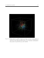
−o p e n g l
:
:
:
:
:
:
:
t h i s s w i t c h a c t i v a t e s t h e 3D−v i s u a l i s a t i o n ou tp ut c a l l s f o r
t h e f o l l o w i n g methods :
SOM − c r i t 2 , SAN, CKM.
This i s o n l y working w i t h o u t p a r a l l e l i z a t i o n and p r o b a b l y on
unix / l i n u x systems
The s o f t w a r e c o m p i l a t i o n has t o be c o n f i g u r e d by
" . / c o n f i g u r e −−e n a b l e −o p e n g l " .
−g l j p e g
: i n c o n j u n c t i o n with −o p e n g l t h i s s w i t c h p r o d u c e s s i n g l e
: jpg−images which can be used t o c r e a t e a n i m a t i o n s .
−g l w i d t h
: width o f o p e n g l g r a p h i c s window ( d e f a u l t =800)
−g l h e i g h t
: h e i g h t o f o p e n g l g r a p h i c s window ( d e f a u l t =800)
−g l p s i z e
: s i z e o f data p o i n t s ( d e f a u l t =0.004D0)
−g l c s i z e
: s i z e o f c e n t r o i d p o i n t s ( d e f a u l t =0.03D0)
−g l x a n g l e <r e a l > : a n g l e t o t i l t view on data cube ( d e f a u l t = −60.D0)
−g l y a n g l e <r e a l > : a n g l e t o t i l t view on data cube ( d e f a u l t = 0 . D0)
−g l z a n g l e <r e a l > : a n g l e t o t i l t view on data cube ( d e f a u l t = 3 5 . D0)
−g l s t e p
: time s t e p p i n g ( d e f a u l t =10)
−g l p a u s e
: pause l e n g t h ( d e f a u l t =1)
−g l b a c k g r o u n d : background c o l o r : 0=b l a c k ( d e f a u l t ) , 1=w h i t e
−g l r o t a n g l e <a n g l e > : r o t a t i o n a n g l e s t e p f o r s p i n n i n g cube
____________________________________________________________________
METHODS:
−met <method>
: method :
: NON| none
: j u s t r e a d ( and w r i t e ) data and e x i t
: INT | i n t e r v a l | BIN :
c l a s s i f y i n t o i n t e r v a l s o f v a r i a b l e −s v a r
:
:
:
:
:
:
:
:
:
GWT| p r o t o t y p e : p r o t o t y p e ’ g r o s s w e t t e r l a g e n ’ , c o r r e l a t i o n based ,
r e s u l t i n g i n 26 t y p e s
GWTWS| gwtws
: based on GWT ( above ) u s i n g 8 t y p e s ,
r e s u l t i n g i n 11 t y p e s
LIT | l i t
: l i t y n s k i t h r e s h o l d s , one c i r c u l a t i o n f i e l d ,
dates , ncl =9|18|27
JCT | j e n k c o l l
: J e n k i n s o n C o l l i s o n scheme
WLK| wlk
: t h r e s h o l d based u s i n g p r e s s u r e , wind ,
t e m p e r a t u r e and humidity
:
:
:
:
:
:
:
PCT|TPC| tmodpca : t−mode p r i n c i p a l component a n a l y s i s o f 10 data
subsets , oblique rotation
PTT|TPT| tmodpcat : t−mode p r i n c i p a l component a n a l y s i s ,
varimax r o t a t i o n
PXE| p c a x t r
: s−mode PCA u s i n g h i g h p o s i t i v e and n e g a t i v e
s c o r e s to c l a s s i f y o b j e c t s
KRZ| k r u i z
: K r u i z i n g a PCA scheme
3 Getting started
14
: LND| lund
: count most f r e q u e n t
: KIR | k i r c h h o f e r : count most f r e q u e n t
: ERP| erpicum
: count most f r e q u e n t
:
distance , adjusting
s i m i l a r p a t t e r n s (− t h r e s )
s i m i l a r p a t t e r n s (− t h r e s )
s i m i l a r patterns , angle
thresholds
: HCL| h c l u s t
:
: h i e r a r c h i c a l c l u s t e r a n a l y s i s ( Murtagh 1 9 8 6 ) ,
s e e parameter −c r i t !
:
:
:
:
:
:
:
:
:
:
: k−means c l u s t e r a n a l y i s ( H a r t i g a n /Wong 1979
algorithm )
: l i k e dkmeans but e v e n t u a l l y s k i p s s m a l l c l u s t e r s
<5% p o p u l a t i o n
: k−means ( s i m p l e a l g o r i t h m ) with most d i f f e r e n t
start patterns
: s i m u l a t e d a n n e a l i n g and d i v e r s i f i e d r a n d o m i s a t i o n
clustering
: s e l f o r g a n i s i n g maps ( Kohonen n e u r a l network )
: P a r t i t i o n i n g Around Medoids
KMN| kmeans
CKM| ckmeans
DKM| dkmeans
SAN | s a n d r a
SOM| som
KMD| kmedoids
: RAN| random
: j u s t p r o d u c e random c l a s s i f i c a t i o n c a t a l o g u e s
: RAC| randomcent : d e t e r m i n e c e n t r o i d s by random and a s s i g n o b j e c t s
:
to i t .
: ASC | a s s i g n
: no r e a l method : j u s t a s s i g n data t o g i v e n
:
c e n t r o i d s p r o v i d e d by −c n t i n
: SUB | s u b s t i t u t e : s u b s t i t u t e c a t a l o g numbers by v a l u e s g i v e n i n a
−c n t i n f i l e
:
: AGG| a g g r e g a t e : b u i l d s e a s o n a l v a l u e s out o f d a i l y o r monthly v a l u e s .
:
: COR| c o r r e l a t e : c a l c u l a t e c o r r e l a t i o n m e t r i c s comparing t h e i n p u t
data v a r i a b l e s .
:
: CNT| c e n t r o i d
: c a l c u l a t e c e n t r o i d s o f g i v e n c a t a l o g (− c l a i n )
:
and data ( s e e −dat ) , s e e a l s o −c n t
:
:
:
:
:
:
:
:
:
:
:
:
:
:
:
:
− c r i t 
ECV| e x v a r
: e v a l u a t i o n o f c l a s s i f i c a t i o n s by E x p l a i n e d
C l u s t e r Variance ( s e e −c l a i n −c r i t )
EVPF| e v p f
: e v a l u a t i o n i n terms o f e x p l a i n e d v a r i a t i o n
and pseudo F v a l u e (− c l a i n )
WSDCIM| wsdcim : e v a l u a t i o n i n terms o f w i t h i n −t y p e SD and
c o n f i d e n c e i n t e r v a l (− c l a i n )
FSIL | f s i l
: e v a l u a t i o n i n terms o f t h e Fast S i l h o u e t t e
Index (− c l a i n )
SIL | s i l
: e v a l u a t i o n i n terms o f t h e S i l h o u e t t e Index
(− c l a i n )
DRAT| d r a t
: e v a l u a t i o n i n terms o f t h e d i s t a n c e r a t i o
w i t h i n and between c l a s s e s (− c l a i n )
CPART| c p a r t
: c a l c u l a t e c o m p a r i s o n i n d i c e s f o r >= 2 g i v e n
p a r t i t i o n s (− c l a i n )
ARI | r a n d i n d e x : c a l c u l a t e o n l y ( a d j u s t e d ) Rand i n d i c e s f o r
two o r more p a r t i t i o n s g i v e n by − c l a i n
: INT | i n t e r v a l :
:
1 = c a l c u l a t e t h r e s h o l d s a s i ’ th p e r c e n t i l e where i=c l ∗1/ n c l
:
2 = b i n s c e n t e r e d around t h e mean v a l u e
:
3 = b i n s i z e i s t h e data−r a n g e / n c l , t h e b i n s a r e not c e n t e r e d .
:
4 = 2 b i n s d i v i d e d by −t h r e s <r e a l > f o r −s v a r .
:
5 = a s 4 but t h r e s h o l d i s i n t e r p r e t e d a p e r c e n t i l e ( 0 t o 1 0 0 ) .
: HCL: ( h i e r a r c h i c a l c l u s t e r i n g ) : number o f c r i t e r i o n :
:
1 = Ward ’ s minimum v a r i a n c e method
:
2 = single linkage
:
3 = complete l i n k a g e
3 Getting started
:
:
:
:
:
:
:
:
:
:
:
:
:
:
:
:
:
:
:
:
:
:
:
:
:
:
:
:
:
:
:
:
:
:
:
:
:
:
:
:
15
4 = average linkage
5 = Mc Quitty ’ s method
6 = median ( Gower ’ s ) method
7 = c e n t r o i d method
GWT:
1 = raw c o e f f i c i e n t s f o r v o r t i c i t y ( d e f a u l t )
2 = normalized v o r t i c i t y c o e f f i c i e n t s
GWTWS:
1 = c l a s s i f i c a t i o n based on a b s o l u t v a l u e s ( d e f a u l t )
2 = c l a s s i f i c a t i o n based on p e r c e n t i l e s
ECV:
1 = monthly n o r m a l i z e d data ( d e f a u l t )
0 = raw data f o r c a l c u l a t i n g e x p l a i n e d c l u s t e r v a r i a n c e .
PCT: r o t a t i o n c r i t e r i a :
1 = d i r e c t o b l i m i n , gamma=0 ( d e f a u l t )
WLK:
0 = u s e raw c y c l o n i c i t y f o r d e c i d i n g a n t i c y c l o n i c o r c y l o n i c
( default )
1 = use anomalies of c y c l o n i c i t y
JCT :
1 = c e n t e r e d c l a s s i f i c a t i o n g r i d with an e x t e n d o f 30 W−E; 2 0 N−S
( default )
2 = c l a s s i f i c a t i o n g r i d e x t e n d e d t o data r e g i o n
SOM:
1 = 1− d i m e n s i o n a l network t o p o l o g y
2 = 2− d i m e n s i o n a l network t o p o l o g y
KMD:
0 = u s e Chebychev d i s t a n c e d=max ( | xa−xb | )
1 = u s e Manhattan d i s t a n c e d=sum ( | xa−xb | )
2 = u s e E u c l i d e a n d i s t a n c e d=s q r t ( sum ( ( xa−xb ) ∗ ∗ 2 ) )
p = u s e Minkovski d i s t a n c e o f o r d e r p : d=(sum ( | xa−xb | ∗ ∗ p ) ) ∗ ∗ ( 1 / p )
PXE/PXK:
0 = o n l y n o r m a l i z e p a t t e r n s f o r PCA ( o r i g i n a l )
1 = n o r m a l i z e p a t t e r n s and n o r m a l i z e g r i d p o i n t v a l u e s a f t e r w a r d s
( default )
2 = n o r m a l i z e p a t t e r n s and c e n t e r g r i d p o i n t v a l u e s a f t e r w a r d s
EVPF, WSDCIM, FSIL , SIL , DRAT:
0 = e v a l u a t e on t h e b a s i s o f t h e o r i g i n a l data v a l u e s
1 = e v a l u a t e on t h e b a s i s o f d a i l y anomaly v a l u e s
2 = e v a l u a t e on t h e b a s i s o f monthly anomlay v a l u e s
BRIER :
1 = q u a n t i l e to absolut values ( d e f a u l t )
2 = q u a n t i l e t o e u c l i d e a n d i s t a n c e s between p a t t e r n s
−t h r e s <r e a l >
: KRC and LND: d i s t a n c e t h r e s h o l d t o s e a r c h f o r key p a t t e r n s
:
d e f a u l t = 0 . 4 f o r k i r c h h o f e r and 0 . 7 f o r lund .
: INT : t h r e s h o l d between b i n s .
: WLK: f r a c t i o n o f g r i d p o i n t s f o r d e c i s i o n on main wind s e c t o r
( d e f a u l t =0.6)
: PXE/PXK: t h r e s h o l d d e f i n i n g key group ( d e f a u l t =2.0)
: BRIER : q u a n t i l e [ 0 , 1 ] ( d e f a u l t =0.9) t o d e f i n e extreme−e v e n t s . An
event i s
:
d e f i n e d when t h e e u c l i d e a n d i s t a n c e t o t h e p e r i o d s / s e a s o n a l / monthly
mean−p a t t e r n
:
i s g r e a t e r than t h e g i v e n q u a n t i l e . I f <t h r e s > i s s i g n e d n e g a t i v e
( e . g . −0.8) ,
:
than e v e n t s a r e d e f i n e d i f s m a l l e r than t h e g i v e n q u a n t i l e .
−s h i f t
: WLK: s h i f t 90 d e g r e e wind s e c t o r s by 45 d e g r e e . D e f a u l t i s no s h i f t .
−n c l 
: number o f c l a s s e s ( must be between 2 and 2 5 6 )
−nrun 
: number o f r u n s ( f o r SAN, SAT, SOM, KMN) f o r s e l e c t i o n o f b e s t r e s u l t .
3 Getting started
:
:
:
:
−s t e p

reduced
16
C l u s t e r a n a l y s i s i s by d e s i g n an u n s t a b l e method f o r complex
datasets .
The more r e p e a t e d r u n s a r e used t o s e l e c t t h e b e s t r e s u l t t h e more
robust
i s t h e r e s u l t . SOM and SAN a r e d e s i g n e d t o be much more r o b u s t than
KMN.
d e f a u l t = −nrun 1000 t o p r o d u c e r e l i a b l e r e s u l t s !
: SOM: number o f e p o c h s a f t e r which n e i g h b o u r h o o d r a d i u s i s t o be
:
:
:
:
:
:
:
:
:
:
For t r a i n i n g t h e neurons , a l s o n e i g h b o u r e d n e u r o n s o f t h e wi nne r
neuron
i n t h e network−map a r e a f f e c t e d and adapted t o t h e t r a i n i n g p a t t e r n
( to a
l o w e r d e g r e e though ) . The n e i g h b o u r h o o d r a d i u s c o v e r s a l l n e u r o n s
( classes
a t t h e b e g i n n i n g and i s r e d u c e d d u r i n g t h e p r o c e s s u n t i l o n l y t h e
wi nne r neuron
i s a f f e c t e d . This s l o w d e c r e a s e h e l p s t o overcome l o c a l minima i n
the o p t i m i s a t i o n
function .
d e f a u l t = −s t e p 10 ( meaning a f t e r 10 e p o c h s n e i g h b o u r h o o d r a d i u s i s
reduced
by one ) .
WLK: number o f w i n d s e c t o r s
EVPF, WSDCIM, FSIL , SIL , DRAT, CPART: m i s s i n g v a l u e i n d i c a t o r f o r
c a t a l o g u e data
− i t e r 
: SOM, PXE, PXK: maximum number o f e p o c h s / i t e r a t i o n s t o run
:
d e f a u l t = − i t e r 2 0 0 0 , i . e . i t s h o u l d c o n v e r g e by i t s e l f
: − i t e r 0 f o r p c a x t r means t h a t o n l y t h e f i r s t a s s i g n m e n t t o t h e
pc−c e n t r o i d s i s done .
:
f o r PXK − i t e r i s 2000 ( means 2000 k−means i t e r a t i o n s )
−temp <r e a l >
: s i m u l a t e d a n n e a l i n g s t a r t t e m p e r a t u r e ( f o r CND)
:
default = 1
−c o o l <r e a l >
: c o o l i n g r a t e ( f o r som & s a n d r a )
:
d e f a u l t = −c o o l 0 . 9 9 D0 ; s e t t o 0 . 9 9 9 D0 o r c l o s e r t o 1 . D0 t o
enhance ( and s l o w down ) .
−s v a r 
: tuning parameter
: INT : number o f v a r i a b l e / column t o u s e f o r c a l c u l a t i n i n t e r v a l
thresholds .
−a l p h a <r e a l >
: tuning parameter
: WLK: c e n t r a l w e i g h t f o r w e i g h t i n g mask ( d e f a u l t =3.D0)
: EVPF, WSDCIM, FSIL , SIL , DRAT: s c a l e f a c t o r f o r e v a l u a t i o n data
: BRIER :
:
i f < 0 => ( d e f a u l t ) u s e a l l v a l u e s (− c r i t 1 ) o r p a t t e r n s (− c r i t 2 )
:
i f >=0 => a v a l u e o r p a t t e r n i s p r o c e s s e d o n l y i f i t s e l f o r
mean ( p a t t e r n ) > a l p h a .
: GWTWS: v a l u e / p e r c e n t i l e f o r low winds ( main t h r e s h o l d f o r t y p e s
9 ,10 ,11)
−b e t a <r e a l >
: tuning parameter
: WLK: mi dd le zone w e i g h t f o r w e i g h t i n g mask ( d e f a u l t =2.D0)
: EVPF, WSDCIM, FSIL , SIL , DRAT: o f f s e t v a l u e f o r e v a l u a t i o n data
: GWTWS: v a l u e / p e r c e n t i l e f o r f l a t winds ( t y p e 1 1 )
−gamma <r e a l >
: tuning parameter
: WLK: margin zone w e i g h t f o r w e i g h t i n g mask ( d e f a u l t =1.D0)
3 Getting started
:
:
−d e l t a <r e a l >
17
WSDCIM: c o n f i d e n c e l e v e l f o r e s t i m a t i n g t h e c o n f i d e n c e i n t e r v a l o f
t h e mean
GWTWS: v a l u e / p e r c e n t i l e f o r low p r e s s u r e ( t y p e 9 )
: tuning parameter
: WLK: width f a c t o r f o r w e i g t h i n g z o n e s ( nx∗ d e l t a | ny∗ d e l t a )
( d e f a u l t =0.2)
: PXE/PXK: s c o r e l i m i t f o r o t h e r PCs t o d e f i n e u n i q u e l y l e a d i n g PC
( default 1.0)
: GWTWS: v a l u e / p e r c e n t i l e f o r h i g h p r e s s u r e ( t y p e 1 0 )
−lambda <r e a l > : t u n i n g p a r a m e t e r
: SAT :
w e i g h t i n g f a c t o r f o r time c o n s t r a i n e d c l u s t e r i n g
( d e f a u l t =1.D0)
− d i s t 
: d i s t a n c e m e t r i c ( not f o r a l l methods y e t ) :
:
i f i n t > 0 : Minkowski d i s t a n c e o f o r d e r i n t (0= Chebychev ) ,
:
i f i n t =−1: 1− c o r r e l a t i o n c o e f f i c i e n t .
−nx 
: KIR : number o f l o n g i t u d e s , needed f o r row and column c o r r e l a t i o n s
: DRAT: d i s t a n c e measure t o u s e (1= e u c l i d e a n d i s t a n c e , 2=p e a r s o n
correlation )
−ny 
: KIR : number o f l a t i t u d e s
−wgttyp e u c l i d | normal : a d j u s t w e i g h t s f o r s i m u l a t i n g E u c l i d e a n d i s t a n c e s o f o r i g i n a l
:
data o r not .
____________________________________________________________________
OTHER:
−v 
yet ) ,
: v e r b o s e : d e f a u l t = ’−v 0 ’ , i . e . q u i e t ( not working f o r a l l r o u t i n e s
: 0 = show n o t h i n g , 1 = show e s s e n t i a l i n f o r m a t i o n , 2 = i n f o r m a t i o n
about r o u t i n e s
: 3 = show d e t a i l e d i n f o r m a t i o n s about r o u t i n e s work ( s l o w s down
computation s i g n i f i c a n t l y ) .
−h e l p
: g e n e r a t e t h i s o ut pu t and e x i t
____________________________________________________________________
4 Data input
18
4 Data input
The first step of a cost733class run is to read input data. Depending on the use case
these data can have very different formats. Principally there are two kinds: Foreign data
were not produced by cost733class, whereas self-generated indeed are.
4.1 Foreign formats
cost733class can read any data in order to classify it. It is originally made for weather
and circulation type classification but most of the methods are able to classify anything,
regardless of the meaning of the data (only in some cases information about dates and
spatial coordinates are necessary). The concept of classification is to define groups,
classes or types (all these terms are used equivalently) encompassing objects, entities,
cases or objects (again these terms mean more or less the same) belonging together. The
rule how the grouping should be established differs from method to method, however
in most of the cases the similarity between objects is utilized, while the definition of
similarity differs again. In order to distinguish between various objects and to describe
similarity or dissimilarity, each object is defined by a set of attributes or variables (this is
what an entity is made of). A useful model for the data representation is the concept of
a rectangular matrix, where each row represents one object and each column represents
one attribute of the objects. In case of ASCII-formatted input data this is exactly the
way how the input data format is defined.
4.1.1 ASCII data file format
ASCII text files have to be formatted in such a way that they contain the values of one
object (time slice) in one line and the values for one variable (commonly a grid point)
in a column. For more than one variable (grid point) the following columns have to be
separated by one or more blank letters (" "). Note that tabulator-characters (sometimes
used by spread sheet programs as default) are not sufficient to separate columns! The file
should contain a rectangular input matrix of numbers, i.e. constant number of columns
at each row and a constant number of rows for each column. No missing values are
allowed. The software evaluates an ASCII file on its own to find out the number of lines
(days, objects, entities) and the number of variables (attributes, parameters, grid points).
For this the numbers in one line have to be separated by one or more blanks (depending
on the compiler commas or slashes may also be used as separators between different
4 Data input
19
numbers, but the comma never as decimal marker!!! The decimal marker must always
be a point!). Thus you don’t have to tell how many lines and columns are in the file,
but the number of columns has to be constant throughout the file (the number of blanks
between two attributes may vary though). This format is fully compatible to the CSV
(comma separated values) format which can be written e.g. by spread sheet calculation
programs. Note that no empty line is allowed. This can lead to read errors especially
if there is an empty line at the bottom of the file which is hard to see. If necessary,
information about time and grid coordinates describing the data set additionally have
to be provided within the data set specification at the command line. In this case the
ordering of rows and columns in the file must fit the following scheme: The first column
is for the southernmost latitude and the westernmost longitude, the second column for
the second longitude from west on the southernmost latitude, etc. The last column is
for the easternmost and northernmost grid point. The rows represent the timesteps. All
specifications have to fit to the number of rows and columns in the ASCII file.
4.1.2 COARDS NetCDF data format
Cost733class includes the NetCDF library and is able to read NetCDF files directly and
use the information stored in this self describing data format. It has been developed using
6-hourly NCEP/NCAR reanalysis data (Kalnay et al., 1996), which are described and
available at: http://www.cdc.noaa.gov/data/gridded/data.ncep.reanalysis.html
but also other data sets following the COARDS conventions
(http://ferret.wrc.noaa.gov/noaa_coop/coop_cdf_profile.html) should be readable if they use the time unit of hours since 1-1-1 00:00:0.0 or any other year. In
case of multi-file data sets the files have to be stored into one common directory and
a running number within the file names has to be indicated by ? symbols, which are
replaced by a running number given by the fdt: and ldt: flag (see below). Information
about time and grid coordinates of the data set are retrieved from the NetCDF data
file automatically. In case of errors resulting from buggy attributes of the time axis in
NetCDF files try -readncdate. Then the dates of observations are retrieved from the
NetCDF time variable rather than calculating it from "actual range" attribute of the
time variable.
4.1.3 GRIB data format
Cost733class includes the GRIB_API package and is able to read grib (version 1 &
2) files directly and use the information stored in this self describing data format. It
has been developed using 6-hourly ECMWF data, which are described and available at:
http://data-portal.ecmwf.int/data/d/interim_daily/
In case of multi-file data sets the filepaths have to contain running numbers indicated
by ? symbols, or a combination of the following strings: YYYY / YY, MM, DD / DDD ;
they are replaced by running numbers given by the fdt: and ldt: flags (see below).
4 Data input
20
Information about time and grid coordinates of the data set are retrieved from the grid
data file automatically.
4.1.4 Other data formats
At the moment there is no direct support for other data formats. Also it may be
necessary to convert NetCDF-files first if e.g. the time axis is not compatible. A good
choice in many aspects might be the software package CDO (climate data operators):
https://code.zmaw.de/projects/cdo which is released under GNU General Public
License v2 (GPL). Attention has to be paid to the type of calendar used. It can be
adjusted by
cdo s e t r e f t i m e ,1 −01 −01 ,00:00 , h o u r s −s e t c a l e n d a r , s t a n d a r d i n p u t . nc o ut pu t . nc
where hours has to be replaced e.g. by days or another appropriate time step if the
time step given in the input file differs.
4.2 Self-generated formats
4.2.1 Binary data format
Binary data files are those written with form="unformatted" by FORTRAN programs.
For input their structure has to be known and provided by the specifications @lon:,
@lat:, @fdt:, @ldt: and eventually @ddt: and @mdt. Reading of unformatted data is
consideraly faster than reading formatted files. Therefore it might be a good idea to use
the -writedat option to create a binary file from one or more other files if many runs
of cost733class are planned. If the extension of the file name is *.bin, unformatted
files are assumed by the program.
4.2.2 Catalog files
For some procedures (like comparison, centroid calculation, assignment of data to existing catalogs, etc.) it is necessary to read catalog files from disk. This is done using the
option -clain <spec>, where the specification <spec> is similar to the specification of
the data input option. The following specifications are recognized:
• @pth:<file name>
• @fdt:<first date>
• @ldt:<last date>
• @ddt:<time step, e.g. "@ddt:1d" for one day>
4 Data input
21
• @dtc:<number of date columns>
• @mdt:<list of months> e.g. @mdt:01,02,12
See specifying data input for more details on these specifications. As with the data
input, more than one classification catalog file may be used by providing more than one
-clain option. Note that all catalog files have to be specified with all necessary flags.
Especially a wrong number of date columns could lead to errors in further steps.
4.2.3 Files containing class centroids
For the assignment to existing classifications it can be necessary to read files that contain
class centroids. This is done with the -cntin <filename> option. Allthough there is
support for NetCDF output of class centroids in cost733class at the time only ASCII
files are supposed to be read successfully. A suitable file might be generated with the
-cnt <filename> option in a previous run. The extension of <filename> must be .dat.
For further information see section 7.1.
Considering that such files can also be easily written with any text editor this feature
of cost733class makes it possible to predefine class centroids or composites and assign
data to them.
4.3 Specifying data input and preprocessing
The data input and preprocessing steps are carried out in the following order:
1. reading input data files (pth:)
2. grid point selection (slo: and sla:)
3. data scaling (scl:)
4. adding offset (off:)
5. centering/normalization of object (nrm:)
6. calculation of anomalies (ano:)
7. filtering (fil:)
8. area weighting (arw:)
9. sequence construction (seq:)
10. date selection (options -dlist, -per, -mon, -hrs)
11. PCA of each parameter/data set separately (pca:, pcw:)
4 Data input
22
12. parameter weighting (wgt:)
13. overall PCA (options -pca, -pcw)
For reading data sets, the software first has to know how many variables (columns)
and time steps (rows) are given in the files. In case of ASCII files the software will
find out these numbers by its own, if no description is given. However in this case no
information about time and space is available and some functions will not work. In
case of NetCDF files this information is always given in the self describing file format.
Thus the description of space and time by specification flags on the command line can
be omitted but will be available. Some methods like lit need to know about the date
(provided e.g. by -per, -mon, etc.) of each object (e.g. day), or the coordinates (provided
by @lon: and @lat:) while other methods do not depend on it. If necessary the given
dates of a data set have to be described for each data set (or the first in case of same
lengths) separately (see @fdt:, @ldt: and @ddt: or @dtc:).
After the data set(s) is(are) loaded some selections and preprocessing can be done,
again by giving specification flags (key words for only one single data set without a
leading -) and options (keywords which are applied to all data sets together with a
leading -).
4.3.1 Specification flags
In order to read data from files which should be classified, these data have to be specified
by the -dat <specification> option.
It is important to distinguish between specification flags to describe the given data
set as contained in the input files on the one hand and flags and options to select or
preprocess these data.
The <specification> is a text string (or sequence of key words) providing all information needed to read and process one data set (note that more data sets can be read,
thus more than one specifications are needed). Each kind of information within such a
string (or key word sequence) is provided by a <flag> follwed by a : and a <value>. The
different information substrings have to follow the -dat option, i.e. they are recognized
to belong together to one data set as long as no other option beginning with - appears.
They may be concatenated by the @ separator symbol directly together (without any
blank (" ") inbetween) or they may be separated by one or more blanks. The order
of their appeareance is not important, however if one flag is provided more than once,
the last one will be used. Please note that flags differ from options by the missing (leading minus). The end of a specification of a data set is recognized by the occurence
of an option (i.e. by a leading -).
The following flags are recognized:
4 Data input
23
4.3.2 Flags for data set description
• var:<character>
This is the Name of the variable. If the data are NetCDF files this must be exactly
the variable name as in the NetCDF file, else it could not be found resulting in an
error. If this flag is omitted the program tries to find the name on its own. This
name is also used to construct the file names for NCEP/NCAR Reanalysis data
file (see the pth: flag). In case the format is ASCII the name is not important and
this flag can be omitted, except for special methods based on special parameters
(e.g. the wlk-method needs uwnd, vwnd, etc.). The complete var flag might look
e.g. like: var:slp
• pth:<character>
– In case of ASCII format this is the path of the input file (its location directory
including the file name). Please note that, depending on the system, some
shortcuts for directories may not be recognized, like the symbol for the home
directory. E.g.: pth:/home/user/dat/slp.txt.
– In case of a fmt:netcdf data set consisting of multiple subsequent files the
path can include ? symbols to indicate that these letters should be replaced by
a running number between the number given by fdt: and the number given by
ldt: . E.g. pth:/geo20raid/dat/ncep/slp.????.nc fdt:1948 ldt:2010
(for a NetCDF multifile data set).
– In case of fmt:grib the file name/path can include ? symbols, or a
combination of the following strings: YYYY / YY, MM, DD / DDD ; to indicate that these letters should be replaced by a running number between the number given by fdt: and the number given by ldt:, which
has to have the same order and format as given in the path. E.g.
pth:/data/YYYY/MM/slp.DD.grib fdt:2011:12:31 ldt:2012:01:01 or
pth:/data/slp.YYYY-MM-DD.grib fdt:2011:12:31 ldt:2012:01:01 or
pth:/data/slp.MMDDYYYY.grib fdt:12:31:2011 ldt:01:01:2012 or
pth:/data/slp.YYYY.grib fdt:2011:12:31 ldt:2012:01:01 or
pth:/data/slp.YYYYDDD.grib fdt:2011:001 ldt:2012:365
(for grib multifile data sets).
• fmt:<character>
This can be either ASCII, binary or NetCDF. ftm:ascii means the data are
organized in text files: Each line holds one observation (usually the values of a
day). Each column holds one parameter specifying the observations. Usually the
columns represent grid points. These files have to hold a rectangular matrix of
values, i.e. all lines have to have the same number of columns. Columns have to
be separated by one or more blanks (" ") or by commas. Missing values are not
4 Data input
24
allowed. The decimal marker must be a point!
fmt:netcdf means the data should be extracted from NetCDF files. If the file
name extension of the provided file name is .nc NetCDF format is assumed.
The information about data dimensions are extracted form the NetCDF files.
fmt:binary denotes unformatted data. The dimensions of the data set have to
provided by the specifications @lon:, @lat:, @fdt:, @ldt: and eventually @ddt:
and @mdt. This format is assumed if the file name extension is bin. The default,
which is assumed if no fmt: flag is given, is ASCII.
• dtc:<integer>
If the file format is fmt:ascii and there are leading columns specifying the date
of each observation, this flags has to be used to specify how many date columns
exist: "1" means that there is only one date column (the first column) holding the
year, "2" means the two first columns hold the year and the month, "3" means
the first three columns hold the year, the month and the day and "4" means the
first four coluns holds the year, month, day and hour of the observation.
• fdt:YYYY:MM:DD:HH
first date of data in data file (date for first line or row). Hours, days and months
may be omitted. For data with fmt:netcdf in multiple files, it can be an integer
number indicating the first year or running number which will be inserted to replace
the ? placeholder symbols in the filename.
• ldt:YYYY:MM:DD:HH
last date of data in data file (date for last line or row). Hours, days and months
may be omitted. If so and ldt indicates a number of rows smaller than actually
given in the file, only this smaller number of lines is used (omitting the rest of
the file). For data with fmt:netcdf in multiple files, it can be an integer number
indicating the last year or running number which will be inserted to replace the ?
placeholder symbols in the filename.
• ddt:<int><y|m|d|h>
time step of dates in data file in years, months, days or hours, e.g.: 1d for daily data.
If ddt is omitted but both, fdt and ldt have same resolution it is automatically
set to one for that temporal resolution, e.g.: fdt:1850:01 and ldt:2008:02 and
omitting ddt will lead to ddt:1m, i.e. monthly resolution.
• mdt:<list>
list of months covered in data file, e.g. mdt:01:02:12 if only winter data are given
in the file. The list separator symbol may also be the comma "," instead of the
":".
• lon:<number>:<number>:<number>
This specifies the longitude dimensions of the input data as given in the file. The
4 Data input
25
first <number> is the minimum longitude where longitudes west of 0 degree are
given by negative numbers. The second <number> is the maximum longitude. The
third <number> is the grid spacing in longitudes. e.g.: lon:-30:50:2.5 This flag
denotes just the description of the input data. For NetCDF data (which are self
describing) it is superflous!
• lat:<number>:<number>:<number>
This specifies the latitude dimensions of the input data. The first <number> is
the minimum latitude where latitudes south of the equator are given by negative
numbers. The second <number> is the maximum latitude. The third <number>
is the grid spacing in latitudes. e.g.: lat:30:70:2.5 Note that at the moment
south-to-north order must be given in the dat file, i.e. the left columns hold the
southern-most latitudes.
4.3.3 Flags for spatial data Selection
• slo:<number>:<number>:<number>
If given, this flag selects a subset of grid points from the grid in the input data.
The first <number> is the minimum longitude where longitudes west of 0 degree
are given by negative numbers. The second <number> is the maximum longitude.
The third <number> is the grid spacing in longitudes. The user must take care
that the selected grid fits into the given grid!
• sla:<number>:<number>:<number>
If given, this flag selects a subset of grid points from the grid in the input data.
The first <number> is the minimum latitude where latitudes south of the equator
are given by negative numbers. The second <number> is the maximum latitude.
The third <number> is the grid spacing in latitudes. The user must take care that
the selected grid fits into the given grid!
• sle:<integer>
This flag specifies the atmospheric level to be read if the fmt:ncepr flag is given.
This is relevant for NetCDF data which may contain data of more than one level.
If omitted the first level in the file is selected.
4.3.4 Flags for data Preprocessing
• seq:<integer>
This specifies whether this input data matrix should be extended in order to build
sequences of observations for the classification. The <integer> specifies the length
of the sequence. If this flag isn’t provided then the sequence length is "1", i.e. no
extension will be made. If it is "2" then one copy of the data matrix (shifted
by one row/time step into the past) will be concatenated to the right side of the
4 Data input
26
original data matrix, resulting in a doubling of the variables (columns). This
copy is shifted by 1 observation (line) downwards, thus each line holds the values
of the original variable and the values of the preceeding observation (e.g. day).
In this way each observation is characterised additionally by the information of
the preceeding observation and the history of the variables are included for the
classification. <integer> can be as high as desired, e.g. 12 for a sequence of 12
observations. In order to keep the original number of observations for the first lines
(which do not have preceeding observations) the values of the same observation
are copied to fill up the gaps.
• wgt:<number>
If more than one data set is given each data set can be weighted relative to others,
i.e. its values count more (or less) for determination of the similarity between the
observations. If this flag is omitted the weight is 1.0 for all data and all data sets
(each one defined by a -dat specification) are treated to have the same weight
compared to each other by normalizing them separately as a whole (over space
and time) and multiplying them with a factor 1/nvar, where nvar is the number
of variables or attributes of each data set. After that each datasset is multiplied
by the user weight <number>.
• scl:<float>
Scaling factor to apply to the input data of this parameter.
• off:<float>
Offset value which will be added to input data after scaling.
• nrm:<integer>
row-wise normalisation: 1 = row-wise centralisation of objects/patterns, 2 = rowwise normalisation of objects/patterns (sample standard deviation), 3 = row-wise
normalisation of objects/patterns (population standard deviation)
• ano:<integer>, where integer can be
-1 : column wise centralisation of variables (grid points) after selection of time
steps
-2 : column wise normalisation of variables using sample standard deviation
(sum of squared deviations divided by n) after selection of time steps
-3 : column-wise normalisation of variables using population standard deviation
(sum of squared deviations divided by n-1) after selection of time steps
1 : column wise centralisation of variables (grid points) before selection of time
steps
2 : column wise normalisation of variables using sample standard deviation
(sum of squared deviations divided by n) before selection of time steps
4 Data input
27
3 : column-wise normalisation of variables using population standard deviation
(sum of squared deviations divided by n-1) before selection of time steps
11 column-wise centralisation of variables using the daily long-term mean for
removing the annual cycle
12 column-wise normalisation of variables using the daily long-term mean and
sample standard deviation for removing the annual cycle,
13 column-wise normalisation of variables using the daily long-term mean and
population standard deviation for removing the annual cycle,
21 column-wise centralisation of variables using the monthly long-term mean for
removing the annual cycle,
22 column-wise normalisation of variables using the monthly long-term mean
and sample standard deviation for removing the annual cycle,
23 column-wise normalisation of variables using the monthly long-term mean
and population standard deviation for removing the annual cycle,
31 column-wise centralisation of variables using the daily long-term mean of 31day wide moving windows for removing the annual cycle
32 column-wise normalisation of variables using the daily long-term mean and
sample standard deviation of 31-day wide moving windows for removing the
annual cycle
33 column-wise normalisation of variables using the daily long-term mean and
population standard deviation of 31-day wide moving windows for removing
the annual cycle
• fil:<integer>
gaussian time filter of period <int>; int<0 = high-pass, int>0 = low-pass
• arw:<integer>
Area weighting of input data grids: 0 = no (defaut), 1 = cos(latitude), 2 =
sqrt(cos(latitude)), 3 = calculated weights by area of grid box which is the same
as cos(latitude) of option 1.
• pca:<integer|float>
parameter-wise pca: If provided, this flag triggers a principal component analysis
for compression of the input data. The PCA retains as many principal components
as needed to explain at least a fraction of <real> of the total variance of the data
or as determined by <integer>. This can speed up the classification for large data
sets considerably. Useful values are 0.99 or 0.95.
• pcw:<integer|float>
parameter-wise pca with weighting of scores by explained variance: This preprocessing step works like pca but, weights the PCs according to their explained
4 Data input
28
variance. This simulates the original data set in contrast to the unweighted PCs.
In order to simulate the Euclidean distances calculated from the original input
data (for methods depending on this similarity metric), the scores of each PC are
weighted by sqrt(exvar(PC)) if -wgttyp euclid is set. Therefore if -pcw 1.D0 is
given (which actually doesn’t lead to compression since as may PCs as original
variables are used) exactly the same euclidean distances (relative to each other)
are calculated.
4.3.5 Flags for data Postprocessing
• cnt:<file>.<ext>
write parameter composit (centroid) to file of format depending on extension: .txt
= ascii-xyz data, .nc = netcdf,
4.3.6 Options for selecting dates
If there is at least one input data set with given flags for date description, this information
about the time dimension can be used to select dates or time steps for the procedure.
Such a selection applies to all data sets if more than one is used.
Note that the following switches are options beginning by a - because they apply to
the whole of the data set:
• -per YYYY:MM:DD:HH,YYYY:MM:DD:HH,nX
This option selects a certain time period, starting at a certain year (1st YYYY),
month (1st MM), day (1st DD) and hour (1st HH), ending at another year (2nd
YYYY), month (2nd MM), day (2nd DD) and hour (2nd HH), and stepping by n
time units (nX). The stepping information can be omitted. Time unit X can be:
– y for years
– m for months
– d for days
– h for hours. Stepping for hours must be 12, 6, 3, 2 or 1
The default stepping is 1 while the time unit for the stepping (if omitted) is
assumed to be the last date description value (years if only is given YYYY, months
if also MM is provided, days for DD or hours for HH).
• -mon 1,2,3
In combination with the -per argument the number of months used by the software
can be restricted by the -mon option followed by a list of month numbers.
• -dlist <file>
Alternatively it is possible to select time steps (continuously or discontinously) and
4 Data input
29
for both NetCDF and ASCII data by the -dlist <file> option. The given file
should hold as many lines as time steps should be selected and four columns for
the year, month, day and hour of the time step. These numbers should be integer
and separated by at least one blank. Even if no hours are needed they must be
given as a dummy.
Note that it is possible to work with no (or fake) dates, allowing for input of ASCIIdata sets which have been selected by another software before.
4.3.7 Using more than one data set
More than one data set can be used by just giving more than one -dat <specification>
option (explained above) within the command line. The data of a second (or further)
data set are then pasted behind the data of the first (or previous) data set as additional
variables (e.g. gridpoints or data matrix columns) thus defining each object (e.g. day or
data matrix rows) additionally. Note that these data sets must have the same number
of objects (lines or records) in order to fit together.
If one of the data sets is given in different physical units than the others (e.g. hPa
and Kelvin), there must be taken care of the effect of this discrepancy for the distance
metric used for classification.
1. For all metrics the data set with higher total variance (larger numbers) will have
larger influence.
2. For correlation based metrics, if there is a considerable difference of the mean
between two data sets, this jump can result in strange effects. E.g. for t-mode
PCA (PPT) there might be just one single class explaining this jump while all
other classes are empty.
Therefore in case of using more than one data set (i.e. multifield classification) each
data set (separately from the others) should be normalized as a whole (one single mean
and standard deviation for all columns and rows of this single data set together). This
can be achieved by using the flag
• @wgt:<float>
at least for one data set. Where <float> can be 1.D0 (the D is for double precision) in
order to apply a weight of 1.0.
If a weighting factor is given using the flag @wgt:<float>, the normalized data sets
are multiplied with this factor respectively. The default value is 1.D0, however it will
be applied only if at least for one data set the flag @wgt:<float> is given! If this is the
case, always all data sets will be normalized and weigthed (eventually with 1.D0 if no
individual weight is given).
4 Data input
30
In case of methods using the Euclidean distance the square root of the weight is used
in order to account for the square in the distance calculations. This allows for a correct
weight of the data set in the distance measure. Also different numbers of variables (grid
points) are accounted for by dividing the data by the number of variables. Therefore
the weight is applied to each data set as a whole in respect to the others. If e.g. a
weight of 1.0 is given to data set A (@wgt:1.0) and a weight of 0.5 is given to data set
B (@wgt:0.5) then data set A has a doubled influence on the assignement of objects to
a type compared to data set B, regardless how many variables (grid points) data set A
or B has and regardless what the units of the data has been.
It is advisable always to specify the @wgt:<float> flag for all data sets if multiple
data sets are used. E.g.
c o s t 7 3 3 c l a s s −dat pth : s l p . txt@wgt : 1 . D0 −pth : shum . txt@wgt : 1 . D0 −met XYZ
4.3.8 Options for overall PCA preprocessing of all data sets
together
Apart from the possibility to apply Principal Component Analyis to each parameter
data set separately, the option -pca <float|integer> allows a final PCA of the whole
data set. As with the separate procedure the number of PC’s to retain can be given as
an integer number or, in case of a floating number, the fraction of explained variance
to retain can be specified. Also automatic weighting of each PC with it’s fraction of
explained variance can be obtained by using the -pcw <float|int> flag instead of -pca.
4.4 Examples
4.4.1 Simple ASCII data matrix
c o s t 7 3 3 c l a s s −dat pth : era40_MSLP . dat@fmt : a s c i i @ l o n : − 3 7 : 5 6 : 3 @lat : 3 0 : 7 6 : 2 −met kmeans
−n c l 9
This will classify data from an ASCII file (era40_MSLP.dat) which holds as many
columns as given by the grid of -37 to 56 degree longitude (3 degree spacing) and 30 to
76 degree latitude (2 degree spacing). Thus the file has (56-(-37))/31 by (76-30)/2+1
columns (=32x24=768). The ordering of the columns follows the principle: longitudes
vary fastest from west to east, latitudes vary slowest from south to north. Thus the
first column is for the southernmost latitude and the westernmost longitude, the second
column for the second longitude from west on the southernmost latitude, etc. The last
column is for the easternmost and northernmost grid point as illustrated in table 4.4.1
Note that the command line could have been written as
c o s t 7 3 3 c l a s s −dat pth : era40_MSLP . dat l o n : − 3 7 : 5 6 : 3 l a t : 3 0 : 7 6 : 2 −met kmeans −n c l 9
4 Data input
t=1
t=2
...
t=nt
31
colum #1
lon=-37,lat=30
mslp(-37,30,1)
mslp(-37,30,2)
...
mslp(-37,30,nt)
column #2
lon=-34,lat=30
mslp(-34,30,1)
mslp(-34,30,2)
...
mslp(-34,30,nt)
...
...
...
...
...
column #32
lon=56,lat=30
mslp(56,30,1)
mslp(56,30,2)
...
mslp(56,30,nt)
column #33
lon=-37,lat=32
mslp(-37,32,1)
mslp(-37,32,2)
...
mslp(-37,32,nt)
...
...
...
...
...
column #768
lon=56,lat=76
mslp(56,76,1)
mslp(56,76,2)
...
mslp(56,76,nt)
Table 4.1: Example data matrix of mean sea level pressure values formatted to hold grid
points in columns varying by lon = −37, 56 by 3◦ and by lat = 30, 76 by 2◦
and time steps t = 1, nt in rows.
2000
2000
2000
2000
2000
2000
2000
2000
2000
2000
2000
2000
2000
2000
...
2008
01
01
01
01
01
01
01
01
01
01
01
01
01
01
...
12
01
02
03
04
05
06
07
08
09
10
11
12
13
14
...
31
-12.1
-10.3
-6
-7.3
-7.7
-6.6
-8
-9.1
-10.3
-11.1
-12
-8.7
-11.2
-9.6
...
-8
Table 4.2: Example ASCII file contents including three date columns for year, month
and day.
to achieve exactly the same result. All flags are recognized to belong to the -dat option
until another option beginning with - appears. Note that in this example no information
about the time was made, i.e. the date of each line is unknown to the program. In this
case this is unproblematic because k-means doesn’t care about the meaning of objects,
it just classifies it according to their attriubtes (the pressure values at the grid points in
this case).
4.4.2 ASCII data file with date columns
c o s t 7 3 3 c l a s s −dat pth : s t a t i o n / z u g s p i t z e _ 2 0 0 0 −2008_Tmean . dat d t c : 3 ano : 3 3 −met BIN −n c l
10
In this example the software is told, that there are three leading comluns in the file
holding the date of each line (year, month, day because there are 3 columns and this is
the hierarchy per definition, there is no way to change this order). The total number
of columns (four) and the number of rows is detected by the software itself by counting
the blank-gaps in the lines. The beginning of this file looks like shown in table 4.4.2
Also there is an option ano:33 in order to use the anomalies (deviation) referring to
the long-term daily mean. Afterwards the method BIN is called which by default just
4 Data input
32
calculates equally spaced percentile thresholds to define 10 (-ncl 10) classes, to which
the data is assigned. Note that this method uses only the first column (after any date
columns of course).
4.4.3 NetCDF data selection
c o s t 7 3 3 c l a s s −dat v a r : hgt@pth : / data /20thC_ReanV2/ hgt . ? ? ? ? . nc f d t : 1 8 7 1 l d t : 2 0 0 8 \
s l o : −50:50:2.0 s l a : 2 0 : 5 0 : 2 . 0 s l e :0950 \
−w r i t e d a t hgt_0950_slo −50−50_sla −20−50_1871 −2008. b i n
This command selects a subgrid from 50◦ west to 50◦ east by 2◦ and from 20◦ north to
50◦ north (by 2◦ ) out of the global reanalysis (20thC_ReanV2) grid. After input in this
case the data are written to a binary file, which can be used for further classification by
subsequent runs. But of course it would have been possible to provide a -met option to
start a classification in this run. Note that this call needs 1.2 GB of memory.
4.4.4 Date selection for classification and centroids
s r c / c o s t 7 3 3 c l a s s −dat pth : g r i d / s l p . dat \
lon : −10:30:2.5
l a t : 3 5 : 6 0 : 2 . 5 f d t : 2 0 0 0 : 1 : 1 l d t : 2 0 0 8 : 1 2 : 3 1 ddt : 1 d \
−met CKM −n c l 8 −p e r 2 0 0 0 : 1 : 1 , 2 0 0 8 : 1 2 : 3 1 , 1 d −mon 6 , 7 , 8 −v 3
s r c / c o s t 7 3 3 c l a s s −dat pth : g r i d / s l p . dat \
lon : −10:30:2.5
l a t : 3 5 : 6 0 : 2 . 5 f d t : 2 0 0 0 : 1 : 1 l d t : 2 0 0 8 : 1 2 : 3 1 ddt : 1 d c n t :DOM00. nc \
− c l a i n pth :CKM08. c l a d t c : 3 f d t : 2 0 0 0 : 6 : 1 l d t : 2 0 0 8 : 8 : 3 1 mdt : 6 : 7 : 8 \
−p e r 2 0 0 0 : 1 : 1 , 2 0 0 8 : 1 2 : 3 1 , 1 d −mon 6 , 7 , 8 \
−met CNT −v 3
Here classification is done only for summer months (-per 2000:1:1,2008:12:31,1d
-mon 6,7,8) and written to CKM08.cla in the first run. In the second call CKM08.cla
is used to build centroids, again only for the summer months. Note that mdt:6:7:8 has
to be provided for the -clain option in order to read the catalog correctly.
5 Data output
33
5 Data output
5.1 The classification catalog
This is a file containing the list of resulting class numbers. Each line represents one classified entity. If date information on the input data was provided the switch -dcol <int>
can be used to write the datum to the classification outputfile as additional columns left
to the class number. The argument <int> decides on the number of date columns:
-dcol 1 means only one column for the year or running number in case of fake dates
(1i4), -dcol 2 means year and month (1i4,1i3), -dcol 3 means year, month and day
(1i4,2i3) and -dcol 4 means year, month, day and hour (1i4,3i3). If the -dcol option
is missing the routine tries to guess the best number of date columns. This number
might be important if the catalog file is used in subsequent runs of cost733class e.g. for
evaluation etc.
5.2 Centroids or type composits
If the -cnt <filename> option is given, a file is created which contains the data of the
centroids or class means. In each column of the file the data of each class is written. Each
line/row of the file corresponds to the variables in the order (of the columns) provided
in the input data.
If the cnt:<file.nc> flag has been given within the individual specification of a data
set, the corresponding centroids for this parameter will be written to an extra file. Thus
it is possible to easily discern the type composits for different parameters. The file
format depends on the extension of the offered file name: the file name extension ".nc"
leads to NetCDF output (which might be used for plotting with gards), the file name
extension ".txt" denotes ASCII output including grid point coordinates in the first two
columns if available, while the extension "dat" skips the coordinates in any case (useful
for viewing or for further processing e.g. with -met asc).
5.3 Output on the screen
The verbosity of screen output can be controlled by the -v <int> flag:
• -v 0 : NONE: errors only
5 Data output
34
• -v 1 : MAIN: warnings, major calls and proceeding
• -v 2 : SUB: major subroutine’s calls and proceeding, routine’s major results
• -v 3 : DET: detailed/all calls/proceeding, routine’s intermediate results (no arrays)
• -v 4 : ALL: extensive results (arrays etc.)
At the end of each classification the explained cluster variance (ECV) is calculated
and printed on the screen.
Further on the final class frequencies are printed on the screen.
5.4 Output of the input data
Providing the option -writedat <filename> writes the input data to a single file as it
would be used for classification, i.e. after application of the preprocessing steps if any.
The type of the resulting file depends on its extension. .bin causes unformatted binary
output whereas any other extension produces simple ASCII output. Note that this
function can be used to prepare and compile data sets which can be used for input into
cost733class or any other software later. Thus if no method is specified cost733class
can be used as a pure data processing tool.
5.5 Output of indices used for classification
Some methods are based on indices which are calculated as intermediate results (e.g.
PCA methods calculate scores or loadings time series). The flag -idx <filename>
causes those methods to write out these indices into the according file.
5.6 Opengl graphics output
If compiled with opengl support (./configure –enable-opengl) the switch -opengl opens a
x11-window for visualisation of the classification process for some optimisation methods.
Additionally the switch -gljpeg produces single image files for each frame which can be
used to produce an animation, eg. by using the unix command:
f fmp eg −y −r 20 −sameq − i out \%06d . j p g −v c o d e c mjpeg −f a v i cost733ckm . a v i
6 Classification methods
35
6 Classification methods
6.1 Methods using predefined types
6.1.1 INT | interval | BIN | binclass
This method classifies the objects into bins which are defined either by thresholds calculated as the fraction of the range of a variable or by percentiles of the variable distribution.
Options
Strictly necessary options:
• -dat <specification>: Input data.
The following options define the classification:
• -ncl <int>: Determine the number of classes/bins. Default is 9.
• -svar <int>: The variable/column number of the input data set which should be
used to calculate the bin thresholds. Default is 1.
• -crit <int>: Determine the threshold type, where <int> may be:
– 1: Means the threshold is the i’th percentile where, i is cl*1/ncl.
– 2: Means the ncl bins are centered around the mean value and have the size
of the dev*2/ncl, where dev is the largest deviation from the mean within
data set.
– 3: Means the bin size is the data range divided by ncl, the bins are not
centered.
– 4: Classification into 2 bins: a lower of values less than -thres <real> for
-svar <int> and one above.
– 5: As in -crit 4: but the threshold is interpreted as a percentile threshold
between 0 and 100%.
• -dist 0: For -crit 1 and -crit 5 the precentiles are calculated without the
minimum value of var. This is useful e.g. for daily precipitation with many dry
days.
6 Classification methods
36
Options for data output:
• -cla <filename>: Output filename for the classification catalog.
• -dcol <int>: Number of date columns in the classification catalog.
• -cnt <filename>: Output filename for the class centroids.
Output
This method returns one file containing the classification catalog. Overall class centroids
and centroids for each input data set are optional.
Examples
An example with default values:
c o s t 7 3 3 c l a s s −dat pth : s l p . ? ? ? ? . nc fmt : n e t c d f f d t : 1951 l d t : 1980 −met INT −ncl 9 −c r i t 1
−svar 1 −c l a INT . c l a −d c o l 4
Another example:
c o s t 7 3 3 c l a s s −dat pth : s l p . ? ? ? ? . nc fmt : n e t c d f f d t : 1951 l d t : 1980 −met INT −ncl 20 −c r i t
2 −c n t INT . c n t −c l a INT . c l a −d c o l 4
This run classifies the input data into 20 bins and writes a classification catalog and
centroid file.
6.1.2 GWT | prototype - large scale circulation types
This method uses three prototype patterns and calculates the three pearson correlation
coefficients between each field in the input data set and the three prototypes (Beck et al.,
2007). The first prototype is a strict zonal pattern with values increasing from north
to south. The second is a strict meridional pattern with values increasing from west to
east. And the third is a cyclonic pattern with a minimum in the center and increasing
values to the margin of the field. Depending on the three correlation coefficients and
their combination each input field is classified to one class. Since there are only fixed
numbers of combinations, not all numbers of types can be achieved. This method makes
sense only for single pressure fields. The possible numbers of types are: 8, 10, 11, 16,
18, 19, 24, 26, 27. For 8 types the main wind sectors (N, NE, E, SE, S, SW, W, NW)
are used. Two additional types for pure cyclonic and pure anticyclonic situations lead
to 10 types and an indifferent type according to cyclonicity to 11 types. For 16 types
the following numbers apply: 1-8=cyclonic, 9-16=anticyclonic and for 24: 1-8=cyclonic,
9-16=anticyclonic, 17-24=indifferent. Adding 2 or 3 cyclonicity types then results in 18
or 19 and 26 or 27 types accordingly.
6 Classification methods
37
Options
Strictly necessary options:
• -dat <specification>: Input data.
The following options define the classification:
• -ncl <int>: The number of types as described above. Default is 8.
• -crit <int>: Vorticity index. <int> can be:
– 1: No normalization of the vorticity index.
– 2: Normalization of the vorticity index.
Options for data output:
• -cla <filename>: Output filename for the classification catalog.
• -dcol <int>: Number of date columns in the classification catalog.
• -cnt <filename>: Output filename for the class centroids.
Output
This method returns one file containing the classification catalog. The three prototype
patterns are written to NetCDF files (proto001.nc to proto003.nc) in the directory
where cost733class was executed. Overall class centroids are optional.
Examples
An example with default values:
c o s t 7 3 3 c l a s s −dat pth : s l p . dat fmt : a s c i i l o n : − 3 7 : 5 6 : 3 l a t : 3 0 : 7 6 : 2 −met GWT −ncl 8 −c r i t
1 −c l a GWT09. c l a −d c o l 3
Another example:
c o s t 7 3 3 c l a s s −dat pth : s l p . dat fmt : a s c i i l o n : − 3 7 : 5 6 : 3 l a t : 3 0 : 7 6 : 2 −met GWT −ncl 27
−c r i t 2 −c l a GWT27. c l a −d c o l 3
6.1.3 GWTWS | gwtws - large scale circulation types
Based on GWT (Cap. 6.1.2). The classification is done using GWT with 8 types for the
500mb geopotential. If the mean windspeed at 500mb (derived from the geopotential
field) is lower than 7m/s, it’s "convective", resulting in one of the following three types:
• if the mean sea level pressure is lower than 1010mb it’s "low" (type 9)
6 Classification methods
38
• if the mean sea level pressure is higher than 1015mb it’s "high" (type 10)
• else or if the mean windspeed at 500mb is lower than 3m/s it’s "flat" (type 11)
If the mean windspeed at 500mb is higher than 7m/s, it’s "advective", and the types
are identical to GWT using 8 types.
Options
Strictly necessary options:
1. -dat <specification>: Input data, the 500mb geopotential field.
2. -dat <specification>: Input data, the sea level pressure, as field or mean value.
The following options define the classification:
• -crit <int>: Handling of thresholds. <int> can be:
– 1: the four thresholds (default: 7m/s, 3m/s, 1010mb and 1015mb) can be
varied in the following matter:
∗ a mean windspeed at 500mb lower than -alpha <real> [m/s] will result
in one of the following three types:
∗ if the mean sea level pressure is lower than -gamma <real> [mb] it’s "low"
(type 9)
∗ if the mean sea level pressure is higher than -delta <real> [mb] it’s
"high" (type 10)
∗ if the mean windspeed at 500mb is lower than -beta <real> [m/s] it’s
"flat" (type 11)
– 2: the four thresholds (default: 0.275, 0.073, 0.153 and 0.377) can be varied
half-automatized as the values for mean wind speed at 500mb and mean sea
level pressure rise or descend a given percentile (alpha, beta, gamma or delta
[0,1]):
∗ a mean windspeed at 500mb lower than -alpha <real> will result in one
of the following three types:
∗ if the mean sea level pressure is lower than -gamma <real> it’s "low"
(type 9)
∗ if the mean sea level pressure is higher than -delta <real> it’s "high"
(type 10)
∗ if the mean windspeed at 500mb is lower than -beta <real> it’s "flat"
(type 11)
6 Classification methods
39
Options for data output:
• -cla <filename>: Output filename for the classification catalog.
• -idx <basename>: Output basename for means of MSLP and windspeed at 500mb
per timestep.
• -dcol <int>: Number of date columns in both files mentioned above.
• -cnt <filename>: Output filename for the class centroids.
Output
This method returns one file containing the classification catalog. The three prototype
patterns are written to NetCDF files (proto001.nc to proto003.nc) in the directory
where cost733class was executed. Parameter wise class centroids as well as one file
containing means of MSLP and windspeed at 500mb for each timestep are optional.
Examples
An example with default values:
c o s t 7 3 3 c l a s s −dat pth : h gt 50 0 . dat fmt : a s c i i l o n : − 3 7 : 5 6 : 3 l a t : 3 0 : 7 6 : 2 −dat pth : s l p . dat
fmt : a s c i i l o n : − 3 7 : 5 6 : 3 l a t : 3 0 : 7 6 : 2 −met GWTWS −c r i t 1 −alpha 7 −beta 3 −gamma 1010
−delta 1015 −c l a GWTWS. c l a −d c o l 3
Another example:
c o s t 7 3 3 c l a s s −dat pth : h gt 50 0 . dat fmt : a s c i i l o n : − 3 7 : 5 6 : 3 l a t : 3 0 : 7 6 : 2
c n t : GWTWS_hgt500 . c n t −dat pth : s l p . dat fmt : a s c i i l o n : − 3 7 : 5 6 : 3 l a t : 3 0 : 7 6 : 2
c n t :GWTWS_slp. c n t −met GWTWS −c r i t 2 −alpha 0 . 2 7 5 −beta 0 . 0 7 3 −gamma 0 . 1 5 3 −delta
0 . 3 7 7 −c l a GWTWS. c l a −d c o l 3
Running this command, a classification catalog will be produced as well as parameter
wise class centroids.
6.1.4 LIT | lit - litynski threshold based method
Litynski (1969) developed a classification scheme based on sea level pressure maps for
the Polish region. The original LIT classification is based on three indices: meridional
W p, zonal W s and Cp = P central, where P central is the pressure at the central grid
point for the domain. The main steps include:
• Calculate two indices: meridional Wp, zonal Ws . Wp and Ws are defined by the
averaged components of the geostrophical wind vector and describe the advection
of the air masses.
• Select the Cp index: Cp = P central
6 Classification methods
40
• Calculate lower and upper boundary values for Wp, Ws and Cp for each month as
the 33rd percentile (assuming normal distribution).
• Interpolate these thresholds throughout the year for each day.
• We have component N ( Wp ), E ( Ws ), C (Cp) when the indices Wp, Ws and Cp
for a day are less than the lower boundary value
• We have component 0 ( Wp ), 0 ( Ws ), 0 (Cp) when the indices are between lower
and upper boundary values
• We have component S ( Wp ), W ( Ws ), A (Cp) when the indices aren’t less than
the upper boundary value
• Finally, the types are the 27 superpositions of these three components.
Thus the 27 types are defined by:
c a s e ( ’ N0C ’ )
c a s e ( ’ N00 ’ )
c a s e ( ’N0A ’ )
c a s e ( ’NEC’ )
c a s e ( ’ NE0 ’ )
c a s e ( ’NEA’ )
c a s e ( ’ 0EC’ )
c a s e ( ’ 0 E0 ’ )
c a s e ( ’ 0EA’ )
c a s e ( ’ SEC ’ )
c a s e ( ’ SE0 ’ )
c a s e ( ’ SEA ’ )
c a s e ( ’ S0C ’ )
c a s e ( ’ S00 ’ )
c a s e ( ’ S0A ’ )
c a s e ( ’SWC’ )
c a s e ( ’SW0’ )
c a s e ( ’SWA’ )
c a s e ( ’ 0WC’ )
c a s e ( ’ 0W0’ )
c a s e ( ’ 0WA’ )
c a s e ( ’NWC’ )
c a s e ( ’NW0’ )
c a s e ( ’NWA’ )
c a s e ( ’ 0 0C ’ )
case ( ’000 ’)
c a s e ( ’ 0 0A’ )
;
;
;
;
;
;
;
;
;
;
;
;
;
;
;
;
;
;
;
;
;
;
;
;
;
;
;
c l a ( obs )=1
c l a ( obs )=2
c l a ( obs )=3
c l a ( obs )=4
c l a ( obs )=5
c l a ( obs )=6
c l a ( obs )=7
c l a ( obs )=8
c l a ( obs )=9
c l a ( obs ) =10
c l a ( obs ) =11
c l a ( obs ) =12
c l a ( obs ) =13
c l a ( obs ) =14
c l a ( obs ) =15
c l a ( obs ) =16
c l a ( obs ) =17
c l a ( obs ) =18
c l a ( obs ) =19
c l a ( obs ) =20
c l a ( obs ) =21
c l a ( obs ) =22
c l a ( obs ) =23
c l a ( obs ) =24
c l a ( obs ) =25
c l a ( obs ) =26
c l a ( obs ) =27
18 types are achieved by omitting the intermediate interval for Cp according to the
following code:
c a s e ( ’ N0C ’ )
c a s e ( ’N0A ’ )
c a s e ( ’NEC’ )
c a s e ( ’NEA’ )
c a s e ( ’ 0EC’ )
c a s e ( ’ 0EA’ )
c a s e ( ’ SEC ’ )
c a s e ( ’ SEA ’ )
;
;
;
;
;
;
;
;
c l a ( obs )=1
c l a ( obs )=2
c l a ( obs )=3
c l a ( obs )=4
c l a ( obs )=5
c l a ( obs )=6
c l a ( obs )=7
c l a ( obs )=8
6 Classification methods
c a s e ( ’ S0C ’ )
c a s e ( ’ S0A ’ )
c a s e ( ’SWC’ )
c a s e ( ’SWA’ )
c a s e ( ’ 0WC’ )
c a s e ( ’ 0WA’ )
c a s e ( ’NWC’ )
c a s e ( ’NWA’ )
c a s e ( ’ 0 0C ’ )
c a s e ( ’ 0 0A’ )
;
;
;
;
;
;
;
;
;
;
41
c l a ( obs )=9
c l a ( obs ) =10
c l a ( obs ) =11
c l a ( obs ) =12
c l a ( obs ) =13
c l a ( obs ) =14
c l a ( obs ) =15
c l a ( obs ) =16
c l a ( obs ) =17
c l a ( obs ) =18
Ignoring the Cp index completely leads to 9 types:
c a s e ( ’ N0 ’ )
c a s e ( ’NE’ )
case ( ’0E’ )
c a s e ( ’ SE ’ )
c a s e ( ’ S0 ’ )
c a s e ( ’SW’ )
c a s e ( ’ 0W’ )
c a s e ( ’NW’ )
case ( ’00 ’)
;
;
;
;
;
;
;
;
;
c l a ( obs )=1
c l a ( obs )=2
c l a ( obs )=3
c l a ( obs )=4
c l a ( obs )=5
c l a ( obs )=6
c l a ( obs )=7
c l a ( obs )=8
c l a ( obs )=9
In order to calculate geostrophic wind it is necessary to provide the coordinates of the
input data set. Also this method is dedicated to sea level pressure since it includes a
fixed threshold. Finally the dates of the objects in the input file have to be provided in
order to calculate the annual cycle.
Options
Strictly necessary options:
• -dat <specification>: Input data, the sea level pressure. Grid and time descriptions are necessary.
The following options define the classification:
• -ncl <int>: The number of types as described above. Default is 9.
• -mod: Set number of days per month to 30 (model months).
Options for data output:
• -cla <filename>: Output filename for the classification catalog.
• -dcol <int>: Number of date columns in the classification catalog.
• -cnt <filename>: Output filename for the class centroids.
Output
This method returns one file containing the classification catalog. Overall class centroids
and centroids for each input data set are optional.
6 Classification methods
42
Examples
An example with default values:
c o s t 7 3 3 c l a s s −dat pth : s l p . dat fmt : a s c i i l o n : − 1 0 : 3 0 : 2 . 5 l a t : 3 5 : 6 0 : 2 . 5 f d t : 2 0 0 0 : 1 : 1 : 1 2
l d t : 2 0 0 8 : 1 2 : 3 1 : 1 2 ddt : 1d −met LIT −ncl 9 −c l a LIT09 . c l a −d c o l 3
Another example:
c o s t 7 3 3 c l a s s −dat pth : s l p . dat fmt : a s c i i l o n : − 1 0 : 3 0 : 2 . 5 l a t : 3 5 : 6 0 : 2 . 5 f d t : 2 0 0 0 : 1 : 1 : 1 2
l d t : 2 0 0 8 : 1 2 : 3 1 : 1 2 ddt : 1d −met LIT −ncl 27 −c l a LIT27 . c l a −d c o l 3 −c n t LIT27 . c n t
Same but with a different number of classes and output of centroids.
6.1.5 JCT | jenkcol - Jenkinson-Collison Types
The classification scheme according to Jenkinson and Collison (1977) is based on the
variability of 16 selected grid points of the pressure field around the region of interest.
The possible numbers of types are: 8, 9, 10, 11, 12, 18, 19, 20, 26, 27 and 28.
76
74
72
70
68
66
64
62
60
58
56
54
52
50
48
46
44
42
40
38
36
34
32
30
-37 -34 -31 -28 -25 -22 -19 -16 -13 -10 -7 -4 -1
2
5
8 11 14 17 20 23 26 29 32 35 38 41 44 47 50 53 56
Figure 6.1: Selected grid-points (red circles) for ERA40-domain 00 [37W - 56E (32pts
by 3◦ ), 30N - 76N (24pts by 2◦ )]. 37W;30N is the first position in data,
56E;76N the last. The classification grid has an extent of 36◦ E - W x 24◦ N
- S and is centered in 8E;52N.
This method was developed by Jenkinson and Collison (1977) and is intended to
provide an objective scheme that acceptably reproduces the subjective Lamb weather
types (Jenkinson and Collison, 1977; Jones et al., 1993). Therefore daily grid-point mean
sea-level pressure data is classified as follows:
1. First the input data is analysed due to its grid:
6 Classification methods
43
12
11
10
9
8
7
6
5
4
3
2
1
1
2
3
4
5
6
7
8
9
10 11 12 13 14 15 16 17
Figure 6.2: Selected grid-points (red circles) for a 17x12 grid, if -crit 2 is used. Linear
interpolation between the neighboring points is done to achieve the values for
the middle line. The grid is no more equally spaced in latitudinal direction.
Figure 6.3: Grid point and index scheme from Jones et al. (1993)
6 Classification methods
44
• Because the Jenkinson-Collison scheme uses 16 grid points out of a 5◦ northsouth and 10◦ east-west resolved grid, with an overall extent of 20◦ x
30◦ latitude by longitude, the classification-grid has to be altered if resolution and extent of the data-grid differ (see Fig. 6.1). If the data spreads a
broader region, the classification-grid is centered in the middle of it. If you
use -crit 2 (default is -crit 1) the classification grid is extended to the whole
data region (see Fig. 6.2).
• Moreover the 16 grid points are chosen out of the grid; only their data is read
in from the input-data-file and considered further on.
2. In a second step the classification criteria are calculated:
• Therefore also some adjustment is done according to the relative grid-point
spacings and the middle latitude of the classification region (Tang et al.,
2008).
• Now the wind-flow characteristics are computed (Jones et al., 1993), whereafter each day’s pressure pattern is represented by westerly, southerly and
resultant flow, as well as westerly, southerly and total shear vorticity.
3. Finally the classification is done. By reason of being predefined, the possible
numbers of types are 8, 9, 10, 11, 12, 18, 19, 20, 26, 27 and 28, explained as
follows:
• Types 1 to 8 (in 8 to 12 selected types) are using the prevailing wind directions
(W, NW, N, NE, E, SE, S, and SW, where W = 1 etc.).
• Types 1 to 16 (in 18, 19 or 20) are a subdivision of the 8 directional types
into tendentious cyclonic and anticyclonic (1-8=cyclonic, 9-16=anticyclonic).
• Types 1 to 24 (in 26, 27 or 28) combine mainly directionals with
partly cyclonic and anticyclonic ones (1-8=cyclonic, 9-16=straight, 1724=anticyclonic).
• Types 9/10, 17/18 or 25/26 indicate pure cyclonic / anticyclonic days.
• The 9th, 11th, 19th or 27th type stands for a light indeterminate flow class
and can be treated as unclassified (except for 10 types, where the 9th is
something else).
• Type 12, 20 or 28 figures out a gale day.
Because the method is specialized on classifying daily mean sea-level pressure patterns
only, some thresholds are hardcoded to distinguish flow intensities. This is of course
problematic if this method should be applied e.g. on geopotential heights. Therefore
there are options modifying the default classification scheme.
6 Classification methods
45
Options
Strictly necessary options:
• -dat <specification>: Input data. Grid description necessary!
The following options define the classification:
• -ncl <int>: The number of types as described above. Default is 9.
• -thres <real>: If -thres is set to 1, no "weak" flows are classified (class 9, 11, 19
or 27; depending on -ncl <int>). Use this for other variables than MSLP.
Options for data output:
• -cla <filename>: Output filename for the classification catalog.
• -dcol <int>: Number of date columns in the classification catalog.
• -cnt <filename>: Output filename for the class centroids.
• -idx <basename>: Output basename for values of wind-flow characteristics
(w/s/f=westerly/southerly/resultant flow, zw/zs/z=westerly/southerly/total
shear vorticity).
Output
This method returns one file containing the classification catalog. Overall class centroids
as well as a file containing values of wind-flow characteristics are optional.
Examples
An example with default values:
c o s t 7 3 3 c l a s s −dat pth : s l p . dat fmt : a s c i i l o n : − 1 0 : 3 0 : 2 . 5 l a t : 3 5 : 6 0 : 2 . 5 f d t : 2 0 0 0 : 1 : 1 : 1 2
l d t : 2 0 0 8 : 1 2 : 3 1 : 1 2 ddt : 1d −met JCT −ncl 9 −c l a JCT09 . c l a −d c o l 3
Another example:
c o s t 7 3 3 c l a s s −dat pth : s l p . dat fmt : a s c i i l o n : − 1 0 : 3 0 : 2 . 5 l a t : 3 5 : 6 0 : 2 . 5 f d t : 2 0 0 0 : 1 : 1 : 1 2
l d t : 2 0 0 8 : 1 2 : 3 1 : 1 2 ddt : 1d −met JCT −ncl 26 −idx JCT26 −c l a JCT26 . c l a −d c o l 3
Same but with a different number of classes and output for values of wind-flow characteristics.
6 Classification methods
46
6.1.6 WLK | wlk - automatic weather type classification
according to German metservice
This method is based on the OWLK (objective weather type classification) by Dittmann
et al. (1995) and Bissolli and Dittmann (2003), originally including 40 different types.
The types are defined according to the wind field (U and V) of a certain level, as well
as according to cyclonicity of pressure fields of a first and a second level and according
to total precipitable water, the latter (cyclonicity and water) only if the corresponding data sets are provided at the command line. In comparison to the initial OWLK
method the recent classification WLKC733 which is included in cost733cat provides a
few simplifications regarding output parameters (see Philipp et al., 2010).
The alphanumeric output consists of five letters: the first two letters denote the flow
pattern in terms of a dominant wind sector counting clockwise, i.e. 01 = NE, 02 = SE,
03 = SW, 04 = NW and 00 = undefined (varying directions). For determination of the
dominant wind sector the true wind direction obtained from U and V-components at
700 hPa is used and circulation patterns are derived from a simple majority (threshold)
of the weighted wind field vectors at 700 hPa. If no majority could be found, the class 00
will be selected. For counting the respective wind directions a weighting mask, putting
higher weights on grid points in the centre of the domain, is applied.
The third and fourth letter denote Anticyclonicity or Cyclonicity at 925 hPa and 500
hPa, respectively, based on the weighted mean value of the quasi-geostrophic vorticity,
again putting higher weights on central grid points. The fifth letter denotes Dry or
Wet conditions, according to an weighted area mean value of the towering water content
(whole atmospheric column) which is compared to the long-term daily mean.
In order to achieve a classification system for 28 types (WLKC28) six main wind
sector types are used (01 = 330-30◦ and so on in 60◦ steps) plus one undefined type,
which are further discriminated by cyclonicity as described above. 18 types (WLKC18)
are produced by using nine wind sector types (sector 01 = 345-15◦ , 02 = 15-75◦ , 03 =
75-105◦ , 04 = 105-165◦ , 05 = 165-195◦ , 06 = 195-255◦ , 07 = 255-285◦ , 08 = 285-345◦ ,
00 = undefined) and cyclonicity at 925 hPa, while the latter is omitted for producing
nine types (WLKC09).
The third and fourth letter denoting cyclonicity of pressure fields of a first and a second
level, and total precipitable water, respectively, are analyzed only if the corresponding
data sets are provided at the command line. Thus the order of the data sets provided
by the command line arguments plays an important role for this method.
It is important to note that any other meteorological parameters than U and V for
the first two data fields do not make any sense for this method!
For determination of the main wind sector and cyclonicity a weigthing mask is applied
to the input fields putting highest weigths on the central zone, intermediate weigth to
the middle zone and lowest weight to the margin zone. The mask is shown on verbose
level > 1.
6 Classification methods
47
Since within this method the number of types is defined by the number of wind sectors
and the input data the -ncl flag can be omitted and is ignored.
There are several special flags controlling the wlk classification (beside the control via
input data sets):
• -step <integer>:
The number of windsectors. The 360◦ of the windrose will be devided by
<integer> to determine the threshold angle for the different wind sectors.
• -shift:
Shift the sectors defined by -step <integer> by half of the angle. I.e. North will
be in the center of sector.
• -thres <real>:
fraction of grid points for decision on main wind sector (default=0.6)
• -alpha <real>:
central weight for weighting mask (default=3.D0)
• -beta <real>:
middle zone weight for weighting mask (default=2.D0)
• -gamma <real>:
margin zone weight for weighting mask (default=1.D0)
• -delta <real>:
width factor for weigthing zones (nx*delta|ny*delta) (default=0.2)
For example a classification with the maximum number of data set fields and a division
into 8 wind sectors:
d i r =/ a l c c /ptmp/ g e o d a t a /ERA40/ a s c i i
c o s t 7 3 3 c l a s s −met wlk −p e r e r a 4 0 −v 2 −s t e p 8 \
−dat pth : $ { d i r }/ era40_U700_12Z_195709 −200208. domain00 . dat@lon : − 3 7 : 5 6 : 3 @lat : 3 0 : 7 6 : 2
−dat pth : $ { d i r }/ era40_V700_12Z_195709 −200208. domain00 . dat@lon : − 3 7 : 5 6 : 3 @lat : 3 0 : 7 6 : 2
−dat pth : $ { d i r }/ era40_Z925_12Z_195709 −200208. domain00 . dat@lon : − 3 7 : 5 6 : 3 @lat : 3 0 : 7 6 : 2
−dat pth : $ { d i r }/ era40_Z500_12Z_195709 −200208. domain00 . dat@lon : − 3 7 : 5 6 : 3 @lat : 3 0 : 7 6 : 2
−dat pth : $ { d i r }/era40_TWC_12Z_195709 −200208. domain00 . dat@lon : − 3 7 : 5 6 : 3 @lat : 3 0 : 7 6 : 2
\
\
\
\
Another more advanced example omitting the moisture index could be:
c o s t 7 3 3 c l a s s −v 2 −met WLK −p e r e r a 4 0 \
−dat pth : / a l c c /ptmp/ g e o d a t a /ERA40/ a s c i i / era40_U700_12Z_195709 −200208. domain00 . dat
@lon : − 3 7 : 5 6 : 3 @lat : 3 0 : 7 6 : 2 \
−dat pth : / a l c c /ptmp/ g e o d a t a /ERA40/ a s c i i / era40_V700_12Z_195709 −200208. domain00 . dat
@lon : − 3 7 : 5 6 : 3 @lat : 3 0 : 7 6 : 2 \
−dat pth : / a l c c /ptmp/ g e o d a t a /ERA40/ a s c i i / era40_Z925_12Z_195709 −200208. domain00 . dat
@lon : − 3 7 : 5 6 : 3 @lat : 3 0 : 7 6 : 2 \
−dat pth : / a l c c /ptmp/ g e o d a t a /ERA40/ a s c i i / era40_Z500_12Z_195709 −200208. domain00 . dat
@lon : − 3 7 : 5 6 : 3 @lat : 3 0 : 7 6 : 2 \
−s t e p 8 − s h i f t −t h r e s 0 . 3 5 − c r i t 0 −a l p h a 7 −d e l t a 0 . 1 5 \
−out WLK09_YR_S01_U7−V7_D00 . t x t −d c o l 3
\
\
\
\
6 Classification methods
48
producing the output:
starting
method
ncl
period
months
hours
verbose
cost733class . . .
= WLK
= 27
= era40
= 1 ,2 ,3 ,4 ,5 ,6 ,7 ,8 ,9 ,10 ,11 ,12
= 00 ,06 ,12 ,18
=
2
data i n p u t . . .
applyweighting = T
writedat
= F
writestd
= F
npar
= 4
got
16436 l i n e s from
/ a l c c /ptmp/ g e o d a t a /ERA40/ a s c i i // era40_U700_12Z_195709 −200208. domain00 . dat
got
16436 l i n e s from
/ a l c c /ptmp/ g e o d a t a /ERA40/ a s c i i // era40_V700_12Z_195709 −200208. domain00 . dat
got
16436 l i n e s from
/ a l c c /ptmp/ g e o d a t a /ERA40/ a s c i i // era40_Z925_12Z_195709 −200208. domain00 . dat
got
16436 l i n e s from
/ a l c c /ptmp/ g e o d a t a /ERA40/ a s c i i // era40_Z500_12Z_195709 −200208. domain00 . dat
c a l l i n g wlk . . .
number o f w i n d i r s e c t o r s
=
6
f r a c t i o n o f g r i d p o i n t wind
= 0.350000000000000
a n o m a l i e s o f c y c l o n i c i t y (1= y e s ) =
0
s h i f t s e c t o r s c e n t e r i n g t o 0 deg = T
c e n t r a l weight alpha
=
7.00000000000000
mi dd le w e i g h t b e t a
=
2.00000000000000
margin w e i g h t gamma
=
1.00000000000000
mask zone width f a c t o r d e l t a
= 0.150000000000000
g r i d s f o r U and V have s i z e
32 by
24
w e i g h t mask :
1.1.1.1.1.1.1.1.1.1.1.1.1.1.1.1.1.1.1.1.1.1.1.1.1.1.1.1.1.1.1.1.
1.1.1.1.1.1.1.1.1.1.1.1.1.1.1.1.1.1.1.1.1.1.1.1.1.1.1.1.1.1.1.1.
1.1.1.1.1.1.1.1.1.1.1.1.1.1.1.1.1.1.1.1.1.1.1.1.1.1.1.1.1.1.1.1.
1.1.1.1.2.2.2.2.2.2.2.2.2.2.2.2.2.2.2.2.2.2.2.2.2.2.2.2.1.1.1.1.
1.1.1.1.2.2.2.2.2.2.2.2.2.2.2.2.2.2.2.2.2.2.2.2.2.2.2.2.1.1.1.1.
1.1.1.1.2.2.2.2.2.2.2.2.2.2.2.2.2.2.2.2.2.2.2.2.2.2.2.2.1.1.1.1.
1.1.1.1.2.2.2.2.2.2.2.2.2.2.2.2.2.2.2.2.2.2.2.2.2.2.2.2.1.1.1.1.
1.1.1.1.2.2.2.2.2.7.7.7.7.7.7.7.7.7.7.7.7.7.7.2.2.2.2.2.1.1.1.1.
1.1.1.1.2.2.2.2.2.7.7.7.7.7.7.7.7.7.7.7.7.7.7.2.2.2.2.2.1.1.1.1.
1.1.1.1.2.2.2.2.2.7.7.7.7.7.7.7.7.7.7.7.7.7.7.2.2.2.2.2.1.1.1.1.
1.1.1.1.2.2.2.2.2.7.7.7.7.7.7.7.7.7.7.7.7.7.7.2.2.2.2.2.1.1.1.1.
1.1.1.1.2.2.2.2.2.7.7.7.7.7.7.7.7.7.7.7.7.7.7.2.2.2.2.2.1.1.1.1.
1.1.1.1.2.2.2.2.2.7.7.7.7.7.7.7.7.7.7.7.7.7.7.2.2.2.2.2.1.1.1.1.
1.1.1.1.2.2.2.2.2.7.7.7.7.7.7.7.7.7.7.7.7.7.7.2.2.2.2.2.1.1.1.1.
1.1.1.1.2.2.2.2.2.7.7.7.7.7.7.7.7.7.7.7.7.7.7.2.2.2.2.2.1.1.1.1.
1.1.1.1.2.2.2.2.2.7.7.7.7.7.7.7.7.7.7.7.7.7.7.2.2.2.2.2.1.1.1.1.
1.1.1.1.2.2.2.2.2.7.7.7.7.7.7.7.7.7.7.7.7.7.7.2.2.2.2.2.1.1.1.1.
1.1.1.1.2.2.2.2.2.2.2.2.2.2.2.2.2.2.2.2.2.2.2.2.2.2.2.2.1.1.1.1.
1.1.1.1.2.2.2.2.2.2.2.2.2.2.2.2.2.2.2.2.2.2.2.2.2.2.2.2.1.1.1.1.
1.1.1.1.2.2.2.2.2.2.2.2.2.2.2.2.2.2.2.2.2.2.2.2.2.2.2.2.1.1.1.1.
1.1.1.1.2.2.2.2.2.2.2.2.2.2.2.2.2.2.2.2.2.2.2.2.2.2.2.2.1.1.1.1.
1.1.1.1.1.1.1.1.1.1.1.1.1.1.1.1.1.1.1.1.1.1.1.1.1.1.1.1.1.1.1.1.
1.1.1.1.1.1.1.1.1.1.1.1.1.1.1.1.1.1.1.1.1.1.1.1.1.1.1.1.1.1.1.1.
1.1.1.1.1.1.1.1.1.1.1.1.1.1.1.1.1.1.1.1.1.1.1.1.1.1.1.1.1.1.1.1.
d i v i d e d z925 by 1 0 , min , max =
4.57263000000000
1062.87168000000
d i v i d e d z500 by 1 0 , min , max =
4471.24336000000
5913.77969000000
number o f c l a s s e s =
28
, done !
, done !
, done !
, done !
6 Classification methods
1
2
3
4
5
6
7
8
9
10
11
12
13
14
15
16
17
18
19
20
21
22
23
24
25
26
27
28
00AAx
01AAx
02AAx
03AAx
04AAx
05AAx
06AAx
00ACx
01ACx
02ACx
03ACx
04ACx
05ACx
06ACx
00CAx
01CAx
02CAx
03CAx
04CAx
05CAx
06CAx
00CCx
01CCx
02CCx
03CCx
04CCx
05CCx
06CCx
−9999.9
330.0
30.0
90.0
150.0
210.0
270.0
−9999.9
330.0
30.0
90.0
150.0
210.0
270.0
−9999.9
330.0
30.0
90.0
150.0
210.0
270.0
−9999.9
330.0
30.0
90.0
150.0
210.0
270.0
−9999.9
30.0
90.0
150.0
210.0
270.0
330.0
−9999.9
30.0
90.0
150.0
210.0
270.0
330.0
−9999.9
30.0
90.0
150.0
210.0
270.0
330.0
−9999.9
30.0
90.0
150.0
210.0
270.0
330.0
49
402
294
80
117
443
3690
2308
35
85
19
7
60
802
695
15
11
1
5
78
1187
584
40
69
2
5
145
3205
2052
c a t a l o g ou tp ut = WLK27_YR_S01_U7−V7−Z9−Z5_D00 . t x t
final
result :
WLK e c v = 0 . 1 3 8 1 7 3 1 1 2 0 0 2
csize =
35
85
19
7
60
802
584
40
69
2
5
145
402
695
3205
16436
294
15
2052
80
11
117
1
443
5
3690 2308
78 1187
6.2 Methods based on Eigenvectors
cost733class contains source code to calculate the eigenvectors of the input data set by
singular value decomposition.
6.2.1 PCT | tpca - t-mode principal component analysis using
oblique rotation
The classification by obliquely rotated Principal Components in T-mode (PCT) (also
called TPCA, Principal Component Analysis in T-mode) is based on Huth (2000). With
regard to computer resources, and simultaneously to speed up the calculation of the
PCA, the data is split into subsets. Consequently, the principal components obtained
for each subset are projected onto the rest of data.
1. The Data is standardised spatially: each pattern’s mean is substracted from the
data; then the patterns are divided by their standard deviations.
6 Classification methods
50
2. The data is split into ten subsets: selecting the 1st, 11th, 21st, 31st, 41st, etc.
pattern as the first subset; the 2nd, 12th, 22nd, 32nd, 42nd, etc. as the second
subset, and so on.
3. In order to achieve the principal components the algorithm based on the singular
value decomposition is used.
4. The definition of the numbers of principal components in cost733class is in contrast
to the original scheme, where the scree-plot method is used, defined by the user
(-ncl).
5. An oblique rotation (using direct oblimin) is applied on the principal components,
employing a FORTRAN90 adaptation of the GPA (Gradient Projection Algorithm) according to Bernaards and Jennrich (2005).
6. The principal components are mirrored, whereafter the respective maximum absolute loadings are positive.
7. The projection of the principal component scores of each subset onto the remaining
data is realized by calculating the pearson correlation coefficients between the data
and the scores.
8. To evaluate the ten classifications based on the subsets, contingency tables are
used. Subsequently CHI-square is calculated between each subset’s types (every
subset solution is compared with the other nine ones). The subset which gains the
highest sum (of the nine comparisons) is selected, and only its types are returned.
6.2.2 PTT | tpcat - t-mode principal component analysis using
orthogonal rotation
PTT is a simplified variant of t-mode principal component analysis with subsequent assignment of the cases to the PC with the maximum loading. Since there is no split into
subsamples the amount of computer memory is relatively high as well as the run time.
In contrast to PCT the PCs are rotated orthogonally. Following options are available:
• -idx <idxfile>: scores and loadings are saved to extra files.
6.2.3 PXE | pcaxtr - the extreme score method
This methodological approach has as main goal to use Principal Component Analysis as
an objective way for obtaining the number of circulation types (CT hereafter) and its
initial centroids that our final classification will have.
The general procedure does not vary with respect to the usual outline of PCA: S-mode
structure (gridpoints as the columns and cases as the rows of the matrix), use of the
6 Classification methods
51
correlation matrix to obtain the new variables, and orthogonal rotation (Varimax) to
better adjust the result to the climatic reality. There are few novelties:
• spatial standardization of the gridded data before the PCA procedure.
• after aplying PCA, the use of a rule (the extreme scores) which by being fulfilled
or not by each original case, leads to the final number of CTs and their centroids.
Thus, based on those cases of our sample that according to their scores show a spatial
structure similar to some rotated PC (cases with high score values with respect to that
component, i.e higher/lower than +2/-2 respectively, and lower scores for the rest of the
PCs, i.e. between +2 and -2) we obtain the centroids for each component and phase
(positive/negative). These are then our provisional CTs, with clear climatic meanning
since they derive from the real data (existence in the reality of the spatial patterns
identified by the PCA). Despite that, in case that a PC does not have any real case (that
fulfills the rule of the extremes scores) assigned to it, this spatial pattern is considered
as a statistical artifact; this theoretical CT according to PCA is eliminated and the final
number of CTs of the classification diminishes.
Finally, to assign each case of the sample to one of the CTs, the euclidean distance is
used. This is calculated using the multivariate coordinates of each cass expressed by its
scores, and the location in the PC space of the centroid of each CT. Obviously, these
centroids (and number of clusters) can also be used as initial seeds for an optimization
algorithm like K-means (see method PCAXTRKM - PXK). Once the entire sample has
been classified, we have our catalog of final CTs. For more details about the rule of the
"extreme scores" see Esteban el al 2006 and Philipp el al 2010.
We could say that this approach is an attempt to reproduce the T-mode PCA approach, that uses the coeficents obtained with PCA (correlations) for distributing the
cases among the different groups considered. PXE employs the PC-scores to do this
assignment, reducing substantially the calculation requirements. On the contrary, some
uncertainity is introduced by the use of a similarity threshold based on the PC-scores
(normally -2 /+ 2), thus the suitability of this threshold value depends on the variability
of the sample. The normally used -2 /+ 2 can be inappropriate for samples with very
few cases or with little variability, being recomendable to change to, for example, a -1
/+ 1 threshold (see Esteban et al 2005).
Options for PXE:
• -ncl <int> : number of classes. Has to be always an even number (2, 4, 8, 10,...).
Note, however, that sometimes not all classes are realized, possibly leading to
empty (less) types.
• -iter <int> : maximum number of iterations. Use -iter 0 (the default) for
direct assignment of cases using the Euclidian distance. Use -iter >0 for a kmeans cluster analysis like -met KMN but with starting partitions derived by PXE.
6 Classification methods
52
Further relevant switches concern the normalization method of the input data before
the PCA is performed:
• -crit 0:
only normalize patterns for PCA (original)
• -crit 1:
normalize patterns and normalize gridpoint values afterwards (default)
• -crit 2:
normalize patterns and center gridpoint values afterwards
The thresholds for definition of extreme score cases can be changed by:
• -thres <real>:
threshold defining key group (default=2.0)
• -delta <real>:
score limit for other PCs to define uniquely leading PC (default 1.0)
6.2.4 KRZ | kruiz - Kruizingas PCA-based types
P27 is a simple eigenvector based classification scheme (?Buishand and Brandsma, 1997).
The scheme uses daily 500 hPa GPH on a regular grid (original one 6 x 6 points with
the step of 5◦ in latitude and 10◦ in longitude). The actual 500 hPa height, htq, for the
day t at gridpoint q is reduced first by subtracting the daily average height, ht, over the
grid. This operation removes a substantial part of the annual cycle. The reduced 500
hPa heights ptq, are given by: ptq= htq - ht , q = 1,... n; n is the number of gridpoints,
t = 1,...N, N the number of days.
The vector of reduced 500 hPa heights is approximated as:
pt = s1t*a1+ s2t*a2 + s3t*a3, t = 1,...N.
a-s are the first three principal component vectors (eigenvectors of the second-moment
matrix of pt) and s-s are their amplitudes or scores.
The flow pattern of a particular day is described by three amplitudes: s1t, s2t, s3t
s1t*a1 characterizes the east-west component of the flow
s2t*a2 the north-south component and
s3t*a3 the cyclonicity (or anticyclonicity)
In the original classification, the range of every amplitude is divided into three
equiprobable intervals and that gives 27 classes as each pressure pattern is on the basis
of its amplitudes uniquely assigned to one of the 3 x 3 x 3 possible interval combinations.
The only command line option influencing this method is the number of types:
• -ncl <int>: the number of types
6 Classification methods
53
No information about any grid geometry or date is required at the data input specification.
Thus an example command could be:
c o s t 7 3 3 c l a s s −dat pth : h gt 50 0 . dat −met KRZ −n c l 27 −v 2
In cost733class the following numers of types can be achieved: 8, 9, 12, 18, 27, 30.
For producing 8 types the three amplitudes are devided into two intervals, which is
indicated by the standard output on verbosity level 2.
:
:
:
:
:
:
pc = number o f p r i n c i p a l component
n = e q u i p r o b a b l e i n t e r v a l l s p e r pc
i = number o f p e r c e n t i l e
s = p e r c e n t i l e ( in percent )
p = p e r c e n t i l e as in t i m e s e r i e s
c = shifts class
pc
1
2
3
n
2
2
2
i
1
1
1
s
50.00000
50.00000
50.00000
p
−0.86810
−0.03095
0.07110
c
4
2
1
Thus observations of type 1 to 4 have scores below or equal to -0.86810 (the median)
for PC 1 and those of type 5 to 8 have scores above -0.86810 in this example. Types
3,4 and 7,8 also have scores above -0.03095 for the scond PC while types 1,2 and 5,6
have lower amplitudes. Types 1,3,5,7 have lower amplitudes for PC 3 than 0.07110, and
types 2,4,6,8 have higher scores.
Varying the number of used amplitudes and the number of percentiles the other numbers of types are created.
For -ncl 9:
pc
1
1
2
2
n
3
3
3
3
i
1
2
1
2
s
33.33333
66.66667
33.33333
66.66667
p
−1.08003
−0.63176
−0.42237
0.40905
c
3
3
1
1
p
−1.08003
−0.63176
−0.03095
0.07110
c
4
4
2
1
p
−1.08003
−0.63176
−0.42237
0.40905
0.07110
c
6
6
2
2
1
For -ncl 12:
pc
1
1
2
3
n
3
3
2
2
i
1
2
1
1
s
33.33333
66.66667
50.00000
50.00000
For -ncl 18:
pc
1
1
2
2
3
n
3
3
3
3
2
i
1
2
1
2
1
s
33.33333
66.66667
33.33333
66.66667
50.00000
For -ncl 27:
6 Classification methods
pc
1
1
2
2
3
3
n
3
3
3
3
3
3
i
1
2
1
2
1
2
s
33.33333
66.66667
33.33333
66.66667
33.33333
66.66667
54
p
−1.08003
−0.63176
−0.42237
0.40905
−0.36353
0.51063
c
9
9
3
3
1
1
p
−1.29727
−0.99266
−0.73334
−0.40355
−0.42237
0.40905
0.07110
c
6
6
6
6
2
2
1
For -ncl 30:
pc
1
1
1
1
2
2
3
n
5
5
5
5
3
3
2
i
1
2
3
4
1
2
1
s
20.00000
40.00000
60.00000
80.00000
33.33333
66.66667
50.00000
6.3 Methods using the leader algorithm
Leader algorithms (Hartigan, 1975) search for leaders within the set of observations
concerning the numbers of other observations being similar to them. They need a certain
threshold for definition of another observation being similar. Commonly they use the
Pearson correlation coefficient as similarity metric, although other metrics could be
implemented.
6.3.1 LND | lund - the Lund-method
Lund (1963) published an early automated classification scheme based on pattern correlations. In a first part the so called leader patterns are determined as follows:
1. For each observation (case) the number of cases being more similar to it than a
similarity threshold is counted.
2. The observation showing the maximum ammount of similar cases is declared to be
the leader of the first class.
3. The leader and all its similar cases are removed from the set.
4. Among the rest the second leader (leader of the scond class) is determined in the
same manner as the first leader.
5. After the 2nd leader and its similar cases are removed, the next leaders are determined until all classes have a leader.
6 Classification methods
55
Figure 6.4: The red line indicates the 3D geopotential direction of the given grid-point
according to the surrounding field. Red indicates high values in data, blue
low ones.
In a second step all cases are put back into the pool and each case is assigned to
the class of the nearest (most similar) leader (regardless of any threshold). In the
cost733class package the default threshold is a correlation coefficient of 0.7. It may
be changed using the -thres <real> option.
6.3.2 KIR | kh - Kirchhofer
The Kirchhofer-method (Kirchhofer, 1974; Blair, 1998) works similar to the Lund (1963)
technique. However the similarity measure accounts not only for the simple overall correlation coefficient. Instead the similarity measure is the minimum of all correlation
coefficients calculated for each row (latitude) and each column (longitude) of the grid
separately and the overall correlation coefficient. This should make sure that two patterns are similar in all parts of the map. As a consequence this similarity metric is
usually smaller than the overall correlation alone. Accordingly the threshold for finding
the key group (see 6.3.1) has to be smaller too. A typical value is 0.4 (the default) but it
can be changed using the -thres <real> option. In order to know the grid geometry it
is necessary to provide information about the coordinates (see 4). However as an alternative it is possible to give the number of longitudes/grid-columns by the -nx <integer>
option and the number of latitudes/grid-rows by the -ny <integer> option.
6 Classification methods
56
Figure 6.5: For a given grid point, the difference between two time steps is calculated from the cosine of the angle between the particular 3D geopotential
directions.
6.3.3 ERP | erpicum
Even if the scheme originally was intended only for the classification of 500hPa geopontential or sea level pressure patterns, it is also possible to apply it to other sizes as well.
Moreover multi-field data-input is available.
In a preprocessing step the data is standardised temporally. Then, for every single
grid-point, variable and time step, the 3D geopotential direction is determined (see
Fig. 6.4). Subsequently, for one variable’s resulting directional fields, the (euclidean)
differences between all pairs of fields, respectively time steps, are computed (compare
Fig. 6.5 ). That is, every day (e.g.) is compared with each other. Finally, if one day
is very similar to another, this couple of days will achieve an index of nearby 1. If two
days are very different, their index will be set to around zero. In case of multi-field
data-input, the daily mean of all the input variables is taken.
Now the classification can be done. Therefore it is counted, how often one day’s
similarity-index raises a given threshold (usually between 1 and 0). The day which
reaches the highest amount of similar patterns will be the reference of the first type. All
days that once are assigned to a type’s reference pattern won’t be considered further.
The following types are determined recursively, one by one using only the remaining
ergo unclassified days of all the preceding types.
For optimization, the threshold will generally be decreased until all days are classified
(starting off with 1, only a few days get classified) (see Tab. 1). Furthermore the
threshold is lowered with the type, so let it be 0.70 for the first one, it could be 0.69
for the second (see Tab. 2). In conclusion, several runs are done, gradually increasing
the spacing of the thresholds, according to their types (compare Tab. 2 and 3). That
6 Classification methods
57
is, for the first run there generally are the same thresholds (e.g. 0.63; Tab. 1) for all of
the types. For the second run there may be 0.70, 0.69, 0.68, etc. for the first, second,
third, etc. type respectively (Tab. 2). Following this for the third run there could be
0.75, 0.73, 0.71, etc., and so on.
All the resulting time series of types (one series for each run - or overall-decrement of
the threshold) are now evaluated due to their explained cluster variance in the sourcedata. Only the series which achieves the highest score is returned.
Tab . 1 :
cl
ic
1 1.00000
2 1.00000
3 1.00000
4 1.00000
5 1.00000
6 1.00000
7 1.00000
8 1.00000
9 1.00000
obs
1
1
1
1
1
1
1
1
1
count
1
1
1
1
1
1
1
1
1
16435 m i s s i n g !
ic
0.63000
0.63000
0.63000
0.63000
0.63000
0.63000
0.63000
0.63000
0.63000
obs
3809
1940
14423
1628
5252
1
1
1
1
count
16392
18
18
5
3
1
1
1
1
0 missing !
Tab . 2 :
cl
ic
1 1.00000
2 0.99000
3 0.98000
4 0.97000
5 0.96000
6 0.95000
7 0.94000
8 0.93000
9 0.92000
obs
1
1
1
1
1399
15704
9148
4009
11333
count
1
1
1
1
3
16
87
280
659
15390 m i s s i n g !
obs
12815
9232
3521
7468
3780
7151
7769
1
1
count
16093
141
111
57
24
5
3
1
1
0 missing !
...
cl
1
2
3
4
5
6
7
8
9
...
cl
1
2
3
4
5
6
7
8
9
Tab . 3 :
ic
0.70000
0.69000
0.68000
0.67000
0.66000
0.65000
0.64000
0.63000
0.62000
6 Classification methods
58
cl
1
2
3
4
5
6
7
8
9
ic
1.00000
0.95000
0.90000
0.85000
0.80000
0.75000
0.70000
0.65000
0.60000
obs
1
15704
11333
14935
3431
7323
10059
12865
7407
count
1
16
2498
5069
4559
2602
1103
464
88
36 m i s s i n g !
...
cl
1
2
3
4
5
6
7
8
9
ic
0.91000
0.86000
0.81000
0.76000
0.71000
0.66000
0.61000
0.56000
0.51000
obs
11333
6594
1157
7976
10059
10710
7408
13201
1191
count
1523
5218
4391
3509
1127
456
155
48
9
0 missing !
6.4 Hierarchical Cluster analysis
Hierarchical cluster analysis can be realized in two opposite ways. The first, divisive
clustering, splits up the whole sample, according to some criterion, into two classes in
the first step. On a second hierarchy level it splits up one of these classes again into two
groups and so. The opposite way is the agglomerative clustering: each single observation
is treated as a single cluster and on each hierarchy level of the process the two nearest
clusters are merged to build a new common cluster. In cost733class the agglomerative
method is implemented.
6.4.1 HCL | hclust
The routine for agglomerative hierarchical clustering offers various criteria for deciding
which clusters should be merged, which can be chosen by the -crit <int> option:
1. = Ward’s minimum variance method
2. = single linkage
3. = complete linkage
4. = average linkage
5. = Mc Quitty’s method
6. = median (Gower’s) method
6 Classification methods
59
7. = centroid method
Ward’s method reduces the overall variance and is therefore most often used and the
default.
6.5 Optimization algorithms
6.5.1 KMN | kmeans - conventional k-means with random seeds
The k − means algorithm for non-hierarchical cluster analysis works rather simple. k
represents the number of clusters (types or classes) which should be derived. This
number has to be decided by the user. There is no routine to determine an appropriate
number automatically. means denotes the average of each type, which is called centroid
in cluster analysis and plays a fundamental role for this algorithm. It begins with a so
called starting partition. In case of the kmeans implementation this starting partition
is determined by random, i.e. each object is assigned to a cluster by random. Starting
from this (undesirable) state of partitioning, the centroids are calculated as the average
of all objects (e.g. daily pressure fields) within each cluster. The rest of the process is
organized in iterations. In each iteration each object is checked for being in the cluster
with the most similar cluster centroid. Similarity is defined to be the Euclidean distance
between the centroid and the object in question. If there is a centroid being more similar
than the one of the current cluster, the object is shifted and the centroids of the old
cluster and of the new cluster are updated (the average is recalculated) in order to
reflect the change in the membership. This means that some of the objects which have
been checked before could be now in the wrong cluster, since its centroid has changed.
Therefore all objects have to be checked again in the next iteration. This process keeps
going on until no shifts occur and all objects are in the cluster with the most similar
centroid. In this case the optimization process has converged to an optimized partition
or in other words to an optimum of the distance minimization function.
Due to the existence of local optima in the minimisation function (reducing the withincluster variance) for different random starting partitions, different solutions (optimized
partitions) may occur. Therefore the KMN routine runs 10 times by default and selects
the best solution in terms of explained cluster variance (ECV). The number of runs can
be set by:
• -nrun <int> : the number of runs for finding better solutions
For better results it is adviced to set this parameter to higher values, e.g. 100 or 1000.
The only other option relevant for this routine is the number of clusters:
• -ncl <int> : the number of clusters
6 Classification methods
60
The standard output of KMN shows the run-number, the number of iterations needed
to converge, the explained cluster variance, the sum of within-type variances and the
cluster sizes. Eventually it is reported that there are "empty clusters". This can happen
during the optimisation process and stops this run. However, as many runs as needed
to reach the given nrun number are triggered.
Example:
. . / s r c / c o s t 7 3 3 c l a s s −dat pth : t e s t . dat@lon : 3 : 2 0 : 1 @lat : 4 1 : 5 2 : 1 −p e r 1958 −1968 −h r s 12
−met KMN −n c l 09
6.5.2 CAP | pcaca - k-means of time filtered PC-scores and
HCL starting partition
Actually this classification scheme is not a method on its own, but a combination of
two methods and certain data preprocessing steps. This is the reason why there is no
argument -met CAP provided or allowed. Instead this classification can be obtained by
first running a hierarchical cluster analysis (-met HCL) followed by a k-means cluster
analysis (-met KMN), the latter using the catalog of the former as starting partition.
However, since this classification procedure was used in COST Action 733 as a method
on its own, it is described in the following: It is a two-stage procedure which comprises
a Principal Component Analysis to derive the dominant patterns of variability and a
clustering procedure to classify time series of the principal components (Comrie, 1996;
Ekstroem et al., 2002). If to analyse the entire year is considered (not splitting the data
in seasons) raw data fields can be submitted to a temporal filtering to remove variability
on time scales longer than the typical duration of regional weather systems but retaining
the spatial patterns; otherwise the PCA can be strongly influenced by seasonal variability in the pressure data. Such temporal variability is commonly removed following a
method outlined in Hewitson and Crane (1992). Instead of a running mean, however,
the cost733class software can be used to apply a gaussian filter. Literature shows that
different length filters have been used (from 8 to 13 days for running means corresponding with a length of 31 days for gaussian filters), depending on the area of analysis. To
accomplish, the average value of the map on each time step is first calculated, and then
an n-days moving average is obtained. Finally, the difference between the original grid
values and the filtered average time series values is then obtained, transforming the raw
data at each grid point on departures from the smoothed n-days map mean, which are
used in all the subsequent analyses. PCA is used to reduce the original data (usually
a large dimension database) into a small set of new variables (principal components)
that explain most of the original variability, while the contribution from small-scale
variability and noise is ignored. The retained components were rotated using a VARIMAX procedure to facilitate the spatial interpretation of the principal components and
to avoid well-known problems due to the orthogonality constraint of the eigenvector
model. Actual maps mix those modes of variability, whose intensity, expressed by the
6 Classification methods
61
weights of the component scores, varies from time step to time step. Thus, it is necessary
to apply a clustering procedure to identify the most common combinations. First, the
initial number of clusters and the mean conditions within each cluster (mean scores) are
determined by Ward’s hierarchical algorithm. Later, those initial clusters are used as
seeds to obtain the final solution through a K-means agglomerative algorithm.
In terms of cost733class command line arguments this method can be realized by
the following two commands, the first providing the hierarchical starting partion of the
preprocessed data, the second to apply k-means to that atrting partition:
# f i r s t p r o v i d e s t a r t i n g p a r t i t i o n s by h i e r a r c h i c a l CA o f high−pass − f i l t e r e d PC−s c o r e s :
. . / src / cost733class \
−dat pth : g r i d / s l p . dat l o n : − 1 0 : 3 0 : 2 . 5 l a t : 3 5 : 6 0 : 2 . 5 f d t : 2 0 0 0 : 1 : 1 l d t : 2 0 0 8 : 1 2 : 3 1 \
ddt : 1 d nrm : 1 f i l : 3 1 −pcw 0 . 9 −met HCL −n c l 10 −v 3
# run c o s t 7 3 3 c l a s s with kmeans u s i n g t h e s t a r t i n g p a r t i t i o n c r e a t e d above
. . / src / cost733class \
−dat pth : g r i d / s l p . dat l o n : − 1 0 : 3 0 : 2 . 5 l a t : 3 5 : 6 0 : 2 . 5 f d t : 2 0 0 0 : 1 : 1 l d t : 2 0 0 8 : 1 2 : 3 1 \
ddt : 1 d nrm : 1 f i l : 3 1 −pcw 0 . 9 − c l a i n pth : HCL10 . c l a d t c : 3 −met KMN −n c l 10 −v 3
6.5.3 CKM | ckmeans - k-means with dissimilar seeds
In this classification, a modified minimum distance method is used for producing the
seeds for k-means clustering. According to the concept of optimum complexity which
is applied to the gain in explained variance with growing number of classes the authors
of this method suggest a number of around 10 clusters (Enke and Spekat, 1997). The
following steps are performed:
• The initialization takes place by randomly selecting one weather situation (object).
• In a stepwise procedure the starting partition, consisting of the ten most dissimilar
weather situations (days) is gradually identified, see Fig. 6.6. Similarity and dissimilarity are being defined by a variant of the euclidean distance measure RMSD.
v
u n
u1 X
Ri2
RM SD = t
n i=1
(6.1)
With Ri =: Difference between class centroid value and current day value; n =:
Number of gridpoints. If more than one atmospheric field is used, a normalization
is necessary to maintain comparability and to retain the additive nature of the
distances (Enke et al., 2005, for more details see).
• All remaining days of the archive are assigned to their most similar class. With each
day entering a class, a position shift takes place which in turn makes it necessary
to re-compute the centroid positions. As a consequence, the multi dimensional
6 Classification methods
62
distance between class centroids continually decreases (see Fig. 6.7); the variability
within the individual classes, on the other hand, increases.
• After the assignment of all days has been performed and an intermediate stage has
been reached, an iterative process is launched. With each pass, members of the
clusters are exchanged in order to improve the separation of the classes and their
compactness. Gradually, a final centroid configuration emerges. In order to retain
representativity, classes are kept in the process only of they do not fall short of a
certain number, e.g., 5% of all days. Otherwise the class will be removed and its
contents distributed among the remaining classes. The iterative process will be
stopped if two successive iterations leaves the contents of the classes unchanged.
The centroids converge towards a final configuration which has no similarity with the
starting partition. The process is sketched in Fig. 6.7 (from Enke and Spekat, 1997).
Beginning with the initial conditions (denoted ’a’), the intermediate stage (denoted ’b’)
is reached which is characterized on the one hand by a higher proximity of the classes but
on the other hand by large ’class volumes’ (i.e., high within-type variability) since the
assigment of days is not optimized. After the iterative exchange process, the final stage
(denoted ’c’) is free of overlap (i.e., it is well separated, exhibiting high between-type
variability) and consists of comparably compact classes (i.e., it exhibits low within-type
variability), see Fig. 6.8.
6.5.4 DKM | dkmeans - a variant of ckmeans
DKM differs from CKM in three points:
1. For finding dissimilar seed patterns for the 2nd and further clusters not only the
sum of the distances to the preceding seeds is used but the minimum of these
distances is maximised.
2. There is no 5% minimum frequency limit for keeping all clusters. In most cases if
the population temporarily decreases below 5% of the total sample size, it is filled
up again later during the iterations.
3. Furthermore it is possible to select a number of runs. As the initiation of the
starting partition partially follows random assignment, results differ from run to
run. Therefore the soltion with highest explained cluster variance will be chosen.
The dafault value for -nrun is 10.
6.5.5 PXK | pcaxtrkm - k-means using PXE starting partitions
This method follows the application of PXE but differs in so far that the final CTs are
established using the iterative clustering method (K-means). In this way, for the opti-
6 Classification methods
63
Figure 6.6: Starting seed points for CKM classification method using the example data
set slp.dat in the test-directory and 9 classes. The projection of each daily
pattern into the three-dimensional PCA phase space is shown by small
spheres. Large spheres represent the projected centroids. —> link to command line + revert black background
6 Classification methods
64
Figure 6.7: Sketch of the iterative process for ckmeans that leads from the starting partition to the final stage. For details see main text.
misation of the final clusters, the K-means method starts using the centroids obtained
with the" extreme scores" criteria as starting partitions.
Options for PXK:
• -met <method> : PXK
• -ncl <int> : number of classes. Have to be always a pair value / even number
(2, 4, 8, 10,...)
• -iter <int> : maximum number of iterations. Leave it unchanged for PXK in
order to reach convergence (default: -iter 9999999), i.e. this option should be
omitted for PXK.
Further relevant switches concern the normalization method of the input data before
the PCA is performed:
• -crit 0:
only normalize patterns for PCA (original)
• -crit 1:
normalize patterns and normalize gridpoint values afterwards (default)
• -crit 2:
normalize patterns and center gridpoint values afterwards
6 Classification methods
65
Figure 6.8: Final partition for CKM classification method using the example data set
slp.dat in the test-directory and 9 classes. The projection of each daily pattern into the three-dimensional PCA phase space is shown by small spheres.
Large spheres represent the projected centroids.
6 Classification methods
66
The thresholds for definition of extreme score cases can be changed by:
• -thres <real>:
threshold defining key group (default=2.0)
• -delta <real>:
score limit for other PCs to define uniquely leading PC (default 1.0)
6.5.6 SAN | sandra - simulated annealing and diversified
randomization
SANDRA means Simulated ANealing and Diversified RAndomization. Essentially it is
a non-hierarchical cluster analysis method like k-means. However, it usually finds better
solutions than conventional k-means.
Following special command line parameters are relevant for SANDRA:
• -nrun <integer> It is the number of diversified runs for searching the best result. Note that if compilation has been started using the -openmp option (i.e.
.\configure CC=icc FC=ifort FCFLAGS="-openmp") the runs are executed in
parallel. How many parallel threads are used might depend on a environment
variable (e.g. NTHREAD=4) of your operating system. For details check the documentation of your compiler. The default value for -nrun <integer> is 1000. Note
that this may cause very long runtimes and is no bug.
• -cool <real> This parameter controls the speed of cooling down the temperature
parameter (i.e. how fast the probability for so called wrong shifts of objects is
reduced). The higher <real>, the slower the decrease. Note that it must be less
than one (e.g. 0.999), else the routine will never stop.
6.5.7 SAT | sandrat - time constrained simulated annealing and
diversified randomization
Time constraint clustering (Jolliffe and Philipp, 2010) is a variant of non-hierarchical
cluster analysis which accounts for the distance in time between two objects and not only
for their similarity. The Euclidean distance is therefore weighted by a factor reducing
the dissimilarity between two patterns if they are close together on the time axis. The
impact of this weight can be controlled by -lambda <real>. High values of lambda cause
temporally neighbouring patterns to be classified into the same cluster more easily. The
weighting has been implemented into the SANDRA method. Thus all options of this
method (see above) apply also here.
6 Classification methods
67
6.5.8 SOM | som - self organizing (feature) maps (neural
network according to Kohonen)
Self organizing maps describe a way to arrange types defined by their features (grid
point values) in a structure where similar types are adjacent to each other (a map).
This structure commonly is a two dimensional matrix describing a network of neurons
(i.e. types) which are connected to their neighbours in the four directions. However this
structure can also be a one dimensional arrangement where the neurons are connected
to their left and right neighbours only, which is the case for the method implemented in
cost733class.
The number of neurons is given by the number of types provided by the -ncl <int>
flag. Each neuron has as many features as there are grid points or variables in the input
data set (columns in case of ASCII-input). The values of each neuron are initialized by
random numbers. Then for each iteration the data of the objects to classify are presented
one after the other to these neurons and in each case a winner neuron is determined by
the minimum Euclidean distance between the presesented object and the neurons. The
winner neuron and its neighbours are then modified to become more similar to the
presented object by calculating the weighted mean between the old neuron values and
the object, where the weight is a tuning parameter called alpha. How many neighbours
of the winner neuron are affected of this modification of the neuron values depends on
the radius-parameter. At the beginning of the classification process it is large, thus all
neurons are affected, but it is slowly reduced so that at the end only the winner neuron
will be modifed. Also the weight alpha is slowly modified during the iterations (training
epochs) thus at the end the object (pattern) which is assigned to the winner neuron has
a large impact on the modification of the neuron values. If the neuron values do not
change any more (convergence) the process is finished and each object is assigned to the
most similar neuron (type).
6.5.9 KMD | kmedoids - partitioning around medoids
K-medoids is similar to k-means as it iteratively minimizes a cost function (within cluster
variability). However it differs, as it does not use the cluster mean (i.e. centroids) for
measurement of within-type variability but uses given data points as centers of the
clusters. The algorithm consists of the following steps:
1. select k objects by random to be the initial cluster centers, i.e. medoids.
2. assign all other objects to them according to the minimum distance
3. calculate the cost function, which is the sum of the distances between each object
and its nearest medoid
4. begin an iteration
6 Classification methods
68
5. for each cluster check all objects whether they would be a better medoid, if yes
change the medoid and update the assignments and cost function
6. if no enhancement is possible by changing the medoid stop the iterations.
The following options apply for KMD:
• -ncl <int> the number of clusters
• -crit <int> choice of the distance metric: 0=Chebychev, 1=Manhattan, 2=Euclid, int>2=Minkovski distance of order int
• -opengl only if compiled with "configure –enable-opengl": activate visualisation.
• -gljpeg only if compiled with "configure –enable-opengl": create image for each
frame.
• -nrun <int> number of runs with initial random medoids. The solution with
minimum cost function will be chosen. Default for <int> is 10.
6.6 Random classifications
6.6.1 RAN | random
This method does not use any input data but randomly selects any arbitrary number as
type number for each object. The respective number is retrieved from a random number
generator between 1 and the maximum number of classes given by the -ncl <integer>
option. More than one catalog can be produced by using the -nrun <int> option
(default value is 100). By default the best catalog out of these according to the explained cluster variance (see 8) is selected and written to the -cla file. If the option
-mcla <filename> is given all catalogs will be written to that file (each catalog one
additional column). The output of this routine may look like the following:
geo51 : run : . . / s r c / c o s t 7 3 3 c l a s s −dat pth : g r i d / hg t5 00 . dat −met ran −nrun 10 −mcla
ran09 . mcla
c r e a t i n g fake date . . .
DATA SET CONFIGURATION:
NOBS =
3288
FYEAR:
1
FMON:
−1
FDAY:
−1
FHOUR:
−1
LYEAR:
3288
LMON:
−1
LDAY:
−1
LHOUR:
−1
NVAR:
187
NPAR:
1
PAR:
1
6 Classification methods
MILO :
MALO:
DILO :
NLON:
MILA :
MALA:
DILA :
NLAT:
VAR1 :
VAR2 :
NVAR:
MINV:
MAXV:
calling
1
2
3
4
5
6
7
8
9
10
Best :
69
−99999.00
−99999.00
−99999.00
−99999
−99999.00
−99999.00
−99999.00
−99999
1
187
187
4861.00
6030.00
ran
0.003850794664
0.003683256990
0.002744523286
0.004025563037
0.002995899144
0.002865057792
0.001475070462
0.003685594630
0.002208701446
0.002520445169
0.0040255630
377.
367.
357.
327.
360.
395.
349.
380.
358.
378.
365.
389.
393.
373.
348.
355.
394.
389.
389.
373.
355.
356.
372.
365.
379.
428.
349.
377.
379.
364.
340.
347.
341.
384.
350.
357.
364.
355.
365.
367.
388.
354.
357.
406.
364.
357.
373.
356.
349.
399.
383.
385.
355.
337.
396.
352.
374.
334.
355.
334.
354.
382.
387.
364.
376.
336.
350.
357.
350.
395.
354.
359.
349.
376.
353.
350.
392.
363.
369.
326.
372.
349.
377.
356.
362.
358.
343.
377.
374.
352.
6.6.2 RAC | randomcent
In contrast to the method above input data have to be provided for method RAC. Any
arbitrary object of these input data is used as seed or key object (centroid) for each class.
All the rest of the input data are then assigned to these centroids by determination of
the minimum Euclidean distance. If the option -idx <filename> provides a name of an
non-existing file, the numbers of the objects used as medoids, which are determined by
random, are stored to this file. It has as many rows as there are different classification
(-nrun <integer>) and as many columns as there are types (-ncl <integer>). If in
contrast the file is old and contains at least enough numbers to provide the seeds, these
numbers will be used for seeding the types. However they all have to less or equal
than the number of objects to be classified (NOBS). This feature allows for comparable
random medoid classifications just differing e.g. by data preprocessing.
7 Assignments to existing classifications
70
7 Assignments to existing
classifications
7.1 ASC | assign
Using this option any data set of the same number of variables as a given centroid file
can be assigned to the respective classes. By providing the -cntin <filename> argument the centroid data are read by software (ASCII only). The data given by the
-dat <specification> arguments must have the same number of variables (columns)
as in the centroid input file. For each record (object) of the data set the dissimilarity/distance between the object and the centroids is then calculated and the class number
is chosen to be the one with the minimum distance. The resulting catalog is written to
the output file of the -cla <filename> argument.
The following distance metrics can be selected by the -dist <int> option:
• int >= 0: Minkowsky distance of order <int>, i.e. 1=Manhattan/block, 2=Euclidean, ..., 0=Chebychev
• int = -1: inverse Pearson correlation coefficient for non-normalized objects using
population dof (n-1)
• int = -2: inverse Pearson correlation coefficient for non-normalized objects using
sample dof (n)
• int = -3: dist = 1.D0 - sum( vec1*vec2 ) / (nvar-1), where vec1 and vec2 are the
objects
• int = -4: dist = 1.D0 - sum( vec1*vec2 ) / (nvar)
The default distance = 2 (Euclidean distance).
7.2 CNT | centroid
This operation allows to create centroids of a given classification catalog using the given
data. The flag -clain <spec> is used to provide an existing catalog file comprising
the integer class numbers for each object in each line respectively. In order to calculate
the centroids as means of all objects contained within the respective class the data used
7 Assignments to existing classifications
71
for building the centroids has to be provided by one or more -dat <specification>
arguments. The number of records or lines (e.g. time steps) in the catalog file has to fit
the number of records or lines of the data set. By providing the -cnt <filename> option
the centroids are written to the respective file. In a subsequent run of cost733class
these centroid data can be used for assigning additional data to the centroids (see method
ASC above) in order to produce a new catalog file.
8 Evaluation of classifications
72
8 Evaluation of classifications
Several statistical metrics characterizing classifications in terms of separability among
classes and variability within classes (see e.g. Beck and Philipp (2010)) can be applied
to existing catalogs (provided by -clain <spec>) and for a given input data set (-dat
<specification>).
8.1 EVPF | evpf - explained variation and pseudo F
value
This routine calculates the explained variation (EV) on the basis of the ratio of the sum
of Squares within classes/circulation types (WSS) and the total sum of squares (TSS).
W SS
(8.1)
T SS
Additionally the so called Pseudo-F statistic (PF) according to Calinski and Harabasz
(1974) is calculated as the ratio of the sum of squares between classes (BSS) and the
sum of squares within classes (WSS) thereby taking into account the number of cases
(n) and classes (k).
EV = 1 −
PF =
BSS/(k − 1)
W SS/(n − k)
(8.2)
Command line parameters relevant for EVPF:
• -clain <spec>: catalog input, see 4.2.2.
• -dat <specification>: input data set to which evaluation metrics are applied
• -crit <integer>: file output for [1] each individual variable and all variables
(default) or [2] just the latter.
• -idx <character string>: base string for naming of output file(s)
Output:
• <-idx>_ev.list, <-idx>_pf.list: EV- / PF-indices estimated over all variables
from the input data set for months, seasons and the whole year (jan, feb, mar, apr,
may, jun, jul, aug, sep, oct, nov, dec, win, spr, sum, aut, yea).
8 Evaluation of classifications
73
• <-idx>_ev.fld, <-idx>_pf.fld: EV- / PF-indices estimated for each indvidual
variable from the input data set for months, seasons and the whole year (jan, feb,
mar, apr, may, jun, jul, aug, sep, oct, nov, dec, win, spr, sum, aut, yea).
8.2 ECV | exvar
This routine calculates the explained cluster variance (ECV is the same than EV, see
above) values for existing catalogs (provided by -clain <spec>) for the given input
data set (-dat <specification>). In contrast to EVPF it does not discern seasons
and does not create output files. It just calculates the ECV, prints it to the screen and
exits.
ECV = 1 −
W SS
T SS
(8.3)
D(Xi ,X¯j ) 2
(8.4)
, where
W SS =
k X
X
j=1 i∈Cj
, Cj is the Class j of the k classes, and the squared Euclidean distance between an
element and its centroid
m
X
¯ jl )2
D(Xi ,X¯j ) =
(Xil − X
(8.5)
l=1
T SS is the total sum of squared differences between all elements and the overall
centroid (mean):
T SS =
n X
m
X
¯ l )2
(Xil − X
(8.6)
i=1 l=1
.
The input catalog file can have more than one catalog columns (e.g. as produced by
-met RAC). The ECV is calculated for all catalogs within this file one after the other.
8.3 WSDCIM | wsdcim - Within-type standard
deviation and confidence interval of the mean
The within-type standard deviation (WSD) is calculated as the pooled standard deviation (SDI) in order to take into account differing sizes (n) of classes (k).
sP
K
2
k=1 (nk − 1) · SDIk
W SD =
(8.7)
PK
k=1 (nk − 1)
8 Evaluation of classifications
74
The range of uncertainty of the variable’s mean values associated to each classification
is reflected by the confidence interval of the mean (CIM) calculated as the weighted mean
(utilizing class sizes as weights) of the type specific confidence intervals of the mean for
varying confidence levels (1 - alpha).
P
SDIk
√
· nk
k K
k=1 z1−α/2 ·
nk
(8.8)
CIM =
P
k K
n
k
k=1
Command line parameters relevant for WSDCIM:
• -clain <spec>: catalog input, see 4.2.2.
• -step <integer>: missing value indicator for catalog data.
• -dat <specification>: input data set to which evaluation metrics are applied
• -thres <real>: confidence level for estimating the confidence interval CIM. Default value is 0.05.
• -idx <character string>: base string for naming of output file(s)
Output:
• <-idx>_wsd.list, <-idx>_cim.list: WSD- / CIM-indices estimated over all
variables from the input data set for months, seasons and the whole year (jan, feb,
mar, apr, may, jun, jul, aug, sep, oct, nov, dec, win, spr, sum, aut, yea).
• <-idx>_wsd.fld, <-idx>_cim.fld: WSD- / CIM-indices estimated for each indvidual variable from the input data set for months, seasons and the whole year
(jan, feb, mar, apr, may, jun, jul, aug, sep, oct, nov, dec, win, spr, sum, aut, yea).
8.4 DRAT | drat - Ratio of distances within and
between circulation types
The ratio of the mean pattern correlation (Pearson’s r) between days (daily gridded
fields) assigned to the same circulation type and the mean pattern correlation between
days assigned to different circulation types has been proposed by Huth (1996) as a
measure for the separability among circulation types. Here we generalize this evaluation
metric by using either the pearson correlation or the euclidean distance as measure of
similarity between cases (days) to calculate the mean "distance" between days (daily
gridded fields) assigned to the same circulation type (DI) and the mean "distance"
between days assigned to different circulation types (DO). Note that the interpretation
8 Evaluation of classifications
75
of values of DRAT smaller or greater 1 resp. is different when using ED or PC as
"distance" metric.
DI
DO
Command line parameters relevant for DRAT:
DRAT =
(8.9)
• -clain <spec>: catalog input, see 4.2.2.
• -dat <specification>: input data set to which evaluation metrics are applied
• -dist <integer>: distance metric to use for calculating DRAT [1 = Euclidean
distance (default), 2 = Pearson correlation]
• -idx <character string>: base string for naming of output file(s)
Output:
• <-idx>_drat.list: DRAT-indices estimated over all variables from the input
data set for months, seasons and the whole year (jan, feb, mar, apr, may, jun, jul,
aug, sep, oct, nov, dec, win, spr, sum, aut, yea).
8.5 FSIL | fsil - Fast Silhouette Index
The Silhouette index (SIL) according to Rousseeuw (1987) is often used for evaluating the
quality of cluster separation. As the calculation of the Silhouette index after Rousseeuw
(1987) is rather CPU-intensive when applied to large data sets a modified approach is
used for estimating a "faster Silhouette Index" (FSIL). The difference between FSIL and
SIL is that for FSIL for any case (day, i) the distances to its own class (f ai ) and its
nearest neighboring class (f bi ) are estimated as the euclidean distances to the respective
class centroids and not as for SIL as the average distance between the case and all cases
in its own class and its closest class respectively.
n
1 X f bi − f ai
F SIL =
n i=1 max(f ai , f bi )
(8.10)
Command line parameters relevant for FSIL:
• -clain <spec>: catalog input, see 4.2.2.
• -step <integer>: missing value indicator for catalog data.
• -dat <specification>: input data set to which evaluation metrics are applied
• -idx <character string>: base string for naming of output file(s)
8 Evaluation of classifications
76
Output:
• <-idx>_fsil.list: FSIL-indices estimated over all variables from the input data
set for months, seasons and the whole year (jan, feb, mar, apr, may, jun, jul, aug,
sep, oct, nov, dec, win, spr, sum, aut, yea).
8.6 SIL | sil - Silhouette Index
This routine provides the original Silhouette index (SIL) according to Rousseeuw (1987).
In contrast to FSIL for any case (day, i) the distances to its own class (ai ) and its nearest
neighboring class (bi ) are calculated as the average distance (in terms of the euclidean
distance) between the case and all cases in its own class and its closest class respectively.
n
1 X b i − ai
SIL =
n i=1 max(ai , bi )
(8.11)
Command line parameters relevant for SIL:
• -clain <spec>: catalog input, see 4.2.2.
• -step <integer>: missing value indicator for catalog data.
• -dat <specification>: input data set to which evaluation metrics are applied
• -idx <character string>: base string for naming of output file(s)
Output:
• <-idx>_sil.list: SIL-indices estimated over all variables from the input data
set for months, seasons and the whole year (jan, feb, mar, apr, may, jun, jul, aug,
sep, oct, nov, dec, win, spr, sum, aut, yea).
8.7 BRIER | brier - Brier Score
Brier Skill Score:
BSS =
BSS
N
I
yi
o¯
=
=
=
=
=
1
N
PI
Ni (yi − o¯)2
o¯(1 − o¯)
i=1
Brier Skill Score ∈ [0, 1]
number of cases
number of classes
events f or class i
conditional event frequency ( elements
)
of class
unconditional event frequency (events/N )
Command line parameters relevant for BRIER:
(8.12)
8 Evaluation of classifications
77
• -clain <spec>: catalog input, see 4.2.2.
• -dat <specification>: input data set to which evaluation metrics are applied
• -crit <int>: if [1] quantile (-thres) is applied to absolut values (default), if [2]
quantile (-thres) is applied to euclidean distances between patterns.
• -thres <real>: quantile [0,1] (default=0.9) to define events. An event is defined when the euclidean distance to the periods/seasonal/monthly mean-pattern
is greater than the given quantile. If <thres> is signed negative (e.g. -0.8), than
events are defined if smaller than the given quantile.
• -alpha <real>: [<0] (default) use all values (-crit 1) or patterns (-crit 2); [>=0]
a value or pattern is processed only if itself or mean(pattern) > alpha.
• -idx <character string>: base string for naming of output file(s)
Output:
• <-idx>_brier.list: Brier-scores estimated over all variables from the input data
set for months, seasons and the whole year (jan, feb, mar, apr, may, jun, jul, aug,
sep, oct, nov, dec, win, spr, sum, aut, yea).
9 Comparison of classifications
78
9 Comparison of classifications
9.1 CPART | cpart - Catalog comparison
The following indices determining the similarity between two partitions (classifications)
of one set of observations are calculated by this routine: Rand Index [RI], Adjusted
Rand Index [ARI], Jaccard Index [JI], Mutual Information [MI], Normalized Mutual
Information [NMI]. See L.Hubert and Arabie (1985); Kuncheva and Hadjitodorov (2004);
Southwood (1978); Strehl and Gosh (2002) Kalkstein et al. (1987) Milligan and Cooper
(1985) Rand (1971) for more information on the different indices.
Command line parameters relevant for CPART:
• -clain <spec>: catalog input, see 4.2.2.
• -idx <character string>: base string for naming of output file(s)
Output:
• <-idx>_RI.fld, *_ARI.fld, *_JI.fld, *_MI.fld, *_NMI.fld: Diversity indices estimated for all pairwise combinations of catalogs from -clain for months,
seasons and the whole year (jan, feb, mar, apr, may, jun, jul, aug, sep, oct, nov,
dec, win, spr, sum, aut, yea).
10 Miscellaneous functions
79
10 Miscellaneous functions
There are some other functions in cost733class that do not fit in any of the previous
chapters.
10.1 AGG | agg - Aggregation
This subroutine provides basic function for aggregation. At this point yearly sums
(per variable) are supported, however it is intended to compute seasonal values with the
-mon option. For this function season is identical with meteorological season (December,
January and February for winter, and so forth).
Command line parameters relevant for AGG:
• -agg <filename>: output filename
10.2 COR | cor - Correlation
The Method COR calculates the so called reduction of (error) variance (RV), the spearman
and the pearson correlation coefficients for all input data sets. Computation is carried
out for all variable combinations and results in three matrices, which are written to one
file named correlations.txt. The equation for RV is
2
RM SEv1
(10.1)
RV = 1 −
RM SEv2
where RM SEv1 and RM SEv2 are the root mean square errors of the two variables to
be compared.
10.3 SUB | substitute - Substitute
This method replaces class numbers with their corresponding centroid values and results
in a file with as many rows as in the given catalog file. Furthermore each column
represents a timeseries of one variable. Thus the number of columns equals the number
of rows in the necessary centroid file.
Command line parameters relevant for SUB:
10 Miscellaneous functions
• -clain <spec>: catalog input, see 4.2.2.
• -cntin <filename>: centroid input.
• -sub <filename>: filename for output of timeseries.
80
11 Visualization
81
11 Visualization
If configured and compiled with the --enable_opengl option, cost733class accepts
the option -opengl and starts a window for viewing the data and watching their classificiation. Datainput and preprocessing has to be configured via command line interface
though. However the choice of the classification method, the number of classes and some
more options are available within a menu opened by the right mouse button. Moving the
mouse with the left mouse button keeping pressed down allows to rotate the datacube
within several directions, while the mouse wheel allows to zoom in and out. Holding the
shift-key and moving the mouse while the left mouse button is pressed, shifts the data
cube. Holding the ctrl-button pressed and selecting a data sphere with the left mouse
button draws the map of this object at the lower left corner of the window.
d
^
0
1
2
...
9
t
r
c
switch dimension maps at axis on and off
switch the data spheres off
switch the data spheres on
only show the data spheres of the first class
only show the data spheres of the second class
...
only show the data spheres of the nineth class
switch auto rotation off
set auto rotation angle (cycling through speeds from 0 to 0.5 degree per frame)
switch centroid spheres on and off
Table 11.1: Keyboard shortcuts for contolling the visualization window.
12 Development
82
12 Development
12.1 Implementing a new subroutine
Before you change anything you should make a copy of the complete directory in order
to give it another version number and to be able to go back to the start if anything is
messed up, e.g:
cp −r c o s t 7 3 3 c l a s s −0.19−03 c o s t 7 3 3 c l a s s −0.19−04
where 0.19-03 is the latest version you have downloaded.
If you write another subroutine, store it into the src directory, add the calling command
to main.f90 and add its source code file name to the list cost733class_SOURCES in the
file src/Makefile.am. Then run
a u t o r e c o n f −− i n s t a l l
. \ c o n f i g u r e && make && s r c / c o s t 7 3 3 c l a s s
Note that autoreconf needs the packages autotools and libtool being installed.
The single steps in detail:
In order to implement a new subroutine for a method variant or a complete new
method the following steps are necessary:
• create a file containing the subroutine in the src directory
This file begins with subroutine xyz(arg1,arg2) and ends with end
subroutine xyz. In the brackets you can provide a list of arguments needed
to calculate the classification. The file has to have the extension .f90. More on
variables see below.
• add a calling funtion to main.f90
This calling function should, for the example above, look like this:
! xyz−method
i f ( t r i m ( methodname )=="xyz " ) then
i f ( v e r b o s e >0) then
write (∗ ,∗)
w r i t e ( ∗ , " ( a ) " ) " c a l l i n g xyz . . . "
endif
c a l l xyz ( arg1 , a r g 2 )
c a l l sort_cla ( ncl )
endif
The if(... instruction says that the routine is called if the command line argument for -met was xyz. The write(... instructions gives information about that
12 Development
83
to the screen if the verbose level is >0. Then the subroutine is called, providing the
arguments and after it has finished the resulting catalogs are sorted by size of the
classes. You can ommit the last step by writing a ! before call sort_cla(....
• add an entry in the help function
Edit the source file arguments.f 90. Scroll down to the function help(), here
to the Methods section. Copy the line from another method in the section for
explaining -met and change it to briefly descibe your method.
w r i t e ( ∗ , " ( a ) " ) " : xyz : c l a s s i f y i n g by x a c c o r d i n g t o y c o n c e r n i n g z "
• organizing compilation
In order to have the new subroutine compiled (otherwise the calling function in
main.f90 produces unknown function xyz) you have to add it to the list of source
code files in src/Makefile.am (line 5):
bin_PROGRAMS = c o s t 7 3 3 c l a s s
cost733class_SOURCES = g l o b v a r . f 9 0 arguments . f 9 0 a v e l i n k . f 9 0 dkmeans . f 9 0 \
i g u a p c a s . f 9 0 p c a x t r . f 9 0 random . f 9 0 som . f 9 0 a s s i g n c o r . f 9 0 k i r c h h o f e r . f 9 0 \
lund . f 9 0 p r o t o t y p e . f 9 0 s a n d r a . f 9 0 tmodpca . f 9 0 a s s i g n . f 9 0 d a t a i n p u t . f 9 0 \
h c l u s t e r . f 9 0 kmeans . f 9 0 main . f 9 0 randomcent . f 9 0 s a n d r a t . f 9 0 xyz . f 9 0
cost733class_LDADD = $ ( t o p _ s r c d i r ) / n e t c d f −4.0/ l i b s r c / . l i b s / l i b n e t c d f . a
AM_FCFLAGS = −I $ ( t o p _ s r c d i r ) / n e t c d f −4.0/ f 9 0
If you want to continue in a new line just add a backslash at the very end of the
line before.
• rebuild the configure script
in the main directory type:
make d i s t c l e a n
a u t o r e c o n f −− i n s t a l l
• test the new subroutine
.\ configure
make
If it works you can pack it (see below) for others. If not you have to correct the
subroutine source code and try again, however, now you can omit the cleaning and
reconfigure steps from above (your subroutine is already implemented), but say only:
make
again, to retry the compilation process.
12 Development
84
12.2 Packing the directory for shipping
In order to allow others to download the new package, you have to clean it and create
a tar archive file. The cleaning is necessary since others might use another oprating
system and the binaries produced by your system won’t work. Cleaning is done by:
make c l e a n
Then you can pack it using the shell script tools/pack.sh. It automatically finds the
diirectory name (which should include the new version number and runs tar and bzip2
to compress it:
t o o l s / pack . sh
Now you have a new package (e.g. cost733class-99.99-00.tar.bz2) in the top directory that might be uploaded to the homepage and made available for others.
12.3 Use of variables in the subroutine
In order to write a new method subroutine you need some input for your routine. The
basic input is already provided by the program and you can just use it. There are two
different variable types according to the way you can access them:
• global variables being declared in any case
Global variables can be used if you say use globvar at the very beginning of
your subroutine. They are declared by a module in globvar.f90 and values are
provided by other subroutines (in particular datainput.f90) depending on the arguments given on the command line by the user. Thus most of them are ready for
use:
– integer :: nobs
the number of observation, i.e. objects or entities to classify or lines in the
ASCII input data. nobs is the total number of days for a daily data set.
– integer :: nvar
the number of variables, i.e. attributes or parameters describing each object.
This commonly corresponds to the number of columns in an ASCII input file
or grid points if patterns should be classified.
– real(kind=8) :: dat(1:nvar,1:nobs)
This is a two-dimensional array of the input data in double precision.
– integer :: npar
This is the number of different data sets (parameters) contained in the dat
array. It is usually 1, however if the user has given more than one -dat
argument it is higher.
12 Development
85
– integer(kind=1) :: cla(1:nobs)
This is a one-dimensional array of one-byte integer numbers. It is allocated
but not filled with values, since it is the main result from the method subroutine. Thus you have to store your classification result here. For each of the
nobs objects you should store a type number in cla beginning with 1. The
maximum type number allowed is 256.
• global variables that have to be checked
– integer :: tyear(nobs),tmonth(nobs),tday(nobs),thour(nobs)
These variables eventually hold the date for each of the nobs objects. You
have to ckeck whether they are allocated before you can use it.
– real(kind=8) :: minlon(npar),maxlon(npar),diflon(npar)
real(kind=8) :: minlat(npar),maxlat(npar),diflat(npar)
These are the grid dimensions for each data set. Not necessarily allocated!
– real(kind=8) :: parmean(npar), parsdev(npar)
If more than one data set is provided in dat each of them is normalized. The
correponding means and standard deviations are stored here.
You don’t have to declare these in your subroutine, you can just use it. Except for
the date, coordinate and normalization variables (the latter 4 items) they are all
aleady allocated and filled with values. The others have to be checked whether they
are allocated, because the user might have omitted for example to give information
about longitudes and latitudes.
• local variables provided by main
The following variables are not global variables. This means if you need it in your
subroutine, you have to provide it as parameters in the subroutine calling function
and subroutine
– integer :: ncl
This is the number of types provided by the option -ncl
12.4 Using the input data from datainput.f90
The subroutine datainput() reads in the data from files and performs preprocessing of
the data depending on the command line arguments. The following steps are carried
out:
1. parsing of the specification strings
2. set up variables / attribute dimension: for each data set the number of variables
is calculated to achieve the total number of columns for the data matrix.
12 Development
86
3. set up time steps / time dimension: for each data set the number of observations
is determined and the maximum is used for allocating RAWDAT.
4. the data sets are read into the RAWDAT array
5. if available the date information for the timesteps for each data set is gathered
6. if desired and possible sub grid sections are selected
7. if desired normalisation/centering of each observation (map) is done
8. if desired a time filter is applied to each variable time series
9. if desired map sequences are constructed enlarging the number of variables.
10. if desired and possible date selections are done. The (selected) data are stored in
the DAT array now.
11. if desired centralisation/normalisation of each variable of a data set is done (calculation of anomalies)
12. if desired a principal component analysis is done for each data set separately. The
data are replaced by the scores. The number of variables are changed.
13. if desired the data sets are normalized as a whole (over columns and rows) and
weighted by the given factors for each data set.
14. if desired the data as a whole are compressed by PCA.
12.5 The gnu autotools files
The package is maintained by using gnu autotools. In order to rebuild the configure
script run:
a u t o r e c o n f −− i n s t a l l
Only three files are needed for autotools:
• configure.ac:
AC_PREREQ( 2 . 5 0 )
AC_INIT ( [ c o s t 7 3 3 c l a s s ] , [ 1 8 . 2 7 ] , [ a . p h i l i p p @ g e o . uni−a u g s b u r g . de ] )
AM_INIT_AUTOMAKE([ − Wall −Werror f o r e i g n ] )
dnl looking f o r compilers . . .
AC_PROG_CC( [ g c c i c c ] )
AC_LANG_C
AC_PROG_FC( [ g f o r t r a n i f o r t ] )
12 Development
87
AC_CONFIG_FILES ( [ M a k e f i l e s r c / M a k e f i l e ] )
AC_CONFIG_SUBDIRS ( [ n e t c d f − 4 . 0 ] )
dnl makefile
AC_OUTPUT
...
• Makefile.am:
SUBDIRS = n e t c d f −4.0 s r c
• src/Makefile.am:
bin_PROGRAMS = c o s t 7 3 3 c l a s s
cost733class_SOURCES = g l o b v a r . f 9 0 arguments . f 9 0 a v e l i n k . f 9 0 dkmeans . f 9 0 \
i g u a p c a s . f 9 0 p c a x t r . f 9 0 random . f 9 0 som . f 9 0 a s s i g n c o r . f 9 0 k i r c h h o f e r . f 9 0 \
lund . f 9 0 p r o t o t y p e . f 9 0 s a n d r a . f 9 0 tmodpca . f 9 0 a s s i g n . f 9 0 d a t a i n p u t . f 9 0 \
h c l u s t e r . f 9 0 kmeans . f 9 0 main . f 9 0 randomcent . f 9 0 s a n d r a t . f 9 0
cost733class_LDADD = $ ( t o p _ s r c d i r ) / n e t c d f −4.0/ l i b s r c / . l i b s / l i b n e t c d f . a
AM_FCFLAGS = −I $ ( t o p _ s r c d i r ) / n e t c d f −4.0/ f 9 0
Bibliography
88
Bibliography
Beck, C., Jacobeit, J., and Jones, P. (2007). Frequency and within-type variations of
large scale circulation types and their effects on low-frequency climate variability in
central europe since 1780. Int. J. Climatology, 27:473–491.
Beck, C. and Philipp, A. (2010). Evaluation and comparison of circulation type classifications for the european domain. Physics and Chemistry of the Earth, 35(9-12):374–387.
Bernaards, C. and Jennrich, R. (2005). Gradient projection algorithms and software for
arbitrary rotation criteria in factor analysis. Educational and Psychological Measurement, 65/5:676.
Bissolli, P. and Dittmann, E. (2003). Objektive wetterlagenklassen. In Klimastatusbericht 2003. DWD.
Blair, D. (1998). The kirchhofer technique of synoptic typing revisited. Int. J. Climatology, 18:1625–1635.
Buishand, T. and Brandsma, T. (1997). Comparison of circulation classification schemes
for predicting temperature and precipitation in the netherlands. Int. J. Climatology,
17:875–889.
Calinski, T. and Harabasz, J. (1974). A dendrite method for cluster analysis. Commun.
Stat., 3:1–27.
Comrie, A. (1996). An all-season synoptic climatology of air pollution in the u.s.-mexico
border region. Professional Geographer, 48:237–251.
Dittmann, E., Barth, S., Lang, J., and Mueller-Westermeier, G. (1995). Objektive
wetterlagenklassifikation. Ber. Dt. Wetterd., 197.
Ekstroem, M., Joensson, P., and Baerring, L. (2002). Synoptic pressure patterns associated with major wind erosion events in southern sweden 1973 1991. Climate Research,
23:51–66.
Enke, W., Schneider, F., and Deutschländer, T. (2005). A novel scheme to derive
optimized circulation pattern classifications for downscaling and forecast purposes.
Theor. Appl. Climatol., 82:51–63.
Bibliography
89
Enke, W. and Spekat, A. (1997). Downscaling climate model outputs into local and
regional weather elements by classification and regression. Climate Research, 8:195–
207.
Hartigan, J. (1975). Clustering Algorithms. Wiley Series in probability and mathematical
statistics. John Wiley & Sons.
Hewitson, B. and Crane, R. (1992). Regional climates in the giss global circulation
model and synoptic-scale circulation. Journal of Climate, 5:1002–1011.
Huth, R. (1996). An intercomparison of computer-assisted circulation classification
methods. Int. J. Climatol., 16:893–922.
Huth, R. (2000). A circulation classification scheme applicable in gcm studies. Theor.
Appl. Climatol., 67:1–18.
Jenkinson, A. and Collison, B. (1977). An initial climatology of gales over the north sea.
In Synop. Climatol. Branch, Memo. 62. Meteorological Office.
Jolliffe, I. and Philipp, A. (2010). Some recent ideas in cluster analysis. Physics and
Chemistry of the Earth, 35:309–315.
Jones, P., Hulme, M., and Briffa, K. (1993). A comparison of lamb circulation types with
an objective classification scheme. International Journal of Climatology, 13:655–663.
Kalkstein, L. S., Tan, G., and Skindlov, J. A. (1987). An evaluation of three clustering
procedures for use in synoptic climatological classification. J. Appl. Meteor., 26:717–
730.
Kalnay, E., Kanamitsua, M., Kistlera, R., Collinsa, W., Deavena, D., Gandina, L.,
Iredella, M., Sahaa, S., Whitea, G., Woollena, J., Zhua, Y., Leetmaaa, A., Reynoldsa,
R., Chelliahb, M., Ebisuzakib, W., Higginsb, W., Janowiakb, J., Mob, K., Ropelewskib, C., Wangb, J., Jennec, R., and Josephc, D. (1996). The ncep/ncar 40-year
reanalysis project. Bull. Amer. Meteor. Soc., 77:437–470.
Kirchhofer, W. (1974). Classification of european 500 mb patterns. In Arbeitsbericht
der Schweizerischen Meteorologischen Zentralanstalt, volume 43, page 16. Bundesamt
fuer Meteorologie und Klimatologie MeteoSchweiz.
Kuncheva, L. and Hadjitodorov, S. T. (2004). Using diversity in cluster ensembles. 2004
IEEE International Conference on Systems, Man and Cybernetics, 2:1214–1219.
L.Hubert and Arabie, P. (1985). Comparing partitions. Journal of Classification, 2:193–
218.
Bibliography
90
Litynski, J. (1969). A numerical classification of circulation patterns and weather types
in poland. (in polish). Prace Panstwowego Instytutu Hydrologiczno-Meteorologicznego,
97:3?15.
Lund, I. (1963). Map-pattern classification by statistical methods. J. Appl. Meteorol.,
2:56–65.
Milligan, G. and Cooper, M. (1985). An examination of procedures for determining the
number of clusters in a data set. Psychometrika, 50:159–179.
Philipp, A., Bartholy, J., Beck, C., Erpicum, M., Esteban, P., Fettweis, X., Huth, R.,
James, P., Jourdain, S., Kreienkamp, F., Krennert, T., Lykoudis, S., Michalides,
S. C., Pianko-Kluczynska, K., Post, P., Alvarez, D. R., Schiemann, R., Spekat, A.,
and Tymvios, F. S. (2010). Cost733cat - a database of weather and circulation type
classifications. Physics and Chemistry of the Earth, 35(9-12):360–373.
Rand, W. M. (1971). Objective criteria for the evaluation of clustering methods. J.
Amer. Stat. Assoc., 66:846–850.
Rousseeuw, P. (1987). Rousseeuw, p., 1987: Silhouettes: a graphical aid to the interpretation and validation of cluster analysis. journal of computational and applied
mathematics, 20, 53-65. Journal of Computational and Applied Mathematics, 20:53–
65.
Southwood, T. R. E. (1978). Southwood, T. R. E., 1978: Ecological Methods, 2nd edn.
London: Chapman and Hall. Chapman and Hall.
Strehl, A. and Gosh, J. (2002). Cluster ensembles - a knowledge reuse framework for
combining partitions. Journal of Machine Learning Research, 3:583–617.
Tang, L., Chen, D., Karlsson, P.-E., Gu, Y., and Ou, T. (2008). Synoptic circulation and
its influence on spring and summer surface ozone concentrations in southern sweden.
Boreal Env. Res., 14:889–902.

Top types

Top brands

Top types

Top brands

Top types

Top brands

Top types

Top brands

Top types

Top brands

Top types

Top brands

Top types

Top brands

Top types

Top brands

Top types

Top brands

Top types

Top brands

Top types

Top brands

Top types

Top brands

Top types

Top brands

Download cost733class-1.2 User guide