Download manual

User’s Guide for 4ti2 version 1.6.6+svn
A software package
for algebraic, geometric and combinatorial problems on linear spaces
June 10, 2015
Contents
1 Beginner’s guide
1.1
1.2
5
Linear systems and their encodings . . . . . . . . . . . . . . . . . . .
5
1.1.1
Linear systems and integer linear systems
. . . . . . . . . . .
5
1.1.2
Specifying a linear system in 4ti2 . . . . . . . . . . . . . . . .
6
1.1.3
What does an explicit solution to linear systems look like? . .
7
Brief tutorial . . . . . . . . . . . . . . . . . . . . . . . . . . . . . . .
8
1.2.1
Solving linear systems over Z with zsolve . . . . . . . . . . .
8
1.2.2
Solving linear systems over Q with qsolve . . . . . . . . . . . 10
1.2.3
Computing extreme rays and Hilbert bases . . . . . . . . . . . 10
1.2.4
Computing circuits and Graver bases . . . . . . . . . . . . . . 14
1.2.5
Integer programming and toric Gr¨obner bases . . . . . . . . . 17
1.2.6
Markov Bases in Statistics . . . . . . . . . . . . . . . . . . . . 19
2 Advanced guide
2.1
23
Affine systems and their encodings . . . . . . . . . . . . . . . . . . . 23
3 Command-line reference
25
3.1
circuits . . . . . . . . . . . . . . . . . . . . . . . . . . . . . . . . . . . 25
3.2
genmodel . . . . . . . . . . . . . . . . . . . . . . . . . . . . . . . . . 27
3.3
gensymm
3.4
graver . . . . . . . . . . . . . . . . . . . . . . . . . . . . . . . . . . . 30
. . . . . . . . . . . . . . . . . . . . . . . . . . . . . . . . . 29
3
CONTENTS
4
3.5
groebner . . . . . . . . . . . . . . . . . . . . . . . . . . . . . . . . . . 32
3.6
hilbert . . . . . . . . . . . . . . . . . . . . . . . . . . . . . . . . . . . 34
3.7
markov . . . . . . . . . . . . . . . . . . . . . . . . . . . . . . . . . . . 36
3.8
minimize . . . . . . . . . . . . . . . . . . . . . . . . . . . . . . . . . . 38
3.9
normalform . . . . . . . . . . . . . . . . . . . . . . . . . . . . . . . . 39
3.10 output . . . . . . . . . . . . . . . . . . . . . . . . . . . . . . . . . . . 40
3.11 ppi . . . . . . . . . . . . . . . . . . . . . . . . . . . . . . . . . . . . . 43
3.12 qsolve . . . . . . . . . . . . . . . . . . . . . . . . . . . . . . . . . . . 44
3.13 rays . . . . . . . . . . . . . . . . . . . . . . . . . . . . . . . . . . . . 45
3.14 walk . . . . . . . . . . . . . . . . . . . . . . . . . . . . . . . . . . . . 46
3.15 zbasis . . . . . . . . . . . . . . . . . . . . . . . . . . . . . . . . . . . 47
3.16 zsolve . . . . . . . . . . . . . . . . . . . . . . . . . . . . . . . . . . . 48
4 4ti2 as a callable library
51
4.1
C API header file: 4ti2/4ti2.h . . . . . . . . . . . . . . . . . . . . . . 51
4.2
Example program: zsolve . . . . . . . . . . . . . . . . . . . . . . . . . 54
4.3
Example program: qsolve . . . . . . . . . . . . . . . . . . . . . . . . . 56
5 README: Instructions on configuring and building 4ti2
59
6 NEWS: Changes to 4ti2 since version 1.2
63
AUTHORS: The 4ti2 team
68
THANKS
70
Bibliography
72
Chapter 1
Beginner’s guide
In this part, we use a few sample problems to introduce you to the basic functionality
of 4ti2. After working through this part, you should know about linear systems and
their encodings in 4ti2, and should be able to do computations using the following
functions:
• qsolve, rays, circuits
• zsolve, hilbert, graver, ppi
• minimize, groebner, normalform
• genmodel, markov
1.1
Linear systems and their encodings
In this section you learn about the data structure linear system and how it is
specified in 4ti2.
1.1.1
Linear systems and integer linear systems
In 4ti2, a linear system is defined by d constraints Ax ∼ b in n unknowns x, where
each constraint is either ≤, = or ≥, that is ∼ ∈ {≤, =, ≥}d . Moreover, one may
5
1.1. Linear systems and their encodings
6
specify sign constraints on the variables that need to be respected in an explicit
continuous/integer representation of all solutions.
There is no particular difference in 4ti2 between a linear system and an integer
linear system. Currently, the user chooses between one of the two by calling the
appropriate functions on the linear system.
1.1.2
Specifying a linear system in 4ti2
In order to use a linear system as input, we need to specify its parts to 4ti2. As our
running example, take
!
!
≤
6
1 1 1 1
x
≤
10
1 2 3 4
with sign constraints (1, 2, 2, 0), which we will explain below.
First, we have to give our problem a project name, say PROJECT.
• The matrix A has to be put into the file PROJECT.mat.
2 4
1 1 1 1
1 2 3 4
• The relations ∼ then have to be specified in PROJECT.rel.
1 2
< <
• The right-hand side vector goes into PROJECT.rhs.
1 2
6 10
• And finally, the sign constraints end up in PROJECT.sign.
1 4
1 2 2 0
Chapter 1. Beginner’s guide
7
Note.
• The input files all have the format of a matrix, preceded by the matrix dimensions. As the dimensions already specify how many symbols have to be
read, the matrix could also be given in only one line or even in many lines of
different lengths.
• In 4ti2 version 1.3.1 and later, all appearing numbers have to be integers.
• Consequently, this implies that, at the moment, qsolve only supports homogeneous linear systems, that is systems with b = 0, since minimal inhomogeneous
solutions could have rational components.
1.1.3
What does an explicit solution to linear systems look
like?
If the system is solved over R (using qsolve), 4ti2 returns two sets of integer
vectors:
• a set H of support-minimal homogeneous solutions, and
• a set F defining the linear vector space the solution set lives in.
As only homogeneous linear systems are supported in this version of 4ti2, no list of
minimal inhomogeneous solutions is computed. Any solution z of the linear system
can now be written as
X
X
z=
αj hj +
βk fk
(1.1)
with hj ∈ H, fk ∈ F , and αj ≥ 0.
If the system is solved over Z (using zsolve), 4ti2 returns three sets of integer
vectors:
• a set H of minimal homogeneous integer solutions,
• a set I of minimal inhomogeneous integer solutions, and
• a set F defining the sublattice of Zn the solution set lives in.
1.2. Brief tutorial
8
Any solution z of the linear system can now be written as
z =i+
X
αj hj +
X
βk f k
(1.2)
for some i ∈ I and with hj ∈ H, fj ∈ F , and αj ∈ Z+ .
Sign file. Let us finally clarify what the sign file PROJECT.sign is good for. The
sign file may declare a variable to be non-negative (1), to be non-positive (−1), or
to consider both cases independently and unite the answers (2). If a nonzero sign
has been assigned to a variable, the explicit representations (1.1) and (1.2) above
of a solution z have to respect the sign on that variable. The default setting for
each variable is 0 (when using qsolve and zsolve), that is, the sign need not be
respected in the explicit representation. In our example above, the first variable
is declared to be non-negative, the second and the third one expand to 2 · 2 = 4
orthant constraints, and the fourth variable is unconstrained. Note, however, that
4ti2 does not decompose the problem internally into the four problems with sign
patterns (1, 1, 1, 0), (1, 1, −1, 0), (1, −1, 1, 0), and (1, −1, −1, 0), but deals with them
more efficiently at the same time.
1.2
1.2.1
Brief tutorial
Solving linear systems over Z with zsolve
In this example you learn about the function zsolve.
Let us have a look at the linear system
x − y ≤
−3x + y ≤
x + y ≥
y ≥
2
1
1
0
over Z. We have to create the files encoding the linear system. Let us call our project
system. Then the input files look as follows:
Chapter 1. Beginner’s guide
9
system.mat
3
2
1 −1
−3
1
1
1
system.rel
1 3
< < >
system.rhs
1 3
2 1 1
system.sign
1 2
0 1
Then we call
./zsolve system
This call creates two files
system.zinhom
4 2
0 1
2 0
1 0
1 1
system.zhom
3 2
1 1
1 2
1 3
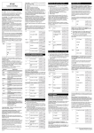
which correspond to the explicit description of all integer solutions:
Feasible solutions
Computed representation
y = 3x + 1
7
6
5
4
3
2
1
y = 3x + 1
6
5
y=x-2
1
2
3
4
5
6
7
1111111111111
0000000000000
0000000000000
1111111111111
0000000000000
1111111111111
0000000000000
1111111111111
0000000000000
1111111111111
0000000000000
1111111111111
0000000000000
1111111111111
0000000000000
1111111111111
0000000000000
1111111111111
0000000000000
1111111111111
0000000000000
1111111111111
0000000000000
1111111111111
0000000000000
1111111111111
0000000000000
1111111111111
0000000000000
1111111111111
0000000000000
1111111111111
0000000000000
1111111111111
0000000000000
1111111111111
0000000000000
1111111111111
0000000000000
1111111111111
7
111111111111111111111111111
000000000000000000000000000
111111111111111111111111111
000000000000000000000000000
111111111111111111111111111
000000000000000000000000000
111111111111111111111111111
000000000000000000000000000
111111111111111111111111111
000000000000000000000000000
111111111111111111111111111
000000000000000000000000000
111111111111111111111111111
000000000000000000000000000
111111111111111111111111111
000000000000000000000000000
111111111111111111111111111
000000000000000000000000000
111111111111111111111111111
000000000000000000000000000
111111111111111111111111111
000000000000000000000000000
111111111111111111111111111
000000000000000000000000000
111111111111111111111111111
000000000000000000000000000
111111111111111111111111111
000000000000000000000000000
111111111111111111111111111
000000000000000000000000000
111111111111111111111111111
000000000000000000000000000
111111111111111111111111111
000000000000000000000000000
111111111111111111111111111
000000000000000000000000000
111111111111111111111111111
000000000000000000000000000
111111111111111111111111111
000000000000000000000000000
111111111111111111111111111
000000000000000000000000000
111111111111111111111111111
000000000000000000000000000
111111111111111111111111111
000000000000000000000000000
000000000000000000000000000
111111111111111111111111111
111111111111111111111111111
000000000000000000000000000
111111111111111111111111111
000000000000000000000000000
111111111111111111111111111
000000000000000000000000000
111111111111111111111111111
000000000000000000000000000
000000000000000000000000000
111111111111111111111111111
000000000000000000000000000
111111111111111111111111111
111111111111111111111111111
000000000000000000000000000
111111111111111111111111111
000000000000000000000000000
111111111111111111111111111
000000000000000000000000000
000000000000000000000000000
111111111111111111111111111
000000000000000000000000000
111111111111111111111111111
111111111111111111111111111
000000000000000000000000000
111111111111111111111111111
000000000000000000000000000
111111111111111111111111111
000000000000000000000000000
111111111111111111111111111
000000000000000000000000000
000000000000000000000000000
111111111111111111111111111
111111111111111111111111111
000000000000000000000000000
111111111111111111111111111
000000000000000000000000000
111111111111111111111111111
000000000000000000000000000
111111111111111111111111111
000000000000000000000000000
000000000000000000000000000
111111111111111111111111111
000000000000000000000000000
111111111111111111111111111
111111111111111111111111111
000000000000000000000000000
111111111111111111111111111
000000000000000000000000000
111111111111111111111111111
000000000000000000000000000
000000000000000000000000000
111111111111111111111111111
000000000000000000000000000
111111111111111111111111111
111111111111111111111111111
000000000000000000000000000
111111111111111111111111111
000000000000000000000000000
y=x-2
4
3
2
1
8
9
1
2
3
4
5
6
7
8
9
1
2
0
1
1
1
1
,
,
,
+ monoid
,
,
.
0
0
1
1
1
2
3
Note that in the pictures above, we are only interested in the lattice points inside
the colored regions! The full regions are colored only for the purpose of visualizing
the covering of all feasible integer solutions by finitely many shifted copies of the
monoid
1
1
1
monoid
,
,
.
1
2
3
1.2. Brief tutorial
1.2.2
10
Solving linear systems over Q with qsolve
qsolve solves linear systems over Q; however, note that it only supports homogeneous linear systems, that is, systems with b = 0.
./qsolve system
This call creates files
system.qhom
system.qfree
To solve an inhomogeneous system Ax = b, x ≥ 0, you (still) need to do some work
yourself:
1. Solve system Ax − bu = 0, x ≥ 0, u ≥ 0 using qsolve.
2. Keep those solutions with u = 0. (These generate the recession cone (of unbounded directions).
3. Normalize those solutions with u > 0 to have u = 1 (by dividing the vector
by u). Be aware that this could create rational numbers.
4. Drop the u-component.
Any solution to Ax = b, x ≥ 0 can then be obtained by adding one solution from 3.
to a nonnegative linear combination of solutions from 2.
1.2.3
Computing extreme rays and Hilbert bases
In this example you learn about the functions rays and hilbert. (They are convenient versions of qsolve and zsolve for particular cases.)
Let us consider the set of magic 3 × 3 squares with non-negative real entries, that
is, the set of all 3 × 3 arrays with non-negative real entries whose row sums, column
sums, and main diagonal sums all add up to the same number, the magic constant
of the square.
Chapter 1. Beginner’s guide
11
Clearly, addition of two magic squares gives another magic square, as well as does
multiplication of a magic square by a non-negative number. Therefore, we may talk
about the cone of magic 3 × 3 squares. In fact, this cone is a pointed rational
polyhedral cone described by the linear system
x11 + x12 + x13 = x21 + x22 + x23
= x31 + x32 + x33
= x11 + x21 + x31
= x12 + x22 + x32
= x13 + x23 + x33
= x11 + x22 + x33
= x31 + x22 + x13
xij ≥ 0,
Bringing all xij to the left-hand side of
this linear system is

1 1 1 −1

 1 1 1
0

 0 1 1 −1


A3×3 =  1 0 1
0

 1 1 0
0

 0 1 1
0

1 1 0
0
for all i, j = 1, 2, 3.
these equations, the matrix A3×3 defining

−1 −1
0
0
0

0
0 −1 −1 −1 

0
0 −1
0
0 


−1
0
0 −1
0 .

0 −1
0
0 −1 

−1
0
0
0 −1 

−1
0 −1
0
0
Below, we will deal with the more interesting case of integer magic squares. For the
moment, however, we wish to compute the extreme rays of the magic square cone
{z : A3×3 z = 0, z ≥ 0}.
In order to call the function rays, we only have to create one file, say magic3x3.mat,
in which we specify the problem matrix A3×3 . The remaining data is set by default to
1.2. Brief tutorial
12
”equations only”, to ”homogeneous system”, and to ”all variables are non-negative”.
Note that we are allowed to change these defaults (except homogeneity) by specifying
data in magic3x3.rel and magic3x3.sign
magic3x3.mat
7 9
1 1 1 −1
1 1 1
0
0 1 1 −1
1 0 1
0
1 1 0
0
0 1 1
0
1 1 0
0
−1 −1
0
0
0
0
0 −1 −1 −1
0
0 −1
0
0
−1
0
0 −1
0
0 −1
0
0 −1
−1
0
0
0 −1
−1
0 −1
0
0
Now we call
./rays magic3x3
which creates the single file
magic3x3.ray
4 9
0 2 1 2
1 2 0 0
2 0 1 0
1 0 2 2
1
1
1
1
0
2
2
0
1
2
1
0
0
0
2
2
2
1
0
1
that corresponds to the four extremal rays of the 3 × 3 magic square cone:
0
2
1
1
2
0
2
0
1
1
0
2
2
1
0
0
1
2
0
1
2
2
1
0
1
0
2
2
0
1
1
2
0
0
2
1
Every magic 3 × 3 square is a non-negative linear combination of these four magic
squares.
If we turn now to integer magic squares, we are looking for a Hilbert basis of the
3 × 3 magic square cone. As the default settings for hilbert are the same as for
rays, we can use the same input file
Chapter 1. Beginner’s guide
13
magic3x3.mat
7 9
1 1 1 −1
1 1 1
0
0 1 1 −1
1 0 1
0
1 1 0
0
0 1 1
0
1 1 0
0
−1 −1
0
0
0
0
0 −1 −1 −1
0
0 −1
0
0
−1
0
0 −1
0
0 −1
0
0 −1
−1
0
0
0 −1
−1
0 −1
0
0
for this computation. However, to compute the Hilbert basis, we call
./hilbert magic3x3
which creates the single output file
magic3x3.hil
5 9
0 2 1 2
1 2 0 0
2 0 1 0
1 0 2 2
1 1 1 1
1
1
1
1
1
0
2
2
0
1
1
2
1
0
1
0
0
2
2
1
2
1
0
1
1
that corresponds to the five elements in the minimal Hilbert basis of the 3 × 3 magic
square cone:
0
2
1
1
2
0
2
0
1
1
0
2
2
1
0
0
1
2
0
1
2
2
1
0
1
0
2
2
0
1
1
2
0
0
2
1
1
1
1
1
1
1
1
1
1
1.2. Brief tutorial
14
Every integer magic 3 × 3 square is a non-negative integer linear combination of
these five integer magic squares. Note that the all-1 square is in the interior of the
magic square cone.
See [2, section 3.8] or [6] for details on the algorithm implemented.
1.2.4
Computing circuits and Graver bases
In this example you learn about the functions graver, ppi, and circuits.
As an example of a Graver basis computation, let us compute the primitive partition
identities of order n = 4. Before we do the simple computation, let us explain what
a primitive partition identity is.
A partition identity is any identity of the form
a1 + . . . + ak = b1 + . . . + bl
with (generally not distinct) integer numbers 0 < ai , bj ≤ n. A partition identity is
called primitive if no proper subidentity exists.
For example,
1+2+3=2+2+2
is a partition identity which is not primitive, since it contains the subidentity
1+3=2+2
which is in fact primitive.
The description of the primitive partition identities for fixed n, however, is exactly
the description of the Graver basis of the matrix
An = 1 2 3 . . . n .
Let us finally do the computation for n = 3. We create an input file ppi3 for 4ti2
which looks as follows:
ppi3.mat
1 3
1 2 3
Chapter 1. Beginner’s guide
15
and call
./graver ppi3
This call will create an output file ppi3.gra that looks like:
ppi3.gra
5
3
3
0 −1
2 −1
0
0
3 −2
1
1 −1
1 −2
1
Thus, there are 5 primitive partition identities of order n = 3:
1+1+1 = 3
1+1 = 2
2+2+2 = 3+3
1+2 = 3
1+3 = 2+2
You may try and compute the primitive partition identities for bigger n, say n = 17,
20, or 23. Be aware, especially the latter two problems take a long, long time. What
is the biggest n for which you can compute the primitive partition identities of order
n on your machine within one hour?
Due to the very special structure of the matrix, there are algorithmic speed-ups
[4, 10, 13]. The currently fastest algorithm to compute primitive partition identities
is implemented in the function ppi of 4ti2. Try running
./ppi 17
which creates two files ppi17.mat (so we do not really have to create this file ourselves) and the file ppi17.gra containing the desired identities. Compare this running time with the time taken by
1.2. Brief tutorial
16
./graver ppi17
Do you notice the speed-up?
Let us now turn to the question of determining the support-minimal partition identities. This, in fact, is the question of computing the circuits of the matrix
An = 1 2 3 . . . n .
We use the same input file
ppi3.mat
1 3
1 2 3
as above and call
./circuits ppi3
This call will create an output file ppi3.cir that looks like:
ppi3.cir
3
3
3
0 −1
2 −1
0
0
3 −2
Thus, there are 3 support-minimal partition identities of order n = 3:
1+1+1 = 3
1+1 = 2
2+2+2 = 3+3
Note that support-minimal partition identities are primitive, since the circuits of a
matrix are contained in the Graver basis of this matrix.
See the book [2, section 3.8], or Hemmecke [7] for details on the algorithm implemented.
Chapter 1. Beginner’s guide
1.2.5
17
Integer programming and toric Gr¨
obner bases
In this example you learn about the functions minimize, groebner, and normalform.
The following neat example is based on the example presented in [12]. Let us assume
that we want to give change worth 99 cents using only pennies (1ct), nickels (5ct),
dimes (10ct), and quarters (25ct). Clearly,
4 · 1 + 4 · 5 + 0 · 10 + 3 · 25 = 99
would be one way to do it. Is this there another choice of 11 coins that sums up to
99ct but uses fewer nickels and quarters (in total)? In other words, we would like to
solve
min{x2 + x4 : x1 + x2 + x3 + x4 = 11, x1 + 5x2 + 10x3 + 25x4 = 99, x1 , x2 , x3 , x4 ∈ Z+ }
Let us set up the problem in 4ti2.
4coins.mat
2 4
1 1 1 1
1 5 10 25
4coins.zsol
1 4
4 4 0 3
4coins.sign
1 4
1 1 1 1
4coins.cost
1 4
0 1 0 1
Note that we do not have to specify a relations file 4coins.rel, since already by
default all relations are assumed to be equations. Now we simply call
./minimize 4coins
which creates the single output file
4coins.min
1 4
4 1 4 2
From this, we conclude that
4 · 1 + 1 · 5 + 4 · 10 + 2 · 25 = 99
is an optimal choice, using only 3 instead of 7 nickels and quarters.
1.2. Brief tutorial
18
Remark. Earlier versions of 4ti2 allowed to specify the right-hand side vector in
a file called 4coins.rhs, instead of giving a solution in 4coins.zsol. This is no
longer supported.
Since we already know a feasible solution, there is another way we might attack this
problem, namely via toric Gr¨obner bases. (See [2, Chapter 11] for an introduction to
toric ideals and their Gr¨obner bases, and also their generalizations, lattice ideals.)
For this, we first need to specify the matrix A and the cost vector c in the two files
4coins.mat and 4coins.cost:
4coins.mat
2 4
1 1 1 1
1 5 10 25
4coins.cost
1 4
0 1 0 1
Then we compute the Gr¨obner basis of the toric ideal
IA = hxu − xv : Au = Av, u, v ∈ Z4+ i
with respect to a term ordering ≺ compatible with c, that is, c| v < c| u implies
xv ≺ xu . This toric Gr¨obner basis is computed by
./groebner 4coins
and gives the output file
4coins.gro
Remark. Many algorithm options are available and can be selected by commandline options of groebner, see section 3.5. As reference to the algorithms we recommend the book [2, section 11.4] or Hemmecke and Malkin [8], as well as Bigatti,
LaScala, and Robbiano [1], Gebauer and M¨oller [3], and Ho¸sten and Sturmfels [9].
Since runnning times of the various algorithms are hard to predict, it may for some
hard problems make sense to start several computations in parallel, each with different algorithms.
Then we specify our feasible solution in
Chapter 1. Beginner’s guide
19
4coins.feas
1 4
4 4 0 3
and call
./normalform 4coins
to produce the file
4coins.nf
1 4
4 1 4 2
that also contains the desired optimal solution.
Remark. We could also specify a list of feasible solutions in 4coins.feas. Then
the call
./normalform 4coins
creates a file 4coins.nf containing the minima to the corresponding integer programs. (If z0 is a feasible solution, the corresponding integer program is defined by
putting the right-hand side to Az0 .)
1.2.6
Markov Bases in Statistics
In this example you learn about the functions markov and genmodel.
Let us consider the following 4 × 4 table of non-negative integer numbers together
with all row and column sums.


11 23 34 3
71
 4 15 12 11  42




 17 2 3 25  47
16 12 22 7
57
48 52 71 46
1.2. Brief tutorial
20
In statistics, one wishes to sample among arrays that have fixed counts, say fixed row
and column sums. In order to sample, one needs a set of moves that, in particular,
do not change the counts when added to the current table. Clearly, these moves
must have counts 0 and thus quite naturally lead us to the toric ideal
IA = hxu − xv : Au = Av, u, v ∈ Z16
+ i,
where








A=






1
0
0
0
1
0
0
0
1
0
0
0
0
1
0
0
1
0
0
0
0
0
1
0
1
0
0
0
0
0
0
1
0
1
0
0
1
0
0
0
0
1
0
0
0
1
0
0
0
1
0
0
0
0
1
0
0
1
0
0
0
0
0
1
0
0
1
0
1
0
0
0
0
0
1
0
0
1
0
0
0
0
1
0
0
0
1
0
0
0
1
0
0
0
0
1
0
0
0
1
1
0
0
0
0
0
0
1
0
1
0
0
0
0
0
1
0
0
1
0
0
0
0
1
0
0
0
1








.






It turns out that for any set of fixed counts, a (minimal) Markov basis is given by
a minimal generating set of this toric ideal. Note that a Markov basis connects all
non-negative tables with these counts in the sense that for any two non-negative
tables T1 and T2 with these counts, there is a sequence of non-negative tables T1 =
S0 , . . . , SN = T2 with the same counts as T1 and T2 and such that Si − Si−1 or
Si−1 − Si is in the Markov basis for i = 1, . . . , N .
For two-way tables the situation is still very simple as our computations with 4 × 4
tables will now demonstrate. Write the matrix that defines our toric ideal in the file
4x4.mat:
4x4.mat
8 16
1 1
0 0
0 0
0 0
1 0
0 1
0 0
0 0
1
0
0
0
0
0
1
0
1
0
0
0
0
0
0
1
0
1
0
0
1
0
0
0
0
1
0
0
0
1
0
0
0
1
0
0
0
0
1
0
0
1
0
0
0
0
0
1
0
0
1
0
1
0
0
0
0
0
1
0
0
1
0
0
0
0
1
0
0
0
1
0
0
0
1
0
0
0
0
1
0
0
0
1
1
0
0
0
0
0
0
1
0
1
0
0
0
0
0
1
0
0
1
0
0
0
0
1
0
0
0
1
Chapter 1. Beginner’s guide
21
Let us compute the Markov basis via the call
./markov 4x4
which creates a single output file 4x4.mar containing the 36 Markov basis elements.
Up to symmetry (swapping rows or columns), the Markov basis consists of the single
move


1 −1 0 0
 −1
1 0 0 



.
 0
0 0 0 
0
0 0 0
In fact, this elementary move is (up to symmetry) the only representative of the
minimal Markov moves for arbitrary m × n tables using row and column counts.
Creating the matrices for statistical models may be pretty cumbersome. 4ti2 provides a litte function, genmodel, that helps the user with creating matrices for
hierarchical models defined by a complex.
The m × n tables problem above corresponds to the complex {{1}, {2}} on two
nodes with levels m and n, respectively. Let us encode the complex for 3 × 6 tables
with 1-marginals (row and column sums) in 3x6.mod.
3x6.mod
3
3 6
2
1 1
1 2
and call
./genmodel 3x6
to produce the desired matrix file 3x6.mat.
The encoding of the complex should be obvious from the example: first we state the
number of nodes and their levels, then we give the number of maximal faces. Finally,
1.2. Brief tutorial
22
we list each maximal face by first specifying the number of nodes on it and then by
listing these nodes.
Thus, a 3 × 4 × 6 table with 2-marginals (that is, again only counts along coordinate
axes) corresponds to the complex {{(1, 2)}, {(2, 3)}, {(3, 1)}} on 3 nodes with levels
3, 4, and 6, respectively. Thus, its encoding is in 4ti2 would look like:
3x4x6.mod
3
3 4 6
3
2 1 2
2 2 3
2 3 1
A binary model on the bipartite graph K2,3 then reads as
k2 3.mod
5
2 2 2 2 2
6
2 1 3
2 1 4
2 1 5
2 2 3
2 2 4
2 2 5
Chapter 2
Advanced guide
In this part, we deal with several more advanced problem specifications in 4ti2.
First we introduce affine systems and their encodings. In fact, affine systems are
the basic objects used in 4ti2, since every linear system is transformed into an
affine system. However, in the integer situation, it is not always possible to transform an affine system back into a linear system without adding variables or modulo
constraints.
2.1
Affine systems and their encodings
Let a + LZ be an “integer linear affine space” given by the vector a ∈ Zn and
by generators for the lattice LZ ⊆ Zn . We wish to find a finite sign-compatible
description for the set of all (integer) vectors x ∈ a + LZ .
As an example, let consider the linear space LR and the lattice LZ both spanned
by the two vectors (1, −2, 1, 0) and (2, −3, −0, 1). Moreover, consider the signconstraints (1, 2, 2, 0). Thus, we are looking for a finite explicit sign-compatible
description for all x that can be written as



x=


1
2
−2 −3 

 λ,
1
0 
0
1
23
2.1. Affine systems and their encodings
24
with λ ∈ R2 and λ ∈ Z2 , respectively.
In order to solve this affine system using zsolve, we create the following input files
to encode the affine system:
affine.lat
2
4
1 −1 1 0
2 −3 0 1
affine.sign
1 4
1 2 2 0
and then call
./zsolve affine
This creates the files affine.zhom and affine.zinhom.
Chapter 3
Command-line reference
3.1
circuits
Usage: circuits [options] PROJECT
Computes the circuits of a cone.
Input Files:
PROJECT.mat
PROJECT.sign
PROJECT.rel
Output Files:
PROJECT.cir
PROJECT.qfree
A matrix (compulsory).
The sign constraints of the variables (’1’ means
non-negative, ’0’ means a free variable, and ’2’ means
both non-negative and non-positive).
It is optional, and the default is both.
The relations on the matrix rows (’<’,’>’,’=’).
It is optional and the default is all ’=’.
The mat must be given with this file.
The circuits of the cone.
A basis for the linear subspace of the cone.
If this file does not exist then the linear subspace
is trivial.
Options:
-p, --precision=PREC
Select PREC as the integer arithmetic precision.
25
3.1. circuits
-m, --mat
-s, --support
-o, --order=ORDERING
-f, --output-freq=n
-q, --quiet
-h, --help
26
PREC is one of the following: ‘64’ (default),
‘32’, and ‘arbitrary’ (only ‘arb‘ is needed).
Use the Matrix algorithm (default for 32 and 64).
Use the Support algorithm (default for arbitrary).
Set ORDERING as the ordering in which the columns
are chosen. The possible orderings are ‘maxinter’,
‘minindex’, ‘maxcutoff’ (default), and ‘mincutoff’.
Set the frequency of output (default is 1000).
Do not output anything to the screen.
Display this help and exit.
Chapter 3. Command-line reference
3.2
27
genmodel
usage: genmodel [--options] FILENAME
Computes the problem matrix corresponding to graphical statistical models
given by a simplicial complex and levels on the nodes.
Options:
-q, --quiet No output is written to the screen
Input file:
FILENAME.mod
Simplicial complex and levels on the nodes
Output file:
FILENAME.mat
Matrix file
Example: Consider the problem of 3x3x3 tables
are given by K_3 as the simplicial complex on
of 3 on each node. In ’333.mod’ write:
3
3 3 3
3
2 1 2
2 2 3
2 3 1
Calling ’genmodel 333’ produces the following
27 27
1 0 0 0 0 0 0 0 0 1 0 0 0 0 0 0 0 0 1 0 0 0 0
0 1 0 0 0 0 0 0 0 0 1 0 0 0 0 0 0 0 0 1 0 0 0
[...]
1 0 0 1 0 0 1 0 0 0 0 0 0 0 0 0 0 0 0 0 0 0 0
0 1 0 0 1 0 0 1 0 0 0 0 0 0 0 0 0 0 0 0 0 0 0
0 0 1 0 0 1 0 0 1 0 0 0 0 0 0 0 0 0 0 0 0 0 0
[...]
1 1 1 0 0 0 0 0 0 0 0 0 0 0 0 0 0 0 0 0 0 0 0
0 0 0 1 1 1 0 0 0 0 0 0 0 0 0 0 0 0 0 0 0 0 0
with 2-marginals. These
3 nodes and with levels
file ’333.mat’:
0 0 0 0
0 0 0 0
0 0 0 0
0 0 0 0
0 0 0 0
0 0 0 0
0 0 0 0
3.2. genmodel
[...]
28
Chapter 3. Command-line reference
3.3
29
gensymm
usage: gensymm [--options] A B C D FILENAME
Computes the generators for the symmetry group acting on 4-way tables
with 3-marginals. By putting one side length to 1, this includes
3-way tables with 2-marginals.
Options:
-q, --quiet
No output is written to the screen
Output file:
FILENAME.sym
generators for the symmetry group
Example: Consider the problem of 3x3x3 tables with 2-marginals. Calling
gensymm 3 3 3 1 333
produces the file ’333.sym’ containing the following lines.
9 27
10 11 12 13 14 15
10 11 12 13 14 15
4 5 6 7 8 9 1 2 3
4 5 6 1 2 3 7 8 9
2 3 1 5 6 4 8 9 7
2 1 3 5 4 6 8 7 9
1 2 3 10 11 12 19
1 10 19 4 13 22 7
1 4 7 2 5 8 3 6 9
16
16
13
13
11
11
20
16
10
17
17
14
14
12
10
21
25
13
18 19 20 21 22 23 24
18 1 2 3 4 5 6 7 8 9
15 16 17 18 10 11 12
15 10 11 12 16 17 18
10 14 15 13 17 18 16
12 14 13 15 17 16 18
4 5 6 13 14 15 22 23
2 11 20 5 14 23 8 17
16 11 14 17 12 15 18
25
19
22
22
20
20
24
26
19
26 27 1 2 3 4 5 6
20 21 22 23 24 25
23 24 25 26 27 19
23 24 19 20 21 25
21 19 23 24 22 26
19 21 23 22 24 26
7 8 9 16 17 18 25
3 12 21 6 15 24 9
22 25 20 23 26 21
7 8 9
26 27
20 21
26 27
27 25
25 27
26 27
18 27
24 27
3.4. graver
3.4
30
graver
Usage: graver [options] PROJECT
Computes the Graver basis of a matrix or a given lattice.
Basic options:
-p PREC, --precision=PREC
-m, --maxnorm
-b [FREQ], --backup[=FREQ]
-r, --resume
-h, --help
--version
Output options:
-q, --quiet
-u, --update[=1]
-uu, --update=2
-v, --verbose[=1]
-vv, --verbose=2
-vvv, --verbose=3
Use precision (32, 64, gmp). Default is 32 bit
Write vectors with maximum norm to PROJECT.maxnorm
Frequently backup status to PROJECT.backup
Resume from backup file PROJECT.backup
Display this help
Display version information
Quiet mode
Updated output on console (default)
More verbose updated output on console
Output once every variable computation
Output once every norm sum computation
Output once every norm computation
Logging options:
-n, --log=0
Disable logging (default)
-l, --log[=1] Log once every variable computation to PROJECT.log
-ll, --log=2
Log once every norm sum computation to PROJECT.log
-lll, --log=3 Log once every norm computation to PROJECT.log
Input files:
PROJECT.mat
PROJECT.lat
PROJECT.sign
PROJECT.lb
PROJECT.ub
Backup files:
Matrix
Lattice basis (can be provided instead of matrix)
Sign of columns (optional)
Lower bounds of columns (optional)
Upper bounds of columns (optional)
Chapter 3. Command-line reference
PROJECT.backup Backup file
PROJECT.backup~ Temporary backup file
(if it exists, it may be newer than PROJECT.backup)
Output files:
PROJECT.gra
Graver basis
PROJECT.zfree
Free part of the solution
PROJECT.maxnorm Vectors with maximum norm (if -m, --maxnorm is in use)
31
3.5. groebner
3.5
32
groebner
Usage: groebner [options] PROJECT
Computes a Groebner basis of the toric ideal of a matrix,
or, more general, of the lattice ideal of a lattice.
Input Files:
PROJECT.mat
PROJECT.lat
PROJECT.cost
A matrix (optional if lattice basis is given).
A lattice basis (optional if matrix is given).
The cost matrix, which determines the term ordering
(optional, default is degrevlex).
Ties are broken with degrevlex.
PROJECT.sign
The sign constraints of the variables (’1’ means
non-negative and ’0’ means a free variable).
It is optional, and the default is all non-negative.
PROJECT.mar
The Markov basis/generating set of the lattice (optional).
PROJECT.weights
The weight vectors used for truncation (optional).
PROJECT.weights.max The maximum weights used for truncation.
This file is needed when PROJECT.weights exists.
PROJECT.zsol
An integer solution to specify a fiber (optional).
The integer solution is used for truncation.
Output Files:
PROJECT.gro
The Groebner basis of the lattice.
Options:
-p, --precision=PREC
-a, --algorithm=ALG
-g, --generation=ALG
Select PREC as the integer arithmetic precision.
PREC is one of the following: ‘64’ (default),
‘32’, and ‘arbitrary’ (only ‘arb‘ is needed).
Select ALG as the completion procedure for
computing Groebner bases. ALG is one of
‘fifo’, ‘weighted’, or ’unbounded.’
Select ALG as the procedure for computing
a generating set or Markov basis. ALG is
one of ‘hybrid’ (default), ‘project-and-lift’,
‘max-min’, or ’saturation’.
Chapter 3. Command-line reference
-t, --truncation=TRUNC
-m, --minimal=STATE
-r, --auto-reduce-freq=n
-f, --output-freq=n
-q, --quiet
-h, --help
33
Set TRUNC as the truncation method. TRUNC is
of the following: ‘ip’, ‘lp’, ‘weight’ (default),
or ‘none’. Only relevant if ‘zsol’ is given.
If STATE is ‘yes’ (default), then 4ti2 will
compute a minimal Markov basis. If STATE is
’no’, then the Markov basis will not
necessarily be minimal.
Set the frequency of auto reduction.
(default is 2500).
Set the frequency of output (default is 1000).
Do not output anything to the screen.
Display this help and exit.
3.6. hilbert
3.6
34
hilbert
Usage: hilbert [options] PROJECT
Computes the Hilbert basis of a matrix or a given lattice.
Basic options:
-p PREC, --precision=PREC
-m, --maxnorm
-b [FREQ], --backup[=FREQ]
-r, --resume
-h, --help
--version
Output options:
-q, --quiet
-u, --update[=1]
-uu, --update=2
-v, --verbose[=1]
-vv, --verbose=2
-vvv, --verbose=3
Use precision (32, 64, gmp). Default is 32 bit
Write vectors with maximum norm to PROJECT.maxnorm
Frequently backup status to PROJECT.backup
Resume from backup file PROJECT.backup
Display this help
Display version information
Quiet mode
Updated output on console (default)
More verbose updated output on console
Output once every variable computation
Output once every norm sum computation
Output once every norm computation
Logging options:
-n, --log=0
Disable logging (default)
-l, --log[=1] Log once every variable computation to PROJECT.log
-ll, --log=2
Log once every norm sum computation to PROJECT.log
-lll, --log=3 Log once every norm computation to PROJECT.log
Input files:
PROJECT.mat
PROJECT.lat
PROJECT.rel
PROJECT.sign
PROJECT.ub
Backup files:
Matrix
Lattice basis (can be provided instead of matrix)
Relations (<, >, =)
Sign of columns (optional)
Upper bounds of columns (optional)
Chapter 3. Command-line reference
PROJECT.backup Backup file
PROJECT.backup~ Temporary backup file
(if it exists, it may be newer than PROJECT.backup)
Output files:
PROJECT.hil
Hilbert basis
PROJECT.zfree
Free part of the solution
PROJECT.maxnorm Vectors with maximum norm (if -m, --maxnorm is in use)
35
3.7. markov
3.7
36
markov
Usage: markov [options] PROJECT
Computes a Markov basis (generating set) of the toric ideal
of a matrix or, more general, of the lattice ideal of a lattice.
Input Files:
PROJECT
PROJECT.lat
PROJECT.sign
A matrix (optional only if lattice basis is given).
A lattice basis (optional only if matrix is given).
The sign constraints of the variables (’1’ means
non-negative and ’0’ means a free variable).
It is optional, and the default is all non-negative.
PROJECT.weights
The weight vectors used for truncation (optional).
PROJECT.weights.max The maximum weights used for truncation.
This file is needed when PROJECT.weights exists.
PROJECT.zsol
An integer solution to specify a fiber (optional).
The integer solution is used for truncation.
Output Files:
PROJECT.mar
The Markov basis/generating set of the lattice.
Options:
-p, --precision=PREC
Select PREC as the integer arithmetic precision.
PREC is one of the following: ‘64’ (default),
‘32’, and ‘arbitrary’ (only ‘arb‘ is needed).
-a, --algorithm=ALG
Select ALG as the completion procedure for
computing Groebner bases. ALG is one of
‘fifo’, ‘weighted’, or ’unbounded.’
-g, --generation=ALG
Select ALG as the procedure for computing
a generating set or Markov basis. ALG is
one of ‘hybrid’ (default), ‘project-and-lift’,
‘max-min’, or ’saturation’.
-t, --truncation=TRUNC
Set TRUNC as the truncation method. TRUNC is
of the following: ‘ip’, ‘lp’, ‘weight’ (default),
or ‘none’. Only relevant if ‘zsol’ is given.
-m, --minimal=STATE
If STATE is ‘yes’ (default), then 4ti2 will
compute a minimal Markov basis. If STATE is
Chapter 3. Command-line reference
-r, --auto-reduce-freq=n
-f, --output-freq=n
-q, --quiet
-h, --help
37
’no’, then the Markov basis will not
necessarily be minimal.
Set the frequency of auto reduction.
(default is 2500).
Set the frequency of output (default is 1000).
Do not output anything to the screen.
Display this help and exit.
3.8. minimize
3.8
38
minimize
Usage: minimize [options] PROJECT
Computes the minimal solution of an integer linear program
or, more general, a lattice program, using a Groebner basis.
Input Files:
PROJECT.mat
PROJECT.lat
PROJECT.cost
PROJECT.zsol
PROJECT.sign
Output Files:
PROJECT.min
A matrix (optional only if lattice basis is given).
A lattice basis (optional only if matrix is given).
The cost vector. Exactly one vector allowed.
An integer solution to specify a fiber (needed).
The sign constraints of the variables (’1’ means
non-negative and ’0’ means a free variable).
It is optional, and the default is all non-negative.
The minimal solution for the given fiber.
Options:
-p, --precision=PREC
-a, --algorithm=ALG
-t, --truncation=TRUNC
-r, --auto-reduce-freq=n
-f, --output-freq=n
-q, --quiet
-h, --help
Select PREC as the integer arithmetic precision.
PREC is one of the following: ‘64’ (default),
‘32’, and ‘arbitrary’ (only ‘arb‘ is needed).
Select ALG as the completion procedure for
computing Groebner bases. ALG is one of
‘fifo’, ‘weighted’, or ’unbounded.’
Set TRUNC as the truncation method. TRUNC is
of the following: ‘ip’, ‘lp’, ‘weight’ (default),
or ‘none’. Only relevant if ‘zsol’ is given.
Set the frequency of auto reduction.
(default is 2500).
Set the frequency of output (default is 1000).
Do not output anything to the screen.
Display this help and exit.
Chapter 3. Command-line reference
3.9
39
normalform
Usage: normalform [options] PROJECT
Computes the normal form of a list of feasible points.
Input Files:
PROJECT.mat
PROJECT.lat
PROJECT.gro
PROJECT.cost
PROJECT.feas
PROJECT.sign
Output Files:
PROJECT.nf
A matrix (optional if lattice basis is given).
A lattice basis (optional if matrix is given).
The Groebner basis of the lattice (needed).
The cost matrix (optional, default is degrevlex).
Ties are broken with degrevlex.
An list of integer feasible solutions (needed).
The sign constraints of the variables (’1’ means
non-negative and ’0’ means a free variable).
It is optional, and the default is all non-negative.
The normal forms of the feasible solutions.
Options:
-p, --precision=PREC
-q, --quiet
-h, --help
Select PREC as the integer arithmetic precision.
PREC is one of the following: ‘64’ (default),
‘32’, and ‘arbitrary’ (only ‘arb‘ is needed).
Do not output anything to the screen.
Display this help and exit.
3.10. output
3.10
40
output
usage: output [--options] FILENAME.EXT
Transforms a 4ti2 matrix file to something else.
General options:
--quiet
No output is written to the screen.
Options that control what to output:
--binomials
Write vectors as binomials.
Use an optional input file
’FILENAME.EXT.vars’
to specify variable names.
--maple
Write vectors as Maple list.
This format is suitable also for
CoCoA, Mathematica, Macaulay2.
--0-1
Extract vectors with 0-1
components only.
--transpose
Transpose matrix and write it
in 4ti2 format.
--degree
Print 1-norms of all vectors.
--degree N
Extract all vectors of 1-norm
equal to N.
--degree N1 N2 Extract all vectors of 1-norm
between N1 and N2 (inclusive).
--support
Print supports of all vectors.
--support S
Extract all vectors of support
their output files:
FILENAME.EXT.bin
FILENAME.EXT.maple
FILENAME.EXT.0-1
FILENAME.EXT.tra
FILENAME.EXT.deg.N
FILENAME.EXT.deg.N1-N2
FILENAME.EXT.supp.S
Chapter 3. Command-line reference
41
size equal to S.
--support S1 S2
Extract all vectors of support
size between S1 and S2 (incl.)
FILENAME.EXT.supp.S1-S2
--positive
Extract positive parts of vectors.
Corresponds to leading terms of
binomials.
FILENAME.EXT.pos
--3way A B C
Write vectors as 3-way tables
of size A x B x C.
FILENAME.EXT.3way
--nonzero-at K Extract all vectors that have
nonzero K-th coordinate.
Undocumented or obscure options for experts:
--representatives
--dominated
Extract all non-dominated vectors
--maximal-non-dominated
--expand-representatives-to-full-orbits
--type T
--AxB
Computes a matrix-vector product.
--macaulay2
--mathematica
--cocoa
--sum
Print the sum of the columns.
--submatrix LISTFILENAME
--remove-column I
--remcol I
--stabilizer SYMMFILENAME
--fill-column
--add-column
--fix I1 ... IK
Extract fixed vectors,
that is, those vectors that
have x[i]=i for the given i.
--fox I1 ... IK
Extract relaxed fixed vectors.
FILENAME.EXT.nonzero.K
FILENAME.EXT.nondom
FILENAME.EXT.maxnondom
FILENAME.EXT.submat
FILENAME.EXT.remcol
FILENAME.EXT.remcol
FILENAME.EXT.stab
FILENAME.EXT.fil
FILENAME.EXT.addcol
FILENAME.EXT.fix
FILENAME.EXT.fox
3.10. output
--initial-forms
42
Extract initial forms.
(Call with FILENAME rather
than FILENAME.EXT. Reads
FILENAME.gro and
optionally FILENAME.cost and
FILENAME.vars.
FILENAME.ini
FILENAME.ini.bin
Examples:
’output --binomials file.gra’ writes the Graver basis elements as
binomials in ’file.gra.bin’.
’output --0-1 foo.gra’ extracts the 0-1 elements from the Graver basis
elements and writes them into ’foo.gra.0-1’.
Chapter 3. Command-line reference
3.11
43
ppi
usage: ppi [--binary-output] N
Computes the primitive partition identities, that is, the Graver basis of [1 2 3 ... N].
Options:
-b, --binary-output
Create a binary file ppiN.dat instead of text file ppiN.gra
3.12. qsolve
3.12
44
qsolve
Usage: qsolve [options] PROJECT
Computes a generator description of a cone.
Input Files:
PROJECT.mat
PROJECT.sign
PROJECT.rel
Output Files:
PROJECT.qhom
PROJECT.qfree
A matrix (compulsory).
The sign constraints of the variables (’1’ means
non-negative, ’0’ means a free variable, and ’2’ means
both non-negative and non-positive).
It is optional, and the default is all free.
The relations on the matrix rows (’<’,’>’,’=’).
It is optional and the default is all ’=’.
The mat must be given with this file.
The homogeneous generators of the linear system.
A basis for the linear subspace of the cone.
If this file does not exist then the linear subspace
is trivial.
Options:
-p, --precision=PREC
-m, --mat
-s, --support
-o, --order=ORDERING
-f, --output-freq=n
-q, --quiet
-h, --help
Select PREC as the integer arithmetic precision.
PREC is one of the following: ‘64’ (default),
‘32’, and ‘arbitrary’ (only ‘arb‘ is needed).
Use the Matrix algorithm (default for 32 and 64).
Use the Support algorithm (default for arbitrary).
Set ORDERING as the ordering in which the columns
are chosen. The possible orderings are ‘maxinter’,
‘minindex’, ‘maxcutoff’ (default), and ‘mincutoff’.
Set the frequency of output (default is 1000).
Do not output anything to the screen.
Display this help and exit.
Chapter 3. Command-line reference
3.13
45
rays
Usage: rays [options] PROJECT
Computes the extreme rays of a cone.
Input Files:
PROJECT.mat
PROJECT.sign
PROJECT.rel
Output Files:
PROJECT.ray
PROJECT.qfree
A matrix (compulsory).
The sign constraints of the variables (’1’ means
non-negative, ’0’ means a free variable, and ’2’ means
both non-negative and non-positive).
It is optional, and the default is all non-negative.
The relations on the matrix rows (’<’,’>’,’=’).
It is optional and the default is all ’=’.
The mat must be given with this file.
The extreme rays of the cone.
A basis for the linear subspace of the cone.
If this file does not exist then the linear subspace
is trivial.
Options:
-p, --precision=PREC
-m, --mat
-s, --support
-o, --order=ORDERING
-f, --output-freq=n
-q, --quiet
-h, --help
Select PREC as the integer arithmetic precision.
PREC is one of the following: ‘64’ (default),
‘32’, and ‘arbitrary’ (only ‘arb‘ is needed).
Use the Matrix algorithm (default for 32 and 64).
Use the Support algorithm (default for arbitrary).
Set ORDERING as the ordering in which the columns
are chosen. The possible orderings are ‘maxinter’,
‘minindex’, ‘maxcutoff’ (default), and ‘mincutoff’.
Set the frequency of output (default is 1000).
Do not output anything to the screen.
Display this help and exit.
3.14. walk
3.14
46
walk
Usage: walk [options] PROJECT
Computes the minimal solution of an integer linear program
or, more general, a lattice program using a Groebner basis.
Input Files:
PROJECT.mat
PROJECT.lat
PROJECT.gro.start
PROJECT.gro.cost
PROJECT.cost
PROJECT.zsol
PROJECT.sign
Output Files:
PROJECT.gro
A matrix (optional only if lattice basis is given).
A lattice basis (optional only if matrix is given).
The starting Groebner basis (needed).
The starting cost vector (optional, default is degrevlex).
Ties are broken with degrevlex.
The target cost vector (optional, default is degrevlex).
Ties are broken with degrevlex.
An integer solution to specify a fiber (needed).
The sign constraints of the variables (’1’ means
non-negative and ’0’ means a free variable).
It is optional, and the default is all non-negative.
The Groebner basis of the lattice.
Options:
-p, --precision=PREC
-t, --truncation=TRUNC
-f, --output-freq=n
-q, --quiet
-h, --help
Select PREC as the integer arithmetic precision.
PREC is one of the following: ‘64’ (default),
‘32’, and ‘arbitrary’ (only ‘arb‘ is needed).
Set TRUNC as the truncation method. TRUNC is
of the following: ‘ip’, ‘lp’, ‘weight’ (default),
or ‘none’. Only relevant if ‘zsol’ is given.
Set the frequency of output (default is 1000).
Do not output anything to the screen.
Display this help and exit.
Chapter 3. Command-line reference
3.15
47
zbasis
Usage: zbasis [options] PROJECT
Computes an integer lattice basis.
Input Files:
PROJECT
A matrix (needed).
Output Files:
PROJECT.lat
A lattice basis.
Options:
-p, --precision=PREC
Select PREC as the integer arithmetic precision.
PREC is one of the following: ‘64’ (default),
‘32’, and ‘arbitrary’ (only ‘arb‘ is needed).
-q, --quiet
Do not output anything to the screen.
-h, --help
Display this help and exit.
3.16. zsolve
3.16
48
zsolve
Usage: zsolve [options] PROJECT
Solves linear inequality and equation systems over the integers.
Basic options:
-p PREC, --precision=PREC
-m, --maxnorm
-b [FREQ], --backup[=FREQ]
-r, --resume
-h, --help
--version
Output options:
-q, --quiet
-u, --update[=1]
-uu, --update=2
-v, --verbose[=1]
-vv, --verbose=2
-vvv, --verbose=3
Use precision (32, 64, gmp). Default is 32 bit
Write vectors with maximum norm to PROJECT.maxnorm
Frequently backup status to PROJECT.backup
Resume from backup file PROJECT.backup
Display this help
Display version information
Quiet mode
Updated output on console (default)
More verbose updated output on console
Output once every variable computation
Output once every norm sum computation
Output once every norm computation
Logging options:
-n, --log=0
Disable logging (default)
-l, --log[=1] Log once every variable computation to PROJECT.log
-ll, --log=2
Log once every norm sum computation to PROJECT.log
-lll, --log=3 Log once every norm computation to PROJECT.log
Input files:
PROJECT.mat
PROJECT.lat
PROJECT.rhs
PROJECT.rel
PROJECT.sign
PROJECT.lb
PROJECT.ub
Matrix
Lattice basis (can be provided instead of matrix)
Right hand side
Relations (<, >, =)
Sign of columns (optional)
Lower bounds of columns (optional)
Upper bounds of columns (optional)
Chapter 3. Command-line reference
Backup files:
PROJECT.backup Backup file
PROJECT.backup~ Temporary backup file
(if it exists, it may be newer than PROJECT.backup)
Output files:
PROJECT.zinhom
PROJECT.zhom
PROJECT.zfree
PROJECT.maxnorm
Inhomogeneous part of the solution
Homogeneous part of the solution
Free part of the solution
Vectors with maximum norm (if -m, --maxnorm is in use)
49
3.16. zsolve
50
Chapter 4
4ti2 as a callable library
Some portions of 4ti2 can be used as a callable library to avoid I/O and process
overhead. It has a simple C API that closely mirrors the commands: qsolve, rays,
circuits, zsolve, hilbert, graver.
Depending on its configuration, 4ti2 builds and installs several libraries, either as
static or shared libraries, using libtool.
The functions equivalent to zsolve, hilbert, graver require the use of libzsolve.
The functions equivalent to qsolve, rays, circuits require the use of lib4ti2common
and, depending on the arithmetic precision requested, the use of lib4ti2int32,
lib4ti2int64, or lib4ti2gmp.
4.1
C API header file: 4ti2/4ti2.h
A single header file, <4ti2/4ti2.h>, provides the C API. It is reproduced below for
reference.
/*
4ti2 -- A software package for algebraic, geometric and combinatorial
problems on linear spaces.
Copyright(C) 2008 4ti2 team.
Main author(s): Peter Malkin
This program is free software; you can redistribute it and/or
modify it under the terms of the GNU General Public License
51
4.1. C API header file: 4ti2/4ti2.h
52
as published by the Free Software Foundation; either version 2
of the License, or(at your option) any later version.
This program is distributed in the hope that it will be useful,
but WITHOUT ANY WARRANTY; without even the implied warranty of
MERCHANTABILITY or FITNESS FOR A PARTICULAR PURPOSE. See the
GNU General Public License for more details.
You should have received a copy of the GNU General Public License
along with this program; if not, write to the Free Software
Foundation, Inc., 51 Franklin Street, Fifth Floor, Boston, MA 02110-1301, USA.
*/
#ifndef _4ti2_H
#define _4ti2_H
#include <inttypes.h>
#include "4ti2/4ti2_config.h"
#ifdef _4ti2_HAVE_GMP
#include <gmp.h>
#endif
#ifdef __cplusplus
extern "C"
{
#endif
// Enum representing the possible arithmetic precision settings available.
typedef enum { _4ti2_PREC_INT_32 = 32, _4ti2_PREC_INT_64 = 64, _4ti2_PREC_INT_ARB = 0 } _4ti2_precision;
// Enum representing values describing the constraints on a variable or row of the constraint matrix.
typedef enum { _4ti2_FR = 0, _4ti2_LB = 1, _4ti2_UB = -1, _4ti2_DB = 2, _4ti2_FX = 3 } _4ti2_constraint;
// Enum representing the exit status of an API call to 4ti2.
typedef enum { _4ti2_OK = 0, _4ti2_ERROR = 1 } _4ti2_status;
// 4ti2 data structures.
typedef struct _4ti2_state _4ti2_state;
typedef struct _4ti2_matrix _4ti2_matrix;
// Create a QSolve 4ti2 state object.
_4ti2_state* _4ti2_qsolve_create_state(_4ti2_precision prec);
// Create a QSolve 4ti2 rays object.
_4ti2_state* _4ti2_rays_create_state(_4ti2_precision prec);
// Create a QSolve 4ti2 circuits object.
_4ti2_state* _4ti2_circuits_create_state(_4ti2_precision prec);
// Create a ZSolve 4ti2 state object.
Chapter 4. 4ti2 as a callable library
53
_4ti2_state* _4ti2_zsolve_create_state(_4ti2_precision prec);
// Create a ZSolve 4ti2 state object.
_4ti2_state* _4ti2_hilbert_create_state(_4ti2_precision prec);
// Create a ZSolve 4ti2 state object.
_4ti2_state* _4ti2_graver_create_state(_4ti2_precision prec);
// Read in options for the 4ti2 state object.
// These options are exactly the same as the command line options without the project filename at the end.
// Note that argv[0] is ignored!
_4ti2_status _4ti2_state_set_options(_4ti2_state* state, int argc, char** argv);
#if 0
/* Implementation does not exist. --mkoeppe */
// Read in the state object from "project"
_4ti2_status _4ti2_state_read(_4ti2_state* state, const char* project);
// Write out the state object to "project"
_4ti2_status _4ti2_state_write(_4ti2_state* state, const char* project);
#endif
// Deletes a 4ti2 state object.
void _4ti2_state_delete(_4ti2_state* state);
// Runs the main algorithm of the 4ti2 state object.
_4ti2_status _4ti2_state_compute(_4ti2_state* state);
// Create a 4ti2 matrix. Previous matrix is deleted if it exists. Pointer is 0 if "name" is not valid.
_4ti2_status _4ti2_state_create_matrix(_4ti2_state* state, int num_rows, int num_cols, const char* name, _4ti2_matrix** mat
// Read a 4ti2 matrix from a file. Previous matrix is deleted if it exists. Returns 0 if "name" is not valid.
_4ti2_status _4ti2_state_read_matrix(_4ti2_state* state, const char* filename, const char* name, _4ti2_matrix** matrix);
// Get a 4ti2 matrix. Returns 0 if "name" is not valid or if matrix has not been created.
_4ti2_status _4ti2_state_get_matrix(_4ti2_state* state, const char* name, _4ti2_matrix** matrix);
// Returns the number of rows of the matrix.
int _4ti2_matrix_get_num_rows(const _4ti2_matrix*
matrix);
// Returns the number of columns of the matrix.
int _4ti2_matrix_get_num_cols(const _4ti2_matrix*
matrix);
// Write the 4ti2 matrix to stdout.
void _4ti2_matrix_write_to_stdout(const _4ti2_matrix*
matrix);
// Write the 4ti2 matrix to sterr.
void _4ti2_matrix_write_to_stderr(const _4ti2_matrix*
matrix);
// Write the 4ti2 matrix to the file called "filename".
void _4ti2_matrix_write_to_file(const _4ti2_matrix* matrix, const char* filename);
4.2. Example program: zsolve
// Operations on the matrix.
_4ti2_status _4ti2_matrix_set_entry_int32_t(_4ti2_matrix*
54
matrix, int r, int c, _4ti2_int32_t value);
_4ti2_status _4ti2_matrix_get_entry_int32_t(const _4ti2_matrix*
_4ti2_status _4ti2_matrix_set_entry_int64_t(_4ti2_matrix*
matrix, int r, int c, _4ti2_int64_t value);
_4ti2_status _4ti2_matrix_get_entry_int64_t(const _4ti2_matrix*
#ifdef _4ti2_HAVE_GMP
_4ti2_status _4ti2_matrix_set_entry_mpz_ptr(_4ti2_matrix*
matrix, int r, int c, _4ti2_int32_t* value);
matrix, int r, int c, _4ti2_int64_t* value);
matrix, int r, int c, mpz_ptr value);
_4ti2_status _4ti2_matrix_get_entry_mpz_ptr(const _4ti2_matrix*
#endif
matrix, int r, int c, mpz_ptr value);
#ifdef __cplusplus
} // extern "C"
#endif
#endif
4.2
Example program: zsolve
Example programs using the C API can be found in the source tree of 4ti2, in the
directories test/qsolve/api and test/zsolve/api.
Below we reproduce the example program test/zsolve/api/test zsolve api.cpp.
/*
4ti2 -- A software package for algebraic, geometric and combinatorial
problems on linear spaces.
Copyright (C) 2006 4ti2 team.
Main author(s): Peter Malkin.
This program is
modify it under
as published by
of the License,
free software; you can redistribute it and/or
the terms of the GNU General Public License
the Free Software Foundation; either version 2
or (at your option) any later version.
This program is distributed in the hope that it will be useful,
but WITHOUT ANY WARRANTY; without even the implied warranty of
MERCHANTABILITY or FITNESS FOR A PARTICULAR PURPOSE. See the
GNU General Public License for more details.
You should have received a copy of the GNU General Public License
along with this program; if not, write to the Free Software
Foundation, Inc., 51 Franklin Street, Fifth Floor, Boston, MA 02110-1301, USA.
Chapter 4. 4ti2 as a callable library
*/
#include "4ti2/4ti2.h"
int
main()
{
// Input data.
const int m = 4;
const int n = 3;
_4ti2_int64_t mat[m][n] = {
{ 2, 3, -6 },
{ 2, -1, -4 },
{ 1, 2, -11 },
{ 1, -1, 1 }
};
_4ti2_int64_t rel[m] = { _4ti2_LB, _4ti2_UB, _4ti2_UB, _4ti2_LB };
_4ti2_int64_t sign[n] = { _4ti2_LB, _4ti2_LB, _4ti2_LB };
///
///
///
///
///
///
///
///
// Output data.
const int k = 4;
int64_t zhom[k][n] = {
{ 3, 4, 1 },
{ 3, 8, 5 },
{ 9, 2, 4 },
{19,18, 5 }
};
_4ti2_state* zsolve_api = _4ti2_zsolve_create_state(_4ti2_PREC_INT_64);
const int argc = 2;
char*argv[2] = { (char*)"zsolve", (char*)"-q" };
_4ti2_state_set_options(zsolve_api, argc, argv);
_4ti2_matrix* cons_matrix;
_4ti2_state_create_matrix(zsolve_api, m, n, "mat", &cons_matrix);
for (int i = 0; i < m; ++i) {
for (int j = 0; j < n; ++j) {
_4ti2_matrix_set_entry_int64_t(cons_matrix, i, j, mat[i][j]);
}
}
//_4ti2_matrix_write_to_stdout(cons_matrix);
_4ti2_matrix* rel_matrix;
_4ti2_state_create_matrix(zsolve_api, 1, m, "rel", &rel_matrix);
for (int i = 0; i < m; ++i) {
_4ti2_matrix_set_entry_int64_t(rel_matrix, 0, i, rel[i]);
}
//_4ti2_matrix_write_to_stdout(rel_matrix);
_4ti2_matrix* sign_matrix;
_4ti2_state_create_matrix(zsolve_api, 1, n, "sign", &sign_matrix);
for (int i = 0; i < n; ++i) {
55
4.3. Example program: qsolve
_4ti2_matrix_set_entry_int64_t(sign_matrix, 0, i, sign[i]);
}
//_4ti2_matrix_write_to_stdout(sign_matrix);
_4ti2_state_compute(zsolve_api);
_4ti2_matrix* zhom_matrix;
_4ti2_state_get_matrix(zsolve_api, "zhom", &zhom_matrix);
//_4ti2_matrix_write_to_stdout(zhom_matrix);
///
///
///
///
///
///
///
///
///
// Check the output
if (_4ti2_matrix_get_num_rows(zhom_matrix) != k) { return 1; }
if (_4ti2_matrix_get_num_cols(zhom_matrix) != n) { return 1; }
for (int i = 0; i < k; ++i) {
for (int j = 0; j < n; ++j) {
int64_t value;
_4ti2_matrix_get_entry_int64_t(zhom_matrix, i, j, &value);
if (value != zhom[i][j]) { return 1; }
}
}
_4ti2_state_delete(zsolve_api);
return 0;
}
4.3
Example program: qsolve
Below we reproduce the example program test/qsolve/api/qsolve main.cpp.
/*
4ti2 -- A software package for algebraic, geometric and combinatorial
problems on linear spaces.
Copyright (C) 2006 4ti2 team.
Main author(s): Peter Malkin.
This program is
modify it under
as published by
of the License,
free software; you can redistribute it and/or
the terms of the GNU General Public License
the Free Software Foundation; either version 2
or (at your option) any later version.
This program is distributed in the hope that it will be useful,
but WITHOUT ANY WARRANTY; without even the implied warranty of
MERCHANTABILITY or FITNESS FOR A PARTICULAR PURPOSE. See the
GNU General Public License for more details.
You should have received a copy of the GNU General Public License
56
Chapter 4. 4ti2 as a callable library
along with this program; if not, write to the Free Software
Foundation, Inc., 51 Franklin Street, Fifth Floor, Boston, MA 02110-1301, USA.
*/
#include "4ti2/4ti2.h"
int
main()
{
// Input data.
const int m = 4;
const int n = 3;
_4ti2_int64_t mat[m][n] = {
{ 2, 3, -6 },
{ 2, -1, -4 },
{ 1, 2, -11 },
{ 1, -1, 1 }
};
_4ti2_int64_t rel[m] = { _4ti2_LB, _4ti2_UB, _4ti2_UB, _4ti2_LB };
_4ti2_int64_t sign[n] = { _4ti2_LB, _4ti2_LB, _4ti2_LB };
// Output data.
const int k = 4;
_4ti2_int64_t qhom[k][n] = {
{ 3, 4, 1 },
{ 3, 8, 5 },
{ 9, 2, 4 },
{19,18, 5 }
};
_4ti2_state* qsolve_api = _4ti2_qsolve_create_state(_4ti2_PREC_INT_64);
const int argc = 2;
char*argv[2] = { (char*) "qsolve", (char*) "-q" };
_4ti2_state_set_options(qsolve_api, argc, argv);
_4ti2_matrix* cons_matrix;
_4ti2_state_create_matrix(qsolve_api, m, n, "mat", &cons_matrix);
for (int i = 0; i < m; ++i) {
for (int j = 0; j < n; ++j) {
_4ti2_matrix_set_entry_int64_t(cons_matrix, i, j, mat[i][j]);
}
}
//_4ti2_matrix_write_to_stdout(cons_matrix);
_4ti2_matrix* rel_matrix;
_4ti2_state_create_matrix(qsolve_api, 1, m, "rel", &rel_matrix);
for (int i = 0; i < m; ++i) {
_4ti2_matrix_set_entry_int64_t(rel_matrix, 0, i, rel[i]);
}
//_4ti2_matrix_write_to_stdout(rel_matrix);
_4ti2_matrix* sign_matrix;
57
4.3. Example program: qsolve
_4ti2_state_create_matrix(qsolve_api, 1, n, "sign", &sign_matrix);
for (int i = 0; i < n; ++i) {
_4ti2_matrix_set_entry_int64_t(sign_matrix, 0, i, sign[i]);
}
//_4ti2_matrix_write_to_stdout(sign_matrix);
_4ti2_state_compute(qsolve_api);
_4ti2_matrix* qhom_matrix;
_4ti2_state_get_matrix(qsolve_api, "qhom", &qhom_matrix);
//_4ti2_matrix_write_to_stdout(qhom_matrix);
// Check the output
if (_4ti2_matrix_get_num_rows(qhom_matrix) != k) { return 1; }
if (_4ti2_matrix_get_num_cols(qhom_matrix) != n) { return 1; }
for (int i = 0; i < k; ++i) {
for (int j = 0; j < n; ++j) {
_4ti2_int64_t value;
_4ti2_matrix_get_entry_int64_t(qhom_matrix, i, j, &value);
if (value != qhom[i][j]) { return 1; }
}
}
_4ti2_state_delete(qsolve_api);
return 0;
}
58
Chapter 5
README: Instructions on
configuring and building 4ti2
4ti2 -- A software package for algebraic, geometric and combinatorial
problems on linear spaces.
Copyright (C) 2006, 2015 4ti2 team.
This program is
modify it under
as published by
of the License,
free software; you can redistribute it and/or
the terms of the GNU General Public License
the Free Software Foundation; either version 2
or (at your option) any later version.
This program is distributed in the hope that it will be useful,
but WITHOUT ANY WARRANTY; without even the implied warranty of
MERCHANTABILITY or FITNESS FOR A PARTICULAR PURPOSE. See the
GNU General Public License for more details.
You should have received a copy of the GNU General Public License
along with this program; if not, write to the Free Software
Foundation, Inc., 51 Franklin Street, Fifth Floor, Boston, MA 02110-1301, USA.
COMPILING 4ti2
==============
59
60
Run the following commands with the 4ti2 directory:
./configure --prefix=INSTALLATION-DIRECTORY
make
make check
make install-exec
The final command will install 4ti2 in a directory tree below the
INSTALLATION-DIRECTORY that you gave with the first command. If you
omit the --prefix option, ‘make install’ will install 4ti2 in the
/usr/local hierarchy.
You will need glpk and gmp installed first (see below).
The first command, ’make’, compiles all the executables. The second
command, ’make check’, runs a lot of automatic checks. This will take
a while. If a check fails, then please notify the 4ti2 team.
You will need gcc version 3.4 or higher.
You will need an installed version of glpk (linear programming software). See
the website http://www.gnu.org/software/glpk for more information. The
version 4.7 has been tested. If you do not have glpk installed or 4ti2 cannot
find glpk, then the compilation will fail saying that it cannot find the file
"glpk.h". If you have installed glpk but not in a location that 4ti2 finds by
default, then you will need to invoke
./configure --with-glpk=/ROOT/OF/GLPK/INSTALLATION/HIERARCHY
You will also need an installed version of gmp, The GNU MP
Bignum Library, with c++ support enabled (see http://www.swox.com/gmp/ for more
details). Versions 4.2.1 and 4.1.4 have been tested. If you are compiling a
version of gmp from the source, make sure that you enable c++ support
(--enable-cxx configure option). If you have
installed gmp but not in a location that 4ti2 finds by default, then you
Chapter 5. README: Instructions on configuring and building 4ti2
will need to invoke
./configure --with-gmp=/ROOT/OF/GMP/INSTALLATION/HIERARCHY
If you have gmp but not with c++ support, then ./configure will
fail with an error saying that the file "gmpxx.h" cannot be found.
USING MACPORTS ON MAC OS X
==========================
Use the following commands.
sudo port install gmp glpk
./configure --with-gmp=/opt/local --with-glpk=/opt/local
make
sudo make install
INSTALLATION ON WINDOWS USING CYGWIN
====================================
1. Install Cygwin from https://www.cygwin.com/
In the installer, select the following packages:
Devel: gcc-core gcc-g++ make
Math: glpk gmp libglpk-devel libgmp-devel
2. Make sure you unpack the 4ti2 sources into a
C:\DIRECTORY\WITHOUT\SPACES\IN\IT
(for example, C:\4ti2)
3. Open the Cygwin terminal
4. Type:
61
62
cd /cygdrive/c/DIRECTORY/WITHOUT/SPACES/IN/IT
./configure
make
make install
5. Now you can run 4ti2’s commands from the Cygwin terminal.
DOCUMENTATION
=============
See the manual or the website http://www.4ti2.de for information on using 4ti2.
Chapter 6
NEWS: Changes to 4ti2 since
version 1.2
News in 4ti2 version 1.6.6, compared to 1.6.5:
* Fix segfault in graver when a matrix with trivial kernel is input
(testcase graver/trivial-kernel).
Reported by Alfredo Sanchez.
News in 4ti2 version 1.6.5, compared to 1.6.4:
* Fix build failure with gcc 4.9.2.
News in 4ti2 version 1.6.4, compared to 1.6.3:
* Improved error checking while reading zsolve input files.
Reported by Sebastian Gutsche.
* The PDF manual has been updated to include a reference to commands
and their options and a reference to the API. The command
reference on www.4ti2.de has also been updated.
* Better option handling. Make long options available in non-GNU
platforms such as Mac OS X. All commands now support the
63
64
standard --help and --version options.
* Minor fix to the test suite.
Reported by Luis David Garcia-Puente.
News in 4ti2 version 1.6.3, compared to 1.6.2:
* The manual has been updated.
* Minor build fixes.
News in 4ti2 version 1.6.2, compared to 1.6.1:
* Use GLPK’s new glp_* API instead of the old lpx_* API (declared
obsolete in glpk 4.47 and removed in 4.52).
(Patch by Jerry James for Fedora.)
News in 4ti2 version 1.6.1, compared to 1.6:
* Compile fix for XCode 5.0.2, Apple LLVM version 5.0 (clang-500.2.79).
News in 4ti2 version 1.6, compared to 1.5.2:
* Restore the functionality of "hilbert" in versions up to 1.3.2 to
accept "rel" files. This signalled an error in the 1.4 and 1.5 series.
(Note that "zsolve" did accept "rel" files in the 1.4 and 1.5 series.)
* When the cone is not pointed, "hilbert" now outputs a "zfree" file,
containing a lattice basis, in addition to the "hil" file.
Note that in the non-pointed case, Hilbert bases are not uniquely
determined. Let zfree_1, ..., zfree_k be the vectors in the "zfree"
file and hil_1, ..., hil_l be the vectors in the "hil" file.
Then a Hilbert basis of the non-pointed cone is
hil_1, ..., hil_l, -(hil_1 + ... + hil_l), zfree_1, ..., zfree_k.
Chapter 6. NEWS: Changes to 4ti2 since version 1.2
65
(In the 1.3 series, "hilbert" silently appended the lattice
generators to the "hil" file. Thus the list of vectors in the
"hil" file was not a Hilbert basis of the non-pointed cone; this
was a bug. Note that "zsolve" did work correctly in the 1.3
series.)
* Fix a bug of zsolve and hilbert on 64-bit platforms (where
sizeof(unsigned long) > sizeof(int)), which affected problems with
more than 32 variables and could lead to wrong results. (Testcases
a1, dutour-testcase-2013-08-21).
* Accept longer filenames.
* Enable shared library builds on the Cygwin platform (using the
libtool -no-undefined flag). (However, this requires that shared
libraries of GMP, GLPK are available.)
* Use gnulib to provide getopt_long if not available in the
system libraries.
* If the C++ compiler does not have int32_t and int64_t, use int and
long int instead.
* Fixed bug in lattice transformation with too few rows.
(Reported by Jerry James for Fedora.)
* Fix a build failure with gcc 4.7.
(Patch by Jerry James for Fedora.)
News in 4ti2 version 1.5.2, compared to 1.5.1:
* Build a GMP-only 4ti2 if the C++ compiler does not have int32_t and int64_t.
News in 4ti2 version 1.5.1, compared to 1.5:
66
* Fix a build problem with --enable-shared.
News in 4ti2 version 1.5, compared to 1.4:
* Latest version of new qsolve.
News in 4ti2 version 1.4, compared to 1.3.2:
* Portability fixes
* New abstract C and C++ API (callable library), header files in 4ti2/
* New implementation of zsolve in C++
News in 4ti2 version 1.3.2, compared to 1.3.1:
* New build system, using GNU Autoconf, Automake, and Libtool.
This allows 4ti2 to be built using the standard "./configure &&
make && make install" sequence.
* Bug fixes
* Portability fixes (for GCC versions 4.3.x and 4.4.x)
News in 4ti2 version 1.3.1, compared to 1.2:
* ’groebner’ and ’markov’ are again heavily improved.
* ’groebner’ and ’markov’ allow non-homogeneous lattice ideals.
Chapter 6. NEWS: Changes to 4ti2 since version 1.2
* ’groebner’ and ’markov’ allow truncation.
* There is a new function ’walk’ performing a Grbner walk.
* There are new functions ’qsolve’ and ’zsolve’ for solving linear
systems over the reals or the integers, respectively.
* There are new functions ’rays’ and ’circuits’ to compute extreme
rays and circuits.
* The functions ’circuits’ and ’graver’ allow to fix certain
orthants.
* One may compute with projections by specifying variables to be
ignored.
* There is a new function ’minimize’ to solve integer linear
programs.
67
68
AUTHORS: The 4ti2 team
Ralf Hemmecke
Raymond Hemmecke
Matthias Koeppe
Peter Malkin
Matthias Walter
69
70
THANKS
Many thanks to Kris Nairn for suggesting the name ’4ti2’. Cool. :-)
Moreover, lots of thanks to many 4ti2 users for suggesting many
interesting and useful improvements.
71
72
Bibliography
[1] A. M. Bigatti, R. LaScala, and L. Robbiano, Computing toric ideals, Journal
of Symbolic Computation 27 (1999), 351–365.
[2] J. A. De Loera, R. Hemmecke, and M. K¨oppe, Algebraic and geometric ideas in
the theory of discrete optimization, MOS–SIAM Series on Optimization, Society
for Industrial and Applied Mathematics, Philadelphia, PA, 2013, doi:10.1137/
1.9781611972443, ISBN 978-1-61197-243-6.
[3] R. Gebauer and H. M. M¨oller, On an installation of Buchberger’s algorithm,
Journal of Symbolic Computation 6 (1988), 275–286.
[4] U.-U. Haus, M. K¨oppe, and R. Weismantel, A primal all-integer algorithm based
on irreducible solutions, Math. Programming, Series B 96 (2003), no. 2, 205–
246.
[5] R. Hemmecke, Exploiting symmetries in the computation of Graver bases, 2004,
arXiv:math.CO/0410334.
[6] R. Hemmecke, On the computation of Hilbert bases of cones, Mathematical
Software, ICMS 2002 (A. M. Cohen, X. S. Gao, and N. Takayama, eds.), World
Scientific, 2002.
[7]
, On the positive sum property and the computation of Graver test sets,
Math. Programming, Series B 96 (2003), 247–269.
[8] R. Hemmecke and P. N. Malkin, Computing generating sets of lattice ideals and
Markov bases of lattices, Journal of Symbolic Computation 44 (2009), 1463–
1476.
73
BIBLIOGRAPHY
74
[9] S. Ho¸sten and B. Sturmfels, GRIN: An implementation of Gr¨obner bases for
integer programming, Integer Programming and Combinatorial Optimization
(E. Balas and J. Clausen, eds.), Lecture Notes in Computer Science, vol. 920,
Springer Berlin Heidelberg, 1995, pp. 267–276, doi:10.1007/3-540-59408-6_
57, ISBN 978-3-540-59408-6.
[10] M. K¨oppe, Erzeugende Mengen f¨
ur gemischt-ganzzahlige Programme, Diploma
thesis, Otto-von-Guericke-Universit¨at Magdeburg, 1999, available from URL
http://www.math.ucdavis.edu/~mkoeppe/art/mkoeppe-diplom.ps.
[11] P. N. Malkin, Truncated Markov bases and Gr¨obner bases for integer programming, 2006, arXiv:math/0612615.
[12] B. Sturmfels, Algebraic recipes for integer programming, 2003, arXiv:math.OC/
0310194.
[13] R. Urbaniak, Decomposition of generating sets and of integer programs, Dissertation, Technische Universit¨at Berlin, 1998.
BIBLIOGRAPHY
75