Download USER'S GUIDE

AIRFOIL PROGRAM SYSTEM “PROFIL05”
USER’S GUIDE
by Richard Eppler
c Prof. Dr. Richard Eppler, August 2006
II
Preface
The airfoil program system has been developed over a period of almost 50 years. A significant milestone was the description of the code in cooperation with NASA Langley Research Center in 1980
(ref. [1]). Shortly thereafter, a supplement to this description was published (ref. [2]), which included
the options for boundary-layer displacement iteration and single roughness elements. Since then,
many additional options have been incorporated, as described in additional supplements. Moreover,
the book describing airfoil design using the code (ref. [3]) represents another milestone.
The version of the code listed in reference [1] is sold in the U.S. without my consent. (The same
version was available from NASA through the Computer Software Management Information Center
at the University of Georgia.) This version is obsolete.
Two major improvements were incorporated in 1996. First, a new transition criterion was developed
that considers the instability history of the boundary layer (the previous criterion was local). Second,
an empirical model for the drag due to laminar separation bubbles was included (the previous version
provided only warnings of bubbles and no estimate of the drag).
Over the past decade, additional theoretical and experimental results concerning transition and laminar separation bubbles and much faster computers have become available. Thus, it was possible
to develop a fast method for predicting transition by means of the eN method and to improve the
prediction of additional drag due to laminar separation bubbles.
The development of the code has been done in such a way that previous input data sets can still be
used. The results may, however, differ from those produced by earlier versions of the code. Minor
differences come from improvements to the panel method. Larger differences result from the new
transition method and the bubble drag, which are now included in the normal (natural) transition
mode. The previous transition criteria are no longer available.
The latest version of the code, along with the latest version of the user’s guide, is available
for North America from:
Mr. Dan M. Somers
122 Rose Drive
Port Matilda, PA 16870-7535
USA
for all other countries from:
Prof. Dr. Richard Eppler
Leibnizstr. 84
D-70193 Stuttgart
Germany
I thank Mr. Dan Somers for many suggestions and Drs. Thorsten Lutz and Martin Hepperle for
their assistance.
Stuttgart, October 2005.
Richard Eppler
III
CONTENTS
Contents
1 Principles of Code
1
1.1 Format of Input Lines . . . . . . . . . . . . . . . . . . . . . . . . . . . . . . . . .
1
1.2 Character Strings for Supplementing Plots . . . . . . . . . . . . . . . . . . . . . .
2
1.3 Date and Time . . . . . . . . . . . . . . . . . . . . . . . . . . . . . . . . . . . . .
2
2 Overview of Input and General Options
2
2.1 Overview of Input Lines . . . . . . . . . . . . . . . . . . . . . . . . . . . . . . . .
2
2.2 General Options . . . . . . . . . . . . . . . . . . . . . . . . . . . . . . . . . . . .
3
2.2.1
C Line . . . . . . . . . . . . . . . . . . . . . . . . . . . . . . . . . . . . .
3
2.2.2
REMO Line . . . . . . . . . . . . . . . . . . . . . . . . . . . . . . . . . .
3
2.2.3
ENDE Line . . . . . . . . . . . . . . . . . . . . . . . . . . . . . . . . . . .
4
3 Airfoil Design
4
3.1 TRA1 Line . . . . . . . . . . . . . . . . . . . . . . . . . . . . . . . . . . . . . . .
5
3.2 TRA2 Line . . . . . . . . . . . . . . . . . . . . . . . . . . . . . . . . . . . . . . .
6
3.3 RAMP Line
. . . . . . . . . . . . . . . . . . . . . . . . . . . . . . . . . . . . . . 11
3.4 ABSZ Line . . . . . . . . . . . . . . . . . . . . . . . . . . . . . . . . . . . . . . . 13
4 Potential-Flow Airfoil Analysis
14
4.1 FXPR Line . . . . . . . . . . . . . . . . . . . . . . . . . . . . . . . . . . . . . . . 14
4.1.1
Coordinate Smoothing . . . . . . . . . . . . . . . . . . . . . . . . . . . . . 15
4.1.2
Insertion of Additional Points . . . . . . . . . . . . . . . . . . . . . . . . . 16
4.1.3
Input of Coordinates . . . . . . . . . . . . . . . . . . . . . . . . . . . . . . 17
4.1.4
Coordinate Lines . . . . . . . . . . . . . . . . . . . . . . . . . . . . . . . . 20
4.2 PAN Line . . . . . . . . . . . . . . . . . . . . . . . . . . . . . . . . . . . . . . . 20
4.2.1
Switching from Design to Analysis Mode . . . . . . . . . . . . . . . . . . . 20
4.2.2
Cascades . . . . . . . . . . . . . . . . . . . . . . . . . . . . . . . . . . . . 21
5 Options for Both Design and Analysis Modes
22
5.1 STRD Line . . . . . . . . . . . . . . . . . . . . . . . . . . . . . . . . . . . . . . . 23
5.2 STRK Line . . . . . . . . . . . . . . . . . . . . . . . . . . . . . . . . . . . . . . . 23
5.3 MACH Line . . . . . . . . . . . . . . . . . . . . . . . . . . . . . . . . . . . . . . 26
5.4 FLAP Line . . . . . . . . . . . . . . . . . . . . . . . . . . . . . . . . . . . . . . . 27
5.4.1
Simple Flap . . . . . . . . . . . . . . . . . . . . . . . . . . . . . . . . . . 27
5.4.2
Variable Geometry . . . . . . . . . . . . . . . . . . . . . . . . . . . . . . . 28
5.4.3
Modification of Individual Points . . . . . . . . . . . . . . . . . . . . . . . 30
5.4.4
Moment Reference Points . . . . . . . . . . . . . . . . . . . . . . . . . . . 31
5.5 ALFA Line . . . . . . . . . . . . . . . . . . . . . . . . . . . . . . . . . . . . . . . 33
IV
CONTENTS
5.6 DIAG Line . . . . . . . . . . . . . . . . . . . . . . . . . . . . . . . . . . . . . . . 35
5.6.1
Pressure-Envelope Diagram . . . . . . . . . . . . . . . . . . . . . . . . . . 36
5.6.2
x-y-V Diagram . . . . . . . . . . . . . . . . . . . . . . . . . . . . . . . . . 36
5.7 PUXY Line . . . . . . . . . . . . . . . . . . . . . . . . . . . . . . . . . . . . . . . 40
6 Boundary-Layer Analysis
41
6.1 Fundamentals . . . . . . . . . . . . . . . . . . . . . . . . . . . . . . . . . . . . . 41
6.1.1
Criteria for Boundary-Layer Transition . . . . . . . . . . . . . . . . . . . . . 42
6.1.2
Profile Drag . . . . . . . . . . . . . . . . . . . . . . . . . . . . . . . . . . 44
6.1.3
Bubble Drag . . . . . . . . . . . . . . . . . . . . . . . . . . . . . . . . . . 44
6.2 EHNN Line . . . . . . . . . . . . . . . . . . . . . . . . . . . . . . . . . . . . . . . 45
6.3 RE Line . . . . . . . . . . . . . . . . . . . . . . . . . . . . . . . . . . . . . . . . 45
6.3.1
Print and Plot Modes . . . . . . . . . . . . . . . . . . . . . . . . . . . . . 45
6.3.2
Reynolds Numbers and Transition and Bubble-Drag Modes . . . . . . . . . 46
6.3.3
Single Roughness Elements . . . . . . . . . . . . . . . . . . . . . . . . . . 47
6.3.4
Labelling and Scaling . . . . . . . . . . . . . . . . . . . . . . . . . . . . . 48
6.3.5
Interpolation of Drag and Lift Coefficients . . . . . . . . . . . . . . . . . . 49
6.4 FLZW Line . . . . . . . . . . . . . . . . . . . . . . . . . . . . . . . . . . . . . . . 49
6.5 PLW Line . . . . . . . . . . . . . . . . . . . . . . . . . . . . . . . . . . . . . . . 50
6.6 PLWA Line . . . . . . . . . . . . . . . . . . . . . . . . . . . . . . . . . . . . . . . 53
6.7 CDCL Line . . . . . . . . . . . . . . . . . . . . . . . . . . . . . . . . . . . . . . . 55
6.7.1
Extension of Frame . . . . . . . . . . . . . . . . . . . . . . . . . . . . . . 56
6.7.2
Labelling . . . . . . . . . . . . . . . . . . . . . . . . . . . . . . . . . . . . 57
6.7.3
Experimental Data . . . . . . . . . . . . . . . . . . . . . . . . . . . . . . . 58
6.7.4
Line Types . . . . . . . . . . . . . . . . . . . . . . . . . . . . . . . . . . . 60
6.7.5
Scaling . . . . . . . . . . . . . . . . . . . . . . . . . . . . . . . . . . . . . 60
6.7.6
Empty Grid . . . . . . . . . . . . . . . . . . . . . . . . . . . . . . . . . . . 61
6.7.7
Examples . . . . . . . . . . . . . . . . . . . . . . . . . . . . . . . . . . . . 61
6.8 DPIT Line . . . . . . . . . . . . . . . . . . . . . . . . . . . . . . . . . . . . . . . 65
7 Rules for Input and Flow Chart
68
7.1 Input-Line Sequence . . . . . . . . . . . . . . . . . . . . . . . . . . . . . . . . . . 68
7.2 Flow Chart . . . . . . . . . . . . . . . . . . . . . . . . . . . . . . . . . . . . . . . 70
References
71
1
1 PRINCIPLES OF CODE
1
Principles of Code
The sequence of execution within the code is controlled in a flexible manner by the input lines
themselves. Each input line has a name in the first four columns. Thus, an ALFA line has “ALFA” in
the first four columns and an RE line has “RE ” (i.e., “RE” followed by two spaces). The spaces
are part of the name and, therefore, those two columns must not be used for other purposes. The
code reads the name and then branches to the corresponding section of the code. After performing
the computations, printing, or plotting initiated by the input line, the code returns to the main
routine and reads the next input line. In effect, the code is asking “What should I do next?”
Some of the lines initiate computations, printing, or plotting that requires results generated by other
lines. Thus, the sequence of the lines is not completely arbitrary (see Chap. 7).
Normally, the data read from a line remain in effect until new data are read from a line having the
same name. Exceptions to this rule are described in detail.
Every input case must be terminated by an ENDE line.
During the development of the code, many new options have been introduced. The modifications
have always been guided by the principle that previous data sets should still be valid. For this reason,
some input features are not as simple as they might be.
1.1
Format of Input Lines
For all input lines, except those containing airfoil coordinates or experimental data, the first 10
columns are read using the FORTRAN format A4,3I1,I3. Thus, each line contains:
in columns 1–4, an alphanumeric line name;
in columns 5–7, three integer numbers, NUPA, NUPE, and NUPI, having one digit each;
in columns 8–10, one integer number, NUPU, having three digits; and
in columns 12–80, up to 22 floating-point numbers, referred to as F -numbers F1 –Fn .
The input reading is performed in Subroutine DLFF. The following definitions apply.
• The symbol
denotes a space. Thus,
denotes four consecutive spaces.
• A DLFF word is a number, possibly with a minus sign and/or a decimal point. It may have
as many digits as desired. It is always read as a floating-point number. The decimal point at
the end of the word can be omitted. Leading zeroes ahead of the decimal point can also be
omitted. A DLFF word is terminated by a comma or a space.
For example,
12.0
12
-.003,
12.3456789
• A DLFF sentence consists of an arbitrary number of DLFF words separated only by a comma
or a space. The sentence is terminated by two columns containing either a comma and a
space or two spaces. For example,
12.0,12,12.01,400000,-.003,
12.0 12 12.01 400000 -.003
(In this example, the first two words specify the same number.)
2 OVERVIEW OF INPUT AND GENERAL OPTIONS
2
• If the character “F” occurs within a DLFF word, usually at the beginning of the word, Subroutine DLFF continues reading that word and that sentence in column 1 of the succeeding line.
Thus, the ‘continuation’ line has neither an alphanumeric name nor the four integer numbers.
• A line may contain more than one DLFF sentence. A second call to Subroutine DLFF, without
specifying the column in which reading should begin, initiates reading following the end of the
preceding sentence. An example of a line containing two DLFF sentences is
12.0 12,12.01 40000
5 7,3.00368
The first sentence contains the four numbers 12, 12, 12.01, and 40000; the second, the three
numbers 5, 7, and 3.00368.
All data are input as they will be used within the code (i.e., no multiplication factor is applied within
the code). An exception is the RE line, in which the Reynolds numbers are specified in thousands.
For example,
RE
3 1000 5 500 7 10000
which specifies Reynolds numbers of 1,000,000, 500,000, and 10,000,000 with transition modes 3,
5, and 7, respectively. (See Chap. 6.3.)
1.2
Character Strings for Supplementing Plots
Several options produce plots. These plots can be supplemented by labels in several ways, some
of which are based on character strings contained in the input lines. The characters are formed by
sequences of vectors. The vectors are not actually plotted but rather, like all graphic output, written
to a file that must be postprocessed. A description (ref. [6]) is provided with the user’s guide.
1.3
Date and Time
Most computer operating systems provide a calendar and a clock. To distinguish different results,
the date and time are given in the output listing and in the plots. The delivered executable version
of the code provides the date and time from the corresponding operating system.
2
Overview of Input and General Options
2.1
Overview of Input Lines
The input lines can be segregated into the four categories: design, potential-flow analysis, options for
both design and analysis, and boundary-layer analysis. The function of each input line is summarized
in the flow chart in Chapter 7.2.
The line names can be given in upper- or lower-case letters. Thus, “TRA1” and “tra1” are equivalent.
Mixed case is not permitted, however. Thus, “Tra1” cannot be given.
• The input lines for the general options are described in Chapter 2.2.
• The input lines for airfoil design are:
2 OVERVIEW OF INPUT AND GENERAL OPTIONS
3
TRA1 line, which specifies the arc limits and their corresponding α∗ values;
TRA2 line, which specifies the pressure recovery and the closure contribution as well as
the options for the trailing-edge iteration.
RAMP line, which specifies the transition ramps; and
ABSZ line, which specifies a factor by which the number of points on the circle is multiplied.
• The input lines for potential-flow analysis are:
FXPR line, which reads a set of airfoil coordinates and
PAN line, which switches from the design to the analysis mode and specifies cascades.
• The options for both design and analysis modes are specified in:
STRD and STRK lines, which together plot airfoil shapes with various chords;
MACH line, which computes compressibility effects on the velocity (or pressure) distributions.
FLAP line, which alters the airfoil shape to that corresponding to the deflection of a simple
flap or a variable-geometry device;
ALFA line, which contains the angles of attack to be analyzed;
DIAG line, which plots velocity (or pressure) distributions; and
PUXY line, which writes the airfoil coordinates to a file.
• The input lines for boundary-layer analysis are:
RE line, which specifies the transition modes and Reynolds numbers;
FLZW line, which specifies the aircraft data required to compute the boundary-layer developments for which the Reynolds number varies with aircraft lift coefficient and local
chord;
PLW line, which specifies additional aircraft data required to compute a speed or power
polar;
PLWA line, which increments the aircraft data from the PLW line;
CDCL line, which plots the section characteristics; and
DPIT line, which performs the boundary-layer displacement iteration.
2.2
2.2.1
General Options
C Line
The C line specifies a comment, which follows the “C” and at least one space. The comment is
written in the output listing.
2.2.2
REMO Line
The REMO line controls other general options.
3 AIRFOIL DESIGN
4
NUPA, NUPE, and NUPI are ignored.
If the last digit of NUPU 6= 0, all plots are rotated 90◦ counterclockwise.
The F -numbers specify the line widths for plotting.
Different line widths are used for the curves and the axes in the plots. The width specified by
P ENLI is used for the curves and by P ENAX, for the axes. Subroutine FORMEL, which draws
the characters, sets the line width to one tenth the character height. This width is constrained
by two parameters, SMAX and F KK. After plotting a character, the line width is reset to the
previous value. The F -numbers have the following meanings.
F1 = SMAX, which is the maximum line width of the labels; the default value is 1 mm.
F2 = F KK, which provides a smooth reduction of the line width between SMAX and F KK ∗
SMAX; the default value is 0.4.
F3 = P ENLI, which is the line width of the curves; the default value is 0.4 mm.
F4 = P ENAX, which is the line width of the axes; the default value is 0.25 mm.
A parameter is not changed if its input value is zero.
In the upper, left corner of each plot, “Eppler 05 V.” and the date of the code version followed by
“Run” and the current date and time are written. The default height of this text is 4 mm. In any
column after column 14 or three columns after the last specification for other options, the following
options can be specified.
*S followed by the two digits ab sets the label height to a.b mm.
*P followed by a character string replaces the default text with the character string. Thus,
“*P” suppresses the default text in the upper, left corner.
*PN resets the text to the default text.
*D appends the date and time to the character string given after *P.
*Z followed by a character string appends the character string to the previously specified text.
Options *P and *D are, in this case, not valid (i.e., the *Z option cannot be specified in the
same REMO line as the *P or *D options).
2.2.3
ENDE Line
This line terminates the run. The input lines are listed after the computed results.
3
Airfoil Design
The design of an airfoil is initiated by the TRA1 and TRA2 lines. It is suggested that these lines
be saved, at least for those airfoils that are considered “final” in some sense. Airfoil designers soon
collect many such sets and it is often helpful to insert comments in the TRA1 line and TRA2 lines.
Any text input three columns after the last F -number is ignored unless it is preceded by “*C”, in
which case it will be written in the headline of the first output of the airfoil design. The *C option
can be specified in each TRA1 line and all the comments (up to 48 characters) are then combined
5
3 AIRFOIL DESIGN
and written in sequence.
As described in detail in references [1] and [3], the airfoil design is performed by a conformal mapping
of the outside of a circle in the ζ-plane to the outside of the airfoil in the z-plane. Accordingly,
the airfoil design is specified by several arcs on the circle with limits ϕi , having α∗ values of αi∗ ,
and the parameters for the pressure-recovery functions and the closure contributions, including ϕw ,
ϕ¯w , ϕs , and ϕ¯s . The computation is based on N equiangular points on the circle. The value of
N is specified and must be divisible by 4. The arc limits ϕi as well as ϕw , ϕ¯w , ϕs , and ϕ¯s are not
specified in degrees but, instead, relative to the point numbers. Thus,
∆ϕ = 2π/N = 360◦ /N
(1)
and
νi = ϕi /∆ϕ
λ = ϕw /∆ϕ
λ∗ = ϕs /∆ϕ
¯ = ϕ¯w /∆ϕ
λ
¯ ∗ = ϕ¯s /∆ϕ
λ
(2)
A practical value for N is 60. Thus, ∆ϕ = 360◦ /60 = 6◦ . In this case, νi = 15 specifies an arc
limit that corresponds to a point near midchord on the upper surface of the airfoil, whereas νi = 30
is near the leading edge and νi = 45 is near midchord on the lower surface. If νi is an integer
number, the arc limit normally corresponds to a point on the airfoil. If νi is a decimal number, the
arc limit falls between two points on the airfoil. The same is true for the λ values, which specify the
beginning of the pressure-recovery and closure-contribution regions. Symmetric airfoils, of course,
¯ and λ∗ = λ
¯∗.
have λ = λ
The number of points on the airfoil NQ differs from N. Most points correspond to the equiangular
points on the circle. The trailing edge, however, is defined by two points, one on the upper surface
corresponding to ϕ = 0◦ and one on the lower surface corresponding to ϕ = 360◦ . Moreover,
additional points are automatically inserted near the leading edge, depending on its shape. Thus,
NQ depends on the shape of the leading edge and is always greater than N.
The arc limit νiL of the leading edge is not specified but rather computed by the code. This is
indicated in the input by setting νiL = 0.
The input data for the design method is contained in four line types. The TRA1 line specifies the
arc limits νi and their corresponding αi∗ values. The TRA2 line specifies the pressure-recovery and
closure-contribution parameters, the iteration mode, and the amount of pressure recovery to be
¯ H . The RAMP line specifies two arcs on each airfoil
achieved by the closure contribution KH + K
surface by which a transition ramp can be defined. The ABSZ line provides additional options. A
detailed description of the use of the input parameters in airfoil design is given in reference [3].
3.1
TRA1 Line
NUPA and NUPE are ignored.
NUPI and NUPU together specify the airfoil identification number (i.e., up to four digits).
F1 specifies ν1 .
F2 specifies α1∗ , in degrees relative to the zero-lift line.
(F3 , F4 ) = (ν2 , α2∗ ) and so on. A TRA1 line may contain up to 11 pairs νi , αi∗ . Reading is
terminated by the end of the DLFF sentence (e.g., two spaces).
As many TRA1 lines as necessary can be given. Up to 120 arcs are allowed for each airfoil design.
6
3 AIRFOIL DESIGN
The number of points on the circle comes from the last arc limit νi = N. This number must be
divisible by 4 and no greater than 120.
The leading-edge arc limit must be specified by νiL = 0. The value of νiL , which is computed by
the code, must fall between νiL −1 and νiL +1 . Thus, if νiL −1 is too large or νiL +1 , too small, no
solution for νiL can be found. In this situation, the code writes a message and then stops. The
same is true if αi∗L +1 > αi∗L .
It should be remembered that arc limits can be specified that do not correspond exactly to the points
on the airfoil. Indeed, arc limits that fall between points (e.g., νi = 16.5) yield velocity distributions
that are slightly smoothed.
An example of a TRA1 line is
TRA1
1098 23.5 8 27.5 10 0 12 60 2
*C MIT SAILPLANE
This line results in ∆ϕ= 6 and, therefore,
◦
i
1
2
3
4
νi
23.5
27.5
0
60 = N
ϕi
141◦
165◦
ϕiL
360◦
αi∗
8◦
10◦
12◦
◦
2 < α3∗
If νi < νi−1 , then νi is interpreted as ∆ν and νi = νi−1 + ∆ν is set. This option is particularly
convenient if, as discussed in reference [3], many arc limits are used having ∆ν = 2 and the arc
limits fall between the airfoil points. Using this option, the above example can also be specified by
TRA1
1098 23.5 8 4 10 0 12 60 2
The value of αi∗ for each arc Si (νi−1 < ν < νi ) will be computed if Ω′ =
given αR . This is performed by the following option.
1 dV
V dx
is specified for a
∗
If, for the arc Si , αi∗ > 90◦ is input, Ω′i is set to αi∗ − 90◦ and αR to α1∗ for the upper surface or αN
for the lower surface and αi∗ is computed such that Ω′i occurs in the middle of Si for α = αR .
This option was previously used to specify transition ramps. They are now much more easily specified
using the RAMP line (Chap. 3.3).
3.2
TRA2 Line
The TRA2 line specifies the main pressure recovery on each surface, the length of the closure
contribution necessary to achieve a closed airfoil shape, and, optionally, the addition of identifying
letters to the airfoil name. The main pressure recovery is determined by a function w(x) by which
the velocity distribution along the upper surface as defined by the α∗ values is multiplied. The
function has a value of 1 forward of the beginning of the recovery, which is specified by λ for the
¯ for the lower surface. The recovery itself is computed using two parameters K
upper surface and λ
and µ, where K determines the amount of recovery ω and µ determines the shape of the recovery.
The combined effect of K and µ is complicated. Therefore, the recovery can be specified by other,
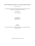
more explicit parameters (e.g., µ and ω, see figure reframpm) as well.
7
3 AIRFOIL DESIGN
Figure 1: Effect of µ on recovery shape.
If NUPA > 0, the airfoil number will be prefixed by one or two
letters with or without a space between these letters and the airfoil number, as shown in the table to the right.
If “*8” followed by two letters are given in a TRA2 or REMO
line at least two spaces after the last number, these two letters
replace “YY” in the table; “*9” followed by two letters accomplishes the same for “ZZ”.
The replacement letters precede the airfoil number if NUPA = 8
or 9, with a space if NUPA = 8 and without a space if
NUPA = 9.
NUPA
1
2
3
4
5
6
7
8
9
Letter(s)
E
S
HQ
HX
TL
MH
DO
YY
ZZ
Space
Yes
No
No
No
No
No
No
Yes
No
NUPE, NUPI, and NUPU are ignored and, therefore, columns 7–10 can be used for the airfoil identification number, if desired.
F1 specifies λ∗ , which is the beginning of the closure contribution on
the upper surface.
F2 specifies λ, which is the beginning of the main pressure-recovery
region on the upper surface.
F3 specifies RSM(us), which is the recovery specification mode for
the upper surface. It determines the interpretation of F4 and F5 as
shown in the table to the right.
¯∗; N − λ
¯ ∗ is the beginning of the closure contribution on
F6 specifies λ
the lower surface.
¯ N −λ
¯ is the beginning of the main pressure-recovery
F7 specifies λ;
region on the lower surface.
RSM(us)
0
1
2
3
RSM(ls)
0
1
2
3
F4
K
ω′
µ
µ
F9
¯
K
ω¯′
µ
¯
µ
¯
F5
µ
ω
ω
ω′
F10
µ
¯
ω
¯
ω
¯
ω¯′
F8 specifies RSM(ls), which is the recovery specification mode for the
lower surface. It determines the interpretation of F9 and F10 as shown
in the tableto the right.
¯ and µ
The values of K, µ, K,
¯ are normally rounded to three digits after the decimal point; the
∗
values of α , to two digits. F -numbers F3 and F8 allow the rounding to be changed. If the first
¯ and µ
digit after the decimal point is a, then the rounding is done to 3 + a digits for K, µ, K,
¯,
3 AIRFOIL DESIGN
8
and to 2 + a digits for α∗ . The latter is significant only if some of the α∗ values are iterated (see
below). Both F3 and F8 should specify the same value for a.
F11 specifies IT MOD, which is the iteration mode used to achieve the desired value KR of KS .
¯H.
F12 specifies KR , which is the desired value of KS = KH + K
F13 specifies Ktol , which is the tolerance on the achievement of KR ; Ktol = 0, normally.
The following iteration modes, specified by F11 , can be used to achieve the desired trailing-edge
angle as indicated by KS .
¯ H are determined
If IT MOD = 0, no iteration is performed; F12 and F13 are ignored and KH and K
by the other design parameters.
If IT MOD = 1, all αi∗ for the upper surface (i ≤ iL ) are replaced by αi∗ + ∆α∗ .
If IT MOD = 2, all αi∗ for the lower surface (i > iL ) are replaced by αi∗ + ∆α∗ .
If IT MOD = 3, all upper-surface αi∗ (i ≤ iL ) are replaced by αi∗ + ∆α∗ and all lower-surface αi∗
(i > iL ) are replaced by αi∗ − ∆α∗ .
For iteration modes 1–3, certain arcs can be excluded from the iteration by specifying a number b
after the decimal point. Thereby, b arcs from the trailing edge forward on the corresponding surface
are excluded from the iteration. For example, IT MOD = 2.7 excludes the seven arcs on the lower
surface forward of the trailing edge from the iteration.
If IT MOD = 4, K is replaced by K + ∆K.
¯ is replaced by K + ∆K.
If IT MOD = 5, K
¯ is replaced by K
¯ + ∆K.
If IT MOD = 6, K is replaced by K + ∆K and K
¯ have opposite signs, for example, if both values are
This option should not be used if K and K
determined by RSM = 2 and µ and µ
¯ have opposite signs. In this case, the effects of ∆K on Ks
are opposite for the upper and lower surfaces and the iteration may diverge or, at least, produce
unintended results.
If IT MOD = 7, αi∗L is replaced by αi∗L + ∆α∗ .
If IT MOD = 8, αi∗L +1 is replaced by αi∗L +1 + ∆α∗ .
If IT MOD = 9, αi∗L is replaced by αi∗L + ∆α∗ and αi∗L +1 is replaced by αi∗L +1 − ∆α∗ .
¯ H = KS = KR , as specified by
In all iteration modes, ∆α∗ or ∆K is determined such that KH + K
F12 . During the iteration, ∆α∗ is rounded to 2 + a digits and K to 3 + a digits to the right of the
decimal point. Therefore, KS may not be exactly equal to KR .
The TRA2 line initiates the design of the specified airfoil. The x/c and y/c airfoil coordinates,
the inner normal angles, and the velocity function v/ cos(ϕ/2 − αi∗ ) are stored in blank COMMON
arrays X, Y, ARG, and VF, respectively.
Normally, the code produces two tables containing all the νi values, including νiL , and their corresponding αi∗ values, as well as the pressure-recovery and closure-contribution parameters, in the
first line for the upper surface and in the last line for the lower surface. The first table contains
the input values; the second, the values from the final iteration. Between these two tables, one line
per iteration is written containing the values of KS and ∆α∗ or ∆K for that iteration. Other print
modes are specified by mpr in the ABSZ line (Chap. 3.4).
For example, the TRA2 line for airfoil 1098 is
TRA2
1098 4 14.5 2 1 0.65 4 14.5 2 1 0.65 6 .4 0 0
9
3 AIRFOIL DESIGN
The listing produced by this TRA2 line and the previous TRA1 line (see Chap. 3.1), assuming the
default print mode (i.e., mpr = 1, see “ABSZ Line”, Chap. 3.4), is given below. The values of K
¯ are changed by the iteration. The final values, listed in the second table, are underlined twice.
and K
¯ are underlined once. (The underlining has
The other values influenced by the changes in K and K
been added for clarity and is not produced by the code.)
EPPLER-CODE PROFIL98 V. 16.6.98
RUN
17.6.98
10:28
TRANSCENDENTAL EQUATION RESULTS AIRFOIL 1098
ITERATION 0 MODE 6
NU
ALPHA* OMEGAP OMEGA
K
MU
K H
LAMBDA LAMBDA*
23.8000 8.00
1.137 0.650 0.598 1.000 0.583060 14.50
4.00
27.8000 10.00
32.0050 12.00
60.0000 2.00
1.137 0.650 0.598 1.000 0.066661 14.50
4.00
ITERATION 1
ITERATION 2
ITERATION 3
KS= -0.360403
KS= 0.392433
KS= 0.402662
DELTA= -0.07527818
DELTA= -0.00075381
DELTA= 0.00026028
ROUNDED -0.075000
ROUNDED -0.001000
ROUNDED 0.000000
TRANSCENDENTAL EQUATION RESULTS AIRFOIL 1098
ITERATION 3 MODE 6
NU
ALPHA* OMEGAP OMEGA
K
MU
K H
LAMBDA LAMBDA*
23.8000 8.00
1.182 0.641 0.622 1.000 0.459530 14.50
4.00
27.8000 10.00
----- ----- =====
32.0050 12.00
60.0000 2.00
1.182 0.641 0.622 1.000 -0.056868 14.50
4.00
----- ----- =====
THICKNESS 18.84%, CM0=-0.1232, ALFA0= 4.8721 DEG., ETA= 1.1364
Airfoils having sharp or thin leading edges are usually not defined precisely enough in that region by
the number of points specified in the TRA1 line, even if the maximum number is specified.
Moreover, another problem arises, even if the airfoil shape is well defined. The point on the airfoil
that corresponds to the aerodynamic leading edge, νiL , usually does not coincide with one of the
computed airfoil points. Thus, for high or low lift coefficients, the leading-edge suction peak occurs
at a location that is not an airfoil coordinate. Because the velocities for all the plots and the
boundary-layer computations are computed only at the airfoil coordinates, the resulting suction peak
is, therefore, usually lower than it should be and the boundary-layer development is computed with
a shallower adverse pressure gradient near the leading edge. The low-drag range is then predicted
to be slightly too wide. This small error is unconservative and compounds an error in the same
direction arising from the integral method used for the boundary-layer computation.
Accordingly, additional points are automatically inserted near the leading edge; the code determines
how many additional points are required; the sharper the leading edge, the more points added. The
points are added in the circle plane at
νiL + ∆νj
where
∆νj = −0.5, −0.25, 0, 0.25.0.5
Finally, the values
∆νj = ±0.125,
±0.0625, ...
are used according to the amount of camber near the leading edge. No more than 13 points are
inserted, which is adequate even for very sharp leading edges.
It should be remembered that the airfoil points are normally computed for integer values of ν,
3 AIRFOIL DESIGN
10
whereas νiL is computed during the design procedure and not known in advance. The additional
points are thus located relative to the unknown leading edge. If an additional point falls too close
to an integer one, the integer one is omitted. The value ∆νj = 0 corresponds to the airfoil point
to be computed for νiL . This is the leading edge in an aerodynamic sense. At that point, the airfoil
has its maximum camber and its maximum suction peak. This point does not necessarily, however,
coincide with the geometric leading edge (i.e., x/c = 0).
As a consequence of the additional points, all airfoils are defined by more points than specified in
the TRA1 line. This is of no concern unless the airfoil is analyzed using the panel method. For
example, FLAP lines may cause the number of points to increase before the panel method is called.
Because the total number of points is restricted to 129, no more than 108 points should be specified
in the design mode. Due to the precise definition of the leading-edge region, 60 points normally
yield very precise shapes.
The code works internally with many more points in the most critical step of the conformal mapping.
This is transparent to the user. The results may, however, differ slightly from those of older code
versions, mainly for airfoils with very sharp leading edges.
Those lines in previous data sets that specify additional points near the leading edge (e.g., TRA1
lines with F1 > 998) need not to be deleted; they are now simply ignored.
Figure 2 shows the leading edge of a very thin airfoil with N = 60 in the TRA1 line with and without
additional points near the leading edge. (Note that the shape without additional points cannot be
generated using the current version of the code.) The computed airfoil points are identified on both
airfoils by tic marks perpendicular to the airfoil surface (see “STRK Line”, Chap. 5.2).
Figure 2: Thin airfoil with and without additional points near leading edge.
3 AIRFOIL DESIGN
3.3
11
RAMP Line
The RAMP line allows transition ramps to be designed without specifying several arcs with different
αi∗ forward of the pressure recovery. Instead, the length of the pressure-recovery function as specified
by λ in the TRA2 line is extended forward by ∆νf . The recovery function between the trailing edge
and λ − ∆νr , which is the aft end of the ramp, is not altered. The shape of the ramp is determined
by ∆νr and ∆νf . Over the length of the ramp, which extends from λ+∆νf to λ−∆νr , the recovery
function is replaced by a parabola with an inclined axis of symmetry. The parabola smooths the
corner that would otherwise occur at the beginning of the recovery function.
Several examples of transition ramps are given in figure 3, where the broken line is the recovery
function from the TRA2 line without a ramp and the solid line, with a ramp. The ramp is specified
by ∆νf and ∆νr only. These parameters are angles on the circle in the conformal mapping. It
should be remembered that the length in x/c between equiangular points is smaller near the leading
and trailing edges and larger near midchord.
Figure 3 illustrates the ease with which the shape of the ramp can be controlled. For example,
on the upper surface of aircraft wings, the maximum curvature should usually occur toward the
aft end of the ramp because boundary-layer transition occurs there at lower lift coefficients and
higher Reynolds numbers. The opposite is true for the lower surface. Controlling the curvature is
accomplished by changing ∆νr and/or ∆νf . Decreasing ∆νr increases the curvature of the ramp
at its aft end and vice versa; increasing ∆νf has the same effect. The first four plots illustrate
this effect for a recovery function with µ = 1, which is only slightly concave. The last four plots
show the same effect for a recovery function with µ = 0.25, which is very concave and initially very
steep. Clearly, the shape of the recovery function must be considered when designing the ramp.
For concave recovery functions, if ∆νf is too small, the intersection of the tangent to the recovery
function and the horizontal line w = 1 lies forward of the beginning of the ramp. In this case, the
code writes a message and ignores the ramp design. In such cases, either ∆νf must be increased
or ∆νr must be decreased. The length of the ramp is constrained only by the length of the given
airfoil surface.
It is permitted to change α∗ within the ramp, as can also be done within the recovery function. It is
recommended, however, that only one α∗ be specified for both the recovery function and the ramp.
NUPA, NUPE, NUPI, and NUPU are ignored;
F1 = ∆νf for the upper surface;
F2 = ∆νr for the upper surface;
F3 = ∆νf for the lower surface; and
F4 = ∆νr for the lower surface.
The RAMP line is valid for the current airfoil design only and must be inserted ahead of the TRA2
line. At the end of Subroutine TRAPRO, which computes the airfoil coordinates, the values of ∆νr
and ∆νf are reset to the default values (i.e., zero), which specify no ramp. The option of specifying
Ω′ instead of α∗ in the TRA1 line (Chap. 3.1) is independent of the RAMP line.
12
3 AIRFOIL DESIGN
Figure 3: Effect of input variation on ramps.
13
3 AIRFOIL DESIGN
The following input yields the airfoil shown in figure 4.
TRA1
RAMP
TRA2
ALFA
DIAG
77 0
4
77 4
2 5
10 60 5
2 3 3
14.5 2 -1 .7 4 12.5 2 1 .7 6 .3 0
10
-1 .08 1 2 .1 1 2 -.2 1
Figure 4: Airfoil with ramps on upper and lower surfaces.
3.4
ABSZ Line
Four values can be changed by the ABSZ line: the print mode mpr for the design iteration, the
number of lines per page in the listing, the number of points NQ in the design method, and a
precision ǫ in the panel method.
If NUPA 6= 0, mpr = NUPE, where
mpr = 0 suppresses the listing from the solution of the transcendental equation,
mpr = 1 produces the (default) listing as described in the preceding section, and
mpr > 2 produces a listing for every iteration.
NUPI and NUPU are ignored.
If F1 6= 0, the number of lines per page NP G = F1 ; the default value is 68.
If F2 6= 0, ABF A = F2 ; the default value is 1.
If F3 6= 0, EP SP A = 0.001F3 ; the default value is 0.0001.
¯ λ∗ , and λ
¯ ∗ in
The variable ABF A is a factor by which all νi values in the TRA1 lines as well as λ, λ,
the TRA2 line and ∆νf and ∆νr in the RAMP line are multiplied. This factor allows the number of
points N to be changed for a given airfoil design for which TRA1, TRA2, and RAMP lines already
exist. If the final arc limit in the TRA1 line is N, then N × ABF A must still be divisible by 4.
14
4 POTENTIAL-FLOW AIRFOIL ANALYSIS
Thus, the usual number of points N = 60, specified in the TRA1 line, can be changed to N = 108,
for example, by setting ABF A to 1.8. Note that, if the arc limits in the TRA1 lines were selected
such that they fall midway between the points on the airfoil, this will no longer be true if ABF A 6=
1. The value of ABF A must not be so large that the total number of points exceeds 120.
EP SP A specifies ǫ in the panel method, where the subpanelling is a function of ǫ. As ǫ decreases,
more subpanels are used when the induced velocity is computed at a point located very close to the
panel.
All four values, mpr, NP G, ABF A, and ǫ, remain in effect until the next ABSZ line is read. Thus,
a new ABSZ line with F2 = 1 resets ABF A to its default value.
4
Potential-Flow Airfoil Analysis
The potential-flow analysis method requires only a set of airfoil coordinates, which can come from
the design method or from the input. Because airfoil coordinates do not conveniently fit into the
format used for all the other input lines, they are read by a separate subroutine FIXLES, which is
called when an FXPR line is read. This subroutine reads or generates the coordinates and writes
them into blank COMMON arrays X(121) and Y(121) in the appropriate sequence (i.e., from the
trailing edge forward along the upper surface, around the leading edge, and back along the lower
surface to the trailing edge). The number of points NQ ≤ 121 is stored in the blank COMMON
variable NQ.
Once the coordinates are available, the slope of the upper surface δus near the trailing edge is written
into variable DLT in COMMON/PRAL/; the lower-surface slope δls , into DLTU. These slopes are
defined such that, for symmetric airfoils, δls = δus . Because many airfoils are not very smooth in
the region surrounding the trailing edge, a point (xi , yi ) on the upper surface and a point (xj , yj )
on the lower surface are selected such that xi /c ≈ 0.9 and xj /c ≈ 0.9. Then
δus = yi /(c − xi )
and
δls = −yj /(c − xj )
are set. These values are used when the lift and pitching-moment coefficients are corrected for
boundary-layer separation effects.
Once all these values have been provided by Subroutine FIXLES, the panel method is invoked. Arrays
X(121) and Y(121) are not changed. The resulting vorticities, which, in the present notation are
identical to the velocities, for α = 0◦ and α = 90◦ are stored in arrays VF(121) and ARG(121),
respectively. Thus, all the data are available to function VPR, which computes the velocity at every
airfoil point for every angle of attack.
4.1
FXPR Line
The FXPR line specifies the print mode mpa for the results of Subroutine PANEL, how the airfoil
coordinates are provided from the subsequent lines, and an option for inserting additional points
along a spline fit of the original airfoil points.
If NUPA = 0, the print mode mpa remains unchanged; the default value is 1.
If NUPA 6= 0, mpa = NUPE, where
mpa = 0 suppresses the listing,
4 POTENTIAL-FLOW AIRFOIL ANALYSIS
15
mpa = 1 or 2 lists only the headline containing the lift coefficients for 0◦ and 90◦ angle of
attack and the zero-lift angle, and
mpa ≥ 3 lists the headline plus the coordinates, the vorticities for 0◦ and 90◦ angle of attack,
and the surface slopes.
NUPI controls a coordinate transformation after which the leading edge is at x = 0, y = 0 and the
tangent at this point is vertical. The trailing edge (i.e., the midpoint between the two trailing-edge
points) is transformed into x/c = 1, y = 0. The transformation generates a new leading-edge point
for all nonsymmetrical NACA and Wortmann airfoils, which increases the number of points NQ by
1.
If NUPI = 0, no transformation is performed.
If NUPI 6= 0, the transformation is performed after the coordinates are read and possibly smoothed.
NUPU = N + 10S, (N, S ≤ 9) IF S > 0, the coordinates are smoothed.
The value N controls the derivation of the airfoil coordinates from the subsequent line or lines.
A summary of the options follows; the details are given in Chapter 4.1.3.
If N = 0 or 1, the ordinates (i.e., y/c) of a Wortmann airfoil are read; the abscissas (i.e., x/c)
are computed.
If N = 2, arbitrary coordinates xi /c and yi/c are read.
If N = 3, the upper-surface coordinates of a symmetric NACA 6-series airfoil (i.e., thickness
distribution) are read; the mean line and the coordinates of a cambered NACA 6-series airfoil
are then computed.
If N = 4, the coordinates of an NACA 4-digit-series airfoil are computed.
If N = 5, the coordinates of an NACA 5-digit-series airfoil are computed.
If N = 7, a curve of the form
ym = ax(c − x)2 + bx2 (c − x)
is computed and the x-axis of a previously given airfoil is transformed into this curve, which
yields additional camber.
If N = 8, the x-axis of a previously given airfoil is transformed into a circular arc.
If N = 9, the coordinates of a symmetric EXTRA airfoil, consisting of an ellipse and two
straight lines, are computed.
The F -numbers Fi specify additional points to be splined in (see Chap. 4.1.2).
4.1.1
Coordinate Smoothing
The second digit S of NUPU in an FXPR line allows the coordinates, read from the subsequent
lines, to be modified to eliminate irregularities. Wortmann and some other older airfoils require such
smoothing. Two options are available. If S ≥ 1 and N = 1, a mild smoothing is performed S
times; S = 3 is sufficient for most airfoils. This option applies only to Wortmann airfoils. If S 6= 0
and N 6= 1, a different smoothing, based on a compensation spline, is performed once. (Wortmann
airfoils can be smoothed using this routine if N = 0.) Both smoothing routines modify the airfoils
as little as possible. The second routine initiates a coordinate transformation exactly as NUPI 6= 0
4 POTENTIAL-FLOW AIRFOIL ANALYSIS
16
does. The first routine may result in a point x = 0, y 6= 0, even though all Wortmann airfoils already
have a point at x = 0, y = 0. An example is given at the end of Chapter 5.6.
4.1.2
Insertion of Additional Points
The F -numbers in the FXPR line (and in the PAN and FLAP lines) specify additional points to be
splined in between the original coordinates as read or generated following the FXPR line.
The F -numbers Fi are interpreted as sab.c, where s is an optional minus sign and a, b, and c may
contain more than 1 digit each. (See example below.)
If ab = 0, one point is inserted at x/c = 0.c on the upper surface or on the lower surface, if
s is a minus sign.
If ab 6= 0, c contains only one digit. The number b contains two digits if c = 4 or 5 and only
one digit otherwise. Then b new points are inserted between points a and a + 1. If s is a
minus sign, b new points are inserted between points NQ − a and NQ − a + 1, which specify
the locations of the new points relative to the trailing edge. This is helpful if NQ has been
changed since the design or coordinate input, for example, by the addition of points near the
leading edge or a transformation of the coordinates. The new points are spaced equidistantly
along the straight line between the two original points if c ≥ 5. Otherwise, the points are
spaced such that, in
x/c = (1 + cos ϕ)/2
the differences between the angles ϕ corresponding to the new points are equal (i.e., equiangular spacing).
In previous data sets, no more than nine points could be splined in between two original points and
usually c = 00 was used for equiangular spacing and c = 99, for equidistant spacing. Such data sets
are still processed correctly.
The insertion of additional points frequently improves the accuracy of the results if portions of the
airfoil have sparsely distributed points. Near the trailing edge, where the velocity changes rapidly,
the new points should be spaced equiangularly.
This option must be exercised carefully, however. The indices of all the points in arrays X and Y
falling after the inserted points are increased by the number of inserted points. The simplest way to
avoid confusion is to specify the F -numbers with decreasing values of a. Thus, a in F1 should be
greater than a in F2 , which should be greater than a in F3 , and so on. The same is true if negative
Fi are used for the lower surface.
For example, the NACA 6-series airfoils are defined by 26 points on each surface, which results in a
total of 51 points, with the leading edge at point 26. (One of the two identical leading-edge points
is omitted.) The points near the trailing edge (i.e., x1 /c = 1.00, x2 /c ≈ 0.95, and x3 /c ≈ 0.90) as
well as those near the leading edge are too widely spaced to obtain accurate results from the panel
method.
FXPR
3 502 491 261.9 251.9 21 12
FXPR
3 -251.9 -21 -12 251.9 21 12
FXPR
3 -2501.5 -201.4 -102.4 2501.5 201.4 102.4
All three lines have the same effect. The second and third lines use the option of negative Fi . The
third line uses two columns for b (i.e., two digits), which is not necessary in this example. The last
4 POTENTIAL-FLOW AIRFOIL ANALYSIS
17
two lines also function correctly if a new point was inserted at the leading edge using NUPI 6= 0;
the first line would have to be changed in this case.
In this example, two points are inserted on each surface between x/c = 0.95 and 1.00 in the equiangular spacing mode; one point, on each surface between x/c = 0.90 and 0.95 in the equiangular
spacing mode; and one point, between the leading edge and the first point on each surface in the
equidistant spacing mode. Thus, a total of eight points is inserted.
Another example is given in the next section under the specification of Wortmann airfoils.
4.1.3
Input of Coordinates
Subroutine FIXLES delivers the coordinates of an airfoil to be analyzed. In the FXPR line, NUPU
specifies the option. The line after the FXPR line is always required. It contains the airfoil name
(up to 12 characters) followed by two spaces and then one DLFF sentence containing NQ, A, R,
and T . The airfoil name is always read and written in the listing; the numbers NQ, A, R, and T
are not always used. If one of the DLFF words is specified, all preceding words must be given, even
if they are not used. The words following the last, specified word may be omitted.
If NUPU ≥ 4, the FXPR line and the succeeding line contain everything necessary to compute the
corresponding coordinates. If NUPU ≤ 3, additional information, specified in subsequent lines, is
required.
Wortmann Airfoils
If NUPU = 0 or 1 (optionally, + 10S, where S < 10), Wortmann (FX) airfoils are specified. NQ,
R, and T are ignored; A specifies a modification factor T HF .
Only the ordinates (i.e., y/c) must be given in the succeeding lines, beginning at the trailing edge
as presented in reference [7]. The abscissas (i.e., x/c) are computed in Subroutine FIXLES. The
various formats of the succeeding lines containing the ordinates are described in the Chapter 4.1.4.
In reference [7], two sizes of coordinate sets are presented: one with 49 points on each surface,
the other with 44. In the latter case, several points near the trailing edge have been omitted.
Accordingly, the code counts the number of input points and then computes the corresponding x/c
values. In the former case, the airfoil is defined by 97 points; in the latter, by 87. (The leading-edge
point is included on both surfaces in reference [7], whereas only one point is required in the code.)
In the latter case, which has only 44 input points, the spacing of the points is not very suitable for
the panel method. It is recommended that the points omitted in reference [7] be splined back in.
This is accomplished by the following FXPR line. (See Chap. 4.1.2.)
FXPR
FXPR
1 851 841 831 821 811 61 51 41 31 21
1 -61 -51 -41 -31 -21 61 51 41 31 21
Both lines insert the same points.
There is one more option available for Wortmann airfoils. Although not recommended, the thickness
and the camber of Wortmann airfoils can be modified. To accomplish this, A is used as a factor
T HF .
If T HF > 0, the thickness distribution is multiplied by T HF without changing the mean line.
If T HF < 0, all y/c values are multiplied by −T HF . Thus, the y/c values of the mean line
are also modified.
4 POTENTIAL-FLOW AIRFOIL ANALYSIS
18
For example,
FXPR
31
FX 63-126 0 -.9235
These two lines invoke the first smoothing routine (see Chap. 4.1.1) and multiply all the y/c values
by 0.9235.
Input of x/c and y/c for All Points
If NUPU = 2, the x/c and y/c values for all points must be specified.
NQ is ignored. (The number of points is determined from the input coordinates.)
If A 6= 0, all the x/c and y/c values are divided by the larger of X(1) and X(NQ) (i.e., the
more aft trailing-edge point). This normalization of the coordinates is not necessary if the x
and y values are already in the form x/c and y/c, where c is the chord.
R and T are ignored.
This is the most general coordinate-reading option. A total of NQ points are defined, each one by
xi and yi . The points can be specified in two different sequences. Both trailing-edge points, even if
identical, must be given. If they are not identical, the panel method will invoke a wake model. The
details of the sequences and the format of the coordinate lines are described in Chapter 4.1.4.
NACA 6-Series Airfoils
If NUPU = 3, an NACA 6-series airfoil (ref. [8]) is specified.
Only the thickness distribution is given; the mean line and its slope are computed.
NQ is ignored. (The number of points is determined from the input coordinates.)
A, R, and T specify the NACA 6-series mean line and a thickness ratio, where
A = a, which is the extent of the constant vorticity along the mean line (i.e., the point where
the vorticity begins to linearly decrease).
R = cℓi , which is the design lift coefficient, which determines the amount of camber.
T = thickness factor; normally, T = 1.
The succeeding lines contain the coordinates of the upper surface of a symmetrical NACA 6-series
airfoil, from the leading edge to the trailing edge, as presented in reference [8]. The number of
airfoil points NQ depends on the number of points for the symmetrical airfoil, which is determined
from the input. The format of the succeeding coordinate lines is described in Chapter 4.1.4.
It should be noted that the spacing of the points, as given in reference [8], is not very suitable for
the panel method. The option for splining in additional points should be exercised, not only near
the trailing edge but also near the leading edge. An appropriate example is given in Chapter 4.1.2.
NACA 4-Digit-Series Airfoils
If NUPU = 4, an NACA 4-digit-series airfoil (ref. [9]) is specified.
The airfoil name (e.g., NACA 4415) is given in columns 1–9, followed by two spaces, and then the
total number of points NQ to be computed.
A, R, and T are ignored.
19
4 POTENTIAL-FLOW AIRFOIL ANALYSIS
No other lines are required. The necessary airfoil parameters (see ref. [9]) are derived from the airfoil
number given in columns 6–9.
NACA 5-Digit-Series Airfoils
If NUPU = 5, an NACA 5-digit-series airfoil (ref. [10]) is specified.
The airfoil name (e.g., NACA 23012) is given in columns 1–10, followed by two spaces, and then
the total number of points NQ to be computed.
A, R, and T are ignored.
No other lines are required. The necessary airfoil parameters (see ref. [10]) are derived from the
airfoil number given in columns 6–10.
The NACA 5-digit-series airfoils having reflexed mean lines (i.e., the third digit is 1) cannot be
generated. For these airfoils, the general coordinate-reading option (i.e., NUPU = 2) must be used.
It should be noted that the coordinates presented in references [8] and [10] for the NACA 5-digitseries airfoils contain minor inaccuracies and, therefore, small discrepancies between the previously
published coordinates and those generated by the code are possible.
Transformation Using Third-Degree Polynomial Line
If NUPU = 7, the x-axis of a given airfoil is transformed into a third-degree polynomial curve of the
form
ym = ax(c − x)2 + bx2 (c − x)
The boundary conditions are
ym (0) = ym (c) = 0
′
ym
(0) = A
′
ym
(c) = −R,
where c = chord, and T is ignored.
The original airfoil must have been specified before the FXPR line with NUPU = 7 is read. Nonsymmetrical airfoils can also be modified using this option. Each point xn , yn of the original airfoil
is modified as follows. First, the point ym (xn ) on the mean line ym (x) is computed. Then, the new
point is located perpendicular to the tangent of the curve ym (x) at xn . The distance to ym (x) is
yn .
Transformation Using Circular Arc
If NUPU = 8, the x-axis of a given airfoil is transformed into a circular arc. The only diffenence
between this option and the preceding one is that the new curve ym (x) is now a circular arc through
x = 0 and x = c, with a slope at x = 0 of A degrees. This option is normally only used for cascades.
EXTRA Airfoils
If NUPU = 9, a symmetrical EXTRA airfoil is specified.
These symmetric airfoils for aerobatic aircraft are defined by an ellipse and two straight lines.
NQ is the total number of points to be computed.
A = a/c, which is the length of the half axis of the ellipse, in percent chord. (This is also the
x value of the maximum thickness.)
R = h/c, which is the thickness of the trailing edge, in percent chord.
T = t/c, which is the airfoil thickness, in percent chord.
20
4 POTENTIAL-FLOW AIRFOIL ANALYSIS
A typical EXTRA airfoil with its input are given in Fig. 5
FXPR
9
EXTRA 12 61 20 .5 12
Figure 5: EXTRA airfoil having 12-percent-chord thickness at x/c = 0.2.
4.1.4
Coordinate Lines
Only the options specified by NUPU = 0–3 require succeeding lines containing coordinates. Wortmann airfoils (i.e., NUPU = 0 or 1) are specified by pairs of ordinates (y/c)us and (y/c)ls for which
x/c values are computed by the code. The airfoils defined by arbitrary coordinates (i.e., NUPU = 2)
are specified by one pair of coordinates xn and yn for each point. The thickness distributions of
NACA 6-series airfoils (i.e., NUPU = 3) are specified in the same way. Thus, pairs of numbers are
specified in the input lines, which are read in the same way for all four options.
The coordinate lines contain one pair of numbers per line. The numbers must be separated by at
least one space. The format of the first coordinate line is used to read all the succeeding coordinate
lines.
The various options require different pairs as follows. If NUPU = 0 or 1 (i.e., Wortmann airfoils),
each pair contains the ordinate y/c of the upper surface and the ordinate of the lower surface for one
abscissa x/c. The pairs start at the trailing edge, as presented in reference [7]. The total number
of points NQ is determined from the input. If NUPU = 2, the pairs can be input in two different
sequences: the normal sequence used in the code (i.e., from the trailing edge forward along the
upper surface, around the leading edge, and then back along the lower surface to the trailing edge)
or from the leading edge to the trailing edge on the upper surface and then from the leading edge
to the trailing edge on the lower surface. The code reorders the latter into the normal sequence.
If NUPU = 3, the pairs start at the leading edge, as presented in reference [8].
4.2
PAN Line
The PAN line switches from the design to the analysis mode and, therefore, is required if the panel
method is to be employed following a design (i.e., TRA1 and TRA2 lines). The PAN line contains
the same options for the print mode and the insertion of points as does the FXPR line. A cascade
can also be defined in a PAN line.
4.2.1
Switching from Design to Analysis Mode
If 0 NUPA = 0–8, NUPE and NUPA together control the print modes (see “FXPR Line”, Chap.4.1).
NUPI controls the coordinate transformation (see“FXPR Line”, Chap. 4.1).
NUPU is ignored.
The Fi specify the additional points to be splined in (see“FXPR Line”, Chap. 4.1).
4 POTENTIAL-FLOW AIRFOIL ANALYSIS
4.2.2
21
Cascades
If NUPA = 9, the parameters of a cascade (fig. 6) are specified by F1 –F4 , where
F1 = ∆x/c;
F2 = ∆y/c;
F3 = nc , which is the number of cascade members; and
F4 = c, which is the chord in mm.
If F4 6= 0, a diagram (e.g., fig. 6) is produced in which the current airfoil is plotted twice with the
chord specified by F4 . The horizontal and vertical distances between the two airfoils are ∆x/c and
∆y/c, respectively.
The distance between the cascade members is defined by ∆x/c and ∆y/c, as shown in figure 6. A
Figure 6: Cascade parameters.
finite number of cascade members must be specified by F3 . A PAN line with NUPA = 9 merely
stores the cascade parameters and does not invoke the panel method, which must be done by another
PAN line with NUPA < 9.
The computation of cascades is a generalization of the panel method. When an individual airfoil
is analyzed, vorticity distributions are placed along the surface of the airfoil. The distributions are
determined such that the flow conditions on the airfoil surface are satisfied. When a cascade of
airfoils is analyzed, the vorticity distributions must be placed on all members of the cascade and the
amount of vorticity is again determined from the flow conditions on the surface of each member. A
cascade is usually assumed to have an infinite number of members, in which case, the flow conditions
are satisfied on all members if they are satisfied on one member.
For infinite cascades, a higher-order panel method cannot be developed with closed formulas. This is
only possible with simple low-order panel methods. To maintain higher-order precision, the cascade
members are treated exactly by the higher-order method used for the single airfoil. If the cascade
has narrow gaps between the members, the higher-order method is necessary to provide adequate
precision. Because it is not possible to have an infinite number of members and a higher-order
panel method, the number of members must be specified. If the number of cascade members nc
is 15, a good approximation to an infinite cascade results. An odd number of cascade members is
recommended because the airfoil under consideration is then in the middle of the cascade.
The convergence of the method can be checked by comparing two solutions for the cascade having
the same airfoil but different numbers of members. The most sensitive result is the second value of
cℓ in the listing from Subroutine PANEL. This cℓ value, for α = 90◦ , is equal to the lift-curve slope
of the airfoil according to potential-flow theory.
22
5 OPTIONS FOR BOTH DESIGN AND ANALYSIS MODES
The cascade parameters remain unchanged until a new PAN line with NUPA = 9 is read.
The following input generates figure 6 as well as the velocity distributions for the SH8 airfoil at an
angle of attack of 9◦ relative to the zero-lift line shown in figure 7. The number of cascade members
nc is 15 and the distance between the members is ∆x/c = 0.5 and ∆y/c = 1.0.
REMO1
TRA1
TRA26
ALFA
DIAG
PAN 9
PAN
ALFA
DIAG
REMO1
PAN 9
ENDE
*P@RTEST @1CASCADE @1OPTION
FIGS. 6+5
8 27.5 10 29.5 11 0 12 60 4
8 4 17.5 2 -1 .7 4 17.5 2 -1 .7 6 0 0
2 4 9
1
1 .5 4 1 -.2 1 -2 .3 3 2 -.4 4
.5 .7 15
2
1 .05 1 1 -.6 2 2 .05 1 2 -.2 2
*P
.6 .5 3 90
*1C
*2C
*3C
*4C
Figure 7: Velocity distributions for SH8 airfoil alone and in a cascade having 15 members (denoted
by “c”).
5
Options for Both Design and Analysis Modes
After defining an airfoil, in either the design or analysis mode, several options are available for
additional printed and plotted output. All the options are independent of the mode (design or
analysis) in which the airfoil was defined.
5 OPTIONS FOR BOTH DESIGN AND ANALYSIS MODES
5.1
23
STRD Line
The STRD line prepares the data for plotting airfoils having various chords.
NUPA is ignored.
NUPE and NUPI together form the number nn = 10NUPE + NUPI, which is the number of the
output file containing an augmented set of coordinates (see “STRK Line”, Chap. 5.2). The default
value of nn is 0.
NUPU is the plot mode mxz for subsequent plotting initiated by STRK lines.
If NUPU 6= 0, mxz = NUPU.
If mxz > 0, the x-axis is plotted.
If mxz < 0, the x-axis is not plotted.
If NUPU = 0, mxz remains as previously set. The default value is 0.
100F1 = Y BL, where |Y BL| is the height of the diagram in mm. The sign of Y BL determines
the interpretation of F2 .
100F2 = RUA, where,
if Y BL < 0, RUA is the vertical distance in mm between the chord line of one airfoil and
that of the next; and,
if Y BL > 0, RUA is the vertical distance in mm between the upper surface of one airfoil and
the lower surface of the next.
F3 = SILAF A, which is a scale factor for the label inserted above the leading edge of each airfoil.
The label contains the name of the airfoil and the thickness. The label height is SILAF A times the
airfoil chord. The airfoil name can be specified as in other diagrams. The default value of SILAF A
is 0.008, which is suitable for chords greater than 400 mm. The value of SILAF A remains in effect
until a new value is specified. If SILAF A < 0, no label is plotted.
F4 specifies the line width. The default value is the value P ENLI, which can be specified in the
REMO line (Chap. 2.2.2). The default value of P ENLI is 0.4 mm.
5.2
STRK Line
The STRK line initiates a diagram and a listing of the airfoil coordinates generated by the preceding
TRA1 and TRA2 lines or FXPR line for various chords. An STRK line must be preceded by an
STRD line.
If NUPA 6= 0, an augmented set of coordinates for each chord is listed. Each airfoil diagram increases
nn by 1 and then opens a new file LASnn.NCC. Such files can be used for numerically-controlled
milling machines, for example. The coordinates are spaced such that the straight line from one point
to the next deviates from the spline fit through the points by less than a constant times 2−NUPA .
Thus, the number of coordinates listed increases with NUPA. The value of NUPA is not stored; it
must always be specified in the STRK line that initiates the diagram.
If NUPE 6= 0, the points resulting from the design or analysis mode are identified by symbols. The
value of NUPE specifies the symbol and is valid for only one plot. Only symbols 1–9 (see fig. 12) can
5 OPTIONS FOR BOTH DESIGN AND ANALYSIS MODES
24
be specified because NUPE has only one digit. In this case, NUPE = 9 specifies symbol 10 instead
of symbol 9. Figure 2, which shows the additional points near the leading edge, was produced using
this option with NUPE = 9.
If NUPI 6= 0, the listing is produced but the diagram is suppressed.
If NUPI = 0, both the listing and the diagram are produced.
If NUPU = 1–999, the |Fi | specify up to 22 chords ci in mm, which are used for both the listing
and the diagram (if NUPI = 0). If Fi < 0, any open diagram is terminated before the diagram
containing the airfoil having chord ci is opened. If Fi > 0, the airfoil with chord ci is plotted in
the diagram that is open to further plotting. If no diagram is open or if the open diagram does
not contain sufficient vertical space, a new diagram is opened before the airfoil with chord ci is
plotted. Any airfoil having a chord ci < 1 mm is not plotted. Thus, the diagram is terminated by
−1 mm < ci < 0.
If NUPU = 0, the chords from the preceding STRK line are used.
If NUPU = 999, the Fi are the x/c locations xle of the leading edges of the airfoils in the next
STRK line with NUPU 6= 999. Negative xle are permitted. The default value of xle is 0.
The trailing edge c + xle of the first airfoil to be plotted in a diagram determines the width of the
diagram. The width can also be set by a positive xle and c < 1 mm, in which case, the airfoil that
determines the width is not plotted. The plots that exceed the width of the diagram are merely
truncated (i.e., clipped). This applies to the leading edge, if xle < 0 is specified, and to the trailing
edge, if the chord exceeds the width of the diagram.
If the leading-edge locations are not alterred by a preceding line with NUPU = 999, the largest
chord should be given first, if all the other airfoils are to be plotted in their entirety.
If only the leading-edge region is to be plotted to a large scale, a normal width is specified for the
first airfoil. The second airfoil is specified with a very large chord. Everything aft of the leading-edge
region is thus truncated. Figure 2 was produced using this option as well.
If only the trailing-edge region is to be plotted to a large scale, the first airfoil is specified with xle ≪
0 and a chord c that corresponds to the available paper size s (i.e., c = s − xle ).
Other regions (e.g., the flap hinge) can also be plotted to a large scale. First, the width of the plot
is specified and then the airfoil with large c and xle < 0, such that the desired region falls within
the diagram.
The following example plots two different airfoils in one diagram.
TRA1 and TRA2 lines (first airfoil)
STRD
1 500 5
STRK
1 500
TRA1 and TRA2 lines (second airfoil)
STRK
1 500 -0.5
Both airfoils have a chord of 500 mm and are separated vertically by 5 mm. The chord lines of both
airfoils are plotted and the diagram is terminated by the second STRK line. If the second STRK
line had specified NUPU = 0, the chord from the preceding STRK line would have been used and
the diagram would have remained open to further plotting.
The following example produces the diagrams shown in figure 8.
5 OPTIONS FOR BOTH DESIGN AND ANALYSIS MODES
REMO1
TRA1
TRA24
STRD
STRK
STRD
STRK
TRA1
TRA24
STRK
1
1
-1
2
1
2
2
2
1
*P@1@RE@2XAMPLE
28.5 3 0 10 60 2
4 18.5 2 -1 .7 4 18.5 2
32 5 -1 .15
150 100 -.1
-62 14 .016 .15
150 140
*NSUPER X
27.5 5 0 10 60 5
4 18.5 2 -1 .7 4 18.5 2
150 140 -.1
*NSUPER
25
OF AIRFOIL PLOT
-1 .7 6 .3 0
-1 .7 6 .3 0
Y
The first diagram (fig. 8) contains only the first airfoil with two chords, 150 and 100 mm, and is
closed by the chord of −0.1 mm, which is not plotted. The vertical distance between the airfoils is
1 mm and the x-axis and the labelling of the airfoils are suppressed by NUPU = −1 and F3 = −1
in the STRD line. The line width is set to 0.15 mm by F4 in the STRD line. Only the labelling
specified in the REMO line is plotted.
The second STRD line, with NUPU = 1 and F3 = 0.016, initiates the second diagram (fig. ??),
Figure 8: Two diagrams from example for STRD and STRK lines.
which contains the x-axis and the labels. The distance between the chord lines is 14 mm. The
succeeding STRK line plots the airfoil with chords of 150 and 140 mm and leaves the diagram open
to further plotting. The name of the first airfoil is set to “SUPER X”. Then, a second airfoil is
computed and plotted with chords of 150 and 140 mm, its name is set to “SUPER Y”, and the
diagram is closed. Note that the second STRD line is valid for more than one STRK line.
5 OPTIONS FOR BOTH DESIGN AND ANALYSIS MODES
5.3
26
MACH Line
The MACH line initiates two runs of the panel method; the first one, with the original coordinates
of the airfoil, and the second√one, with a new set of coordinates in which the ordinates y/c are
multiplied by the factor β = 1 − M 2 .
Following a MACH line, all velocity and pressure computations consider the compressibility effects
according to the method of reference [11], including the listing of the velocity or pressure distributions
after an ALFA line, the plot of the velocity or pressure distributions after a DIAG line, and all
boundary-layer computations.
NUPA, NUPE, NUPI, and NUPU are ignored.
F1 = M, which is the Mach number. The default value is 0.
Contrary to several other lines (e.g., ALFA, RE , FLZW, and PLW ), the input from which remains
in effect until replaced by that from a new line of the same type, the MACH line remains in effect
only until a new airfoil is defined by TRA1 and TRA2 lines or by an FXPR line and the corresponding
coordinate lines. After either of these line sequences, the Mach number is reset to 0 and another
MACH line is required if the new airfoil is to be computed with M 6= 0.
It is not necessary to insert the MACH line immediately after the definition of an airfoil. Thus, it is
possible to evaluate the differences between the incompressible and compressible flows.
The following example (fig. 9) plots a diagram containing two velocity distributions for one airfoil:
the first is incompressible; the second, compressible, with M = 0.55. (Note that some of the labels
are not specified by the example input.) The diagram includes the sonic limit if it is near the
maximum velocity on the airfoil. The Mach number M and the value Mcℓ 2 for the last α are also
plotted. The compressibility correction is invalid if the sonic limit is exceeded.
TRA1, TRA2 lines
ALFA
2 3 8
DIAG
1
MACH
.55
ALFA
DIAG
2
Figure 9: Velocity distributions for SH9 airfoil at M = 0 and M = 0.55 (identified by “c”).
5 OPTIONS FOR BOTH DESIGN AND ANALYSIS MODES
5.4
27
FLAP Line
The FLAP line exercises four options. First, the shape of an airfoil can be altered to correspond to
that due to the deflection of a simple flap. Because the panel method does not allow sharp corners
in the airfoil surface, a transition arc between the flap and the forward portion of the airfoil must
be introduced. Such a transition arc occurs ‘naturally’ on the convex side of a real wing, but not
on the concave side, where a corner is formed. This concave corner, however, is ‘smoothed’ by a
locally separated region and, therefore, it is reasonable to introduce a transition arc there as well.
This option is initiated by NUPU = 0.
The second option allows the analysis of chord-increasing flaps. It should be noted that, while the
airfoil shape that results from this variable-geometry option may have an increased chord, it does
not contain a slot and, thus, is still a single-element as opposed to a multielement airfoil. This
option is initiated by NUPU = 1–5.
The third option, specified by NUPA 6= 0, allows the modification of single points on the airfoil.
The fourth option, specified by NUPI 6= 0, concerns only the reference point for the hinge moment.
For all options that modify the shape of an airfoil,
if NUPE ≥ 8, the modified airfoil replaces the original one. In this case, the original airfoil is
completely lost and the new (modified) one can be further modified by additional FLAP lines. In
this way, it is possible, for example, to introduce a secondary flap, such as a Flettner flap, or to
introduce a flap on an airfoil after having modified its shape using the variable-geometry option.
If another FLAP line is inserted after a FLAP line with NUPE < 8, a new modification of the
old (original) airfoil will be initiated, whereas inserting another FLAP line after a FLAP line with
NUPE ≥ 8 will cause the shape as resulting from the first FLAP line to be modified.
If NUPE = 9, the thickness of the modified airfoil relative to its chord is evaluated. The new
thickness replaces the thickness of the original airfoil. For example, the deflection of a simple flap
changes the relative thickness because the airfoil chord changes.
If NUPE = 8, the evaluation of the new thickness is not performed and the thickness remains
unchanged. This is common practice in the case of simple flaps.
The panel method is invoked automatically after a FLAP line with NUPU = 0, 4, or 5 or NUPA 6= 0.
Note that the number of points may be increased by FLAP lines. The maximum number of points
on the original airfoil must be no more than 121. The panel method can accommodate up to 129
points. The modification of an airfoil with 121 points by a FLAP line with NUPU = 0 (i.e., a simple
flap) is, therefore, possible. The variable-geometry option is also allowed to increase the number of
points up to 129. A modification that yields more than 129 points, however, causes the code to
stop.
5.4.1
Simple Flap
If NUPU = 0, the airfoil shape is modified to simulate the deflection of a simple flap.
NUPA must be zero.
F1 specifies the length of the flap in percent chord.
F2 specifies the vertical location of the flap hinge in percent chord.
Thus, the flap hinge point is located at xh /c = 1 − 0.01F1 and yh /c = 0.01F2 .
5 OPTIONS FOR BOTH DESIGN AND ANALYSIS MODES
28
F3 specifies one half the transition arc length sT /c in percent chord for the upper surface. Typically,
sT /c = 0.04–0.06, depending on the amount of flap deflection.
F4 specifies the flap deflection δf in degrees, positive downward.
F5 specifies one half the transition arc length sT /c in percent chord for the lower surface. If F5 = 0
or blank, the transition arc length for the upper surface is also used for the lower surface.
For example,
FLAP
25 2 3 10
which specifies a simple, 25-percent-chord flap with a downward deflection of 10◦ . The flap hinge
is located vertically at y/c = 0.02 and the transition arc length is sT /c = 0.06 for the upper surface
as well as for the lower surface.
5.4.2
Variable Geometry
If NUPU = 1–5, the variable-geometry option is specified.
The points are renumbered during the execution of each of the following FLAP lines.
If NUPU = 1, points are deleted. The digits of the F -numbers are denoted
Fi = (−)aaa.bb
Points aaa to aaa + bb are deleted. If bb = 00, only point aaa is deleted.
The points after point aaa are renumbered. If it is intended that aaa i always be the point number
on the original airfoil, aaa of succeeding Fi must decrease. If the minus sign is given, aaa is replaced
by NQ − aaa and the points are deleted relative to point NQ, which is the last point. This is useful
on the lower surface. All negative Fi must occur before positive ones. Only the first positive Fi may
have a greater aaa than the last negative Fi .
For example,
FLAP
1 -8.08 5 2.01
which deletes points NQ − 8 through NQ, 5, and 2 and 3.
If NUPU = 2, points are inserted on the upper surface.
F1 = 100x1 /c
F2 = 100y1/c
(F3 , F4 ) = (100x2 /c, 100y2/c) and so on.
The new points are inserted in the correct sequence between or aft of the points remaining after the
deletions resulting from the FLAP line with NUPU = 1. The sequence of the points to be inserted
is arbitrary.
For example,
FLAP
2 120 -5 110 -2
which inserts two points that extend the upper surface (x/c = 1.10, y/c = −0.02 and x/c =
1.20, y/c = −0.05).
If NUPU = 3, points are inserted on the lower surface.
For example,
5 OPTIONS FOR BOTH DESIGN AND ANALYSIS MODES
FLAP
29
3 100 -2.5 120 -5
which inserts two points that extend the lower surface (x/c = 1.00, y/c = −0.0250 and x/c =
1.2000, y/c = −0.0500).
Normally, some points must be deleted by a FLAP line with NUPU = 1 before new points are inserted.
If NUPU = 4 or 5, additional points are splined in. The F -numbers are interpreted just as they are
for the FXPR line, including the option of negative Fi .
Fi = (−)aab.dd
If NUPU = 5, in addition to the splining in of points, a transformation is performed that rotates the modified airfoil around x = 0, y = 0 and stretches it so that the first point becomes
x/c = 1, y/c = 0. The option NUPE = 9 can also be used.
Care must be exercised because deleting points (i.e., NUPU = 1) as well as inserting new points
(i.e., NUPU = 2 or 3) changes the sequence numbers of the points and the total number of points
NQ. For splining in additional points, the alterred point numbers must be taken into account. An
example is given in figure 10.
For example,
FLAP
4 -24 -16 22 13
which inserts a total of 15 points, all with equiangular spacing: four points between points NQ − 2
and NQ − 1, six points between points NQ − 1 and NQ, two points between points 2 and 3, and
three points between points 1 and 2.
The application of the four FLAP lines given in this section to an NACA 23015 airfoil, defined
originally by 61 points, is shown in figure 11. The following steps occur.
The original upper surface is maintained up to the original trailing edge, although some points near
the original trailing edge are deleted because the close spacing there is no longer necessary although
it is near the new trailing edge (x/c = 1.20, y/c = −0.05), as described below.
On the lower surface, points NQ − 8 through NQ are deleted, which includes the lower-surface,
trailing-edge point.
On the upper surface, two points are inserted at x/c = 1.10 and x/c = 1.20. Two points are
splined in between the original trailing edge and the new point at x/c = 1.10; three points, between
x/c = 1.10 and x/c = 1.20.
On the lower surface, the last point of the original airfoil that was not deleted is near x/c = 0.84.
Its number is 51, after the deletion of three points and insertion of two on the upper surface. Aft of
that point, only two points are inserted: one at x/c = 1.00 (number 52 or NQ − 1) and the other
at x/c = 1.20 (number 53 or NQ). The distances between these points as well as between the last
point on the original airfoil and the first inserted point are larger than those on the upper surface.
Therefore, four and six points, respectively, are splined in using negative Fi . This procedure does
not require knowledge of the absolute point numbers and still functions properly if, for example, the
transformation (i.e., NUPI = 1) that produces the vertical tangent at x = 0, y = 0 is performed by
the FXPR line (see Chap. 4.1). This is actually performed in this example.
30
5 OPTIONS FOR BOTH DESIGN AND ANALYSIS MODES
Original point numbers
(before deleting points by
FLAP line with NUPU = 1)
Point numbers after deleting
points by FLAP line with
NUPU = 1 and before inserting points by FLAP lines
with NUPU = 2 and 3.
Point numbers after inserting points by FLAP lines
with NUPU = 2 and 3.
Figure 10: Alteration of airfoil point numbers during exercise of
variable-geometry option.
Figure 11: NACA 23015 airfoil with and without variable-geometry modification.
5.4.3
Modification of Individual Points
If NUPA 6= 0, individual points are modified.
NUPE, NUPI, and NUPU are ignored.
F1 = ni , which is the point number, the ordinate y/c of which is changed by F2 .
F2 is the vertical component of the change perpendicular to the surface in percent chord. Positive
F2 denotes a change toward the exterior of the airfoil (i.e., a bump); negative F2 , a change toward
the interior (i.e., a dip).
(F3 , F4 ) and so on allow six more points to be modified.
For example,
31
5 OPTIONS FOR BOTH DESIGN AND ANALYSIS MODES
FLAP19
3 .01 37 -.01
which moves point number 3 toward the exterior of the airfoil by 0.01-percent chord and point
number 37 toward the interior by the same amount. The modified airfoil replaces the original one
because NUPE = 9.
5.4.4
Moment Reference Points
The ALFA line invokes Subroutine MOMENT, which computes the pitching-moment and hingemoment coefficients cm and ch , respectively, for each angle of attack. The reference point for cm is
normally the quarter-chord point and, for ch , the leading edge. The coefficients are stored so they
are available for other (e.g., boundary-layer) computations. Depending on the print mode mcm,
the coefficients can be listed immediately after they are computed. A FLAP line with NUPU = 0
automatically shifts the reference point for ch to the flap hinge point. The computation of ch is
performed such that only that portion of the airfoil aft of the reference point contributes to ch . The
hinge-moment coefficient ch is nondimensionalized by the airfoil chord, not by the flap chord. This
works properly only if the coordinates are not normalized by a FXPR or PAN line with NUPI 6= 0.
Occasionally, moments relative to other reference points must be computed, which can be accomplished by means of a FLAP line with NUPI 6= 0.
NUPA, NUPE, and NUPU are ignored.
If NUPI = 1, the reference point for both cm and ch is shifted to
x/c = 0.01F1
y/c = 0.01F2
If NUPI = 2, the reference point for both cm and ch is shifted to the point specified by F1 and F2 as
with NUPI = 1 but the calculation of cm excludes that portion of the airfoil forward of the reference
point.
If NUPI > 3, the F -numbers are ignored and the reference point for cm is the flap hinge point. The
calculation of cm is performed as with NUPI = 2.
This FLAP line immediately initiates the computation of cm and ch about the new reference point
for all α values in the currently valid ALFA line. Depending on the print mode specified in this ALFA
line, a listing of the moment coefficients is produced, in which the reference point is given.
The option NUPI = 1 is useful in two specific cases. It can be used to determine the aerodynamic
center, for which cm is constant with α and the value of ch can be used to evaluate the bending
moment of ribs in a wing.
The options NUPI > 3 are relevant only in conjunction with other FLAP lines because the values
of cm and ch would otherwise be identical. These options can be exercised, however, after a FLAP
line with NUPE = 9. Another FLAP line then allows another flap to be introduced and the moment
relative to the previous reference point (e.g., the previous flap hinge point) to be computed. The
authority of Flettner flaps or trim tabs can thus be analyzed.
The following input lines produce the listing below.
REMO1
*PLISTING CHAPTER FLAP-LINE
FXPR
4
NACA 0009
61
0
0
09
ALFA101003 -10 0 10
FLAP 1
26.148 0
ALFA
FLAP 2
40 0
ALFA
FLAP 9
ALFA101003
FLAP 3
ALFA101003
FLAP
ALFA101003
25 0 3 5
-10 0 10
-10 0 10
8 -1.49 2 10
-10 0 10
5 OPTIONS FOR BOTH DESIGN AND ANALYSIS MODES
PANEL METHOD NACA 0009 9%
CL=-0.000000486, 6.74718 ALPHA0=-0.000004127 MACH=0
Airfoil NACA 0009 9%
Moments
delta=0 deg.,Hinge at x=0 y=0
Alpha relative to the chord l.
ALPHA
CM
CH
CL
-10.00
0.013212
0.301082 -1.168387
0.00
0.000000
0.000000
0.000000
10.00 -0.013212 -0.301081
1.168386
CL(LIN)
-1.100000
0.000000
1.100000
Airfoil NACA 0009 9%
Moments
delta=0 deg.,Hinge at x=0.26148 y=0
Alpha relative to the chord l.
ALPHA
CM
CH
CL
-10.00 -0.000007
0.111141 -1.168387
0.00
0.000000
0.000000
0.000000
10.00
0.000007 -0.111141
1.168386
CL(LIN)
-1.100000
0.000000
1.100000
Airfoil NACA 0009 9%
Moments
delta=0 deg.,Hinge at x=0.4 y=0
Alpha relative to the chord l.
ALPHA
CM
CH
CL
-10.00
0.060703
0.060703 -1.168387
0.00
0.000000
0.000000
0.000000
10.00 -0.060702 -0.060702
1.168386
CL(LIN)
-1.100000
0.000000
1.100000
PANEL METHOD NACA 0009 9%
CL=0.363964, 6.742775 ALPHA0=3.089734 MACH=0
Airfoil NACA 0009 9%
Moments
delta=5 deg.,Hinge at x=0.75 y=0
Alpha relative to the chord l.
ALPHA
CM
CH
CL
-10.00
0.011974
0.000741 -0.808646
0.00 -0.049861 -0.004984
0.363829
10.00 -0.108545 -0.010336
1.524523
CL(LIN)
-0.760129
0.339871
1.439871
Airfoil NACA 0009 9%
Moments
delta=5 deg.,Hinge at x=0.75 y=0
Alpha relative to the chord l.
ALPHA
CM
CH
CL
-10.00
0.000741
0.000741 -0.808646
0.00 -0.004984 -0.004984
0.363829
10.00 -0.010336 -0.010336
1.524523
CL(LIN)
-0.760129
0.339871
1.439871
PANEL METHOD NACA 0009 9%
32
CL=0.783348, 6.719803 ALPHA0=6.649134 MACH=0
Airfoil NACA 0009 9%
Moments
delta=10 deg.,Hinge at x=0.9192 y=-0.014887
Alpha relative to the chord l.
ALPHA
CM
CH
CL
CL(LIN)
-10.00 -0.014017 -0.000858 -0.391355
-0.368595
0.00 -0.019818 -0.001147
0.781171
0.731405
10.00 -0.024346 -0.001359
1.928365
1.831405
Six blocks of results are produced. Each contains a table with α, cm , ch , cℓ , and cℓ (lin), where cℓ
is computed from the potential-flow (i.e., inviscid) velocity distribution and cℓ (lin) includes viscous
effects merely by setting the lift curve slope to 2π or 0.11 per degree.
The first block contains cm about the quarter-chord point and ch about the leading edge. Because
no portion of the airfoil is forward of the reference point for ch (i.e., the leading edge), ch is identical
5 OPTIONS FOR BOTH DESIGN AND ANALYSIS MODES
33
to the moment coefficient about the leading edge.
The second block contains cm about x/c = 0.2605, y/c = 0, which is the aerodynamic center. The
hinge-moment coefficient ch is still computed about the leading edge.
The third block contains cm and ch about x/c = 0.4, y/c = 0, which is a hinge point. The contribution of the portion of the airfoil forward of the hinge point is excluded.
The fourth block, which concerns a 25-percent-chord flap deflected 5◦ , contains cm about the previous hinge point x/c = 0.4, y/c = 0 and ch about x/c = 0.75, y/c = 0, which is the hinge point
introduced by a preceding FLAP line.
The fifth block contains cm and ch about x/c = 0.75, y/c = 0.
The sixth block, which concerns an additional 8-percent-chord flap deflected 10◦ , contains cm about
x/c = 0.75, y/c = 0 and ch about the new hinge point x/c = 0.9192, y/c = −0.0149.
5.5
ALFA Line
The ALFA line initiates:
the storage of up to 22 angles of attack specified by the F -numbers (all α values remain
available for other options),
the inviscid computation of the pitching-moment and hinge-moment coefficients for the specified angles of attack (these coefficients also remain available for other computations), and
additional listings specified by print modes mxy, mpa, and mcm.
One last option, which lists the second derivatives of the velocity or pressure distributions at various
angles of attack, is described at the end of this section.
NUPA and NUPE determine the print modes.
If NUPA = 0, mxy, mcm, and mpa remain as previously set.
If NUPA 6= 0, mxy = NUPE and mcm = NUPA.
If NUPA = 1, mxy = NUPE, mcm = NUPA, and, additionally, mpa = NUPE + 1.
If mxy 6= 0, the airfoil coordinates and the velocity, or pressure, distributions for all the
specified α (up to 14) are listed. This is called an x-y-V listing. If mxy = 0, no listing is
produced.
If mcm = 1, the pitching-moment cm and hinge-moment ch coefficients for all the specified
values α are listed. If mcm 6= 1, no listing is produced.
If mpa = 0, no listing from Subroutine PANEL is produced.
If mpa = 1 or 2, only the headline from Subroutine PANEL is listed.
If mpa > 3, the headline, the airfoil coordinates, and the vorticities for α = 0◦ and α = 90◦
from Subroutine PANEL are listed.
The default values are mxy = 1, mcm 6= 1, and mpa = 1.
5 OPTIONS FOR BOTH DESIGN AND ANALYSIS MODES
34
The print modes are summarized in the following table.
NUPA
0
1
1
1
NUPE
ignored
0
1
≥2
≥2
≥2
0
≥1
Output
x-y-V listing as before
cm and ch listing, headline from PANEL, no x-y-V listing
x-y-V listing, cm and ch listing, headline from PANEL
x-y-V listing; cm and ch listing;
headline, vorticities, and slopes from PANEL
mpa for PANEL listing remains as before, no x-y-V listing
x-y-V listing, mpa for PANEL listing remains as before
Note that the print mode mpa cannot be set to 0 in an ALFA line. This must be done in an FXPR or
PAN line. Setting mpa in the ALFA line (i.e., NUPA = 1) is only useful if the moment coefficients
are to be listed.
NUPI and NUPU specify the details of the x-y-V listing and also the corresponding plot produced
by a DIAG line.
If NUPI = 0, the α values are relative to the zero-lift line and the x-y-V listing and the DIAG plot
contain velocity distributions.
If NUPI = 1, the α values are relative to the x-axis and the x-y-V listing and the DIAG plot contain
velocity distributions.
If NUPI = 2, the α values are relative to the zero-lift line and the x-y-V listing and the DIAG plot
contain pressure (Cp ) distributions.
If NUPI = 3, the α values are relative to the x-axis and the x-y-V listing and the DIAG plot contain
pressure (Cp ) distributions.
If NUPU = 0–22, NUPU specifies nα , which is the number of F -numbers (i.e., α values) to be read.
The number of F -numbers n is determined from the input. If n > nα , nα is set to n. Thus, it is
simplest to set NUPU to 1 and let the code count the α values.
If NUPU > 22, a listing containing only the point numbers, x, y, and ν is produced and nα is set
to 0.
If NUPU = 0, NUPI, nα , and the values of αi from the preceding ALFA line with NUPU 6= 0 are
used.
The Fi , where i = 1, ..., nα , specify the angles of attack αi in degrees.
If Fi = −99.ab, αi = αk∗ , where k = ab. If k = 0 or k > nα , then k = i.
This option allows α∗ values from the airfoil design to be used as αi . (Remember that the velocity
over airfoil segment i is constant at this α.) This option is useful if the values of αi∗ have been
changed by iteration during the design procedure. If this option is specified after an airfoil analysis
or if k = i < nα , the αi is skipped.
Internally, the code uses the angle of attack relative to the zero-lift line. If NUPI = 1 or 3, all angles
of attack relative to the x-axis are converted to values relative to the zero-lift line and then back to
values relative to the x-axis for output only. If the option Fi = −99.ab is used with NUPI = 1 or
3, the αi∗ are converted to values relative to the x-axis for output.
The following examples illustrate the use of the ALFA line.
ALFA21
1 1 -99 -99.05 3
No moment coefficients are listed (mcm = NUPA = 2 6= 1), the x-y-V listing containing velocities
5 OPTIONS FOR BOTH DESIGN AND ANALYSIS MODES
35
is produced (NUPA 6= 0 and, therefore, mxy = NUPE = 1; NUPI = 0), and α1 = 1◦ , α2 = α2∗ ,
α3 = α5∗ , and α4 = 3◦ , all relative to the zero-lift line (NUPI = 0).
ALFA
3
1 2 4 6 8 10
Print modes mcm and mxy remain as previously set (NUPA = 0). If mxy 6= 0, the x-y-V listing
containing pressure coefficients is produced (NUPI > 2) with α = 2◦ , 4◦ , 6◦ , 8◦ , and 10◦ relative to
the x-axis (NUPI = 3).
ALFA
[no additional input]
NUPI, nα , and the values of αi from the preceding ALFA line with NUPU 6= 0 are used and print
modes mxy, mcm, and mpa remain as before.
ALFA20
NUPI, nα , and the values of αi from the preceding ALFA line with NUPU 6= 0 are used. The momentcoefficient listing and the x-y-V listing are not produced (NUPA = 2 6= 0; therefore, mxy = NUPE = 0).
A special option lists the second derivatives of v(φ) in the x-y-V listing. This allows the curvature
of v(φ), usually in the ramp area, to be checked. (See ref. [3].) If an αi 6= 0 and αi+1 = αi , the
second derivative of the velocity (or pressure) distribution is listed for αi+1 .
5.6
DIAG Line
The DIAG line initiates the plotting and labelling of two different diagrams: the x-y-V diagram,
which contains the airfoil shape and velocity or pressure (Cp ) distributions or a so-called pressureenvelope diagram, which is relevant for cavitation on hydrofoils.
If NUPA 6= 0, the lines in the x-y-V diagrams are plotted as polygons instead of splined curves. The
coordinate points, in this case, can be distinguished by the corners of the polygons.
If NUPE = 1, experimental data are inserted into the x-y-V diagram (see below).
NUPI determines the type of diagram to be plotted and the line type to be used (see below).
NUPU specifies the plot mode mbt, by which different sets of data can be plotted in one diagram,
V (s) near the leading edge can be plotted, and the airfoil points can be identified by symbols.
The three digits of NUPU are designated abc.
If c = 0, one set of data is plotted, axes are drawn, and the diagram is terminated (i.e., closed
to further plotting).
If c = 1, one set of data is plotted and the diagram remains open to further plotting.
If c = 2, one set of data is plotted into the open diagram, axes are drawn, and the diagram
is terminated.
If c = 3, one set of data is plotted into the open diagram, which remains open to further
plotting.
If b 6= 0, the airfoil points are identified by symbol b, as defined in figure 12. In this case, only
the first eight symbols are available; symbol 9 is a flag perpendicular to the airfoil surface.
If a 6= 0, V (s) near the leading edge is plotted. The velocities on the lower surface are plotted
as negative values.
Obviously, plot mode mbt is valid only for the one DIAG line in which it is specified.
5 OPTIONS FOR BOTH DESIGN AND ANALYSIS MODES
36
Figure 12: Available symbols and their numbers. Symbol 10 is a flag perpendicular to the local
tangent.
5.6.1
Pressure-Envelope Diagram
If NUPI = 1, a pressure-envelope diagram is plotted. The abscissa is −Cp,min and the ordinate, α.
All α values in the preceding ALFA line are used. The size of the frame depends on the α values.
If the vertical extent of the frame must be increased to accommodate a succeeding set of data, this
can be accomplished by setting F1 and F2 6= 0.
If F1 6= 0, F1 = αmin in degrees.
If F2 6= 0, F2 = αmax in degrees.
5.6.2
x-y-V Diagram
If NUPI 6= 1, the x-y-V diagram is plotted.
If NUPI = 0, the curves in the x-y-V diagram are solid.
If NUPI ≥ 2, NUPI is the line type as defined in Chap. 6.7.4.
The x-y-V diagram contains the airfoil shape and the velocity or pressure distributions for all α
values in the preceding ALFA line. The ordinate is V , if NUPI = 0 or 1 in the ALFA line or −Cp , if
NUPI = 2 or 3.
Scaling
Usually, the diagrams are produced by means of a printer, in which case, it is helpful to specify the
size of the diagrams in the input. The length of the x/c-axis in the velocity or pressure distribution
is specified by 100F1 , which is the unit length (i.e., x/c = 1) of the x/c-axis in mm. The default
value is 200 mm.
For example,
DIAG
140
which specifies a length of 140 mm for the x/c-axis.
Note that the x/c-axis can extend beyond x/c = 1 for airfoils with flaps or variable geometry. Only
DIAG lines that open a diagram (i.e., NUPU = 0 or 1) can alter the unit length.
Extension of Frame
The size of the frame for the x-y-V diagram is determined from the data available when the diagram
is opened (i.e., NUPU = 0 or 1). The data to be plotted from this line, including the experimental
data, if NUPE = 1, are evaluated before the frame is opened and the frame is sized accordingly.
Without additional input, the upper edge of the frame is set to V = 2.5 or Cp = −3. The curves
37
5 OPTIONS FOR BOTH DESIGN AND ANALYSIS MODES
are not plotted beyond this limit.
The upper edge of the frame can be extended by specifying F1 in a DIAG line with NUPU = 0 or
1, in which case F2 specifies Vlimit or (Cp )limit .
The upper edge of the frame will be extended if the limit specified by F2 is greater than that derived
from the data. This can be applied in two ways as follows.
If the data corresponding to the first DIAG line (i.e., NUPU = 0 or 1) exceeds the default limit
V = 2.5 or Cp = −3 and the entire curves are to be plotted.
If, following a DIAG line with NUPU = 1, the curves from succeeding DIAG lines with NUPU = 2
or 3 require a larger frame than those from the first DIAG line.
Labelling
Without additional input, the axes are labelled “α relative to the x-axis” or “α relative to the zero-lift
line” and all α values used for the diagram are plotted in the upper, right corner. The airfoil name
and thickness in percent chord, valid for the DIAG line terminating the diagram (i.e., NUPU = 0 or
2), are plotted inside the airfoil or, if the airfoil is too thin, below it.
If NUPU = 0 and only one α value is input, this value is included in the label “α = ... relative to
the ...” and the plotting in the upper, right corner is omitted.
In all DIAG lines with NUPI = 0, additional input can begin at least three columns after the last
F -number; if no F -number is present, in column 13 or higher. One or more DLFF sentences can
be given that contain one or more groups of three numbers as follows.
±i, ±x/c, e, ±i, ±x/c, e, ...
Each group of three numbers plots the ith α value near the corresponding curve. The value is
plotted such that the corner e of the label rectangle (fig. 13) is located at x/c along the curve. If
the sign of x/c is negative, the curve corresponding to the lower surface is labelled; if positive, the
curve for the upper surface is labelled. If a minus sign precedes i, “α =” is plotted ahead of the α
value. The input e = 1 at the end of a sentence can be omitted; the next sentence must then begin
with ±i for the next group.
The label rectangle encompasses the label and a small gap. The e values corresponding to the four
corners are shown on the left side of figure 13. The right side of figure 13 shows an example in
which corner 4 is located along the curve.
If labelling information is input, the α values are not plotted in the upper, right corner.
e=1
e=4
◦
α
=
4
e=2
e=3
H
HHe = 4
HH
HH
H
α = 4◦
Figure 13: Label rectangles.
Note that the character “F” in any DLFF word can be used to continue the input in the next line.
The airfoil name to be plotted can be changed by inputing *N and the new name as a character
string at least three columns after the end of the last DLFF sentence. The name must be terminated
by two spaces. Thus, the name cannot contain two successive spaces.
5 OPTIONS FOR BOTH DESIGN AND ANALYSIS MODES
38
After *Z, a character string can be given that will be plotted after the label(s) explaining the first
α value.
After *i, where i = 1, 2, ... 9, a character string can be given that will be plotted after the label
initiated by the ith group of three numbers.
If only one α value is valid, its value is omitted in the label(s) along the curve.
If i < −30, |i| − 30 specifies the number of the α value and the cℓ value is written near the curve
instead of the α value. This is normally done in the first group. This option is useful if the Mach
number is not zero. The α label is then omitted.
If “F” is the last character of a character string, the current flap data are plotted as “cf % Flap δf◦ ”,
where cf is the flap chord and δf is the deflection. These data are not plotted if δf = 0◦ . The input
*iF or *ZF adds only the flap data to the labels.
Font @1 (see ref. [6]) is the default font for the airfoil name and, therefore, switching to capital
Latin letters is superfluous, in this case.
Experimental Data
Experimental data can be inserted into an x-y-V diagram. If NUPE = 1 in the DIAG line that opens
a diagram (i.e., NUPU = 0 or 1), the succeeding lines, which have “X”, “Y”, or “E” in the first
column, specify the experimental data as follows.
The X lines contain the x/c values.
The Y lines contain the velocities, if the preceding ALFA line has NUPI ≤ 1, or pressure
coefficients, if NUPI ≥ 2.
The E line terminates the experimental data.
The X and Y lines are read by the same subroutine as are the experimental data for the CDCL
diagram (see Chap. 6.7). Thus, the same options are available. The first line in the key is
solid with the explanation “Theory”.
The available symbols are shown in figure 12.
The following example produces the diagram shown in figure 14.
REMO1
*P
*9US
TRA1
88 0 5 60 -5
TRA29
88 4 17.5 2 -1 .6 4 17.5 2 -1 .6 3 0 0
ALFA201 2 -99.9 0
DIAG 1
1 0 2.2
1 .65 2 -2 .3 3 1 -.25 3
*2@1Plain
X 100 45 50 60 65
Y 100 135 140 135 160 2
*T@1Fictitious Experiment
E
FLAP
25 0 3 15
ALFA 1 2 3 0
DIAG
2
-1 .1 2 2 .16 3 2 -.7 2 1 -.2 F
1
*ZF *2, @1Flap
*3, @1Flap
The velocity distributions for two different flap deflections (0◦ and 15◦ ) are plotted in one diagram
by means of DIAG lines with NUPU = 1 and NUPU = 2. The labels “α =” are added when i is
negative. The labels “Plain” and “25% Flap 15◦ ” are inserted after the labels with i = 1, which
occcurs once in each DIAG line. The label “Flap” is inserted after the α labels corresponding to the
second and third groups of three numbers. Ficticious experimental data are included.
The following example produces figure 15.
5 OPTIONS FOR BOTH DESIGN AND ANALYSIS MODES
39
Figure 14: Velocity distributions for unflapped and flapped US88 airfoil.
REMO1
TRA1 1111
TRA2 1111
ALFA
1
DIAG
1
FLAP 9
ALFA 1001
DIAG
3
FLAP
ALFA 1001
DIAG
2
*P
0 5 60 -5
4 17.5 2 -1 .7 4 17.5 2 -1 .7 3 .2 0 0
0
0 1.6
25 0 3 5
0
1 .12 3
*Z@1Flap
8 -1.49 2 10
0
1 .4 2
*Z@1Double Flap
The FLAP lines of this example are the same as the last two FLAP lines in the example for listing
the moment coefficients. The velocity distributions for three shapes are plotted in one diagram by
NUPU = 1, 3, and 2. Only one α value is given. This value is included in the explanation line and
omitted from the labels near the curves. The additional text given after *Z is plotted at the location
given by the group of three numbers. Using *1 instead of *Z would have the same effect.
The third example illustrates the smoothing option for Wortmann airfoils. The velocity distributions
for the original coordinates and those after three smoothings are shown in figure 16.
5 OPTIONS FOR BOTH DESIGN AND ANALYSIS MODES
40
Figure 15: Velocity distributions for airfoil 1111, unflapped and with single and double flaps.
FXPR
FROM THE NEW BOOK
FIG. 13
FX 63-137
FX63-13701 000 000
82
40 249 169 501 373 818 630 1189 921
FX63-137 7 1601 1219 2043 1514 2516 1794 3018 2052 3553 2284 4114 2479
FX63-13713 4711 2631 5323 2729 5962 2768 6605 2745 7273 2668 7927 2530
FX63-13719 8590 2343 9204 2098 9804 181310331 147510823 111211221 716
FX63-1372511578 30711833 -10312042 -48612137 -84812191-116712128-1460
FX63-1373112024-168811792-189511522-203411122-216110704-222010165-2277
FX63-13737 9622-2263 8975-2256 8323-2180 7611-2122 6864-1978 6089-1855
FX63-13743 5304-1699 4480-1482 3625-1254 2740 -995 1820 -636 985 -317
FX63-13749 000 000
ALFA
1 4 8 12
DIAG
1
FXPR
30
FROM THE NEW BOOK
FX 63-137
FX63-13701 000 000
82
40 249 169 501 373 818 630 1189 921
FX63-137 7 1601 1219 2043 1514 2516 1794 3018 2052 3553 2284 4114 2479
FX63-13713 4711 2631 5323 2729 5962 2768 6605 2745 7273 2668 7927 2530
FX63-13719 8590 2343 9204 2098 9804 181310331 147510823 111211221 716
FX63-1372511578 30711833 -10312042 -48612137 -84812191-116712128-1460
FX63-1373112024-168811792-189511522-203411122-216110704-222010165-2277
FX63-13737 9622-2263 8975-2256 8323-2180 7611-2122 6864-1978 6089-1855
FX63-13743 5304-1699 4480-1482 3625-1254 2740 -995 1820 -636 985 -317
FX63-13749 000 000
ALFA
1 4 8 12
DIAG
2
-1 .2 1 2 .19 3 3 .4 2 2 -.16 4 3 -.25 1
5.7
PUXY Line
The PUXY line writes the airfoil coordinates x/c and y/c and the inner normal angles β to a file
having the name of the input file and the extension “PU”.
6 BOUNDARY-LAYER ANALYSIS
41
Figure 16: Velocity distributions for original and smoothed FX 63-137 airfoil.
Columns 1–5 in each output line contain the airfoil name. If this name comes from the analysis
mode, characters 3–7 of the name are used. If this name comes from the design mode, a space
followed by the four digits of the airfoil number are used. Columns 6–8 contain the number of the
first point written in that line. Columns 9–80 contain four groups of three numbers each, which are
the x/c, y/c, and β values for one point. No decimal points are written. The x/c and y/c values
in this file can be read using format F6.5 and the β values, format F6.4.
6
6.1
Boundary-Layer Analysis
Fundamentals
The computation of the boundary-layer development is performed by means of an integral method
(see ref. [3]). This method requires as input the Reynolds number R and the potential-flow velocity
distribution U(s), where s is the arc length from the stagnation point along the surface of the airfoil.
The velocity distributions are computed in either the design or the analysis mode.
The basic results of this approximate method are the momentum thickness δ2 (s) and the shape
factor H32 (s). Also the displacement thickness δ1 (s) and the shape factor H12 (s) are evaluated.
The momentum thickness is most significant for the viscous drag; the shape factor indicates the
shape of the boundary-layer profile. Increasing H32 corresponds to a more favorable pressure gradient.
All results together allow the approximate evaluation of displacement, separation, and transition of
the boundary layer, the airfoil drag, and the occurence and effect of laminar separation bubbles.
The prediction of boundary-layer separation has not been changed since 1963 (ref. [4]). Separation
42
6 BOUNDARY-LAYER ANALYSIS
is predicted when H32 decreases to 1.51509 in a laminar boundary layer and when H32 decreases to
1.46 in a turbulent boundary layer. A displacement iteration was developed in 1980 (ref. [2]).
6.1.1
Criteria for Boundary-Layer Transition
In code versions since 1980, boundary-layer transition was predicted by means of a local criterion.
In 1996, a new empirical transition criterion was implemented that considers the instability history
of the laminar boundary layer, which avoided the long computing time of the eN method while
achieving similar results, in most cases.
Since then, computing power has increased dramatically, which has negated the disadvantage of the
eN method. Moreover, the faster computers allowed a very large number of solutions of the OrrSommerfield equation to be computed and tables to be constructed from which the amplification
rates of the Tollmien-Schlicting (TS) waves can be evaluated with adequate precision by interpolation. This increases the speed of the eN method such that the boundary-layer computations require
only 10 to 30 times more time than with the empirical criterion, which is compensated by the higher
computer speed.
The laminar boundary layer is initially stable. During its development, a combination of Reynolds
number and shape factor must be found for which the first TS wave becomes unstable. This
stability limit has been evaluated for many shape factors. A table was then constructed that allows
the stability limit for a given boundary-layer development to be evaluated precisely by interpolation.
This evaluation also yields the frequency of the first unstable TS wave.
The amplification rate of a TS wave depends on the local Reynolds number and the shape factor
of the boundary-layer flow in which it develops and on its frequency. An amplification table must
therefore contain values depending on three parameters. In stability theory, these three parameters
are the Reynolds number based on the displacement thickness δ1 , the shape factor H12 , and a
nondimensional frequency β. The current amplification table contains more than 40,000 values.
The boundary-layer computation begins with the search for the first unstable TS wave with its
nondimensional frequency βcrit . This yields also the natural frequency fcrit . A frequency range
with 64 frequencies fi is defined around fcrit . For all fi , the amplifications are evaluated and their
natural logarithms are summarized into the amplifications ln ai (s). At any position s along the
airfoil surface, the maximum amplification
n(s) = max {ln ai (s)}
is evaluated by quadratic interpolation. If n reaches the specified value N, transition is assumed.
During the development of the laminar boundary layer, the frequency of the most amplified TS wave
varies considerably. Some of the TS waves that are initially amplified may be damped later whereas
others may be amplified. Sometimes, the frequency of the most amplified TS wave is outside the
defined frequency range. The boundary-layer computation is then halted and restarted at the first
instability using an expanded frequency range. Two typical examples of amplifications for many
frequencies are shown in figure 17. The amplifications are plotted using dashed lines where the
length of the dash is proportional to the frequency. Thus, higher frequencies are represented by
shorter dashes and lower frequencies, by longer dashes. This gives a qualitative impression of the
length of the TS waves. The ordinate is the airfoil point number. The amplifications are plotted
only for these points although they are usually computed at many intermediate points as well.
The examples in figure 17 show that higher frequencies are often damped out after initially being
amplified, whereas lower frequencies are amplified later and finally reach the transition value.
6 BOUNDARY-LAYER ANALYSIS
43
Figure 17: Examples of amplification diagrams.
This method seems straightforward, although the value of N must be determined empirically. The
amplification is only a factor by which very small initial disturbancies are amplified. The amplitude
of the TS waves at the beginning of the transition process has been extensively investigated. Measurements in low-turbulence wind tunnels correspond to an N of 11 to 13. Measurements in flight
correspond to N values up to 15. Note that the N values of 11, 13, and 15 represent amplifications
of 59,874, 442,413, and 3,269,017, respectively.
The default value of N in the code is 11, which corresponds to a low-turbulence wind tunnel but
may be conservative for flight. The value of N can be specified in the input.
For previous transition criteria, a roughness factor r > 0 could be specified that accounts for freestream turbulence and/or surface roughness. For the eN method, the roughness factor specifies a
reduced N-factor Nr as follows.
Nr = N(1 − 0.165 r)
Thus, an r of 6 specifies an N-factor Nr of 0.01N, which means transition will occur immediately
after the initial instability. This simulates a very rough surface and/or a very turbulent free stream.
A roughness factor r of 0 corresponds to natural transition on a smooth surface with very low
free-stream turbulence.
The effect of single roughness elements has also been included, which simulates turbulators, flap
hinges, or poorly-faired spoilers, for example. If the boundary layer is turbulent at the location of
the roughness element, δ2 is increased by an amount that depends on the height of the element and
the local shape factor. If the boundary layer is laminar at the location of the roughness element,
transition is assumed to occur at that location and δ2 is not increased.
44
6 BOUNDARY-LAYER ANALYSIS
6.1.2
Profile Drag
The profile-drag coefficient cd is calculated after each boundary-layer computation. This is usually
performed according to the Squire-Young formula
cd = 2 δ2,te
Vte
V∞
5+H212,te
(3)
The subscript te denotes “at the trailing edge.” In previous versions of the code, this formula was
modified for separated flows by using, instead of H12,te ,
∗
H12
= min (H12,te , 2.5)
(4)
An upper limit for H12,te had to be introduced that was relevant mainly if the turbulent boundary
layer separated early, when U was high.
Recently, a new formula
cd = 2 δ2,te
was developed (ref. [5]), where
λ [λ − (1 − λ)(1 − κ)H12,te ]
1 + κ(1 − λ)
(5)
Vte
(6)
V∞
and κ is a parameter that cannot be determined precisely. For κ = 0.7, this formula yields drag
coefficients that, in normal cases, deviate little from those resulting from the Squire-Young formula
and it does not require modification for early separation. The shape factor H12,te is limited to its
value at separation only if Vte < V∞ . This formula now replaces equation 3. It can, as was possible
with the old formula, be applied during the computation of the boundary layer, where it indicates
those portions of the boundary-layer development that contribute most to the drag. (See ref. [3].)
λ=
6.1.3
Bubble Drag
At low Reynolds numbers, the occurrence of laminar separation bubbles is the reason for most and
sometimes large differences between wind-tunnel measurements and numerical predictions based
on boundary-layer theory. The boundary-layer method in the previous versions of the code used
an analogy between the turbulent boundary layer just after transition and the laminar separation
bubble. This analogy has been used since 1982 to issue a warning when additional drag from
bubbles was to be expected. Since 1996, a technique for estimating the bubble drag was derived
from recent experimental results. This model, however, had a shortcoming that was present in
most other simulations as well. Near the leading edge, where laminar separation occurs in a very
thin boundary layer, the predicted bubble drag was too high. This has been corrected. Theoretical
investigations showed that, following separation, a thin laminar boundary layer exhibits a considerably
adverse pressure gradient. Accounting for this pressure gradient led to much better agreement with
experiments for thin and thick boundary layers.
Another finding from the theoretical investigations was the existence of an explosively increasing
dissipation coefficient near transition in the separated boundary layer. This has been confirmed
experimentally. Introducing this phenomenon into the bubble model further improved the predictions
over a wide range of Reynolds numbers.
6 BOUNDARY-LAYER ANALYSIS
6.2
45
EHNN Line
The EHNN line specifies only the value of N (= EHNN).
F1 = EHNN
The default value of EHNN is 11. The value of EHNN remains valid until it is changed by
another EHNN line.
6.3
RE
Line
The RE line normally specifies up to five pairs of numbers, each containing a transition mode MU
and a Reynolds number R. Boundary-layer computations for each MU-R pair are performed using
the velocity distributions V (x, α) for all the α values in the preceding ALFA line. Single roughness
elements can also be specified. The code terminates if there is no ALFA line somewhere before the
RE line. The results from the boundary-layer analysis are listed and plotted according to print
mode mpr and plot mode mpl. A summary of the results is stored in blank COMMON arrays CW,
SA, and SU, which remain available for other computations. Other options in the RE line allow
certain parameters to be specified without initiating a boundary-layer computation.
6.3.1
Print and Plot Modes
If NUPA = 1–8, mpr = NUPE and mpl = NUPI, where
if mpr = 0, the listing is suppressed;
if mpr = 1, the listing of the summary is produced, which contains the lift, drag, and pitchingmoment coefficients, including viscous corrections and drag from laminar separation bubbles;
the arc lengths of the turbulent and separated flows on both airfoil surfaces; and a warning
“*”, if a drag contribution from laminar separation bubbles is present;
an information on the sequence of the most significant boundary-layer points on both surfaces,
separated by a slash “/”, where it designates
“i” beginning instability
“s” laminar separation
“r” laminar reattachment
“t” laminar–turbulent transition
“R” reattachment after separation bubble
“S” turbulent separation
“A” reattachment after turbulent separation
if mpr = 2–9, the listing containing, in addition to the summary, the boundary-layer development along both surfaces for each MU-R pair and all the α values in the preceding ALFA line
is produced. The arc lengths s/c starting at the stagnation point, the potential-flow velocity
U/U∞ , and the point numbers, beginning with zero, are given in the first three columns.
Then, for each MU-R pair, two columns are produced. The first one contains H12 for mpr=
4 and 8; for all others, it contains H32 . The second column contains:
if mpr = 2, the momentum thickness given as 102 δ2 (entitled “100DLT2”);
if mpr = 3, the Reynolds number based on the momentum thickness and the local velocity,
given as 10−3Rδ2 (entitled “RD2/1000”);
6 BOUNDARY-LAYER ANALYSIS
46
if mpr = 4, the displacement thickness, given as 102 δ1 (entitled “100DLT1”);
if mpr = 5, the contribution to the vicous drag resulting from equation 5 using the local
H32 and δ2 (entitled “CD(s)”);
if mpr = 6, the difference between the natural logarithm of the local maximum amplification
factor and the currently valid N (entitled “NDIFF”);
if mpr = 7, the local skin-friction coefficient cf (entitled “CDsf(s)”);
if mpr = 8, the decimal logarithm of the Reynolds number Rδ1 based on the displacement
thickness δ1 and the local velocity V (entitled “LOG(RD1)”; and
if mpr = 9, the product δ2 times Rδ2 , which is important for the pressure gradient in the
laminar separation bubble (entitled “D2*RD2”).
If only one MU-R pair is specified, three additional columns are produced containing the velocity
outsinde of a present separation, the slope dn/ds of the maximum amplification function, given as
δ1 (dn/ds), and the maximum amplification function n(s) itself (entitled “UBD”, “D1*dn/ds”, and
“n(s)”); if suction is active, the two last columns contain v0 and cQ , desuignated “V0” and “CQ”.
if mpl = 0, the diagram is suppressed;
if mpl = i ≤ 5, the boundary-layer development for the ith MU-R pair is plotted as Rδ2
versus H32 (see refs. [1] and [3]). Two plots are generated: the left one is for the upper
surface and the right one, for the lower surface. Each plot contains one curve for each α value
in the preceding ALFA line. The diagram is closed afterwards; and
if mpl = 6–8, only the curves for the first MU-R pair are plotted as follows:
if mpl = 6, the diagram is opened, the curves for the first MU-R pair are plotted, and the
diagram remains open for further plotting;
if mpl = 7, the curves for the first MU-R pair are plotted into the open diagram, which
is then closed; and
if mpl = 8, the curves for the first MU-R pair are plotted into the open diagram, which
remains open for further plotting.
If NUPA = 0, mpr and mpl remain as previously set. The default values are mpr = 1 and mpl = 0.
If 0 < NUPU < 99, the amplification diagrams, as shown in figure 17, are plotted for all boundarylayer computations initiated by this RE Line. Thus, the number of figures is 2 times the number
of angles of attack times the number of MU-R pairs (i.e., one figure for each surface at each α
for each MU-R pair). The number of figures is limited to NUP U if NUPU < 99 and to 999 if
NUP U = 99.
6.3.2
Reynolds Numbers and Transition and Bubble-Drag Modes
If NUPA 6= 9 and NUPU = 0, the boundary-layer computation is performed. F -numbers F1 –F10
are interpreted as follows.
F1 = MU, which contains five digits sa.bcd, which are interpreted as described below.
F2 = 10−3 R, where R is the Reynolds number.
If F2 = 0, the MU-R pairs and the values of xT /c from the preceding RE line are used.
6 BOUNDARY-LAYER ANALYSIS
47
(F3 , F4 ) = (MU2 , R2 ) and so on up to (F9 , F10 ) = (MU5 , R5 ).
F -numbers F11 –F20 specify single roughness elements (see Chap. 6.3.3).
The odd F -numbers F1 , F3 , · · · , F9 each contain five digits sa.0c, which are interpreted as follows.
s is the suction mode MA, which is normally omitted or 0.
a is the transition mode.
a = 1 or 2 (i.e., fixed transition) is no longer valid, having been superseded by single
roughness elements.
a = 3 specifies natural transition.
a > 3 specifies free transition with roughness factor r = a − 3.
c is the bubble-drag mode.
c = 0 computes the bubble drag on both the upper and lower surfaces and does not plot
warning triangles in the CDCL diagram;
c = 1 computes the bubble drag on both the upper and lower surfaces and plots warning
triangles in the CDCL diagram;
c = 2 computes the bubble drag on the upper surface only and does not plot warning
triangles in the CDCL diagram;
c = 3 computes the bubble drag on the lower surface only and does not plot warning
triangles in the CDCL diagram; and
c = 4 does not compute the bubble drag on either the upper or the lower surface and does
not plot warning triangles in the CDCL diagram.
In this case, previous data sets now yield different results. The natural transition mode, MU = 3,
now specifies transition prediction using the eN method and inclusion of bubble drag on both surfaces.
6.3.3
Single Roughness Elements
The single roughness elements have two different effects. If the boundary layer is turbulent at the
location of the roughness element, δ2 is increased by an amount that depends on the height of the
element and the local shape factor. If the boundary layer is laminar at the location of the roughness
element, transition is assumed to occur at that location and δ2 is not increased. The latter effect
simulates fixed transition in a wind tunnel, for example.
The elements are specified by F -numbers F11 –F20 .
F11 –F20 contain five digits abb.cc, which are interpreted as follows.
|abb| specifies the location of the roughness element xR in percent chord. If xR = 0, no
roughness element is introduced by that F -number.
cc, which is interpreted as 0.cc, specifies the roughness height in percent chord. Note that cc
can have more than two digits and, therefore, the roughness height can be less than 0.0001c
(e.g., 0.1 mm for a chord of 1 m).
F11 and F12 specify roughness elements on the upper and lower surfaces for the first MU-R pair,
F13 and F14 specify roughness elements on the upper and lower surfaces for the second MU-R pair,
6 BOUNDARY-LAYER ANALYSIS
48
and so on up to F19 and F20 .
Accordingly, roughness elements can be specified on either surface for each MU-R pair. If fewer
roughness elements than MU-R pairs are specified, the last pair of roughness elements is used for
all remaining MU-R pairs. Usually, only one pair of roughness elements is specified, which is then
valid for all MU-R pairs. In most applications, the locations of the roughness elements are the
same for all wind-tunnel or flight conditions.
F11 –F20 are read from each RE line that specifies at least one Reynolds number. The roughness
elements remain in effect until an RE line with F2 6= 0 is read.
The F -numbers are counted. If less than five MU-R pairs are specified and F11 is specified, the
F -numbers between the last MU-R pair and F11 must be specified as zero.
For example,
RE
3 4000 3 2000 0 0 0 0 0 0 60.1 80.1
which specifies roughness elements on the upper surface at x/c = 0.60 and on the lower surface
at x/c = 0.80, each with a height h/c of 0.0010. These elements are also used for the second
Reynolds number.
6.3.4
Labelling and Scaling
The boundary-layer development diagram contains Rδ2 in a logarithmic scale versus H32 in a linear
scale. Two plots are produced, one for the upper surface and one for the lower surface. Each plot
contains one line for each α value in the currently valid ALFA line. Each plot contains the stability
limit Rδ2 (Hin ), and a vertical line for laminar separation. See reference [3].
A boundary-layer development diagram is initiated by NUPI = 1–8. The different modes for opening
and closing the diagram are described in Chapter 6.3.1.
The diagram can be supplemented by additional text. If *Z is given after the optional information
for curve labelling (see below), the character string following *Z is inserted between the airfoil name
and the Reynolds number. All the options described in Chapter 5.6 are available. If *A and two
spaces are given following or immediately preceding the *Z sequence, the explanation blocks are
moved above the plots.
Starting in column 51, groups of three numbers
±i, ±R, e; ±i, ±R, e, ...
can be given. Each group initiates labels to be inserted near the corresponding curves. Corner e
of the label “α = αi◦ ” is located near the point where Rδ2 = R along the curve for the ith angle
of attack αi (see “DIAG Line”, Chap. 5.6 ). If i is given without a minus sign, the label “α =”
is omitted. If e > 4, corner e = e − 4 is located near the same point and the Reynolds number is
plotted instead of αi . If the specification for the last curve is made with e > 4, αi is substituted for
R in the headlines.
The plot for the upper surface is labelled if the sign of R is positive; a minus sign initiates the
labelling of the plot for the lower surface.
If NUPA = 9 and F1 6= 0, F1 is the width in mm of the boundary-layer development diagram. The
default width is 208 mm. No boundary-layer computation is performed. This width remains valid
until another RE line with the same option is given.
49
6 BOUNDARY-LAYER ANALYSIS
6.3.5
Interpolation of Drag and Lift Coefficients
A RE line with NUPA = 8, initiates in succeeding boundary-layer computations drag coefficients
cd for given c∗ℓ or vice versa to be evaluated by interpolation; no boundary-layer computation is
performed. The interpolation is performed for each boundary-layer computation initiated following
this line.
F1 specifies the number n of the MU-R pair in the RE
FLZW line to be considered.
line or the twist angle-chord pair in the
If F2 > 0, F2 = c∗ℓ .
If F2 < 0, |F2 | = 100c∗d.
(F3 , F4 ) = (n, c∗ℓ or c∗d ) up to (F9 , F10 ).
For example,
RE
8
1 .8 2 -1.5 3 .2
performs interpolations for each succeeding boundary-layer computation and the following results
are listed:
for the first MU-R pair, cd at c∗ℓ = 0.8;
for the second MU-R pair, cℓ for c∗d = 0.015; and
for the third MU-R pair, cd at c∗ℓ = 0.2.
To obtain precise results, the α values in the preceding ALFA line should result in a cd or cℓ close
to the specified c∗d or c∗ℓ .
6.4
FLZW Line
The FLZW line initiates aircraft-oriented boundary-layer computations, where the Reynolds number
R varies with the aircraft lift coefficient CL and the local chord c. A local twist angle Θ, which
must be specified relative to the zero-lift line of the entire wing, can also be given. The α values in
the preceding ALFA line are taken as the local angles of attack relative to the zero-lift line. If the
α values in the ALFA line are specified relative to the chord line, they are converted to α relative
to the zero-lift line by adding the zero-lift angle before these computations. Thus, the aircraft lift
coefficient is
CL ≈ 0.11 (α + Θ)
(7)
and the aircraft speed is
v1
v=√
(8)
CL
where
s
2gm
v1 =
(9)
ρS
is the aircraft speed at CL = 1, g is the acceleration due to gravity in m/s2 , m is the aircraft mass
in kg, ρ is the air density in kg/m3 , and S is the wing area in m2 . To prevent v from reaching
unrealistically high values as CL approaches 0, a maximum aircraft speed vmax is specified and
v = min



v1
q
0.11 (α + Θ)
, vmax



(10)
50
6 BOUNDARY-LAYER ANALYSIS
The speed v is used to calculate the Reynolds number
R=
vc
ν
(11)
which, therefore, depends not only on the local angle of attack and aircraft mass but also on the
local twist angle and the local chord.
Note that if a Mach number M 6= 0 is specified before an FLZW line, the variation of Mach number
with angle of attack is considered. Because the CL also depends on the Mach number, an iteration
process is necessary to obtain agreement between CL , M, and v. Accordingly, each α requires three
to five runs of the panel method, which increases the computing time.
Also note that, if the computation is to be performed with roughness elements, they must be
specified in the last RE line preceding the FLZW line. This RE line must specify at least one
Reynolds number.
Everything else is processed exactly as it is for an RE line, including the print and plot modes and
storage of the results.
NUPA, NUPE, and NUPI (see “RE Line”, Chap. 6.3).
NUPU = MU, which contains up to three digits a0c, as defined for the RE line. If MU contains
only one digit, it is interpreted as a; two digits are interpreted as a0. All options described for the RE
line are allowed. Fixed transition (i.e., a = 1 or 2) requires the transition locations to be specified
in the preceding RE line.
F1 = W/S, which is the wing loading (aircraft mass/wing area) in kg/m2 .
F2 = vmax , which is the maximum aircraft speed in m/s.
0.1 F3 = ρ, which is the air density in kg/m3 .
If F3 = 0, ρ remains as previously set. The default value is 1.229 kg/m3 .
F4 = 106 ν, which is the kinematic viscosity in m2 /s.
If F4 = 0, ν remains as previously set. The default value is 13.6 × 106 m2 /s.
F5 = c1 , which is the local chord in m.
If F5 = 0, the FLZW line does not initiate a boundary-layer computation; instead, the values
of vmax , ρ, and ν are stored for a succeeding PLW line.
F6 = smmmb.cc, where s may be a minus sign, sb.cc is the local twist angle Θ1 in degrees, and
mmm is the transition mode for the chord specified by F5 . This option is only permitted if NUPU
in the FLZW line is zero. If not, m is included in the twist angle, which can then be greater than
10◦ . If NUPU = 0 and the twist angle is less than 10◦ , the transition mode is taken from the first
transition mode in the preceding RE line. If mmm = 0, it is set to 300.
(F7 , F8 ) = (c2 , Θ2 ) and so on up to (F13 , F14 ) = (c5 , Θ5 ).
6.5
PLW Line
The PLW line initiates an aircraft-oriented boundary-layer computation using the specified aircraft
data and resulting in a speed or a power polar for the given aircraft. The wing planform is specified
and, therefore, the aspect ratio AR can be computed and the influence of the local chords on the
51
6 BOUNDARY-LAYER ANALYSIS
Reynolds number can be considered. Knowing AR allows the induced-drag coefficient CDi to be
computed
C2
C Di = k L
(12)
π AR
where k is the so-called k-factor. The default value, 1.03, assumes a good planform. The effect
of wing twist is not considered. The parasite-drag area Ap (= parasite drag/dynamic pressure) is
assumed to be constant and, thus, the aircraft parasite-drag coefficient is
C Dp =
Ap
S
(13)
where S is the wing area.
If the influence of various airfoils on the wing mass is to be evaluated for a given aircraft configuration,
the thicknesses of the airfoils must be considered. The PLW line contains an option for this purpose
that allows the wing planform to be alterred such that the absolute thickness of the different wings
is the same. To achieve this, a reference thickness t∗/c must be specified and, if an airfoil having
a thickness t/c is to be evaluated, the chords are multiplied by t∗/t before any computations are
performed. A mass penalty due to the increased wing area that arises from the greater chords is
also computed. This procedure allows the influence of the airfoil on the overall aircraft performance
to be evaluated in a more realistic manner than if the same planform were used for airfoils having
different thicknesses.
Everything else is processed as it is for an FLZW line. The α values in the preceding ALFA line
are used. Because the aircraft speed increases rapidly as the lift coefficient decreases, more α
values should be specified in the lower lift-coefficient range. The values of vmax , ρ, and ν from
the preceding FLZW line are used. The print and plot modes for the boundary-layer computation
cannot be changed by an PLW line.
NUPA, NUPE, and NUPI specify options for plotting the computed speed polar (see below).
NUPU = MU (= a0c), which is transition mode as described for the FLZW line.
F1 = t∗ /c, which is the reference airfoil thickness in percent chord.
If F1 < 0, t∗ /c = t/c, which is the thickness of the airfoil being evaluated in percent chord.
If F1 = 0, MU, t∗ /c, W ∗ , DW S, Ap , and the reference planform remain as previously
specified.
F2 = W ∗ , which is the aircraft mass in kg.
F3 = DW S, which is the mass penalty factor in kg/m2 (see below).
10−3 F4 = Ap , which is the parasite-drag area in m2 .
F5 = c∗1 , which is the local chord in m.
F6 = db1 , which is the length of the spanwise section having chord c∗1 in m.
(F7 , F8 ) = (c∗2 , db2 ) and so on up to (FN −1 , FN ) = (c∗N −1 , dbN −1 ), where N ≤ 14.
FN +1 = k-factor; if k = 0, the default value, 1.03, is used.
The wing planform is specified in F5 –FN by spanwise sections having constant chords. A linearly
tapered wing of 15-m span having a root chord of 1.2 m and a tip chord of 0.6 m could, therefore,
be described by three, 5-m sections (db = 5) having average chords ci of 1.1 m, 0.9 m, and 0.7 m.
The same planform could be described by five, 3-m sections (db = 3) having average chords ci of
52
6 BOUNDARY-LAYER ANALYSIS
1.14 m, 1.02 m, 0.90 m, 0.78 m, and 0.66 m. Note that the sum of all the db values is the span of
the aircraft, not the half span.
The chords finally evaluated are
ci =
∗
∗t
ci
(14)
t∗
t
(15)
c∗i dbi
(16)
t
The wing area is
S = S∗
where the reference wing area S ∗ is
S∗ =
X
i
The aircraft mass is
W = W ∗ + (S − S ∗ )DW S
(17)
If no alteration of the planform is intended, F1 must be negative, which sets t∗ /c = t/c.
The speed polars computed by PLW lines can also be plotted. The scales of the axes are adapted
to the results.
The results from several PLW lines can be plotted in one diagram. The labelling options consider
two different kinds of comparisons:
One airfoil with different PLW lines for evaluating different aircraft layouts.
Different airfoils for evaluating their influence for the same or similar layouts.
Speed polars, which show the sink rate and L/D versus aircraft speed, and power polars, which show
the power required (in kW) versus aircraft speed, can be plotted.
If NUPA = 1, 2, 6, or 7, the arrays containing the polar results are cleared and the results for the
current polar are stored for later processing.
If NUPA = 1 or 6, the current polar is plotted in a new diagram, the axes are drawn and labelled,
and the diagram is closed. The results for this polar remain available for further plotting.
If NUPA = 3 or 8, the results for the current polar are stored and all the polars stored thus far are
plotted, the axes are adapted to the maximum and minimum results, and the diagram is closed.
The results remain available for further plotting.
If NUPA = 4 or 9, the results for the current polar are added to the arrays without first clearing
them.
If NUPA < 5, the axes do not necessarily include the zero points.
If NUPA > 5, the axes include the zero points.
If NUPE 6= 0, NUPE specifies the symbol number. The symbols and their corresponding numbers
are shown in figure 12.
If NUPE = 0, the results for the current polar are not stored. If NUPA 6= 0, all polars stored thus
far are plotted as for NUPA = 3 or 8.
If NUPI = 0 (or even), a speed polar is plotted.
If NUPI = 1 (or odd), a power polar is plotted.
Several options for additional labelling are available as follows.
After *N, the airfoil name can be replaced by the given character string as in other diagrams.
53
6 BOUNDARY-LAYER ANALYSIS
After *S, a character string can be given that indicates the span. The current span is inserted
automatically following the explanation. If only *S is given, the span and “m” are plotted
(i.e., the span is assumed to be in m).
After *W, a character string can be given that indicates the aircraft mass. The current mass
is inserted automatically following the explanation. If only *W is given, the mass and “kg”
are plotted.
After *A, a character string can be given that indicates the wing area. The current wing area
is inserted automatically following the explanation. If only *A is given, the wing area and
“m2 ” are plotted.
After *T, a character string can be given that is added at the end of the corresponding line in
the key.
In a line that terminates the diagram (i.e., NUPA = 1 or 3), a character string can be given
after *Z that is inserted at the end of the caption.
It should be remembered that the font for capital Greek letters (see ref. [6]) is valid after the airfoil
thickness is written and that no space is present between the thickness and the first character of
the strings. Thus, the first string after the airfoil name should begin with a space followed by @1 or
@2 to specify the desired font.
The caption and the key are positioned where, in most cases, sufficient space exists. It can occur,
however, that the caption or the key intersects the curves. Therefore, two options are available by
which other positions can be specified as follows.
After *L, two DLFF words can be given that specify the upper, left corner of the key.
After *M, two DLFF words can be given that specify the upper, left corner of the caption.
The coordinates are given in the units of the diagram (i.e., velocity and either sink rate sink
or power).
The following example produces the diagram shown in figure 18.
REMO11
FXPR
5
NACA 43012
ALFA20
1
FLZW
3
PLW 21
3
FXPR
4
NACA 4412
ALFA
PLW 42
FXPR
4
NACA 6412
ALFA20
1
PLW 33
6.6
0 0 0 .3 .3
61
40
30
12
1.3 1.6 2 2.2 2.4 3 4 5 6 8 10 12 14 15 16
30 60
-1 400 10 .05 .9 6 .7 6 .5 6
*T @1A
61
04
40
12
*T @1B
61
06
40
12
1.3 1.6 2 2.4 2.6 3 4 5 6 8 10 12 14 15 16
*T @1C *S, @1SPAN *W, @1W= *A, @1A= *Z +++
*M70 4.6
PLWA Line
The PLWA line allows the wing area S, the aircraft mass W , and the parasite-drag area Ap specified
by the preceding PLW line to be modified. Any number of PLWA lines can succeed one PLW
line. The effect of the modifications on the lift and parasite-drag coefficients only is computed.
6 BOUNDARY-LAYER ANALYSIS
54
Figure 18: Speed polars of one aircraft with three different airfoils.
Because the lift coefficients are affected, the aircraft speeds and the induced-drag coefficients are
also affected. No influence on the Reynolds number from the altered chords and speeds is considered;
the profile-drag coefficients from the computations initiated by the PLW line are used.
NUPA, NUPE, and NUPI specify options for plotting the speed polar, as described for the PLW
line.
NUPU = NMOD, which is the number of modifications.
F1 = ∆S, which is the change in wing area in m2 .
F2 = ∆W , which is the change in aircraft mass in kg.
10−3 F3 = ∆Ap , which is the change in parasite-drag area in m2 .
The code adds n∆S to S, n∆W to W , and n∆Ap to Ap , where n = 1 → NMOD, and lists the
resulting polars. Thus, if NMOD = 3, three polars are generated. If only one parameter is to be
changed, the other changes must be set to 0.
NUPA, NUPE, and NUPI perform the same functions as in the PLW line, although some restrictions
apply. The PLWA line produces more than one polar if NUPU > 1. Such a PLWA line specifies the
one value of NUPA that will be used for all the polars. If NUPU > 1, only NUPA = 4 or 9 makes
sense with respect to the sequence of the plots. Moreover, all the polars resulting from NUPU
> 1 are plotted with the one symbol specified by NUPE in this line. It is, thus, not possible to
have different symbols for the curves of the different polars and only one explanation option can
be used. Therefore, it is recommended that the plotting option in the PLWA line be exercised only
with NUPU = 1, which means that only one modification of the aircraft parameters is initiated by
each PLWA line. There may be more than one PLWA line after a PLW line, of course, and each
may exercise the plot option in exactly the same way as the PLW line with no restrictions on the
NUPA and NUPE values.
6 BOUNDARY-LAYER ANALYSIS
6.7
55
CDCL Line
The CDCL line plots the boundary-layer summary (i.e., section characteristics), which contains the
lift, drag, and pitching-moment coefficients, including viscous corrections. In addition, the transition
and separation locations are shown. The abscissa for the transition and separation curves is xT /c
and xS /c; the ordinate, cℓ . The plotted arc lengths sT /c and sS /c along the airfoil surface from the
transition point and the separation point, respectively, to the trailing edge are thus sT /c > 1 − xT /c
and sS /c > 1 − xS /c.
A CDCL line normally follows an RE line but may also follow an FLZW or PLW line. It should be
remembered, however, that the Reynolds number varies with the lift coefficient in the latter cases.
The curves plotted correspond to the various chords c and, for the FLZW line, to the twist angles
Θ as well.
The curves for the first MU-R or c-Θ pair specified in the preceding RE , FLZW, or PLW line are
solid followed by up to five different types of broken lines, each corresponding to a different pair.
The types of broken lines drawn can be changed.
The results from several CDCL lines can be plotted in one diagram, as described for the DIAG line,
Chapter 5.6, and the STRK line, Chapter 5.2. Because the frame dimensions must be determined
when the diagram is opened, if the diagram is to remain open for further plotting, it may be necessary
to specify a larger frame, which is accomplished by means of the F -numbers in the CDCL line that
opens the diagram.
The minimum cd along the cd -axis is not necessarily zero. If the minimum drag coefficient in the
results to be plotted by the CDCL line that opens the diagram is greater than 0.01, which occurs
frequently for low Reynolds numbers, the minimum cd along the cd -axis is automatically shifted in
steps of 0.005.
There are options for additional labelling similar to those for the DIAG line. The CDCL line also
allows the insertion of experimental data.
If NUPA = 1–8, the types of broken lines can be specified (see below).
If NUPA = 9, the width of the plot can be specified or an empty grid can be plotted (see below).
Thus, if NUPA 6= 0, a diagram is not plotted; only the parameters for the line types or the scale
factor are specified and, therefore, another CDCL line with NUPA = 0 must be given to plot the
boundary-layer summary.
If NUPA = 0, the boundary-layer summary is plotted.
If NUPE = 1–8, experimental data are read from the succeeding lines (see below). This option is
valid only for CDCL lines that open the diagram (i.e., NUPU = 0, 1, 4, or 5).
If NUPE = 9, only experimental data are plotted. The frame and the axes are specified by the
F -numbers (see below).
NUPI is ignored.
NUPU specifies the options for plotting the results from more than one boundary-layer computation
in one diagram and the insertion of the explanation blocks.
If NUPU contains two digits ab, LAUF = a, where,
if LAUF 6= 0, the line types of the current MU-R pairs and the labels are included in the key
(see below). The line types for the next CDCL plot are not reset to the first line type but,
rather, set to the next one in sequence.
6 BOUNDARY-LAYER ANALYSIS
56
if LAUF = 9, the airfoil thickness is omitted after the airfoil name as are the default explanations
of the line types.
The second digit b of NUPU initiates the following.
If NUPU = 0 or 4, only one boundary-layer summary is plotted, the axes are drawn and labelled,
and the diagram is closed. The frame is adapted to this summary; no further input is necessary.
If NUPU = 1 or 5, the diagram is opened, one summary is plotted, and the diagram remains open
to further plotting.
If NUPU = 2, one summary is plotted into the open diagram, the axes are drawn, the diagram is
then closed to further plotting.
If NUPU = 3, one summary is plotted into the open diagram, which remains open to further plotting.
Two explanation blocks can be included. The first one explains the symbols for the laminar separation
bubble warning. The second one provides brief definitions of the abbreviations “T.”, “S.”, “U.”, and
“L.”. The explanation blocks are plotted by increasing NUPU by 4 in the CDCL line that initiates
the diagram. The second block is omitted if the option for inserting labels near the curves, as
described below, is not exercised. Thus, if NUPU = 4 or 5, a diagram is opened as with NUPU = 0
or 1 and, in addition, the explanation blocks are plotted.
6.7.1
Extension of Frame
The upper and lower edges of the frame are determined when only the cℓ values of the first summary
(i.e., CDCL line with NUPU = 1 or 5) are available. If NUPE = 1, experimental data will be inserted
later. Additional CDCL lines (with NUPU = 2 or 3) may plot summaries in the same diagram that
include cℓ values that exceed the minimum or maximum cℓ of the first summary. Therefore, F1 –F5
of the CDCL line opening the diagram (i.e., NUPU = 0, 1, 4, or 5) allow the frame to be extended
and the key in the upper, left corner to be shifted. First,
cℓ,max = max{cℓi , F4 }
cℓ,min = min{cℓi , F5 }
(18)
are evaluated. Thus, F4 and F5 specify the minimum cℓ range, which may be extended by the cℓi
but not reduced. Both cℓ,max and cℓ,min are rounded to one digit after the decimal point to coincide
with the tic marks at along the cℓ -axis. The default values are F4 = F5 = 0.
Then, F1 –F3 allow the upper and lower edges cℓ,up and cℓ,low of the frame to be shifted relative to
cℓ,max and cℓ,min , respectively.
F1 shifts the key in the vertical direction; F1 > 0 shifts it up; F1 < 0, shifts it down.
Fm = max(F1 , F2 ) extends the upper edge cℓ,up of the frame.
F3 extends the lower edge cℓ,low of the frame.
cℓ,up = cℓ,max + max {F1 + 0.4, Fm + 0.15 + 0.41 BF }
cℓ,low = min {−0.25, cℓ,min − 0.15 − F3 }
(19)
where BF = 1 if the explanation blocks are to be plotted and BF = 0 otherwise. The values of
Fm and F3 should be as large as the amount by which succeeding cℓi exceed cℓ,max and cℓ,min .
57
6 BOUNDARY-LAYER ANALYSIS
6.7.2
Labelling
Without additional input, the axes are labelled and the airfoil name is plotted in the upper, left corner.
After the name, the thickness, and, if present, the turbulator locations are plotted. Below this, the
line types and their corresponding explanations are plotted in a key. Normally, these explanations
contain the Reynolds numbers from the RE line or the chords from the FLZW line that precedes
the CDCL line that terminates the diagram (i.e., NUPU = 0, 2 or 4). For each Reynolds number
or chord, the line type is drawn followed by the Reynolds number or chord and the roughness factor
r, if it is not zero.
The explanation is supplemented by “without b.d.” if the bubble-drag contribution is not included
in the plotted cd values; “with b.d. u.” or “with b.d. l.” is added if the bubble drag is included for
only the upper or lower surface, respectively.
Labels can be placed near the transition and separation curves for the upper and lower surfaces as
well as near the cℓ and cm curves. The input for this option begins at least three columns after
the last F -number or in column 13 or higher if no F -numbers are specified. One or more DLFF
sentences can be given, which contain up to 14 groups of three DLFF words as follows.
k, c, ±e, k, c, ±e ...
These groups determine the positions of the six labels “T.U.”, “T.L.”, “S.U.”, “S.L.”, “cℓ (α)”, and
“cm (α)”, in that order. The abbreviations stand for “transition upper surface”, “transition lower
surface”, “separation upper surface”, and “separation lower surface”, respectively. The groups of
three numbers contain
k, which is the number of the MU-R pair in the preceding RE
preceding FLZW line.
line or the c-Θ pair in the
c, which, for the first five labels, is the cℓ value where corner e of the label rectangle will be
located near the k th curve. For the last label, c is the α value for corner e, in which case,
c = 0 is not useful and, therefore, c = 0 plots the label at the left end of the k th cm curve if
e = 0 and at the right end if e = 1.
|e| is the corner number (see “DIAG Line”, Chap. 5.6).
If e > 0, the next group of numbers specifies the position of the next label.
If e < 0, the next group numbers plots the same label in a different position. Thus, it is
possible to plot one label in several positions. The last label cm (α) alone can be plotted
only once. For this label, a negative e supresses the “(α)”, which is occasionally necessary
because of the limited space near the cm curves.
If k = 0, the corresponding label is not plotted. The values c and e can be omitted if k = 0, after
which the input must begin with a new DLFF sentence. Its first word is the value k of the next
group of three numbers. Thus, in this case, two spaces must be input between the last word of a
group and the first one of the following group. If a group has three numbers, the next group can
follow without beginning a new DLFF sentence.
The corner e of the label rectangle is positioned at the lower or upper end of the k th curve, if the
specified c is less than the minimum or greater than the maximum value of cℓ (or α), respectively,
along the corresponding curve.
Occasionally, the cℓ value where the corner e is to be positioned occurs more than once along the
curve, for example, if cℓ decreases beyond stall. In this case, the first occurrence of the cℓ value in
the sequence of the currently valid ALFA line is selected. The second occurrence can be selected
6 BOUNDARY-LAYER ANALYSIS
58
by increasing k by 5. Thus, k = 7 specifies the second occurrence of the cℓ value c along the curve
specified by k = 2.
If k is negative, the label-rectangle position is independent of the curve. In this case, e specifies the
horizontal coordinate x/c of the upper, left corner of the label rectangle and c, the cℓ value.
After the group of numbers that inserts the last label cm (α), up to six more DLFF words WL –WL+5
can be given.
WL and WL+1 contain the horizontal and vertical positions, respectively, of the upper, left corner of
additional text given after *E, which can be given at least three columns after the last DLFF word.
The horizontal position is given in the units of the cd -axis (i.e., between 0 and 35); the vertical
position, in the units of the cℓ -axis. An example of this option is given in figure 19, where “1935”
is plotted at 12, 0.5.
WL+2 –WL+5 specify a position of the explanation blocks different from the default position. For
example, if high cℓ values occur, the explanation blocks can be placed within the diagram. If WL+2 –
WL+5 are not zero, they specify the coordinates of the upper, left corners of the explanation blocks.
WL+2 and WL+3 position the block that explains the bubble warnings; WL+4 and WL+5 , the block
that defines the abbreviations. WL+2 and WL+4 specify the horizontal positions; WL+3 and WL+5 ,
the vertical positions. The positions of both blocks must be specified if the default position of either
is changed.
The *N and *Z options are exercised as described under “DIAG Line”, Chap. 5.6.
After *i, where i = 1, 2, ... , 7, additional text can be given that will be inserted between the ith
line type and its explanation. Here, i may be greater than the total number of line types, in which
case, additional text lines are plotted below the line types and their explanations. This option is
primarily useful in conjunction with LAUF 6= 0 or when experimental results are included. Here
also, an “F” at the end of the string plots the current flap data and *iF adds only the flap data
to the labels. After the flap data, the labels “R =” or “c =” are plotted to clarify the succeeding
numbers.
The options may require more than one input line. An “F” can be inserted in the DLFF words,
which continues the input on the next line. Moreover, in the first line that contains an * option, **
can be given and then a second line containing further * options can be given.
6.7.3
Experimental Data
Experimental data can be included in the diagram as follows.
If NUPE = 0–8 and NUPU = 0, 1, 4, or 5 (i.e., a CDCL line that opens the diagram), the frame
dimensions and the airfoil name are determined by the results to be plotted by this line, including
the experimental data if NUPE 6= 0 (see below).
If NUPE = 9, NUPU is ignored and the frame dimensions and the airfoil name must be specified in
the CDCL line. The values of cℓ,max and cℓ,min are given in F4 and F5 , respectively, as previously
discussed. The airfoil name is specified after *N, as in other lines.
F4 = cℓ,max , which determines the upper edge of the frame, as previously discussed.
F5 = cℓ,min , which determines the lower edge of the frame, as previously discussed.
F6 = cd,min , which shifts the cd -axis as is normally performed automatically if cd,min > 0.01.
The default value is 0.
59
6 BOUNDARY-LAYER ANALYSIS
F7 = αmin , which determines the left end αlef t of the α-axis as follows
αlef t = max{αmin − 4◦ , −10◦ }
F8 = αmax , which determines the right end αright of the α-axis as follows
αright = min{αmax + 3◦ , 19◦ }
F9 = t/c, which is the airfoil thickness in percent chord. If this value is not specified, the
thickness is not plotted after the airfoil name.
F10 = cm,min , which is the minimum pitching-moment coefficient. The default value is −0.1.
F11 = cm,max , which is the maximum pitching-moment coefficient. The default value is 0.
The experimental results are specified in additional lines, which are not in the normal format. In
the first column, they contain a single-letter identifier “L”, “D”, “M”, “T”, “A”, “X”, “Y”, or “E”.
Following the identifier, they contain the Lift coefficients, Drag coefficients, Moment coefficients,
Transition locations xT /c, or Angles of attack, in degrees. The E line terminates the experimental
data.
Occasionally, drag or transition data are given for α values instead of cℓ values. The α values must
then be transformed into cℓ values, which can be accomplished by means of Y lines. The Y line
contains α values that are transformed into cℓ values using the preceding A and L lines. Following
the Y line, D and T lines with “A” in the second column are permitted, in which case, the cℓ values
are determined from the Y line, not the preceding L line. An X line is not necessary but is allowed
and treated as a TA line.
All lines, except the E line, contain up to three DLFF sentences, beginning in column 4. The first
DLFF sentence normally contains N > 1 experimental values as DLFF words. For example,
D
.0048 .0049 .0051 .0060 .0075
Preceding the DLFF sentence, which contains five words in this example, a DLFF sentence containing only one word can be given. This word specifies the factor by which all the words in the
succeeding sentence are divided. For example,
D
10000
48 49 51 60 75
which is equivalent to the previous example. In many cases, it is easier to use the factor. With the
factor, N = 1 experimental value is allowed in the second DLFF sentence.
The D, A, and T lines specify abscissas, whereas the L and M lines specify ordinates. The data
remain available until other data are read. Thus, for example, one set of cℓ values can be used for
both cd and α values.
A third DLFF sentence may be included following the experimental data. It contains only one word
that specifies the symbol number. The symbols are connected by straight lines if the distance between the points is sufficient. If the number of abscissas and ordinates is not the same, the longer
set is truncated, starting with the last value. The truncation applies only to the diagram; all the
data remain available for further plotting.
If a symbol number is specified, two symbols and a connecting line are plotted in the key. The
explanation for this line can be specified in the CDCL line, as previously explained, or following *T,
which must be given at least three columns after the symbol number. The continuation option “F”
can be used, if necessary.
The symbols are shown in figure 12. A flag perpendicular to the curve is not available in this case.
60
6 BOUNDARY-LAYER ANALYSIS
For example,
D
L
A
E
10000 48 49 51 60 75
10 1 3 5 7 9 11 5
-1 0 1 2 3 4 5
*T@1Exp. 1
which plot five data points as cd versus cℓ using symbol 5. The cℓ value of 1.1 is not used. The
explanation for this line is “Exp. 1”. Then, six data points are plotted as cℓ versus α, also using
symbol 5. The cℓ value of 1.1 is used in this plot.
6.7.4
Line Types
The line types j are defined by lengths ℓi in mm of the lines and the spaces. Line type j = 1 is a
solid line. For j > 1, the line type is specified by mj numbers from the array ℓi (12 floating-point
numbers), beginning with i = nj . The first length ℓi , where i = nj , is drawn; the next length ℓi+1 , is
not drawn (i.e., a space); and so on. After the last ℓi , where i = nj + mj − 1), the cycle is repeated
starting with the first ℓi . The variable mj must be divisible by 2 and less than 9. The variables mj
and nj are stored in arrays containing five integers each.
The default values for j = 2, 3, 4, 5, 6 and i = 1, 2, ..., 12 are
mj = 2, 4, 6, 8, 2
nj = 1, 3, 3, 3, 5
ℓi = 5, 2, 10, 2, 2, 2, 2, 2, 2, 2
which specify the following line types (the line segments are underlined, the space segments are not)
j
j
j
j
j
j
=
=
=
=
=
=
1
2
3
4
5
6
5mm, 2mm
10mm, 2mm, 2mm, 2mm
10mm, 2mm, 2mm, 2mm, 2mm, 2mm
10mm, 2mm, 2mm, 2mm, 2mm, 2mm, 2mm, 2mm
2mm, 2mm
If NUPA 6= 0 and F2 6= 0, new values for ℓi , mj , and nj are specified. In this case, the five digits
of F1 specify n2 –n6 ; the five digits of F2 , m2 –m6 ; and F3 –F14 , the ℓi .
For example,
CDCL1
11553 24422 5 2 .5 2 10 2 2 2
which specifies the following line types.
j
j
j
j
j
j
=
=
=
=
=
=
6.7.5
1
2
3
4
5
6
5mm, 2mm
5mm, 2mm, 0.5mm, 2mm
10mm, 2mm, 2mm, 2mm
10mm, 2mm
0.5mm, 2mm
Scaling
The width of the CDCL diagram is normally 379 mm. This width is multiplied by a scaling factor
SCF . The default value of SCF is 1. If NUPA = 9 and F1 > 0, SCF = F1 .
For example,
6 BOUNDARY-LAYER ANALYSIS
CDCL9
61
.7
which sets SCF to 0.7. Note that only the scale is changed; no plotting is performed.
6.7.6
Empty Grid
An empty grid, plotted on a transparency, is useful for the evaluation of the CDCL diagram.
If NUPA = 9 and F1 < 0, a grid with ∆cℓ,1 = 0.1 and ∆cd,1 = ∆cℓ,1 /100 is plotted. A second grid
with ∆cℓ,2 = 0.5 and ∆cd,2 = ∆cℓ,2 /100 is plotted to make every fifth line bolder. The first grid is
plotted with line width P ENAX; the second, with 2 ×P ENAX. The value of P ENAX can be
specified in a REMO line (see Chap. 2.2.2).
If F2 6= 0, ∆cℓ,1 = F2 .
If F3 6= 0, ∆cℓ,2 = F3 .
6.7.7
Examples
The first example plots a diagram for the NACA 23012 airfoil (fig. 19). The diagram remains open
for the plotting of results for the same airfoil with a simple flap. Because the flapped airfoil is
expected to produce higher cℓ values, the key and, accordingly, the frame are extended upward by
F1 = 0.6. The option with LAUF 6= 0 is exercised to include the explanations for the first plot as
well. The explanation block is included because NUPU = 5 in the first CDCL line and labels are
inserted near the curves.
Both CDCL lines contain an “F” at the end, which continues the DLFF words in column 1 of the
next line. There, three spaces must be present to terminate the previous DLFF sentence. Additional
text can then be inserted in the third and fourth line explanations. The ** option is used in the
second CDCL line to include another line, which, in this case, is not necessary.
Note that the text in the second line explanation specified by *BF plots only an additional “b”. The
“F” normally causes the flap data to be inserted but, in this case, no flap data are available. Also,
the error in the input NACA airfoil name, 2301W, is corrected because the name is determined from
the input parameters.
REMO1
*P
FXPR
5
NACA 2301W
61
20
30
12
ALFA
8 0 2 4 6 8 10 12 14
RE
3 1000 3 2500
CDCL
15 .6
1 .25 2 1 .35 1 6 1.04 1 0 2 1.1 3 1 4.5 3 F
*1FB
*2BF
FLAP
25 .5 3 10
ALFA
8 4 6 8 10 12 14 16 18
RE
CDCL
6
1 .9 2 1 .8 1 2 2 3 0 1 1.5 1 1 0 0 12 .5 F
**3F
*4F
*E1935
ENDE
The second example illustrates the insertion of labels for two different airfoils SU1 and SU2 plotted
in one diagram (fig. 20). This example also demonstrates the independent evaluation of the effect
of laminar separation bubbles on the upper and lower surfaces. Again, LAUF 6= 0 in the first CDCL
line and the frame is extended by 0.6 to accommodate the expected higher cℓ values of the second
6 BOUNDARY-LAYER ANALYSIS
62
Figure 19: Diagram for unflapped and flapped NACA 23012 airfoil.
airfoil. (In this case, it would have been simpler to evaluate the more highly cambered SU2 airfoil
first; then no extension of the frame would have been necessary.) The airfoil name is changed to
include both airfoil names. The thickness of the second airfoil, 15.87%, is plotted after the thickness
of the first airfoil using the *Z option. The line explanations are supplemented by the corresponding
airfoil names.
For each airfoil, three boundary-layer calculations are performed for one Reynolds number R = 600,000:
one with MU = 3, one with MU = 3.04, and one with MU = 3.02. The drag is thus computed
once including the bubble drag from both surfaces, once including no bubble drag, and once including bubble drag from only the upper surface, which is denoted in the corresponding line explanation
by an additional “u.”. The difference between the polar curve exhibiting the lowest drag and the
middle curve is, therefore, the bubble drag from the upper surface. The difference between the
middle curve and the curve exhibiting the highest drag is the bubble drag from the lower surface.
At high lift coefficients, the second airfoil exhibits bubble drag only from the upper surface. Thus,
the middle and highest-drag curves coincide.
6 BOUNDARY-LAYER ANALYSIS
63
REMO1
*PTEST FOR USERS GUIDE
TRA1
1 15.5 4.1 2 5 2 6 2 7.1 2 8.3 2 9.6 2 11 2 12.5 0 14 60 3
TRA25
1 4 15.5 2 .7 .68 4 13.5 2 .3 .68 1 .3 0
18.3%
ALFA
8 0 2 4 6 8 10 12 14 16
RE
3 600 3.04 600 3.02 600
CDCL
15 .6
2 1.3 4 1 1.2 1 1 2 2 1 .1 2 2 .2 3 1 0 F
0
*1@1SU1,
*2@1SU1, *3@1SU1, *NSU1, SU2 *Z, 15.87@3Z
TRA1
2 20.5 5 2 6.5 2 8 2 9.5 2 11 2 12.5 0 14 60 8
TRA25
2 4 20.5 2 .7 .68 4 16.5 2 .3 .68 1 .3 0
15.87%
ALFA
8 5 7 9 11 13 15 17 19 21
RE
CDCL
6
2 1.9 4 1 1.7 1 2 5 3 0 2 1.9 1 1 0 F
1
*4@1SU2,
*5@1SU2,
*6@1SU2,
The third example illustrates the insertion of experimental data (fig. 21). Note that the line ex-
Figure 20: CDCL plot for SU1 and SU2 airfoils.
planation for the experimental data (ref. [14]) is given after *3 in the CDCL line, although only
two MU-R pairs are specified. Because bubble drag is likely for the given Reynolds number, the
computations have been performed with and without the bubble-drag option. It is unnecessary to
specify the option for bubble drag from the upper surface only because the lower surface exhibits
no bubbles within the low-drag, lift-coefficient range.
6 BOUNDARY-LAYER ANALYSIS
64
REMO11
0 0 0 .3 .3
*P@1TEST E 387
TRA1
387 14.5 -11.5 16.5 -6 18.5 -.5 20.5 5.2 22.5 5.5 24.5 5.9
TRA1
387 26.5 6.5 28.5 7.3 30.5 8.5 0 9.2 33.5 2.5 35.5 3.9 37.5 4.9
TRA1
387 39.5 5.6 41.5 6.15 43.5 6.5 60 6.7
TRA21 387 5 0 0 0 1 4 0 0 0 1 0 0 0 2
ALFA20 14 1 1.5 2 3 4 5 6 7 8 9 10 11 11.5 12
RE
3 200 3.04 200
CDCL 1
1 .8 1 1 .25 3 1 1.1 4 0 1 .7 1 1 3 2
L 100 -9 16 23 35 56 67 85 97 108 115 118
RE=200 000
D 10000 210 130 94 98 113 122 130 128 132 169 250 6
*T@1Exp. Delft
E
The fourth example illustrates the insertion of experimental data where more than one MU-R pair
Figure 21: Diagram for E 387 airfoil, including experimental data.
is specified (fig. 22). The experimental data are fictitious. The key is shifted upward by ∆cℓ = 0.2
because it would otherwise have interfered with the curves.
REMO1
*P@1Test Exp. Data
TRA1
8 27.5 10 29.5 11 0 12 60 4
TRA26
8 4 17.5 2 -1 .7 4 17.5 2 -1 .7 6 0 0
ALFA20 11 2 3 4 6 8 10 11 12 13 14 15
RE
3 2000 3 6000
CDCL 1
1 .5 2 1 1.2 1 1 2 4 0 2 .25 3 2 6 3
L 100 20 30 70 100 130 140
D 10000 100 75 80 85 95 200 12
*T@1Exp. Re = 2@3M10@H6@J
A 10 -40 -30 10 45 70 90 4
L 100 10 30 70 100 125 150
D 10000 100 60 62 65 105 160 6
*T@1Exp. Re = 6@3M10@H6@J
E
The final example plots a diagram containing only experimental data (fig. 23).
CDCL 9
-.3 0 0 1.2 -.1 .011 -8 13 16.01
*NExonly
L 100 12 23 34 45 56 67 78 89 100 105
D 10000 123 98 94 104 112 119 125 134 160 240 F
6
*T@1Special Experiment
T 100 90 86 82 78 74 70 65 60 50 10 6
A 10 -80 -67 -54 -41 -30 -19 -8 3 40 90 6
Y 10 -70 -60 -50 -40 -20 0 5 6 10 30
M 100 -5 -5 -6 -6 -6 -7 -7 -7 -8 -4 6
TA 100 10 50 70 80 85 90 95 99 100 100 6
E
6 BOUNDARY-LAYER ANALYSIS
65
Figure 22: Diagram for two Reynolds numbers, including experimental data.
Figure 23: Diagram containing only experimental data.
6.8
DPIT Line
The DPIT line initiates a boundary-layer displacement iteration. Because the iteration process can
diverge, the DPIT line should normally specify only one iteration. A maximum of five angles of attack
from the currently valid ALFA line can be specified for the displacement iteration. The succeeding
RE (or FLZW or PLW ) line initiates the normal boundary-layer computation for all α values in
the ALFA line (without displacement iteration). The displacement thickness is then smoothed and
added to the airfoil contour for all α values specified in the DPIT line and for all Reynolds numbers
specified in the RE line. The ‘modified’ airfoil shapes are then analyzed using the panel method.
The resulting cℓ (α) and cm (α) are stored. The cd and cℓ values from the normal (i.e., uniterated)
computation are listed and plotted; only the α and cm values are alterred.
If no displacement iteration is performed, the viscous effects are assumed to reduce the lift-curve
slope from the potential-theory value to 2π. The displacement iteration determines this reduction
6 BOUNDARY-LAYER ANALYSIS
66
from the displacement effect. Therefore, it is possible that the lift-curve slope after the displacement
iteration is greater than 2π, which occurs in experiments as well.
The linear portions of the lift and moment curves are adapted to least-squares fits of the values
from the displacement iteration. The correction due to boundary-layer separation is then added (see
ref. [1]).
The modified values αc are listed in the boundary-layer summary as “AC = ...”. If no displacement
iteration is performed, αc = α.
The least-squares fits of the lift and moment curves are undefined if the displacement iteration is
performed for only one α. In this case, the slopes of the curves are taken from the uniterated
computations and only a horizontal translation of the curves is performed.
If only two α values are specified for the displacement iteration, the least-squares fits are merely
straight lines through two points. If one of these points corresponds to an α at which extensive
separation occurs, the corresponding cℓ will be reduced considerably and the least-squares fit will
be unrepresentative of the linear portion of the lift curve. It is, therefore, recommended that the
displacement iteration be performed only for α values within the linear portion of the lift curve (i.e.,
for α values at which no significant separation occurs).
The DPIT line must immediately precede a line initiating a boundary-layer computation (i.e., RE ,
FLZW, or PLW line).
NUPA, NUPE, NUPI, and NUPU are ignored.
If F1 –F5 > 0, the F -numbers specify the angles of attack for which a displacement iteration is
performed and also the plot mode mbt. The Fi are given as abc.de, where
abc is interpreted as an integer n. A displacement iteration is performed for the nth angle of
attack in the preceding ALFA line and for each Reynolds number in the immediately succeeding
RE , FLZW, or PLW line.
If d > 0, a diagram containing the airfoil contour, including the displacement thickness, and
the velocity distribution for the specified angle of attack is plotted after each displacement
iteration. The plot mode mbt is set to d − 1 and interpreted as described under “DIAG Line”,
Chapter 5.6, and reviewed below. The RE , FLZW, or PLW line must specify only one
Reynolds number if d = 2 or 3.
If d = 1, one set of data is plotted, axes are drawn, and the diagram is terminated (i.e., closed
to further plotting).
If d = 2, one set of data is plotted and the diagram remains open to further plotting.
If d = 3, one set of data is plotted into the open diagram, axes are drawn, and the diagram
is terminated.
If d = 4, one set of data is plotted into the open diagram, which remains open to further
plotting.
If e 6= 0, e displacement iterations are performed for the angle of attack specified by abc. Note
that e = 0 and e = 1 are equivalent. The specification of e > 1 is not recommended.
If F5 < 0, the curvature of the displacement surface d2 δ1 /dx2 is limited to SLM = −0.bcde. This
limit is used until it is reset by another DPIT line with F5 < 0. Only four angles of attack can be
specified in DPIT lines with F5 < 0.
The DPIT line is valid for only one airfoil. A TRA2, FXPR, or FLAP line invalidates the DPIT line.
6 BOUNDARY-LAYER ANALYSIS
67
A new DPIT line must be given if a displacement iteration is to be performed for the new or flapped
airfoil.
An important restriction applies to the performance of multiple displacement iterations (i.e., e >
1). If e > 1 is specified in one or more of the F -numbers, the succeeding RE line must contain
only one Reynolds number; similarly, the succeeding FLZW line must contain only one chord. If, as
recommended, only one displacement iteration is initiated by each F -number (i.e., e = 0 or 1), no
restriction applies to the RE or FLZW lines.
The first example plots the results of the displacement iterations for R = 3 × 106 at α = 2◦ and 8◦
into the diagram that remained open after the uniterated velocity distributions were plotted (fig.
24). Only one Reynolds number is permitted because the second F -number in the DPIT line must
specify plot mode mbt = 3, which cannot be specified more than once. Figure 24 illustrates not only
the effect of the displacement iteration on the velocity distribution but also on the airfoil contour.
Slight irregularities in the iterated velocity distributions occur near the transition locations; these
also occur in experiments.
REMO1
TRA1
TRA26
ALFA
DIAG
ALFA
DPIT
RE
9
9
2
1
9
*P
0 10 60 3
4 16.5 2 -1 .6 4 16.5 2 -1 .6 6 0 0 0
2 8
-1 .3 1 2 .6 2 2 -.4 4
0 2 4 6 8 10 12 14 16
2.40 5.30
3 3000
Figure 24: Effect of displacement iteration on velocity distributions.
In the second example, the first DPIT line specifies two α values, the second and the seventh (i.e.,
α = 2◦ and 12◦ ), for displacement iterations. The succeeding RE line and the CDCL line with
NUPU = 1 initiate the diagram shown in figure 25, to which results without iteration are later
added. The iteration affects only the lift and moment curves.
7 RULES FOR INPUT AND FLOW CHART
68
REMO1
*PDPIT TEST
TRA1
9 0 10 60 3
TRA26
9 4 16.5 2 -1 .6 4 16.5 2 -1 .6 6 0
ALFA
1 0 2 4 6 8 10 12 14 16 18
DPIT
2 7
RE 120
3 1000
CDCL
81 -.3
*1@1With displ. it.
DPIT
0
RE
3 1000
CDCL
82
2 1.05 4 2 .3 3 1 1.4 4 0 2 .25 3 2 -10 4
Figure 25: Boundary-layer summary diagram with and without displacement iteration.
7
7.1
Rules for Input and Flow Chart
Input-Line Sequence
The following table presents an input-line summary along with rules for the sequence of the input
lines.
69
7 RULES FOR INPUT AND FLOW CHART
Line
Must be preceded by
REMO —
TRA1
—
TRA2
TRA1
RAMP
TRA1
ABSZ
—
FXPR
—
PAN
TRA2
FLAP
TRA2 or FXPR
ALFA
TRA2 or FXPR
PUXY
TRA2 or FXPR
DIAG
ALFA
Line
Must be preceded by
STRD
—
STRK
EHNN
STRD, TRA2 or FXPR
—
RE
ALFA
FLZW
ALFA
PLW
FLZW
PLWA
PLW
CDCL
RE or FLZW or PLW
MACH
—
DPIT
ALFA
7 RULES FOR INPUT AND FLOW CHART
7.2
Flow Chart
70
REFERENCES
71
References
[1] Eppler, Richard; and Somers, Dan M.: A Computer Program for the Design and Analysis of
Low-Speed Airfoils. NASA TM-80210, 1980.
[2] Eppler, Richard; and Somers, Dan M.: Supplement to: A Computer Program for the Design
and Analysis of Low-Speed Airfoils. NASA TM-81862, 1980.
[3] Eppler, Richard: Airfoil Design and Data. Springer-Verlag (Berlin), 1990.
[4] Eppler, Richard: Praktische Berechnung laminarer und turbulenter Absauge-Grenzschichten.
Ingenieur-Archiv 32 (1963), pp. 221–245. English translation NASA TM-75328 (1978).
[5] Eppler, Richard: About Classical Problems of Airfoi Drag. Aerospace Science and Technology
Vol. 7 (2003), pp. 289–297.
[6] Eppler, R.: Independent Plotting. R. Eppler (Stuttgart), c.2004.
[7] Althaus, Dieter; and Wortmann, F. X.: Stuttgarter Profilkatalog I. F. Vieweg & Sohn (Braunschweig), 1981.
[8] Abbott, Ira H.; Von Doenhoff, Albert E.: Theory of Wing Sections. Dover Publ. (New York),
c.1959.
[9] Jacobs, Eastman N.; Ward, Kenneth E.; and Pinkerton, Robert M.: Characteristics of 78
Related Airfoil Sections from Tests in the Variable-Density Wind Tunnel. NACA Rep. 460,
1933.
[10] Jacobs, Eastman N.; Pinkerton, Robert M.: Tests in the Variable-Density Wind Tunnel of
Related Airfoils Having the Maximum Camber Unusually Far Forward. NACA Rep. 537, 1935.
[11] Labrujere, Th. E.; Loeve, W.; and Sloof, J. W.: An Approximate Method for the Determination of the Pressure Distribution on Wings in the Lower Critical Speed Range. Transonic
Aerodynamics. AGARD CP No. 35, 1968.
[12] Drela, M.; and Giles, M. B.: Viscous-Inviscid Analysis of Transonic and Low Reynolds Number
Airfoils. AIAA Journal, vol. 25, no. xx, 1987, pp. 1347–1355.
[13] Dini, P.; and Maughmer, M. D.: A Locally Interactive Laminar Separation Bubble Model. J.
Aircr., vol. 31, no. 4, July-Aug. 1994, pp. 802–810.
[14] McGhee, Robert J.; Walker, Betty S.; and Millard, Betty F.: Experimental Results for the
Eppler 387 Airfoil at Low Reynolds Numbers in the Langley Low-Turbulence Pressure Tunnel.
NASA TM-4062, 1988.