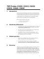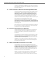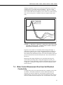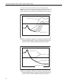
1
TDR Probes CS605, CS610,
CS630, CS635, CS640, CS645
Revision: 9/13
C o p y r i g h t © 2 0 0 6 - 2 0 1 3
C a m p b e l l S c i e n t i f i c , I n c .
Warranty
“PRODUCTS MANUFACTURED BY CAMPBELL SCIENTIFIC, INC. are
warranted by Campbell Scientific, Inc. (“Campbell”) to be free from defects in
materials and workmanship under normal use and service for twelve (12)
months from date of shipment unless otherwise specified in the corresponding
Campbell pricelist or product manual. Products not manufactured, but that are
re-sold by Campbell, are warranted only to the limits extended by the original
manufacturer. Batteries, fine-wire thermocouples, desiccant, and other
consumables have no warranty. Campbell’s obligation under this warranty is
limited to repairing or replacing (at Campbell’s option) defective products,
which shall be the sole and exclusive remedy under this warranty. The
customer shall assume all costs of removing, reinstalling, and shipping
defective products to Campbell. Campbell will return such products by surface
carrier prepaid within the continental United States of America. To all other
locations, Campbell will return such products best way CIP (Port of Entry)
INCOTERM® 2010, prepaid. This warranty shall not apply to any products
which have been subjected to modification, misuse, neglect, improper service,
accidents of nature, or shipping damage. This warranty is in lieu of all other
warranties, expressed or implied. The warranty for installation services
performed by Campbell such as programming to customer specifications,
electrical connections to products manufactured by Campbell, and product
specific training, is part of Campbell’s product warranty. CAMPBELL
EXPRESSLY DISCLAIMS AND EXCLUDES ANY IMPLIED
WARRANTIES OF MERCHANTABILITY OR FITNESS FOR A
PARTICULAR PURPOSE. Campbell is not liable for any special, indirect,
incidental, and/or consequential damages.”
Assistance
Products may not be returned without prior authorization. The following
contact information is for US and international customers residing in countries
served by Campbell Scientific, Inc. directly. Affiliate companies handle
repairs for customers within their territories. Please visit
www.campbellsci.com to determine which Campbell Scientific company serves
your country.
To obtain a Returned Materials Authorization (RMA), contact CAMPBELL
SCIENTIFIC, INC., phone (435) 227-9000. After an application engineer
determines the nature of the problem, an RMA number will be issued. Please
write this number clearly on the outside of the shipping container. Campbell
Scientific’s shipping address is:
CAMPBELL SCIENTIFIC, INC.
RMA#_____
815 West 1800 North
Logan, Utah 84321-1784
For all returns, the customer must fill out a “Statement of Product Cleanliness
and Decontamination” form and comply with the requirements specified in it.
The form is available from our web site at www.campbellsci.com/repair. A
completed form must be either emailed to [email protected] or faxed to
(435) 227-9106. Campbell Scientific is unable to process any returns until we
receive this form. If the form is not received within three days of product
receipt or is incomplete, the product will be returned to the customer at the
customer’s expense. Campbell Scientific reserves the right to refuse service on
products that were exposed to contaminants that may cause health or safety
concerns for our employees.
Table of Contents
PDF viewers: These page numbers refer to the printed version of this document. Use the
PDF reader bookmarks tab for links to specific sections.
1. Introduction .................................................................1
2. Cautionary Statements...............................................1
3. Initial Inspection .........................................................1
4. Overview......................................................................1
5. Specifications .............................................................2
5.1
5.2
5.3
Physical Description.............................................................................2
Measurement Parameters .....................................................................2
Electromagnetic Compatibility ............................................................3
6. Installation ...................................................................3
7. Operation .....................................................................3
7.1
Probe Offset for Water Content Measurement.....................................3
7.1.1 Calculating Probe Offset...............................................................3
7.2
Probe Constant for Electrical Conductivity Measurement ...................4
7.2.1 Electrical Conductivity Error from Attenuation............................4
7.3
Water Content Measurement Error from Cable ...................................4
7.4
Water Content Measurement Error from Soil Electrical
Conductivity .....................................................................................5
8. References ..................................................................7
Appendices
A. Discussion of TDR Probe Offset and a Simple
Laboratory Method for Calculation ..................... A-1
A.1
A.2
Discussion of Probe Offset.............................................................. A-1
The Compounding Effect of Signal Attenuation in Connecting
Cables .......................................................................................... A-2
A.3 Method for Calculating Probe Offset Using Information from the
Terminal Mode of PC-TDR......................................................... A-3
A.3.1 Procedure for Calculating Probe Offset ................................... A-3
A.3.2 An Example Using CS605 ....................................................... A-4
i
Table of Contents
B. Correcting Electrical Conductivity
Measurements for System Losses......................B-1
B.1
B.2
Description of Method..................................................................... B-1
Detailed Method Description........................................................... B-2
B.2.1 Collecting Reflection Coefficient with Probes Open and
Shorted.................................................................................. B-2
B.2.2 Determining Kp ........................................................................ B-2
B.2.3 Deriving Calibration Function.................................................. B-3
B.2.4 CR1000 Program for Collecting ρopen and ρshorted Values ......... B-4
7-1.
Waveforms collected in a sandy loam using CS610 probe with
RG8 connecting cable. Volumetric water content is 24% and
bulk electrical conductivity is 0.3 dS m-1......................................... 5
Waveforms collected in a sandy loam using CS610 probe with RG8
connecting cable. Volumetric water content values are 10, 16,18,
21 and 25%. Solution electrical conductivity is 1.0 dS m-1. ................. 6
Waveforms collected in a sandy loam using CS610 probe with RG8
connecting cable. Volumetric water content values are 10, 18, 26,
30 and 37%. Solution electrical conductivity is 10.2 dS m-1................. 6
Example of start of TDR probe determination ................................ A-2
Example of corrected and uncorrected electrical conductivity
values. .......................................................................................... B-3
Figures
7-2.
7-3.
A-1.
B-1.
Tables
5-1.
5-2.
A-1.
B-1.
TDR Probe Physical Properties ........................................................... 2
TDR Probe Measurement Properties ................................................... 2
Dielectric permittivity values for range of temperatures. From
equation [A5]. .............................................................................. A-5
Standard KCl Solutions ................................................................... B-2
ii
TDR Probes CS605, CS610, CS630,
CS635, CS640, CS645
1.
Introduction
This document presents descriptions and instructions for Campbell Scientific
Time Domain Reflectometry (TDR) probes and includes some TDR principles.
Consult the TDR100 operating manual for comprehensive TDR instructions.
A single TDR probe can be connected directly to the TDR100 or multiple
probes connected via the SDMX50-series Coaxial Multiplexers.
Before using the TDR probes, please study:
•
•
2.
3.
4.
Section 2, Cautionary Statements
Section 3, Initial Inspection
Cautionary Statements
•
Care should be taken when opening the shipping package to not damage or
cut the cable jacket. If damage to the cable is suspected, consult with a
Campbell Scientific application engineer.
•
The CS605 and CS610 are shipped with rubber caps covering the sharp
ends of the rods. Remove the three caps before use.
•
The TDR100 is sensitive to electrostatic discharge damage. Avoid
touching the center conductor of the panel BNC connector or the center
rod of TDR probes connected to the TDR100.
Initial Inspection
•
Upon receipt of a TDR probe, inspect the packaging and contents for
damage. File damage claims with the shipping company.
•
The model number and cable length are printed on a label at the
connection end of the cable. Check this information against the shipping
documents to ensure the correct product and cable length are received.
Overview
TDR probes are the sensors of the TDR measurement system and are inserted
or buried in the medium to be measured. The probes are a wave guide
extension on the end of coaxial cable. Reflections of the applied signal along
the waveguide will occur where there are impedance changes. The impedance
value is related to the geometrical configuration of the probe (size and spacing
of rods) and also is inversely related to the dielectric constant of the
surrounding material. A change in volumetric water content of the medium
surrounding the probe causes a change in the dielectric constant. This is seen
1
TDR Probes CS605, CS610, CS630, CS635, CS640, CS645
as a change in probe impedance which affects the shape of the reflection. The
shape of the reflection contains information used to determine water content
and soil bulk electrical conductivity.
5.
Specifications
5.1
Physical Description
TABLE 5-1. TDR Probe Physical Properties
Probe
Model
Rods
Probe Head
Cable Type
CS605
length
30.0 cm
diameter 0.475 cm
length
width
thickness
10.8 cm
7.0 cm
1.9 cm
RG58
CS610
length
30.0 cm
diameter 0.475 cm
length
width
thickness
10.8 cm
7.0 cm
1.9 cm
RG8
low loss
CS630
length
15.0 cm
diameter 0.318 cm
length
width
thickness
5.75 cm
4.0 cm
1.25 cm
RG58
CS635
length
15.0 cm
diameter 0.318 cm
length
width
thickness
5.75 cm
4.0 cm
1.25 cm
LMR-200
low loss
CS640
length
diameter
7.5 cm
0.159 cm
length
width
thickness
4.5 cm
2.2 cm
1.0 cm
RG58
CS645
length
diameter
7.5 cm
0.159 cm
length
width
thickness
4.5 cm
2.2 cm
1.0 cm
LMR-200
low loss
5.2
Maximum Soil
Bulk Electrical
Conductivity
Maximum
Cable Length
(measured from
the tips of the
probe’s rods to
the TDR100
Reflectometer)
1.4 dS/m
15 m
1.4 dS/m
25 m
3.5 dS/m
15 m
3.5 dS/m
25 m
5.0 dS/m
15 m
5.0 dS/m
25 m
Measurement Parameters
TABLE 5-2. TDR Probe Measurement Properties
2
Probe Model
Probe Offset
(meters)
Probe Constant for Electrical
Conductivity (EC) Measurement, Kp
(using this constant will provide EC in
siemens/meter)
CS605 and CS610
0.090
1.74
CS630 and CS635
0.052
3.36
CS640 and CS645
0.035
6.40
TDR Probes CS605, CS610, CS630, CS635, CS640, CS645
5.3
Electromagnetic Compatibility
All TDR probes are
compliant with performance criteria available upon
request. RF emissions are below EN55022 limit.
6.
Installation
TDR probes can be installed in any orientation: horizontally, vertically, or at an
angle to the surface. The measured water content is the integral or average of
the water content over the length of the probe rods. The probe rods should be
completely surrounded by the soil or other media being measured. If portions
of the probe rods are exposed to air, the algorithm for analyzing the waveform
reflection may not be able to correctly locate the beginning and end of the
probe rods.
Care must be exercised when inserting probe rods into the soil to minimize soil
compaction around the rods. Compaction can leave air voids along the length
of the rods. The region adjacent to the rod is the most sensitive so voids near
the rods can be a significant source of error.
After the soil is disturbed for probe installation, most soils will experience
rejuvenation of the soil structure with wetting/drying cycle and freeze/thaw
cycles.
TDR probes can be buried or inserted into the soil. The CS605G Installation
Guide should be used when inserting the CS605 and CS610 into the material
being measured. A guide is generally not needed for the smaller diameter
probes.
7.
Operation
7.1
Probe Offset for Water Content Measurement
A portion of the TDR probe rods is surrounded by the probe head material and
is not exposed to the material being measured. Probe offset is used to correct
for this. TABLE 5-2 lists offset values for probes manufactured by Campbell
Scientific. These values are entered in the datalogger instruction or in the PCTDR software.
7.1.1 Calculating Probe Offset
Probe offset can be calculated using information from PC-TDR. The probe
rods are immersed in water of known temperature, algorithm values are
collected in the terminal emulator mode of PC-TDR, and simple calculations
provide custom offset values. See Appendix A, Discussion of TDR Probe
Offset and a Simple Laboratory Method for Calculation, for calculation
method.
The values listed in TABLE 5-2 were determined using TDR probes with short
cables. The shape of the waveform reflection is affected as cable length
increases, and this can introduce error into the water content measurement.
Using probe offsets determined by the method described in Appendix A,
Discussion of TDR Probe Offset and a Simple Laboratory Method for
3
TDR Probes CS605, CS610, CS630, CS635, CS640, CS645
Calculation, with all cabling from TDR100 to probe in place will compensate
for the cable losses. Probe offset values obtained this way will be greater than
those listed in TABLE 5-2.
7.2
Probe Constant for Electrical Conductivity Measurement
The electrical conductivity measurement requires a probe constant to account
for probe geometry. The probe constant is commonly referred as Kp. The
probe constant is entered as a multiplier in the datalogger instruction for
TDR100 EC measurement. Kp is set in PC-TDR using Settings/Calibration
Functions/Bulk Electrical Conductivity. Using the Kp values in TABLE 5-2
will give electrical conductivity in the units siemens/meter. For the more
common units of decisiemens/meter, multiply the TABLE 5-2 Kp values by 10.
Probe constant can be calculated using PC-TDR. Selecting
Settings/Calibration Functions/Bulk Electrical Conductivity will present a
button to Measure Cell Constant. The method requires submersion of the TDR
probe rods in de-ionized water of known temperature. See PC-TDR HELP for
simple instructions. It is recommended to make several Kp determinations and
use the average value.
Probe constant can also be calculated using the method presented in Appendix
B, Correcting Electrical Conductivity Measurements. This method accounts
for signal losses in system cabling and multiplexers.
7.2.1 Electrical Conductivity Error from Attenuation
Attenuation of the applied and reflected signal in the cable and multiplexers
will affect the accuracy of the electrical conductivity measurement. For
accurate electrical conductivity measurements, this attenuation must be
accounted for.
A paper published by Castiglione and Shouse (2003) describes the error and a
method to account for the error. The method requires electrical conductivity
measurement with the probes in air and with the rods shorted with all system
components in place (cable and multiplexers).
Appendix B, Correcting Electrical Conductivity Measurements, presents a
summary of the Castiglione and Shouse (2003) method and an adaptation of
the method for the TDR100 system.
7.3
Water Content Measurement Error from Cable
The determination of water content using the TDR system relies on the
evaluation of a pulse reflection from the TDR probe. The pulse generated by
the TDR100 and its reflections are subject to distortion during travel between
the TDR100 and the TDR probe. The cable connecting the probe to the
reflectometer has a characteristic impedance resulting in both resistive and
reactive losses. Distortion of the waveform caused by cable impedance can
introduce error into the water content determination.
FIGURE 7-1 presents waveforms collected from a 3-rod probe (CS610) for
various cable lengths. As cable length increases, the rise time and the
amplitude of the reflection are affected. The slopes and extrema used by the
4
TDR Probes CS605, CS610, CS630, CS635, CS640, CS645
datalogger algorithm to analyze the waveform are shifted by the cable losses
resulting in error. For the data shown in FIGURE 7-1, the water content
measurement using the 66 meter cable was in error by about 1.5% volumetric
water content when electrical conductivity is low. However, in saline soils, the
error can be several percent. See Bilskie (1997) for complete results of the
study.
16 meter cable
26 meter cable
45 meter cable
66 meter cable
FIGURE 7-1. Waveforms collected in a sandy loam using CS610 probe
with RG8 connecting cable. Volumetric water content is 24% and
bulk electrical conductivity is 0.3 dS m-1.
In general, water content is overestimated with increasing cable length. A
calibration of volumetric water content with apparent dielectric constant for a
given cable length can improve accuracy. Measurement precision at longer
cable lengths will be maintained as long as soil electrical conductivity does not
prevent a reflection from the end of the probe rods. This is discussed later in
this section.
Minimizing cable lengths should always be considered in the design of a
measurement system using TDR. If long cable lengths are necessary, the
adverse effects can be minimized by using low attenuation cable such as RG8
or LMR-200. Careful probe design ensures correct probe impedance giving
robust reflections.
7.4
Water Content Measurement Error from Soil Electrical
Conductivity
The signal at the probe will be attenuated when ionic conduction occurs in the
soil solution. This inherent attenuation is used in TDR measurements to
determine soil electrical conductivity as described by equation [5] in the
TDR100 manual. The presence of ions in the soil solution provides a path for
electrical conduction between TDR probe rods. The attenuation of the signal
5
TDR Probes CS605, CS610, CS630, CS635, CS640, CS645
can affect the accuracy and resolution of water content measurements.
FIGURE 7-2 presents a series of waveforms when a solution with an electrical
conductivity of 1.0 dS m-1 is added to a soil which has essentially no salt
present. FIGURE 7-3 shows data for solution with high electrical conductivity.
water content = 9.5%
water content = 25%
FIGURE 7-2. Waveforms collected in a sandy loam using CS610 probe
with RG8 connecting cable. Volumetric water content values are 10,
16,18, 21 and 25%. Solution electrical conductivity is 1.0 dS m-1.
water content = 18%
water content = 37%
FIGURE 7-3. Waveforms collected in a sandy loam using CS610 probe
with RG8 connecting cable. Volumetric water content values are 10,
18, 26, 30 and 37%. Solution electrical conductivity is 10.2 dS m-1.
6
TDR Probes CS605, CS610, CS630, CS635, CS640, CS645
The combined effect of long cable runs and high soil electrical conductivity
must be considered when TDR measurements are taken.
8.
References
Bilskie, Jim. 1997. “Reducing Measurement Errors of Selected Soil Water
Sensors.” Proceedings of the International Workshop on Characterization and
measurement of the hydraulic properties of unsaturated porous media. 387396.
Castiglione, P. and P.J. Shouse. 2003. The effect of ohmic cable losses on
time-domain reflectometry measurements of electrical conductivity. Soil Sci
Soc Am J 2003 67: 414-424.
7
TDR Probes CS605, CS610, CS630, CS635, CS640, CS645
8
Appendix A. Discussion of TDR Probe
Offset and a Simple Laboratory Method
for Calculation
A.1 Discussion of Probe Offset
Probe offset accounts for the segment of the TDR probe rods that is part of the
probe head and is not exposed to the media surrounding the probe rods. The
location of the beginning of the probe that is calculated in the TDR100
operating system is the point along the cable where the transition from the 50
ohm cable to the TDR probe impedance occurs. The distance from this
transition to the point where the rods come out of the probe head is constant
and can be accounted for.
The TDR100 operating system uses the following equation to calculate the
ratio of apparent rod length to actual rod length, La/L. This ratio is equal to the
square root of dielectric permittivity,
La
=
L
ε.
end − start
− ProbeOff
Vp
L
La
apparent length (m)
L
actual rod length (m)
Vp
relative propagation velocity (1.0)
ProbeOff
probe offset (m)
start
distance into window for beginning of rods (m)
end
distance into window for end of rods (m)
[A1]
To examine the sensitivity of La/L to probe offset, multiply equation [A1] by L
and take the 1st derivative of La with respect to probe offset.
⎛ end − start
⎞
d
⎜
− ProbeOff ⎟ = −1
⎟
d(ProbeOff) ⎜⎝
Vp
⎠
[A2]
The sensitivity of the apparent length measurement, La, is directly related to
probe offset. A probe offset difference of 0.005 changes La by –0.005. The
water content error for saturated soil is 0.16% volumetric water content. In
very dry soil the error is 0.20%. There is a slight dependence of probe offset
on water content but the amount is within the resolution of the water content
measurement.
A-1
Appendix A. Discussion of TDR Probe Offset and a Simple Laboratory Method for Calculation
A.2 The Compounding Effect of Signal Attenuation in
Connecting Cables
The probe offset values provided in the operating manual were calculated from
measurements in the Campbell Scientific soils laboratory. The method is
described below. The length of cable for the laboratory calculations was 3
meters or less. As cable length increases, signal loss occurs in both amplitude
and bandwidth. As a result of bandwidth loss, the slope of the waveform at the
beginning of the probe decreases with increasing cable length. The probe start
is determined from the intersection of a line tangent to the waveform at the
steepest point and of a line that is essentially horizontal. See FIGURE A-1.
The probe offset correction identifies the location where the rods exit the probe
head.
calculated and corrected start
0.4
reflection coefficient
indexstartindexstartcorr
0.2
15
20
25
30
35
40
0.2
0.4
data point
horizontal line
waveform
tangent line
FIGURE A-1. Example of start of TDR probe determination
The slope of the tangent line decreases as cable length increases, and the
intersection of the two lines will shift in the direction of greater apparent probe
rod length.
Calculating the probe offset using the method described below and with all
cables and multiplexers in place will optimize the accuracy of water content
measurements.
A-2
Appendix A. Discussion of TDR Probe Offset and a Simple Laboratory Method for Calculation
A.3 Method for Calculating Probe Offset Using
Information from the Terminal Mode of PC-TDR
Letting Vp = 1 and solving [1] for ProbeOffset gives:
ProbeOff = end − start − La
[A3]
The start and end distance values are determined by an algorithm in the
TDR100 operating system. The apparent length, La, excluding the offset, is
related to actual rod length and permittivity by:
La := L • ε(T )
[A4]
The rod length, L, is the physical length of the rods (m). For 3-rod TDR
probes with longer outer rods, the length of the outer rods is used.
The dielectric permittivity of water can be calculated from water temperature
using:
[
ε (T ) := 78.54 • 1 − 4.5791 • 10 −3 • (T − 25 ) + 1.19 • 10 −5 • (T − 25 )2 − 2.8 • 10 −8 • (T − 25 )3
]
[A5]
TABLE A-1 contains dielectric permittivities for a typical range of
temperatures and may be used in lieu of equation [A5]. Substituting the
calculation of La using equations [A4] and [A5] into equation [A3] leaves the
end and start distances as the only unknowns. These values can be acquired
directly from the TDR100 algorithm by using the terminal emulator mode of
PC-TDR.
A.3.1 Procedure for Calculating Probe Offset
Connect all cabling and multiplexers to be used for field or laboratory
measurements.
Immerse the TDR probe rods in DI or tap water. The container must be large
enough to ensure rods are at least 5 cm from container walls.
Use PC-TDR as follows:
1.
Enter values for Waveform parameters. Suggested values are: Average =
4, Points = 251. Relative propagation velocity, Vp, must be 1. Choice of
start point and waveform length depends on the length of the cable and the
actual probe rod length. There should be about 0.5 meters before the
probe, enough distance for probe apparent length in water (approximately
9 times rod length), and enough distance for the waveform past the end of
the probe. The distance for the end can be approximated as 3 times rod
length.
2.
Enter the value for Probe Rod Length in meters and set Probe Offset to 0
m.
3.
Click the Water Content button to send the values to the TDR100 and to
have it calculate La/L and provide start and end values.
A-3
Appendix A. Discussion of TDR Probe Offset and a Simple Laboratory Method for Calculation
4.
Enter Terminal Mode using Options/Terminal Emulator.
5.
Press Enter until > appears
6.
Type GVAR then Enter.
7.
It is recommended that step 6 be repeated several times and that the
average values of Start and End be used for following calculations.
(the line commands are not case sensitive)
GVAR returns the uncorrected Start and End. These values must be
converted to distance from index values. This is done as follows:
start distance :=
start
• WaveformLength
datapoints − 1
end distance :=
end
• WaveformLength
datapoints − 1
Equations [A3] and [A4] are then used to calculate probe offset.
A.3.2 An Example Using CS605
•
Measured TDR probe rod length: L := 0.3 m.
•
Measure temperature of water in column T := 24.4°C .
•
Determine actual dielectric permittivity of water using following equation
or values in TABLE A-1.
ε(T ) := 78.54 • ⎡1 − 4.5791 •10 − • (T − 25) + 1.19 •10 −5 • (T − 25)2 − 2.8 •10 −8 • (T − 25)3 ⎤
⎢⎣
⎥⎦
3
ε(T ) = 78.76
La := L • ε(T )
La = 2.66 m
•
Waveform parameters for PC-TDR
WindowLength := 5 m
datapoints := 251
Probe length = 0.3 m Probe offset = 0 m
•
Start and end index values from terminal emulator mode of PC-TDR as
described above
start index := 32.44
•
end index := 169.87
converting waveform index to apparent distance
start distance :=
A-4
Vp := 1.0
start index
• WindowLength
datapoints − 1
Appendix A. Discussion of TDR Probe Offset and a Simple Laboratory Method for Calculation
end distance :=
end index
• WindowLength
datapoints − 1
start distance = 0.65
Pr obeOffset :=
end distance = 3.4
(
− La • Vp − end distance + start distance
)
Vp
ProbeOffset = 0.086
TABLE A-1. Dielectric permittivity
values for range of temperatures.
From equation [A5].
Temperature (°C)
Dielectric
Permittivity
15
82.23
15.5
82.04
16
81.85
16.5
81.67
17
81.48
17.5
81.29
18
81.1
18.5
80.92
19
80.73
19.5
80.55
20
80.36
20.5
80.18
21
79.99
21.5
79.81
22
79.63
22.5
79.44
23
79.26
23.5
79.08
24
78.9
24.5
78.72
25
78.54
25.5
78.36
26
78.18
26.5
78
A-5
Appendix A. Discussion of TDR Probe Offset and a Simple Laboratory Method for Calculation
TABLE A-1. Dielectric permittivity
values for range of temperatures.
From equation [A5].
A-6
Temperature (°C)
Dielectric
Permittivity
27
77.82
27.5
77.65
28
77.47
28.5
77.29
29
77.12
29.5
76.94
30
76.76
Appendix B. Correcting Electrical
Conductivity Measurements for System
Losses
TDR system cabling and multiplexers introduce losses of the applied and
reflected signals which can lead to error in measurement of electrical
conductivity. The following information is based on a method presented in
paper published by Castiglione and Shouse (2003). The method has been
tested by Campbell Scientific and found to provide excellent results.
Refinement of the method is provided to allow implementation using Campbell
Scientific dataloggers and TDR100 system.
B.1 Description of Method
The method is essentially a calibration and involves collecting system
characterization measurements with all system components in place; TDR100,
multiplexers, all cabling, and probes. The steps in the process are:
1.
measure reflection coefficient with probe rods open and with probe rods
shorted
2.
determine probe constant, Kp, using one solution of known electrical
conductivity
3.
use values collected in above steps to generate simple function to correct
EC measurements
4.
incorporate calibration function in datalogger program.
The method defines corrected reflection coefficient, ρcorrected, using the equation
⎛ ρ uncorrected − ρ open
ρ corrected = 2⎜
⎜ ρ open − ρ shorted
⎝
⎞
⎟ +1
⎟
⎠
[B1]
ρcorrected is then used to determine the conductance, G, with a TDR probe rods
immersed in a solution of known electrical conductivity. ρuncorrected is the
refection coefficient at distance 200 m (example given below). The equation
for conductance is:
⎛ 1
G = ⎜⎜
⎝ Zu
⎞ ⎛ 1 − ρ corrected
⎟⎜
⎟ ⎜1+ ρ
corrected
⎠⎝
⎞
⎟
⎟
⎠
[B2]
with Zu the system impedance, 50 ohms.
Kp is the slope of a graph of electrical conductivity versus electrical
conductance, σ = K p G . Since this function passes through the origin, only
one measurement of G is needed with a probe immersed in a solution of known
B-1
Appendix B. Correcting Electrical Conductivity Measurements for System Losses
electrical conductivity. Kp is calculated as the ratio of electrical conductivity to
electrical conductance and presented in equation [B3].
Kp =
σ
G
[B3]
With Kp determined, a calibration equation can be derived that corrects EC
measurements for system losses.
B.2 Detailed Method Description
B.2.1 Collecting Reflection Coefficient with Probes Open and
Shorted
The EC measurement is independent of frequency and uses reflection
coefficient values from locations well after probe reflections have stabilized. A
distance of 200 meters is chosen for the measurement.
The ρopen value is collected with the probe suspended in air. The ρshorted value
is collected with the end of the probe rods shorted while suspended in air. ρopen
and ρshorted values are easily determined using PC-TDR. Set waveform
parameters to:
Average = 4
Points = 20
Start = 200
Length = 1.
Click Get Waveform and adjust graph scale using the Adjust Axes Range button
to allow determination of reflection coefficient to nearest 0.005.
ρopen and ρshorted values can also be collected using a datalogger. See Section
B.2.4 , CR1000 Program for Collecting ρopen and ρshorted Values, for CR1000
datalogger program that can be used to collect ρopen and ρshorted values.
B.2.2 Determining Kp
Kp is the slope of electrical conductivity, σ, as a function of conductance, G.
Completely immerse the probe rods in a solution of known or measured
electrical conductivity. TABLE B-1 provides KCl amounts for a range of
solution electrical conductivities. Since σ is zero when G is zero, Kp is simply
the ratio of the known or measured electrical conductivity to the conductance,
G, measured using equations [B3] and [B1].
TABLE B-1. Standard KCl Solutions
B-2
Electrical Conductivity @ 25°C
(decisiemens/meter)
Grams of KCl/liter of solution
111.34
74.2460
12.86
7.4365
1.409
0.7440
0.147
0.0744
Appendix B. Correcting Electrical Conductivity Measurements for System Losses
The temperature effect is described by:
EC T = EC 25 • (1 + 0.02 • (T − 25))
[B4]
where EC 25 is the electrical conductivity at 25ºC and EC T is the electrical
conductivity at other temperatures.
B.2.3 Deriving Calibration Function
Using the Kp, ρopen and ρshorted values for each probe, the uncorrected electrical
conductivity as measured by the TDR100 can be corrected to give accurate EC
values that account for system losses. To do this, a range of EC values is
chosen for σuncorrected in equation [B5] and σcorrected values calculated for the
chosen range of σuncorrected.
(
σ uncorrected • Z u − K p + ρ air • σ uncorrected • Z u + ρ air • K p
Z u ρ shorted • σ uncorrected • Z u + ρ shorted • K p + σ uncorrected • Z u − K p
)
[B5]
This equation has a quadratic form. The correction is easier to use if a curve is
fit to the σcorrected values for the chosen range of σuncorrected. This quadratic is
implemented in the datalogger program to given the final result that is
corrected electrical conductivity. This must be done for each probe.
corrected EC (siemen/meter)
σ corrected = −K p •
1.5
0.75
0
0
0.75
1.5
uncorrected EC (siemen/meter)
FIGURE B-1. Example of corrected and uncorrected electrical
conductivity values.
The fitted equation for this probe is
σ corrected = 0.01 + 0.95 • σ uncorrected + 0.35 • σ uncorrected 2
B-3
Appendix B. Correcting Electrical Conductivity Measurements for System Losses
B.2.4 CR1000 Program for Collecting ρopen and ρshorted Values
'This example program is written for 4 TDR probes connected to
'a single multiplexer. It will be necessary to add instructions in
'subroutine TDR if more probes are used.
'CR1000 Series Datalogger
'Declare Public & Dim Variables
Public wave(30), vector(20)
Public rho(2)
Public channel as long
Public Open as boolean
Public Shorted as boolean
Public SDMports as boolean
Public WriteToOutput as boolean
Dim I
'Declare Constants
'Flag logic constants
const high = true
const low = false
'Define Data Tables
DataTable (rhoTable,1,-1)
Sample(1,channel,Long)
Sample (2,rho(),IEEE4)
EndTable
‘
sub TDR
'set multiplexer address code for specific system
Select Case channel
Case 1
TDR100 (wave(),0,1,1001,4,1.0,20,200,1.0,0.075,0.0,1,0)
Case 2
TDR100 (wave(),0,1,2001,4,1.0,20,200,1.0,0.075,0.0,1,0)
Case 3
TDR100 (wave(),0,1,3001,4,1.0,20,200,1.0,0.075,0.0,1,0)
Case 4
TDR100 (wave(),0,1,4001,4,1.0,20,200,1.0,0.075,0.0,1,0)
EndSelect
endsub
'Main Program
BeginProg
Scan (5,sec,0,0)
if Open=high then
TDR
For I=1 To 20
vector(I)=wave(I+9)
Next
AvgSpa (rho(1),20,vector(1))
Open=low
endif
if Shorted=high then
TDR
For I=1 To 20
vector(I)=wave(I+9)
Next
AvgSpa (rho(2),20,vector(1))
Shorted=low
endif
'write results to output storage
If WriteToOutput=high Then
CallTable rhoTable
WriteToOutput=low
EndIf
B-4
Appendix B. Correcting Electrical Conductivity Measurements for System Losses
'setting SDMports high will configure control ports 1 thru 3 to allow connection
'of TDR100 to PC using PC-TDR
If SDMports=high Then
PortsConfig (&B00000111,&B00000000)
SDMports=low
EndIf
NextScan
EndProg
B-5
Appendix B. Correcting Electrical Conductivity Measurements for System Losses
B-6
Campbell Scientific Companies
Campbell Scientific, Inc. (CSI)
815 West 1800 North
Logan, Utah 84321
UNITED STATES
www.campbellsci.com • [email protected]
Campbell Scientific Africa Pty. Ltd. (CSAf)
PO Box 2450
Somerset West 7129
SOUTH AFRICA
www.csafrica.co.za • [email protected]
Campbell Scientific Australia Pty. Ltd. (CSA)
PO Box 8108
Garbutt Post Shop QLD 4814
AUSTRALIA
www.campbellsci.com.au • [email protected]
Campbell Scientific do Brasil Ltda. (CSB)
Rua Apinagés, nbr. 2018 ─ Perdizes
CEP: 01258-00 ─ São Paulo ─ SP
BRASIL
www.campbellsci.com.br • [email protected]
Campbell Scientific Canada Corp. (CSC)
11564 - 149th Street NW
Edmonton, Alberta T5M 1W7
CANADA
www.campbellsci.ca • [email protected]
Campbell Scientific Centro Caribe S.A. (CSCC)
300 N Cementerio, Edificio Breller
Santo Domingo, Heredia 40305
COSTA RICA
www.campbellsci.cc • [email protected]
Campbell Scientific Ltd. (CSL)
Campbell Park
80 Hathern Road
Shepshed, Loughborough LE12 9GX
UNITED KINGDOM
www.campbellsci.co.uk • [email protected]
Campbell Scientific Ltd. (CSL France)
3 Avenue de la Division Leclerc
92160 ANTONY
FRANCE
www.campbellsci.fr • [email protected]
Campbell Scientific Ltd. (CSL Germany)
Fahrenheitstraße 13
28359 Bremen
GERMANY
www.campbellsci.de • [email protected]
Campbell Scientific Spain, S. L. (CSL Spain)
Avda. Pompeu Fabra 7-9, local 1
08024 Barcelona
SPAIN
www.campbellsci.es • [email protected]
Please visit www.campbellsci.com to obtain contact information for your local US or international representative.