Download Alpes Lasers . TC-3 Datasheet

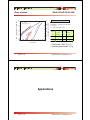
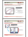
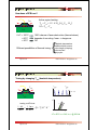
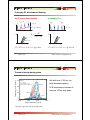
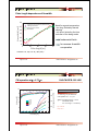
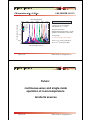
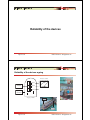
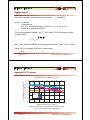
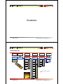
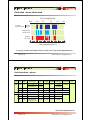
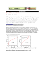
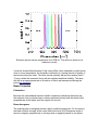
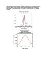
Boston Electronics Corporation
91 Boylston Street, Brookline, Massachusetts 02445 USA
(800)347-5445 or (617)566-3821 fax (617)731-0935
www.boselec.com
[email protected]
Room Temperature
TUNABLE
IR DIODE LASERS
from
Alpes Lasers
Readily available:
Single Mode many devices between 4.3 and 10.4 µm
Multimode 5.0 to 6.2 and 8.5 to 10.6 µm
Built to order:
3.5 to >90 µm
3.5
3
2.5
2
1.5
1
0.5
Alpes #sb9 at different temps with different drive
voltages
-30C
nm
0C
4/8/2004
+30C
Boston Electronics
(800)347-5445 or [email protected]
0
10342 10347 10352 10364 10368 10373 10387 10391 10394
lambda vs T and V Chart 2
mW average, 2% duty cycle
High power and single frequency quantum
cascade lasers for chemical sensing
Stéphane Blaser
final version: http://www.alpeslasers.ch/Conference-papers/QCLworkshop03.pdf
Page 1 of 51
Boston Electronics * [email protected]
Collaborators
Yargo Bonetti
Lubos Hvozdara
Antoine Muller
Guillaume Vandeputte
Hege Andersen
This work was done in collaboration
with the University of Neuchâtel
Page 2 of 51
Marcella Giovannini
Nicolas Hoyler
Mattias Beck
Jérome Faist
Boston Electronics * [email protected]
Outline
• Company profile
• Introduction - state of the art
– High power Fabry-Pérot devices
• Applications
• Distributed-feedback lasers
– High power pulsed DFB devices
– >77K operating continuous-wave DFB devices
• Reliability
• Production
Page 3 of 51
Boston Electronics * [email protected]
Company profile
• Founded August 1998 as a spin-off company from the
University of Neuchâtel
– incorporated as a SA under swiss law with a capital of 100 kCHF)
• Founders
– Jérôme Faist
– Antoine Muller
– Mattias Beck
• Employees (September 2003)
– 8 persons (6 full-time)
Installed at Maximilien-de-Meuron 1-3,
2000 Neuchâtel since April 2002
Page 4 of 51
Boston Electronics * [email protected]
Company profile
• > 30 man-years experience
• 7 patents on QCL technologies
• > 150 devices sold
• > 50 customers
• turnover 2003: > 1.3 MCHF
• average growth rate: 100% / year
Page 5 of 51
Boston Electronics * [email protected]
Quantum cascade lasers
Page 6 of 51
Boston Electronics * [email protected]
Interband vs intersubband
E
E
Ef
Ef
E12
E12
k||
k||
• Interband transition
- bipolar
- photon energy limited by bandgap
Eg of material
- Telecom, CD, DVD,…
• Intersubband transition
- unipolar, narrow gain
- photon energy depends on layer
thickness and can be tailored
Page 7 of 51
Boston Electronics * [email protected]
Quantum cascade lasers
• Cascade
- each e- emits N photons
• Active region / injector
- active region ¨ population inversion which
must be engineered
- injector ¨ avoid fields domains and cools
down the electrons
• MBE
- growth of thin layers
- sharp interfaces
Te>>Tl
3
τ32 > τ21
2
1
τ32
τ21 Te~Tl
active region relaxation / injection
Page 8 of 51
Boston Electronics * [email protected]
State of the art: QCL performances
Atmospheric windows
Reststrahlen band
Temperature [K]
150
Peltier
LN2
0
2
5
10
20
50
100
CW
pulsed
678
300
CW
pulsed
678
450
InP
GaAs
- Good Mid-IR coverage
- Terahertz promising
Data:
MIR
FIR
Uni Neuchâtel
NEST Pisa
Alpes Lasers
MIT
Bell Labs
Uni Neuchâtel
Thales
TU Vienna
Northwestern Uni
W. Schottky/TU Munich
Wavelength [µm]
Page 9 of 51
Boston Electronics * [email protected]
Designs
Double-phonon resonance:
(patent n° wo 02/23686A1)
• 4QW active region with 3 coupled lower state
• lower states separated by one phonon energy each
• keeps good injection efficiency of the 3QW design
Hofstetter et al. APL 78, 396 (2001).
Double optical phonon
resonance
Bound-to-continuum:
(patent n° wo 02/019485A1)
• transition from a bound state to a miniband
• combines injection and extraction efficiency
• broad gain curve -> good long-wavelength and
high temperature operation
J. Faist et al. APL 78, 147 (2001).
Page 10 of 51
Bound-to-continuum
Boston Electronics * [email protected]
Two-phonon structure at 8 Pm
injection barrier
arrow QW/barrier pair
Based on two-phonon
resonances design
extraction barrier
InGaAs/InAlAs-based
heterostructure with 'Ec = 0.52eV
Grown by MBE on InP substrate
35 periods
n-d
ope
d
4Q
Wa
ctiv
e
reg
i
on
one
per
iod
41, 16, 8, 53, 10, 52, 11, 45, 21, 29, 15, 28, 16, 28, 17, 27, 18, 25, 21, 25, 26, 24, 29, 24
Page 11 of 51
Boston Electronics * [email protected]
RT-HP-FP-150-1266
16
0.9
14
0.8
96K, 60%
300K, 20%
12
0.7
0.6
10
2.5 mm-long
28 µm-wide
back-facet coated
8
6
0.5
0.4
0.3
4
0.2
2
0.1
0
0
0.5
1.0
1.5
2.0
2.5
3.0
3.5
4.0
0
4.5
Characteristics
Average power [W]
Voltage [V]
High average power FP QCL
λ = 7.9 µm
@300K: Average power:
P = 150 mW
threshold current:
Ith = 2.1A (jth=3.0 kA/cm2)
@96K : P = 0.82 W (60% dc)
Ith = 0.51A (jth=0.75 kA/cm2)
CW: P = 300mW
(jth = 0.78 kA/cm2)
Current [A]
Page 12 of 51
Boston Electronics * [email protected]
Array of lasers
DUAL-RT-HP-FP-40-1266
50
0
1
2
er
dn
5
arr
ay
of
2
30
20
las
ru
p
10
3
4
Current [A]
10
5
6
7
0
Characteristics
Average power [mW]
las
e
15
0
40
rs
T = -25°C
duty-cycle = 10%
las
e
DC voltage fed to LDD [V]
20
both lasers: 1.5 mm-long, 28 µm-wide
λ ≈ 7.9 µm
T = -25°C, duty-cyle = 10%
j th
laser
Average
power
I th [A]
up
25.4 mW
1.8
4.29
dn
22.6 mW
1.6
3.81
array
44.9 mW
3.4
4.05
[kA/cm
2
]
• Total power § 90% (P1+P2)
• Total threshold current § I1+I2
Page 13 of 51
Boston Electronics * [email protected]
Applications
Page 14 of 51
Boston Electronics * [email protected]
Applications: telecom
• Telecommunications
– Free-space optical data transmission for the last mile
(high speed with no need for licence and better operation
in fog, compared to O = 1.55 Pm)
4 to 7 years
100 Gbps
40 Gbps
1 to 4 years
Bandwidth
10 Gbps
Present
1 Gbps
622 Mbps
155 Mbps
1 Mbps
Local
Network
Last Mile
Metro Backbone
Long-Haul Backbone
R. Martini et al., IEE Elect. Lett. 37 (11), p. 1290, 2001.
S. Blaser et al., IEE Elect. Lett. 37 (12), p. 778, 2001.
Page 15 of 51
Boston Electronics * [email protected]
Main application: chemical sensing by optical spectroscopy
Detection techniques already demonstrated using QCL:
•
photo-acoustic
–
–
–
•
B. Paldus et al., Opt. Lett. 25 (9), p. 666, 2000.
single mode
A. Kosterev et al., Appl. Phys. B 75 (2-3), p. 351, 2002.
heterodyne detection scheme
–
•
high-power laser
absorption spectroscopy
–
•
M. Zahniser et al. (Aerodyne Research), TDLS’03.
cavity ringdown
–
•
Some needs:
TILDAS
•
•
B. Paldus et al., Opt. Lett. 24 (3), p.178, 1999.
D. Hofstetter et al., Opt. Lett. 26 (12), p. 887, 2001.
M. Nägele et al., Analytical Sciences 17 (4), p. 497, 2001.
continuous-wave
D. Weidmann et al., Opt. Lett. 29 (9), p. 704, 2003.
cavity enhanced spectroscopy
•
D. Bear et al. (Los Gatos Research), TDLS’03.
Page 16 of 51
Boston Electronics * [email protected]
Application fields
•
Chemical sensing or trace gas measurements
–
–
–
–
–
•
process development
environmental science
forensic science
process gas control
liquid detection spectroscopy
Medical diagnostics
– breath analyzer
– glucose dosage
•
Remote sensing
– leak detection
– exhaust plume measurement
– combat gas detection
Page 17 of 51
Boston Electronics * [email protected]
Simultaneous 3-gas measurements with dual-laser QCL instrument
NH3 (5 ppb)
LASER 1: 967 cm-1
8
4
0
-4
310
305
300
295
290
N2O (310 ppb)
TRACTOR
EXHAUST
PLUME
LASER 2: 1271 cm-1
1880
1840
CH4 (1800 ppb)
1800
Two QC-lasers from Alpes:
2 to 6 gases (CH4, N2O, NH3)
56 m cell path length
Detector options
1760
1800
12:45 PM
8/13/2003
12:50 PM
12:55 PM
1:00 PM
time
M. Zahniser et al.,
Aerodyne Research Inc., Billerica (USA)
Page 18 of 51
Boston Electronics * [email protected]
0.4 µm
0.8 µm
10 µm
infrared
UV
QCL
CO2 laser
100 µm
10 THz
NH3 maser
RADAR
0.1 THz
radio
p-Ge laser
1 mm
1 cm
10 cm
Spectrum covered by Alpes Lasers dfb QCLs
Wavelength [µm]
10.0
7.0
5.0
4.0
3.0
500
1000
1500
2000
CO2
CO
N2O
CCl2O
C5H10O
C2H4
N2O
CH4
NH3
F4Si
O3
CCl2O2
C2H4O
20.0
2500
Wavenumber [cm-1]
Page 19 of 51
Boston Electronics * [email protected]
Single-mode operation:
distributed-feedback QCLs
Page 20 of 51
Boston Electronics * [email protected]
3000
How does a DFB work?
gain
DFB:
periodic grating => waves coupling
=> high wavelength
selectivity
gain
complex-coupled DFB:
• lasing mode closest to the stopband
• stopband § coupling strength
Page 21 of 51
Amplified light bounces
in the cavity
Wavelength [µm]
9.1
9
8.9
8.8
stopband
∆ν = 1.19 cm-1
180 K
Intensity [a.u.]
Fabry-Pérot
laser:
200 K
220 K
1095 1100 1105 1110 1115 1120 1125 1130 1135 1140
Frequency [cm-1]
Boston Electronics * [email protected]
Distributed-feedback technologies
D. Hofstetter et al., Appl. Phys. Lett.,
vol. 75, p.665, 1999)
C. Gmachl et al. IEEE Photon.
Technol. Lett., vol. 9, p.1090, 1997)
Grating on the surface (open-top)
Grating close to active region
• one MBE run (no MOCVD)
• high peak power (large stripes)
but low average power
• optical losses due to metalization
• lower thermal resistance
(high duty / high temperature)
• high average power
• higher overlap, smaller losses
• jct dn mounting possible
• needs MOCVD regrowth
Page 22 of 51
Boston Electronics * [email protected]
High average power DFB QCL
RT-HP-DFB-20-1200
Distributed feedback QC laser at 8.35Pm with InP top cladding
35
30
Voltage [V]
8
25
6
-30°C
20
0°C
15
4
30°C
10
2
0
5
0
1
2
3
4
5
6
7
Characteristics
Average power [mW]
10
3mm-long, 28µm-wide laser
λ ≈ 8.35 µm
@-30°C: Average power (2% dc):
P = 32 mW (1.6 W peak power)
threshold current:
Ith = 2.44 A (jth = 2.9 kA/cm2)
@30°C : P = 25 mW (1.25W peak power)
Ith = 3.2 A (jth = 3.8 kA/cm2)
0
Current [A]
Page 23 of 51
Boston Electronics * [email protected]
High average power DFB QCL
35
30
Voltage [V]
8
-30°C
25
0°C
6
20
30°C
15
4
10
2
0
5
0
1
2
3
4
Current [A]
5
6
7
0
Characteristics
Average power [mW]
10
RT-HP-DFB-20-1200
Entire tuning range:
∆ν = 5.7 cm-1 at 1197 cm-1 (0.47%)
(1195.2 cm-1 (8.367 µm) at 30°C to 1200.9 cm-1 (8.327 µm) at -30°C)
1
0.1
0.01
0°C
30°C
30°C, 14V
30°C, 12V
15°C, 14V
15°C, 12V
0°C, 14V
0°C, 12V
40 dB (limited by the
grating spectrometer)
0.001
0.0001
8.30
8.32
8.34
8.36
8.38
8.40
Wavelength [µm]
Page 24 of 51
Boston Electronics * [email protected]
RT-P-DFB-1-608
Long-wavelength (O§16.4Pm) B2C DFB QCL
Laser based on a bound to continuum design, O§ 16.4 Pm
Rochat et al., APL 79, 4271 (2001)
1.6
30
1.4
-30°C
-15°C
0°C
15°C
30°C
40°C
50°C
25
20
1.2
1.0
0.8
15
0.6
10
0.4
5
0.2
0
0
2
4
6
8
10
12
Characteristics
Average power [mW]
DC voltage fed to LDD [V]
35
3 mm-long, 44µm-wide laser
λ ≈ 16.4 µm
@-30°C: Average power (1.5% dc):
P = 1.5 mW (100 mW peak
power)
Threshold current:
Ith = 7.1 A (jth=5.4 kA/cm2)
@50°C : P = 0.5 mW (33 mW peak
power)
Ith = 10.4 A (jth=7.9 kA/cm2)
0
14
Current [A]
Page 25 of 51
Boston Electronics * [email protected]
Long-wavelength (O§16.4Pm) B2C DFB QCL
Wavelength [µm]
Normalized intensity
16.6
16.5
16.4
1
Characteristics
16.3
-30°C,
-30°C,
-15°C,
-15°C,
0°C,
0°C,
15°C,
15°C,
30°C,
30°C,
40°C,
40°C,
50°C,
50°C,
0.1
0.01
RT-P-DFB-1-608
3mm-long, 44µm-wide laser
λ ≈ 16.4 µm
21V
27V
21V
27V
23V
28V
24V
29V
26V
30V
27V
32V
28V
32V
Single-mode emission:
Side Mode Suppression Ratio > 25 dB
(limited by the resolution of the FTIR)
Tuning range:
∆ν = 4.5 cm-1 at 608 cm-1 (0.7%)
(605.76 cm-1 (16.51 µm) at 50°C to
610.30 cm-1 (16.38 µm) at -30°C)
0.001
602
604
606
608
610
612
614
Wavenumbers [cm-1]
Page 26 of 51
Boston Electronics * [email protected]
How does a DFB tune?
Page 27 of 51
Boston Electronics * [email protected]
How does a DFB tune?
Tuning always due to thermal drift
(carrier effects can be neglected!)
Tact
wavelength selection : λ = 2⋅ n eff ⋅ Λ grating
neff =neff (T)
Tsub
Page 28 of 51
dλ
λ
=
dneff
neff
Boston Electronics * [email protected]
How does a DFB tune?
Active region heating:
Tact
Tact = Tsub + I⋅ U ⋅ δ ⋅ R th (+I DCU DC ⋅ R th )
∆T = Tact − Tsub
Tsub
If 'T = 100°C
= 60°C
= 30°C
100% chance of laser-destruction (thermal stress)
depends of mounting / laser -> dangerous
OK
Different possibilities of thermal tuning:
{
substrate temperature
additional bias current
pulse length (chirping)
pulse current
duty-cycle
Page 29 of 51
Boston Electronics * [email protected]
Tuning by changing Tsub (heatsink temperature)
Tact
I
Tsub
1
t1
Tsub
2
t2
I ≈ 0.5 - 5 A
t
Tsub
L
tuning coefficient :
1 ∆n eff
1 ∆λ
=
≈ [6 − 7]⋅10−5 K−1
λ ∆Tsub neff ∆Tsub
t1
t2
I
'T § 60°C => -0.4% 'QQ @ 0.01Hz
Page 30 of 51
Boston Electronics * [email protected]
Tuning by DC bias-induced heating
by DC bias-induced heating
t2
Tsub≈cst
I ≈ 0.5 - 5 A
t1
I
by changing Tsub
t1
Tsub
1
t1
Tsub
2
t2
IDC (≈ 100 - 200 mA)
I ≈ 0.5 - 5 A
t
t
Rth =
L
I
∆T
Vdevice ⋅ IDC
L
t1
t2
Popt ≈ cst
t2
I
I
'T § 30°C => -0.2% 'QQ @ >1kHz
'T § 60°C => -0.4% 'QQ @ 0.01Hz
Page 31 of 51
Boston Electronics * [email protected]
Intensity [arb. units]
Thermal chirping during pulse
1.2
300 K
I = 3.14 A
gate width = 3 ns
peak power = 50 mW
drift with time: 0.03 cm-1/ns
(high dissipated power)
+ 20 ns
0.8
20 K temperature increase of
during a 100-ns-long pulse
+ 80 ns
0.4
+ 10 ns
0
1862
1864
1866
1868
Wavenumbers [cm-1]
Faist et al., Appl. Phys. Lett. 70, p.2670 (1997)
Page 32 of 51
Boston Electronics * [email protected]
Pulse length dependence of linewidth
Linewidth [cm-1]
0.6
Aerodyne measurements (diff. device!)
FTIR spectrometer
grating spectrometer
calculation
0.5
0.4
Need for a good compromise:
• too long: limited by thermal
chirping
• too short: limited by the time
evolution of the lasing mode
0.3
0.2
fundamental limits
0.1
0
0
20
40
60
80
Pulse length [ns]
for narrower linewidth:
cw operation
Hofstetter et al., Opt. Lett. 26, p.887 (2001)
Page 33 of 51
Boston Electronics * [email protected]
CW operation at O§ 6.73Pm
LN2-CW-DFB-100-1485
10
0.20
0.15
6
140K
130K
120K
100K
80K
4
0.10
0.05
2
0
0
0.1
0.2
0.3
0.4
0.5
0.6
0.7
0.8
Average power [W]
Voltage [V]
8
Characteristics
1.5 mm-long, 23 µm-wide laser
CW operation at λ ≈ 6.73 µm
@80 K: Average power P = 0.2 W
Threshold current:
Ith = 0.35 A (jth = 1.0 kA/cm2)
Iop < 0.8 A
Uop < 9 V
0
0.9
Current [A]
Page 34 of 51
Boston Electronics * [email protected]
CW operation at O§ 6.73Pm
LN2-CW-DFB-100-1485
Wavelength [µm]
6.75
Normalized intensity
1
6.74
6.73
6.72
Characteristics
120K, 500mA
100K, 650mA
100K, 550mA
100K, 450mA
80K, 600mA
80K, 500mA
80K, 400mA
0.1
1.5 mm-long, 23 µm-wide laser
CW operation at λ ≈ 6.73 µm
Single-mode emission:
Side Mode Suppression Ratio > 30 dB
(limited by the resolution of the FTIR)
0.01
Tuning range:
∆ν = 4.9 cm-1 at 1485 cm-1 (0.33%)
(1482.8 cm-1 (6.744 µm) at 120K to
1487.7 cm-1 (6.722 µm) at 80K)
0.001
1480
1482
1484
1486
1488
Wavenumbers [cm-1]
Page 35 of 51
Boston Electronics * [email protected]
CW operation at O§ 4.60Pm
LN2-CW-DFB-10-2171
14
12
Voltage [V]
6
10
8
80K
90K
100K
4
6
4
2
2
0
0
0.2
0.4
0.6
0.8
1.0
1.2
Characteristics
Average power [mW]
8
1.5 mm-long, 21 µm-wide laser
CW operation at λ ≈ 4.60 µm
@80 K: Average power P = 12 mW
Threshold current density:
Ith = 0.54 A (jth = 1.7 kA/cm2)
Iop < 1.1 A
Uop < 8 V
0
1.4
Current [A]
Page 36 of 51
Boston Electronics * [email protected]
CW operation at O§ 4.60Pm
LN2-CW-DFB-10-2171
Wavelength [µm]
4.62
4.615
4.61
4.605
4.60
4.595
Normalized intensity
1
0.1
80K,
80K,
80K,
80K,
80K,
80K,
90K,
90K,
1.5 mm-long, 21 µm-wide laser
CW operation at λ ≈ 4.60 µm
550mA
650mA
750mA
850mA
950mA
1.05A
1.0A
1.1A
Single-mode emission:
Side Mode Suppression Ratio > 25 dB
(limited by the resolution of the FTIR)
0.01
Tuning range:
∆ν = 8 cm-1 at 2171 cm-1 (0.37%)
0.001
2164
Characteristics
2166
2168
2170
2172
2174
2176
(2167.7 cm-1 (4.613 µm) at 90K to
2175.7 cm-1 (4.596 µm) at 80K)
Wavenumbers [cm-1]
Page 37 of 51
Boston Electronics * [email protected]
Future:
continuous-wave and single-mode
operation at room-temperature
terahertz sources
Page 38 of 51
Boston Electronics * [email protected]
Continuous-wave FP QCL on Peltier
RT-CW-FP-50-1080
6
80
-25°C
60
4
-20°C
50
3
-15°C
40
-10°C
30
-5°C
20
0°C
10
1.5 mm-long, 13 µm-wide
λ ≈ 9.2 µm
jth (-30°C) = 4.05 kA/cm2
2
1
0
0
0.2
0.4
0.6
0.8
1.0
1.2
Average power [W]
Voltage [V]
70
-30°C
5
Iop < 1.2 A
Uop < 6 V
0
1.4
Current [A]
Page 39 of 51
Boston Electronics * [email protected]
BH distributed-feedback QCLs
W
Wavel
eng
en
gth [µm]
8.96
grating
680mA
100
n -In
P
P
i - In
8.94
500mA
203K
10
1
n-InP top cladding
d
on
m
a
Ti / Au
di
0.1
0.01
InGaAs waveguide layer
1113
1115
1117
Frequency [cm-1]
Continuous-wave distributed-feedback quantum-cascade lasers
on a Peltier cooler: T. Aellen, S. Blaser, M. Beck, D. Hofstetter,
J.Faist, and E. Gini, Appl. Phys. Lett. 83, p.1929, 2003.
Page 40 of 51
Boston Electronics * [email protected]
THz applications
New sources:
R. Köhler et al., Nature 417, p.156, 2002.
M. Rochat et al., Appl. Phys. Lett. 81 (8), p.1381, 2002.
Terahertz applications:
– Astronomy
– Medical imaging
– Chemical detection
– Telecommunications for local area network (LAN)
Page 41 of 51
Boston Electronics * [email protected]
Terahertz sources
THz QC laser based on a bound to continuum design, O§ 87 Pm
Structure grown at University of Neuchâtel (G. Scalari, L. Ajili, M. Beck and M. Giovannini)
9
0
j [A/cm2]
370
185
555
Characteristics
15
10k
6
10
70k
78k
14.0
3
0
14.2
14.4
14.6
14.8
5
Emission energy [meV]
0
Page 42 of 51
1
2
Current[A]
3
0
Peak power [mW]
Voltage [V]
50k
THz QC laser: λ ≈ 87 µm
2.7mm-long, 200µm-wide laser
back-facet coated
@10 K: Peak power (2.5% dc):
P = 14 mW
threshold current density:
jth = 267 A/cm2
pulsed operation up to 78K
CW operation up to 30 K
Boston Electronics * [email protected]
Reliability of the devices
Page 43 of 51
Boston Electronics * [email protected]
Reliability of the devices: ageing
Pulser
QCL 2
30°C
Power [mW]
QCL 1
Voltage [V]
Tmeasure = 30°C
Current [A]
QCL 3
Temperature
controller
Tageing = 130°C
10 Detectors
10 Slots
Page 44 of 51
Boston Electronics * [email protected]
Ageing: theory
Conversion of lifetime using Arrhenius type relation:
t ~ exp[E/(kT)]
where: t is lifetime
T temperature
E=0.7 eV activation energy [H. Ishikawa et al., J. Appl. Phys. 50, 1979]
(needs to be evaluated for QCL)
The room temperature lifetime t1 (at T1 = 20°C and 70% of initial power) can be
extrapolated by :
t1 = t0 ⋅ e
E 1 1
⋅
−
k T1 T0
with t0 is the measured lifetime at the ageing temperature T0 (here 130°C = 403K).
(using 100°C for example it will take 5 times longer)
80°C
17
Page 45 of 51
Boston Electronics * [email protected]
Ageing at 130°C: results
Normalized output power
(measured at 30°C)
1.2
1
0.8
0.6
(HR) c10
(HR) c11
(HR) c13
c14
c15
0.4
0.2
0
Page 46 of 51
0
Extrapolated 20°C lifetime t1 [years]
2
4
6
8
10
12
14
0
10
20
30
40
50
60
70
Ageing Time at 130°C [hours]
(cooling and heating time needed for measurement
(cycles of about 2h) already subtracted)
Boston Electronics * [email protected]
Production
Page 47 of 51
Boston Electronics * [email protected]
Production line
0 - 2 weeks
1 - 4 weeks
2 - 5 months
4 - 6 months
5 - 9 months
Stocks
in stock
fully tested
in stock
need mounting
and/or testing
growth in stock
need gratings
and process
design done
need growth
completely new
wavelength asked
need design
laser
mounting
facet
coating
laser
testing
DFB
gratings
regrowth
MOCVD
λ
SiO
PECVD/RIE
MBE
growth
X-Ray
measure
design
growth
laser
cleaving
wafer
cleaning
mesa
etching
lateral regrowth
MOCVD
top contact
process
Operations
mounting / testing
Delivery time
re-fabrication / feedback
thinning
back contact
Page 48 of 51
Boston Electronics * [email protected]
Production - lasers off the shelf
Wavelength [µm]
20.0
10.0
7.0
1000
1500
5.0
4.0
2000
2500
3.0
Possible
Need
customization process
Multimodes
off the shelf
DFB off
the shelf
500
3000
Wavenumber [cm-1]
for an up to date wavelength listing, contact us at: http://www.alpeslasers.ch
Page 49 of 51
Boston Electronics * [email protected]
List of products - prices
Type Dutycycle
Operating
temp.
Product name
Power
Linewidth Tunability
DFB pulsed
RT
RT-HP-DFB-2-X
> 2 mW
< 330 MHz
RT-HP-DFB-5-X
> 5 mW
FP
0.4%
Off the shelf
Built to order
11 kEUR
28 kEUR
13.5 kEUR
cw
LN2
LN2-CW-DFB-2-X
> 2 mW
< 3.5 MHz
0.4%
cw
RT
RT-CW-DFB-2-X
> 2 mW
< 3.5 MHz
0.4%
pulsed
RT
RT-HP-FP-10-X
> 10 mW
1-4%
N/A
6 kEUR
pulsed
LN2
LN2-HP-FP-150-X > 150 mW
1-4%
N/A
20 kEUR
cw
RT
1-4%
N/A
17 kEUR
RT-CW-FP-5-X
(only at 9.1 µm)
> 5 mW
100+
23.5 kEUR
50 kEUR
available end 2004
http://www.alpeslasers.ch
Page 50 of 51
Boston Electronics * [email protected]
Conclusion / outlook
Available products
• pulsed DFB QCL on Peltier cooler in the range of 4.3Pm to 16.5Pm
• LN2 continuous-wave DFB QCL in the range of 4.6Pm to 10Pm
• continuous-wave FP on Peltier cooler at 9.1Pm
Soon available
• THz sources (LN2)
Available end 2004
• continuous-wave DFB on Peltier cooler
(already demonstrated: T. Aellen, S. Blaser, M. Beck, D. Hofstetter, J.Faist, and E.
Gini, Appl. Phys. Lett. 83, p.1929, 2003)
Page 51 of 51
Boston Electronics * [email protected]
PRODUCTS
Distributed Feedback Laser (Single mode)
x
Operation in pulsed
mode
x
Two different mountings
available:
o
TH mounting (bolt
down) Size: 20 x 6
x 3.2 mm3
o
SB mounting
(clamp-holder)
Size: 19 x 7 x 2
mm3
x
Room temperature
operation
x
Output power:
Average: 2 - 10
mW
o Peak: 100 - 500
mW
x Beam divergence (full
angle):
o
o
o
60° perpendicular
40° parallel
Lead time 2-8 weeks
Available wavelengths:
5.3 - 6.0 µm and 10.0 - 10.5 µm
Fabry-Perot Laser (Multimode)
x
Operation in pulsed mode
x
Two different mountings
available:
o
TH mounting (bolt down)
Size: 20 x 6 x 3.2 mm3
o
SB mounting (clampholder)
Size: 19 x 7 x 2 mm3
x
Room temperature operation
x
Output power:
Average: 2 - 10 mW
Peak: 100 - 500 mW
x Beam divergence (full angle):
o
o
o
o
60° perpendicular
40° parallel
Lead time 2-8 weeks
Available wavelengths:
5.0 - 6.2 µm and 8.5 - 10.5 µm
Starter kit
Equipment for operating Distributed-Feedback-Laser and Fabry-Perot-Laser.
Overview:
This kit contains: (1) Pulse generator, (2) connector cable to (3) pulse switcher, (4) low
impedance line conducting pulses to (5) laboratory laser housing. Power supply of internal
cooling elements via (6) connector cable by (7) temperature controller.
Lead Time 2 weeks
How to get started:
Just place the laser into the thermally stabilized Laboratory Laser Housing and connect
your own external DC-power supply (30V, 1A..50V, 2A; depending on the laser).
Laboratory Laser Housing - LLH
x
x
x
x
x
x
x
x
Peltier cooled laser-stage inside, minimal
temperature <-30°C
Laser power supply by low impedance line from
LDD
Anti Reflection Coated (3.5 to 12 µm) ZnSe
window.
Exchangeable laser sub mount.
Direct voltage measurement on the laser
connection, AC coupled.
PT-100 or NTC temperature measurement.
Needs air or water-cooling.
Temperature stabilization and power supply by TC51
x Size: 10cm x 5cm x 5cm
Low impedance line
x
Length: 0.5m
Lead time 2 weeks
Laser Diode Driver - LDD100
x
x
x
x
x
x
x
x
x
x
Peak Current up to 15 Amps
Voltage up to 50 Volts
Low impedance connection to LLH
12 V DC power supply, provided by pulse
generator
TTL 50 Ohm input
Monitor: laser voltage, current, pulse frequency
& duty cycle.
Rise/fall time 10 ns
Pulse duration min 10ns (with attenuation), flat
from 20ns to DC
Pulse repetition rate 0 to 1 MHz (possible to 2
MHz, but not linear)
Size: 15cm x 6cm x 9 cm
Lead time 2 weeks
LDD supply cable
x
Length: 2.0m
Lead time 2 weeks
Pulse Generator - TPG128
Two TTL 50 Ohm output
Synchronization output
Rise/fall time < 10 ns
Pulse duration 20 to 200 ns
Pulse repetition rate 10 kHz to 5 MHz
Gate input
Power supply 220V, 50-60 Hz
This unit drives the LDD (duty cycle up to
20%)
x Size: 22cm x 7cm x 13.5cm
x
x
x
x
x
x
x
x
Lead time 2 weeks
Temperature Controller - TC51
x
x
x
x
x
x
Temperature range: -35°C .. +65°C
PT100 temperature sensor
Internal/External temperature setting
Monitor-output for real temperature
Laser overheat-protection by Interlock-system
This unit stabilizes temperature of laser in LLH
x
Size: 11.5cm x 22cm x 27.5cm
Connector cable TC51 - LLH
x
x
Length: 1.3m
provides current for Peltier elements and connects Pt100 sensor to TC-51
Lead time 2 weeks
APPLICATIONS
Fields of applications:
Quantum cascade lasers have been proposed in a wide range of applications where powerful
and reliable mid-infrared sources are needed. Examples of applications are:
Industrial process monitoring:
Contamination in semiconductor fabrication lines, food processing, brewing, combustion
diagnostics.
Life sciences and medical applications
Medical diagnostics, biological contaminants.
Law enforcement
Drug or explosive detection.
Military
Chemical/biological agent detection, counter measures, covert telecommunications.
Why the mid-infrared?
Because most chemical compounds have their fundamental vibrational modes
in the mid-infrared, spanning approximately the wavelength region from 3 to
15µm, this part of the electromagnetic spectrum is very important for gas
sensing and spectroscopy applications. Even more important are the two
atmospheric windows at 3-5µm and 8-12µm. The transparency of the
atmosphere in these two windows allows remote sensing and detection. As an
example, here are the relative strengths of CO2 absorption lines as a function
of frequency:
Wavelength (µm)
Relative
absorption
strength
1.432
1
1.602
3.7
2.004
243
2.779
6800
4.255
69000
Approximate relative line strengths for various bands of the CO2 gas.
Moreover, because of the long wavelength, Rayleigh scattering from dust and rain drops will be
much less severe than in the visible, allowing applications such as radars, ranging, anti-collision
systems, covert telecommunications and so on. As an example, Rayleigh scattering decreases
by a factor 104 between wavelengths of 1µm and 10µm.
Detection techniques
Direct absorption
In a direct absorption measurement, the change in intensity of a beam is recorded as the latter
crosses a sampling cell where the chemical to be detected is contained. This measurement
technique has the advantage of simplicity. In a version of this technique, the light interacts with
the chemical through the evanescent field of a waveguide or an optical fiber.
Some examples of use a direct absorption technique:
- A. Müller et al. 1999 (PDF 1187kB)
- B. Lendl et al.
Frequency modulation technique (TILDAS)
In this technique, the frequency of the laser is modulated sinusoidally so as to be periodically in
and out of the absorption peak of the chemical to be detected. The absorption in the cell will
convert this FM modulation into an AM modulation, which is then detected usually by a lock-in
technique.
The advantage of the TILDAS technique is mainly its sensitivity. First of all, under good
modulation condition, an a.c. signal on the detector is only present when there is absorption in
the chemical cell. Secondly, this signal discriminates efficiently against slowly varying
absorption backgrounds. For this reason, this technique will usually work well for narrow
absorption lines, requiring also a monomode emission from the laser itself. This technique has
already been successfully applied with Distributed Feedback Quantum Cascade Laser (DFBQCL). Some examples in the literature include:
- E. Whittaker et al, Optics Letters 1998 (PDF 229kB)
- F. Tittel et al., accepted for publication in Optics Letters.
Photoacoustic detection
In the photoacoustic technique, the optical beam is periodically modulated in amplitude before
illuminating the cell containing the absorbing chemical. The expansion generated by the
periodic heating of the chemical creates an acoustic wave, which is detected by a microphone.
The two very important advantages of photoacoustic detection are
i) a signal is detected only in the presence of absorption from the molecule
ii) no mid-ir detectors are needed.
For these reasons, photoacoustic detection has the potential of being both cheap and very
sensitive. However, ultimate sensitivity is usually limited by the optical power of the source.
Photoacoustic detection has already been used successfully with unipolar laser, see
- Paldus et al., Optics Letters ...
Customers
Our list of customers includes:
Jet Propulsion Laboratory (USA), Vienna University of Technology (Austria), Fraunhofer
Institute (Germany), Georgia Institute of technology (USA), ETHZ (Switzerland), Physical
Sciences Inc. (USA): first QCL based product, Aerodyne (USA), Scuola Normale de Pisa (Italy),
Orbisphere (Switzerland).
TECHNOLOGY
General device characteristics
How do I drive the device?
As for any semiconductor laser, the performance of the device depends on the
temperature. In general, unipolar lasers need (negative) operating voltage around 10
V with (peak-) currents between 1 and 5 A, depending on the temperature and the
device. Around room temperature, that is the temperature range (-40..+70 °C) that
can be reached by Peltier elements, unipolar lasers operate only in pulsed mode
because of the large amount of heat dissipated in the device. In general, pulse
length around 100 ns is suitable for Fabry Pérot devices. Alpes Lasers sells
electronic drivers dedicated to unipolar lasers.
Electrical behavior and I-V characteristics
Quantum cascade lasers exhibit I-V curves that are diode like characteristics for
short wavelength devices (l = 5 µm) to almost ohmic behavior for l = 11 µm. In any
case the differential resistance at threshold is a few ohms. Long wavelength devices
often exhibit a maximum current above which, if driven harder, the voltage increases
abruptly while the optical power drops to zero. This process, which occurs only in
unipolar lasers, is usually non-destructive and reversible if the device is not driven
too hard above its maximum current.
Room temperature I-V curves of unipolar lasers (measured in pulsed mode). The
device operating at l = 10 µm has a maximum operation current (because of the
appearance of Negative Differential Resistance or NDR) of 3.2 A.
Electrical model:
In a simplified way, the device can be modeled, for electronic purpose, by a
combination of two resistors and two capacitors. As shown by the above I-V curves,
R1 increases from 10 to 20 Ohms at low biases to 1-3 Ohms at the operating point.
C1 is a 100-pF capacitor (essentially bias independent) between the cathode and
the anode coming from the bonding pads. C2 depends on your mounting of the laser
typically in the Laboratory Laser Housing, C1<100 pF
Temperature dependence of the laser characteristics:
The threshold current and slope efficiency are temperature dependent, although this
dependence is much weaker than the one observed in interband devices at similar
wavelengths. Shown below are a set of power versus current curves taken from a
device l = 10 µm at various temperatures. In general, the device has a maximum
operation temperature, which, depending on the design and wavelength, can be
between 300K to a maximum of 400K. As maximum power and sometimes slope
efficiencies both increase with decreasing temperature, it is usually advisable to cool
the device with a Peltier element. Alpes Lasers sells a special Peltier cooled housing
dedicated to driving unipolar lasers. Peak power between 20 and 100 mW, which is
equal to average powers between 2 and 10 mW, are obtained typically.
Peak and average power (at a duty cycle of 1.5%) for a unipolar laser as a function
of temperature.
High duty cycle operation of a unipolar laser
Typically, because of excess heat due to the driving current, unipolar lasers must be
driven by current bursts with typically 10 ns rise time and a pulse-length of 100 ns.
Some unipolar lasers may also operate in continuous wave (c.w.) at cryogenic
temperatures, with a maximum operating temperature of 50 to 100 K depending on
the design.
Alpes Lasers specify c.w. operation on special request.
Spectral characteristics
Under pulsed operation, the spectra of these lasers are multimode, the spectral
width of the emission being of about one to fifty nanometer (1-30 cm-1, typically
10 cm-1) depending on the device design and operating point. Although it is not a
property common to all unipolar laser designs, our long-wavelength devices will blue
shift with increasing current, as shown on the figure below.
a)
b)
a) spectra of a long wavelength laser based on a diagonal transition
b) spectrum of a short wavelength laser based on a vertical transition
Electrical tuning
By driving the device with two different electrodes, wavelength and output power can
be independently adjusted. Tuning ranges as large as 40 cm-1 at a peak power of
5 mW and a temperature of -10 °C have been obtained by Alpes Lasers.
See literature for more details on this technique.
Distributed Feedback Laser (DFB)
In a Distributed Feedback Laser, a grating is etched into the active region to force
the operation of the laser at very specific wavelength determined by the grating
periodicity. As a consequence, the laser is single frequency which may be adjusted
slightly by changing the temperature of the active region with a tuning rate of 1/n
Dn/DT = 6x10-5K-1.
Scanning Micrograph image of a Distributed Feedback Unipolar Laser (DFB-UL).
The grating selecting the emission wavelength is well visible on the surface.
Emission spectra versus temperature for a DFB-UL. The device is driven at its
maximum current.
It must be stressed that because of this tuning effect, when operated in pulsed mode
close to room temperature, the linewidth of emission is a strong function of quality of
electronics driving the laser. The latter should optimally deliver short pulses (best 110 ns to obtain the narrowest lines) with an excellent amplitude stability. The laser
will drift at an approximate rate of a fraction of Kelvin per nanosecond during the
pulse [see literature].
Beam Properties
Polarization
Because the intersubband transition exhibit a quantum mechanical selection rule,
the emission from a unipolar laser is always polarized linearly with the electric field
perpendicular to the layers (and the copper sub mount).
Beam divergence
The unipolar laser is designed around a tightly confined waveguide. For this reason,
the beam diffracts strongly at the output facet and has a (full) divergence angle of
about 60 degrees perpendicular to the layer and 40 degrees parallel to the layers
(see figures below). A f#1 optics will typically collect about 70% of the emitted output
power. Be careful that the collected output power will decrease with the square of
the f-number of the collection optics. The mode is usually very close to a Gaussian
0,0 mode.
QCL FAQ List
Frequently Asked Questions about QC laser systems from Alpes Lasers SA
($Id: alfaq.texi,v 1.4 2004/06/17 14:25:49 yargo Exp $)
This FAQ should address the main questions arising for and from operation of CW and pulsed
mode QC lasers from Alpes Lasers SA, especially in combination with the starter-kit. The
information given herein is based on best knowledge, but since lasers can behave differently, no
guarantee can be given that it will hold true in any case. Contact Alpes Lasers SA in case of
doubt or concerning limitations for a particular laser.
The first information source concerning the starter-kit is the corresponding manual. Please read
it thoroughly before seeking additional information about the starter-kit.
c 2004 Alpes Lasers SA, Neuchˆatel
Copyright i
Table of Contents
1
Mechanical and geometrical properties . . . . . . . . . . . . . . . . . . 1
1.1
1.2
2
1
1
1
1
1
Electrical and optical properties . . . . . . . . . . . . . . . . . . . . . . . . . 3
2.1
2.2
2.3
3
Geometry of QC lasers . . . . . . . . . . . . . . . . . . . . . . . . . . . . . . . . . . . . . . . . . . . . . . . . . . . . .
1.1.1 How are the axes of the laser defined, i.e. what is vertical? . . . . . . . . . . .
How to handle a QCL . . . . . . . . . . . . . . . . . . . . . . . . . . . . . . . . . . . . . . . . . . . . . . . . . . . . .
1.2.1 How do I store a QCL? . . . . . . . . . . . . . . . . . . . . . . . . . . . . . . . . . . . . . . . . . . . .
1.2.2 How do I handle (carry) a QCL? . . . . . . . . . . . . . . . . . . . . . . . . . . . . . . . . . . .
Electrical limits . . . . . . . . . . . . . . . . . . . . . . . . . . . . . . . . . . . . . . . . . . . . . . . . . . . . . . . . . . .
2.1.1 What is the maximum allowed duty cycle? . . . . . . . . . . . . . . . . . . . . . . . . . .
2.1.2 What happens if I increase the duty cycle?. . . . . . . . . . . . . . . . . . . . . . . . . .
2.1.3 What is the lifetime of the laser (MTBF)? . . . . . . . . . . . . . . . . . . . . . . . . . .
Electrical properties . . . . . . . . . . . . . . . . . . . . . . . . . . . . . . . . . . . . . . . . . . . . . . . . . . . . . . .
2.2.1 What impedance does a QCL show?. . . . . . . . . . . . . . . . . . . . . . . . . . . . . . . .
2.2.2 Can I check the impedance with an ohm-meter? . . . . . . . . . . . . . . . . . . . . .
2.2.3 Where is the cathode of a QCL? . . . . . . . . . . . . . . . . . . . . . . . . . . . . . . . . . . .
2.2.4 How do I drive a pulsed QCL? Can I use a standard laser driver? . . . . .
2.2.5 How do I drive a CW QCL? . . . . . . . . . . . . . . . . . . . . . . . . . . . . . . . . . . . . . . .
Optical properties . . . . . . . . . . . . . . . . . . . . . . . . . . . . . . . . . . . . . . . . . . . . . . . . . . . . . . . . .
2.3.1 Mode characteristics . . . . . . . . . . . . . . . . . . . . . . . . . . . . . . . . . . . . . . . . . . . . . .
2.3.1.1 Why do we observe such a far field? . . . . . . . . . . . . . . . . . . . . . . .
2.3.1.2 Why is the horizontal divergence not the same for all lasers?
.............................................................
2.3.1.3 Is it possible to reduce the divergence? . . . . . . . . . . . . . . . . . . . . .
2.3.2 What is the polarisation of the emitted mode? . . . . . . . . . . . . . . . . . . . . . .
2.3.3 How do I collimate the beam? . . . . . . . . . . . . . . . . . . . . . . . . . . . . . . . . . . . . .
2.3.4 How do I calculate the brilliance? . . . . . . . . . . . . . . . . . . . . . . . . . . . . . . . . . .
3
3
3
3
3
3
4
4
4
4
4
4
5
5
5
5
5
5
Starter kit (pulser, temperature controller etc) . . . . . . . . . . . 7
3.1
3.2
3.3
Operation of TE cooler . . . . . . . . . . . . . . . . . . . . . . . . . . . . . . . . . . . . . . . . . . . . . . . . . . . . 7
3.1.1 What is the dissipated heat of a pulsed QC laser? . . . . . . . . . . . . . . . . . . . 7
3.1.2 What temperatures can be reached with the TC-51? . . . . . . . . . . . . . . . . . 7
Important points concerning LDD pulsers . . . . . . . . . . . . . . . . . . . . . . . . . . . . . . . . . . . 7
3.2.1 What are the possible pulse lengths and duty cycles? . . . . . . . . . . . . . . . . 7
3.2.2 What is the "external power supply" used for? . . . . . . . . . . . . . . . . . . . . . . 7
Low-frequency bias current for modulation . . . . . . . . . . . . . . . . . . . . . . . . . . . . . . . . . . 7
3.3.1 What are function and purpose of a bias-T circuit? . . . . . . . . . . . . . . . . . . 7
3.3.1.1 What is the function of the bias-T? . . . . . . . . . . . . . . . . . . . . . . . . 8
3.3.1.2 What is the purpose of using a bias-T? . . . . . . . . . . . . . . . . . . . . 8
3.3.1.3 Why is using a bias-T better than changing base temperature?
............................................................. 8
3.3.2 What are the connections of the bias-T circuit? . . . . . . . . . . . . . . . . . . . . . 8
3.3.3 Dangers and disadvantages of using a bias-T circuit . . . . . . . . . . . . . . . . . 8
3.3.4 What has to be kept in mind before use? . . . . . . . . . . . . . . . . . . . . . . . . . . . 9
3.3.5 What are the current and voltage ranges of the bias-T circuit? . . . . . . . 9
ii
4
Operating QCLs in continuous wave mode . . . . . . . . . . . . . . 10
4.1
4.2
5
General QCL questions . . . . . . . . . . . . . . . . . . . . . . . . . . . . . . . . 11
5.1
5.2
5.3
5.4
6
available QC laser series . . . . . . . . . . . . . . . . . . . . . . . . . . . . . . . . . . . . . . . . . . . . . . . . . .
How to measure QC laser emission?. . . . . . . . . . . . . . . . . . . . . . . . . . . . . . . . . . . . . . . .
General emission characteristics . . . . . . . . . . . . . . . . . . . . . . . . . . . . . . . . . . . . . . . . . . .
5.3.1 What wavelengths can be reached? . . . . . . . . . . . . . . . . . . . . . . . . . . . . . . . .
5.3.2 Why is such a large range obtainable? . . . . . . . . . . . . . . . . . . . . . . . . . . . . .
5.3.3 How "CW" does a QCL look like in pulsed mode?. . . . . . . . . . . . . . . . . .
5.3.4 What optical powers can be expected? . . . . . . . . . . . . . . . . . . . . . . . . . . . .
5.3.5 How precise should emission be specified?. . . . . . . . . . . . . . . . . . . . . . . . . .
Tuning and linewidth . . . . . . . . . . . . . . . . . . . . . . . . . . . . . . . . . . . . . . . . . . . . . . . . . . . . .
5.4.1 How does a DFB-QCL tune? . . . . . . . . . . . . . . . . . . . . . . . . . . . . . . . . . . . . .
5.4.2 How much can a DFB-QCL be tuned?. . . . . . . . . . . . . . . . . . . . . . . . . . . . .
5.4.3 Why is the line-width of a DFB-QCL limited? . . . . . . . . . . . . . . . . . . . . .
5.4.4 How and how much does a FP-QCL tune? . . . . . . . . . . . . . . . . . . . . . . . . .
11
11
12
12
12
12
13
13
13
13
13
13
13
Commercial matters . . . . . . . . . . . . . . . . . . . . . . . . . . . . . . . . . . . 15
6.1
7
Thermal properties . . . . . . . . . . . . . . . . . . . . . . . . . . . . . . . . . . . . . . . . . . . . . . . . . . . . . . . 10
Availability of CW lasers . . . . . . . . . . . . . . . . . . . . . . . . . . . . . . . . . . . . . . . . . . . . . . . . . 10
Laser and starter-kit delivery times . . . . . . . . . . . . . . . . . . . . . . . . . . . . . . . . . . . . . . . . 15
Glossary and Abbreviations . . . . . . . . . . . . . . . . . . . . . . . . . . . . 16
Chapter 1: Mechanical and geometrical properties
1
1 Mechanical and geometrical properties
QC lasers from Alpes Lasers SA are mounted on special carriers, which require special handling
and definition of geometrical orientation.
1.1 Geometry of QC lasers
1.1.1 How are the axes of the laser defined, i.e. what is vertical?
The vertical direction is the so called growth direction.
In practice, you have a device in front of you, it is mounted on a copper carrier. The carrier
has one or two ceramic pads carrying the bonding wires. The pads are yellow on top due to a
layer of gold, and white around it and on the sides (colour of the ceramic). If these pads are
placed upwards, the vertical for the laser is the same as the observer vertical direction.
If there are two ceramic pads present, they are named as follows: Looking onto the front
facet with the laser placed as described above, the pad left of the laser chip is called "down",
the one right of it "up". If no configuration is specified, the "down" pad is used.
Never place the laser upside-down, since this will damage the bonds connecting the pads to
the laser!
"down"
pad
laser chip
"up"
pad
emission
from front
facet
1.2 How to handle a QCL
1.2.1 How do I store a QCL?
QCLs can be stored at ambient temperature (10..30degC) in normal atmosphere. Humidity
should not excess about 80%, and condensation is to be avoided. When operated, only dry
atmosphere (below 50% relative humidity) is allowed, and if possible, it should be completely
dried (desiccant material, N2 atmosphere).
The laser should always lay flat (with its vertical axis upwards) on a flat and stable surfaces,
without touching anything around its circumference. Of course, when mounted in an appropriate
and stable holder, it can be operated in any orientation.
Chapter 1: Mechanical and geometrical properties
2
1.2.2 How do I handle (carry) a QCL?
The most delicate parts of a QCL are the laser chip itself and the bonds connecting it to the
ceramic pads. Therefore the QCL should be touched only at the copper carrier (far from the
laser chip and the bonds), or at the ceramic pads (again away from the bonds).
To insert it into or to take it out of the starter-kit housing, gently grab the ceramic pad from
above with fine tweezers, and whenever possible, carry the QCL placed flat on a stable surface.
Take special care not to touch bonds nor the laser chip itself, since this can immediately destroy
the QCL.
Avoid contact of the front facet of the QCL with any object (like the walls of a box where it
is stored).
Chapter 2: Electrical and optical properties
3
2 Electrical and optical properties
This chapter discusses electrical properties of pulsed and CW QC lasers; for special issues
concerning CW operation, see Chapter 4 [CW mode], page 10.
2.1 Electrical limits
2.1.1 What is the maximum allowed duty cycle?
This strongly depends on the laser.
As a general rule, most lasers sold by Alpes Lasers SA are capable of being driven up to 10%
duty cycle with pulse lengths up to 100ns. Whenever you drive a laser at a duty cycle higher
than specified, monitor the average output power; do not increase the duty cycle any more when
the power saturates, but reduce it again to stay on the safe side.
If possible, increase the duty cycle by reducing the pulse period, not by increasing the pulse
length, since the latter is more dangerous: It increases the short time heat load on the laser,
instead of the average heat load.
Before doing such experiments, it is recommended to contact Alpes Lasers SA, otherwise the
responsibility is with you.
2.1.2 What happens if I increase the duty cycle?
You will see no decrease of the maximum instantaneous power of the device up to 2..5% depending on the device. Around 5..20%, the maximum average power will be obtained. Over this
limit, the increase of average power due to increase of duty cycle will be smaller than its decrease
due to increased threshold current (caused by higher average temperature of the structure).
The precise percentages depend both on the technology used (normal pulsed 2 mW or high
power DFB) and the wavelength. For normal pulsed devices at short wavelength (4..5um), the
maximum duty cycle is 3..5%, and at longer wavelength it may go up to 8% or even 20% for
high power DFBs.
2.1.3 What is the lifetime of the laser (MTBF)?
At present only extrapolated lifetime experiments have been performed and they show more than
10 years extrapolated lifetime at 20C. The measurements have been done operating devices under
N2 atmosphere at 130C in pulsed mode at 130% of threshold current. (An activation energy
of 0.7 eV has been used to convert the high temperature life time of 350 to 500 hours to room
temperature life time.)
2.2 Electrical properties
For information about thermal properties, See Section 3.1 [Heating and Cooling], page 7.
2.2.1 What impedance does a QCL show?
The impedance of a QCL depends strongly on the wavelength it is designed for, the temperature
and the mode it is operated, therefore only rough indications can be given here (consult the
datasheet of a particular laser for exact behaviour).
Chapter 2: Electrical and optical properties
4
Pulsed mode devices have an impedance in the region of 5..50ohm up to about half the
threshold current, then it decreases to the region of 0.5..5ohm. When operated at too high
current, the impedance can rise again (a condition to be avoided in any case).
2.2.2 Can I check the impedance with an ohm-meter?
Certainly (as long as the applied current is not higher than 10mA), but it might not give you
a lot of information, since the impedance varies strongly with the temperature of the QCL,
and normal ohm-meters do not specify the applied current. Therefore, the measured impedance
varies also with the resistance range of the ohm-meter, and between different ohm-meters. This
is also the reason why Alpes Lasers SA does not specify the DC resistance of QCLs.
2.2.3 Where is the cathode of a QCL?
Generally, the cathode is connected to the ceramic pads and the anode is connected to the copper
carrier. It may happen that the laser is mounted junction down; this case is clearly indicated
on the laser box, and then the cathode is connected to the carrier and the anode to the bonding
pads.
2.2.4 How do I drive a pulsed QCL? Can I use a standard laser
driver?
Unfortunately, it is in general not possible to use a standard laser driver for a QCL, as in most
cases the compliance voltage, current and rise/fall time are not compatible.
Requirements for a pulsed QCL:
• pulse current of up to 10A
• voltage of up to 12V
• maximum rise/fall time of 10ns (to prevent detrimental heating)
Alpes Lasers SA produces starter-kits which provide at the same time driving, temperature
control and protection of the laser chip. See Chapter 3 [Starter kit], page 7. For a CW QCL,
some standard laser drivers can provide the necessary conditions.
2.2.5 How do I drive a CW QCL?
A CW QCL is about as sensitive to electrical surges and instabilities as a conventional bipolar
laser diode (telecom NIR laser). It is necessary to use a good quality power supply to ensure:
• current onset is formed by well controlled ramps without surges;
• current and voltage compliance can be precisely set (1mV/1mA);
• current and voltage are stable within 0.1%.
We recommend source-meters like Keithley 2400 (if possible with 3A option). It seems that
Laser Components provides a controller which can be adapted for QCLs provided the voltage
compliance is increased.
2.3 Optical properties
Chapter 2: Electrical and optical properties
5
2.3.1 Mode characteristics
The emitted mode is single lateral, and also single longitudinal for the DFB devices.
The divergence is 60deg FWHM in the vertical direction and 10 to
20deg FWHM in the horizontal direction (see the images on our website at
http://www.alpeslasers.ch/technology/Technology.htm).
2.3.1.1 Why do we observe such a far field?
The QCL is based on a mechanism (inter sub-band transitions) that exhibits a poor efficiency:
most of the electrons emit phonons instead of photons. The laser thus heats a lot and thermal
management at the microscopic scale of the waveguide is important to allow operation. The
waveguide is thus very small in the vertical direction (i.e. perpendicular to the quantum wells
plane) in order to optimize the overlap between the optical mode and the gain region.
2.3.1.2 Why is the horizontal divergence not the same for all lasers?
Depending on the wavelength and parameter optimised in a laser, it requires a different optimization of the width of the laser stripe. This results in a varying lateral confinement on the
beam, thus various lasers at different wavelengths may exhibit pretty different lateral divergence.
The lateral divergence is always smaller than the vertical divergence.
2.3.1.3 Is it possible to reduce the divergence?
The divergence in the vertical direction is a parameter that is governed by the thickness of the
laser waveguide. It is high because the waveguide is narrow. Reducing the divergence would
impair the performances of the laser. Moreover this modification would need tremendous development effort and it would be necessary to compromise on the power and operation temperature.
2.3.2 What is the polarisation of the emitted mode?
The polarisation is vertical and very pure as there is a quantum mechanical selection rule
forbidding emission in the horizontal direction.
2.3.3 How do I collimate the beam?
Due to the large divergence of the beam, it is recommended to use fast optics (f/1 . . .
f/0.8) to collect most of the emitted light. We recommend aspheres from Janos (see
http://www.janostech.com).
2.3.4 How do I calculate the brilliance?
The brilliance can be estimated in two ways:
• Supposing the laser is emitting monomode transversal and ideal optics for a gaussian 00beam apply, the brilliance is then given by B = 4 × P/(λ2 ), with P the optical output power
and λ the wavelength of the laser.
• Using standard values (which can vary for up to factors of 2 between lasers), the aperture
A is in the range of 0.03mm by 0.005mm, and the illuminated solid angle (for 60deg vertical
and 20deg horizontal divergence) W is in the range of 0.3 (or 2 × π × 0.045), and therefore
the brilliance B = P/A/W or approximately B=P/(4e-5mm^2).
Chapter 2: Electrical and optical properties
6
These are highly approximative values; if you need well defined ones, ask for the needed
values for a specific laser you are interested in.
Chapter 3: Starter kit (pulser, temperature controller etc)
7
3 Starter kit (pulser, temperature controller etc)
This chapter discusses properties of the Starter kit, used for pulsed mode lasers.
3.1 Operation of TE cooler
3.1.1 What is the dissipated heat of a pulsed QC laser?
Pulsed QC lasers in general work at threshold voltages of 9V. . . 12V and threshold currents
of 1A. . . 3A, with maximum values of up to 13V and 10A. The peak power during operation
therefore can vary in the range of about 10W. . . 130W. Depending on duty cycle, the mean
dissipated power normally is in the range of some Watts.
3.1.2 What temperatures can be reached with the TC-51?
Normally, the TC-51 is shipped with current limitation of 4.5A and alarm value of 65degC.
Depending on the heat sink used, temperatures between -35 and +60degC may be reached. Very
high and low temperatures induce more stress on the Peltier elements and therefore accelerate
ageing.
3.2 Important points concerning LDD pulsers
3.2.1 What are the possible pulse lengths and duty cycles?
The pulse driver LDD100 can amplify pulses with lengths of 5ns. . . 300ns and minimal period
of 100ns. Maximal duty cycle is 50% (with reduced stability and not continuously to prevent
overheating, up to 90%). The pulse generator TPG128 is capable of generating pulses with
lengths of 20ns. . . 200ns (with reduced stability down to 10ns) and period of 0.2us. . . 10.5us.
Duty cycle can vary in the range of 0.1%. . . 80% (with reduced stability up to 95%).
In combination with LDD100, only 50% duty cycle can be reached, since the power supply
in TPG128 which is feeding LDD100 is not specified for higher values. Provide external power
source for LDD100 if more than 50% is needed. In any case, contact Alpes Lasers SA first, if
duty cycles of more than 5% are needed.
3.2.2 What is the "external power supply" used for?
The "external power supply" is a DC power supply provided by the user; it is connected (via
banana plugs) to the pulse driver LDD100 and is delivering the electrical power feeding the
laser. Any standard laboratory power supply can be used, as long as it is ripple-free (<=1%),
voltage regulated, with variable voltage from 0V to at least 35V, and capable of delivering 1A
DC for duty cycles up to 5%. For higher duty cycles, contact Alpes Lasers SA, since not all
lasers are capable of working at more than 5%.
3.3 Low-frequency bias current for modulation
This section describes use of a bias-T circuit for electrically controlled modulation of peak
emission wavelength.
Chapter 3: Starter kit (pulser, temperature controller etc)
8
3.3.1 What are function and purpose of a bias-T circuit?
3.3.1.1 What is the function of the bias-T?
The bias-T allows to apply a constant (DC) current to the laser in addition to the pulsed
current (therefore a bias-T is useless in CW mode). The current is drawn from the external
(user supplied) power supply through the laser.
This current can be controlled electrically. Alpes Lasers SA specifies use up to of 0.1kHz,
but several clients have used the bias-T successfully at frequencies of up to several kHz.
3.3.1.2 What is the purpose of using a bias-T?
Since tuning of a QC laser is done by changing the temperature of the active zone, the DC bias
current can be used to control the emission wavelength of the laser via its heating effect. The
bias-T therefore allows for electrically controlled rapid scanning of the emission wavelength.
3.3.1.3 Why is using a bias-T better than changing base
temperature?
Tuning can also be achieved by changing the temperature of the whole laser but at much lower
speed, due to the high thermal capacity of the laser submount and laser base. Heating of
the active zone alone by applying a DC bias current is affecting only the active zone and the
surrounding parts of the laser chip, and due to the small thermal capacity of this tiny volume,
the laser emission responds much faster to DC bias current variations.
3.3.2 What are the connections of the bias-T circuit?
The bias-T circuit is either separately attached to the low-impedance line connecting the pulser
and the laser housing, or directly included in the pulser. Connections are different in the two
cases:
External circuit connected to low-impedance line
In this case, the bias-T box is soldered to the top contact of the low-impedance line
with the red wire. The black wire (with banana plug) must be connected to the
negative pole of the external user supply. The connector labelled IN receives the
control voltage (0.6. . . 2.6V, center positive), the connector labelled MONI allows
monitoring of the bias current.
Circuit included in pulser unit
The circuit included in the LDD100 pulser unit is controlled by the twisted black
and yellow wires of the control cable (with the DSUB-9 plug). They correspond to
the shield and center of the IN connector in the former case (positive voltage on
yellow wire). This version has no monitor connection.
3.3.3 Dangers and disadvantages of using a bias-T circuit
• Since a bias-T only allows to heat the laser, the emission wavelength can only be increased
(or emission wavenumber decreased), and output power will decrease with increased bias
current, due to the additional heating. This means that the laser should be operated initially
at lowest possible temperature, and it reduces the number of lasers available for reaching a
given emission wavelength.
Chapter 3: Starter kit (pulser, temperature controller etc)
9
• Heating of the active zone will increase thermal stress of the laser, therefore the expected
lifetime will decrease more rapidly compared to increasing the temperature of the laser
submount and base in total. If operation at only a fixed wavelength is needed, this should
be adjusted with the overall temperature control.
• Too high a DC bias current can immediately destroy the laser due to catastrophic thermal
roll-over. Therefore set-up of the bias current has to be done only by instructed personnel,
and after checking with Alpes Lasers SA for allowed parameter ranges; otherwise warranty
will be lost.
3.3.4 What has to be kept in mind before use?
• All use of a bias-T on a specific QC laser has to be accepted by Alpes Lasers SA before;
otherwise all warranty will be lost.
• The bias-T should never be used at the highest specified current or output power, otherwise
the risk of thermal roll-over failure is imminent.
• If optical output power can be monitored, this should be used during set-up of the bias-T to
make sure that thermal roll-over is not reached: Temporary increasing of the pulse current
must always result in increased optical power output, otherwise the DC bias current is
already too high.
• As a rule of thumb, the overall dissipated power (sum of DC bias current dissipation and
pulse current dissipation) must never be higher than the average dissipated power given by
the highest current / voltage / temperature combination specified in the datasheet. Take
into account that the average dissipated power for a given pulse current I, pulse voltage U,
and duty cycle d is given by d × I × U , whereas the dissipated power due to a bias current
IB is given by IB × U . (U is the voltage on the laser, but it is safe for this calculation of
bias current dissipation to use the voltage on the LDD pulser input.)
3.3.5 What are the current and voltage ranges of the bias-T circuit?
Since the input stage of the bias-T is a bipolar transistor, applied voltage must be higher than
about 0.6V to start bias current. The input stage has maximum voltage limit of 2.6V, but the
laser itself may be destroyed at lower bias-T control voltage already, therefore the maximum
rating has to be checked with the abovementioned rules and together with Alpes Lasers SA.
The monitor output (if available) allows measurement of applied DC bias current: Its voltage
divided by 10ohm gives bias current. In general, bias current can be in the range of 0.1A, but
this must be checked with Alpes Lasers SA before.
Avoid reverse polarity on the input!
Chapter 4: Operating QCLs in continuous wave mode
10
4 Operating QCLs in continuous wave mode
For electrical properties, see Section 2.2 [Electrical properties], page 3.
4.1 Thermal properties
The dissipated heat of a QC laser operated in CW mode is in the range of some Watts (operating
voltage in the 8V. . . 12V range, current in the 0.5A. . . 1.5A range). Keep in mind that in general,
the impedance of a QCL is decreasing with temperature!
4.2 Availability of CW lasers
CW QCLs are now commercially available for operation at cryogenic (LN2) temperatures (singleand multi-mode devices). Availability of CW FP devices for operation at room temperature is
expected during 2004; currently no date for commercial availability of CW single-mode devices
at room temperature can be given.
State of the art in research is that experimental multimode devices have been shown working,
as well as DFB devices; however, better control of manufacturing is needed to make them
available as commercial products.
Chapter 5: General QCL questions
11
5 General QCL questions
This chapter discusses some general properties of QC lasers, mainly concerning optical behavour.
For additional information, See Chapter 2 [Electro-optical], page 3.
5.1 available QC laser series
Alpes Lasers SA provides three types of single mode devices:
RT-P-DFB-2-X
designed for chemical sensing of atmospheric pressure gases in a room temperature (Peltier cooled) system. These devices are available from 4 to 17
um built to order, and also off the shelf devices are available. Please check
http://www.alpeslasers.ch/lasers-on-stock/lasersSTAN.html for an online
list of such lasers on stock!
The optical output is guaranteed to be larger than 2 mW average with a lower
than 0.4/cm linewidth. The effective linewidth is smaller but not guaranteed as the
standard resolution of our characterisation setup is 0.3/cm. For an example of application, please consult the paper by M. Zahniser (Aerodyne) on our web site under
http://www.alpeslasers.ch/Conference-Papers/Workshop-Freiburg-01.pdf.
RT-HP-DFB-[5,10,20]-X
designed for chemical sensing of atmospheric pressure gases in a room temperature
(Peltier cooled) system with a low sensitivity detector or a photoacoustic setup. The
parameters are the same as for the RT-P-DFB-2-X series except that the power can
be up to 5, 10, 20 mW average. Please note that for certain regions of the spectrum,
the availability of the devices is not guaranteed. Please inquire!
LN2-CW-DFB-[1,2,5,10]-X
designed for extremely fine spectroscopy of narrow lines. The available powers
are 1, 2, 5, 10 mW (some devices up to 100mW), the laser operates CW at LN2
temperature, it thus requires a DC power supply and a LN2 dewar. The linewidth
guaranteed is smaller than 0.3/cm due to the same limitation as for the RT-P-DFB2-X, but measurements performed on a Fabry-Perot etalon of a typical device showed
a narrower than 4 MHz linewidth (unpublished), and beating between a CO2 laser
and a typical device showed linewidth narrower than 8 MHz (to be published by D.
Courtois, CNRS Reims).
The RT-CW-DFB-1-X serie is being developed as a replacement for the LN2-CW-DFB-1-X
series for the same range of applications but without the LN2 Dewar. This product is expected
to be commercially available in 2004.
Multimode operation
For such devices output power can be up to several times higher than that of single mode
devices. Please ask, since devices of that quality may often be available from stock, even without
being published on stock lists.
5.2 How to measure QC laser emission?
At Alpes Lasers SA, the following methods are used for detection and qualification of QC laser
emission:
Chapter 5: General QCL questions
12
Power meter
To measure power, semiconductor power meters are used, in particular
the combination of power head 2A-SH with meter AN/2 from OPHIR
(http://www.ophiropt.com).
Spectrometer
Standard measurements are done with TRIAX320 monochromators from Jobin
Yvon (http://www.jobinyvon.com), special (high resolution and CW) measurements with Nicolet 800 and 860 FTIR (http://www.nicolet.com).
fast detectors
For time-critical measurements, Alpes Lasers SA recommends detectors from VIGO
SYSTEMS (http://www.vigo.com.pl).
monitoring
For monitoring laser emission, simple pyroelectric detectors can be used, e.g
LGTP101 by MemTek (http://memtek.lgcit.com).
5.3 General emission characteristics
5.3.1 What wavelengths can be reached?
QC devices have been shown to be capable of operating between 3.44 and 84um. Devices with
wavelength ranging from 5 to 11 um are actually available. Nevertheless we encourage you to
discuss your needs if they lay outside this range.
5.3.2 Why is such a large range obtainable?
This peculiar characteristic is due to the fact that in QC devices the emission wavelength is
determined by the geometry of the semiconductor layers that compose the laser crystal.1 More
precisely, the laser transition is the transition of an electron inside sub-bands from one upper
quantum well level to a lower quantum well level. For more details we would encourage the
reader to consult semiconductor physics text book.
Using two different semiconductor materials (InGaAs and AlInAs), a series of potential wells
and barriers for the electrons can be built. These wells and barriers are so thin that the electrons
are allowed only a discrete set of energy levels. This situation is very similar to the orbitals of an
electron around a nucleus in the case of an atom. In the case of the QC structure, the positions
of the permitted energy levels are determined by the thicknesses of the wells and barriers.
It is thus possible, using only one material system (InGaAs/AlInAs grown on InP), to define
laser transitions with energies ranging over a wide span. The limits are set, on the short
wavelength range, by the potential difference between the wells and barriers, and on the other
side by intrinsic absorptions of the material.
In conclusion, a QC laser is a laser made with some sort of a specific composit designed
specifically for each wavelength but always composed of the very same materials.
5.3.3 How "CW" does a QCL look like in pulsed mode?
For a slow detection system, a pulsed laser will appear CW. In order to define slow, See Section 5.4.3 [Line-width limit], page 13. A pulse will last between 10 and 100 ns and will be
1
In standard bipolar semiconductor lasers (e.g. 1.55um telecom devices), the emission wavelength is closely
related to an intrinsic characteristic of the semiconductor material used, namely the band gap energy.
Chapter 5: General QCL questions
13
repeated at a rate corresponding to 0. . . 3% for usual DFBs and up to 10. . . 20% for high power
DFBs. At 10 ns pulse length, the line-width will be close to minimal in pulsed operation, less
than 0.1/cm, and at 100 ns it will be larger, depending on the device.
5.3.4 What optical powers can be expected?
See Section 5.1 [QCL series], page 11.
5.3.5 How precise should emission be specified?
Normally, specification to 0.5/cm or 1nm should be sufficient. As the laser tunes over several
linewidths, it is possible to temperature tune it to adjust its central wavelength. It becomes
critical only if extreme power is required or if the laser has to operate CW at LN2 for the same
reason.
5.4 Tuning and linewidth
5.4.1 How does a DFB-QCL tune?
In QCLs there are no effects such as carrier density dependent index of refraction, therefore no
current tuning is observed. The only tuning mechanism is temperature tuning of the index of
refraction of the waveguide that changes the apparent optical length of the wavelength selection
grating. This of course will result in an observable current tuning: the higher the current gets,
the higher becomes the average temperature of the active region of the QCL. But this apparent
current tuning is based on temperature tuning only.
5.4.2 How much can a DFB-QCL be tuned?
The operation range of the device is -30. . . +30degC (dT=60K). The relative tuning is constant
for all wavelengths and is about 6E-5/K for wavelength and -6E-5/K for wavenumber. This
results in a tuning range of about 0.4% of peak emission wavelength or wavenumber.
For a 1500/cm device, the total tuning is approximately given by −6E−5/K ×60K ×1500/cm
i.e -5.4/cm.
Note: The relative tuning has a minus sign for wavenumbers and a positive sign for wavelength. This is exactly opposite to how a lead-salt device would tune, for those accustomed to
this type of devices.
5.4.3 Why is the line-width of a DFB-QCL limited?
Like in every pulsed lasers, short enough pulses will lead to Fourier limited line width. For
intermediate pulse length, the limiting factor is the thermal tuning of the device. The device
heats up during the pulse and its emission wavelength follows and sweeps. Optimum pulses of
5 to 15 ns will enable to get a minimal linewidth.
Some customers such as the company Aerodyne published data on the linewidth
reachable using our devices and electronics (starter-kit).
Please have a look at
http://www.alpeslasers.ch/Conference-Papers/Workshop-Freiburg-01.pdf
which
describes measured line width in pulsed operation.
The standard measurement setup we use enables to verify that the laser is single mode i.e.
has a linewidth not exceeding 0.3/cm.
Chapter 5: General QCL questions
14
5.4.4 How and how much does a FP-QCL tune?
A FP-QCL tunes because of the shift in gain of the structure with temperature. This tuning is about twice as fast as the index tuning of DFB-QCLs, i.e about 1.3E-4/K (increasing
temperature will result in increased wavelength).
On a Peltier cooler like the one included in the Alpes Lasers SA starter-kit, the obtainable
temperature span is about 60K (-30. . . +30degC). Therefore the central wavelength can be shifted
by about 1.3E-4/K*60K or approximately 0.8% from the lowest to the highest temperature.
Chapter 6: Commercial matters
15
6 Commercial matters
6.1 Laser and starter-kit delivery times
Off-stock devices can be obtained within less than two weeks. For built-to-order devices, we
offer 6 months lead time, due to the delicate nature of the fabrication process. This time can
be reduced in case the needed wavelength requires only reprocessing of an existing laser crystal,
and not redesign of a new one.
Electronic equipment normally has delivery times of two to three weeks.
Chapter 7: Glossary and Abbreviations
16
7 Glossary and Abbreviations
CW
Continuous Wave; for lasers this means operation with DC current, generating uninterrupted emission. See Chapter 4 [CW mode], page 10.
DFB
Distributed Feed-Back; describing a laser with an etched grating close to its active
zone, which acts as a filter, reducing overall gain for all but the wavelengths defined
by the grating period. This technique allows to produce single-mode lasers also for
pulsed mode operation.
FP
Fabry-P´erot; describing a laser whose emission spectrum is only defined by the gain
of the active zone and the cavity of the cleaved laser chip, in contrast to a DFB
laser.
FTIR
Fourier-Transform InfraRed; describing a type of spectrometer, See Section 5.2 [Detection], page 11.
LN2
Liquid Nitrogen. Used also to describe temperature ranges reachable in LN2-cooled
systems with Dewars (approximatively 80. . . 130K).
MTBF
Mean Time Between Failure. See Section 2.1.3 [Lifetime], page 3.
QCL
Quantum Cascade Laser.
RT
Room Temperature. In a more general way meaning temperatures in the range of
-30. . . +50degC, in contrast to cryogenic temperatures.
TE
Thermo-Electrical: TE coolers use Peltier elements as semiconductor heat pump.
Products
Getting started
RT-P-FP-2...50-X
Q: How do I operate a QCL?
A: A starter kit is proposed in order to
Lasers designed for
acqueous chemical
sensing.
- Room temp. operation
- Pulsed
- Multiple line emission
- Single lateral mode
- Far field 10°x60° FWHM
- 2,5,10,20,50 mW average power
- Wavelength off stock: 4.6, 5.2, 6, 10.35,
17-µm and many others, please ask (not
all power rating are available).
- Built to order from 3.5 to 17 µm
obtain a fully functional, stand alone
Quantum Cascade Laser light source with no
additional effort at competitive prices. Alpes
Lasers provides all the necessary
parameters and instructions to operate at
best the lasers in its Starter Kits. Once
unpacked, the laser with the Starter Kit
operates within minuts.
Q: How do I integrate a QCL in a
system?
A: A OEM version of the Starter Kit is
available at a reduced price compared to the
stand alone version. A multiple temperature
controler unit (2, 4, 6 units) is available for
19''rack mount. A miniature pulser integrated
in the laser box will be available end 2002.
RT-CW-FP-5-X
Lasers specifically designed for Free
Space Optics (FSO) data transmission.
- Room temp. operation
- CW operation
- Multiple line emission
- Single lateral mode
- Far field 10°x60° FWHM
- 5 mW average power
- Wavelength off stock: 9.3 µm.
- Available 2003
Q: How do I get support operating a
QCL?
A: A Alpes Lasers' Quantum Cascade Laser
specialist can assist you starting the laser
and get the most out of it. Alpes Lasers
personnel totalises now more than 20 years
of experience in the field of Quantum
Cascade Lasers and this knowledge is
available to our customers directly on the
phone.
RT-CW-DFB-1-X
Lasers specifically designed for high
resolution chemical sensing.
- Room temp. operation
- CW operation
- Single line emission
- Single lateral mode
- Far field 10°x60° FWHM
- 1 mW average power
- Available 2003
Alpes Lasers
CP 58
CH-2008, Neuchâtel
Switzerland
Tel +41 878 803 041
Fax +41 878 803 042
www.alpeslasers.ch
[email protected]
Q: Can I obtain a QCL at a specific
wavelength?
A: Any wavelength can be obtained in from
3.5 to 17 µm a Alpes Lasers specialist will
assist you specifying the laser you need. It
takes then from four to six month to built the
ordered device.
Bipolar
Unipolar
Products
RT-P-DFB-2-X
Lasers specifically
designed for chemical
sensing.
- Room temp. operation
- Pulsed
- Single line emission
- Single lateral mode
- Far field 10°x60° FWHM
- 2 mW average power
- Wavelength off stock: 4.6, 5.2, 10.35,
17-µm and many others, please ask.
- Built to order from 3.5 to 17 µm
RT-HP-DFB-5,10,20-X
Alpes Lasers
CP 58
CH-2008, Neuchâtel
Switzerland
Tel +41 878 803 041
Fax +41 878 803 042
www.alpeslasers.ch
[email protected]
Lasers specifically designed for
photoacoustic measurements.
- Room temp. operation
- Pulsed
- Single line emission
- Single lateral mode
- Far field 10°x60° FWHM
- 5,10,20 mW average power
- Wavelength off stock: 10.35 µm.
- Built to order from 5 to 12 µm