Download Agilent Technologies 8753ET User`s guide

Programmer’s Guide
Agilent Technologies
8719ET/ES Network Analyzer
8720ET/ES Network Analyzer
8722ET/ES Network Analyzer
8753ET/ES Network Analyzer
Part Number 08753-90475
Printed in USA
June 2002
Supersedes February 2001
© Copyright 1999–2002 Agilent Technologies, Inc.
How to Use This Guide
This guide uses the following conventions:
Front Panel Key
This represents a key physically located on the
instrument.
SOFTKEY
This represents a “softkey”, a key whose label is
determined by the instrument firmware.
Computer Font
This represents text displayed on the instrument’s screen,
text on a computer display, or a programming command.
NOTE
ii
All model numbers and part numbers published in this document are
HP/Agilent numbers, unless otherwise specified.
Documentation Map
The Installation and Quick Start Guide provides procedures for
installing, configuring, and verifying the operation of the analyzer. It
also will help you familiarize yourself with the basic operation of the
analyzer.
The User’s Guide shows how to make measurements, explains
commonly-used features, and tells you how to get the most
performance from your analyzer.
The Reference Guide provides reference information, such as
specifications, menu maps, and key definitions.
The Programmer’s Guide provides general GPIB programming
information, a command reference, and example programs. The
Programmer’s Guide contains a CD-ROM with example programs.
The CD-ROM provides the Installation and Quick Start Guide, the
User’s Guide, the Reference Guide, and the Programmer’s Guide in
PDF format for viewing or printing from a PC.
The Service Guide provides information on calibrating,
troubleshooting, and servicing your analyzer. The Service Guide is not
part of a standard shipment and is available only as Option 0BW. A
CD-ROM with the Service Guide in PDF format is included for
viewing or printing from a PC.
iii
Agilent Technologies Sales and Service Offices
•
UNITED STATES
— Instrument Support Center
Agilent Technologies Company
(800) 403-0801
•
EUROPEAN FIELD OPERATIONS
— Headquarters
Agilent Technologies S.A.
150, Route du Nant-d’Avril
1217 Meyrin 2/ Geneva
Switzerland
(41 22) 780.8111
— France
Agilent Technologies France
1 Avenue Du Canada
Zone D’Activite De Courtaboeuf
F-91947 Les Ulis Cedex
France
(33 1) 69 82 60 60
— Germany
Agilent Technologies GmbH
Agilent Technologies Strasse
61352 Bad Homburg v.d.H
Germany
(49 6172) 16-0
— Great Britain
Agilent Technologies Ltd.
Eskdale Road, Winnersh Triangle
Wokingham, Berkshire RG41 5DZ
England
(44 118) 9696622
•
INTERCON FIELD OPERATIONS
— Headquarters
Agilent Technologies Company
3495 Deer Creek Rd.
Palo Alto, CA 94304-1316
USA
(415) 857-5027
— Japan
Agilent Technologies Japan, Ltd.
Measurement Assistance Center
9-1 Takakura-Cho, Hachioji-shi
Tokyo 192-8510, Japan
TEL (81)-426-56-7832
FAX (81)-426-56-7840
— Australia
Agilent Technologies Australia Ltd.
31-41 Joseph Street
Blackburn, Victoria 3130
(61 3) 895-2895
— Singapore
Agilent Technologies Singapore (Pte.) Ltd.
150 Beach Road
#29-00 Gateway West
Singapore 0718
(65) 291-9088
— Canada
Agilent Technologies (Canada) Ltd.
17500 South Service Road Trans-Canada Highway
Kirkland, Quebec H9J 2X8
Canada
(514) 697-4232
— Taiwan
Agilent Technologies Taiwan
8th Floor, H-P Building
337 Fu Hsing North Road
Taipei, Taiwan
(886 2) 712-0404
— China
China Agilent Technologies Co.
38 Bei San Huan X1 Road
Shuang Yu Shu
Hai Dian District
Beijing, China
(86 1) 256-6888
iv
Contents
1. Alphabetical Command Reference
Symbol Conventions . . . . . . . . . . . . . . . . . . . . . . . . . . . . . . . . . . . . . . . . . . . . . . . . . . . . . . . . . .1-2
AB . . . . . . . . . . . . . . . . . . . . . . . . . . . . . . . . . . . . . . . . . . . . . . . . . . . . . . . . . . . . . . . . . . . . . . . .1-3
ADAP1 . . . . . . . . . . . . . . . . . . . . . . . . . . . . . . . . . . . . . . . . . . . . . . . . . . . . . . . . . . . . . . . . . . . .1-3
ADDR . . . . . . . . . . . . . . . . . . . . . . . . . . . . . . . . . . . . . . . . . . . . . . . . . . . . . . . . . . . . . . . . . . . . .1-4
ADPT . . . . . . . . . . . . . . . . . . . . . . . . . . . . . . . . . . . . . . . . . . . . . . . . . . . . . . . . . . . . . . . . . . . . .1-5
ALC . . . . . . . . . . . . . . . . . . . . . . . . . . . . . . . . . . . . . . . . . . . . . . . . . . . . . . . . . . . . . . . . . . . . . .1-5
ALTAB . . . . . . . . . . . . . . . . . . . . . . . . . . . . . . . . . . . . . . . . . . . . . . . . . . . . . . . . . . . . . . . . . . . .1-6
ANAB . . . . . . . . . . . . . . . . . . . . . . . . . . . . . . . . . . . . . . . . . . . . . . . . . . . . . . . . . . . . . . . . . . . . .1-7
ANAI . . . . . . . . . . . . . . . . . . . . . . . . . . . . . . . . . . . . . . . . . . . . . . . . . . . . . . . . . . . . . . . . . . . . .1-8
AR . . . . . . . . . . . . . . . . . . . . . . . . . . . . . . . . . . . . . . . . . . . . . . . . . . . . . . . . . . . . . . . . . . . . . . . .1-9
ASEG . . . . . . . . . . . . . . . . . . . . . . . . . . . . . . . . . . . . . . . . . . . . . . . . . . . . . . . . . . . . . . . . . . . . .1-9
ASSS . . . . . . . . . . . . . . . . . . . . . . . . . . . . . . . . . . . . . . . . . . . . . . . . . . . . . . . . . . . . . . . . . . . . .1-10
ATT . . . . . . . . . . . . . . . . . . . . . . . . . . . . . . . . . . . . . . . . . . . . . . . . . . . . . . . . . . . . . . . . . . . . . .1-11
AUTO . . . . . . . . . . . . . . . . . . . . . . . . . . . . . . . . . . . . . . . . . . . . . . . . . . . . . . . . . . . . . . . . . . . .1-12
AUXC . . . . . . . . . . . . . . . . . . . . . . . . . . . . . . . . . . . . . . . . . . . . . . . . . . . . . . . . . . . . . . . . . . . .1-13
AVER . . . . . . . . . . . . . . . . . . . . . . . . . . . . . . . . . . . . . . . . . . . . . . . . . . . . . . . . . . . . . . . . . . . .1-14
BACI . . . . . . . . . . . . . . . . . . . . . . . . . . . . . . . . . . . . . . . . . . . . . . . . . . . . . . . . . . . . . . . . . . . . .1-15
BANDPASS . . . . . . . . . . . . . . . . . . . . . . . . . . . . . . . . . . . . . . . . . . . . . . . . . . . . . . . . . . . . . . .1-15
BEEP . . . . . . . . . . . . . . . . . . . . . . . . . . . . . . . . . . . . . . . . . . . . . . . . . . . . . . . . . . . . . . . . . . . .1-16
BLAD . . . . . . . . . . . . . . . . . . . . . . . . . . . . . . . . . . . . . . . . . . . . . . . . . . . . . . . . . . . . . . . . . . . .1-17
BR . . . . . . . . . . . . . . . . . . . . . . . . . . . . . . . . . . . . . . . . . . . . . . . . . . . . . . . . . . . . . . . . . . . . . . .1-17
BWLIMDB . . . . . . . . . . . . . . . . . . . . . . . . . . . . . . . . . . . . . . . . . . . . . . . . . . . . . . . . . . . . . . . .1-18
BWLIMDISP . . . . . . . . . . . . . . . . . . . . . . . . . . . . . . . . . . . . . . . . . . . . . . . . . . . . . . . . . . . . . .1-18
BWLIMMAX . . . . . . . . . . . . . . . . . . . . . . . . . . . . . . . . . . . . . . . . . . . . . . . . . . . . . . . . . . . . . .1-19
BWLIMMIN . . . . . . . . . . . . . . . . . . . . . . . . . . . . . . . . . . . . . . . . . . . . . . . . . . . . . . . . . . . . . . .1-19
BWLIMSTAT . . . . . . . . . . . . . . . . . . . . . . . . . . . . . . . . . . . . . . . . . . . . . . . . . . . . . . . . . . . . . .1-20
BWLIMTEST . . . . . . . . . . . . . . . . . . . . . . . . . . . . . . . . . . . . . . . . . . . . . . . . . . . . . . . . . . . . . .1-20
BWLIMVAL . . . . . . . . . . . . . . . . . . . . . . . . . . . . . . . . . . . . . . . . . . . . . . . . . . . . . . . . . . . . . . .1-21
C . . . . . . . . . . . . . . . . . . . . . . . . . . . . . . . . . . . . . . . . . . . . . . . . . . . . . . . . . . . . . . . . . . . . . . . .1-22
CAL1 . . . . . . . . . . . . . . . . . . . . . . . . . . . . . . . . . . . . . . . . . . . . . . . . . . . . . . . . . . . . . . . . . . . .1-23
CALF . . . . . . . . . . . . . . . . . . . . . . . . . . . . . . . . . . . . . . . . . . . . . . . . . . . . . . . . . . . . . . . . . . . .1-24
CALI . . . . . . . . . . . . . . . . . . . . . . . . . . . . . . . . . . . . . . . . . . . . . . . . . . . . . . . . . . . . . . . . . . . . .1-25
CALK . . . . . . . . . . . . . . . . . . . . . . . . . . . . . . . . . . . . . . . . . . . . . . . . . . . . . . . . . . . . . . . . . . . .1-27
CALN . . . . . . . . . . . . . . . . . . . . . . . . . . . . . . . . . . . . . . . . . . . . . . . . . . . . . . . . . . . . . . . . . . . .1-29
CALPOW . . . . . . . . . . . . . . . . . . . . . . . . . . . . . . . . . . . . . . . . . . . . . . . . . . . . . . . . . . . . . . . . .1-29
CALSPORT . . . . . . . . . . . . . . . . . . . . . . . . . . . . . . . . . . . . . . . . . . . . . . . . . . . . . . . . . . . . . . .1-30
CALZ . . . . . . . . . . . . . . . . . . . . . . . . . . . . . . . . . . . . . . . . . . . . . . . . . . . . . . . . . . . . . . . . . . . .1-31
CBRI . . . . . . . . . . . . . . . . . . . . . . . . . . . . . . . . . . . . . . . . . . . . . . . . . . . . . . . . . . . . . . . . . . . . .1-32
CENT . . . . . . . . . . . . . . . . . . . . . . . . . . . . . . . . . . . . . . . . . . . . . . . . . . . . . . . . . . . . . . . . . . . .1-32
CHAN . . . . . . . . . . . . . . . . . . . . . . . . . . . . . . . . . . . . . . . . . . . . . . . . . . . . . . . . . . . . . . . . . . . .1-33
CHOPAB . . . . . . . . . . . . . . . . . . . . . . . . . . . . . . . . . . . . . . . . . . . . . . . . . . . . . . . . . . . . . . . . .1-34
CLAD . . . . . . . . . . . . . . . . . . . . . . . . . . . . . . . . . . . . . . . . . . . . . . . . . . . . . . . . . . . . . . . . . . . .1-34
CLASS . . . . . . . . . . . . . . . . . . . . . . . . . . . . . . . . . . . . . . . . . . . . . . . . . . . . . . . . . . . . . . . . . . .1-35
CLEA . . . . . . . . . . . . . . . . . . . . . . . . . . . . . . . . . . . . . . . . . . . . . . . . . . . . . . . . . . . . . . . . . . . .1-36
CLEAL . . . . . . . . . . . . . . . . . . . . . . . . . . . . . . . . . . . . . . . . . . . . . . . . . . . . . . . . . . . . . . . . . . .1-37
CLEABIT . . . . . . . . . . . . . . . . . . . . . . . . . . . . . . . . . . . . . . . . . . . . . . . . . . . . . . . . . . . . . . . . .1-37
CLEASEQ . . . . . . . . . . . . . . . . . . . . . . . . . . . . . . . . . . . . . . . . . . . . . . . . . . . . . . . . . . . . . . . .1-38
CLEL . . . . . . . . . . . . . . . . . . . . . . . . . . . . . . . . . . . . . . . . . . . . . . . . . . . . . . . . . . . . . . . . . . . .1-38
Contents-v
Contents
CLES . . . . . . . . . . . . . . . . . . . . . . . . . . . . . . . . . . . . . . . . . . . . . . . . . . . . . . . . . . . . . . . . . . . . 1-39
CLER . . . . . . . . . . . . . . . . . . . . . . . . . . . . . . . . . . . . . . . . . . . . . . . . . . . . . . . . . . . . . . . . . . . . 1-39
COAD . . . . . . . . . . . . . . . . . . . . . . . . . . . . . . . . . . . . . . . . . . . . . . . . . . . . . . . . . . . . . . . . . . . 1-40
COAX . . . . . . . . . . . . . . . . . . . . . . . . . . . . . . . . . . . . . . . . . . . . . . . . . . . . . . . . . . . . . . . . . . . . 1-40
COLO . . . . . . . . . . . . . . . . . . . . . . . . . . . . . . . . . . . . . . . . . . . . . . . . . . . . . . . . . . . . . . . . . . . . 1-41
COLOR . . . . . . . . . . . . . . . . . . . . . . . . . . . . . . . . . . . . . . . . . . . . . . . . . . . . . . . . . . . . . . . . . . 1-42
CONS . . . . . . . . . . . . . . . . . . . . . . . . . . . . . . . . . . . . . . . . . . . . . . . . . . . . . . . . . . . . . . . . . . . . 1-43
CONT . . . . . . . . . . . . . . . . . . . . . . . . . . . . . . . . . . . . . . . . . . . . . . . . . . . . . . . . . . . . . . . . . . . 1-43
CONV . . . . . . . . . . . . . . . . . . . . . . . . . . . . . . . . . . . . . . . . . . . . . . . . . . . . . . . . . . . . . . . . . . . 1-44
COPY . . . . . . . . . . . . . . . . . . . . . . . . . . . . . . . . . . . . . . . . . . . . . . . . . . . . . . . . . . . . . . . . . . . . 1-45
CORI . . . . . . . . . . . . . . . . . . . . . . . . . . . . . . . . . . . . . . . . . . . . . . . . . . . . . . . . . . . . . . . . . . . . 1-45
CORR . . . . . . . . . . . . . . . . . . . . . . . . . . . . . . . . . . . . . . . . . . . . . . . . . . . . . . . . . . . . . . . . . . . . 1-46
COU . . . . . . . . . . . . . . . . . . . . . . . . . . . . . . . . . . . . . . . . . . . . . . . . . . . . . . . . . . . . . . . . . . . . . 1-46
CSWI . . . . . . . . . . . . . . . . . . . . . . . . . . . . . . . . . . . . . . . . . . . . . . . . . . . . . . . . . . . . . . . . . . . . 1-47
CWFREQ . . . . . . . . . . . . . . . . . . . . . . . . . . . . . . . . . . . . . . . . . . . . . . . . . . . . . . . . . . . . . . . . . 1-48
CWTIME . . . . . . . . . . . . . . . . . . . . . . . . . . . . . . . . . . . . . . . . . . . . . . . . . . . . . . . . . . . . . . . . . 1-48
D1DIVD2 . . . . . . . . . . . . . . . . . . . . . . . . . . . . . . . . . . . . . . . . . . . . . . . . . . . . . . . . . . . . . . . . . 1-49
D2XUPCH . . . . . . . . . . . . . . . . . . . . . . . . . . . . . . . . . . . . . . . . . . . . . . . . . . . . . . . . . . . . . . . . 1-50
D4XUPCH . . . . . . . . . . . . . . . . . . . . . . . . . . . . . . . . . . . . . . . . . . . . . . . . . . . . . . . . . . . . . . . . 1-51
DATI . . . . . . . . . . . . . . . . . . . . . . . . . . . . . . . . . . . . . . . . . . . . . . . . . . . . . . . . . . . . . . . . . . . . 1-52
DCONV . . . . . . . . . . . . . . . . . . . . . . . . . . . . . . . . . . . . . . . . . . . . . . . . . . . . . . . . . . . . . . . . . . 1-52
DEBU . . . . . . . . . . . . . . . . . . . . . . . . . . . . . . . . . . . . . . . . . . . . . . . . . . . . . . . . . . . . . . . . . . . 1-53
DECRLOOC . . . . . . . . . . . . . . . . . . . . . . . . . . . . . . . . . . . . . . . . . . . . . . . . . . . . . . . . . . . . . . 1-53
DEFC . . . . . . . . . . . . . . . . . . . . . . . . . . . . . . . . . . . . . . . . . . . . . . . . . . . . . . . . . . . . . . . . . . . . 1-54
DEFLPRINT . . . . . . . . . . . . . . . . . . . . . . . . . . . . . . . . . . . . . . . . . . . . . . . . . . . . . . . . . . . . . . 1-55
DEFLTCPIO . . . . . . . . . . . . . . . . . . . . . . . . . . . . . . . . . . . . . . . . . . . . . . . . . . . . . . . . . . . . . . 1-56
DEFS . . . . . . . . . . . . . . . . . . . . . . . . . . . . . . . . . . . . . . . . . . . . . . . . . . . . . . . . . . . . . . . . . . . . 1-57
DEL . . . . . . . . . . . . . . . . . . . . . . . . . . . . . . . . . . . . . . . . . . . . . . . . . . . . . . . . . . . . . . . . . . . . . 1-58
DELA . . . . . . . . . . . . . . . . . . . . . . . . . . . . . . . . . . . . . . . . . . . . . . . . . . . . . . . . . . . . . . . . . . . . 1-59
DEMO . . . . . . . . . . . . . . . . . . . . . . . . . . . . . . . . . . . . . . . . . . . . . . . . . . . . . . . . . . . . . . . . . . . 1-60
DFLT . . . . . . . . . . . . . . . . . . . . . . . . . . . . . . . . . . . . . . . . . . . . . . . . . . . . . . . . . . . . . . . . . . . . 1-61
DIRS . . . . . . . . . . . . . . . . . . . . . . . . . . . . . . . . . . . . . . . . . . . . . . . . . . . . . . . . . . . . . . . . . . . . 1-62
DISC . . . . . . . . . . . . . . . . . . . . . . . . . . . . . . . . . . . . . . . . . . . . . . . . . . . . . . . . . . . . . . . . . . . . 1-63
DISM . . . . . . . . . . . . . . . . . . . . . . . . . . . . . . . . . . . . . . . . . . . . . . . . . . . . . . . . . . . . . . . . . . . . 1-64
DISP . . . . . . . . . . . . . . . . . . . . . . . . . . . . . . . . . . . . . . . . . . . . . . . . . . . . . . . . . . . . . . . . . . . . 1-65
DIVI . . . . . . . . . . . . . . . . . . . . . . . . . . . . . . . . . . . . . . . . . . . . . . . . . . . . . . . . . . . . . . . . . . . . . 1-66
DONE . . . . . . . . . . . . . . . . . . . . . . . . . . . . . . . . . . . . . . . . . . . . . . . . . . . . . . . . . . . . . . . . . . . 1-66
DONM . . . . . . . . . . . . . . . . . . . . . . . . . . . . . . . . . . . . . . . . . . . . . . . . . . . . . . . . . . . . . . . . . . . 1-67
DOSEQ . . . . . . . . . . . . . . . . . . . . . . . . . . . . . . . . . . . . . . . . . . . . . . . . . . . . . . . . . . . . . . . . . . 1-67
DOWN . . . . . . . . . . . . . . . . . . . . . . . . . . . . . . . . . . . . . . . . . . . . . . . . . . . . . . . . . . . . . . . . . . . 1-68
DUAC . . . . . . . . . . . . . . . . . . . . . . . . . . . . . . . . . . . . . . . . . . . . . . . . . . . . . . . . . . . . . . . . . . . 1-68
DUPLSEQ . . . . . . . . . . . . . . . . . . . . . . . . . . . . . . . . . . . . . . . . . . . . . . . . . . . . . . . . . . . . . . . . 1-69
ECALAB? . . . . . . . . . . . . . . . . . . . . . . . . . . . . . . . . . . . . . . . . . . . . . . . . . . . . . . . . . . . . . . . . . 1-69
ECALCONT . . . . . . . . . . . . . . . . . . . . . . . . . . . . . . . . . . . . . . . . . . . . . . . . . . . . . . . . . . . . . . . 1-70
ECALDONE . . . . . . . . . . . . . . . . . . . . . . . . . . . . . . . . . . . . . . . . . . . . . . . . . . . . . . . . . . . . . . . 1-71
ECALERC . . . . . . . . . . . . . . . . . . . . . . . . . . . . . . . . . . . . . . . . . . . . . . . . . . . . . . . . . . . . . . . . 1-71
ECALFREQS . . . . . . . . . . . . . . . . . . . . . . . . . . . . . . . . . . . . . . . . . . . . . . . . . . . . . . . . . . . . . . 1-72
ECALFUL2 . . . . . . . . . . . . . . . . . . . . . . . . . . . . . . . . . . . . . . . . . . . . . . . . . . . . . . . . . . . . . . . 1-72
ECALISOAVG . . . . . . . . . . . . . . . . . . . . . . . . . . . . . . . . . . . . . . . . . . . . . . . . . . . . . . . . . . . . . 1-73
Contents-vi
Contents
ECALMANTHRU . . . . . . . . . . . . . . . . . . . . . . . . . . . . . . . . . . . . . . . . . . . . . . . . . . . . . . . . . . .1-73
ECALMODID . . . . . . . . . . . . . . . . . . . . . . . . . . . . . . . . . . . . . . . . . . . . . . . . . . . . . . . . . . . . . .1-74
ECALMODINF . . . . . . . . . . . . . . . . . . . . . . . . . . . . . . . . . . . . . . . . . . . . . . . . . . . . . . . . . . . . .1-75
ECALMODSELA . . . . . . . . . . . . . . . . . . . . . . . . . . . . . . . . . . . . . . . . . . . . . . . . . . . . . . . . . . .1-76
ECALMODSELB . . . . . . . . . . . . . . . . . . . . . . . . . . . . . . . . . . . . . . . . . . . . . . . . . . . . . . . . . . .1-76
ECALNFREQS . . . . . . . . . . . . . . . . . . . . . . . . . . . . . . . . . . . . . . . . . . . . . . . . . . . . . . . . . . . . .1-77
ECALOMII . . . . . . . . . . . . . . . . . . . . . . . . . . . . . . . . . . . . . . . . . . . . . . . . . . . . . . . . . . . . . . . .1-77
ECALPAUSED . . . . . . . . . . . . . . . . . . . . . . . . . . . . . . . . . . . . . . . . . . . . . . . . . . . . . . . . . . . . .1-78
ECALRERC . . . . . . . . . . . . . . . . . . . . . . . . . . . . . . . . . . . . . . . . . . . . . . . . . . . . . . . . . . . . . . .1-78
ECALS11. . . . . . . . . . . . . . . . . . . . . . . . . . . . . . . . . . . . . . . . . . . . . . . . . . . . . . . . . . . . . . . . . .1-79
ECALS22. . . . . . . . . . . . . . . . . . . . . . . . . . . . . . . . . . . . . . . . . . . . . . . . . . . . . . . . . . . . . . . . . .1-79
EDIT . . . . . . . . . . . . . . . . . . . . . . . . . . . . . . . . . . . . . . . . . . . . . . . . . . . . . . . . . . . . . . . . . . . . .1-80
EDITRLIM . . . . . . . . . . . . . . . . . . . . . . . . . . . . . . . . . . . . . . . . . . . . . . . . . . . . . . . . . . . . . . . .1-81
ELED . . . . . . . . . . . . . . . . . . . . . . . . . . . . . . . . . . . . . . . . . . . . . . . . . . . . . . . . . . . . . . . . . . . .1-82
EMIB . . . . . . . . . . . . . . . . . . . . . . . . . . . . . . . . . . . . . . . . . . . . . . . . . . . . . . . . . . . . . . . . . . . .1-82
ENTO . . . . . . . . . . . . . . . . . . . . . . . . . . . . . . . . . . . . . . . . . . . . . . . . . . . . . . . . . . . . . . . . . . . .1-83
ERCDONE . . . . . . . . . . . . . . . . . . . . . . . . . . . . . . . . . . . . . . . . . . . . . . . . . . . . . . . . . . . . . . . .1-83
ESB? . . . . . . . . . . . . . . . . . . . . . . . . . . . . . . . . . . . . . . . . . . . . . . . . . . . . . . . . . . . . . . . . . . . . .1-84
ESE . . . . . . . . . . . . . . . . . . . . . . . . . . . . . . . . . . . . . . . . . . . . . . . . . . . . . . . . . . . . . . . . . . . . .1-84
ESNB . . . . . . . . . . . . . . . . . . . . . . . . . . . . . . . . . . . . . . . . . . . . . . . . . . . . . . . . . . . . . . . . . . . .1-85
ESR? . . . . . . . . . . . . . . . . . . . . . . . . . . . . . . . . . . . . . . . . . . . . . . . . . . . . . . . . . . . . . . . . . . . . .1-85
EXTD . . . . . . . . . . . . . . . . . . . . . . . . . . . . . . . . . . . . . . . . . . . . . . . . . . . . . . . . . . . . . . . . . . . .1-86
EXTM . . . . . . . . . . . . . . . . . . . . . . . . . . . . . . . . . . . . . . . . . . . . . . . . . . . . . . . . . . . . . . . . . . . .1-87
EXTRCHAN . . . . . . . . . . . . . . . . . . . . . . . . . . . . . . . . . . . . . . . . . . . . . . . . . . . . . . . . . . . . . . .1-88
EXTT . . . . . . . . . . . . . . . . . . . . . . . . . . . . . . . . . . . . . . . . . . . . . . . . . . . . . . . . . . . . . . . . . . . .1-89
SFIXE . . . . . . . . . . . . . . . . . . . . . . . . . . . . . . . . . . . . . . . . . . . . . . . . . . . . . . . . . . . . . . . . . . . .1-90
FORM . . . . . . . . . . . . . . . . . . . . . . . . . . . . . . . . . . . . . . . . . . . . . . . . . . . . . . . . . . . . . . . . . . . .1-91
FORMAT . . . . . . . . . . . . . . . . . . . . . . . . . . . . . . . . . . . . . . . . . . . . . . . . . . . . . . . . . . . . . . . . .1-92
FREO . . . . . . . . . . . . . . . . . . . . . . . . . . . . . . . . . . . . . . . . . . . . . . . . . . . . . . . . . . . . . . . . . . . .1-93
FREQOFFS . . . . . . . . . . . . . . . . . . . . . . . . . . . . . . . . . . . . . . . . . . . . . . . . . . . . . . . . . . . . . . .1-94
FRER . . . . . . . . . . . . . . . . . . . . . . . . . . . . . . . . . . . . . . . . . . . . . . . . . . . . . . . . . . . . . . . . . . . .1-95
FULP . . . . . . . . . . . . . . . . . . . . . . . . . . . . . . . . . . . . . . . . . . . . . . . . . . . . . . . . . . . . . . . . . . . .1-95
FWD . . . . . . . . . . . . . . . . . . . . . . . . . . . . . . . . . . . . . . . . . . . . . . . . . . . . . . . . . . . . . . . . . . . . .1-96
GATE . . . . . . . . . . . . . . . . . . . . . . . . . . . . . . . . . . . . . . . . . . . . . . . . . . . . . . . . . . . . . . . . . . . .1-97
GATS . . . . . . . . . . . . . . . . . . . . . . . . . . . . . . . . . . . . . . . . . . . . . . . . . . . . . . . . . . . . . . . . . . . .1-98
GOSUB . . . . . . . . . . . . . . . . . . . . . . . . . . . . . . . . . . . . . . . . . . . . . . . . . . . . . . . . . . . . . . . . . . .1-99
HARM . . . . . . . . . . . . . . . . . . . . . . . . . . . . . . . . . . . . . . . . . . . . . . . . . . . . . . . . . . . . . . . . . .1-100
HOLD . . . . . . . . . . . . . . . . . . . . . . . . . . . . . . . . . . . . . . . . . . . . . . . . . . . . . . . . . . . . . . . . . . .1-101
IDN? . . . . . . . . . . . . . . . . . . . . . . . . . . . . . . . . . . . . . . . . . . . . . . . . . . . . . . . . . . . . . . . . . . . .1-101
IF . . . . . . . . . . . . . . . . . . . . . . . . . . . . . . . . . . . . . . . . . . . . . . . . . . . . . . . . . . . . . . . . . . . . . .1-102
IFBW . . . . . . . . . . . . . . . . . . . . . . . . . . . . . . . . . . . . . . . . . . . . . . . . . . . . . . . . . . . . . . . . . . .1-103
IMAG . . . . . . . . . . . . . . . . . . . . . . . . . . . . . . . . . . . . . . . . . . . . . . . . . . . . . . . . . . . . . . . . . . .1-104
INCRLOOC . . . . . . . . . . . . . . . . . . . . . . . . . . . . . . . . . . . . . . . . . . . . . . . . . . . . . . . . . . . . . .1-104
INI . . . . . . . . . . . . . . . . . . . . . . . . . . . . . . . . . . . . . . . . . . . . . . . . . . . . . . . . . . . . . . . . . . . . .1-105
INPU . . . . . . . . . . . . . . . . . . . . . . . . . . . . . . . . . . . . . . . . . . . . . . . . . . . . . . . . . . . . . . . . . . .1-106
INSM . . . . . . . . . . . . . . . . . . . . . . . . . . . . . . . . . . . . . . . . . . . . . . . . . . . . . . . . . . . . . . . . . . .1-109
INT . . . . . . . . . . . . . . . . . . . . . . . . . . . . . . . . . . . . . . . . . . . . . . . . . . . . . . . . . . . . . . . . . . . . .1-110
INTE . . . . . . . . . . . . . . . . . . . . . . . . . . . . . . . . . . . . . . . . . . . . . . . . . . . . . . . . . . . . . . . . . . . .1-111
ISO . . . . . . . . . . . . . . . . . . . . . . . . . . . . . . . . . . . . . . . . . . . . . . . . . . . . . . . . . . . . . . . . . . . . .1-112
Contents-vii
Contents
KEY . . . . . . . . . . . . . . . . . . . . . . . . . . . . . . . . . . . . . . . . . . . . . . . . . . . . . . . . . . . . . . . . . . . . 1-113
KITD . . . . . . . . . . . . . . . . . . . . . . . . . . . . . . . . . . . . . . . . . . . . . . . . . . . . . . . . . . . . . . . . . . . 1-114
KOR? . . . . . . . . . . . . . . . . . . . . . . . . . . . . . . . . . . . . . . . . . . . . . . . . . . . . . . . . . . . . . . . . . . . 1-114
LAB . . . . . . . . . . . . . . . . . . . . . . . . . . . . . . . . . . . . . . . . . . . . . . . . . . . . . . . . . . . . . . . . . . . . 1-115
LABE . . . . . . . . . . . . . . . . . . . . . . . . . . . . . . . . . . . . . . . . . . . . . . . . . . . . . . . . . . . . . . . . . . . 1-116
LEF . . . . . . . . . . . . . . . . . . . . . . . . . . . . . . . . . . . . . . . . . . . . . . . . . . . . . . . . . . . . . . . . . . . . 1-119
LIM . . . . . . . . . . . . . . . . . . . . . . . . . . . . . . . . . . . . . . . . . . . . . . . . . . . . . . . . . . . . . . . . . . . . 1-120
LIMI . . . . . . . . . . . . . . . . . . . . . . . . . . . . . . . . . . . . . . . . . . . . . . . . . . . . . . . . . . . . . . . . . . . 1-122
LIMT . . . . . . . . . . . . . . . . . . . . . . . . . . . . . . . . . . . . . . . . . . . . . . . . . . . . . . . . . . . . . . . . . . . 1-123
LINFREQ . . . . . . . . . . . . . . . . . . . . . . . . . . . . . . . . . . . . . . . . . . . . . . . . . . . . . . . . . . . . . . . 1-124
LINM . . . . . . . . . . . . . . . . . . . . . . . . . . . . . . . . . . . . . . . . . . . . . . . . . . . . . . . . . . . . . . . . . . . 1-124
LINT . . . . . . . . . . . . . . . . . . . . . . . . . . . . . . . . . . . . . . . . . . . . . . . . . . . . . . . . . . . . . . . . . . . 1-125
LIS . . . . . . . . . . . . . . . . . . . . . . . . . . . . . . . . . . . . . . . . . . . . . . . . . . . . . . . . . . . . . . . . . . . . . 1-126
LISTTYPE . . . . . . . . . . . . . . . . . . . . . . . . . . . . . . . . . . . . . . . . . . . . . . . . . . . . . . . . . . . . . . . 1-127
LISV . . . . . . . . . . . . . . . . . . . . . . . . . . . . . . . . . . . . . . . . . . . . . . . . . . . . . . . . . . . . . . . . . . . 1-128
LO . . . . . . . . . . . . . . . . . . . . . . . . . . . . . . . . . . . . . . . . . . . . . . . . . . . . . . . . . . . . . . . . . . . . . 1-129
LOA . . . . . . . . . . . . . . . . . . . . . . . . . . . . . . . . . . . . . . . . . . . . . . . . . . . . . . . . . . . . . . . . . . . . 1-131
LOAD . . . . . . . . . . . . . . . . . . . . . . . . . . . . . . . . . . . . . . . . . . . . . . . . . . . . . . . . . . . . . . . . . . . 1-132
LOADSEQ . . . . . . . . . . . . . . . . . . . . . . . . . . . . . . . . . . . . . . . . . . . . . . . . . . . . . . . . . . . . . . . 1-133
LOGFREQ . . . . . . . . . . . . . . . . . . . . . . . . . . . . . . . . . . . . . . . . . . . . . . . . . . . . . . . . . . . . . . . 1-133
LOGM . . . . . . . . . . . . . . . . . . . . . . . . . . . . . . . . . . . . . . . . . . . . . . . . . . . . . . . . . . . . . . . . . . 1-134
LOOC . . . . . . . . . . . . . . . . . . . . . . . . . . . . . . . . . . . . . . . . . . . . . . . . . . . . . . . . . . . . . . . . . . . 1-134
LOWP . . . . . . . . . . . . . . . . . . . . . . . . . . . . . . . . . . . . . . . . . . . . . . . . . . . . . . . . . . . . . . . . . . 1-135
LRN . . . . . . . . . . . . . . . . . . . . . . . . . . . . . . . . . . . . . . . . . . . . . . . . . . . . . . . . . . . . . . . . . . . . 1-135
MANTRIG . . . . . . . . . . . . . . . . . . . . . . . . . . . . . . . . . . . . . . . . . . . . . . . . . . . . . . . . . . . . . . . 1-136
MARK . . . . . . . . . . . . . . . . . . . . . . . . . . . . . . . . . . . . . . . . . . . . . . . . . . . . . . . . . . . . . . . . . . 1-137
MAXF . . . . . . . . . . . . . . . . . . . . . . . . . . . . . . . . . . . . . . . . . . . . . . . . . . . . . . . . . . . . . . . . . . 1-140
MEAS . . . . . . . . . . . . . . . . . . . . . . . . . . . . . . . . . . . . . . . . . . . . . . . . . . . . . . . . . . . . . . . . . . 1-141
MEASTAT . . . . . . . . . . . . . . . . . . . . . . . . . . . . . . . . . . . . . . . . . . . . . . . . . . . . . . . . . . . . . . . 1-142
MENU . . . . . . . . . . . . . . . . . . . . . . . . . . . . . . . . . . . . . . . . . . . . . . . . . . . . . . . . . . . . . . . . . . 1-143
MINF . . . . . . . . . . . . . . . . . . . . . . . . . . . . . . . . . . . . . . . . . . . . . . . . . . . . . . . . . . . . . . . . . . . 1-144
MINMAX . . . . . . . . . . . . . . . . . . . . . . . . . . . . . . . . . . . . . . . . . . . . . . . . . . . . . . . . . . . . . . . . 1-145
MINU . . . . . . . . . . . . . . . . . . . . . . . . . . . . . . . . . . . . . . . . . . . . . . . . . . . . . . . . . . . . . . . . . . 1-145
MODI1 . . . . . . . . . . . . . . . . . . . . . . . . . . . . . . . . . . . . . . . . . . . . . . . . . . . . . . . . . . . . . . . . . . 1-146
MODS . . . . . . . . . . . . . . . . . . . . . . . . . . . . . . . . . . . . . . . . . . . . . . . . . . . . . . . . . . . . . . . . . . 1-146
NEWSEQ . . . . . . . . . . . . . . . . . . . . . . . . . . . . . . . . . . . . . . . . . . . . . . . . . . . . . . . . . . . . . . . 1-147
NEXP . . . . . . . . . . . . . . . . . . . . . . . . . . . . . . . . . . . . . . . . . . . . . . . . . . . . . . . . . . . . . . . . . . . 1-147
NOOP . . . . . . . . . . . . . . . . . . . . . . . . . . . . . . . . . . . . . . . . . . . . . . . . . . . . . . . . . . . . . . . . . . 1-148
NUMG . . . . . . . . . . . . . . . . . . . . . . . . . . . . . . . . . . . . . . . . . . . . . . . . . . . . . . . . . . . . . . . . . . 1-148
NUMR . . . . . . . . . . . . . . . . . . . . . . . . . . . . . . . . . . . . . . . . . . . . . . . . . . . . . . . . . . . . . . . . . . 1-149
OFL . . . . . . . . . . . . . . . . . . . . . . . . . . . . . . . . . . . . . . . . . . . . . . . . . . . . . . . . . . . . . . . . . . . . 1-150
OFS . . . . . . . . . . . . . . . . . . . . . . . . . . . . . . . . . . . . . . . . . . . . . . . . . . . . . . . . . . . . . . . . . . . . 1-151
OMII . . . . . . . . . . . . . . . . . . . . . . . . . . . . . . . . . . . . . . . . . . . . . . . . . . . . . . . . . . . . . . . . . . . 1-152
OPC . . . . . . . . . . . . . . . . . . . . . . . . . . . . . . . . . . . . . . . . . . . . . . . . . . . . . . . . . . . . . . . . . . . . 1-152
OPEP . . . . . . . . . . . . . . . . . . . . . . . . . . . . . . . . . . . . . . . . . . . . . . . . . . . . . . . . . . . . . . . . . . . 1-153
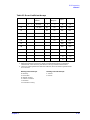
OUTP . . . . . . . . . . . . . . . . . . . . . . . . . . . . . . . . . . . . . . . . . . . . . . . . . . . . . . . . . . . . . . . . . . . 1-154
OUTP Reference Tables . . . . . . . . . . . . . . . . . . . . . . . . . . . . . . . . . . . . . . . . . . . . . . . . . . 1-160
P . . . . . . . . . . . . . . . . . . . . . . . . . . . . . . . . . . . . . . . . . . . . . . . . . . . . . . . . . . . . . . . . . . . . . . . 1-162
PARA . . . . . . . . . . . . . . . . . . . . . . . . . . . . . . . . . . . . . . . . . . . . . . . . . . . . . . . . . . . . . . . . . . . 1-163
Contents-viii
Contents
PARAL . . . . . . . . . . . . . . . . . . . . . . . . . . . . . . . . . . . . . . . . . . . . . . . . . . . . . . . . . . . . . . . . . .1-164
PAUS . . . . . . . . . . . . . . . . . . . . . . . . . . . . . . . . . . . . . . . . . . . . . . . . . . . . . . . . . . . . . . . . . . .1-165
PCB . . . . . . . . . . . . . . . . . . . . . . . . . . . . . . . . . . . . . . . . . . . . . . . . . . . . . . . . . . . . . . . . . . . .1-165
PCOL . . . . . . . . . . . . . . . . . . . . . . . . . . . . . . . . . . . . . . . . . . . . . . . . . . . . . . . . . . . . . . . . . . .1-166
PENN . . . . . . . . . . . . . . . . . . . . . . . . . . . . . . . . . . . . . . . . . . . . . . . . . . . . . . . . . . . . . . . . . . .1-167
PHAO . . . . . . . . . . . . . . . . . . . . . . . . . . . . . . . . . . . . . . . . . . . . . . . . . . . . . . . . . . . . . . . . . . .1-168
PHAS . . . . . . . . . . . . . . . . . . . . . . . . . . . . . . . . . . . . . . . . . . . . . . . . . . . . . . . . . . . . . . . . . . .1-168
PLOS . . . . . . . . . . . . . . . . . . . . . . . . . . . . . . . . . . . . . . . . . . . . . . . . . . . . . . . . . . . . . . . . . . .1-169
PLOT . . . . . . . . . . . . . . . . . . . . . . . . . . . . . . . . . . . . . . . . . . . . . . . . . . . . . . . . . . . . . . . . . . .1-169
PLT . . . . . . . . . . . . . . . . . . . . . . . . . . . . . . . . . . . . . . . . . . . . . . . . . . . . . . . . . . . . . . . . . . . . .1-170
PMTRTTIT . . . . . . . . . . . . . . . . . . . . . . . . . . . . . . . . . . . . . . . . . . . . . . . . . . . . . . . . . . . . . .1-171
POIN . . . . . . . . . . . . . . . . . . . . . . . . . . . . . . . . . . . . . . . . . . . . . . . . . . . . . . . . . . . . . . . . . . .1-172
POL . . . . . . . . . . . . . . . . . . . . . . . . . . . . . . . . . . . . . . . . . . . . . . . . . . . . . . . . . . . . . . . . . . . .1-173
PORE . . . . . . . . . . . . . . . . . . . . . . . . . . . . . . . . . . . . . . . . . . . . . . . . . . . . . . . . . . . . . . . . . . .1-174
PORT . . . . . . . . . . . . . . . . . . . . . . . . . . . . . . . . . . . . . . . . . . . . . . . . . . . . . . . . . . . . . . . . . . .1-175
PORTP . . . . . . . . . . . . . . . . . . . . . . . . . . . . . . . . . . . . . . . . . . . . . . . . . . . . . . . . . . . . . . . . . .1-176
POWE . . . . . . . . . . . . . . . . . . . . . . . . . . . . . . . . . . . . . . . . . . . . . . . . . . . . . . . . . . . . . . . . . . .1-177
POWL . . . . . . . . . . . . . . . . . . . . . . . . . . . . . . . . . . . . . . . . . . . . . . . . . . . . . . . . . . . . . . . . . . .1-178
POWM . . . . . . . . . . . . . . . . . . . . . . . . . . . . . . . . . . . . . . . . . . . . . . . . . . . . . . . . . . . . . . . . . .1-179
POWR . . . . . . . . . . . . . . . . . . . . . . . . . . . . . . . . . . . . . . . . . . . . . . . . . . . . . . . . . . . . . . . . . . .1-180
POWS . . . . . . . . . . . . . . . . . . . . . . . . . . . . . . . . . . . . . . . . . . . . . . . . . . . . . . . . . . . . . . . . . . .1-181
POWT . . . . . . . . . . . . . . . . . . . . . . . . . . . . . . . . . . . . . . . . . . . . . . . . . . . . . . . . . . . . . . . . . . .1-181
PRAN . . . . . . . . . . . . . . . . . . . . . . . . . . . . . . . . . . . . . . . . . . . . . . . . . . . . . . . . . . . . . . . . . . .1-182
PREP . . . . . . . . . . . . . . . . . . . . . . . . . . . . . . . . . . . . . . . . . . . . . . . . . . . . . . . . . . . . . . . . . . .1-182
PRES . . . . . . . . . . . . . . . . . . . . . . . . . . . . . . . . . . . . . . . . . . . . . . . . . . . . . . . . . . . . . . . . . . .1-183
PRI . . . . . . . . . . . . . . . . . . . . . . . . . . . . . . . . . . . . . . . . . . . . . . . . . . . . . . . . . . . . . . . . . . . . .1-184
PRIN . . . . . . . . . . . . . . . . . . . . . . . . . . . . . . . . . . . . . . . . . . . . . . . . . . . . . . . . . . . . . . . . . . . .1-185
PRINTALL . . . . . . . . . . . . . . . . . . . . . . . . . . . . . . . . . . . . . . . . . . . . . . . . . . . . . . . . . . . . . . .1-186
PRN . . . . . . . . . . . . . . . . . . . . . . . . . . . . . . . . . . . . . . . . . . . . . . . . . . . . . . . . . . . . . . . . . . . .1-187
PTOS . . . . . . . . . . . . . . . . . . . . . . . . . . . . . . . . . . . . . . . . . . . . . . . . . . . . . . . . . . . . . . . . . . .1-189
PURG . . . . . . . . . . . . . . . . . . . . . . . . . . . . . . . . . . . . . . . . . . . . . . . . . . . . . . . . . . . . . . . . . . .1-189
PWMC . . . . . . . . . . . . . . . . . . . . . . . . . . . . . . . . . . . . . . . . . . . . . . . . . . . . . . . . . . . . . . . . . .1-190
PWRLOSS . . . . . . . . . . . . . . . . . . . . . . . . . . . . . . . . . . . . . . . . . . . . . . . . . . . . . . . . . . . . . . .1-191
PWRMCAL . . . . . . . . . . . . . . . . . . . . . . . . . . . . . . . . . . . . . . . . . . . . . . . . . . . . . . . . . . . . . .1-191
PWRR . . . . . . . . . . . . . . . . . . . . . . . . . . . . . . . . . . . . . . . . . . . . . . . . . . . . . . . . . . . . . . . . . . .1-192
Q . . . . . . . . . . . . . . . . . . . . . . . . . . . . . . . . . . . . . . . . . . . . . . . . . . . . . . . . . . . . . . . . . . . . . . .1-192
RAI . . . . . . . . . . . . . . . . . . . . . . . . . . . . . . . . . . . . . . . . . . . . . . . . . . . . . . . . . . . . . . . . . . . . .1-193
RAWOFFS . . . . . . . . . . . . . . . . . . . . . . . . . . . . . . . . . . . . . . . . . . . . . . . . . . . . . . . . . . . . . . .1-194
READ . . . . . . . . . . . . . . . . . . . . . . . . . . . . . . . . . . . . . . . . . . . . . . . . . . . . . . . . . . . . . . . . . . .1-195
REAL . . . . . . . . . . . . . . . . . . . . . . . . . . . . . . . . . . . . . . . . . . . . . . . . . . . . . . . . . . . . . . . . . . .1-195
RECA . . . . . . . . . . . . . . . . . . . . . . . . . . . . . . . . . . . . . . . . . . . . . . . . . . . . . . . . . . . . . . . . . . .1-196
RECO . . . . . . . . . . . . . . . . . . . . . . . . . . . . . . . . . . . . . . . . . . . . . . . . . . . . . . . . . . . . . . . . . . .1-197
REF . . . . . . . . . . . . . . . . . . . . . . . . . . . . . . . . . . . . . . . . . . . . . . . . . . . . . . . . . . . . . . . . . . . .1-198
REF . . . . . . . . . . . . . . . . . . . . . . . . . . . . . . . . . . . . . . . . . . . . . . . . . . . . . . . . . . . . . . . . . . . .1-199
REFT . . . . . . . . . . . . . . . . . . . . . . . . . . . . . . . . . . . . . . . . . . . . . . . . . . . . . . . . . . . . . . . . . . .1-200
REIC . . . . . . . . . . . . . . . . . . . . . . . . . . . . . . . . . . . . . . . . . . . . . . . . . . . . . . . . . . . . . . . . . . . .1-200
RERCDONE . . . . . . . . . . . . . . . . . . . . . . . . . . . . . . . . . . . . . . . . . . . . . . . . . . . . . . . . . . . . . .1-201
RESC . . . . . . . . . . . . . . . . . . . . . . . . . . . . . . . . . . . . . . . . . . . . . . . . . . . . . . . . . . . . . . . . . . .1-201
RESD . . . . . . . . . . . . . . . . . . . . . . . . . . . . . . . . . . . . . . . . . . . . . . . . . . . . . . . . . . . . . . . . . . .1-202
Contents-ix
Contents
RESPDONE . . . . . . . . . . . . . . . . . . . . . . . . . . . . . . . . . . . . . . . . . . . . . . . . . . . . . . . . . . . . . 1-203
REST . . . . . . . . . . . . . . . . . . . . . . . . . . . . . . . . . . . . . . . . . . . . . . . . . . . . . . . . . . . . . . . . . . . 1-203
RETP . . . . . . . . . . . . . . . . . . . . . . . . . . . . . . . . . . . . . . . . . . . . . . . . . . . . . . . . . . . . . . . . . . . 1-204
REV . . . . . . . . . . . . . . . . . . . . . . . . . . . . . . . . . . . . . . . . . . . . . . . . . . . . . . . . . . . . . . . . . . . . 1-205
RF . . . . . . . . . . . . . . . . . . . . . . . . . . . . . . . . . . . . . . . . . . . . . . . . . . . . . . . . . . . . . . . . . . . . . 1-206
RFLP . . . . . . . . . . . . . . . . . . . . . . . . . . . . . . . . . . . . . . . . . . . . . . . . . . . . . . . . . . . . . . . . . . . 1-207
RIG . . . . . . . . . . . . . . . . . . . . . . . . . . . . . . . . . . . . . . . . . . . . . . . . . . . . . . . . . . . . . . . . . . . . 1-208
RLIMLINE . . . . . . . . . . . . . . . . . . . . . . . . . . . . . . . . . . . . . . . . . . . . . . . . . . . . . . . . . . . . . . 1-208
RLIMM . . . . . . . . . . . . . . . . . . . . . . . . . . . . . . . . . . . . . . . . . . . . . . . . . . . . . . . . . . . . . . . . . 1-209
RLIMSTP . . . . . . . . . . . . . . . . . . . . . . . . . . . . . . . . . . . . . . . . . . . . . . . . . . . . . . . . . . . . . . . 1-209
RLIMSTR . . . . . . . . . . . . . . . . . . . . . . . . . . . . . . . . . . . . . . . . . . . . . . . . . . . . . . . . . . . . . . . 1-210
RLIMTEST . . . . . . . . . . . . . . . . . . . . . . . . . . . . . . . . . . . . . . . . . . . . . . . . . . . . . . . . . . . . . . 1-210
RLIMVAL . . . . . . . . . . . . . . . . . . . . . . . . . . . . . . . . . . . . . . . . . . . . . . . . . . . . . . . . . . . . . . . 1-211
RSCO . . . . . . . . . . . . . . . . . . . . . . . . . . . . . . . . . . . . . . . . . . . . . . . . . . . . . . . . . . . . . . . . . . . 1-211
RST . . . . . . . . . . . . . . . . . . . . . . . . . . . . . . . . . . . . . . . . . . . . . . . . . . . . . . . . . . . . . . . . . . . . 1-212
S . . . . . . . . . . . . . . . . . . . . . . . . . . . . . . . . . . . . . . . . . . . . . . . . . . . . . . . . . . . . . . . . . . . . . . . 1-213
SADD . . . . . . . . . . . . . . . . . . . . . . . . . . . . . . . . . . . . . . . . . . . . . . . . . . . . . . . . . . . . . . . . . . . 1-214
SAMC . . . . . . . . . . . . . . . . . . . . . . . . . . . . . . . . . . . . . . . . . . . . . . . . . . . . . . . . . . . . . . . . . . 1-214
SAV . . . . . . . . . . . . . . . . . . . . . . . . . . . . . . . . . . . . . . . . . . . . . . . . . . . . . . . . . . . . . . . . . . . . 1-215
SAVECSV . . . . . . . . . . . . . . . . . . . . . . . . . . . . . . . . . . . . . . . . . . . . . . . . . . . . . . . . . . . . . . . 1-217
SAVEJPG . . . . . . . . . . . . . . . . . . . . . . . . . . . . . . . . . . . . . . . . . . . . . . . . . . . . . . . . . . . . . . . 1-217
SAVEUSEK . . . . . . . . . . . . . . . . . . . . . . . . . . . . . . . . . . . . . . . . . . . . . . . . . . . . . . . . . . . . . . 1-218
SAVU . . . . . . . . . . . . . . . . . . . . . . . . . . . . . . . . . . . . . . . . . . . . . . . . . . . . . . . . . . . . . . . . . . . 1-219
SCAL . . . . . . . . . . . . . . . . . . . . . . . . . . . . . . . . . . . . . . . . . . . . . . . . . . . . . . . . . . . . . . . . . . . 1-219
SCAP . . . . . . . . . . . . . . . . . . . . . . . . . . . . . . . . . . . . . . . . . . . . . . . . . . . . . . . . . . . . . . . . . . . 1-220
SDEL . . . . . . . . . . . . . . . . . . . . . . . . . . . . . . . . . . . . . . . . . . . . . . . . . . . . . . . . . . . . . . . . . . . 1-221
SDON . . . . . . . . . . . . . . . . . . . . . . . . . . . . . . . . . . . . . . . . . . . . . . . . . . . . . . . . . . . . . . . . . . 1-222
SEA . . . . . . . . . . . . . . . . . . . . . . . . . . . . . . . . . . . . . . . . . . . . . . . . . . . . . . . . . . . . . . . . . . . . 1-223
SEDI . . . . . . . . . . . . . . . . . . . . . . . . . . . . . . . . . . . . . . . . . . . . . . . . . . . . . . . . . . . . . . . . . . . 1-224
SEG . . . . . . . . . . . . . . . . . . . . . . . . . . . . . . . . . . . . . . . . . . . . . . . . . . . . . . . . . . . . . . . . . . . . 1-225
SEL . . . . . . . . . . . . . . . . . . . . . . . . . . . . . . . . . . . . . . . . . . . . . . . . . . . . . . . . . . . . . . . . . . . . 1-226
SELBND . . . . . . . . . . . . . . . . . . . . . . . . . . . . . . . . . . . . . . . . . . . . . . . . . . . . . . . . . . . . . . . . 1-227
SELL . . . . . . . . . . . . . . . . . . . . . . . . . . . . . . . . . . . . . . . . . . . . . . . . . . . . . . . . . . . . . . . . . . . 1-228
SEQ . . . . . . . . . . . . . . . . . . . . . . . . . . . . . . . . . . . . . . . . . . . . . . . . . . . . . . . . . . . . . . . . . . . . 1-229
SEQWAIT . . . . . . . . . . . . . . . . . . . . . . . . . . . . . . . . . . . . . . . . . . . . . . . . . . . . . . . . . . . . . . . 1-229
SET . . . . . . . . . . . . . . . . . . . . . . . . . . . . . . . . . . . . . . . . . . . . . . . . . . . . . . . . . . . . . . . . . . . . 1-230
SHOM . . . . . . . . . . . . . . . . . . . . . . . . . . . . . . . . . . . . . . . . . . . . . . . . . . . . . . . . . . . . . . . . . . 1-231
SING . . . . . . . . . . . . . . . . . . . . . . . . . . . . . . . . . . . . . . . . . . . . . . . . . . . . . . . . . . . . . . . . . . . 1-232
SLI . . . . . . . . . . . . . . . . . . . . . . . . . . . . . . . . . . . . . . . . . . . . . . . . . . . . . . . . . . . . . . . . . . . . . 1-233
SLOP . . . . . . . . . . . . . . . . . . . . . . . . . . . . . . . . . . . . . . . . . . . . . . . . . . . . . . . . . . . . . . . . . . . 1-234
SM8 . . . . . . . . . . . . . . . . . . . . . . . . . . . . . . . . . . . . . . . . . . . . . . . . . . . . . . . . . . . . . . . . . . . . 1-235
SMI . . . . . . . . . . . . . . . . . . . . . . . . . . . . . . . . . . . . . . . . . . . . . . . . . . . . . . . . . . . . . . . . . . . . 1-236
SMOO . . . . . . . . . . . . . . . . . . . . . . . . . . . . . . . . . . . . . . . . . . . . . . . . . . . . . . . . . . . . . . . . . . 1-237
SOFR . . . . . . . . . . . . . . . . . . . . . . . . . . . . . . . . . . . . . . . . . . . . . . . . . . . . . . . . . . . . . . . . . . . 1-237
SOFT . . . . . . . . . . . . . . . . . . . . . . . . . . . . . . . . . . . . . . . . . . . . . . . . . . . . . . . . . . . . . . . . . . . 1-238
SOUP . . . . . . . . . . . . . . . . . . . . . . . . . . . . . . . . . . . . . . . . . . . . . . . . . . . . . . . . . . . . . . . . . . . 1-238
SPAN . . . . . . . . . . . . . . . . . . . . . . . . . . . . . . . . . . . . . . . . . . . . . . . . . . . . . . . . . . . . . . . . . . . 1-239
SPEC . . . . . . . . . . . . . . . . . . . . . . . . . . . . . . . . . . . . . . . . . . . . . . . . . . . . . . . . . . . . . . . . . . . 1-240
SPEG . . . . . . . . . . . . . . . . . . . . . . . . . . . . . . . . . . . . . . . . . . . . . . . . . . . . . . . . . . . . . . . . . . . 1-243
Contents-x
Contents
SPLD . . . . . . . . . . . . . . . . . . . . . . . . . . . . . . . . . . . . . . . . . . . . . . . . . . . . . . . . . . . . . . . . . . .1-243
SPLID . . . . . . . . . . . . . . . . . . . . . . . . . . . . . . . . . . . . . . . . . . . . . . . . . . . . . . . . . . . . . . . . . . .1-244
SRE . . . . . . . . . . . . . . . . . . . . . . . . . . . . . . . . . . . . . . . . . . . . . . . . . . . . . . . . . . . . . . . . . . . .1-245
SSTAN . . . . . . . . . . . . . . . . . . . . . . . . . . . . . . . . . . . . . . . . . . . . . . . . . . . . . . . . . . . . . . . . . .1-246
STAR . . . . . . . . . . . . . . . . . . . . . . . . . . . . . . . . . . . . . . . . . . . . . . . . . . . . . . . . . . . . . . . . . . .1-247
STB? . . . . . . . . . . . . . . . . . . . . . . . . . . . . . . . . . . . . . . . . . . . . . . . . . . . . . . . . . . . . . . . . . . . .1-247
STDD . . . . . . . . . . . . . . . . . . . . . . . . . . . . . . . . . . . . . . . . . . . . . . . . . . . . . . . . . . . . . . . . . . .1-248
STDT . . . . . . . . . . . . . . . . . . . . . . . . . . . . . . . . . . . . . . . . . . . . . . . . . . . . . . . . . . . . . . . . . . .1-249
STEPSWP . . . . . . . . . . . . . . . . . . . . . . . . . . . . . . . . . . . . . . . . . . . . . . . . . . . . . . . . . . . . . . . .1-250
STOP . . . . . . . . . . . . . . . . . . . . . . . . . . . . . . . . . . . . . . . . . . . . . . . . . . . . . . . . . . . . . . . . . . .1-251
STOR . . . . . . . . . . . . . . . . . . . . . . . . . . . . . . . . . . . . . . . . . . . . . . . . . . . . . . . . . . . . . . . . . . .1-252
STORSEQ . . . . . . . . . . . . . . . . . . . . . . . . . . . . . . . . . . . . . . . . . . . . . . . . . . . . . . . . . . . . . . .1-253
STPSIZE . . . . . . . . . . . . . . . . . . . . . . . . . . . . . . . . . . . . . . . . . . . . . . . . . . . . . . . . . . . . . . . .1-253
SVCO . . . . . . . . . . . . . . . . . . . . . . . . . . . . . . . . . . . . . . . . . . . . . . . . . . . . . . . . . . . . . . . . . . .1-254
SWE . . . . . . . . . . . . . . . . . . . . . . . . . . . . . . . . . . . . . . . . . . . . . . . . . . . . . . . . . . . . . . . . . . . .1-255
SWPSTART . . . . . . . . . . . . . . . . . . . . . . . . . . . . . . . . . . . . . . . . . . . . . . . . . . . . . . . . . . . . . .1-256
SWR . . . . . . . . . . . . . . . . . . . . . . . . . . . . . . . . . . . . . . . . . . . . . . . . . . . . . . . . . . . . . . . . . . . .1-256
TAK . . . . . . . . . . . . . . . . . . . . . . . . . . . . . . . . . . . . . . . . . . . . . . . . . . . . . . . . . . . . . . . . . . . .1-257
TAKE4 . . . . . . . . . . . . . . . . . . . . . . . . . . . . . . . . . . . . . . . . . . . . . . . . . . . . . . . . . . . . . . . . . .1-258
TALKLIST . . . . . . . . . . . . . . . . . . . . . . . . . . . . . . . . . . . . . . . . . . . . . . . . . . . . . . . . . . . . . . .1-258
TERI . . . . . . . . . . . . . . . . . . . . . . . . . . . . . . . . . . . . . . . . . . . . . . . . . . . . . . . . . . . . . . . . . . . .1-259
TESS? . . . . . . . . . . . . . . . . . . . . . . . . . . . . . . . . . . . . . . . . . . . . . . . . . . . . . . . . . . . . . . . . . . .1-259
TIMDTRAN . . . . . . . . . . . . . . . . . . . . . . . . . . . . . . . . . . . . . . . . . . . . . . . . . . . . . . . . . . . . . .1-260
TIMESTAM . . . . . . . . . . . . . . . . . . . . . . . . . . . . . . . . . . . . . . . . . . . . . . . . . . . . . . . . . . . . . .1-260
STINT . . . . . . . . . . . . . . . . . . . . . . . . . . . . . . . . . . . . . . . . . . . . . . . . . . . . . . . . . . . . . . . . . .1-261
TIT . . . . . . . . . . . . . . . . . . . . . . . . . . . . . . . . . . . . . . . . . . . . . . . . . . . . . . . . . . . . . . . . . . . . .1-262
TITT . . . . . . . . . . . . . . . . . . . . . . . . . . . . . . . . . . . . . . . . . . . . . . . . . . . . . . . . . . . . . . . . . . . .1-263
TRA . . . . . . . . . . . . . . . . . . . . . . . . . . . . . . . . . . . . . . . . . . . . . . . . . . . . . . . . . . . . . . . . . . . .1-264
TRACK . . . . . . . . . . . . . . . . . . . . . . . . . . . . . . . . . . . . . . . . . . . . . . . . . . . . . . . . . . . . . . . . . .1-265
TRAP . . . . . . . . . . . . . . . . . . . . . . . . . . . . . . . . . . . . . . . . . . . . . . . . . . . . . . . . . . . . . . . . . . .1-265
TRL . . . . . . . . . . . . . . . . . . . . . . . . . . . . . . . . . . . . . . . . . . . . . . . . . . . . . . . . . . . . . . . . . . . . .1-266
TSSWI . . . . . . . . . . . . . . . . . . . . . . . . . . . . . . . . . . . . . . . . . . . . . . . . . . . . . . . . . . . . . . . . . .1-267
TST? . . . . . . . . . . . . . . . . . . . . . . . . . . . . . . . . . . . . . . . . . . . . . . . . . . . . . . . . . . . . . . . . . . . .1-267
TSTIO . . . . . . . . . . . . . . . . . . . . . . . . . . . . . . . . . . . . . . . . . . . . . . . . . . . . . . . . . . . . . . . . . . .1-268
TSTP . . . . . . . . . . . . . . . . . . . . . . . . . . . . . . . . . . . . . . . . . . . . . . . . . . . . . . . . . . . . . . . . . . .1-269
TTL . . . . . . . . . . . . . . . . . . . . . . . . . . . . . . . . . . . . . . . . . . . . . . . . . . . . . . . . . . . . . . . . . . . . .1-270
UCONV . . . . . . . . . . . . . . . . . . . . . . . . . . . . . . . . . . . . . . . . . . . . . . . . . . . . . . . . . . . . . . . . .1-271
UP . . . . . . . . . . . . . . . . . . . . . . . . . . . . . . . . . . . . . . . . . . . . . . . . . . . . . . . . . . . . . . . . . . . . . .1-271
USEPASC . . . . . . . . . . . . . . . . . . . . . . . . . . . . . . . . . . . . . . . . . . . . . . . . . . . . . . . . . . . . . . .1-272
USESENS . . . . . . . . . . . . . . . . . . . . . . . . . . . . . . . . . . . . . . . . . . . . . . . . . . . . . . . . . . . . . . .1-272
VELOFACT . . . . . . . . . . . . . . . . . . . . . . . . . . . . . . . . . . . . . . . . . . . . . . . . . . . . . . . . . . . . . .1-273
VIEM . . . . . . . . . . . . . . . . . . . . . . . . . . . . . . . . . . . . . . . . . . . . . . . . . . . . . . . . . . . . . . . . . . .1-273
VOFF . . . . . . . . . . . . . . . . . . . . . . . . . . . . . . . . . . . . . . . . . . . . . . . . . . . . . . . . . . . . . . . . . . .1-274
WAIT . . . . . . . . . . . . . . . . . . . . . . . . . . . . . . . . . . . . . . . . . . . . . . . . . . . . . . . . . . . . . . . . . . .1-274
WAVD . . . . . . . . . . . . . . . . . . . . . . . . . . . . . . . . . . . . . . . . . . . . . . . . . . . . . . . . . . . . . . . . . . .1-275
WAVE . . . . . . . . . . . . . . . . . . . . . . . . . . . . . . . . . . . . . . . . . . . . . . . . . . . . . . . . . . . . . . . . . . .1-275
WID . . . . . . . . . . . . . . . . . . . . . . . . . . . . . . . . . . . . . . . . . . . . . . . . . . . . . . . . . . . . . . . . . . . .1-276
WIND . . . . . . . . . . . . . . . . . . . . . . . . . . . . . . . . . . . . . . . . . . . . . . . . . . . . . . . . . . . . . . . . . . .1-277
WRSK . . . . . . . . . . . . . . . . . . . . . . . . . . . . . . . . . . . . . . . . . . . . . . . . . . . . . . . . . . . . . . . . . . .1-278
Contents-xi
Contents
2. Introduction to Instrument Control
Using This Chapter . . . . . . . . . . . . . . . . . . . . . . . . . . . . . . . . . . . . . . . . . . . . . . . . . . . . . . . . . . 2-2
Instrument Control using the VXIplug&play Driver . . . . . . . . . . . . . . . . . . . . . . . . . . . . . . . 2-3
Requirements . . . . . . . . . . . . . . . . . . . . . . . . . . . . . . . . . . . . . . . . . . . . . . . . . . . . . . . . . . . . . 2-3
Installing the VXIplug&play Driver . . . . . . . . . . . . . . . . . . . . . . . . . . . . . . . . . . . . . . . . . . . 2-3
System Setup . . . . . . . . . . . . . . . . . . . . . . . . . . . . . . . . . . . . . . . . . . . . . . . . . . . . . . . . . . . . . 2-4
Verifying the Bus Connection . . . . . . . . . . . . . . . . . . . . . . . . . . . . . . . . . . . . . . . . . . . . . . . . 2-5
Controlling the Analyzer with the VXIplug&play Driver . . . . . . . . . . . . . . . . . . . . . . . . . . 2-7
Instrument Control using HP BASIC. . . . . . . . . . . . . . . . . . . . . . . . . . . . . . . . . . . . . . . . . . . . 2-9
Required Equipment . . . . . . . . . . . . . . . . . . . . . . . . . . . . . . . . . . . . . . . . . . . . . . . . . . . . . . . 2-9
System Setup and GPIB Verification . . . . . . . . . . . . . . . . . . . . . . . . . . . . . . . . . . . . . . . . . 2-10
Sending Commands . . . . . . . . . . . . . . . . . . . . . . . . . . . . . . . . . . . . . . . . . . . . . . . . . . . . . . . 2-12
3. GPIB Programming
Analyzer Command Syntax . . . . . . . . . . . . . . . . . . . . . . . . . . . . . . . . . . . . . . . . . . . . . . . . . . . 3-2
Code Naming Convention . . . . . . . . . . . . . . . . . . . . . . . . . . . . . . . . . . . . . . . . . . . . . . . . . . . 3-2
Valid Characters . . . . . . . . . . . . . . . . . . . . . . . . . . . . . . . . . . . . . . . . . . . . . . . . . . . . . . . . . . 3-3
Units . . . . . . . . . . . . . . . . . . . . . . . . . . . . . . . . . . . . . . . . . . . . . . . . . . . . . . . . . . . . . . . . . . . . 3-4
Command Formats . . . . . . . . . . . . . . . . . . . . . . . . . . . . . . . . . . . . . . . . . . . . . . . . . . . . . . . . 3-4
Analyzer Operation . . . . . . . . . . . . . . . . . . . . . . . . . . . . . . . . . . . . . . . . . . . . . . . . . . . . . . . . . . 3-6
Held Commands . . . . . . . . . . . . . . . . . . . . . . . . . . . . . . . . . . . . . . . . . . . . . . . . . . . . . . . . . . . 3-6
Operation Complete . . . . . . . . . . . . . . . . . . . . . . . . . . . . . . . . . . . . . . . . . . . . . . . . . . . . . . . . 3-6
GPIB Operation . . . . . . . . . . . . . . . . . . . . . . . . . . . . . . . . . . . . . . . . . . . . . . . . . . . . . . . . . . . . . 3-7
Device Types . . . . . . . . . . . . . . . . . . . . . . . . . . . . . . . . . . . . . . . . . . . . . . . . . . . . . . . . . . . . . . 3-7
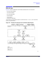
GPIB Bus Structure . . . . . . . . . . . . . . . . . . . . . . . . . . . . . . . . . . . . . . . . . . . . . . . . . . . . . . . 3-8
GPIB Requirements . . . . . . . . . . . . . . . . . . . . . . . . . . . . . . . . . . . . . . . . . . . . . . . . . . . . . . 3-10
GPIB Operational Capabilities . . . . . . . . . . . . . . . . . . . . . . . . . . . . . . . . . . . . . . . . . . . . . . 3-11
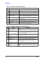
Bus Device Modes . . . . . . . . . . . . . . . . . . . . . . . . . . . . . . . . . . . . . . . . . . . . . . . . . . . . . . . . 3-12
Setting GPIB Addresses . . . . . . . . . . . . . . . . . . . . . . . . . . . . . . . . . . . . . . . . . . . . . . . . . . . 3-14
Response to GPIB Meta-Messages (IEEE-488 Universal Commands) . . . . . . . . . . . . . . 3-14
IEEE 488.2 Common Commands . . . . . . . . . . . . . . . . . . . . . . . . . . . . . . . . . . . . . . . . . . . . 3-16
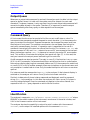
Calibration . . . . . . . . . . . . . . . . . . . . . . . . . . . . . . . . . . . . . . . . . . . . . . . . . . . . . . . . . . . . . . . 3-17
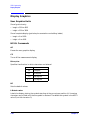
Display Graphics . . . . . . . . . . . . . . . . . . . . . . . . . . . . . . . . . . . . . . . . . . . . . . . . . . . . . . . . . . 3-20
User Graphics Units . . . . . . . . . . . . . . . . . . . . . . . . . . . . . . . . . . . . . . . . . . . . . . . . . . . . . . 3-20
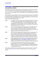
HP-GL Commands . . . . . . . . . . . . . . . . . . . . . . . . . . . . . . . . . . . . . . . . . . . . . . . . . . . . . . . 3-20
Disk File Names . . . . . . . . . . . . . . . . . . . . . . . . . . . . . . . . . . . . . . . . . . . . . . . . . . . . . . . . . . . 3-23
4. Reading Analyzer Data
Output Queue . . . . . . . . . . . . . . . . . . . . . . . . . . . . . . . . . . . . . . . . . . . . . . . . . . . . . . . . . . . . . . 4-2
Command Query . . . . . . . . . . . . . . . . . . . . . . . . . . . . . . . . . . . . . . . . . . . . . . . . . . . . . . . . . . . . 4-2
Identification . . . . . . . . . . . . . . . . . . . . . . . . . . . . . . . . . . . . . . . . . . . . . . . . . . . . . . . . . . . . . . . 4-2
Output Syntax . . . . . . . . . . . . . . . . . . . . . . . . . . . . . . . . . . . . . . . . . . . . . . . . . . . . . . . . . . . . . 4-3
Marker Data . . . . . . . . . . . . . . . . . . . . . . . . . . . . . . . . . . . . . . . . . . . . . . . . . . . . . . . . . . . . . . . 4-4
Array-Data Formats . . . . . . . . . . . . . . . . . . . . . . . . . . . . . . . . . . . . . . . . . . . . . . . . . . . . . . . . . 4-6
Trace-Data Transfers . . . . . . . . . . . . . . . . . . . . . . . . . . . . . . . . . . . . . . . . . . . . . . . . . . . . . . . . 4-8
Stimulus-Related Values . . . . . . . . . . . . . . . . . . . . . . . . . . . . . . . . . . . . . . . . . . . . . . . . . . . . . 4-9
Contents-xii
Contents
5. Data Processing Chain
Using This Chapter . . . . . . . . . . . . . . . . . . . . . . . . . . . . . . . . . . . . . . . . . . . . . . . . . . . . . . . . . .5-2
Data Arrays . . . . . . . . . . . . . . . . . . . . . . . . . . . . . . . . . . . . . . . . . . . . . . . . . . . . . . . . . . . . . . . .5-3
Common Output Commands . . . . . . . . . . . . . . . . . . . . . . . . . . . . . . . . . . . . . . . . . . . . . . . . . . .5-4
Fast Data Transfer Commands . . . . . . . . . . . . . . . . . . . . . . . . . . . . . . . . . . . . . . . . . . . . . . . .5-5
Data Levels . . . . . . . . . . . . . . . . . . . . . . . . . . . . . . . . . . . . . . . . . . . . . . . . . . . . . . . . . . . . . . . .5-6
Pre-Raw Data . . . . . . . . . . . . . . . . . . . . . . . . . . . . . . . . . . . . . . . . . . . . . . . . . . . . . . . . . . . . .5-6
Raw Data . . . . . . . . . . . . . . . . . . . . . . . . . . . . . . . . . . . . . . . . . . . . . . . . . . . . . . . . . . . . . . . . .5-6
Error Coefficients . . . . . . . . . . . . . . . . . . . . . . . . . . . . . . . . . . . . . . . . . . . . . . . . . . . . . . . . . .5-6
Error-Corrected Data . . . . . . . . . . . . . . . . . . . . . . . . . . . . . . . . . . . . . . . . . . . . . . . . . . . . . . .5-6
Formatted Data . . . . . . . . . . . . . . . . . . . . . . . . . . . . . . . . . . . . . . . . . . . . . . . . . . . . . . . . . . . .5-7
Learn String and Calibration-Kit String . . . . . . . . . . . . . . . . . . . . . . . . . . . . . . . . . . . . . . . . .5-7
6. Error Reporting
Using This Chapter . . . . . . . . . . . . . . . . . . . . . . . . . . . . . . . . . . . . . . . . . . . . . . . . . . . . . . . . . .6-2
Status Reporting . . . . . . . . . . . . . . . . . . . . . . . . . . . . . . . . . . . . . . . . . . . . . . . . . . . . . . . . . . . .6-3
The Status Byte . . . . . . . . . . . . . . . . . . . . . . . . . . . . . . . . . . . . . . . . . . . . . . . . . . . . . . . . . . . . .6-6
The Event-Status Register and Event-Status Register B . . . . . . . . . . . . . . . . . . . . . . . . . . . .6-7
Error Output . . . . . . . . . . . . . . . . . . . . . . . . . . . . . . . . . . . . . . . . . . . . . . . . . . . . . . . . . . . . . . .6-8
Error Messages in Numerical Order . . . . . . . . . . . . . . . . . . . . . . . . . . . . . . . . . . . . . . . . . . . .6-9
7. Programming Examples
Using This Chapter . . . . . . . . . . . . . . . . . . . . . . . . . . . . . . . . . . . . . . . . . . . . . . . . . . . . . . . . . .7-2
Measurement Process . . . . . . . . . . . . . . . . . . . . . . . . . . . . . . . . . . . . . . . . . . . . . . . . . . . . . . . .7-3
Step 1. Setting Up the Instrument . . . . . . . . . . . . . . . . . . . . . . . . . . . . . . . . . . . . . . . . . . . .7-3
Step 2. Calibrating the Test Setup . . . . . . . . . . . . . . . . . . . . . . . . . . . . . . . . . . . . . . . . . . . .7-3
Step 3. Connecting the Device under Test . . . . . . . . . . . . . . . . . . . . . . . . . . . . . . . . . . . . . .7-4
Step 4. Taking the Measurement Data . . . . . . . . . . . . . . . . . . . . . . . . . . . . . . . . . . . . . . . . .7-4
Step 5. Post-Processing the Measurement Data . . . . . . . . . . . . . . . . . . . . . . . . . . . . . . . . .7-4
Step 6. Transferring the Measurement Data . . . . . . . . . . . . . . . . . . . . . . . . . . . . . . . . . . . .7-4
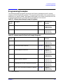
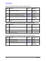
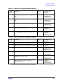
Programming Examples . . . . . . . . . . . . . . . . . . . . . . . . . . . . . . . . . . . . . . . . . . . . . . . . . . . . . .7-5
Program Information . . . . . . . . . . . . . . . . . . . . . . . . . . . . . . . . . . . . . . . . . . . . . . . . . . . . . . .7-8
Analyzer Features Helpful in Developing Programming Routines . . . . . . . . . . . . . . . . . . .7-8
Measurement Setup Examples . . . . . . . . . . . . . . . . . . . . . . . . . . . . . . . . . . . . . . . . . . . . . . . .7-10
Example 1A: Setting Parameters . . . . . . . . . . . . . . . . . . . . . . . . . . . . . . . . . . . . . . . . . . . .7-10
Example 1B: Verifying Parameters . . . . . . . . . . . . . . . . . . . . . . . . . . . . . . . . . . . . . . . . . . .7-21
Measurement Calibration Examples . . . . . . . . . . . . . . . . . . . . . . . . . . . . . . . . . . . . . . . . . . .7-23
Calibration Kits . . . . . . . . . . . . . . . . . . . . . . . . . . . . . . . . . . . . . . . . . . . . . . . . . . . . . . . . . .7-24
Example 2A: Response Calibration . . . . . . . . . . . . . . . . . . . . . . . . . . . . . . . . . . . . . . . . . . .7-24
Example 2B: 1-Port Calibration . . . . . . . . . . . . . . . . . . . . . . . . . . . . . . . . . . . . . . . . . . . . .7-26
Example 2C: Enhanced Response Calibration . . . . . . . . . . . . . . . . . . . . . . . . . . . . . . . . . .7-30
Example 2D: Full 2-Port Measurement Calibration . . . . . . . . . . . . . . . . . . . . . . . . . . . . .7-33
Example 2E: Adapter Removal Calibration . . . . . . . . . . . . . . . . . . . . . . . . . . . . . . . . . . . .7-38
Example 2F: Using Raw Data to Create a Calibration (Simmcal) . . . . . . . . . . . . . . . . . .7-41
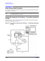
Example 2G: Take4 — Error Correction Processed on an External PC . . . . . . . . . . . . . .7-48
Measurement Data Transfer Examples . . . . . . . . . . . . . . . . . . . . . . . . . . . . . . . . . . . . . . . . .7-56
Trace-Data Formats and Transfers . . . . . . . . . . . . . . . . . . . . . . . . . . . . . . . . . . . . . . . . . . .7-56
Example 3A: Data Transfer Using Markers . . . . . . . . . . . . . . . . . . . . . . . . . . . . . . . . . . . .7-57
Contents-xiii
Contents
Example 3B: Data Transfer Using FORM 4 (ASCII Transfer) . . . . . . . . . . . . . . . . . . . . . 7-59
Example 3C: Data Transfer Using Floating-Point Numbers . . . . . . . . . . . . . . . . . . . . . . 7-62
Example 3D: Data Transfer Using Frequency-Array Information . . . . . . . . . . . . . . . . . . 7-64
Example 3E: Data Transfer Using FORM 1 (Internal-Binary Format) . . . . . . . . . . . . . . 7-67
Measurement Process Synchronization Examples . . . . . . . . . . . . . . . . . . . . . . . . . . . . . . . . 7-69
Status Reporting . . . . . . . . . . . . . . . . . . . . . . . . . . . . . . . . . . . . . . . . . . . . . . . . . . . . . . . . . 7-69
Example 4A: Using the Error Queue . . . . . . . . . . . . . . . . . . . . . . . . . . . . . . . . . . . . . . . . . 7-70
Example 4B: Generating Interrupts . . . . . . . . . . . . . . . . . . . . . . . . . . . . . . . . . . . . . . . . . 7-72
Example 4C: Power Meter Calibration . . . . . . . . . . . . . . . . . . . . . . . . . . . . . . . . . . . . . . . 7-75
Analyzer System Setup Examples . . . . . . . . . . . . . . . . . . . . . . . . . . . . . . . . . . . . . . . . . . . . . 7-79
Saving and Recalling Instrument States . . . . . . . . . . . . . . . . . . . . . . . . . . . . . . . . . . . . . . 7-79
Example 5A: Using the Learn String . . . . . . . . . . . . . . . . . . . . . . . . . . . . . . . . . . . . . . . . . 7-79
Example 5B: Reading Calibration Data . . . . . . . . . . . . . . . . . . . . . . . . . . . . . . . . . . . . . . . 7-81
Example 5C: Saving and Restoring the Analyzer Instrument State . . . . . . . . . . . . . . . . 7-84
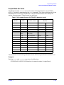
List-Frequency and Limit-Test Table Examples . . . . . . . . . . . . . . . . . . . . . . . . . . . . . . . . . . 7-87
Using List Frequency Sweep Mode . . . . . . . . . . . . . . . . . . . . . . . . . . . . . . . . . . . . . . . . . . 7-87
Example 6A: Setting Up a List Frequency Table in Stepped List Mode . . . . . . . . . . . . . 7-88
Example 6B: Setting Up a List Frequency Table in Swept List Mode . . . . . . . . . . . . . . . 7-90
Example 6C: Selecting a Single Segment from a Table of Segments . . . . . . . . . . . . . . . . 7-94
Using Limit Lines to Perform PASS/FAIL Tests . . . . . . . . . . . . . . . . . . . . . . . . . . . . . . . . 7-96
Example 6D: Setting Up a Limit-Test Table . . . . . . . . . . . . . . . . . . . . . . . . . . . . . . . . . . . 7-96
Example 6E: Performing PASS/FAIL Tests While Tuning . . . . . . . . . . . . . . . . . . . . . . . . 7-99
Report Generation Examples . . . . . . . . . . . . . . . . . . . . . . . . . . . . . . . . . . . . . . . . . . . . . . . . 7-102
Example 7A: Operation Using Talker/Listener Mode . . . . . . . . . . . . . . . . . . . . . . . . . . . 7-102
Example 7B: Controlling Peripherals Using Pass-Control Mode . . . . . . . . . . . . . . . . . . 7-104
Example 7C: Printing with the Parallel Port . . . . . . . . . . . . . . . . . . . . . . . . . . . . . . . . . . 7-107
Example 7D: Plotting to a File and Transferring the File Data to a Plotter . . . . . . . . . 7-109
Example 7E: Reading Plot Files from a Disk . . . . . . . . . . . . . . . . . . . . . . . . . . . . . . . . . . 7-111
Example 7F: Reading ASCII Disk Files to the Instrument Controller’s Disk File . . . . 7-118
Mixer Measurement Example. . . . . . . . . . . . . . . . . . . . . . . . . . . . . . . . . . . . . . . . . . . . . . . . 7-122
Example 8A: Comparison of Two Mixers — Group Delay, Amplitude or Phase . . . . . . 7-122
Limit Line and Data Point Special Functions . . . . . . . . . . . . . . . . . . . . . . . . . . . . . . . . . . . 7-126
Overview . . . . . . . . . . . . . . . . . . . . . . . . . . . . . . . . . . . . . . . . . . . . . . . . . . . . . . . . . . . . . . 7-126
Constants Used Throughout This Document . . . . . . . . . . . . . . . . . . . . . . . . . . . . . . . . . 7-131
Output Limit Test Pass/Fail Status Per Limit Segment . . . . . . . . . . . . . . . . . . . . . . . . . 7-131
Output Pass/Fail Status for All Segments . . . . . . . . . . . . . . . . . . . . . . . . . . . . . . . . . . . . 7-132
Output Minimum and Maximum Point Per Limit Segment . . . . . . . . . . . . . . . . . . . . . . 7-133
Output Minimum and Maximum Point for All Segments . . . . . . . . . . . . . . . . . . . . . . . . 7-134
Output Data Per Point . . . . . . . . . . . . . . . . . . . . . . . . . . . . . . . . . . . . . . . . . . . . . . . . . . . 7-137
Output Data Per Range of Points . . . . . . . . . . . . . . . . . . . . . . . . . . . . . . . . . . . . . . . . . . . 7-138
Output Limit Pass/Fail by Channel . . . . . . . . . . . . . . . . . . . . . . . . . . . . . . . . . . . . . . . . . 7-138
A. Preset Conditions
Preset State . . . . . . . . . . . . . . . . . . . . . . . . . . . . . . . . . . . . . . . . . . . . . . . . . . . . . . . . . . . . . . . .A-2
B. Command Listings
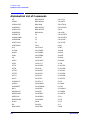
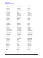
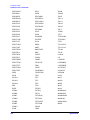
Alphabetical List of Commands . . . . . . . . . . . . . . . . . . . . . . . . . . . . . . . . . . . . . . . . . . . . . . . .B-2
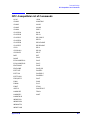
OPC-Compatible List of Commands. . . . . . . . . . . . . . . . . . . . . . . . . . . . . . . . . . . . . . . . . . . . .B-9
Contents-xiv
1 Alphabetical Command Reference
1-1
Alphabetical Command Reference
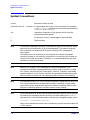
Symbol Conventions
Symbol Conventions
<num>
Required numerical data.
<choice1|choice2|…|choicen> An appendage that is part of the command. For example,
FORMAT<DOS|LIF> indicates that the actual commands are
FORMATDOS and FORMATLIF.
<$>
Indicates a character string operand which must be
enclosed by double quotes.
|
An either/or choice in appendages or optional data.
[]
Optional data.
NOTE
A terminator indicates the end of a command string, and this manual uses a
semicolon as the terminator in all syntax examples. The network analyzer
also interprets line feeds and GPIB end or identify (EOI) messages as
terminators.
Terminators are not necessary for the analyzer to interpret commands
correctly, however in the case of a syntax error, the analyzer will attempt to
recover at the next terminator. Therefore, it is recommended that you each
command include a terminator.
NOTE
Because this chapter is an “Alphabetical Command Reference,” the
commands have been listed alphabetically, rather than by function, in both
the “Syntax” sections and the “Description” sections. Therefore, commands
grouped together in the “Syntax” sections, are grouped alphabetically and/or
due to common syntax form, not necessarily due to common functionality.
NOTE
The softkeys listed in the “Front Panel Equivalents” tables may not be in the
first menu viewed when the associated hardkey is pressed. In many cases,
more than one key press will be required to locate the softkey. Refer to your
analyzer’s reference guide for the exact location of any softkey.
NOTE
Some commands that do not have an associated query syntax can be queried
by sending the command (without a value) and then sending the OUTPACTI
command, as in the following example that queries the segment power value:
10 OUTPUT 716;”SEGPOWER;OUTPACTI;”
Many of the commands that do have a listed query syntax can also be queried
in this manner.
1-2
Chapter 1
Alphabetical Command Reference
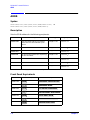
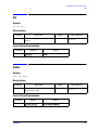
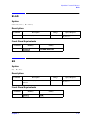
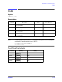
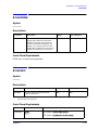
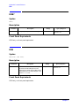
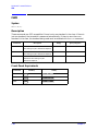
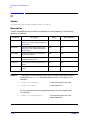
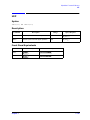
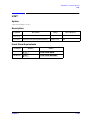
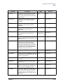
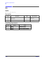
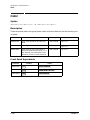
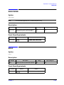
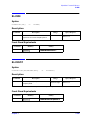
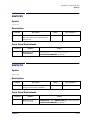
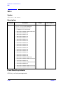
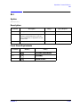
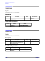
AB
AB
Syntax
AB; or AB?;
Description
Command
AB
Description
Range
Measures and displays A/B on the active
channel.
N/A
Query Response
<0|1><LF>
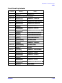
Front Panel Equivalents
Command
Hardkey
AB
Softkey
A/B
Meas
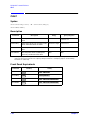
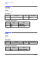
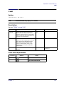
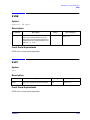
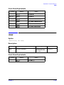
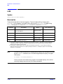
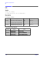
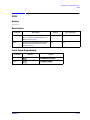
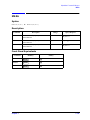
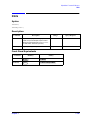
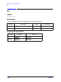
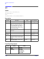
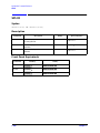
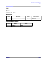
ADAP1
Syntax
ADAP1<num>[S]; or ADAP1?;
NOTE
This command only applies to ES model analyzers.
Description
Command
ADAP1
Description
Sets adapter electrical delay.
Range
±10 seconds
Query Response
<num><LF>
Front Panel Equivalents
Command
ADAP1
Chapter 1
Hardkey
Cal
Softkey
ADAPTER DELAY
1-3
Alphabetical Command Reference
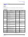
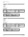
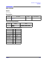
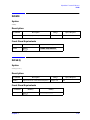
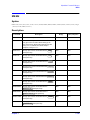
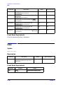
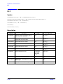
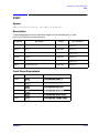
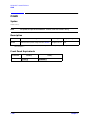
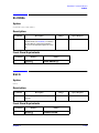
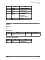
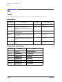
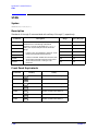
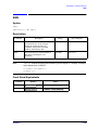
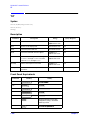
ADDR
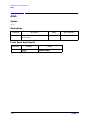
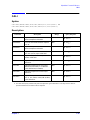
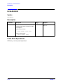
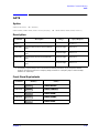
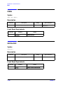
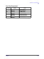
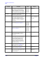
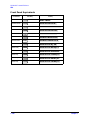
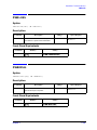
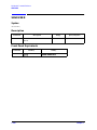
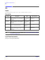
ADDR
Syntax
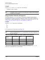
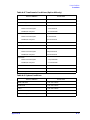
ADDR<CONT|DISC|LSRC|PERI|PLOT|POWM|PRIN><num>; or
ADDR<CONT|DISC|LSRC|PERI|PLOT|POWM|PRIN>?;
Description
Sets the GPIB address for the following peripherals.
Command
Description
Range
Query Response
ADDRCONT
Controller GPIB address. The address
where control is returned after a pass
control.
integers 0–30
<num><LF>
ADDRDISC
External disk drive GPIB address.
integers 0–30
<num><LF>
ADDRLSRC1
LO source GPIB address.
integers 0–30
<num><LF>
ADDRPERI
Peripheral GPIB address (for sequencing).
See also TITTPERI.
integers 0–30
<num><LF>
ADDRPLOT
Plotter GPIB address.
integers 0–30
<num><LF>
ADDRPOWM
Power meter GPIB address.
integers 0–30
<num><LF>
ADDRPRIN
Printer GPIB address.
integers 0–30
<num><LF>
1. This command only applies to 8753ET/ES analyzers.
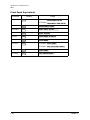
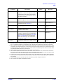
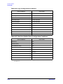
Front Panel Equivalents
Command
Hardkey
Softkey
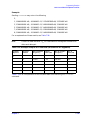
ADDRCONT
Local
ADDRESS: CONTROLLER
ADDRDISC
Local
ADDRESS: DISK
ADDRLSRC
Local
LO SOURCE ADDRESS
ADDRPERI
Seq
PERIPHERAL GPIB ADDR
ADDRPLOT
Local
PLTR PORT GPIB
ADDRPOWM
Local
ADDRESS: P MTR/GPIB
ADDRPRIN
Local
PRNTR PORT GPIB
1-4
Chapter 1
Alphabetical Command Reference
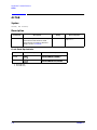
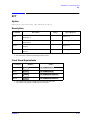
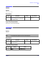
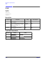
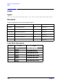
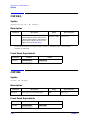
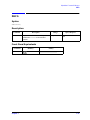
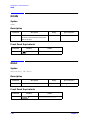
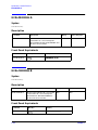
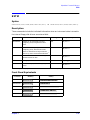
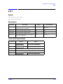
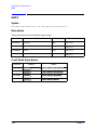
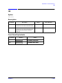
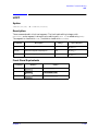
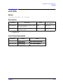
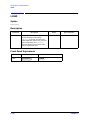
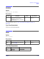
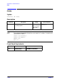
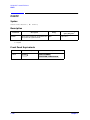
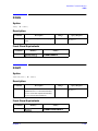
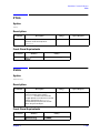
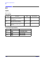
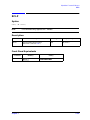
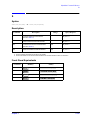
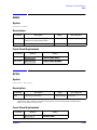
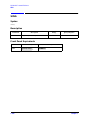
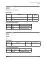
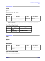
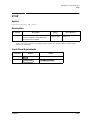
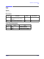
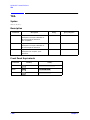
ADPT
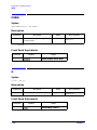
ADPT
Syntax
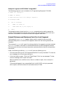
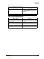
ADPT<COAX|WAVE>; or ADPT<COAX|WAVE>?;
Description
Command
Description
Range
Query Response
ADPTCOAX
Sets adapter to coaxial.
N/A
<0|1><LF>
ADPTWAVE
Sets adapter to waveguide.
N/A
<0|1><LF>
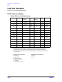
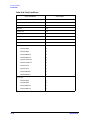
Front Panel Equivalents
Command
Hardkey
Softkey
ADPTCOAX
Cal
ADAPTER COAX
ADPTWAVE
Cal
ADAPTER WAVEGUIDE
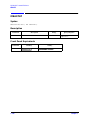
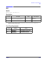
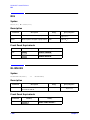
ALC
Syntax
ALC<ON|OFF>; or ALC?;
Description
Command
ALC
Description
Range
ALC control. For service use only.
N/A
Query Response
<0|1><LF>
Front Panel Equivalents
Command
ALC
Chapter 1
Hardkey
System
Softkey
ALC ON OFF
1-5
Alphabetical Command Reference
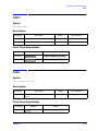
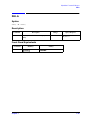
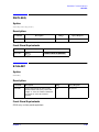
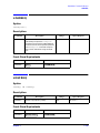
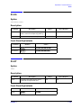
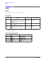
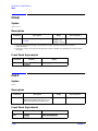
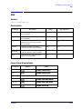
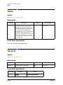
ALTAB
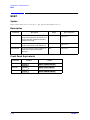
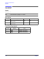
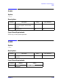
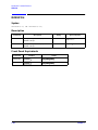
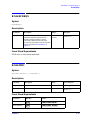
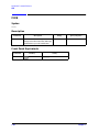
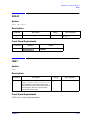
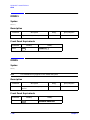
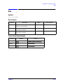
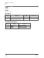
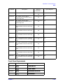
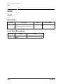
ALTAB
Syntax
ALTAB; or ALTAB?;
Description
Command
ALTAB
Description
Range
Places the analyzer in the alternate inputs
measurement mode, where A and B
measurements are made on alternate
sweeps. See also “CHOPAB.”
N/A
Query Response
<0|1><LF>
Front Panel Equivalents
Command
Hardkey
Softkey
ALTAB
Cal
ALTERNATE A and B 1
ALTAB
Cal
ALTERNATE RFL/TRAN 2
1. ES models only.
2. ET models only.
1-6
Chapter 1
Alphabetical Command Reference
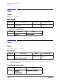
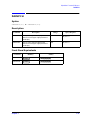
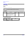
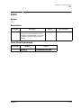
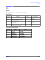
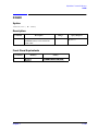
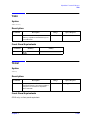
ANAB
ANAB
Syntax
ANAB<ON|OFF>; or ANAB?;
Description
Command
ANAB
Description
Range
Enables and disables the analog bus for
service use.
N/A
Query Response
<0|1><LF>
Front Panel Equivalents
Command
ANAB
Chapter 1
Hardkey
System
Softkey
ANALOG BUS ON OFF
1-7
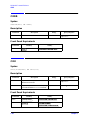
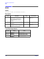
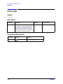
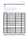
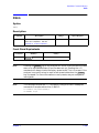
Alphabetical Command Reference
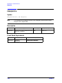
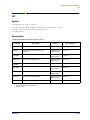
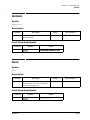
ANAI
ANAI
Syntax
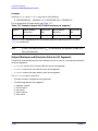
ANAI<num>; or ANAI?;
ANAI; or ANAI?;
Description
Command
Description
Range
Query Response
ANAI1
Measures and displays the data at the
auxiliary input (ANALOG IN).
integers 1–31
<0|1><LF>
ANAI2
Measures and displays the data at the
auxiliary input (ANALOG IN).
N/A
<0|1><LF>
1. When the analog bus is enabled (ANABON), this command requires that the complementary information (<num>)
be sent.
2. When the analog bus is disabled (ANABOFF), this command does not require the <num> parameter.
Front Panel Equivalents
Command
ANAI
1-8
Hardkey
Meas
Softkey
ANALOG IN Aux Input
Chapter 1
Alphabetical Command Reference
AR
AR
Syntax
AR; or AR?;
Description
Command
AR
Description
Range
Measures and displays A/R on the active
channel.
N/A
Query Response
<0|1><LF>
Front Panel Equivalents
Command
Hardkey
AR
Softkey
A/R
Meas
ASEG
Syntax
ASEG; or ASEG?;
Description
Command
ASEG
Description
Range
Uses all segments for list frequency
sweep. See also “SSEG.”
N/A
Query Response
<0|1><LF>
Front Panel Equivalents
Command
ASEG
Chapter 1
Hardkey
Sweep Setup
Softkey
ALL SEGS SWEEP
1-9
Alphabetical Command Reference
ASSS
ASSS
Syntax
ASSS;
Description
Command
ASSS
Description
Range
Asserts the sequence status bit to in-turn
generate SRQ.
N/A
Query Response
N/A
Front Panel Equivalents
Command
ASSS
1-10
Hardkey
Seq
Softkey
ASSERT SRQ
Chapter 1
Alphabetical Command Reference
ATT
ATT
Syntax
ATT<A|B|P1|P2><num>[DB]; or ATT<A|B|P1|P2>?;
Description
Command
Description
Range
Query Response
ATTA 1
Selects the amount of attenuation at
attenuator A.
0–55 dB
<num><LF>
ATTB1
Selects the amount of attenuation at
attenuator B.
0–55 dB
<num><LF>
ATTP12
Selects the amount of attenuation at
PORT 1.
0–70 dB
<num><LF>
ATTP22
Selects the amount of attenuation at
PORT 2.
0–70 dB
<num><LF>
1. This command only applies to 8720E series analyzers with Option 085.
2. This command only applies to 8753ES Option 011 analyzers.
Front Panel Equivalents
Command
Hardkey
Softkey
ATTA1
Power
ATTENUATOR A
ATTB1
Power
ATTENUATOR B
ATTP12
Power
ATTENUATOR PORT 1
ATTP22
Power
ATTENUATOR PORT 2
1. This command only applies to 8720E series analyzers with Option 085.
2. This command only applies to 8753ES Option 011 analyzers.
Chapter 1
1-11
Alphabetical Command Reference
AUTO
AUTO
Syntax
AUTO;
Description
Command
AUTO
Description
Range
Auto scale the active channel.
N/A
Query Response
N/A
Front Panel Equivalents
Command
AUTO
1-12
Hardkey
Scale Ref
Softkey
AUTOSCALE
Chapter 1
Alphabetical Command Reference
AUXC
AUXC
Syntax
AUXC<ON|OFF>; or AUXC?;
Description
Command
AUXC
Description
Range
Enables and disables auxiliary channels 3
and 4. OPC-compatible.
N/A
Query Response
<0|1><LF>
Front Panel Equivalents
Command
AUXC
Hardkey
Display
Softkey
AUX CHAN ON OFF
EXAMPLE
10
OUTPUT 716;”CHAN1;AUXCON;”
Turns on channel 3
20
OUTPUT 716;”CHAN2;AUXCON;”
Turns on channel 4
Chapter 1
1-13
Alphabetical Command Reference
AVER
AVER
Syntax
AVERFACT<num>; or AVERFACT?;
AVERO<ON|OFF>; or AVERO?;
AVERREST;
Description
Command
Description
Range
Query Response
integers 0–999
<num><LF>
AVERFACT
Sets the averaging factor on the active
channel.
AVERO
Turns averaging on and off on the active
channel.
N/A
<0|1><LF>
AVERREST
Restarts the averaging on the active channel.
N/A
N/A
Front Panel Equivalents
Command
Hardkey
Softkey
AVERFACT
Avg
AVERAGING FACTOR
AVERO
Avg
AVERAGING ON OFF
AVERREST
Avg
AVERAGING RESTART
1-14
Chapter 1
Alphabetical Command Reference
BACI
BACI
Syntax
BACI<num>; or BACI?;
Description
Command
BACI
Description
Range
Sets the background intensity of the
display.
integers 0–100
Query Response
<num><LF>
Front Panel Equivalents
Command
Hardkey
BACI
Softkey
BACKGROUND INTENSITY
Display
BANDPASS
Syntax
BANDPASS; or BANDPASS?;
Description
Command
BANDPASS
Description
Range
Selects the time domain bandpass mode.
N/A
Query Response
<0|1><LF>
Front Panel Equivalents
Command
BANDPASS
Chapter 1
Hardkey
System
Softkey
BANDPASS
1-15
Alphabetical Command Reference
BEEP
BEEP
Syntax
BEEP<DONE|WARN|FAIL><ON|OFF>; or BEEP<DONE|WARN|FAIL>?;
Description
Command
Description
Range
Query Response
BEEPDONE
Causes the analyzer’s warning beeper to
sound at the completion of functions such
as save, done with calibration standard,
and data trace saved.
N/A
<0|1><LF>
BEEPFAIL
Causes the analyzer’s warning beeper to
sound in the event of a limit test failure.
N/A
<0|1><LF>
BEEPWARN
Causes the analyzer’s warning beeper to
sound when a warning message is
generated.
N/A
<0|1><LF>
Front Panel Equivalents
Command
Hardkey
Softkey
BEEPDONE
Display
BEEP DONE ON OFF
BEEPFAIL
System
BEEP FAIL ON OFF
BEEPWARN
Display
BEEP WARN ON OFF
1-16
Chapter 1
Alphabetical Command Reference
BLAD
BLAD
Syntax
BLAD<ON|OFF>; or BLAD?;
Description
Command
BLAD
Description
Range
Blanks the display.
N/A
Query Response
<0|1>><LF>
Front Panel Equivalents
Command
Hardkey
BLAD
Softkey
BLANK DISPLAY
Display
BR
Syntax
BR; or BR?;
Description
Command
BR
Description
Range
Measures and displays B/R on the active
channel.
N/A
Query Response
<0|1><LF>
Front Panel Equivalents
Command
BR
Chapter 1
Hardkey
Meas
Softkey
B/R
1-17
Alphabetical Command Reference
BWLIMDB
BWLIMDB
Syntax
BWLIMDB<num>;
or
BWLIMDB?;
Description
Command
BWLIMDB
Description
Range
Enters the N dB Point, the amplitude
below the peak that is used to measure the
filter’s bandwidth.
0.001 to 300 dB
Query Response
<num><LF>
Front Panel Equivalents
Command
Hardkey
BWLIMDB
Softkey
N DB POINTS
System
BWLIMDISP
Syntax
BWLIMDISP<ON|OFF>;
or
BWLIMDISP?;
Description
Command
Description
Range
BWLIMDISP
Turns the measured bandwidth value in
the upper left corner of the display on and
off. The measured bandwidth value is
displayed near the bandwidth
Pass/Wide/Narrow message...
N/A
Query Response
<0|1><LF>
Front Panel Equivalents
Command
BWLIMDISP
1-18
Hardkey
System
Softkey
BW DISPLAY on OFF
Chapter 1
Alphabetical Command Reference
BWLIMMAX
BWLIMMAX
Syntax
BWLIMMAX<num>[HZ|KHZ|MHZ|GHZ];
or
BWLIMMAX?;
Description
Command
Description
Range
BWLIMMAX
Enters the maximum bandwidth value. If the
measured bandwidth is greater than this
value, the filter fails the bandwidth test.
stimulus range1
Query Response
<num><LF>
1. Refer to “Preset State and Memory Allocation” in your analyzer’s reference guide.
Front Panel Equivalents
Command
Hardkey
BWLIMMAX
Softkey
MAXIMUM BANDWIDTH
System
BWLIMMIN
Syntax
BWLIMMIN<num>[HZ|KHZ|MHZ|GHZ];
or
BWLIMMIN?;
Description
Command
BWLIMMIN
Description
Range
Enters the minimum bandwidth value. If
the measured bandwidth is less than this
value, the filter fails the bandwidth test.
stimulus range1
Query Response
<num><LF>
1. Refer to “Preset State and Memory Allocation” in your analyzer’s reference guide.
Front Panel Equivalents
Command
BWLIMMIN
Chapter 1
Hardkey
System
Softkey
MINIMUM BANDWIDTH
1-19
Alphabetical Command Reference
BWLIMSTAT
BWLIMSTAT
Syntax
BWLIMSTAT;
Description
Command
Description
Range
BWLIMSTAT
Returns the results of the bandwidth test.
A returned value of 0 indicates that the
filter passed the bandwidth test. A
returned value of −1 indicates that the
filter failed the bandwidth test because it
is narrower than the bandwidth limit. A
returned value of 1 indicates that the filter
failed the bandwidth test because it is
wider than the bandwidth limit.
N/A
Response
<−1|0|1><LF>
No Front Panel Equivalents
GPIB only: no front panel equivalent.
BWLIMTEST
Syntax
BWLIMTEST<ON|OFF>;
or
BWLIMTEST?;
Description
Command
BWLIMTEST
Description
Range
Turns the bandwidth test on and off.
N/A
Query Response
<0|1><LF>
Front Panel Equivalents
Command
BWLIMTEST
1-20
Hardkey
System
Softkey
BW TEST on OFF
Chapter 1
Alphabetical Command Reference
BWLIMVAL
BWLIMVAL
Syntax
BWLIMVAL;
Description
Command
BWLIMVAL
Description
Returns the measured bandwidth value.
Range
N/A
Response
<num><LF>
Front Panel Equivalents
GPIB only: no front panel equivalent.
Chapter 1
1-21
Alphabetical Command Reference
C
C
Syntax
C<0|1|2|3><num>;
Description
Command
Description
Range
These commands set the open capacitance
values of an open circuit while it is being
defined as a calibration standard.
±10M × (10−15 F)
N/A
±10M × (10−27 F)
N/A
C2
±10M × (10−36 F)
N/A
C3
±10M × (10−45 F)
N/A
C0
C1
Query Response
Front Panel Equivalents
Command
Hardkey
Softkey
C0
Cal
C0
C1
Cal
C1
C2
Cal
C2
C3
Cal
C3
1-22
Chapter 1
Alphabetical Command Reference
CAL1
CAL1
Syntax
CAL1;
Description
Command
CAL1
Description
Range
Accepted for compatibility with the 8510,
where its function is to begin a calibration
sequence. (Selects 1-port calibration.)
N/A
Query Response
N/A
Front Panel Equivalents
Command
CAL1
Chapter 1
Hardkey
Cal
Softkey
CALIBRATE MENU
1-23
Alphabetical Command Reference
CALF
CALF
Syntax
CALF<CALF|FREQ><num>; or CALF<CALF|FREQ>?;
CALF<SENA|SENB>;
Description
Command
Description
Range
Query Response
CALFCALF
Sets the power meter sensor calibration
factor.
0–200%
<num><LF>
CALFFREQ
Selects the frequency for the power meter
sensor calibration factor correction.
stimulus range1
<num><LF>
CALFSENA
Edits the power sensor A calibration factor
table.
N/A
N/A
CALFSENB
Edits the power sensor B (438A power
meter only) calibration factor table.
N/A
N/A
1. For frequency or power sweeps, refer to “Preset State and Memory Allocation,” in your analyzer’s reference
guide. For CW time: 0 to 24 hours. For frequency sweep, transform on: ± 1/frequency step. For CW time sweep,
transform on: ±1/time step.
Front Panel Equivalents
Command
Hardkey
Softkey
CALFCALF
Cal
CAL FACTOR
CALFFREQ
Cal
FREQUENCY
CALFSENA
Cal
CAL FACTOR SENSOR A
CALFSENB
Cal
CAL FACTOR SENSOR B
1-24
Chapter 1
Alphabetical Command Reference
CALI
CALI
Syntax
CALI<ERC|EREFL|RERC|FUL2|RAI|RESP|S111|S221|TRL2>; or
CALI<ERC|EREFL|RERC|FUL2|RAI|RESP|S111|S221|TRL2>?;
Description
Command
Description
Range
Query Response
CALIERC
Begins the sequence for a forward
enhanced response calibration.
N/A
<0|1><LF>
CALIEREFL
Turns the enhanced reflection response
on or off.
N/A
<0|1><LF>
CALIRERC 1
Begins the sequence for a reverse
enhanced response calibration.
N/A
<0|1><LF>
CALIFUL21,2
Begins the sequence for a short, load,
open, thru (SLOT) 2-port calibration.
N/A
<0|1><LF>
CALIRAI
Begins the sequence for a response and
isolation calibration.
N/A
<0|1><LF>
CALIRESP
Begins the sequence for a response
calibration.
N/A
<0|1><LF>
CALIS111
Begins the sequence for an S11 1-port
calibration (ES models), or a reflection
1-port calibration (ET models).
N/A
<0|1><LF>
CALIS2211
Begins the sequence for an S22 1-port
calibration.
N/A
<0|1><LF>
CALITRL21
Begins the sequence for a thru, reflect,
line or line, reflect, match (TRL*/LRM*)
2-port calibration.
N/A
<0|1><LF>
1. ES models only
2. The result of the query command only tells if the particular type of calibration is currently active. It does not
provide information on the status of the cal sequence.
Chapter 1
1-25
Alphabetical Command Reference
CALI
Front Panel Equivalents
Command
CALIERC
Hardkey
Cal
Softkey
ES models: S11/S21 ENH. RESP.
ET models: TRAN/REFL ENH. RESP.
CALIRERC
Cal
S22/S12 ENH. RESP. 1
CALIEREFL
Cal
ENH. REFL. on OFF
CALIFUL2
Cal
FULL 2-PORT 1
CALIRAI
Cal
RESPONSE & ISOL’N
CALIRESP
Cal
RESPONSE
CALIS111
Cal
ES models: S11 1-PORT
ET models: REFLECTION 1-PORT
1
CALIS221
Cal
S22 1-PORT
CALITRL2
Cal
TRL/LRM 2-PORT 1
1. ES models only.
1-26
Chapter 1
Alphabetical Command Reference
CALK
CALK
Syntax
CALK<24MM|292MM|292S|32F|35MC|35MD|35ME|716|7MM|N50|N75|TRLK|USED>; or
CALK<24MM|292MM|292S|32F|35MC|35MD|35ME|716|7MM|N50|N75|TRLK|USED>?;
Description
Command
Description
Range
Query Response
CALK24MM
Selects a 2.4-mm calibration kit
(85056A/D) as the default cal kit.
N/A
<0|1><LF>
CALK292MM
Selects a 2.92-mm calibration kit as the
default cal kit.
N/A
<0|1><LF>
CALK292S
Selects a 2.92* calibration kit (85056K) as
the default cal kit.
N/A
<0|1><LF>
CALK32F
Selects a 32F calibration kit (85032F) as
the default cal kit.
N/A
<0|1><LF>
CALK35MC1
Selects a 3.5-mm calibration kit (85033C)
as the default cal kit.
N/A
<0|1><LF>
CALK35MD
Selects a 3.5-mm calibration kit (85052 for
8720ET/ES series analyzers, and
85033D/E for 8753ET/ES analyzers) as the
default cal kit.
N/A
<0|1><LF>
CALK35ME
Selects a 33D/E calibration kit (85033D/E)
as the default cal kit for all analyzers.
N/A
<0|1><LF>
CALK716
Selects a 7-16 calibration kit (85038) as
the default cal kit.
N/A
<0|1><LF>
CALK7MM
Selects a 7-mm calibration kit (85050
series for 8720ET/ES series analyzers, and
85031B for 8753ET/ES analyzers) as the
default cal kit.
N/A
<0|1><LF>
CALKN50
Selects a type-N 50 ohm calibration kit
(85054 for 8720ET/ES series analyzers,
and 85032B/E for 8753ET/ES analyzers)
as the default cal kit.
N/A
<0|1><LF>
CALKN75
Selects a type-N 75 ohm calibration kit
(85036B/E) as the default cal kit.
N/A
<0|1><LF>
CALKTRLK
Selects a TRL 3.5-mm calibration kit
(85052C) as the default cal kit.
N/A
<0|1><LF>
CALKUSED
Selects a user-defined calibration kit.
N/A
<0|1><LF>
1.
Use CALK35MM for the 8752C and 8753D analyzers to select the 85033C cal kit.
Chapter 1
1-27
Alphabetical Command Reference
CALK
Front Panel Equivalents
Command
Hardkey
Softkey
CALK24MM
Cal
2.4mm 85056
CALK292MM
Cal
2.92mm other kits
CALK292S
Cal
2.92* 85056K
CALK32F
Cal
N 50Ω 85032F
CALK35MC
Cal
3.5mmC 85033C
CALK35MD
Cal
3.5mmD 85052 1
3.5mmD 85033D/E 2
CALK35ME
Cal
3.5mmD 85033D/E
CALK716
Cal
7-16 85038
CALK7MM
Cal
7mm 85050
7mm 85031
1
2
CALKN50
Cal
N 50Ω 85054 1
N 50Ω 85032B/E 2
CALKN75
Cal
N 75Ω 85036
CALKTRLK
Cal
TRL 3.5mm 85052C
CALKUSED
Cal
USER KIT
1. 8719ET/ES, 8720ET/ES, 8722ET/ES series analyzers
2. 8753ET/ES analyzers
1-28
Chapter 1
Alphabetical Command Reference
CALN
CALN
Syntax
CALN; or CALN?;
Description
Command
Description
CALN
Range
Turns calibration type to “off.” See also
“CORR.” A response of “O” indicates that
the correction is “ON”.
N/A
Query Response
<0|1><LF>
Front Panel Equivalents
GPIB only: no front panel equivalent.
CALPOW
Syntax
CALPOW;
NOTE
This command only applies to 8720E series analyzers.
Description
Command
CALPOW
Description
Range
Provides access to the power meter
calibration functions.
N/A
Query Response
N/A
Front Panel Equivalents
Command
CALPOW
Chapter 1
Hardkey
Cal
Softkey
PWRMTR CAL
1-29
Alphabetical Command Reference
CALSPORT
CALSPORT
Syntax
CALSPORT<1|2>;
NOTE
These commands only apply to ES models.
Description
Command
Description
Range
Query Response
CALSPORT1
Recalls cal set associated with PORT 1 for
adapter removal.
N/A
N/A
CALSPORT2
Recalls cal set associated with PORT 2 for
adapter removal.
N/A
N/A
Front Panel Equivalents
Command
Hardkey
Softkey
CALSPORT1
Cal
RECALL CAL PORT 1
CALSPORT2
Cal
RECALL CAL PORT 2
1-30
Chapter 1
Alphabetical Command Reference
CALZ
CALZ
Syntax
CALZ<LINE|SYST>; or CALZ<LINE|SYST>?;
NOTE
These commands only apply to ES models.
Description
Command
Description
Range
Query Response
CALZLINE
Establishes the line or match standard(s)
as the characteristic impedance for a
TRL/LRM calibration.
N/A
<0|1><LF>
CALZSYST
Establishes the system Z0 (see “SETZ”) as
the characteristic impedance for a
TRL/LRM calibration.
N/A
<0|1><LF>
Front Panel Equivalents
Command
Hardkey
Softkey
CALZLINE
Cal
CAL Z0: LINE Z0
CALZSYST
Cal
CAL Z0: SYSTEM Z0
Chapter 1
1-31
Alphabetical Command Reference
CBRI
CBRI
Syntax
CBRI<num>; or CBRI?;
Description
Command
CBRI
Description
Range
Adjusts the color brightness of the selected
display feature.
integers 0–100
Query Response
<num><LF>
Front Panel Equivalents
Command
Hardkey
CBRI
Softkey
BRIGHTNESS
Display
CENT
Syntax
CENT<num>[HZ|DB]; or CENT?;
Description
Command
CENT
Description
Range
Sets the center stimulus value. If a list
frequency segment is being edited, sets
the center of the list segment.
stimulus range1
Query Response
<num><LF>
1. For frequency or power sweeps, refer to “Preset State and Memory Allocation,” in your analyzer’s reference
guide. For CW time: 0 to 24 hours. For frequency sweep, transform on: ± 1/frequency step. For CW time sweep,
transform on: ±1/time step.
Front Panel Equivalents
Command
CENT
Hardkey
Center or
Softkey
SEGMENT: CENTER
Sweep Setup
1-32
Chapter 1
Alphabetical Command Reference
CHAN
CHAN
Syntax
CHAN<1|2|3|4>;
Description
Command
Description
Range
Query Response
CHAN1
Makes channel 1 the active channel.
OPC-compatible.
N/A
N/A
CHAN2
Makes channel 2 the active channel.
OPC-compatible.
N/A
N/A
CHAN3
Makes channel 3 the active channel.
OPC-compatible.
N/A
N/A
CHAN4
Makes channel 4 the active channel.
OPC-compatible.
N/A
N/A
NOTE
These commands should use OPC? to prevent timing errors with subsequent
commands. Example code written in BASIC:
10 OUTPUT 716;"OPC?;CHAN2;"
20 OUTPUT 716;X
Front Panel Equivalents
Command
Hardkey
Softkey
CHAN1
Chan 1
N/A
CHAN2
Chan 2
N/A
CHAN3
Chan 3
N/A
CHAN4
Chan 4
N/A
Chapter 1
1-33
Alphabetical Command Reference
CHOPAB
CHOPAB
Syntax
CHOPAB; or CHOPAB?;
Description
Command
CHOPAB
Description
Range
Places the analyzer in the chop
measurement mode. See also “ALTAB.”
N/A
Query Response
<0|1><LF>
Front Panel Equivalents
Command
Hardkey
Softkey
CHOPAB
Cal
CHOP A and B 1
CHOPAB
Cal
CHOP RFL/TRAN 2
1. ES models only.
2. ET models only.
CLAD
Syntax
CLAD;
Description
Command
CLAD
Description
Range
Class done (modify cal kit, specify class).
N/A
Query Response
N/A
Front Panel Equivalents
Command
CLAD
1-34
Hardkey
Cal
Softkey
SPECIFY CLASS DONE
Chapter 1
Alphabetical Command Reference
CLASS
CLASS
Syntax
CLASS<11A|11B|11C|22A|22B|22C>;
Description
These commands call reflection standard classes during a calibration sequence. If only one
standard is in the class, it is measured. If there is more than one, the standard being used
must be selected with STAN<A|B|C|D|E|F|G>. If there is only one standard in the class,
these commands are OPC-compatible.
Command
Description
Range
Query Response
CLASS11A
S11A: S11 (forward reflection) 1-port, open
N/A
N/A
CLASS11B
S11B: S11 (forward reflection) 1-port, short
N/A
N/A
CLASS11C
S11C: S11 (forward reflection) 1-port, load
N/A
N/A
CLASS22A1
S22A: S22 (reverse reflection) 1-port, open
N/A
N/A
CLASS22B1
S22B: S22 (reverse reflection) 1-port, short
N/A
N/A
CLASS22C1
S22C: S22 (reverse reflection) 1-port, load
N/A
N/A
1. ES models only.
EXAMPLE
To measure the female open of a type-N cal kit:
OUTPUT 716;"CLASS11A;OPC?;STANB;"
ENTER OPC;
Front Panel Equivalents
Command
Hardkey
Softkey
CLASS11A
Cal
S11A
CLASS11B
Cal
S11B
CLASS11C
Cal
S11C
CLASS22A
Cal
S22A
CLASS22B
Cal
S22A
CLASS22C
Cal
S22A
Chapter 1
1-35
Alphabetical Command Reference
CLEA
CLEA
Syntax
CLEA<num>;
CLEAREG<num>;
CLEARALL;
Description
Command
Description
Range
Query Response
CLEA
Clears the indicated save/recall registers.
OPC-compatible.
integers 1–5
N/A
CLEAREG
Clears save/recall registers 01 through 31.
CLEAREG01 through CLEAREG05 are the
same as CLEA1 through CLEA5.
OPC-compatible.
two-digit
integers 01–31
N/A
CLEARALL
Clears all the save/recall registers.
OPC-compatible.
N/A
N/A
Front Panel Equivalents
Command
Hardkey
Softkey
CLEA
Save/Recall
CLEAR
CLEAREG
Save/Recall
CLEAR
CLEARALL
Save/Recall
CLEAR ALL
1-36
Chapter 1
Alphabetical Command Reference
CLEAL
CLEAL
Syntax
CLEAL;
Description
Command
CLEAL
Description
Range
Clears the limit line list. Should be
preceded by EDITLIML.
N/A
Query Response
N/A
Front Panel Equivalents
Command
Hardkey
CLEAL
Softkey
CLEAR LIST YES
System
CLEABIT
Syntax
CLEABIT<num>; or CLEABIT?;
Description
Command
CLEABIT
Description
Range
Clears the specified bit on the GPIO.
integers 0–7
Query Response
<num><LF>
Front Panel Equivalents
Command
CLEABIT
Chapter 1
Hardkey
Seq
Softkey
CLEAR BIT
1-37
Alphabetical Command Reference
CLEASEQ
CLEASEQ
Syntax
CLEASEQ<num>;
Description
Command
CLEASEQ
Description
Range
Clears the indicated sequence from the
internal registers.
integers 1–6
Query Response
N/A
Front Panel Equivalents
Command
Hardkey
CLEASEQ
Softkey
CLEAR SEQUENCE
Seq
CLEL
Syntax
CLEL;
Description
Command
CLEL
Description
Range
Clears the currently selected list. This
could be a frequency list, power loss list, or
limit test list. Must be preceded by an
“EDIT” command.
N/A
Query Response
N/A
Front Panel Equivalents
Command
CLEL
Hardkey
Sweep Setup or
Softkey
CLEAR LIST YES
Cal
1-38
Chapter 1
Alphabetical Command Reference
CLES
CLES
Syntax
CL[E]S;
Description
Command
Description
Range
Query Response
CLES
Clears the status byte register, the
event-status registers, and the enable
registers.
N/A
N/A
CLS
Same as CLES.
N/A
N/A
Front Panel Equivalents
GPIB only: no front panel equivalent.
CLER
Syntax
CLER;
Description
Command
CLER
Description
Range
Query Response
Clears (or deletes) the all of existing ripple
test limits.
N/A
N/A
Front Panel Equivalents
Command
CLER
Chapter 1
Hardkey
System
Softkey
CLEAR LIST
1-39
Alphabetical Command Reference
COAD
COAD
Syntax
COAD; or COAD?;
Description
Command
COAD
Description
Range
Selects coaxial electrical delay. See also
“WAVD.”
N/A
Query Response
<0|1><LF>
Front Panel Equivalents
Command
Hardkey
COAD
Softkey
COAXIAL DELAY
Scale Ref
COAX
Syntax
COAX; or COAX?;
Description
Command
COAX
Description
Range
Selects coaxial offsets instead of
waveguide while defining a standard
during a cal kit modification.
N/A
Query Response
<0|1><LF>
Front Panel Equivalents
Command
COAX
1-40
Hardkey
Cal
Softkey
COAX
Chapter 1
Alphabetical Command Reference
COLO
COLO
Syntax
COLO<CH1D|CH2D|CH3D|CH4D|CH1M|CH2M|CH3M|CH4M|GRAT|TEXT|LREF|WARN>;
Description
These commands select the indicated display feature for color modification:
Command
Description
Range
Query Response
COLOCH1D
Channel 1 data and limit line.
N/A
N/A
COLOCH2D
Channel 2 data and limit line.
N/A
N/A
COLOCH3D
Channel 3 data and limit line.
N/A
N/A
COLOCH4D
Channel 4 data and limit line.
N/A
N/A
COLOCH1M
Channel 1 memory.
N/A
N/A
COLOCH2M
Channel 2 memory.
N/A
N/A
COLOCH3M
Channel 3 memory.
N/A
N/A
COLOCH4M
Channel 4 memory.
N/A
N/A
COLOGRAT
Graticule.
N/A
N/A
COLOTEXT
Text.
N/A
N/A
COLOLREF
Reference line.
N/A
N/A
COLOWARN
Warning.
N/A
N/A
Chapter 1
1-41
Alphabetical Command Reference
COLOR
Front Panel Equivalents
Command
Hardkey
Softkey
COLOCH1D
Display
CH1 DATA LIMIT LN
COLOCH2D
Display
CH2 DATA LIMIT LN
COLOCH3D
Display
CH3 DATA LIMIT LN
COLOCH4D
Display
CH4 DATA LIMIT LN
COLOCH1M
Display
CH1 MEM
COLOCH2M
Display
CH2 MEM
COLOCH3M
Display
CH3 MEM
COLOCH4M
Display
CH4 MEM
COLOGRAT
Display
GRATICULE
COLOTEXT
Display
TEXT
COLOLREF
Display
REF LINE
COLOWARN
Display
WARNING
COLOR
Syntax
COLOR<num>; or COLOR?;
Description
Command
COLOR
Description
Range
Adjusts the color saturation for the
selected display feature.
integers 0–100
Query Response
<num><LF>
Front Panel Equivalents
Command
COLOR
1-42
Hardkey
Display
Softkey
COLOR
Chapter 1
Alphabetical Command Reference
CONS
CONS
Syntax
CONS;
Description
Command
CONS
Description
Range
Continues the paused sequence.
N/A
Query Response
N/A
Front Panel Equivalents
Command
Hardkey
CONS
Softkey
CONTINUE SEQUENCE
Seq
CONT
Syntax
CONT; or CONT?;
Description
Command
CONT
Description
Range
Places the analyzer in continuous sweep
trigger mode.
N/A
Query Response
<0|1><LF>
Front Panel Equivalents
Command
CONT
Chapter 1
Hardkey
Sweep Setup
Softkey
CONTINUOUS
1-43
Alphabetical Command Reference
CONV
CONV
Syntax
CONV<1DS|OFF|YREF|YTRA|ZREF|ZTRA>; or CONV<1DS|OFF|YREF|YTRA|ZREF|ZTRA>?;
Description
These 6 commands convert the S-parameter data to:
Command
Description
Range
Query Response
CONV1DS
Inverted S-parameters.
N/A
<0|1><LF>
CONVOFF
Turns S-parameter conversion off.
N/A
<0|1><LF>
CONVYREF
Y:reflection (admittance).
N/A
<0|1><LF>
CONVYTRA
Y:transmission (admittance).
N/A
<0|1><LF>
CONVZREF
Z:reflection (impedance).
N/A
<0|1><LF>
CONVZTRA
Z:transmission (impedance).
N/A
<0|1><LF>
Front Panel Equivalents
Command
Hardkey
Softkey
CONV1DS
Meas
CONVERSION 1/S
CONVOFF
Meas
CONVERSION OFF
CONVYREF
Meas
CONVERSION Y:Refl
CONVYTRA
Meas
CONVERSION Y:Trans
CONVZREF
Meas
CONVERSION Z:Refl
CONVZTRA
Meas
CONVERSION Z:Trans
1-44
Chapter 1
Alphabetical Command Reference
COPY
COPY
Syntax
COPY<FRFT|FRRT>;
Description
Command
Description
Range
Query Response
COPYFRFT
Copies labels from file titles.
N/A
N/A
COPYFRRT
Copies labels from register titles.
N/A
N/A
Front Panel Equivalents
Command
Hardkey
Softkey
COPYFRFT
Save/Recall
COPY FROM FILE TITLE
COPYFRRT
Save/Recall
COPY FROM REG TITLES
CORI
Syntax
CORI<ON|OFF>; or CORI?;
Description
Command
CORI
Description
Range
Turns interpolative error correction on
and off.
N/A
Query Response
<0|1><LF>
Front Panel Equivalents
Command
CORI
Chapter 1
Hardkey
CAL
Softkey
INTERPOL ON OFF
1-45
Alphabetical Command Reference
CORR
CORR
Syntax
CORR<ON|OFF>; or CORR?;
Description
Command
CORR
Description
Range
Turns error correction on and off.
N/A
Query Response
<0|1><LF>
Front Panel Equivalents
Command
Hardkey
CORR
Softkey
CORRECTION ON OFF
CAL
COU
Syntax
COU<C|P><ON|OFF>; or COU<C|P>?;
Description
Command
Description
Range
Query Response
COUC
Couples and uncouples the stimulus
between the channels.
N/A
<0|1><LF>
COUP
Couples the power when channel coupling
is turned off with the COUCOFF command.
N/A
<0|1><LF>
Front Panel Equivalents
Command
Hardkey
Softkey
COUC
Sweep Setup
COUPLED CH ON OFF
COUP
Power
CHAN POWER
COUPLED / UNCOUPLD
1-46
Chapter 1
Alphabetical Command Reference
CSWI
CSWI
Syntax
CSWI<ON|OFF>; or CSWI?;
NOTE
These commands only apply to ES models.
Description
See also “TSSWI” on page 1-267.
Command
Description
Range
Query Response
CSWION
Selects test set continuous switching.
When continuous switching is on, the
analyzer measures all four S-parameters
each time before displaying the data for a
full 2-port cal measurement.
N/A
N/A
CSWIOFF
Selects test set hold mode. The analyzer
measures all four S-parameters once and
then measures the desired parameter
continuously. This is known as a fast
2-port cal measurement and it is less
accurate than a full 2-port calibrated
measurement.
N/A
N/A
CSWI?
Queries whether continuous switching is
on or off.
N/A
<0|1><LF>
Front Panel Equivalents
Command
Hardkey
Softkey
CSWION
Cal
TESTSET SW CONTINUOUS
CSWIOFF
Cal
TESTSET SW HOLD
Chapter 1
1-47
Alphabetical Command Reference
CWFREQ
CWFREQ
Syntax
CWFREQ<num>[HZ|DB]; or CWFREQ?;
Description
Command
CWFREQ
Description
Range
Sets the CW frequency for power sweep
and CW frequency modes. While the list
frequency table segment is being edited, it
sets the center frequency of the current
segment. See also “MARKCENT.”
stimulus range1
Query Response
<num><LF>
1. For frequency or power sweeps, refer to “Preset State and Memory Allocation,” in the analyzer’s reference guide.
For CW time: 0 to 24 hours. For frequency sweep, transform on: ±1/frequency step. For CW time sweep,
transform on: ±1/time step.
Front Panel Equivalents
Command
Hardkey
CWFREQ
Sweep Setup
Softkey
CW FREQ
CWTIME
Syntax
CWTIME; or CWTIME?;
Description
Command
CWTIME
Description
Range
Selects CW time as the sweep type.
N/A
Query Response
<0|1><LF>
Front Panel Equivalents
Command
CWTIME
1-48
Hardkey
Sweep Setup
Softkey
CW TIME
Chapter 1
Alphabetical Command Reference
D1DIVD2
D1DIVD2
Syntax
D1DIVD2<ON|OFF>; or D1DIVD2?;
Description
Command
D1DIVD2
Description
Range
This command divides the data in channel
2 by the data in channel 1, and then
displays the result on channel 2. Dual
display must be turned on first with the
DUACON command.
N/A
Query Response
<0|1><LF>
Front Panel Equivalents
Command
D1DIVD2
Chapter 1
Hardkey
Display
Softkey
D2/D1 to D2 ON OFF
1-49
Alphabetical Command Reference
D2XUPCH
D2XUPCH
Syntax
D2XUPCH<2|3>; or D2XUPCH<2|3>?;
Description
Command
Description
Range
Query Response
D2XUPCH2
Sets up a two-graticule display with
channel 2 on top.
N/A
<0|1><LF>
D2XUPCH3
Sets up a two-graticule display with
channel 3 on top.
N/A
<0|1><LF>
Front Panel Equivalents
Command
Hardkey
Softkey
D2XUPCH2
Display
2x:[1&2][3&4]
D2XUPCH3
Display
2x:[1&3][2&4]
1-50
Chapter 1
Alphabetical Command Reference
D4XUPCH
D4XUPCH
Syntax
D4XUPCH<2|3>; or D4XUPCH<2|3>?;
Description
Command
Description
Range
Query Response
D4XUPCH2
Sets up a four-graticule display with
channel 2 in the upper right quadrant of
the display.
N/A
<0|1><LF>
D4XUPCH3
Sets up a four-graticule display with
channel 3 in the upper right quadrant of
the display.
N/A
<0|1><LF>
Front Panel Equivalents
Command
Hardkey
Softkey
D4XUPCH2
Display
4x:[1][2][3][4]
D4XUPCH3
Display
4x:[1][3][2][4]
Chapter 1
1-51
Alphabetical Command Reference
DATI
DATI
Syntax
DATI;
Description
Command
DATI
Description
Range
Stores the data trace in channel memory.
OPC-compatible.
N/A
Query Response
N/A
Front Panel Equivalents
Command
Hardkey
DATI
Softkey
DATA → MEMORY
Display
DCONV
Syntax
DCONV;
NOTE
This command applies to all 8753ET/ES analyzers, and to 8720E series
analyzers with Option 089.
Description
Command
DCONV
Description
Range
Selects down converter for mixer
measurements.
N/A
Query Response
N/A
Front Panel Equivalents
Command
DCONV
1-52
Hardkey
System
Softkey
DOWN CONVERTER
Chapter 1
Alphabetical Command Reference
DEBU
DEBU
Syntax
DEBU<ON|OFF>; or DEBU?;
Description
Command
DEBU
Description
Range
N/A
Turns the GPIB debug mode on and off.
When on, the analyzer scrolls incoming
GPIB commands across the display.
Query Response
<0|1><LF>
Front Panel Equivalents
Command
Hardkey
DEBU
Softkey
GPIB DIAG
Local
DECRLOOC
Syntax
DECRLOOC;
Description
Command
DECRLOOC
Description
Range
Decrements the sequencing loop counter
by 1.
N/A
Query Response
N/A
Front Panel Equivalents
Command
DECRLOOC
Chapter 1
Hardkey
Seq
Softkey
DECR LOOP COUNTER
1-53
Alphabetical Command Reference
DEFC
DEFC
Syntax
DEFC;
Description
Command
DEFC
Description
Range
Sets the default colors for all display
features.
N/A
Query Response
N/A
Front Panel Equivalents
Command
DEFC
1-54
Hardkey
Display
Softkey
DEFAULT COLORS
Chapter 1
Alphabetical Command Reference
DEFLPRINT
DEFLPRINT
Syntax
DEFLPRINT;
Description
Command
Description
Range
DEFLPRINT
Sets the printer to the conditions listed in
Table 1-1.
N/A
Query Response
N/A
Front Panel Equivalents
Command
DEFLPRINT
Hardkey
Softkey
DEFAULT PRNT SETUP
Copy
Table 1-1 Printer Default Conditions
Print
Monochrome
Auto-feed
On
Print Colors:
Ch 1 Data
Magenta
Ch 1 Memory
Green
Ch 2 Data
Blue
Ch 2 Memory
Red
Graticule
Cyan
Warning
Black
Text
Black
Chapter 1
1-55
Alphabetical Command Reference
DEFLTCPIO
DEFLTCPIO
Syntax
DEFLTCPIO;
Description
Command
DEFLTCPIO
Description
Range
Sets up the copy default state as listed in
Table 1-2.
N/A
Query Response
N/A
Front Panel Equivalents
GPIB only: no front panel equivalent
Table 1-2 Default Copy State
Plotter Type:
PLOTTER
Printer Type:
DESKJET
Plotter Port:
SERIAL
Printer Port:
PARALLEL
Baud Rate:
9600
Baud Rate:
19200
Handshake:
Xon-Xoff
Handshake:
Xon-Xoff
GPIB Address:
5
GPIB Address:
1
Parallel Port:
COPY
1-56
Chapter 1
Alphabetical Command Reference
DEFS
DEFS
Syntax
DEFS<num>;
Description
Command
DEFS
Description
Range
Begins standard definition during cal kit
modification. “<num>” is the standard
number.
integers 1–8
Query Response
N/A
Front Panel Equivalents
Command
DEFS
Chapter 1
Hardkey
Cal
Softkey
DEFINE STANDARD
1-57
Alphabetical Command Reference
DEL
DEL
Syntax
DEL<O|RFIXM>; or DEL<O|RFIXM>?;
DELR<num>; or DELR<num>?;
Description
Command
Description
Range
Query Response
DELO
Turns delta marker mode off.
N/A
<0|1><LF>
DELR
Makes the indicated marker the delta
reference.
integers 1–5
<0|1><LF>
DELRFIXM
Makes the fixed marker the delta
reference.
N/A
<0|1><LF>
Front Panel Equivalents
Command
Hardkey
Softkey
DELO
Marker
∆ MODE OFF
DELR
Marker
∆ REF = n
DELRFIXM
Marker
∆ REF = ∆ FIXED MKR
1-58
Chapter 1
Alphabetical Command Reference
DELA
DELA
Syntax
DELA; or DELA?;
Description
Command
DELA
Description
Range
Displays the data formatted as group
delay.
N/A
Query Response
<0|1><LF>
Front Panel Equivalents
Command
DELA
Chapter 1
Hardkey
Format
Softkey
DELAY
1-59
Alphabetical Command Reference
DEMO
DEMO
Syntax
DEMO<AMPL|OFF|PHAS>; or DEMO<AMPL|OFF|PHAS>?;
Description
Command
Description
Range
Query Response
DEMOAMPL
Turns on transform demodulation and
sets the transform demodulation to
amplitude demodulation. Only has a
meaningful effect with a CW time
transform.
N/A
<0|1><LF>
DEMOOFF
Turns the transform demodulation
function off.
N/A
<0|1><LF>
DEMOPHAS
Sets the transform demodulation to phase
demodulation. Only has a meaningful
effect with a CW time transform.
N/A
<0|1><LF>
Front Panel Equivalents
Command
Hardkey
Softkey
DEMOAMPL
System
DEMOD: OFF
DEMOOFF
System
DEMOD: AMPLITUDE
DEMOPHAS
System
DEMOD: PHASE
1-60
Chapter 1
Alphabetical Command Reference
DFLT
DFLT
Syntax
DFLT;
Description
Command
DFLT
Description
Range
Sets the plotter to the default conditions
listed in Table 1-3.
N/A
Query Response
N/A
Front Panel Equivalents
Command
DFLT
Hardkey
Copy
Softkey
DEFAULT PLOT SETUP
Table 1-3 Plotter Default Conditions
Plot Data
On
Plot Mem
On
Data
2
Plot Grat
On
Memory
5
Plot Text
On
Graticule
1
Plot Mkr
On
Text
7
Auto-feed
On
Marker
7
Scale Plot
Full
Line Type:
Plot Speed
Fast
Chapter 1
Pen Number:
Data
7
Memory
7
1-61
Alphabetical Command Reference
DIRS
DIRS
Syntax
DIRS<num>; or DIRS?;
Description
Command
DIRS
Description
Range
Sets the number of files in the directory at
disk initialization. LIF only.
integers 256–8192
Query Response
<num><LF>
Front Panel Equivalents
Command
DIRS
1-62
Hardkey
Save/Recall
Softkey
DIRECTORY SIZE
Chapter 1
Alphabetical Command Reference
DISC
DISC
Syntax
DISC<UNIT|VOLU><num>; or DISC<UNIT|VOLU>?;
Description
Command
Description
Range
Query Response
DISCUNIT
Specifies which disk in an external
multiple-disk drive to be used for
save/recall.
integers 0–30
<num><LF>
DISCVOLU
Specifies which volume of an external
multiple-volume disk drive to be used for
save/recall.
integers 0–30
<num><LF>
Front Panel Equivalents
Command
Hardkey
Softkey
DISCUNIT
Local
DISK UNIT NUMBER
DISCVOLU
Local
VOLUME NUMBER
Chapter 1
1-63
Alphabetical Command Reference
DISM
DISM
Syntax
DISM<ON|OFF>; or DISM?;
Description
Command
DISM
Description
Range
When on, displays the response and
stimulus values for all markers that are
turned on; when off, only the active
marker’s value is displayed.
N/A
Query Response
<0|1><LF>
Front Panel Equivalents
Command
DISM
1-64
Hardkey
Marker Fctn
Softkey
DISP MKRS ON OFF
Chapter 1
Alphabetical Command Reference
DISP
DISP
Syntax
DISP<DATA|DATM|DDM|DMM|MEMO>; or DISP<DATA|DATM|DDM|DMM|MEMO>?;
Description
These commands display the indicated combinations of data and trace memory on the
active channel.
Command
Description
Range
Query Response
DISPDATA
Data only.
N/A
<0|1><LF>
DISPDATM
Data and memory.
N/A
<0|1><LF>
DISPDDM
Data divided by memory (linear division,
log subtraction). See also “DIVI.”
N/A
<0|1><LF>
DISPDMM
Data minus memory (linear subtraction).
See also “MINU.”
N/A
<0|1><LF>
DISPMEMO
Memory only.
N/A
<0|1><LF>
Front Panel Equivalents
Command
Hardkey
Softkey
DISPDATA
Display
DISPLAY: DATA
DISPDATM
Display
DATA and MEMORY
DISPDDM
Display
DATA/MEM
DISPDMM
Display
DATA-MEM
DISPMEMO
Display
MEMORY
Chapter 1
1-65
Alphabetical Command Reference
DIVI
DIVI
Syntax
DIVI; or DIVI?;
Description
Command
DIVI
Description
Range
Data divided by memory (linear division,
log subtraction). See also “DISPDDM.”
N/A
Query Response
<0|1><LF>
Front Panel Equivalents
Command
Hardkey
DIVI
Softkey
DATA/MEM
Display
DONE
Syntax
DONE;
Description
Command
DONE
Description
Range
Done with a class of standards, during a
calibration. Only needed when multiple
standards are measured to complete the
class. OPC-compatible.
N/A
Query Response
N/A
Front Panel Equivalents
Command
DONE
1-66
Hardkey
Cal
Softkey
DONE:
Chapter 1
Alphabetical Command Reference
DONM
DONM
Syntax
DONM;
Description
Command
DONM
Description
Range
Done modifying a test sequence.
N/A
Query Response
N/A
Front Panel Equivalents
Command
Hardkey
DONM
Softkey
DONE SEQ MODIFY
Seq
DOSEQ
Syntax
DOSEQ<num>;
Description
Command
DOSEQ
Description
Range
Begins execution of the selected sequence.
integers 1–6
Query Response
N/A
Front Panel Equivalents
Command
DOSEQ
Chapter 1
Hardkey
Seq
Softkey
DO SEQUENCE
1-67
Alphabetical Command Reference
DOWN
DOWN
Syntax
DOWN;
Description
Command
DOWN
Description
Range
Decrements the value displayed in the
active entry area (emulates pressing the
down-arrow key).
N/A
Query Response
N/A
Front Panel Equivalents
Command
Hardkey
DOWN
Softkey
N/A
DUAC
Syntax
DUAC<ON|OFF>; or DUAC?;
Description
Command
DUAC
Description
Range
Turns dual channel display on and off.
N/A
Query Response
<0|1><LF>
Front Panel Equivalents
Command
DUAC
1-68
Hardkey
Display
Softkey
DUAL CHAN ON OFF
Chapter 1
Alphabetical Command Reference
DUPLSEQ
DUPLSEQ
Syntax
DUPLSEQ<num>SEQ<num>;
Description
Command
DUPLSEQ
Description
Range
Duplicates SEQ<num> to SEQ<num>.
integers 1–6
Query Response
N/A
Front Panel Equivalents
Command
Hardkey
DUPLSEQ
Seq
Softkey
DUPLICATE SEQUENCE
ECALAB?
Syntax
ECALAB?;
Description
Command
Description
Range
Query Response
ECALAB?
Queries the analyzer for the currently
selected module. This query returns the
integer “1” if the “A” module is selected or
the integer “0” if the “B” module is
selected.
N/A
<0|1>< LF>
Front Panel Equivalents
GPIB only: no front panel equivalent
Chapter 1
1-69
Alphabetical Command Reference
ECALCONT
ECALCONT
Syntax
ECALCONT;
Description
Command
Description
Range
Query Response
ECALCONT
Continues a paused ECal during a manual
thru operation or a dual module operation.
This command is used with the polling
command “ECALPAUSED” on page 1-78
which returns the integer “1” when paused
or the integer “0” when not paused.
N/A
N/A
Front Panel Equivalents
Command
ECALCONT
1-70
Hardkey
Cal
Softkey
CONTINUE ECal
Chapter 1
Alphabetical Command Reference
ECALDONE
ECALDONE
Syntax
ECALDONE;
Description
Command
Description
Range
Query Response
ECALDONE
This command is designed to be used in a
polling loop to determine if the ECal
operation is finished. The command
returns information immediately. The
integer “1” is returned if the ECal has
completed the calibration or returns the
integer “0” if the ECal is not finished.
N/A
N/A
Front Panel Equivalents
GPIB only: no front panel equivalent
ECALERC
Syntax
ECALERC;
Description
Command
Description
Range
Query Response
ECALERC 1
Performs an ECal forward enhanced
response calibration.
N/A
N/A
1. For ES analyzers, S11 / S 21 enhanced response is performed. For ET analyzers, transmission / reflection
enhanced response is performed.
Front Panel Equivalents
Command
ECALERC
Hardkey
Cal
Softkey
ES models: S11/21 ENH. RESP.
ET models: TRAN/REFL ENH. RESP.
Chapter 1
1-71
Alphabetical Command Reference
ECALFREQS
ECALFREQS
Syntax
ECALFREQS;
Description
Command
Description
Range
Response
ECALFREQS
Extracts an array of the factory
calibration frequency values that are
stored in the ECal module. Before using
this command, use “ECALNFREQS” on
page 1-77 to determine the number of
frequency points stored in the module. Use
this number to dimension the array for
data from the ECALFREQS command.
This is an ASCII transfer.
varies with ECal
module
<array><LF>
Front Panel Equivalents
GPIB only: no front panel equivalent
ECALFUL2
Syntax
ECALFUL2;
Description
Command
Description
Range
Query Response
ECALFUL21
Performs an ECal full two-port calibration.
N/A
N/A
1. This command is not valid with ET analyzers.
Front Panel Equivalents
Command
ECALFUL2
1-72
Hardkey
Cal
Softkey
FULL 2-PORT
Chapter 1
Alphabetical Command Reference
ECALISOAVG
ECALISOAVG
Syntax
ECALISOAVG<NUM>; or ECALISOAVG?;
Description
Command
Description
Range
Query Response
ECALISOAVG
Sets the number of averages in the ECal
isolation averages function.
1-999
<num><LF>
Front Panel Equivalents
Command
ECALISOAVG
Hardkey
Softkey
ISOLATION AVERAGES
Cal
ECALMANTHRU
Syntax
ECALMANTHRU<ON|OFF>; or ECALMANTHRU?;
Description
Command
Description
Range
Query Response
ECALMANTHRUON
Sets manual thru to “on.”
N/A
<0|1><LF>
ECALMANTHRUOFF
Sets manual thru to “off.”
N/A
<0|1><LF>
Front Panel Equivalents
Command
Hardkey
Softkey
ECALMANTHRUON
Cal
MAN ’ L THRU ON off
ECALMANTHRUOFF
Cal
MAN ’ L THRU on OFF
Chapter 1
1-73
Alphabetical Command Reference
ECALMODID
ECALMODID
Syntax
ECALMODID;
Description
Command
Description
Range
Response
ECALMODID
This command returns the selected ECal
module model number and serial number
in string form.
N/A
<$><LF>
Model number output:
MODEL NUMBER: XXXXX-XXXXX
Serial number output:
SERIAL NUMBER: XXXXX
Front Panel Equivalents
GPIB only: no front panel equivalent
1-74
Chapter 1
Alphabetical Command Reference
ECALMODINF
ECALMODINF
Syntax
ECALMODINF;
Description
Command
Description
Range
Response
ECALMODINF
This command returns string variables on the
following information on the selected ECal
module.
N/A
<array><LF>
Model Number: xxxxx-xxxxx
Serial Number: xxxxx
Connector Type: connector type
Last Certification: ddmmmyear
Module Number of Points: xxx
Module Start Frequency: xxxxx1
Module Stop Frequency: xxxxxxxxxx1
Suggested Warmup Time: xxx SECONDS
Module Warmup Status: xxx2
For an example of the output data, refer to
the description on module information in the
user’s guide in the “Calibrating for Increased
Measurement Accuracy” chapter.
1. Output in hertz.
2. Can be polled in a loop to return the latest warmup time. When warmup time is finished, the string “READY”
will be returned.
Front Panel Equivalents
Command
ECALMODINF
Chapter 1
Hardkey
Cal
Softkey
MODULE INFO
1-75
Alphabetical Command Reference
ECALMODSELA
ECALMODSELA
Syntax
ECALMODSELA;
Description
Command
Description
Range
Query Response
ECALMODSELA
Sets the active module to “A”. If no module is
connected to “A”, error message 222
“ECal MODULE NOT RESPONDING” will
be set in the error buffer.
N/A
N/A
Front Panel Equivalents
Command
ECALMODSELA
Hardkey
Cal
Softkey
MODULE A b
ECALMODSELB
Syntax
ECALMODSELB;
Description
Command
Description
Range
Query Response
ECALMODSELB
Sets the active module to “B”. If no module
is connected to “B”, error message 222
“ECal MODULE NOT RESPONDING”
will be set in the error buffer.
N/A
N/A
Front Panel Equivalents
Command
ECALMODSELB
1-76
Hardkey
Cal
Softkey
MODULE a B
Chapter 1
Alphabetical Command Reference
ECALNFREQS
ECALNFREQS
Syntax
ECALNFREQS;
Description
Command
Description
Range
Response
ECALNFREQS
Extracts the number of the factory
calibration frequency points that are
stored in the ECal module. Use this
command to determine the size of the
array to put the frequency values returned
from the command “ECALFREQS” on
page 1-72.
varies with ECal
module
<num><LF>
Front Panel Equivalents
GPIB only: no front panel equivalent
ECALOMII
Syntax
ECALOMII<ON|OFF>; or ECALOMII?;
Description
Command
Description
Range
Query Response
ECALOMIION
Sets omit isolation to “on.”
N/A
<0|1><LF>
ECALOMIIOFF
Sets omit isolation to “off.”
N/A
<0|1><LF>
Front Panel Equivalents
Command
Hardkey
Softkey
ECALOMIION
Cal
OMIT ISOL ON off
ECALOMIIOFF
Cal
OMIT ISOL on OFF
Chapter 1
1-77
Alphabetical Command Reference
ECALPAUSED
ECALPAUSED
Syntax
ECALPAUSED;
Description
Command
Description
Range
Query Response
ECALPAUSED
This command is designed to be used in a
polling loop to determine if the ECal
operation is in the pause stage of a
manual thru and a dual module
calibration. Used with the command
“ECALCONT” on page 1-70. Returns the
integer “1” if the ECal is paused or returns
the integer “0” if the ECal is not paused.
N/A
N/A
Front Panel Equivalents
GPIB only: no front panel equivalent
ECALRERC
Syntax
ECALRERC;
Description
Command
Description
Range
Query Response
ECALRERC1
Starts an ECal reverse enhanced response
calibration.
N/A
N/A
1. For ES analyzers, an S22 / S12 enhanced response is performed. This command is not valid with ET analyzers.
Front Panel Equivalents
Command
ECALRERC
1-78
Hardkey
Cal
Softkey
S22/12 ENH. RESP.
Chapter 1
Alphabetical Command Reference
ECALS11
ECALS11
Syntax
ECALS11;
Description
Command
Description
Range
Query Response
ECALS111
Performs an ECal S11 one- port reflection
calibration.
N/A
N/A
1. For ES analyzers, an S11 one port calibration is performed. For ET analyzers, a reflection one-port calibration is
performed.
Front Panel Equivalents
Command
Hardkey
ECALS11
Cal
Softkey
ES models: S11 1-PORT
ET models: REFLECTION 1-PORT
ECALS22
Syntax
ECALS22;
Description
Command
Description
Range
Query Response
ECALS221
Performs an ECal S22 one- port reflection
calibration.
N/A
N/A
1. This command is not valid with ET analyzers.
Front Panel Equivalents
Command
ECALS22
Chapter 1
Hardkey
Cal
Softkey
S22 1-PORT
1-79
Alphabetical Command Reference
EDIT
EDIT
Syntax
EDIT<DONE|LIML|LIST>;
Description
Command
Description
Range
Query Response
EDITDONE
Done editing list frequency, limit table, cal
sensor table, or power loss list.
OPC-compatible.
N/A
N/A
EDITLIML
Begins editing limit table.
N/A
N/A
EDITLIST
Begins editing list frequency table.
N/A
N/A
Front Panel Equivalents
Command
EDITDONE
Hardkey
System or
Softkey
DONE
Sweep Setup or
Cal
EDITLIML
System
EDIT LIMIT LINE
EDITLIST
Sweep Setup
EDIT LIST
1-80
Chapter 1
Alphabetical Command Reference
EDITRLIM
EDITRLIM
Syntax
EDITRLIM;
Description
Command
EDITRLIM
Description
Range
Query Response
N/A
N/A
Begins the editing of the ripple limit list.
Front Panel Equivalents
Command
EDITRLIM
Chapter 1
Hardkey
System
Softkey
EDIT RIPL LIMIT
1-81
Alphabetical Command Reference
ELED
ELED
Syntax
ELED<num>[S]; or ELED?;
Description
Command
Description
Range
Query Response
ELED
Sets the electrical delay offset.
±10 seconds
<num><LF>
Front Panel Equivalents
Command
Hardkey
ELED
Softkey
ELECTRICAL DELAY
Scale Ref
EMIB
Syntax
EMIB;
Description
Command
EMIB
Description
Range
Sends out a beep during a sequence.
N/A
Query Response
N/A
Front Panel Equivalents
Command
EMIB
1-82
Hardkey
Seq
Softkey
EMIT BEEP
Chapter 1
Alphabetical Command Reference
ENTO
ENTO
Syntax
ENTO;
Description
Command
ENTO
Description
Range
Removes displayed information from the
active entry area on the screen.
N/A
Query Response
N/A
Front Panel Equivalents
Command
Hardkey
ENTO
Softkey
N/A
Entry Off
ERCDONE
Syntax
ERCDONE;
Description
See also “RERCDONE” on page 1-201 for reverse enhanced response calibration on
ES model analyzers.
Command
ERCDONE
Description
Range
Completes the forward enhanced response
calibration sequence. OPC-compatible.
N/A
Query Response
N/A
Front Panel Equivalents
Command
ERCDONE
Chapter 1
Hardkey
Cal
Softkey
DONE FWD ENH RESP
1-83
Alphabetical Command Reference
ESB?
ESB?
Syntax
ESB?;
Description
Command
ESB?
Description
Query only. Outputs event-status register B.
Range
N/A
Query Response
<num><LF>
Front Panel Equivalents
GPIB only: no front panel equivalent.
ESE
Syntax
ESE<num>; or ESE?;
Description
Command
ESE
Description
Enables the selected event-status register
bits to be summarized by bit 5 in the
status byte. An event-status register bit is
enabled when the corresponding bit in the
operand <num> is set.
Range
integers 0–255
Query Response
<num><LF>
Front Panel Equivalents
GPIB only: no front panel equivalent.
1-84
Chapter 1
Alphabetical Command Reference
ESNB
ESNB
Syntax
ESNB<num>; or ESNB?;
Description
Command
ESNB
Description
Range
Enables the selected event-status register
B bits to be summarized by bit 2 in the
status byte. An event-status register bit is
enabled when the corresponding bit in the
operand <num> is set.
integers 0–4095
Query Response
<num><LF>
Front Panel Equivalents
GPIB only: no front panel equivalent.
ESR?
Syntax
ESR?;
Description
Command
ESR?
Description
Query only. Outputs event-status register.
Range
N/A
Query Response
<num><LF>
Front Panel Equivalents
GPIB only: no front panel equivalent.
Chapter 1
1-85
Alphabetical Command Reference
EXTD
EXTD
Syntax
EXTD;
Description
Command
EXTD
Description
Range
Selects the external disk as the active
storage device.
N/A
Query Response
N/A
Front Panel Equivalents
Command
EXTD
1-86
Hardkey
Save/Recall
Softkey
EXTERNAL DISK
Chapter 1
Alphabetical Command Reference
EXTM
EXTM
Syntax
EXTM<DATA|DATO|FORM|GRAP|RAW><ON|OFF>; or EXTM<DATA|DATO|FORM|GRAP|RAW>?;
Description
These commands include the indicated information when an instrument state is stored to
the internal floppy disk drive or an external disk.
Command
Description
Range
Query Response
EXTMDATA
Adds error corrected data (real and
imaginary pairs) along with the other
files.1
N/A
<0|1><LF>
EXTMDATO
Selected data arrays only (real and
imaginary pairs), without instrument
states or calibrations. Always saves the
N/A
<0|1><LF>
data array, even if it hasn’t been selected.1
EXTMFORM
Formatted trace data. Uses currently
selected format for data.
N/A
<0|1><LF>
EXTMGRAP
User graphics.
N/A
<0|1><LF>
EXTMRAW
Raw data arrays (real and imaginary
pairs).
N/A
<0|1><LF>
1. See Figure 5-1 on page 5-3. This error corrected data is the same as that output by the OUTPDATA command.
Front Panel Equivalents
Command
Hardkey
Softkey
EXTMDATA
Save/Recall
DATA ARRAY ON OFF
EXTMDATO
Save/Recall
DATA ONLY
EXTMFORM
Save/Recall
FORMAT ARY ON OFF
EXTMGRAP
Save/Recall
GRAPHICS ON OFF
EXTMRAW
Save/Recall
RAW ARRAY ON OFF
Chapter 1
1-87
Alphabetical Command Reference
EXTRCHAN
EXTRCHAN
Syntax
EXTRCHAN<ON|OFF>; or EXTRCHAN?;
NOTE
This command only applies to 8720E series analyzers.
Description
Command
EXTRCHAN
Description
Range
Sets the internal phase lock reference
selection switch on or off. This allows the
analyzer to receive its R channel input
through the R CHANNEL IN port
(EXTRCHANON) or from its own internal
source (EXTRCHANOFF).
N/A
Query Response
<0|1><LF>
Front Panel Equivalents
Command
EXTRCHAN
1-88
Hardkey
System
Softkey
EXT R CHAN ON OFF
Chapter 1
Alphabetical Command Reference
EXTT
EXTT
Syntax
EXTT<ON|OFF>; or EXTT?;
EXTT<HIGH|LOW|POIN>;
Description
Command
Description
Range
Query Response
EXTT
Activates or deactivates the external
trigger mode. OPC-compatible.
N/A
<0|1><LF>
EXTTHIGH
Sets the external trigger line high.
N/A
N/A
EXTTLOW
Sets the external trigger line low.
N/A
N/A
EXTTPOIN
Sets the external trigger to auto-trigger on
point. OPC-compatible.
N/A
<0|1><LF>
Front Panel Equivalents
Command
Hardkey
Softkey
EXTTON
Sweep Setup
EXT TRIG ON SWEEP
EXTTOFF
Sweep Setup
TRIGGER: TRIG OFF
EXTTHIGH
GPIB only: no front panel equivalent.
EXTTLOW
GPIB only: no front panel equivalent.
EXTTPOIN
Chapter 1
Sweep Setup
EXT TRIG ON POINT
1-89
Alphabetical Command Reference
FIXE
FIXE
Syntax
FIXE;
Description
Command
FIXE
Description
Range
Specifies a fixed load, as opposed to a
sliding load or offset load, when defining a
standard during a cal kit modification.
N/A
Query Response
N/A
Front Panel Equivalents
Command
FIXE
1-90
Hardkey
Cal
Softkey
FIXED
Chapter 1
Alphabetical Command Reference
FORM
FORM
Syntax
FORM<1|2|3|4|5>;
Description
These 5 commands set the data format for array transfers in and out of the instrument:
Command
Description
Range
Query
Response
FORM1
The analyzer’s internal binary format, 6 bytes-per-data
point. The array is preceded by a four-byte header. The first
two bytes represent the string “#A”, the standard block
header. The second two bytes are an integer representing
the number of bytes in the block to follow. FORM1 is best
applied when rapid data transfers, not to be modified by the
computer nor interpreted by the user, are required.
N/A
N/A
FORM2
IEEE 32-bit floating-point format, 4 bytes-per-number,
8 bytes-per-data point. The data is preceded by the same
header as in FORM1. Each number consists of a 1-bit sign,
an 8-bit biased exponent, and a 23-bit mantissa. FORM2 is
the format of choice if your computer is not a PC, but
supports single-precision floating-point numbers.
N/A
N/A
FORM3
IEEE 64-bit floating-point format, 8 bytes-per-number,
16 bytes-per-data point. The data is preceded by the same
header as in FORM1. Each number consists of a 1-bit sign,
an 11-bit biased exponent, and a 52-bit mantissa. This
format may be used with double-precision floating-point
numbers. No additional precision is available in the
analyzer data, but FORM3 may be a convenient form for
transferring data to your computer.
N/A
N/A
FORM4
ASCII floating-point format. The data is transmitted as
ASCII numbers, as described in “Output Syntax” on
page 4-3. There is no header. The analyzer always uses
FORM4 to transfer data that is not related to array
transfers (i.e. marker responses and instrument settings).
Data is comma delimited.
N/A
N/A
FORM5
PC-DOS 32-bit floating-point format with 4
bytes-per-number, 8 bytes-per-data point. The data is
preceded by the same header as in FORM1. The byte order
is reversed with respect to FORM2 to comply with PC-DOS
formats. If you are using a PC-based controller, FORM5 is
the most effective format to use.
N/A
Front Panel Equivalents
GPIB only: no front panel equivalent.
Chapter 1
1-91
Alphabetical Command Reference
FORMAT
FORMAT
Syntax
FORMAT<DOS|LIF>;
Description
These commands define the format to use on disk initializations:
Command
Description
Range
Query Response
FORMATDOS
Selects DOS as the disk format.
N/A
N/A
FORMATLIF
Selects LIF as the disk format.
N/A
N/A
Front Panel Equivalents
Command
Hardkey
Softkey
FORMATDOS
Save/Recall
FORMAT: DOS
FORMATLIF
Save/Recall
FORMAT: LIF
1-92
Chapter 1
Alphabetical Command Reference
FREO
FREO
Syntax
FREO;
Description
Command
FREO
Description
Range
Frequency blank. Turns frequency
notation off. Once the frequency notation
has been turned off (blanked), it cannot be
turned back on until a preset or recall is
initiated.
N/A
Query Response
N/A
Front Panel Equivalents
Command
FREO
Chapter 1
Hardkey
Display
Softkey
FREQUENCY BLANK
1-93
Alphabetical Command Reference
FREQOFFS
FREQOFFS
Syntax
FREQOFFS<ON|OFF>; or FREQOFFS?;
NOTE
This command only applies to 8753ET/ES analyzers, and to 8720E series
analyzers with Option 089.
Description
Command
FREQOFFS
Description
Range
Activates the frequency offset instrument
mode. OPC-compatible.
N/A
Query Response
<0|1><LF>
Front Panel Equivalents
Command
FREQOFFS
1-94
Hardkey
System
Softkey
FREQ OFFS ON OFF
Chapter 1
Alphabetical Command Reference
FRER
FRER
Syntax
FRER; or FRER?;
Description
Command
FRER
Description
Range
N/A
Places the analyzer in GPIB free run
mode. (Same as continuous sweep trigger
mode.) See “CONT.”
Query Response
<0|1><LF>
Front Panel Equivalents
Command
Hardkey
FRER
Sweep Setup
Softkey
CONTINUOUS
FULP
Syntax
FULP; or FULP?;
Description
Command
FULP
Description
Range
Selects full page plotting, as opposed to
plotting in one of the four quadrants.
N/A
Query Response
<0|1><LF>
Front Panel Equivalents
Command
FULP
Chapter 1
Hardkey
Copy
Softkey
FULL PAGE
1-95
Alphabetical Command Reference
FWD
FWD
Syntax
FWD<I|M|T>;
Description
These commands are OPC-compatible if there is only one standard in the class. If there is
just one standard, that standard is measured automatically. If there is more than one
standard in the class, the standard being used must be selected with the STAN command.
Command
Description
Range
Query Response
FWDI
Selects the forward isolation calibration
class during a 2-port calibration sequence.
N/A
N/A
FWDM
Selects the forward match calibration
class during a 2-port calibration sequence.
N/A
N/A
FWDT
Selects the forward transmission
calibration class during a 2-port
calibration sequence.
N/A
N/A
Front Panel Equivalents
Command
Hardkey
Softkey
FWDI
Cal
FWD ISOL’N
FWDM
Cal
FWD MATCH
FWDT
Cal
FWD TRANS
1-96
Chapter 1
Alphabetical Command Reference
GATE
GATE
Syntax
GATEO<ON|OFF>; or GATEO?;
GATE<CENT|SPAN|STAR|STOP><num>[HZ|DB]; or GATE<CENT|SPAN|STAR|STOP>?;
Description
Command
Description
Range
Query Response
GATEO 1
Turns the time domain gate on or off.
N/A
<0|1><LF>
GATECENT
Sets the center time for the time domain
gate.
stimulus range2
<num><LF>
GATESPAN
Sets the time span for the time domain
gate.
stimulus range2
<num><LF>
GATESTAR
Sets the start time for the time domain
gate.
stimulus range2
<num><LF>
GATESTOP
Sets the stop time for the time domain
gate.
stimulus range2
<num><LF>
1. OPC-compatible.
2. For frequency or power sweeps, refer to “Preset State and Memory Allocation,” in your analyzer’s reference
guide. For CW time: 0 to 24 hours. For frequency sweep, transform on: ± 1/frequency step. For CW time sweep,
transform on: ±1/time step.
Front Panel Equivalents
Command
Hardkey
Softkey
GATEO
System
GATE ON OFF
GATECENT
System
GATE: CENTER
GATESPAN
System
GATE: SPAN
GATESTAR
System
GATE: START
GATESTOP
System
GATE: STOP
Chapter 1
1-97
Alphabetical Command Reference
GATS
GATS
Syntax
GATS<MAXI|MINI|NORM|WIDE>; or GATS<MAXI|MINI|NORM|WIDE>?;
Description
These commands set the time domain gate shape:
Command
Description
Range
Query Response
GATSMAXI
Maximum
N/A
<0|1><LF>
GATSMINI
Minimum
N/A
<0|1><LF>
GATSNORM
Normal
N/A
<0|1><LF>
GATSWIDE
Wide
N/A
<0|1><LF>
Front Panel Equivalents
Command
Hardkey
Softkey
GATSMAXI
System
GATE SHAPE MAXIMUM
GATSMINI
System
GATE SHAPE MINIMUM
GATSNORM
System
GATE SHAPE NORMAL
GATSWIDE
System
GATE SHAPE WIDE
1-98
Chapter 1
Alphabetical Command Reference
GOSUB
GOSUB
Syntax
GOSUB<num>;
Description
Command
GOSUB
Description
Range
Invokes a sequence as a subroutine.
integers 1–6
Query Response
N/A
Front Panel Equivalents
Command
GOSUB
Chapter 1
Hardkey
Seq
Softkey
GOSUB SEQUENCE
1-99
Alphabetical Command Reference
HARM
HARM
Syntax
HARM<OFF|SEC|THIR>; or HARM<OFF|SEC|THIR>?;
NOTE
This command only applies to 8753ES/ET analyzers with Option 002.
Description
These commands activate the harmonic measurement mode, Option 002. They are all
OPC-compatible:
Command
Description
Range
Query Response
HARMOFF
Turns off harmonic mode.
N/A
<0|1><LF>
HARMSEC
Measures the second harmonic.
N/A
<0|1><LF>
HARMTHIR
Measures the third harmonic.
N/A
<0|1><LF>
Front Panel Equivalents
Command
Hardkey
Softkey
HARMOFF
System
HARMONIC OFF
HARMSEC
System
HARMONIC SECOND
HARMTHIR
System
HARMONIC THIRD
1-100
Chapter 1
Alphabetical Command Reference
HOLD
HOLD
Syntax
HOLD; or HOLD?;
Description
Command
HOLD
Description
Range
Puts the sweep trigger into hold mode.
N/A
Query Response
<0|1><LF>
Front Panel Equivalents
Command
Hardkey
HOLD
Sweep Setup
Softkey
HOLD
IDN?
Syntax
IDN?;
Description
Command
IDN?
Description
Query only. Outputs the identification string:
HEWLETT PACKARD,87NNEX,xxxxxxxxxx,X.XX
where 87NNEX is the model number of the
instrument, xxxxxxxxxx is the serial number of
the instrument, and X.XX is the firmware
revision of the instrument.
Range
N/A
Query Response
See command description
Front Panel Equivalents
GPIB only: no front panel equivalent.
Chapter 1
1-101
Alphabetical Command Reference
IF
IF
Syntax
IF<BIHIGH|BILOW|LCEQZE|LCNEZE|LTFAIL|LTPASS>;
Description
These 6 commands branch an executing sequence to a new sequence if the following
condition is satisfied.
Command
Description
Range
Query Response
IFBIHIGH
Tests the specified input GPIO bit (see
“PARAIN”). If high, invokes the sequence
which follows.
N/A
N/A
IFBILOW
Tests the specified input GPIO bit (see
“PARAIN”). If low, invokes the sequence
which follows.
N/A
N/A
IFLCEQZE
If loop counter equals zero, then do the
sequence that follows.
N/A
N/A
IFLCNEZE
If loop counter does not equal zero, then do
the sequence that follows.
N/A
N/A
IFLTFAIL
If limit test fails, then do sequence that
follows.
N/A
N/A
IFLTPASS
If limit test passes, then do sequence that
follows.
N/A
N/A
To designate the new sequence, each of the following commands must be
followed by the SEQ<num> command (where <num> = 1 through 6). For
example:
EXAMPLE
10
OUTPUT 716;”IFLCEQZE;”
If loop counter equals zero, then
20
OUTPUT 716;”SEQ4;”
Execute sequence 4
Or the new sequence can be designated as part of the command itself.
For example:
10
1-102
OUTPUT 716;”IFLCEQZESEQ4;”
If loop counter equals zero, then
execute sequence 4
Chapter 1
Alphabetical Command Reference
IFBW
Front Panel Equivalents
Command
Hardkey
Softkey
IFBIHIGH
Seq
IF BIT H
IFBILOW
Seq
IF BIT L
IFLCEQZE
Seq
IF LOOP COUNTER=0
IFLCNEZE
Seq
IF LOOP COUNTER<>0
IFLTFAIL
Seq
IF LIMIT TEST FAIL
IFLTPASS
Seq
IF LIMIT TEST PASS
IFBW
Syntax
IFBW<num>[HZ]; or IFBW?;
Description
Command
IFBW
Description
Range
Sets the IF bandwidth.
Choose from 10, 30,
100, 300, 1000, 3000,
3700, 6000
Query Response
<num><LF>
Front Panel Equivalents
Command
IFBW
Chapter 1
Hardkey
Avg
Softkey
IF BW [ ]
1-103
Alphabetical Command Reference
IMAG
IMAG
Syntax
IMAG; or IMAG?;
Description
Command
IMAG
Description
Range
Selects the imaginary display format.
N/A
Query Response
<0|1><LF>
Front Panel Equivalents
Command
Hardkey
IMAG
Softkey
IMAGINARY
Format
INCRLOOC
Syntax
INCRLOOC;
Description
Command
INCRLOOC
Description
Range
Increments the sequencing loop counter by
1.
N/A
Query Response
N/A
Front Panel Equivalents
Command
INCRLOOC
1-104
Hardkey
Seq
Softkey
INCR LOOP COUNTER
Chapter 1
Alphabetical Command Reference
INI
INI
Syntax
INI<D|E>;
Description
Command
Description
Range
Query Response
INID
Initializes the internal disk. All previous
information on the disk will be destroyed.
N/A
N/A
INIE
Initializes the external disk. All previous
information on the disk will be destroyed.
Requires pass control when using the
GPIB port.
N/A
N/A
Front Panel Equivalents
Command
Hardkey
Softkey
INID
Save/Recall
FORMAT INT DISK
INIE
Save/Recall
FORMAT EXT DISK
Chapter 1
1-105
Alphabetical Command Reference
INPU
INPU
Syntax
INPUCALC<num><array>;
INPU<CALK|DATA|FORM><array>;
INPULEAS<learnstring>; or INPULEAS?;
INPUPMCAL<1|2><array>;
INPURAW<1|2|3|4><array>;
Description
All of these commands (with a few noted exceptions) input an array and require that you
set the format for data transfers with the FORM command. All of these commands have an
associated OUTPut command that is used to transfer data from the analyzer. See “OUTP,”
later in this chapter.
Command
Description
Range
Query
Response
INPUCALC
Error coefficient array1 <num>.
two-digit
integers 01–12
N/A
INPUCALK2
Inputs a cal kit array in FORM1 only. Can be read out
with the OUTCALK command. After the transfer, the
data should be saved into the user cal kit area with the
SAVEUSEK command.
N/A
N/A
INPUDATA
Inputs an error corrected data array, using the current
setting of the FORM command.
N/A
N/A
INPUFORM
Inputs a formatted data array, using the current
setting of the FORM command.
N/A
N/A
INPULEAS2
Inputs a learn string in FORM1 only. Can be read out
with the OUTPLEAS command, or with INPULEAS?.
N/A
<data><LF>
INPUPMCAL12
Inputs power meter calibration arrays for channel 1
into the analyzer in FORM4 only. Values should be
entered as 100 × power meter reading in dB.
N/A
N/A
INPUPMCAL22
Inputs power meter calibration arrays for channel 2
into the analyzer in FORM4 only. Values should be
entered as 100 × power meter reading in dB.
N/A
N/A
INPURAW1
Inputs raw data array 1 (S11 data). After the data is
received, the analyzer stops sweeping, error-corrects
the data, then formats and displays the data.
N/A
N/A
INPURAW2
Inputs raw data array 2 (S21 data). After the data is
received, the analyzer stops sweeping, error-corrects
the data, then formats and displays the data.
N/A
N/A
1-106
Chapter 1
Alphabetical Command Reference
INPU
Command
Description
Range
Query
Response
INPURAW3
Inputs raw data array 3 (S12 data). After the data is
received, the analyzer stops sweeping, error-corrects
the data, then formats and displays the data.
N/A
N/A
INPURAW4
Inputs raw data array 4 (S22 data). After the data is
received, the analyzer stops sweeping, error-corrects
the data, then formats and displays the data.
N/A
N/A
1. These commands input an individual error coefficient array. Before sending an array, issue a CALIXXXX;
command, where XXXX specifies the calibration type. (See “CALI” earlier in this book.) Then input the array or
arrays. Lastly store the data with the SAVC command. The instrument goes into hold, displaying uncorrected
data. Complete the process by triggering a sweep, with the CONT command (for continuous sweep) or the SING
command (for a single sweep). See Table 1-4 for the contents of the different arrays.
2. Does not require a preceding “FORM” command.
Chapter 1
1-107
Alphabetical Command Reference
INPU
Table 1-4 Error Coefficient Arrays
Array
Response
Response and
Isolation
Enhanced
Response
2-port 1
TRL/LRM
EX (ED)2
ED
ED
EDF
EDF
ET (ER)
ES
ES
ESF
ESF
ER
ER
ERF
ERF
04
EX
E XF
EXF
05
EL3
ELF
ELF
06
ET
ETF
ETF
07
EDR
EDR
08
ESR
ESR
09
ERR
ERR
10
EXR
EXR
11
ELR
ELR
12
ETR
ETR
01
ER or ET
1-port
02
03
1. One path, 2-port cal duplicates arrays 1 to 6 in arrays 7 to 12.
2. Response and isolation corrects for crosstalk and transmission tracking in transmission
measurements, and for directivity and reflection tracking in reflection measurements.
3. This term is used to generate the calibration coefficients, but is not used during measurement
error correction.
Meaning of first subscript:
Meaning of second subscript:
D: directivity
F: forward
S: source match
R: reverse
R: reflection tracking
X: crosstalk or isolation
L: load match
T: transmission tracking
Front Panel Equivalents
GPIB only: no front panel equivalent.
1-108
Chapter 1
Alphabetical Command Reference
INSM
INSM
Syntax
INSM<EXSA|EXSM|NETA|TUNR>; or INSM<EXSA|EXSM|NETA|TUNR>?;
Description
These commands select the instrument mode.
Command
Description
Range
Query Response
INSMEXSA 1
External source, auto. OPC-compatible.
N/A
<0|1><LF>
INSMEXSM1
External source, manual.
OPC-compatible.
N/A
<0|1><LF>
INSMNETA
Standard network analyzer.
OPC-compatible.
N/A
<0|1><LF>
INSMTUNR
Tuned receiver. OPC-compatible.
N/A
<0|1><LF>
1. This command only applies to 8753ET/ES analyzers.
Front Panel Equivalents
Command
Hardkey
Softkey
INSMEXSA
System
EXT SOURCE AUTO
INSMEXSM
System
EXT SOURCE MANUAL
INSMNETA
System
NETWORK ANALYZER
INSMTUNR
System
TUNED RECEIVER
Chapter 1
1-109
Alphabetical Command Reference
INT
INT
Syntax
INT<D|M>;
Description
These commands select the active storage device.
Command
Description
Range
Query Response
INTD
Selects the internal disk as the active
storage device.
N/A
N/A
INTM
Selects the internal memory as the active
storage device.
N/A
N/A
Front Panel Equivalents
Command
Hardkey
Softkey
INTD
Save/Recall
INTERNAL DISK
INTM
Save/Recall
INTERNAL MEMORY
1-110
Chapter 1
Alphabetical Command Reference
INTE
INTE
Syntax
INTE<num>; or INTE?;
Description
Command
INTE
Description
Range
Sets the display intensity, 50 to 100
percent.
integers 50–100
Query Response
<num><LF>
Front Panel Equivalents
Command
INTE
Chapter 1
Hardkey
Display
Softkey
INTENSITY
1-111
Alphabetical Command Reference
ISO
ISO
Syntax
ISO<D|L|OP>;
Description
Command
Description
Range
Query Response
ISOD
Done with isolation subsequence in a
2-port or enhance response calibration.
OPC-compatible.
N/A
N/A
ISOL
Begins the isolation subsequence step in a
2-port calibration.
N/A
N/A
ISOOP
Selects isolation for one path, two port
calibration.
N/A
N/A
Front Panel Equivalents
Command
Hardkey
Softkey
ISOD
Cal
ISOLATION DONE
ISOL
Cal
ISOLATION
ISOOP
Cal
ISOLATION
1-112
Chapter 1
Alphabetical Command Reference
KEY
KEY
Syntax
KEY<num>; or KEY?;
Description
Command
KEY
Description
Emulates pressing a front panel key. It
does not matter if the front-panel is in
remote mode. See Figure 1-1 for key codes.
Range
integers 1–69
Query Response
<num><LF>
Figure 1-1 Key Codes
Front Panel Equivalents
GPIB only: no front panel equivalent.
Chapter 1
1-113
Alphabetical Command Reference
KITD
KITD
Syntax
KITD;
Description
Command
KITD
Description
Range
Calibration kit done. This is the last step
in modifying a cal kit.
N/A
Query Response
N/A
Front Panel Equivalents
Command
Hardkey
KITD
Softkey
KIT DONE (MODIFIED)
Cal
KOR?
Syntax
KOR?;
Description
Command
KOR?
Description
Queries and outputs the last key code1 or
front panel knob count:
•
If the reply is positive, it is a key code.
•
If it is negative, then set bit 15 equal to
bit 14, and the resulting two-byte
integer is the front panel knob count.
It can be either positive or negative.
There are about 120 counts per turn.
Range
N/A
Query Response
<num><LF>
1. See Figure 1-1 on page 1-113 for front panel key codes.
Front Panel Equivalents
GPIB only: no front panel equivalent.
1-114
Chapter 1
Alphabetical Command Reference
LAB
LAB
Syntax
LAB<K|S><$>;
Description
These commands enter a string <$> as either a cal kit label, or a cal standard label.
Command
Description
Range for<$>
Query Response
LABK
Enters a cal kit label during a cal kit
modification.
≤ 10 characters
N/A
LABS
Enters a cal standard’s label during
standard definition.
≤ 10 characters
N/A
Front Panel Equivalents
Command
Hardkey
Softkey
LABK
Cal
LABEL KIT
LABS
Cal
LABEL STD
Chapter 1
1-115
Alphabetical Command Reference
LABE
LABE
Syntax
LABE<FWDM|FWDT|RESI|RESP|REVM|REVT><$>;
LABE<S11A|S11B|S11C|S22A|S22B|S22C><$>;
LABE<TRLL|TRLT|TRLR|TLFM|TLFT|TLRM|TLRT|TRFM|TRRM|TTFM|TTFT|TTRM|TTRT><$>;
Description
These commands enter a string (<$>) as the label for a standard class during a cal kit
modification. The string length must not exceed 10 characters.
Command
Description
Range for<$>
Query Response
LABEFWDM
Forward match
≤ 10 characters
N/A
LABEFWDT
Forward transmission
≤ 10 characters
N/A
LABERESI
Response, response and isolation
≤ 10 characters
N/A
LABERESP
Response
≤ 10 characters
N/A
LABEREVM
Reverse match
≤ 10 characters
N/A
LABEREVT
Reverse transmission
≤ 10 characters
N/A
LABES11A
S11A (opens)
≤ 10 characters
N/A
LABES11B
S11B (shorts)
≤ 10 characters
N/A
LABES11C
S11C (loads)
≤ 10 characters
N/A
LABES22A
S22A (opens)
≤ 10 characters
N/A
LABES22B1
S22B (shorts)
≤ 10 characters
N/A
LABES22C
S22C (loads)
≤ 10 characters
N/A
LABETRLL
TRL line or match
≤ 10 characters
N/A
LABETRLT
TRL thru
≤ 10 characters
N/A
LABETRLR
TRL reflect
≤ 10 characters
N/A
LABETLFM
TRL, Line, Forward, Match
≤ 10 characters
N/A
LABETLFT
TRL, Line, Forward, Trans
≤ 10 characters
N/A
LABETLRM
TRL, Line, Reverse, Match
≤ 10 characters
N/A
LABETLRT
TRL, Line, Reverse, Trans
≤ 10 characters
N/A
LABETRFM
TRL, Reflect, Forward, Match
≤ 10 characters
N/A
LABETRRM
TRL, Reflect, Reverse, Match
≤ 10 characters
N/A
LABETTFM
TRL, Thru, Forward, Match
≤ 10 characters
N/A
1-116
Chapter 1
Alphabetical Command Reference
LABE
Command
Description
Range for<$>
LABETTFT
TRL, Thru, Forward, Trans
≤ 10 characters
N/A
LABETTRM
TRL, Thru, Reverse, Match
≤ 10 characters
N/A
LABETTRT
TRL, Thru, Reverse, Trans
≤ 10 characters
N/A
Chapter 1
Query Response
1-117
Alphabetical Command Reference
LABE
Front Panel Equivalents
Command
Hardkey
Softkey
LABEFWDM
Cal
FWD MATCH
LABEFWDT
Cal
FWD TRANS
LABERESI
Cal
RESPONSE & ISOL’N
LABERESP
Cal
RESPONSE
LABEREVM
Cal
REV MATCH
LABEREVT
Cal
REV TRANS
LABES11A
Cal
S11A
LABES11B
Cal
S11B
LABES11C
Cal
S11C
LABES22A
Cal
S22A
LABES22B
Cal
S22B
LABES22C
Cal
S22C
LABETRLL
Cal
S11C
LABETRLT
Cal
FWD TRANS
LABETRLR
Cal
S11A
LABETLFM
Cal
S11B
LABETLFT
Cal
FWD TRANS
LABETLRM
Cal
S22B
LABETLRT
Cal
S22C
LABETRFM
Cal
S11A
LABETRRM
Cal
S22A
LABETTFM
Cal
FWD MATCH
LABETTFT
Cal
FWD TRANS
LABETTRM
Cal
REV MATCH
LABETTRT
Cal
REV TRANS
1-118
Chapter 1
Alphabetical Command Reference
LEF
LEF
Syntax
LEF<L|U>; or LEF<L|U>?;
Description
Command
Description
Range
Query Response
LEFL
Selects a plot in the left lower quadrant.
N/A
<0|1><LF>
LEFU
Selects a plot in the left upper quadrant.
N/A
<0|1><LF>
Front Panel Equivalents
Command
Hardkey
Softkey
LEFL
Copy
LEFT LOWER
LEFU
Copy
LEFT UPPER
Chapter 1
1-119
Alphabetical Command Reference
LIM
LIM
Syntax
LIM<D|L|M|S|U><num>[DB|HZ];
Description
These commands edit a limit test segment. The limit table editing is begun with
EDITLIML;, and a segment is brought up for editing with SEDI<num>; or added using
SADD;. The segment is closed with SDON;, the table is closed with EDITDONE;.
Command
Description
Range
Query Response
LIMD
Sets the limit delta value while editing a
limit line segment.
amplitude range1
see “Note” below
LIML
Sets the lower limit value.
amplitude range1
see “Note” below
LIMM
Sets the middle limit value.
amplitude range1
see “Note” below
LIMS
Sets the limit stimulus break point.
stimulus range2
see “Note” below
LIMU
Sets the upper limit value.
amplitude range1
see “Note” below
1. For log mag: ± 500 dB. For phase: ± 500 degrees. For Smith chart and Polar: ± 500 units. For linear magnitude:
± 500 units. For SWR: ± 500 units. The scale is always positive, and has minimum values of 0.001 dB, 10e-12
degrees, 10e-15 seconds, and 10 picounits.
2. For frequency or power sweeps, refer to “Preset State and Memory Allocation,” in your analyzer’s reference
guide. For CW time: 0 to 24 hours. For frequency sweep, transform on: ± 1/frequency step. For CW time sweep,
transform on: ±1/time step.
NOTE
Currently these commands can be queried by sending the command followed
by the OUTPACTI command, as in the following example to query the upper
limit value:
10 OUTPUT 716;”LIMU;OUTPACTI;”
Future revisions of firmware may support the standard query form (which
currently always returns a zero) for these commands.
1-120
Chapter 1
Alphabetical Command Reference
LIM
Front Panel Equivalents
Command
Hardkey
Softkey
LIMD
System
DELTA LIMITS
LIML
System
LOWER LIMIT
LIMM
System
MIDDLE VALUE
LIMS
System
STIMULUS VALUE
LIMU
System
UPPER LIMIT
Chapter 1
1-121
Alphabetical Command Reference
LIMI
LIMI
Syntax
LIMI<AMPO|STIO><num>[HZ|DB]; or LIMI<AMPO|STIO>?;
LIMI<LINE|TEST><ON|OFF>; or LIMI<LINE|TEST>?;
LIMIMAOF;
Description
These commands are used to define and display limit testing.
Command
Description
Range
Query Response
LIMIAMPO
Enters the limit line amplitude offset.
amplitude range1
<num><LF>
LIMILINE
Turns the display of the limit lines on and
off.
N/A
<0|1><LF>
LIMIMAOF
Marker to limit offset. Centers the limit
lines about the current marker position
using the limit amplitude offset function.
N/A
N/A
LIMISTIO
Enters the stimulus offset of the limit
lines.
stimulus range2
<num><LF>
LIMITEST
Turns limit testing on and off.
N/A
<0|1><LF>
1. For log mag: ± 500 dB. For phase: ± 500 degrees. For Smith chart and Polar: ± 500 units. For linear magnitude:
± 500 units. For SWR: ± 500 units. The scale is always positive, and has minimum values of 0.001dB, 10e-12
degrees, 10e-15 seconds, and 10 picounits.
2. For frequency or power sweeps, refer to “Preset State and Memory Allocation,” in your analyzer’s reference
guide. For CW time: 0 to 24 hours. For frequency sweep, transform on: ± 1/frequency step. For CW time sweep,
transform on: ±1/time step.
Front Panel Equivalents
Command
Hardkey
Softkey
LIMIAMPO
System
AMPLITUDE OFFSET
LIMILINE
System
LIMIT LINE ON OFF
LIMIMAOF
System
MARKER → AMP. OFS.
LIMISTIO
System
STIMULUS OFFSET
LIMITEST
System
LIMIT TEST ON OFF
1-122
Chapter 1
Alphabetical Command Reference
LIMT
LIMT
Syntax
LIMT<FL|SL|SP>; or LIMT<FL|SL|SP>?;
Description
These commands edit a limit test segment. The limit table editing is begun with
EDITLIML;, and a segment is brought up for editing with SEDI N; or added using SADD;.
The segment is closed with SDON;, the table is closed with EDITDONE;.
Command
Description
Range
Query Response
LIMTFL
Makes the segment a flat line.
N/A
<0|1><LF>
LIMTSL
Makes the segment a sloping line.
N/A
<0|1><LF>
LIMTSP
Makes the segment a single point.
N/A
<0|1><LF>
Front Panel Equivalents
Command
Hardkey
Softkey
LIMTFL
System
FLAT LINE
LIMTSL
System
SLOPING LINE
LIMTSP
System
SINGLE POINT
Chapter 1
1-123
Alphabetical Command Reference
LINFREQ
LINFREQ
Syntax
LINFREQ; or LINFREQ?;
Description
Command
LINFREQ
Description
Range
Selects a linear frequency sweep.
N/A
Query Response
<0|1><LF>
Front Panel Equivalents
Command
Hardkey
LINFREQ
Sweep Setup
Softkey
LIN FREQ
LINM
Syntax
LINM; or LINM?;
Description
Command
LINM
Description
Range
Selects the linear magnitude display
format.
N/A
Query Response
<0|1><LF>
Front Panel Equivalents
Command
LINM
1-124
Hardkey
Format
Softkey
LIN MAG
Chapter 1
Alphabetical Command Reference
LINT
LINT
Syntax
LINT<DATA|MEMO><num>;
Description
Command
Description
Range
Query Response
LINTDATA
Enters the line type for plotting data.
integers 0–10
N/A
LINTMEMO
Enters the line type for plotting memory.
integers 0–10
N/A
Front Panel Equivalents
Command
Hardkey
Softkey
LINTDATA
Copy
LINE TYPE DATA
LINTMEMO
Copy
LINE TYPE MEMORY
Chapter 1
1-125
Alphabetical Command Reference
LIS
LIS
Syntax
LISFREQ; or LISFREQ?;
LIS<IFBWM|PWRM><ON|OFF>; or LIS<IFBWM|PWRM>?;
Description
List frequency functions.
Command
Description
Range
Query Response
LISFREQ
Selects the list frequency sweep mode.
N/A
<0|1><LF>
LISIFBWM
Enables/disables the IFBW setting for a
list-frequency table in swept list mode.
N/A
<0|1><LF>
LISPWRM
Enables/disables the power setting for a
list-frequency table in swept list mode.
N/A
<0|1><LF>
Front Panel Equivalents
Command
Hardkey
Softkey
LISFREQ
Sweep Setup
LIST FREQ
LISIFBWM
Sweep Setup
LIST IF BW ON OFF
LISPWRM
Sweep Setup
LIST POWER ON OFF
1-126
Chapter 1
Alphabetical Command Reference
LISTTYPE
LISTTYPE
Syntax
LISTTYPE<LSTP|LSWP>; or LISTTYPE?;
Description
Range
Query Response1
Command
Description
LISTTYPELSTP
Selects the stepped list mode for use with
a list-frequency table.
N/A
<0|1><LF>
LISTTYPELSWP
Selects the swept list mode for use with a
list-frequency table.
N/A
<0|1><LF>
1. 0 = stepped list mode
1 = swept list mode
Front Panel Equivalents
Command
Hardkey
Softkey
LISTTYPELSTP
Sweep Setup
LIST TYPE: STEPPED
LISTTYPELSWP
Sweep Setup
LIST TYPE: SWEPT
Chapter 1
1-127
Alphabetical Command Reference
LISV
LISV
Syntax
LISV;
Description
Command
LISV
Description
Range
Activates the list values function. Requesting a
plot (or print) copies only the current page. See
also “NEXP,” “PREP,” “PLOT,” “PRINALL,” and
“PRINTALL.”
N/A
Query Response
N/A
Front Panel Equivalents
Command
LISV
1-128
Hardkey
Copy
Softkey
LIST VALUES
Chapter 1
Alphabetical Command Reference
LO
LO
Syntax
LOCONT<ON|OFF>; or LOCONT?;
LO<FREQ|FSTAR|FSTOP|POWER|PSTAR|PSTOP><num>[HZ|DB]; or
LO<FREQ|FSTAR|FSTOP|POWER|PSTAR|PSTOP>?;
LO<FSWE|PSWE>;
Description
These commands setup and control the LO.
Command
Description
Range
Query Response
LOCONT 1
Turns external LO control on/off.
N/A
<0|1><LF>
LOFREQ2
Sets the LO frequency value in the
analyzer.
frequency range
of instrument
<num><LF>
LOFSTAR1
Sets the LO start frequency.
frequency range
of instrument
<num><LF>
LOFSTOP1
Sets the LO stop frequency.
frequency range
of instrument
<num><LF>
LOFSWE1
Selects the LO sweep frequency mode.
N/A
N/A
LOPOWER1
Sets the LO power level.
frequency range
of instrument
<num><LF>
LOPSTAR1
Sets the LO start power level.
frequency range
of instrument
<num><LF>
LOPSTOP1
Sets the LO stop power level.
frequency range
of instrument
<num><LF>
LOPSWE1
Selects the LO power sweep mode.
N/A
N/A
1. This command only applies to 8753ES/ET analyzers, using an external source that accepts 8350-style source
commands. Requires use of pass control.
2. See also “VOFF.”
Chapter 1
1-129
Alphabetical Command Reference
LO
Front Panel Equivalents
Command
Hardkey
Softkey
LOCONT
System
LO CONTROL ON OFF
LOFREQ
System
LO FREQUENCY 1
FREQUENCY: CW 2
LOFSTAR
System
FREQUENCY: START
LOFSTOP
System
FREQUENCY: STOP
LOFSWE
System
FREQUENCY: SWEEP
LOPOWER
System
POWER: FIXED
LOPSTAR
System
POWER: START
LOPSTOP
System
POWER: STOP
LOPSWE
System
POWER: SWEEP
1. 8753ET/ES
2. 8720E series
1-130
Chapter 1
Alphabetical Command Reference
LOA
LOA
Syntax
LOA<N|O>;
Description
Command
Description
Range
Query Response
LOAN
Measures the load as not being offset
when a standard has been defined as an
offset load (see “OFLS”).
N/A
N/A
LOAO
Measures the load as being offset when a
standard has been defined as an offset
load (see “OFLS”).
N/A
N/A
Front Panel Equivalents
Command
Hardkey
Softkey
LOAN
Cal
LOAD NO OFFSET
LOAO
Cal
LOAD OFFSET
Chapter 1
1-131
Alphabetical Command Reference
LOAD
LOAD
Syntax
LOAD<num>;
Description
Command
LOAD
Description
Range
Loads the file from disk using the file
name provided by the preceding
TITF<num>; command. The actual file
loaded depends on the file title in the file
position specified by the TITF<num>
command. Requires pass control mode
when using the GPIB port.
integers 1–5
Query Response
N/A
Front Panel Equivalents
Command
LOAD
1-132
Hardkey
Save/Recall
Softkey
LOAD
Chapter 1
Alphabetical Command Reference
LOADSEQ
LOADSEQ
Syntax
LOADSEQ<num>;
Description
Command
LOADSEQ
Description
Range
integers 1 to 6
Loads the file from disk with the name
indicated by the previous TITSEQ<num>
command. The actual file loaded depends
on the file title in the file position specified
in the TITSEQ<num> command. Requires
pass control mode when using the GPIB
port.
Query Response
N/A
Front Panel Equivalents
Command
Hardkey
LOADSEQ
Softkey
LOAD SEQ
Seq
LOGFREQ
Syntax
LOGFREQ; or LOGFREQ?;
Description
Command
LOGFREQ
Description
Range
Selects a log frequency sweep.
N/A
Query Response
<0|1><LF>
Front Panel Equivalents
Command
LOGFREQ
Chapter 1
Hardkey
Sweep Setup
Softkey
LOG FREQ
1-133
Alphabetical Command Reference
LOGM
LOGM
Syntax
LOGM; or LOGM?;
Description
Command
LOGM
Description
Range
Selects the log magnitude display format.
N/A
Query Response
<0|1><LF>
Front Panel Equivalents
Command
Hardkey
LOGM
Softkey
LOG MAG
Format
LOOC
Syntax
LOOC<num>;
Description
Command
LOOC
Description
Range
Sets the value of the sequencing loop
counter.
integers 0–32,760
Query Response
N/A
Front Panel Equivalents
Command
LOOC
1-134
Hardkey
Seq
Softkey
LOOP COUNTER
Chapter 1
Alphabetical Command Reference
LOWP
LOWP
Syntax
LOWP<IMPU|STEP>; or LOWP<IMPU|STEP>?;
Description
Command
Description
Range
Query Response
LOWPIMPU
Turns on the low pass impulse transform.
N/A
<0|1><LF>
LOWPSTEP
Turns on the low pass step transform.
N/A
<0|1><LF>
Front Panel Equivalents
Command
Hardkey
Softkey
LOWPIMPU
System
LOW PASS IMPULSE
LOWPSTEP
System
LOW PASS STEP
LRN
Syntax
LRN<data>; or LRN?;
Description
Command
Description
Range
Query Response
LRN?
Same as “OUTPLEAS” (output learn
string).
N/A
<data><LF>
LRN
Same as “INPULEAS” (input learn
string).
learnstring
N/A
Front Panel Equivalents
GPIB only: no front panel equivalent.
Chapter 1
1-135
Alphabetical Command Reference
MANTRIG
MANTRIG
Syntax
MANTRIG; or MANTRIG?;
Description
Command
MANTRIG
Description
Range
Sets the trigger mode to manual trigger on
point. OPC-compatible.
N/A
Query Response
<0|1><LF>
Front Panel Equivalents
Command
MANTRIG
1-136
Hardkey
Sweep Setup
Softkey
MANUAL TRG ON POINT
Chapter 1
Alphabetical Command Reference
MARK
MARK
Syntax
MARK<1|2|3|4|5><num>; or MARK<1|2|3|4|5>?;
MARK<BUCK|FAUV|FSTI|FVAL><num>; or MARK<BUCK|FAUV|FSTI|FVAL>?;
MARK<CONT|COUP|DISC|MAXI|MINI|OFF|UNCO>; or
MARK<CONT|COUP|DISC|MAXI|MINI|OFF|UNCO>?;
MARK<CENT|CW|DELA|MIDD|REF|SPAN|STAR|STIM|STOP|ZERO>;
Description
Command
Description
Range
Query
Response
MARK1
Makes marker 1 active and sets its
stimulus value.
stimulus range1
<num><LF>
MARK2
Makes marker 2 active and sets its
stimulus value.
stimulus range1
<num><LF>
MARK3
Makes marker 3 active and sets its
stimulus value.
stimulus range1
<num><LF>
MARK4
Makes marker 4 active and sets its
stimulus value.
stimulus range1
<num><LF>
MARK5
Makes marker 5 active and sets its
stimulus value.
stimulus range1
<num><LF>
MARKBUCK
Places the active marker on a specific
sweep point (bucket). <num> is the bucket
number.
0 to (number-of-points − 1)
See footnote2.
<num><LF>
MARKCENT
Sets the center stimulus value to that of
the active marker’s stimulus value.
N/A
N/A
MARKCONT
Places the markers continuously on the
trace, not on discrete points (interpolates
the marker values between discrete
points).
N/A
<0|1><LF>
MARKCOUP
Couples the markers between the
channels, as opposed to MARKUNCO.
N/A
<0|1><LF>
MARKCW
Sets the CW frequency to the active
marker’s frequency.
N/A
N/A
MARKDELA
Sets electrical length so group delay is
zero at the active marker’s stimulus.
N/A
N/A
MARKDISC
Places the markers on the discrete
measurement points.
N/A
<0|1><LF>
Chapter 1
1-137
Alphabetical Command Reference
MARK
Command
Description
Range
Query
Response
MARKFAUV
Sets the auxiliary value of the fixed
marker position. Works in coordination
with MARKFVAL and MARKFSTI.
amplitude range3
<num><LF>
MARKFSTI
Sets the stimulus position of the fixed
marker.
stimulus range1
<num><LF>
MARKFVAL
Sets the value of the fixed marker
position.
amplitude range3
<num><LF>
MARKMAXI
Same as SEAMAX (search for maximum on
current channel’s trace).
N/A
<0|1><LF>
MARKMIDD
Makes the marker amplitude the limit
segment middle value during a limit
segment edit.
N/A
N/A
MARKMINI
Same as SEAMIN (search for minimum on
current channel’s trace).
N/A
<0|1><LF>
MARKOFF
Turns all markers and marker functions
off.
N/A
<0|1><LF>
MARKREF
Sets the reference value to that of the
active marker’s amplitude.
N/A
N/A
MARKSPAN
Sets the span for the entire trace to that of
the span between the active marker and
the delta reference marker.
N/A
N/A
MARKSTAR
Sets the start stimulus to that of the
active marker’s.
N/A
N/A
MARKSTIM
During a limit segment edit, sets the limit
stimulus break point to that of the active
marker’s.
N/A
N/A
MARKSTOP
Sets the stop stimulus to that of the active
marker’s.
N/A
N/A
MARKUNCO
Uncouples the markers between channels,
as opposed to MARKCOUP.
N/A
<0|1><LF>
MARKZERO
Places the fixed marker at the active
marker position and makes it the delta
reference.
N/A
N/A
1. For frequency or power sweeps, refer to “Preset State and Memory Allocation,” in your analyzer’s reference guide.
For CW time: 0 to 24 hours. For frequency sweep, transform on: ±1/frequency step. For CW time sweep, transform
on: ±1/time step.
2. For example, on a 201 point sweep, <num> can range from 0 to 200.
3. For log mag: ± 500 dB. For phase: ± 500 degrees. For Smith chart and Polar: ± 500 units.
For linear magnitude: ± 500 units. For SWR: ± 500 units. The scale is always positive, and has minimum
values of 0.001dB, 10e−12 degrees, 10e−15 seconds, and 10 picounits.
1-138
Chapter 1
Alphabetical Command Reference
MARK
Front Panel Equivalents
Command
MARKn
MARKBUCK
Hardkey
Marker
Softkey
MARKER n
GPIB only: no front panel equivalent.
MARKCENT
Marker Fctn
MARKER → CENTER
MARKCONT
Marker Fctn
MARKERS: CONTINUOUS
MARKCOUP
Marker Fctn
MARKERS: COUPLED
MARKCW
System
MARKER → CW
MARKDELA
Marker Fctn
MARKER → DELAY
MARKDISC
Marker Fctn
MARKERS: DISCRETE
MARKFAUV
Marker
FIXED MKR AUX VALUE
MARKFSTI
Marker
FIXED MKR STIMULUS
MARKFVAL
Marker
FIXED MKR VALUE
MARKMAXI
Marker Search
SEARCH: MAX
MARKMIDD
System
MARKER → MIDDLE
MARKMINI
Marker Search
SEARCH: MIN
MARKOFF
Marker
all OFF
MARKREF
Scale Ref
MARKER → REFERENCE
MARKSPAN
Marker Fctn
MARKER → SPAN
MARKSTAR
Marker Fctn
MARKER → START
MARKSTIM
System
MARKER → STIMULUS
MARKSTOP
Marker Fctn
MARKER → STOP
MARKUNCO
Marker Fctn
MARKERS: UNCOUPLED
MARKZERO
Marker
MKR ZERO
Chapter 1
1-139
Alphabetical Command Reference
MAXF
MAXF
Syntax
MAXF<num>[GHZ];
Description
Command
MAXF
Description
Range
Sets the maximum valid frequency of a
standard being defined during a cal kit
modification.
0–1000 GHz
Query Response
N/A
Front Panel Equivalents
Command
MAXF
1-140
Hardkey
Cal
Softkey
MAXIMUM FREQUENCY
Chapter 1
Alphabetical Command Reference
MEAS
MEAS
Syntax
MEAS<A|B|R>; or MEAS<A|B|R>?;
Description
Command
Description
Range
Query Response
MEASA
Measures and displays input A on the
active channel.
N/A
<0|1><LF>
MEASB
Measures and displays input B on the
active channel.
N/A
<0|1><LF>
MEASR
Measures and displays input R on the
active channel.
N/A
<0|1><LF>
Front Panel Equivalents
Command
Hardkey
Softkey
MEASA
Meas
A
MEASB
Meas
B
MEASR
Meas
R
Chapter 1
1-141
Alphabetical Command Reference
MEASTAT
MEASTAT
Syntax
MEASTAT<ON|OFF>; or MEASTAT?;
Description
Command
MEASTAT
Description
Range
Turns trace statistics on and off.
N/A
Query Response
<0|1><LF>
Front Panel Equivalents
Command
MEASTAT
1-142
Hardkey
Marker Fctn
Softkey
MEASURE: STATS
Chapter 1
Alphabetical Command Reference
MENU
MENU
Syntax
MENU<ON|OFF|AVG|CAL|COPY|DISP|FORM|MARK|MEAS|MRKF|POWE|RECA|SAVE|SCAL|SEQU
|SRCH|STIM|SWEE|SYST>;
Description
Command
Description
Range
Query Response
MENUON
Turns the softkey menu on.
N/A
N/A
MENUOFF
Blanks the softkey menu. Use with caution, as this
may give unusual results when setting up an
instrument state. Recommend setting up states
using MENUON (default) and, when setup is
complete, using MENUOFF.
N/A
N/A
MENUAVG
Brings up the menu associated with the Avg
front panel key.
N/A
N/A
MENUCAL
Brings up the menu associated with the Cal
front panel key.
N/A
N/A
MENUCOPY
Brings up the menu associated with the Copy
front panel key.
N/A
N/A
MENUDISP
Brings up the menu associated with the Display
front panel key.
N/A
N/A
MENUFORM
Brings up the menu associated with the Format
front panel key.
N/A
N/A
MENUMARK
Brings up the menu associated with the Marker
front panel key.
N/A
N/A
MENUMEAS
Brings up the menu associated with the Meas
front panel key.
N/A
N/A
MENUMRKF
Brings up the menu associated with the
N/A
N/A
N/A
N/A
Marker Fctn front panel key.
MENUSRCH
Brings up the menu associated with the
Marker Search front panel key.
MENUPOWE
Brings up the menu associated with the Power
front panel key.
N/A
N/A
MENURECA
Brings up the menu associated with the
N/A
N/A
Save/Recall front panel key
Chapter 1
1-143
Alphabetical Command Reference
MINF
Command
MENUSAVE
Description
Range
Brings up the menu associated with the
Query Response
N/A
N/A
N/A
N/A
Save/Recall front panel key
MENUSCAL
Brings up the menu associated with the
Scale Ref front panel key.
MENUSEQU
Brings up the menu associated with the Seq
front panel key.
N/A
N/A
MENUSTIM
Brings up the menu associated with the
N/A
N/A
N/A
N/A
N/A
N/A
Sweep Setup front panel key.
MENUSWEE
Brings up the menu associated with the
Sweep Setup front panel key.
MENUSYST
Brings up the menu associated with the System
front panel key.
Front Panel Equivalents
Press the associated hardkey listed above.
MINF
Syntax
MINF<num>[GHZ];
Description
Command
MINF
Description
Range
Sets the minimum valid frequency of a
standard being defined during a cal kit
modification.
0–1000 GHz
Query Response
N/A
Front Panel Equivalents
Command
MINF
1-144
Hardkey
Cal
Softkey
MINIMUM FREQUENCY
Chapter 1
Alphabetical Command Reference
MINMAX
MINMAX
Syntax
MINMAX<ON|OFF>; or MINMAX?;
Description
Command
MINMAX
Description
Range
N/A
Enables/disables min/max recording per
segment. Min and max values are
recorded per limit segment. Limit testing
need not be active.
Query Response
<0|1><LF>
For more information refer to “Limit Line and Data Point Special Functions” on
page 7-126.
Front Panel Equivalents
GPIB only: no front panel equivalent.
MINU
Syntax
MINU; or MINU?;
Description
Command
MINU
Description
Range
Data minus memory (linear subtraction).
See also “DISPDMM.”
N/A
Query Response
<0|1><LF>
Front Panel Equivalents
Command
MINU
Chapter 1
Hardkey
Display
Softkey
DATA−MEM
1-145
Alphabetical Command Reference
MODI1
MODI1
Syntax
MODI1;
Description
Command
MODI1
Description
Range
Begins the modify cal kit sequence.
Query Response
N/A
N/A
Front Panel Equivalents
Command
Hardkey
MODI1
Softkey
MODIFY [ ]
Cal
MODS
Syntax
MODS;
NOTE
This command only applies to ES model analyzers.
Description
Command
MODS
Description
Range
Computes new cal set using adapter
removal.
N/A
Query Response
N/A
Front Panel Equivalents
Command
MODS
1-146
Hardkey
Cal
Softkey
REMOVE ADAPTER
Chapter 1
Alphabetical Command Reference
NEWSEQ
NEWSEQ
Syntax
NEWSEQ<num>;
Description
Command
NEWSEQ
Description
Range
Begins a new sequence, or modifies an
existing sequence.
integers 1–6
Query Response
N/A
Front Panel Equivalents
Command
Hardkey
NEWSEQ
Softkey
NEW SEQ / MODIFY SEQ
Seq
NEXP
Syntax
NEXP;
Description
Command
NEXP
Description
Range
N/A
Displays the next page of the operating
parameters list. (Use OPEP to display the
operating parameters list.)
Query Response
N/A
Front Panel Equivalents
Command
NEXP
Chapter 1
Hardkey
Copy
Softkey
NEXT PAGE
1-147
Alphabetical Command Reference
NOOP
NOOP
Syntax
NOOP;
Description
Command
NOOP
Description
Range
Creates a cycle that has no operation.
OPC-compatible.
N/A
Query Response
N/A
Front Panel Equivalents
GPIB only: no front panel equivalent.
NUMG
Syntax
NUMG<num>;
Description
Command
NUMG
Description
Range
Activates the indicated number of groups
of sweeps. A group is whatever is needed
to update the current parameter once.
This function restarts averaging if it is
enabled. OPC-compatible.
integers 1–999
Query Response
N/A
Front Panel Equivalents
Command
NUMG
1-148
Hardkey
Sweep Setup
Softkey
NUMBER of GROUPS
Chapter 1
Alphabetical Command Reference
NUMR
NUMR
Syntax
NUMR<num>; or NUMR?;
Description
Command
NUMR
Description
Range
Sets the number of power meter readings
per point used during a power meter
calibration.
integers 1–100
Query Response
<num><LF>
Front Panel Equivalents
Command
NUMR
Chapter 1
Hardkey
Cal
Softkey
NUMBER of READINGS
1-149
Alphabetical Command Reference
OFL
OFL
Syntax
OFL<D|S>;
Description
Command
Description
Range
Query Response
OFLD
Offset loads done.
N/A
N/A
OFLS
Selects the calibration standard load as
being an offset load (as opposed to a
sliding or fixed load) during a cal kit
modification.
N/A
N/A
Front Panel Equivalents
Command
Hardkey
Softkey
OFLD
Cal
OFFSET LOAD DONE
OFLS
Cal
LOAD OFFSET
1-150
Chapter 1
Alphabetical Command Reference
OFS
OFS
Syntax
OFS<D|L|Z><num>;
Description
These commands specify the offset value for the indicated parameter for a standard being
defined during a cal kit modification.
Command
Description
Range
Query Response
OFSD
Delay offset.
±1 second
N/A
OFSL
Loss offset.
0–1000 TΩ/s
N/A
OFSZ
Impedance offset.
0.1–500 Ω
N/A
Front Panel Equivalents
Command
Hardkey
Softkey
OFSD
Cal
OFFSET DELAY
OFSL
Cal
OFFSET LOSS
OFSZ
Cal
OFFSET Z0
Chapter 1
1-151
Alphabetical Command Reference
OMII
OMII
Syntax
OMII;
Description
Command
OMII
Description
Range
Omits the isolation step of a calibration
sequence.
N/A
Query Response
N/A
Front Panel Equivalents
Command
Hardkey
OMII
Softkey
OMIT ISOLATION
Cal
OPC
Syntax
OPC; or OPC?;
Description
Command
OPC
Description
Operation complete. Reports the
completion of the next command received
by setting bit 0 in the event-status
register, or by replying to an interrogation
if OPC? is issued.
Range
N/A
Query Response1
<0|1><LF>
1. 0 = next command not yet completed
1 = next command completed
Front Panel Equivalents
GPIB only: no front panel equivalent.
1-152
Chapter 1
Alphabetical Command Reference
OPEP
OPEP
Syntax
OPEP;
Description
Command
OPEP
Description
Range
Presents a list of key operating parameters.
Requesting a plot (or print) copies only the
current page. See also “NEXP,” “PREP,” “PLOT,”
“PRINALL,” and “PRINTALL.”
N/A
Query Response
N/A
Front Panel Equivalents
Command
OPEP
Chapter 1
Hardkey
Copy
Softkey
OP PARAMS
1-153
Alphabetical Command Reference
OUTP
OUTP
NOTE
Because this chapter is an “Alphabetical Command Reference,” the output
commands have been listed alphabetically, rather than by function, in both
the “Syntax” section and the “Description” section. Therefore, commands
grouped together in the “Syntax” section are grouped alphabetically and/or
due to common syntax form, not necessarily due to common functionality.
Syntax
OUTP<ACTI|AMAX|AMIN|APER>;
OUTP<CALC|ICAL><num>;
OUTP<CALK|CHAN|DATA|DATF|DATP|DATR|ERRO|FAIP|FORF|FORM>;
OUTPFARPLPT;
OUTP<IDEN|KEY|LEAS>;
OUTP<IPMCL|PMCAL><num>;
OUTP<MARK|MEMO|MEMF|MSTA|MWID|MWIL|OPTS|PLOT>;
OUTPLIM<num>;
OUTPLIM<F|L|M>;
OUTP<PRE|RAF|RAW><num>;
OUTP<PRIN|PRNALL>;
OUTP<RFFR|SEGAF|SEGAM|SEGF|SEGM>;
OUTPRPLBNDALL;
OUTPRPLBNDPF;
OUTPRPLBNDVAL;
OUTPSEQ<num>;
OUTP<SERN|STAT|TITL>;
Description
NOTE
Most commands that output an array require that you set the format for data
transfers with the FORM command.
Many of these commands have an associated INPUt command that is used to transfer data
to the analyzer. See “Symbol Conventions” on page 1-2 for a list of input commands.
1-154
Chapter 1
Alphabetical Command Reference
OUTP
Command
Description
Range
Response
OUTPACTI
Outputs the value of the active function,
or the last active function if the active
entry area is off. The value is returned in
ASCII format.
N/A
<$><LF>
OUTPAMAX1
Outputs the max values for all limit line
segments. This is an ASCII transfer
(FORM4).
N/A
<array><LF>
OUTPAMIN1
Outputs the min values for all limit line
segments. This is an ASCII transfer
(FORM4).
N/A
<array><LF>
OUTPAPER
Outputs the smoothing aperture in
stimulus units, rather than as a
percentage.
N/A
<num><LF>
OUTPCALC
Outputs the selected error coefficient
array for the active cal on the active
two-digit
integers 01–12
<array><LF>
channel.2
OUTPCALK
Outputs the currently active calibration
kit, as a string of less than 1000 bytes. The
data is in FORM1.
N/A
<$><LF>
OUTPFARPLPT
Outputs the onscreen failed ripple point
information in the following commaseparated value format: the number of
failed points followed by pairs of numbers
representing the first failed frequency,
first failure value, second failed frequency,
second failure value, and so on.
N/A
<num,array><LF>
OUTPCHAN
Outputs the active channel number: 1, 2,
3, or 4.
N/A
<num><LF>
OUTPDATA
Outputs the error-corrected data from the
active channel in real/imaginary pairs. See
Figure 5-1 on page 5-3.
N/A
<array><LF>
Fast data transfer command for
N/A
<array><LF>
OUTPDATF
OUTPDATA.3
OUTPDATP
Outputs the trace data indexed by point
(see “SELPT”).
N/A
<num,num><LF>
OUTPDATR
Outputs the trace data for a range of
points (see “SELMINPT,” “SELMAXPT”).
This is an ASCII (FORM4) transfer.
N/A
<array><LF>
OUTPERRO
Outputs the oldest error message in the
error queue. Sends the error number first,
and then the error message itself, as an
ASCII (FORM4) string no longer than 50
characters.
N/A
<num,$><LF>
Chapter 1
1-155
Alphabetical Command Reference
OUTP
Command
OUTPFAIP
Description
Range
This command is similar to OUTPLIMF
except that it reports the number of
failures first, followed by the stimulus and
trace values for each failed point in the
Response
N/A
<array><LF>
N/A
<array><LF>
test. ASCII format.1
OUTPFORF
Fast data transfer command for OUTPFORM.
Only the first number of the OUTPFORM
data pair is transferred, unless the
current format is polar or Smith chart; in
those cases, both numbers (real and
imaginary) are transferred.3 See also
Table 1-6 on page 1-161.
OUTPFORM
Outputs the formatted display data array
from the active channel, in current display
units. See Table 1-6 on page 1-161.
N/A
<array><LF>
OUTPICAL
Outputs the selected interpolated error
coefficient array for the active cal on the
two-digit
integers 01–12
<array><LF>
active channel.2
OUTPIDEN
Outputs the identification string for the
analyzer in the form: HEWLETT
PACKARD,87NNEX,xxxxxxxxxx,X.XX
where 87NNEX is the model number of
the instrument, xxxxxxxxxx is the serial
number of the instrument, and X.XX is the
firmware revision of the instrument.
(Same as the “IDN?” command.)
N/A
<$><LF>
OUTPIPMCL
Outputs the interpolated power meter
calibration array for channel 1 or channel
2. Values are returned as 100 times the
interpolated power meter reading in dB.
This is an ASCII transfer (FORM4).
integers 1 or 2
<array><LF>
OUTPKEY
Outputs the key code of the last key
pressed in ASCII format. An invalid key is
reported with a 63, a knob turn with a −1.
See Figure 1-1 on page 1-113 for the
front-panel key codes.
N/A
<num><LF>
OUTPLEAS
Outputs the learn string, which contains
the entire front panel state, the limit
table, and the list frequency table. It is
always in binary format not intended for
decoding.
N/A
<learnstring><LF>
OUTPLIM
Outputs the status of the limit test for the
integers 1–4
<0|1|−1><LF>
N/A
<array><LF>
channel selected with <num>.
OUTPLIMF
1,4
Outputs the limit test results for each
failed point, followed by the number of
failed points. This is an ASCII transfer.1,5
1-156
Chapter 1
Alphabetical Command Reference
OUTP
Command
OUTPLIML
Description
Outputs the limit test results for each
point in the sweep. This is an ASCII
Range
Response
N/A
<array><LF>
N/A
<num,num,num,num>
transfer.1,4,5
OUTPLIMM
Outputs the limit test results at the active
marker.1,4,5
<LF>
OUTPMARK
Outputs the active marker values. The
first two numbers are the marker
response values, and the last is the
stimulus value.
See Table 1-6 on page 1-161 for the
meaning of the response values as a
function of display format.
N/A
<num,num,num><LF>
OUTPMEMF
Fast data transfer command for
N/A
<array><LF>
3
OUTPMEMO.
OUTPMEMO
Outputs the memory trace from the active
channel. The data is in real/imaginary
pairs, and can be treated the same as data
read with the OUTPDATA command. See
Figure 5-1 on page 5-3.
N/A
<array><LF>
OUTPMSTA
Outputs the marker statistics in ASCII
format: mean, standard deviation, and
peak-to-peak variation in that order. If
statistics is not on, it is turned on to
generate current values and turned off
again. See also “MEASTAT.”
N/A
<num,num,num><LF>
OUTPMWID
Outputs the marker bandwidths search
results in ASCII format: bandwidth,
center, and Q in that order. If widths is not
on, it is turned on to generate current
values and then turned off again.
N/A
<num,num,num><LF>
OUTPMWIL
Outputs the marker bandwidths search
results in ASCII format: bandwidth,
center, Q, and loss in that order. If widths
is not on, it is turned on to generate
current values and turned off again.
N/A
<num,num,num,num>
<LF>
OUTPOPTS
Outputs an ASCII string of the options
installed in the analyzer.
N/A
<$><LF>
OUTPPLOT
Outputs the HP-GL plot string in ASCII
format to the GPIB port. Can be directed
to a plotter, or read into the computer.
N/A
<$><LF>
OUTPPMCAL
Outputs the power meter calibration array
for channel 1 or channel 2. A default array
is used if a power meter calibration sweep,
TAKCS, has not been performed. Values are
returned as 100 times the power meter
reading in dB. This is an ASCII transfer
(FORM4).
integers 1 or 2
<array><LF>
Chapter 1
1-157
Alphabetical Command Reference
OUTP
Command
OUTPPRE
Description
Outputs pre-raw data array <num>.
Pre-raw data is raw data but without
sampler correction or attenuator offsets
applied. These offsets are not necessary
for data that will be fully error corrected.
Use in conjunction with Take4 mode only.6
Range
Response
integers 1–4:
1=S11 data
2=S21 data
3=S12 data
4=S22 data
<array><LF>
OUTPPRIN
Outputs a PCL raster dump of the display,
intended for a graphics printer.
N/A
<$><LF>
OUTPPRNALL
Outputs all of the list values or the
current page of operating parameters in
ASCII format. Activate the desired
function by preceding this command with
either the LISV or the OPEP command,
N/A
Rows of data separated
by a <LF>. Ends with
<LF><LF>.
respectively.7
OUTPRAF
Fast data transfer of the selected raw data
array.
3,6
See Figure 5-1 on page 5-3.
integers 1–4:
1=S11 data
2=S21 data
3=S12 data
4=S22 data
<array><LF>
OUTPRAW
Outputs the selected raw data array.6 See
Figure 5-1 on page 5-3.
integers 1–4:
1=S11 data
2=S21 data
3=S12 data
4=S22 data
<array><LF>
OUTPRFFR
Outputs the external source RF frequency.
The instrument must be in external
source mode, using either INSMEXSA or
N/A
<num><LF>
INSMEXSM.8
OUTPRPLBNDALL
Outputs the measured ripple values for all
active frequency bands in the following
comma-separated value format: the
number of bands followed by pairs of
numbers representing the first band
number (1), ripple value of first band,
second band number (2), ripple value of
second band, and so on.
N/A
<num,array><LF>
OUTPRPLBNDPF
Outputs the pass/fail status for selected
frequency band (see “SELBND”) as “1”
(band passes) or as “0” (band fails).
N/A
<0|1><LF>
OUTPRPLBNDVAL
Outputs the ripple value for selected
frequency band (see “SELBND”).
N/A
<num><LF>
OUTPSEGAF
Outputs the segment number and its limit
test status for all active segments. This is
N/A
<array><LF>
an ASCII transfer.1,4
1-158
Chapter 1
Alphabetical Command Reference
OUTP
Command
OUTPSEGAM
Description
Range
Outputs the limit test min/max for all
segments. Outputs the segment number,
max stimulus, max value, min stimulus,
min value for all active segments. This is
Response
N/A
<array><LF>
N/A
<0|1|−1><LF>
N/A
<num,num><LF>
an ASCII transfer.1,4
OUTPSEGF
Outputs the limit test status for a
specified segment. See also “SELSEG.”
OUTPSEGM
1,4
Outputs limit test min/max for a specified
segment. See also “SELSEG.”
1
OUTPSEQ
Outputs the specified sequence listing to
the GPIB port.
integers 1–6
<$><LF>
OUTPSERN
Outputs a string that contains the serial
number of the analyzer.
N/A
<$><LF>
OUTPSTAT
Returns the status byte as an ASCII
integer (0–255) that can be interpreted as
the 8-bit status byte. Refer to “The Status
Byte” on page 6-6 for more information
about the status byte. This command is
the same as “STB?.”
N/A
<num><LF>
OUTPTITL
Outputs the display title in ASCII format.
N/A
<$><LF>
1. Refer to “Limit Line and Data Point Special Functions” on page 7-126.
2. See Table 1-5 for the contents of the different arrays. Each array is output in the currently set form determined by
the FORM command. The data is in real/imaginary pairs, with the same number of pairs as points in the sweep.
3. This is one of four fast-data-transfer commands. These commands circumvent the internal “byte handler” routine
and output trace dumps as block data. In other words, the analyzer outputs the entire array without allowing any
process swapping to occur. FORM4 (ASCII) data transfer times are not affected by these routines. However, there
are speed improvements with binary data formats.
4. Values returned for limit test status are: 0 (fail), 1 (pass), or −1 (no limit).
5. This command outputs the limit test results. The results consist of four fields. First is the stimulus value for the
point. Second is an integer indicating test status. Third is the upper limit at that point. Fourth is the lower limit at
that point. If there are no limits at that point, the third and fourth fields are zero.
6. If there is not a currently active 2-port cal (full 2-port or TRL), this command will only output data for whichever
measurement is currently selected on the active channel, regardless of which number (<1|2|3|4>) is appended to
the command.
7. The I/O needs to be set to terminate upon two consecutive <LF>s when using this command.
8. This command only applies to 8753ET/ES analyzers.
Chapter 1
1-159
Alphabetical Command Reference
OUTP
Front Panel Equivalents
GPIB only: no front panel equivalent.
OUTP Reference Tables
Table 1-5 Error Coefficient Arrays
Array
Response
1-port
Enhanced
Response
2-port 1
TRL/LRM
EX (ED)2
ED
ED
EDF
EDF
ET (ER)
ES
ES
ESF
ESF
ER
ER
ERF
ERF
04
EX
EXF
EXF
05
EL3
ELF
ELF
06
ET
ETF
ETF
07
EDR
EDR
08
ESR
ESR
09
ERR
ERR
10
EXR
E XR
11
ELR
ELR
12
ETR
ETR
01
ER or ET
Response and
Isolation
02
03
1. One path, 2-port cal duplicates arrays 1 to 6 in arrays 7 to 12.
2. Response and isolation corrects for crosstalk and transmission tracking in transmission
measurements, and for directivity and reflection tracking in reflection measurements.
3. This term is used to generate the calibration coefficients, but is not used during measurement
error correction.
Meaning of first subscript:
Meaning of second subscript:
D: directivity
F: forward
S: source match
R: reverse
R: reflection tracking
X: crosstalk or isolation
L: load match
T: transmission tracking
1-160
Chapter 1
Alphabetical Command Reference
OUTP
Table 1-6 Units as a Function of Display Format
Display Format
Marker
Mode
OUTPMARK
value 1
OUTPFORM
value 2
value 1
MARKER READOUT*
value 2
value
aux value
LOG MAG
dB
†
dB
†
dB
†
PHASE
degrees
†
degrees
†
degrees
†
DELAY
seconds
†
seconds
†
seconds
†
SMITH CHART
POLAR
LIN MKR
lin mag
degrees
real
imag
lin mag
degrees
LOG MKR
dB
degrees
real
imag
dB
degrees
Re/Im
real
imag
real
imag
real
imag
R + jX
real ohms
imag ohms
real
imag
real ohms
imag ohms
G + jB
real Siemens
imag Siemens
real
imag
real
Siemens
imag
Siemens
LIN MKR
lin mag
degrees
real
imag
lin mag
degrees
LOG MKR
dB
degrees
real
imag
dB
degrees
Re/Im
real
imag
real
imag
real
imag
LIN MAG
lin mag
†
lin mag
†
lin mag
†
SWR
SWR
†
SWR
†
SWR
†
REAL
real
†
real
†
real
†
IMAGINARY
imag
†
imag
†
imag
†
*The marker readout values are the marker values displayed in the upper right-hand corner of the display. They also
correspond to the value and auxiliary value associated with the fixed marker.
†Value
2 is not significant in this format, though it is included in data transfers.
Chapter 1
1-161
Alphabetical Command Reference
P
P
Syntax
P<DATA|GRAT|MEM|MKR|SOFT|TEXT><ON|OFF>; or
P<DATA|GRAT|MEM|MKR|SOFT|TEXT>?;
Description
When plotting data you can choose whether or not the following parts are plotted or not.
Command
Description
Range
Query Response
PDATA
Selects whether trace data is plotted.
N/A
<0|1><LF>
PGRAT
Selects whether the graticule is plotted.
N/A
<0|1><LF>
PMEM
Selects whether the memory trace is
plotted.
N/A
<0|1><LF>
PMKR
Selects whether markers are plotted.
N/A
<0|1><LF>
PSOFT
Selects whether softkeys are plotted.
N/A
<0|1><LF>
PTEXT
Selects whether text is plotted.
N/A
<0|1><LF>
Front Panel Equivalents
Command
Hardkey
Softkey
PDATA
Copy
PLOT DATA ON OFF
PGRAT
Copy
PLOT GRAT ON OFF
PMEM
Copy
PLOT MEM ON OFF
PMKR
Copy
PLOT MKR ON OFF
PSOFT
PTEXT
1-162
GPIB only: no front panel equivalent
Copy
PLOT TEXT ON OFF
Chapter 1
Alphabetical Command Reference
PARA
PARA
Syntax
PARA<IN|OUT><num>; or PARA<IN|OUT>?;
Description
Command
Description
Range
Query Response
PARAIN
Specifies the input GPIO bit to be used by
IFBIHIGH and IFBILOW tests.
integers 0–4
<num><LF>
PARAOUT
Programs all GPIO output bits at once.
integers 0–255
<num><LF>
Front Panel Equivalents
Command
Hardkey
Softkey
PARAIN
Seq
PARALLEL IN BIT NUMBER
PARAOUT
Seq
PARALLEL OUT ALL
Chapter 1
1-163
Alphabetical Command Reference
PARAL
PARAL
Syntax
PARAL<GPIO|CPY>; or PARAL?;
Description
Range
Query Response1
Command
Description
PARALGPIO
Selects use of the parallel port for general
purpose I/O (GPIO).
N/A
<0|1><LF>
PARALCPY
Selects use of the parallel port for the copy
function.
N/A
<0|1><LF>
1. 0 = copy
1 = GPIO
Front Panel Equivalents
Command
Hardkey
Softkey
PARALGPIO
Local
PARALLEL GPIO
PARALCPY
Local
PARALLEL COPY
1-164
Chapter 1
Alphabetical Command Reference
PAUS
PAUS
Syntax
PAUS;
Description
Command
PAUS
Description
Range
Inserts a pause into a sequence.
N/A
Query Response
N/A
Front Panel Equivalents
Command
Hardkey
PAUS
Softkey
PAUSE
Seq
PCB
Syntax
PCB<num>; or PCB?;
Description
Command
PCB
Description
Range
Controller GPIB address. The address
where control is returned after a pass
control. (Same as ADDRCONT.)
integers 0–30
Query Response
<num><LF>
Front Panel Equivalents
Command
PCB
Chapter 1
Hardkey
Local
Softkey
ADDRESS: CONTROLLER
1-165
Alphabetical Command Reference
PCOL
PCOL
Syntax
PCOL<DATA|MEMO><num><color>;
PCOL<GRAT|REFL|TEXT|WARN><color>;
Description
These commands select the color for printing the indicated display feature where <color> is
one of the following: <WHITE|CYAN|MAGENTA|BLUE|YELLOW|GREEN|RED|BLACK>.
Command
Description
Range
Query Response
PCOLDATA
Channel <num> data.
integers 1–4
N/A
PCOLMEMO
Channel <num> memory.
integers 1–4
N/A
PCOLGRAT
Graticule.
N/A
N/A
PCOLREFL
Reference line.
N/A
N/A
PCOLTEXT
Display text.
N/A
N/A
PCOLWARN
Warning text.
N/A
N/A
Front Panel Equivalents
Command
Hardkey
Softkey
PCOLDATA
Copy
CH n DATA
PCOLMEMO
Copy
CH n MEM
PCOLGRAT
Copy
GRATICULE
PCOLREFL
Copy
REF LINE
PCOLTEXT
Copy
TEXT
PCOLWARN
Copy
WARNING
1-166
Chapter 1
Alphabetical Command Reference
PENN
PENN
Syntax
PENN<DATA|GRAT|MARK|MEMO|TEXT><num>;
Description
These commands select the pen number, <num>, for plotting the indicated display feature
for the active channel.
Command
Description
Range
Query Response
PENNDATA
Data trace.
integers 0–10
N/A
PENNGRAT
Graticule.
integers 0–10
N/A
PENNMARK
Markers and marker text.
integers 0–10
N/A
PENNMEMO
Memory trace.
integers 0–10
N/A
PENNTEXT
Text and user graphics.
integers 0–10
N/A
Front Panel Equivalents
Command
Hardkey
Softkey
PENNDATA
Copy
PEN NUM DATA
PENNGRAT
Copy
PEN NUM GRATICULE
PENNMARK
Copy
PEN NUM MARKER
PENNMEMO
Copy
PEN NUM MEMORY
PENNTEXT
Copy
PEN NUM TEXT
Chapter 1
1-167
Alphabetical Command Reference
PHAO
PHAO
Syntax
PHAO<num>; or PHAO?;
Description
Command
PHAO
Description
Range
Sets the phase offset.
0–360 degrees
Query Response
<num><LF>
Front Panel Equivalents
Command
Hardkey
PHAO
Softkey
PHASE OFFSET
Scale Ref
PHAS
Syntax
PHAS; or PHAS?;
Description
Command
PHAS
Description
Range
Selects the phase display format.
N/A
Query Response
<0|1><LF>
Front Panel Equivalents
Command
PHAS
1-168
Hardkey
Format
Softkey
PHASE
Chapter 1
Alphabetical Command Reference
PLOS
PLOS
Syntax
PLOS<FAST|SLOW>;
Description
Command
Description
Range
Query Response
PLOSSLOW
Selects the slow pen-speed for plotting.
(Slow is useful for transparency plotting.)
N/A
N/A
PLOSFAST
Selects the fast pen-speed for plotting.
N/A
N/A
Front Panel Equivalents
Command
Hardkey
Softkey
PLOSSLOW
Copy
PLOT SPEED SLOW
PLOSFAST
Copy
PLOT SPEED FAST
PLOT
Syntax
PLOT;
Description
Command
PLOT
Description
Range
Initiates a plot. Requires pass control
mode when using the GPIB port.
N/A
Query Response
N/A
Front Panel Equivalents
Command
PLOT
Chapter 1
Hardkey
Copy
Softkey
PLOT
1-169
Alphabetical Command Reference
PLT
PLT
Syntax
PLTHNDSHK<XON|DTR>; or PLTHNNDSHK<XON|DTR>?;
PLTPRT<DISK|HPIB|PARA|SERI>; or PLTPRT<DISK|HPIB|PARA|SERI>?;
PLTTRAUTF<ON|OFF>; or PLTTRAUTF?;
PLTTRBAUD<num>; or PLTTRBAUD?;
PLTTRFORF;
PLTTYP<HPGL|PLTR>;
Description
Command
Description
Range
Query Response
PLTHNDSHK
Selects the plotter handshake mode as
either Xon-Xoff or DTR-DSR.
N/A
<0|1><LF>1
PLTPRTDISK
Sets the plotter port to disk (either
internal disk or external disk).
N/A
<0|1><LF>
PLTPRTHPIB
Sets the plotter port to GPIB.
N/A
<0|1><LF>
PLTPRTPARA
Sets the plotter port to parallel.
N/A
<0|1><LF>
PLTPRTSERI
Sets the plotter port to serial.
N/A
<0|1><LF>
PLTTRAUTF
Turns the plotter auto feed on and off.
N/A
<0|1><LF>
PLTTRBAUD
Sets the plotter baud rate.
Choose from:
1200, 2400,
4800, 9600,
19200
<num><LF>
PLTTRFORF
Sends a form feed to the plotter.
N/A
N/A
PLTTYPHPGL
Selects HP-GL compatible printer as the
plotter type.
N/A
N/A
PLTTYPPLTR
Selects plotter as the plotter type.
N/A
N/A
1. A one is returned for DTR-DSR, and a zero is returned for Xon-Xoff.
1-170
Chapter 1
Alphabetical Command Reference
PMTRTTIT
Front Panel Equivalents
Command
Hardkey
Softkey
PLTHNDSHK
Local
XMIT CNTRL
PLTPRTDISK
Local
PLTR PORT DISK
PLTPRTHPIB
Local
PLTR PORT GPIB
PLTPRTPARA
Local
PLTR PORT PARALLEL
PLTPRTSERI
Local
PLTR PORT SERIAL
PLTTRAUTF
Copy
AUTO-FEED ON OFF
PLTTRBAUD
Local
PLOTTER BAUD RATE
PLTTRFORF
Copy
PLOTTER FORM FEED
PLTTYPHPGL
Local
PLTR TYPE HPGL PRT
PLTTYPPLTR
Local
PLTR TYPE PLOTTER
PMTRTTIT
Syntax
PMTRTTIT;
Description
Command
PMTRTTIT
Description
Range
Reads value from power meter or
peripheral at the power meter’s GPIB
address into title string.
N/A
Query Response
N/A
Front Panel Equivalents
Command
PMTRTTIT
Chapter 1
Hardkey
Seq
Softkey
PMTR/GPIB TO TITLE
1-171
Alphabetical Command Reference
POIN
POIN
Syntax
POIN<num>; or POIN?;
Description
Command
POIN
NOTE
Description
Range
Sets the number of points in the sweep, or
in a sweep segment.
Choose from:
3, 11, 21, 26, 51,
101, 201, 401,
801, 1601
Query Response
<num><LF>
This command should be followed by a wait equal to 2 sweeps. Example wait
code written in BASIC:
OUTPUT 716;"POIN801;"
OUTPUT 716;”SWET?;”
ENTER 716;T
WAIT 2*T
Front Panel Equivalents
Command
POIN
1-172
Hardkey
Sweep Setup
Softkey
NUMBER of POINTS
Chapter 1
Alphabetical Command Reference
POL
POL
Syntax
POL<A|MLIN|MLOG|MRI>; or POL<A|MLIN|MLOG|MRI>?;
Description
Command
Description
Range
Query Response
POLA
Selects the polar display format.
N/A
<0|1><LF>
POLMLIN
Selects linear as the marker readout
format for polar display.
N/A
<0|1><LF>
POLMLOG
Selects log as the marker readout format
for polar display.
N/A
<0|1><LF>
POLMRI
Selects real/imaginary as the marker
readout format for polar display.
N/A
<0|1><LF>
Front Panel Equivalents
Command
Hardkey
Softkey
POLA
Format
POLAR
POLMLIN
Marker Fctn
LIN MKR
POLMLOG
Marker Fctn
LOG MKR
POLMRI
Marker Fctn
Re/Im MKR
Chapter 1
1-173
Alphabetical Command Reference
PORE
PORE
Syntax
PORE<ON|OFF>; or PORE?;
Description
Command
PORE
Description
Range
Turns port extensions on and off.
N/A
Query Response
<0|1><LF>
Front Panel Equivalents
Command
PORE
1-174
Hardkey
Cal
Softkey
EXTENSIONS ON OFF
Chapter 1
Alphabetical Command Reference
PORT
PORT
Syntax
PORT<1|2|A|B|R|T><num>[S]; or PORT<1|2|A|B|R|T>?;
Description
These commands set the port extension length for the indicated port or input.
Ports 1 and 2 refer to the test set ports.
Command
Description
Range
Query Response
PORT1
Port 1
±10 seconds
<num><LF>
PORT2
Port 2
±10 seconds
<num><LF>
PORTA
Input A
±10 seconds
<num><LF>
PORTB
Input B
±10 seconds
<num><LF>
PORTR
Reflection Port
±10 seconds
<num><LF>
PORTT
Transmission Port
±10 seconds
<num><LF>
Front Panel Equivalents
Command
Hardkey
Softkey
PORT1
Cal
EXTENSION PORT 1
PORT2
Cal
EXTENSION PORT 2
PORTA
Cal
EXTENSION INPUT A
PORTB
Cal
EXTENSION INPUT B
PORTR
Cal
EXTENSION REFL PORT
PORTT
Cal
EXTENSION TRANS PORT
Chapter 1
1-175
Alphabetical Command Reference
PORTP
PORTP
Syntax
PORTP<CPLD|UNCPLD>; or PORTP?;
Description
Command
PORTP
Description
Range
Selects either coupled or uncoupled for the
port powers of a given channel.
N/A
Query Response1
<0|1><LF>
1. 0 = uncoupled
1 = coupled
Front Panel Equivalents
Command
PORTP
1-176
Hardkey
Power
Softkey
PORT POWER
COUPLED / UNCOUPLD
Chapter 1
Alphabetical Command Reference
POWE
POWE
Syntax
POWE<num>[DB]; or POWE?;
Description
Command
POWE
Description
Range
Sets the output power level.
output power
range of your
Query Response
<num><LF>
analyzer1
1. The output power range of your analyzer depends upon the model and installed options. Refer to your analyzer’s
reference guide to determine the power range of your analyzer.
Front Panel Equivalents
Command
POWE
Hardkey
Power
Sweep Setup
Chapter 1
Softkey
N/A
POWER
1-177
Alphabetical Command Reference
POWL
POWL
Syntax
POWL<FREQ|LOSS><num>; or POWL<FREQ|LOSS>?;
POWLLIST;
Description
Command
Description
Range
Query Response
POWLFREQ
Selects the frequency for which a power
loss correction is entered. This must be
followed by a POWLLOSS<num>; command,
which sets the value.
stimulus range1
<num><LF>
POWLLIST
Begins editing a power loss list for a power
meter calibration.
N/A
N/A
POWLLOSS
Sets the loss value for a particular
frequency, set by POWLFREQ, in the power
loss list.
−9900 to 9900 dB
<num><LF>
1. For frequency or power sweeps, refer to “Preset State and Memory Allocation,” in your analyzer’s reference
guide. For CW time: 0 to 24 hours. For frequency sweep, transform on: ± 1/frequency step. For CW time sweep,
transform on: ±1/time step.
Front Panel Equivalents
Command
Hardkey
Softkey
POWLFREQ
Cal
FREQUENCY
POWLLIST
Cal
POWER LOSS
POWLLOSS
Cal
LOSS
1-178
Chapter 1
Alphabetical Command Reference
POWM
POWM
Syntax
POWM<ON|OFF>; or POWM?;
Description
Command
POWM
Description
Range
Designates whether the 436A (ON) or the
437B/438A (OFF) is to be used as the
power meter.
N/A
Query Response
<0|1><LF>1
1. A one is returned for 436A, and a zero is returned for 437B/438A.
Front Panel Equivalents
Command
POWM
Chapter 1
Hardkey
Local
Softkey
POWER MTR: 438 / 436
1-179
Alphabetical Command Reference
POWR
POWR
Syntax
POWR<num>;
NOTE
No spaces are permitted between “POWR” and the numeric entry.
Description
Command
POWR
Description
Range
Sets the source power range. See also “PRAN.”
integers1 00–11
Query Response
N/A
1. Use two-digit integers 00 through 07 for 8753ET/ES analyzers. Use two-digit integers 00 through 11 for 8720E
series analyzers.
Front Panel Equivalents
Command
POWR
1-180
Hardkey
Power
Softkey
RANGE n
Chapter 1
Alphabetical Command Reference
POWS
POWS
Syntax
POWS; or POWS?;
Description
Command
POWS
Description
Range
Selects power sweep, from the sweep type
menu.
N/A
Query Response
<0|1><LF>
Front Panel Equivalents
Command
Hardkey
POWS
Sweep Setup
Softkey
POWER SWEEP
POWT
Syntax
POWT<ON|OFF>; or POWT?;
Description
Command
POWT
Description
Range
Sets source power on or off. Works the
opposite of the SOUP command. Sending
POWTON turns source power off. Sending
POWTOFF turns source power on.
N/A
Query Response
<0|1><LF>
Front Panel Equivalents
Command
POWT
Hardkey
Power
Softkey
POWER TRIP ON OFF 1
1. 8753ES Option 011 analyzers only.
Chapter 1
1-181
Alphabetical Command Reference
PRAN
PRAN
Syntax
PRAN<num>;
Description
Command
PRAN
Description
Range
Sets the source power range. See also
“POWR.”
integers1 0–7
Query Response
N/A
2
integers 01–12
1. Use single-digit integers 0 through 7 for 8753ET/ES analyzers. PRAN0 through PRAN7 are used for
ranges 0 through 7.
2. Use two-digit integers 01 through 12 for 8720E series analyzers. PRAN01 through PRAN12 are used for ranges 0
through 11.
Front Panel Equivalents
Command
Hardkey
PRAN
Softkey
RANGE n
Power
PREP
Syntax
PREP;
Description
Command
PREP
Description
Range
Displays the previous page of the
operating parameters list. (Use OPEP to
display the operating parameters list.)
N/A
Query Response
N/A
Front Panel Equivalents
Command
PREP
1-182
Hardkey
Copy
Softkey
PREVIOUS PAGE
Chapter 1
Alphabetical Command Reference
PRES
PRES
Syntax
PRES;
Description
Command
PRES
Description
Range
Presets the analyzer to the factory preset
state. OPC-compatible. See also
Appendix A , “Preset Conditions.”
N/A
Query Response
N/A
Front Panel Equivalents
Command
PRES
Hardkey
Preset
Softkey
N/A
NOTE
Pressing the Preset key on the analyzer will either invoke the factory preset
state, or a user-selected state (if one has been set up). Sending the PRES
command will always invoke the factory preset state. This is true even if the
analyzer is currently set up to recall a user preset state when the Preset
key is pressed. For more information on user presets, see your analyzer’s
user’s guide.
NOTE
This command should use OPC? to prevent timing errors with subsequent
commands. Example code written in BASIC:
10 OUTPUT 716;"OPC?;PRES;"
20 ENTER 716;X
Chapter 1
1-183
Alphabetical Command Reference
PRI
PRI
Syntax
PRI<C|S>; or PRI<C|S>?;
Description
Command
Description
Range
Query Response
PRIC
Selects color print (as opposed to
monochrome).
N/A
<0|1><LF>
PRIS
Selects standard (monochrome) print.
N/A
<0|1><LF>
Front Panel Equivalents
Command
Hardkey
Softkey
PRIC
Copy
PRINT: COLOR
PRIS
Copy
PRINT: MONOCHROME
1-184
Chapter 1
Alphabetical Command Reference
PRIN
PRIN
Syntax
PRINALL;
PRINSEQ<num>;
Description
Command
Description
Range
Query Response
PRINALL
Copies the display, in raster graphics
mode, to a printer. Requires pass control
when using the GPIB port. (Use PRINTALL
to send ASCII data to the printer.)
N/A
N/A
PRINSEQ
Begins printing the sequence selected.
integers 1–6
N/A
Front Panel Equivalents
Command
Hardkey
Softkey
PRINALL
Copy
PRINT
PRINSEQ
Seq
PRINT SEQUENCE
Chapter 1
1-185
Alphabetical Command Reference
PRINTALL
PRINTALL
Syntax
PRINTALL;
Description
Command
PRINTALL
Description
Range
N/A
Prints all list values or operating and
marker parameters in ASCII text mode.
Requires pass control mode when using
the GPIB port.
Query Response
N/A
Front Panel Equivalents
Command
PRINTALL
1-186
Hardkey
Copy
Softkey
PRINT ALL
Chapter 1
Alphabetical Command Reference
PRN
PRN
Syntax
PRNHNDSHK<XON|DTR>; or PRNHNNDSHK<XON|DTR>?;
PRNPRT<HPIB|PARA|SERI>; or PRNPRT<HPIB|PARA|SERI>?;
PRNTRAUTF<ON|OFF>; or PRNTRAUTF?;
PRNTRBAUD<num>; or PRNTRBAUD?;
PRNTRFORF;
PRNTYP<540|DJ|EP|LJ|PJ|TJ>;
Description
Command
Description
Range
Query Response
PRNHNDSHK
Selects the printer handshake mode as
either Xon-Xoff or DTR-DSR.
N/A
<0|1><LF>1
PRNPRTHPIB
Sets the printer port to GPIB.
N/A
<0|1><LF>
PRNPRTPARA
Sets the printer port to parallel.
N/A
<0|1><LF>
PRNPRTSERI
Sets the printer port to serial.
N/A
<0|1><LF>
PRNTRAUTF
Turns ON and OFF the printer auto feed.
N/A
<0|1><LF>
PRNTRBAUD
Sets the printer baud rate.
Choose from:
1200, 2400, 4800,
9600, 19200
<num><LF>
PRNTRFORF
Sends a form feed to the printer.
N/A
N/A
PRNTYP540
Selects the DeskJet 540 or 850C printer as
the printer type.
N/A
N/A
PRNTYPDJ
Selects the DeskJet printer as the printer
type.
N/A
N/A
PRNTYPEP
Selects the Epson ESC/P2 printer control
language-compatible printer as the
printer type.
N/A
N/A
PRNTYPLJ
Selects the LaserJet printer as the printer
type.
N/A
N/A
PRNTYPPJ
Selects the PaintJet printer as the printer
type.
N/A
N/A
PRNTYPTJ
Selects the ThinkJet printer as the printer
type.
N/A
N/A
1. A one is returned for DTR-DSR, and a zero is returned for Xon-Xoff.
Chapter 1
1-187
Alphabetical Command Reference
PRN
Front Panel Equivalents
Command
Hardkey
Softkey
PRNHNDSHK
Local
XMIT CNTRL
PRNPRTHPIB
Local
PRNTR PORT GPIB
PRNPRTPARA
Local
PRNTR PORT PARALLEL
PRNPRTSERI
Local
PRNTR PORT SERIAL
PRNTRAUTF
Copy
AUTO-FEED ON OFF
PRNTRBAUD
Local
PRINTER BAUD RATE
PRNTRFORF
Copy
PRINTER FORM FEED
PRNTYP540
Local
PRNTR TYPE DJ 540
PRNTYPDJ
Local
PRNTR TYPE DESKJET
PRNTYPEP
Local
PRNTR TYPE EPSON-P2
PRNTYPLJ
Local
PRNTR TYPE LASERJET
PRNTYPPJ
Local
PRNTR TYPE PAINTJET
PRNTYPTJ
Local
PRNTR TYPE THINKJET
1-188
Chapter 1
Alphabetical Command Reference
PTOS
PTOS
Syntax
PTOS;
Description
Command
PTOS
Description
Range
Pauses the sequence; to be followed by
selection one of the 6 sequences
(SEQ<num>).
N/A
Query Response
N/A
Front Panel Equivalents
Command
Hardkey
PTOS
Softkey
PAUSE TO SELECT
Seq
PURG
Syntax
PURG<num>;
Description
Command
PURG
Description
Range
Purges the file from disk using the file
name provided by the preceding
TITF<num>; command. The actual file
purged depends on the file title in the file
position specified by the TITF<num>
command. Requires pass control mode
when using the GPIB port.
integers 1–5
Query Response
N/A
Front Panel Equivalents
Command
PURG
Chapter 1
Hardkey
Save/Recall
Softkey
PURGE
1-189
Alphabetical Command Reference
PWMC
PWMC
Syntax
PWMC<EACS|OFF|ONES><num>; or PWMC<EACS|OFF|ONES>?;
Description
These commands select the type of power meter calibration desired, and set the drive port
cal power.
Command
Description
Range
Query Response
PWMCEACS
Power meter calibration done with each
sweep.
−100 to 100 dB
<0|1><LF>
PWMCOFF
Turns off power meter calibration.
−100 to 100 dB
<0|1><LF>
PWMCONES
Power meter cal done on one sweep. A
calibration sweep should be taken (TAKCS)
after selecting a one sweep power meter
calibration, to ensure a valid calibration.
−100 to 100 dB
<0|1><LF>
Front Panel Equivalents
Command
Hardkey
Softkey
PWMCEACS
Cal
EACH SWEEP
PWMCOFF
Cal
PWR MTR CAL OFF
PWMCONES
Cal
ONE SWEEP
1-190
Chapter 1
Alphabetical Command Reference
PWRLOSS
PWRLOSS
Syntax
PWRLOSS<ON|OFF>; or PWRLOSS?;
Description
Command
PWRLOSS
Description
Range
Selects whether or not to use the power
loss table for a power meter calibration.
N/A
Query Response
<0|1><LF>
Front Panel Equivalents
Command
Hardkey
PWRLOSS
Softkey
PWR LOSS ON OFF
Cal
PWRMCAL
Syntax
PWRMCAL<num>[DB]; or PWRMCAL?;
Description
Command
PWRMCAL
Description
Range
Displays the power meter cal menu and
sets the drive port cal power.
−100 to 100 dB
Query Response
<num><LF>
Front Panel Equivalents
Command
PWRMCAL
Chapter 1
Hardkey
Cal
Softkey
PWR MTR CAL
1-191
Alphabetical Command Reference
PWRR
PWRR
Syntax
PWRR<PMAN|PAUTO>; or PWRR?;
Description
Command
PWRR
Description
Range
Selects whether the power range is in auto
or manual mode.
N/A
Query Response
<0|1><LF>1
1. 0 = manual mode
1 = auto mode
Front Panel Equivalents
Command
Hardkey
PWRR
Softkey
PWR RANGE AUTO MAN
Power
Q
Syntax
Q<num>; or Q?;
Description
Command
Q
Description
Range
Selects a sequence. See also “SEQ.”
integers 1–6
Query Response
<num><LF>
Front Panel Equivalents
Command
Q
1-192
Hardkey
Seq
Softkey
SEQUENCE x SEQ x
Chapter 1
Alphabetical Command Reference
RAI
RAI
Syntax
RAI<D|ISOL|RESP>;
Description
Command
Description
Range
Query Response
RAID
Completes the response and isolation cal
sequence. OPC-compatible.
N/A
N/A
RAIISOL
Calls the isolation class for the response
and isolation calibration.
N/A
N/A
RAIRESP
Calls the response class for the response
and isolation calibration.
N/A
N/A
Front Panel Equivalents
Command
Hardkey
Softkey
RAID
Cal
DONE RESP ISOL’N CAL
RAIISOL
Cal
ISOL’N STD
RAIRESP
Cal
RESPONSE
Chapter 1
1-193
Alphabetical Command Reference
RAWOFFS
RAWOFFS
Syntax
RAWOFFS<ON|OFF>; or RAWOFFS?;
Description
Command
RAWOFFS
Description
Range
Selects whether sampler and attenuator
offsets are on or off.
N/A
Query Response
<0|1><LF>
By turning raw offsets off (RAWOFFSOFF), a full two-port error correction can be performed
without including the effects of the offsets. It also saves substantial time at recalls and
during frequency changes (see SM8). Raw offsets follow the channel coupling. RAWOFFS and
SAMC are linked in that when one changes state, so does the other. See “Example 2G: Take4
— Error Correction Processed on an External PC” on page 7-48.
Front Panel Equivalents
Command
RAWOFFS
1-194
Hardkey
System
Softkey
RAW OFFSET ON OFF
Chapter 1
Alphabetical Command Reference
READ
READ
Syntax
READ<DATE|TIME>;
Description
Command
Description
Range
Query Response
READDATE
Outputs the date in the following string
format: DD MMM YYYY.
N/A
N/A
READTIME
Outputs the time in the following string
format: HH:MM:SS.
N/A
N/A
Front Panel Equivalents
GPIB only: no front panel equivalent.
REAL
Syntax
REAL; or REAL?;
Description
Command
REAL
Description
Range
Sets the display format to real.
N/A
Query Response
<0|1><LF>
Front Panel Equivalents
Command
REAL
Chapter 1
Hardkey
Format
Softkey
REAL
1-195
Alphabetical Command Reference
RECA
RECA
Syntax
RECA<num>;
RECAREG<num>;
Description
Command
Description
Range
Query Response
RECA
Recalls the indicated internal register.
OPC-compatible.
integers 1–5
N/A
RECAREG
Recalls save/recall registers 01 through
31. RECAREG01 through RECAREG05 are the
same as RECA1 through RECA5.
OPC-compatible.
two-digit
integers 01–31
N/A
NOTE
These commands should use OPC? to prevent timing errors with subsequent
commands. Example code written in BASIC:
10 OUTPUT 716;"OPC?;RECA1;"
20 OUTPUT 716;X
Front Panel Equivalents
Command
Hardkey
Softkey
RECA
Save/Recall
RECALL
RECAREG
Save/Recall
RECALL
1-196
Chapter 1
Alphabetical Command Reference
RECO
RECO
Syntax
RECO;
Description
Command
RECO
Description
Range
Recalls previously saved display colors.
N/A
Query Response
N/A
Front Panel Equivalents
Command
RECO
Chapter 1
Hardkey
Display
Softkey
RECALL COLORS
1-197
Alphabetical Command Reference
REF
REF
Syntax
REF<D|L|OP>;
Description
Command
Description
Range
Query Response
REFD
Completes the reflection calibration
subsequence of a 2-port calibration.
OPC-compatible.
N/A
N/A
REFL
Begins the reflection calibration
subsequence of a 2-port calibration.
N/A
N/A
REFOP
Begins the reflection calibration
subsequence for one-path, 2-port
calibration.
N/A
N/A
Front Panel Equivalents
Command
Hardkey
Softkey
REFD
Cal
STANDARDS DONE
REFL
Cal
REFLECTION
REFOP
Cal
REFLECTION
1-198
Chapter 1
Alphabetical Command Reference
REF
REF
Syntax
REF<P|V><num>; or REF<P|V>?;
Description
Command
Description
Range
Query Response
REFP
Enters the reference position. 0 is the
bottom, 10 is the top of the graticule.
integers 0–10
<num><LF>
REFV
Enters the reference line value.
amplitude range1
<num><LF>
1. For log mag: ± 500 dB. For phase: ± 500 degrees. For Smith chart and Polar: ± 500 units. For linear magnitude:
± 500 units. For SWR: ± 500 units. The scale is always positive, and has minimum values of 0.001dB, 10e−12
degrees, 10e−15 seconds, and 10 picounits.
Front Panel Equivalents
Command
Hardkey
Softkey
REFP
Scale Ref
REFERENCE POSITION
REFV
Scale Ref
REFERENCE VALUE
Chapter 1
1-199
Alphabetical Command Reference
REFT
REFT
Syntax
REFT;
Description
Command
REFT
Description
Range
Recalls file titles from disk. Requires pass
control if using an external disk drive on
GPIB.
N/A
Query Response
N/A
Front Panel Equivalents
Command
Hardkey
REFT
Softkey
READ FILE TITLES
Save/Recall
REIC
Syntax
REIC<num>[DB];
Description
Command
REIC
Description
Range
Sets the power level reference value for a
receiver calibration.
amplitude range1
Query Response
N/A
1. For log mag: ± 500 dB. For phase: ± 500 degrees. For Smith chart and Polar: ± 500 units. For linear magnitude:
± 500 units. For SWR: ± 500 units. The scale is always positive, and has minimum values of 0.001dB, 10e−12
degrees, 10e−15 seconds, and 10 picounits.
Front Panel Equivalents
Command
REIC
1-200
Hardkey
Cal
Softkey
RECEIVER CAL
Chapter 1
Alphabetical Command Reference
RERCDONE
RERCDONE
Syntax
RERCDONE;
NOTE
This command applies to ES model analyzers only.
Description
Command
Description
Range
RERCDONE
Completes the reverse enhanced response
calibration sequence. OPC-compatible.
N/A
Query Response
N/A
Front Panel Equivalents
Command
Hardkey
RERCDONE
Softkey
DONE REV ENH RESP
Cal
RESC
Syntax
RESC;
Description
Command
RESC
Description
Range
Resume a previously started cal sequence.
N/A
Query Response
N/A
Front Panel Equivalents
Command
RESC
Chapter 1
Hardkey
CAL
Softkey
RESUME CAL SEQUENCE
1-201
Alphabetical Command Reference
RESD
RESD
Syntax
RESD;
Description
Command
RESD
Description
Range
Restores the measurement display after
viewing the operating parameters or list
values.
N/A
Query Response
N/A
Front Panel Equivalents
Command
RESD
1-202
Hardkey
Copy
Softkey
RESTORE DISPLAY
Chapter 1
Alphabetical Command Reference
RESPDONE
RESPDONE
Syntax
RESPDONE;
Description
Command
RESPDONE
Description
Range
Completes the response calibration
sequence. OPC-compatible.
N/A
Query Response
N/A
Front Panel Equivalents
Command
Hardkey
RESPDONE
Softkey
DONE:
Cal
REST
Syntax
REST;
Description
Command
REST
Description
Measurement restart.
Range
N/A
Query Response
N/A
Front Panel Equivalents
Command
REST
Chapter 1
Hardkey
Sweep Setup
Softkey
MEASURE RESTART
1-203
Alphabetical Command Reference
RETP
RETP
Syntax
RETP<ON|OFF>; or RETP?;
NOTE
This command only applies to 8720E series analyzers.
Description
Command
RETP
Description
Range
Turns retrace power on and off.
N/A
Query Response
<0|1><LF>
Front Panel Equivalents
Command
RETP
1-204
Hardkey
System
Softkey
RETRACE PWR
Chapter 1
Alphabetical Command Reference
REV
REV
Syntax
REV<I|M|T>;
NOTE
These commands only apply to ES models.
Description
These commands are OPC-compatible if there is only one standard in the class. If there is
just one standard, that standard is measured automatically. If there is more than one
standard in the class, the class command only calls another menu.
Command
Description
Range
Query Response
REVI
Calls the reverse isolation calibration
class during a full 2-port calibration.
N/A
N/A
REVM
Calls the reverse match calibration class
during a full 2-port calibration.
N/A
N/A
REVT
Calls the reverse transmission calibration
class during a full 2-port calibration.
N/A
N/A
Front Panel Equivalents
Command
Hardkey
Softkey
REVI
Cal
REV ISOL’N
REVM
Cal
REV MATCH
REVT
Cal
REV TRANS
Chapter 1
1-205
Alphabetical Command Reference
RF
RF
Syntax
RF<GTLO|LTLO>;
Description
These 2 commands are used in frequency offset mode measurements.
Command
Description
Range
Query Response
RFGTLO
Sets RF greater than LO.
N/A
N/A
RFLTLO
Sets RF less than LO.
N/A
N/A
Front Panel Equivalents
Command
Hardkey
Softkey
RFGTLO
System
RF > LO
RFLTLO
System
RF < LO
1-206
Chapter 1
Alphabetical Command Reference
RFLP
RFLP
Syntax
RFLP; or RFLP?;
NOTE
This command only applies to ET models.
Description
Command
RFLP1
Description
Range
Sets the measurement mode to
“Reflection.” (See also “S11.”)
N/A
Query Response
<0|1><LF>
1. This command can also be used on ES models to set the measurement mode to “Refl:FWD S11.”
Front Panel Equivalents
Command
RFLP
Chapter 1
Hardkey
Meas
Softkey
REFLECTION
1-207
Alphabetical Command Reference
RIG
RIG
Syntax
RIG<L|U>; or RIG<L|U>?;
Description
Command
Description
Range
Query Response
RIGL
Selects a plot in the lower right quadrant.
N/A
<0|1><LF>
RIGU
Selects a plot in the upper right quadrant.
N/A
<0|1><LF>
Front Panel Equivalents
Command
Hardkey
Softkey
RIGL
Copy
RIGHT LOWER
RIGU
Copy
RIGHT UPPER
RLIMLINE
Syntax
RLIMLINE<ON|OFF>;
or
RLIMLINE?;
Description
Command
RLIMLINE
Description
Turns the lines that represent the ripple
test limits on and off.
Range
Query Response
N/A
<0|1><LF>
Front Panel Equivalents
Command
RLIMLINE
1-208
Hardkey
System
Softkey
RIPL LIMIT on OFF
Chapter 1
Alphabetical Command Reference
RLIMM
RLIMM
Syntax
RLIMM<num>[DB];
or
RLIMM?;
Description
Command
RLIMM
Description
Range
Sets the value of the maximum allowable
ripple limit for current frequency band.
0.01 to 100 dB
Query Response
<num><LF>
Front Panel Equivalents
Command
Hardkey
RLIMM
Softkey
MAXIMUM RIPPLE
System
RLIMSTP
Syntax
RLIMSTP<num>[HZ|KHZ|MHZ|GHZ];
or
RLIMSTP?;
Description
Command
RLIMSTP
Description
Range
Sets the stop frequency of the current
frequency band.
stimulus range1
Query Response
<num><LF>
1. Refer to “Preset State and Memory Allocation” in your analyzer’s reference guide.
Front Panel Equivalents
Command
RLIMSTP
Chapter 1
Hardkey
System
Softkey
MAXIMUM FREQUENCY
1-209
Alphabetical Command Reference
RLIMSTR
RLIMSTR
Syntax
RLIMSTR<num>[HZ|KHZ|MHZ|GHZ];
or
RLIMSTR?;
Description
Command
RLIMSTR
Description
Range
Sets the start frequency of the current
ripple limit.
stimulus range1
Query Response
<num><LF>
1. Refer to “Preset State and Memory Allocation” in your analyzer’s reference guide.
Front Panel Equivalents
Command
Hardkey
RLIMSTR
Softkey
MINIMUM FREQUENCY
System
RLIMTEST
Syntax
RLIMTEST<ON|OFF>;
or
RLIMTEST?;
Description
Command
RLIMTEST
Description
Range
Turns the ripple limit test on and off.
N/A
Query Response
<0|1><LF>
Front Panel Equivalents
Command
RLIMTEST
1-210
Hardkey
System
Softkey
RIPL TEST on OFF
Chapter 1
Alphabetical Command Reference
RLIMVAL
RLIMVAL
Syntax
RLIMVAL<OFF|ABS|MAR>;
Description
Command
RLIMVAL
Description
Range
Query Response
Displays the ripple limit value of the
selected band (see “SELBND”) in absolute
format (ABS) or margin format (MAR).
OFF turns the displayed ripple limit value
off.
N/A
N/A
Range
Query Response
Front Panel Equivalents
Command
Hardkey
RLIMVAL
Softkey
RIPL VALUE [ ]
System
RSCO
Syntax
RSCO;
Description
Command
RSCO
Description
Resets display colors to the factory default
settings.
N/A
N/A
Front Panel Equivalents
Command
RSCO
Chapter 1
Hardkey
Display
Softkey
RESET COLOR
1-211
Alphabetical Command Reference
RST
RST
Syntax
RST;
Description
Command
RST
Description
Range
Presets the analyzer to the factory preset
state. OPC-compatible. See Appendix A ,
“Preset Conditions.”
N/A
Query Response
N/A
Front Panel Equivalents
Command
RST
Hardkey
Preset
Softkey
N/A
NOTE
Pressing the Preset key on the analyzer will either invoke the factory preset
state, or a user-selected state (if one has been set up). Sending the RST
command will always invoke the factory preset state. This is true even if the
analyzer is currently set up to recall a user preset state when the Preset
key is pressed. For more information on user presets, see your analyzer’s
user’s guide.
1-212
Chapter 1
Alphabetical Command Reference
S
S
Syntax
S<11|12|21|22>; or S<11|12|21|22>?;
Description
Command
Description
Range
Query Response
S11
Forward reflection measurement1
(See also “RFLP.”)
N/A
<0|1><LF>
S12
Reverse transmission measurement2
N/A
<0|1><LF>
S21
Forward transmission measurement3
(See also “TRAP.”)
N/A
<0|1><LF>
S22
Reverse reflection measurement2
N/A
<0|1><LF>
1. The S11 command can also be used on ET models to set the measurement mode to “Reflection.”
2. The S12 and S22 commands do not apply to ET models.
3. The S21 command can also be used on ET models to set the measurement mode to “Transmissn.”
Front Panel Equivalents
Command
Hardkey
Softkey
S11
Meas
Refl:FWD S11 (A/R)
S12
Meas
Trans:REV S12 (A/R)
S21
Meas
Trans:FWD S21 (B/R)
S22
Meas
Refl:REV S22 (B/R)
Chapter 1
1-213
Alphabetical Command Reference
SADD
SADD
Syntax
SADD;
Description
Command
SADD
Description
Range
Adds a new segment to the table during a
list-frequency, limit-table, cal sensor table,
or power loss table edit.
N/A
Query Response
N/A
Front Panel Equivalents
Command
Hardkey
SADD
System or
Sweep Setup or
Softkey
SEGMENT ADD
Cal
SAMC
Syntax
SAMC<ON|OFF>; or SAMC?;
Description
Command
SAMC
Description
Range
Selects whether sampler correction is on
or off. SAMC and RAWOFFS are linked in that
when one changes state, so does the other.
N/A
Query Response
<0|1><LF>
Front Panel Equivalents
Command
SAMC
1-214
Hardkey
System
Softkey
SAMPLR COR ON OFF
Chapter 1
Alphabetical Command Reference
SAV
SAV
Syntax
SAV<1|2|C|ERC|RERC|T>;
Description
Command
Description
Range
Query Response
SAV1
Completes the 1-port calibration sequence.
OPC-compatible.
N/A
N/A
SAV2
Completes the 2-port calibration sequence.
OPC-compatible.
N/A
N/A
SAVC
Completes the transfer of error correction
coefficients back into the instrument.
OPC-compatible.
N/A
N/A
SAVERC
Completes the enhanced response
calibration sequence. OPC-compatible.
N/A
N/A
SAVRERC1
Completes the reverse enhanced response
calibration sequence. OPC-compatible.
N/A
N/A
SAVT
Completes the TRL/LRM calibration
sequence. OPC-compatible.
N/A
N/A
1. ES models only.
Front Panel Equivalents
Command
Hardkey
Softkey
SAV1
Cal
DONE 1-PORT CAL
SAV2
Cal
DONE 2-PORT CAL
SAVC
GPIB only: no front panel equivalent
SAVERC
Cal
DONE FWD ENH RESP
SAVRERC
Cal
DONE REV ENH RESP
SAVT
Cal
DONE TRL/LRM
Chapter 1
1-215
Alphabetical Command Reference
SAVE
SAVE
Syntax
SAVE<num>;
SAVEREG<num>;
Description
Command
Description
Range
Query Response
SAVE
Saves to save/recall registers 1 through 5.
OPC-compatible.
integers 1–5
N/A
SAVEREG
Saves to save/recall registers 01–31.
SAVEREG01 through SAVEREG05 are the
same as SAVE1 through SAVE5.
OPC-compatible.
two-digit
integers 01–31
N/A
Front Panel Equivalents
Command
Hardkey
Softkey
SAVE
Save/Recall
SAVE
SAVEREG
Save/Recall
SAVE
1-216
Chapter 1
Alphabetical Command Reference
SAVECSV
SAVECSV
Syntax
SAVECSV;
Description
Command
SAVECSV
Description
Saves the current measurement to the
disk drive in the comma-separated value
(CSV) format.
Range
Query Response
N/A
N/A
Front Panel Equivalents
Command
Hardkey
SAVECSV
Softkey
SAVE FILE when GRAPH FMT [ ] is set to CSV and
FILETYPE: GRAPHIC is selected.
Save/Recall
SAVEJPG
Syntax
SAVEJPG;
Description
Command
SAVEJPG
Description
Range
Query Response
Saves the current display to the disk drive
in the JPG format. OPC-compatible.
N/A
N/A
Front Panel Equivalents
Command
SAVEJPG
Chapter 1
Hardkey
Save/Recall
Softkey
SAVE FILE when GRAPH FMT [ ] is set to JPG and
FILETYPE: GRAPHIC is selected.
1-217
Alphabetical Command Reference
SAVEUSEK
SAVEUSEK
Syntax
SAVEUSEK;
Description
Command
SAVEUSEK
Description
Range
Stores the active calibration kit as the
user kit.
N/A
Query Response
N/A
Front Panel Equivalents
Command
SAVEUSEK
1-218
Hardkey
Cal
Softkey
SAVE USER KIT
Chapter 1
Alphabetical Command Reference
SAVU
SAVU
Syntax
SAVU<ASCI|BINA>;
Description
Command
Description
Range
Query Response
SAVUASCI
Selects ASCII format for saving to disk.
Conforms to CITIFile specifications.
N/A
N/A
SAVUBINA
Selects binary format for saving to disk.
N/A
N/A
Front Panel Equivalents
Command
Hardkey
Softkey
SAVUASCI
Save/Recall
SAVE USING ASCII
SAVUBINA
Save/Recall
SAVE USING BINARY
SCAL
Syntax
SCAL<num>; or SCAL?;
Description
Command
SCAL
Description
Range
Sets the trace scale factor.
amplitude range1
Query Response
<num><LF>
1. For log mag: ± 500 dB. For phase: ± 500 degrees. For Smith chart and Polar: ± 500 units. For linear magnitude:
± 500 units. For SWR: ± 500 units. The scale is always positive, and has minimum values of 0.001dB, 10e−12
degrees, 10e−15 seconds, and 10 picounits.
Front Panel Equivalents
Command
SCAL
Chapter 1
Hardkey
Scale Ref
Softkey
SCALE / DIV
1-219
Alphabetical Command Reference
SCAP
SCAP
Syntax
SCAP<FULL|GRAT>;
Description
Command
Description
Range
Query Response
SCAPFULL
Selects a full plot.
N/A
N/A
SCAPGRAT
Selects a plot where the graticule is
expanded to the plotter’s P1 and P2.
N/A
N/A
Front Panel Equivalents
Command
Hardkey
Softkey
SCAPFULL
Copy
SCALE PLOT FULL
SCAPGRAT
Copy
SCALE PLOT GRAT
1-220
Chapter 1
Alphabetical Command Reference
SDEL
SDEL
Syntax
SDEL;
Description
Command
Description
Range
Query Response
SDEL
Deletes the current segment while
editing a list frequency, a limit table,
or a power loss list.
N/A
N/A
Front Panel Equivalents
Command
SDEL
Hardkey
System or
Softkey
SEGMENT DELETE
Sweep Setup
Cal
Chapter 1
1-221
Alphabetical Command Reference
SDON
SDON
Syntax
SDON;
Description
Command
SDON
Description
Range
Closes a segment after editing a list
frequency, a limit table, or a power loss
list.
N/A
Query Response
N/A
Front Panel Equivalents
Command
SDON
Hardkey
System or
Sweep Setup or
Softkey
DONE
Cal
1-222
Chapter 1
Alphabetical Command Reference
SEA
SEA
Syntax
SEA<L|R>;
SEA<MAX|MIN|OFF>; or SEA<MAX|MIN|OFF>?;
SEATARG<num>; or SEATARG?;
Description
These commands control the marker searches. The marker searches place the active
marker according to the indicated search criteria. The search is continuously updated if
tracking is ON (see “TRACK”).
Command
Description
Range
Query Response
SEAL
Search left for next occurrence of the
target value.
N/A
N/A
SEAMAX
Search for trace maximum on the current
channel.
N/A
<0|1><LF>
SEAMIN
Search for trace minimum on the current
channel.
N/A
<0|1><LF>
SEAOFF
Turns the marker search off.
N/A
<0|1><LF>
SEAR
Search right for next occurrence of the
target value.
N/A
N/A
SEATARG
Set the search target amplitude.
amplitude range1
<num><LF>
1. For log mag: ± 500 dB. For phase: ± 500 degrees. For Smith chart and Polar: ± 500 units.
For linear magnitude: ± 500 units. For SWR: ± 500 units.
Front Panel Equivalents
Command
Hardkey
Softkey
SEAL
Marker Search
SEARCH LEFT
SEAMAX
Marker Search
SEARCH: MAX
SEAMIN
Marker Search
SEARCH: MIN
SEAOFF
Marker Search
SEARCH: OFF
SEAR
Marker Search
SEARCH RIGHT
SEATARG
Marker Search
SEARCH: TARGET
Chapter 1
1-223
Alphabetical Command Reference
SEDI
SEDI
Syntax
SEDI<num>; or SEDI?;
Description
Command
SEDI
Description
Range
During either a frequency, limit, or power
loss table edit, selects segment <num> for
editing.
state dependent1
Query Response
<num><LF>
1. Range for frequency segment = 1 to 30
Range for limit test segment = 1 to 18
Range for power loss table segment = 1 to 12
Front Panel Equivalents
Command
SEDI
Hardkey
System or
Softkey
EDIT SEGMENT
Sweep Setup or
Cal
1-224
Chapter 1
Alphabetical Command Reference
SEG
SEG
Syntax
SEG<IFBW|POWER><num>;
Description
Command
Description
Range
Query Response
SEGIFBW
Sets the IFBW for the active segment of a
list-frequency table in swept list mode.
Choose from 10,
30, 100, 300,
1000, 3000,
3700, 6000
see “Note” below
SEGPOWER
Sets the power for the active segment of a
list-frequency table in swept list mode.
output power
range of your
see “Note below
analyzer1
1. The output power range is dependent upon the model and option configuration of your analyzer. Refer to your
analyzer’s reference guide to determine the output power range of your analyzer.
NOTE
Currently these commands can be queried by sending the command followed
by the OUTPACTI command, as in the following example to query the upper
limit value:
10 OUTPUT 716;”SEGIFBW;OUTPACTI;”
Future revisions of firmware may support the standard query form (which
currently always returns a zero) for these commands.
Front Panel Equivalents
Command
Hardkey
Softkey
SEGIFBW
Sweep Setup
SEGMENT IF BW
SEGPOWER
Sweep Setup
SEGMENT POWER
Chapter 1
1-225
Alphabetical Command Reference
SEL
SEL
Syntax
SEL<MAXPT|MINPT|PT|SEG><num>; or SEL<MAXPT|MINPT|PT|SEG>?;
Description
Command
Description
Range
Query Response
SELMAXPT
Selects the last point number in the range
of points that the OUTPDATR command
will report.
0 to n−1, where
n=number of
points
<num><LF>
SELMINPT
Selects the first point number in the range
of points that the OUTPDATR command
will report.
0 to n−1, where
n=number of
points
<num><LF>
Selects the point number that the
0 to n−1, where
n=number of
points
<num><LF>
integers 1–18
<num><LF>
SELPT
OUTPDATP command will report.
SELSEG
NOTE
Selects the segment number to report on
for the OUTPSEGF and OUTPSEGM
commands.
For the definition of a limit segment, see “Limit Line and Data Point Special
Functions” on page 7-126.
Front Panel Equivalents
GPIB only: no front panel equivalent.
1-226
Chapter 1
Alphabetical Command Reference
SELBND
SELBND
Syntax
SELBND<num>;
or
SELBND?;
Description
Command
SELBND
Description
Range
Selects the ripple frequency band for the
following commands: OUTPRPLBNDPF,
OUTPRPLBNDVAL, and RLIMVAL.
integers 1−12
Query Response
<num><LF>
Front Panel Equivalents
Command
SELBND
Chapter 1
Hardkey
System
Softkey
FREQUENCY BAND
1-227
Alphabetical Command Reference
SELL
SELL
Syntax
SELL<num>; or SELL?;
Description
Command
SELL
Description
Selects the learn string revision (LRN) or
OUTPLEAS, INPULEAS to be used by the
analyzer. The valid parameters are:
•
0: Defaults to current revision.
•
201: Revision 8753B & 8720A series 2.01
•
300: Revision 8753B 3.00
•
401: Revision 8753C 4.01
•
402: Revision 8753C 4.02
•
412: Revision 8753C 4.12
•
413: Revision 8753C 4.13
•
500: Revision 8753D 5.00
•
520: Revision 8753D 5.20
•
526: Revision 8753D 5.26
•
534: Revision 8753D 5.34
•
536: Revision 8753D 5.36
•
538: Revision 8753D 5.38
•
540: Revision 8753D 5.40
•
542: Revision 8753D 5.42
•
546: Revision 8753D 5.46
•
548: Revision 8753D 5.48
•
612: Revision 8753D & 8720D 6.12
•
614: Revision 8753D & 8720D series 6.14
•
710: Revision 8753E 7.10
•
712: Revision 8753D & 8720D series 7.12
•
714: Revision 8753D 7.14
•
740: Revision 8753D & 8720D series 7.40
•
748: Revision 8753D & 8720D series 7.48
Range
See “Description.”
Query Response
<num><LF>
Front Panel Equivalents
GPIB only: no front panel equivalent.
1-228
Chapter 1
Alphabetical Command Reference
SEQ
SEQ
Syntax
SEQ<num>; or SEQ?;
Description
Command
SEQ
Description
Range
Selects a sequence. See also “Q”.
integers 1–6
Query Response
<num><LF>
Front Panel Equivalents
Command
Hardkey
SEQ
Softkey
SEQUENCE x SEQ x
Seq
SEQWAIT
Syntax
SEQWAIT<num>[S]; or SEQWAIT?;
Description
Command
SEQWAIT
Description
Range
Tells the instrument to wait <num>
seconds during a sequence.
0.1 to 3000 s
Query Response
<num><LF>
Front Panel Equivalents
Command
SEQWAIT
Chapter 1
Hardkey
Seq
Softkey
WAIT X
1-229
Alphabetical Command Reference
SET
SET
Syntax
SET<BIT|Z><num>; or SET<BIT|Z>?;
SET<DATE|TIME><$>;
SETF;
SET<RREFL|RRTHRU>; or SET<RREFL|RRTHRU>?;
Description
Command
Description
Range
Query Response
SETBIT
Sets the specified bit on the GPIO.
integers 0–7
<num><LF>
SETDATE
Sets the date in the following format: DD
MMM YYYY, where DD is the day and
must be 2 digits, MMM is the month and
must be three alpha characters (JAN,
FEB, MAR, APR, MAY, JUN, JUL, AUG,
SEP, OCT, NOV, DEC), and YYYY is the
year and must be 4 digits.
See “Description.”
N/A
SETF
Sets the frequency for low pass transform,
Option 010.
N/A
N/A
SETRTHRU1
Sets the reference thru for a TRL cal.
N/A
<0|1><LF>
SETRREFL1
Sets the reference reflect for a TRL cal.
N/A
<0|1><LF>
SETTIME
Sets the time in the following format:
HH:MM:SS, where HH is the hour, MM is
minutes, SS is seconds, and each must be
2 digits.
See “Description.”
N/A
SETZ
Sets the characteristic impedance of the
measurement system.
0.1 to 500 Ω
<num><LF>
1. ES models only.
Front Panel Equivalents
Command
Hardkey
Softkey
SETBIT
Seq
SET BIT
SETDATE
System
SET DAY
SET MONTH
SET YEAR
1-230
Chapter 1
Alphabetical Command Reference
SHOM
Command
Hardkey
Softkey
SETF
System
SET FREQ LOW PASS
SETRTHRU
Cal
SET REF: THRU
SETRREFL
Cal
SET REF: REFLECT
SETTIME
System
SET MINUTES
SET HOUR
ROUND SECONDS
SETZ
SET Z0
Cal
SHOM
Syntax
SHOM;
Description
Command
SHOM
Description
Range
Displays the desired softkey menu during
a sequence.
N/A
Query Response
N/A
Front Panel Equivalents
Command
SHOM
Chapter 1
Hardkey
Seq
Softkey
SHOW MENUS
1-231
Alphabetical Command Reference
SING
SING
Syntax
SING;
Description
Command
SING
Description
Range
Single sweep. OPC-compatible.
N/A
Query Response
N/A
Front Panel Equivalents
Command
SING
1-232
Hardkey
Sweep Setup
Softkey
SINGLE
Chapter 1
Alphabetical Command Reference
SLI
SLI
Syntax
SLI<D|L|S>;
Description
Command
Description
Range
Query Response
SLID
Sliding load done.
N/A
N/A
SLIL
Specifies the standard as a sliding load
during a standard definition as part of a
cal kit modification, as opposed to a fixed
or offset load.
N/A
N/A
SLIS
Sliding load set. OPC-compatible.
N/A
N/A
Front Panel Equivalents
Command
Hardkey
Softkey
SLID
Cal
SLIDING LOAD DONE
SLIL
Cal
SLIDING
SLIS
Cal
SLIDE is SET
Chapter 1
1-233
Alphabetical Command Reference
SLOP
SLOP
Syntax
SLOPE<num>; or SLOPE?;
SLOPO<ON|OFF>; or SLOPO?;
NOTE
These commands only apply to 8753ET/ES analyzers.
Description
Command
Description
Range
Query Response
SLOPE
Enters the power slope value.
−2 to 2 dB/GHz
<num><LF>
SLOPO
Selects whether the power slope is on or
off.
N/A
<0|1><LF>
Front Panel Equivalents
Command
Hardkey
Softkey
SLOPE
Power
SLOPE
SLOPO
Power
SLOPE ON OFF
1-234
Chapter 1
Alphabetical Command Reference
SM8
SM8
Syntax
SM8<ON|OFF>; or SM8?;
NOTE
This command only applies to 8753ET/ES analyzers.
Description
Command
SM8
Description
Range
Selects whether spur avoidance is on or off. Selecting
spur avoidance off, along with selecting sampler and
attenuator offsets off (see “RAWOFFS”), saves
substantial time at recalls and during frequency
changes. Spur avoidance is always coupled between
channels: select SM8OFF to turn off spur avoidance for
all channels. See “Example 2G: Take4 — Error
Correction Processed on an External PC” on
page 7-48.
N/A
Query Response
<0|1><LF>
Front Panel Equivalents
Command
SM8
Chapter 1
Hardkey
System
Softkey
SPUR AVOID ON OFF
1-235
Alphabetical Command Reference
SMI
SMI
Syntax
SMI<C|MGB|MLIN|MLOG|MRI|MRX>; or SMI<C|MGB|MLIN|MLOG|MRI|MRX>?;
Description
Command
Description
Range
Query Response
SMIC
Selects Smith chart display format.
N/A
<0|1><LF>
SMIMGB
Selects G+jB (conductance and
susceptance) marker readout on a Smith
chart.
N/A
<0|1><LF>
SMIMLIN
Selects linear magnitude marker readout
on a Smith chart.
N/A
<0|1><LF>
SMIMLOG
Selects log magnitude marker readout on
a Smith chart.
N/A
<0|1><LF>
SMIMRI
Selects real/imaginary pairs (resistance
and reactance) marker readout on a Smith
chart.
N/A
<0|1><LF>
SMIMRX
Selects R + jX marker readout on a Smith
chart.
N/A
<0|1><LF>
Front Panel Equivalents
Command
Hardkey
Softkey
SMIC
Format
SMITH CHART
SMIMGB
Marker Fctn
G + jB MKR
SMIMLIN
Marker Fctn
LIN MKR
SMIMLOG
Marker Fctn
LOG MKR
SMIMRI
Marker Fctn
Re/Im MKR
SMIMRX
Marker Fctn
R + jX MKR
1-236
Chapter 1
Alphabetical Command Reference
SMOO
SMOO
SMOOAPER<num>; or SMOOAPER?;
SMOOO<ON|OFF>; or SMOOO?;
Description
Command
Description
SMOOAPER
Sets the smoothing aperture as a percent of the
trace.
SMOOO
Selects whether smoothing is on or off.
Range
Query
Response
0.05 to 20%
<num><LF>
N/A
<0|1><LF>
Front Panel Equivalents
Command
Hardkey
Softkey
SMOOAPER
Avg
SMOOTHING APERTURE
SMOOO
Avg
SMOOTHING ON OFF
SOFR
Syntax
SOFR;
Description
Command
SOFR
Description
Range
Displays the firmware revision on the
screen.
N/A
Query Response
N/A
Front Panel Equivalents
Command
SMOOAPER
Chapter 1
Hardkey
System
Softkey
FIRMWARE REVISION
1-237
Alphabetical Command Reference
SOFT
SOFT
Syntax
SOFT<num>;
Description
Command
SOFT
Description
Range
Acts as though the indicated softkey was
pressed.
integers 1–8
Query Response
N/A
Front Panel Equivalents
GPIB only: no front panel equivalent.
SOUP
Syntax
SOUP<ON|OFF>; or SOUP?;
Description
Command
SOUP
Description
Range
Selects whether the source power is on or
off.
N/A
Query Response
<0|1><LF>
Front Panel Equivalents
Command
SOUP
1-238
Hardkey
Power
Softkey
SOURCE PWR ON OFF
Chapter 1
Alphabetical Command Reference
SPAN
SPAN
Syntax
SPAN<num>[HZ|DB]; or SPAN?;
Description
Command
SPAN
Description
Range
Sets the stimulus span value. If a list
frequency segment is being edited, sets
the span of the list segment.
stimulus range1
Query Response
<num><LF>
1. For frequency or power sweeps, refer to “Preset State and Memory Allocation,” in your analyzer’s reference
guide. For CW time: 0 to 24 hours. For frequency sweep, transform on: ± 1/frequency step. For CW time sweep,
transform on: ±1/time step.
Front Panel Equivalents
Command
SPAN
Hardkey
Span
Sweep Setup
Chapter 1
Softkey
N/A
SPAN
1-239
Alphabetical Command Reference
SPEC
SPEC
Syntax
SPEC<$><num,num,…,num>;
Description
The following commands initiate the SPECIFY CLASS part of modifying a cal kit. With
each command, send the analyzer a series of standard numbers to be included in the class.
When the class is full, send the CLAD command to terminate the specification.
Command
Description
Range for
<num,num,...>
Query Response
SPECFWDM
Forward match
standard numbers
1–8
N/A
SPECFWDT
Forward transmission
standard numbers
1–8
N/A
SPECRESP
Response
standard numbers
1–8
N/A
SPECRESI
For Resp & Isol, specifies the response
standards
standard numbers
1–8
N/A
SPECREVM
Reverse match
standard numbers
1–8
N/A
SPECREVT
Reverse transmission
standard numbers
1–8
N/A
SPECS11A
S11A
standard numbers
1–8
N/A
SPECS11B
S11B
standard numbers
1–8
N/A
SPECS11C
S11C
standard numbers
1–8
N/A
SPECS22A
S22A
standard numbers
1–8
N/A
SPECS22B
S22B
standard numbers
1–8
N/A
SPECS22C
S22C
standard numbers
1–8
N/A
SPECTRLL
TRL Line or Match
standard numbers
1–8
N/A
SPECTRLT
TRL Thru
standard numbers
1–8
N/A
1-240
Chapter 1
Alphabetical Command Reference
SPEC
Command
Description
Range for
<num,num,...>
Query Response
SPECTRLR
TRL Reflection
standard numbers
1–8
N/A
SPECTRFM
TRL, Reflect, Forward, Match.
Compatible with the 8753D revisions
5.00 through 5.48.
standard numbers
1–8
N/A
SPECTRRM
TRL, Reflect, Reverse, Match.
Compatible with the 8753D revisions
5.00 through 5.48.
standard numbers
1–8
N/A
SPECTLFM
TRL, Line, Forward, Match. Compatible
with the 8753D revisions 5.00 through
5.48.
standard numbers
1–8
N/A
SPECTLFT
TRL, Line, Forward, Trans. Compatible
with the 8753D revisions 5.00 through
5.48.
standard numbers
1–8
N/A
SPECTLRM
TRL, Line, Reverse, Match. Compatible
with the 8753D revisions 5.00 through
5.48.
standard numbers
1–8
N/A
SPECTLRT
TRL, Line, Reverse, Trans. Compatible
with the 8753D revisions 5.00 through
5.48.
standard numbers
1–8
N/A
SPECTTFM
TRL, Thru, Forward, Match. Compatible
with the 8753D revisions 5.00 through
5.48.
standard numbers
1–8
N/A
SPECTTFT
TRL, Thru, Forward, Trans. Compatible
with the 8753D revisions 5.00 through
5.48.
standard numbers
1–8
N/A
SPECTTRM
TRL, Thru, Reverse, Match. Compatible
with the 8753D revisions 5.00 through
5.48.
standard numbers
1–8
N/A
SPECTTRT
TRL, Thru, Reverse, Trans. Compatible
with the 8753D revisions 5.00 through
5.48.
standard numbers
1–8
N/A
Front Panel Equivalents
Command
Hardkey
Softkey
SPECFWDM
Cal
FWD MATCH
SPECFWDT
Cal
FWD TRANS
SPECRESI
Cal
RESPONSE & ISOL’N
SPECRESP
Cal
RESPONSE
Chapter 1
1-241
Alphabetical Command Reference
SPEC
Command
Hardkey
Softkey
SPECREVM
Cal
REV MATCH
SPECREVT
Cal
REV TRANS
SPECS11A
Cal
S11A
SPECS11B
Cal
S11B
SPECS11C
Cal
S11C
SPECS22A
Cal
S22A
SPECS22B
Cal
S22B
SPECS22C
Cal
S22C
SPECTRLL
Cal
TRL LINE or MATCH
SPECTRLT
Cal
TRL THRU
SPECTRLR
Cal
TRL REFLECT
SPECTRFM
Cal
S11A
SPECTRRM
Cal
S22A
SPECTLFM
Cal
S11B
SPECTLFT
Cal
S11C
SPECTLRM
Cal
S22B
SPECTLRT
Cal
S22C
SPECTTFM
Cal
FWD MATCH
SPECTTFT
Cal
FWD TRANS
SPECTTRM
Cal
REV MATCH
SPECTTRT
Cal
REV TRANS
1-242
Chapter 1
Alphabetical Command Reference
SPEG
SPEG
Syntax
SPEG;
Description
Command
SPEG
Description
Range
Displays the specify gate menu.
N/A
Query Response
N/A
Front Panel Equivalents
Command
Hardkey
SPEG
Softkey
SPECIFY GATE
System
SPLD
Syntax
SPLD<ON|OFF>; or SPLD?;
Description
Command
SPLD
Description
Range
Turns the split display mode on and off.
N/A
Query Response
<0|1><LF>
Front Panel Equivalents
Command
SPLD
Chapter 1
Hardkey
Display
Softkey
SPLIT DISP ON OFF
1-243
Alphabetical Command Reference
SPLID
SPLID
Syntax
SPLID<1|2|4>; or SPLID<1|2|4>?;
Description
Command
Description
Range
Query Response
SPLID1
Puts all displayed channels on one
full-size graticule.
N/A
<0|1><LF>
SPLID2
Puts all displayed channels on two
graticules.
N/A
<0|1><LF>
SPLID4
Puts each displayed channel on a separate
graticule.
N/A
<0|1><LF>
Front Panel Equivalents
Command
Hardkey
Softkey
SPLID1
Display
SPLIT DISP 1X
SPLID2
Display
SPLIT DISP 2X
SPLID4
Display
SPLIT DISP 4X
1-244
Chapter 1
Alphabetical Command Reference
SRE
SRE
Syntax
SRE<num>; or SRE?;
Description
Command
SRE
Description
Range
Service request enable. A bit set in <num>
enables the corresponding bit in the status
byte to generate an SRQ.
integers 0–255
Query Response
<num><LF>
Front Panel Equivalents
GPIB only: no front panel equivalent.
SSEG
Syntax
SSEG<num>; or SSEG?;
Description
Command
SSEG
Description
Range
Selects the desired segment of the
frequency list for a list frequency sweep.
See also “ASEG”.
integers 1–30
Query Response
<num><LF>
Front Panel Equivalents
Command
SSEG
Chapter 1
Hardkey
Sweep Setup
Softkey
SINGLE SEG SWEEP
1-245
Alphabetical Command Reference
STAN
STAN
Syntax
STAN<A|B|C|D|E|F|G>;
Description
Standards A through G are associated with softkeys 1 through 7, respectively.
Command
STANA
STANB
STANC
STAND
Description
These 7 commands (OPC-compatible) select a
standard from a class during a calibration
sequence. If a class is requested, as in CLASS11A
(S11 1-port cal) the analyzer will do one of two
things:
•
STANE
STANF
STANG
Range
•
If there is only one standard in the class, it will
measure that standard automatically.
If there are several standards in the class, then
one of these commands must be used to select
one of these standards, causing it to be
measured.
Query Response
N/A
N/A
N/A
N/A
N/A
N/A
N/A
N/A
N/A
N/A
N/A
N/A
N/A
N/A
Front Panel Equivalents
Command
Hardkey
Softkey
STANA
Cal
standard listed under softkey 1
STANB
Cal
standard listed under softkey 2
STANC
Cal
standard listed under softkey 3
STAND
Cal
standard listed under softkey 4
STANE
Cal
standard listed under softkey 5
STANF
Cal
standard listed under softkey 6
STANG
Cal
standard listed under softkey 7
1-246
Chapter 1
Alphabetical Command Reference
STAR
STAR
Syntax
STAR<num>[HZ|DB]; or STAR?;
Description
Command
STAR
Description
Range
Sets the start stimulus value. If a list
frequency segment is being edited, sets
the start of the list segment.
stimulus range1
Query Response
<num><LF>
1. For frequency or power sweeps, refer to “Preset State and Memory Allocation,” in your analyzer’s reference
guide. For CW time: 0 to 24 hours. For frequency sweep, transform on: ± 1/frequency step. For CW time sweep,
transform on: ±1/time step.
Front Panel Equivalents
Command
Hardkey
STAR
Softkey
N/A
Start
Sweep Setup
SEGMENT: START
STB?
Syntax
STB?;
Description
Command
STB?
Description
Query only. Outputs the status byte in
ASCII format (FORM4). Same as
OUTPSTAT.
Range
N/A
Query Response
<num><LF>
Front Panel Equivalents
GPIB only: no front panel equivalent.
Chapter 1
1-247
Alphabetical Command Reference
STDD
STDD
Syntax
STDD;
Description
Command
STDD
Description
Range
Standard done, terminating a define
standard sequence, while modifying a cal
kit.
N/A
Query Response
N/A
Front Panel Equivalents
Command
STDD
1-248
Hardkey
Cal
Softkey
STD DONE (DEFINED)
Chapter 1
Alphabetical Command Reference
STDT
STDT
Syntax
STDT<ARBI|DELA|LOAD|OPEN|SHOR>; or STDT<ARBI|DELA|LOAD|OPEN|SHOR>?;
Description
The following commands select the standard “type” after the standard number has been
entered during a modify cal kit sequence.
Command
Description
Range
Query Response
STDTARBI
Arbitrary impedance
N/A
<0|1><LF>
STDTDELA
Delay/thru
N/A
<0|1><LF>
STDTLOAD
Load
N/A
<0|1><LF>
STDTOPEN
Open
N/A
<0|1><LF>
STDTSHOR
Short
N/A
<0|1><LF>
Front Panel Equivalents
Command
Hardkey
Softkey
STDTARBI
Cal
STD TYPE: ARBITRARY IMPEDANCE
STDTDELA
Cal
STD TYPE: DELAY/THRU
STDTLOAD
Cal
STD TYPE: LOAD
STDTOPEN
Cal
STD TYPE: OPEN
STDTSHOR
Cal
STD TYPE: SHORT
Chapter 1
1-249
Alphabetical Command Reference
STEPSWP
STEPSWP
Syntax
STEPSWP<ON|OFF>; or STEPSWP?;
NOTE
This command only applies to 8720E series analyzers.
Description
Command
STEPSWP
Description
Range
Turns step sweep mode on or off.
N/A
Query Response
<0|1><LF>
Front Panel Equivalents
Command
STEPSWP
Hardkey
Sweep Setup or
Softkey
STEP SWP ON OFF
System
1-250
Chapter 1
Alphabetical Command Reference
STOP
STOP
Syntax
STOP<num>[HZ|DB]; or STOP?;
Description
Command
STOP
Description
Range
Sets the stop stimulus value. If a list
frequency segment is being edited, sets
the stop of the list segment.
stimulus range1
Query Response
<num><LF>
1. For frequency or power sweeps, refer to “Preset State and Memory Allocation,” in your analyzer’s reference
guide. For CW time: 0 to 24 hours. For frequency sweep, transform on: ± 1/frequency step. For CW time sweep,
transform on: ±1/time step.
Front Panel Equivalents
Command
STOP
Hardkey
Stop
Sweep Setup
Chapter 1
Softkey
N/A
SEGMENT: STOP
1-251
Alphabetical Command Reference
STOR
STOR
Syntax
STOR<num>;
Description
This command stores the indicated file on disk. Used with the INTD and EXTD commands to
designate the internal or external disk. Requires pass control when used with a disk drive
on GPIB.
Command
STOR
Description
Range
Stores the current instrument state to
disk using the file name provided by the
preceding TITF<num> command.
integers 1–5
Query Response
N/A
Front Panel Equivalents
Command
STOR
1-252
Hardkey
Save/Recall
Softkey
STORE
Chapter 1
Alphabetical Command Reference
STORSEQ
STORSEQ
Syntax
STORSEQ<num>;
Description
Command
STORSEQ
Description
Range
Stores the instrument state of the
indicated sequence to disk. Used with the
INTD and EXTD commands to designate the
internal or external disk. Requires pass
control mode when using the GPIB port.
Query Response
integers 1 to 6
N/A
Front Panel Equivalents
Command
Hardkey
STORSEQ
Softkey
STORE SEQ
Seq
STPSIZE
Syntax
STPSIZE<num>[HZ|DB]; or STPSIZE?;
Description
Command
STPSIZE
Description
Range
Sets the step size while editing a list
frequency segment.
stimulus range1
Query Response
<num><LF>
1. For frequency or power sweeps, refer to “Preset State and Memory Allocation,” in your analyzer’s reference
guide. For CW time: 0 to 24 hours. For frequency sweep, transform on: ±1/frequency step. For CW time sweep,
transform on: ±1/time step.
Front Panel Equivalents
Command
STPSIZE
Chapter 1
Hardkey
Sweep Setup
Softkey
STEP SIZE
1-253
Alphabetical Command Reference
SVCO
SVCO
Syntax
SVCO;
Description
Command
SVCO
Description
Saves display colors.
Range
N/A
Query Response
N/A
Front Panel Equivalents
Command
SVCO
1-254
Hardkey
Display
Softkey
SAVE COLORS
Chapter 1
Alphabetical Command Reference
SWE
SWE
Syntax
SWEA;
SWET<num>[S]; or SWET?;
Description
Command
Description
Range
Query Response
SWEA
Automatically selects the fastest sweep
time based on the current analyzer
settings for number of points, IF
bandwidth, sweep mode, averaging
condition and frequency span.
N/A
N/A
SWET
Sets the sweep time. (Setting SWET0 is
equivalent to sending the SWEA
command.)
0–86,400 s
<num><LF>
NOTE
The SWET command should be followed by a wait equal to 2 sweeps. Example
wait code written in BASIC:
10 OUTPUT 716;"SWET.1;"
20 WAIT 2*.1
Front Panel Equivalents
Command
Hardkey
Softkey
SWEA
Sweep Setup
SWEEP TIME AUTO
SWET
Sweep Setup
SWEEP TIME MANUAL
Chapter 1
1-255
Alphabetical Command Reference
SWPSTART
SWPSTART
Syntax
SWPSTART;
Description
Command
SWPSTART
Description
Range
Initiates a sweep and immediately
releases the GPIB bus, allowing the
analyzer to initiate data output as soon as
the appropriate data is ready. Use in
conjunction with Take4 mode only. See
“Example 2G: Take4 — Error Correction
Processed on an External PC” on
page 7-48. OPC-compatible.
N/A
Query Response
N/A
Front Panel Equivalents
GPIB only: no front panel equivalent.
SWR
Syntax
SWR; or SWR?;
Description
Command
SWR
Description
Range
Selects the SWR display format.
N/A
Query Response
<0|1><LF>
Front Panel Equivalents
Command
SWR
1-256
Hardkey
Format
Softkey
SWR
Chapter 1
Alphabetical Command Reference
TAK
TAK
Syntax
TAK<CS|RS>;
Description
Command
Description
Range
Query Response
TAKCS
Begins a power meter calibration sweep.
Requires pass control when using the
GPIB port.
N/A
N/A
TAKRS
Begins a receiver calibration sweep.
N/A
N/A
Front Panel Equivalents
Command
Hardkey
Softkey
TAKCS
Cal
TAKE CAL SWEEP
TAKRS
Cal
TAKE RCVR CAL SWEEP
Chapter 1
1-257
Alphabetical Command Reference
TAKE4
TAKE4
Syntax
TAKE4<ON|OFF>; or TAKE4?;
Description
Command
TAKE4
Description
Range
Initiates a mode in which every
measurement cycle is characterized by
sweeping in both the forward and reverse
directions and collecting raw data for all
four S-parameters. The sweeping can
occur when a SWPSTART or SING command
is received or when the analyzer is in
continuous, number of groups, or external
trigger mode. See “Example 2G: Take4 —
Error Correction Processed on an External
PC” on page 7-48.
N/A
Query Response
<0|1><LF>
Front Panel Equivalents
GPIB only: no front panel equivalent.
TALKLIST
Syntax
TALKLIST; or TALKLIST?;
Description
Command
TALKLIST
Description
Range
Selects the talker listener mode.
N/A
Query Response
<0|1><LF>
Front Panel Equivalents
Command
TALKLIST
1-258
Hardkey
Local
Softkey
TALKER/LISTENER
Chapter 1
Alphabetical Command Reference
TERI
TERI
Syntax
TERI<num>;
Description
Command
TERI
Description
Range
Specifies the terminal impedance of an
arbitrary impedance standard during a cal
kit modification.
0–1 kΩ
Query Response
N/A
Front Panel Equivalents
Command
Hardkey
TERI
Softkey
TERMINAL IMPEDANCE
Cal
TESS?
Syntax
TESS?;
Description
Command
TESS?
Description
Query only. Queries whether a test set is
connected. Returns a one on the standard
analyzer. This command is compatible
with the 8753D.
Range
N/A
Query Response
<0|1><LF>
Front Panel Equivalents
GPIB only: no front panel equivalent.
Chapter 1
1-259
Alphabetical Command Reference
TIMDTRAN
TIMDTRAN
Syntax
TIMDTRAN<ON|OFF>; or TIMDTRAN?;
Description
Command
TIMDTRAN
Description
Range
Turns the time domain transform on and
off (Option 010).
N/A
Query Response
<0|1><LF>
Front Panel Equivalents
Command
Hardkey
TIMDTRAN
Softkey
TRANSFORM ON OFF
System
TIMESTAM
Syntax
TIMESTAM<ON|OFF>; or TIMESTAM?;
Description
Command
TIMESTAM
Description
Range
Turns timestamp on and off for prints and
plots. The timestamp adds the date and
time to the print or plot.
N/A
Query Response
<0|1><LF>
Front Panel Equivalents
Command
TIMESTAM
1-260
Hardkey
System
Softkey
TIME STAMP ON OFF
Chapter 1
Alphabetical Command Reference
TINT
TINT
Syntax
TINT<num>; or TINT?;
Description
Command
TINT
Description
Range
Adjusts the tint for the selected display
feature.
integers 0–100
Query Response
<num><LF>
Front Panel Equivalents
Command
TINT
Chapter 1
Hardkey
Display
Softkey
TINT
1-261
Alphabetical Command Reference
TIT
TIT
Syntax
TIT<F|R|REG|SEQ><num><$>;
TIT<L|P><$>;
TITSQ;
Description
Command
Description
Range
Query Response
TITF
Titles the indicated file numbers.
<num>: 1–5
<$>: 10 char. max.
N/A
TITL
Enters a new display title.
48 characters max
N/A
TITP
Titles the plot to disk file.
10 characters max
N/A
TITR
Titles the indicated internal register.
<num>: 1–5
<$>: 10 char. max.
N/A
Titles save/recall registers 01 through 31.
<num>: 01–31
<$>: 10 char. max.
N/A
TITREG
TITREG01 through TITREG05 are the
same as TITR1 through TITR5.
TITSEQ
Selects the sequence to be titled.
<num>: 1–6
<$>: 10 char. max.
N/A
TITSQ
Provides access to the sequence title
functions.
N/A
N/A
Front Panel Equivalents
Command
Hardkey
Softkey
TITF
Save/Recall
FILE NAME
TITL
Display
TITLE
TITP
Save/Recall
PLOT NAME
TITR
Save/Recall
TITLE
TITREG
Save/Recall
TITLE
TITSEQ
Seq
TITSQ
Seq
1-262
Same as pressing “title seq,”
“sequence x seq x,” and then
entering a title.
TITLE SEQUENCE
Chapter 1
Alphabetical Command Reference
TITT
TITT
Syntax
TITT<MEM|PERI|PMTR|PRIN>;
Description
Command
Description
Range
Query Response
TITTMEM
Sends the title string to trace memory.
N/A
N/A
TITTPERI
Sends the title string to the peripheral
GPIB address.
N/A
N/A
TITTPMTR
Sends the title string to the power meter’s
GPIB address.
N/A
N/A
TITTPRIN
Sends the title string to the printer’s GPIB
address.
N/A
N/A
Front Panel Equivalents
Command
Hardkey
Softkey
TITTMEM
Seq
TITLE TO MEMORY
TITTPERI
Seq
TITLE TO PERIPHERAL
TITTPMTR
Seq
TITLE TO P MTR/GPIB
TITTPRIN
Seq
TITLE TO PRNTR/GPIB
Chapter 1
1-263
Alphabetical Command Reference
TRA
TRA
Syntax
TRA<D|N|OP>;
Description
Command
Description
Range
Query Response
TRAD
Completes the transmission calibration
subsequence of a 2-port calibration or
enhanced response calibration.
OPC-compatible.
N/A
N/A
TRAN
Begins the transmission calibration
subsequence of a 2-port calibration or
enhanced response calibration.
N/A
N/A
TRAOP
Begins the transmission calibration
subsequence for one-path, 2-port
calibration.
N/A
N/A
Front Panel Equivalents
Command
Hardkey
Softkey
TRAD
Cal
STANDARDS DONE
TRAN
Cal
TRANSMISSN
TRAOP
Cal
TRANSMISSN
1-264
Chapter 1
Alphabetical Command Reference
TRACK
TRACK
Syntax
TRACK<ON|OFF>; or TRACK?;
Description
Command
TRACK
Description
Range
Turns marker search tracking on and off.
N/A
Query Response
<0|1><LF>
Front Panel Equivalents
Command
Hardkey
TRACK
Marker Search
Softkey
TRACKING ON OFF
TRAP
Syntax
TRAP; or TRAP?;
NOTE
This command only applies to ET models.
Description
Command
TRAP1
Description
Range
Selects “Transmissn” as the measurement
mode for the active channel.
N/A
Query Response
<0|1><LF>
1. This command can also be used on ES models to set the measurement mode to “Trans:FWD S21.”
Front Panel Equivalents
Command
TRAP
Chapter 1
Hardkey
Meas
Softkey
TRANSMISSN
1-265
Alphabetical Command Reference
TRL
TRL
Syntax
TRL<L1|L2|R1|R2|T>;
Description
Command
Description
Range
Query Response
TRLL1
Measures TRL Line/match for Port 1
during a TRL/LRM 2-port calibration.
N/A
N/A
TRLL2
Measures TRL Line/match for Port 2
during a TRL/LRM 2-port calibration.
N/A
N/A
TRLR1
Measures TRL S11 reflect during a
TRL/LRM 2-port calibration.
N/A
N/A
TRLR2
Measures TRL S22 reflect during a
TRL/LRM 2-port calibration.
N/A
N/A
TRLT
Measures TRL thru during a TRL/LRM
2-port calibration.
N/A
N/A
Front Panel Equivalents
Command
Hardkey
Softkey
TRLL1
Cal
LN/MATCH 1
TRLL2
Cal
LN/MATCH 2
TRLR1
Cal
S11 REFL
TRLR2
Cal
S22 REFL
TRLT
Cal
THRU
1-266
Chapter 1
Alphabetical Command Reference
TSSWI
TSSWI
Syntax
TSSWI<num>; or TSSWI?;
NOTE
These commands only apply to ES models.
Description
See also “CSWI” on page 1-47.
Command
TSSWI
Description
Range
Sets number of sweeps for test set
integers 0–999
1
Query Response
<num><LF>
switching.
1. 0 = test set hold, 1= continuous, 2–999 = number of sweeps
Front Panel Equivalents
Command
Hardkey
TSSWIn
Softkey
TESTSET SW n Sweeps
Cal
TST?
Syntax
TST?;
Description
Command
TST?
Description
Query only. Causes a self test and returns
a zero if the test is passed.
Range
N/A
Query Response
<num><LF>
Front Panel Equivalents
GPIB only: no front panel equivalent.
Chapter 1
1-267
Alphabetical Command Reference
TSTIO
TSTIO
Syntax
TSTIO<FWD|REV><num>; or TSTIO<FWD|REV>?;
Description
Both of these commands define 3 bits, D0 through D2, on the test set connector I/O. Be
careful that you do not also set a value to ATTP1 and ATTP2 as there is interaction between
these commands and they will change the values you have set for D0 through D2 and will
couple the channels together. Values for ATTP1 and ATTP2 translate to the following values
for D0 through D2:
Command
ATTP1/ATTP2
D0–D2
0 dB
7
10 dB
6
20 dB
5
30 dB
4
40 dB
3
50 dB
2
60 dB
1
70 dB
0
Description
Range
Query Response
TSTIOFWD
Defines D0–D2 on the test set connector
I/O for chan 1 and chan 2 forward setting.
integers 0–7
<num><LF>
TSTIOREV
Defines D0–D2 on the test set connector
I/O for chan 1 and chan 2 reverse setting.
integers 0–7
<num><LF>
Front Panel Equivalents
Command
Hardkey
Softkey
TSTIOFWD
Seq
TESTSET I/O REV
TSTIOREV
Seq
TESTSET I/O FWD
1-268
Chapter 1
Alphabetical Command Reference
TSTP
TSTP
Syntax
TSTP<P1|P2>;
NOTE
This command only applies to ES models.
Description
Command
TSTP
Description
Range
Selects test port 1 or 2 for
non-S-parameter measurements.
N/A
Query Response
N/A
Front Panel Equivalents
Command
TSTP
Chapter 1
Hardkey
Meas
Softkey
TESTPORT ONE TWO
1-269
Alphabetical Command Reference
TTL
TTL
Syntax
TTL<HPULS|LPULS|OH|OL>; or TTL<HPULS|LPULS|OH|OL>?;
Description
Command
Description
Range
Query Response
TTLHPULS
TTL normally low, high pulse at end of
sweep.
N/A
<0|1><LF>
TTLLPULS
TTL normally high, low pulse at end of
sweep.
N/A
<0|1><LF>
TTLOH
Sets TTL continuously high.
N/A
<0|1><LF>
TTLOL
Sets TTL continuously low.
N/A
<0|1><LF>
Front Panel Equivalents
Command
Hardkey
Softkey
TTLHPULS
Seq
END SWEEP HIGH PULSE
TTLLPULS
Seq
END SWEEP LOW PULSE
TTLOH
Seq
TTL OUT HIGH
TTLOL
Seq
TTL OUT LOW
1-270
Chapter 1
Alphabetical Command Reference
UCONV
UCONV
Syntax
UCONV;
NOTE
This command applies to all 8753ET/ES analyzers, and to 8720E series
analyzers with Option 089.
Description
Command
UCONV
Description
Range
Selects up-converter for mixer
measurements.
N/A
Query Response
N/A
Front Panel Equivalents
Command
Hardkey
UCONV
Softkey
UP CONVERTER
System
UP
Syntax
UP;
Description
Command
UP
Description
Range
Increments the value displayed in the
active entry area (emulates pressing the
up-arrow key).
N/A
Query Response
N/A
Front Panel Equivalents
Command
UP
Chapter 1
Hardkey
Softkey
N/A
1-271
Alphabetical Command Reference
USEPASC
USEPASC
Syntax
USEPASC; or USEPASC?;
Description
Command
USEPASC
Description
Range
Puts the analyzer in pass control mode.
N/A
Query Response
<0|1><LF>
Front Panel Equivalents
Command
Hardkey
USEPASC
Softkey
USE PASS CONTROL
Local
USESENS
Syntax
USESENS<A|B>;
Description
These commands select the sensor input being used with the 438A power meter. For the
436A or 437B, the A sensor is always used.
Command
Description
Range
Query Response
USESENSA
Sensor A.
N/A
N/A
USESENSB
Sensor B (available with 438A only).
N/A
N/A
Front Panel Equivalents
Command
Hardkey
Softkey
USESENSA
Cal
USE SENSOR A
USESENSB
Cal
USE SENSOR B
1-272
Chapter 1
Alphabetical Command Reference
VELOFACT
VELOFACT
Syntax
VELOFACT<num>; or VELOFACT?;
Description
Command
VELOFACT
Description
Range
Enters the velocity factor of the
transmission medium.
0 to 10
Query Response
<num><LF>
Front Panel Equivalents
Command
Hardkey
VELOFACT
Softkey
VELOCITY FACTOR
CAL
VIEM
Syntax
VIEM<ON|OFF>; or VIEM?;
Description
Command
Description
Range
Query Response
VIEMON
Displays the mixer measurement trace.
N/A
<0|1><LF>
VIEMOFF
Displays the mixer measurement setup.
N/A
<0|1><LF>
Front Panel Equivalents
Command
Hardkey
Softkey
VIEMON
System
VIEW MEASURE
VIEMOFF
System
VIEW SETUP DIAG
Chapter 1
1-273
Alphabetical Command Reference
VOFF
VOFF
Syntax
VOFF<num>; or VOFF?;
Description
Command
VOFF
Description
Range
Sets the local oscillator frequency for use
in frequency offset mode. See also
“LOFREQ.”
frequency range
of analyzer
Query Response
<num><LF>
Front Panel Equivalents
Command
Hardkey
VOFF
Softkey
LO FREQUENCY 1
System
FREQUENCY: CW 2
1. 8753ET/ES
2. 8720E series
WAIT
Syntax
WAIT;
Description
Command
WAIT
1-274
Description
Waits for a clean sweep when used with
the OPC command.
Range
N/A
Query Response
N/A
Chapter 1
Alphabetical Command Reference
WAVD
WAVD
Syntax
WAVD<num>[HZ]; or WAVD?;
Description
Command
WAVD
Description
Range
Sets the waveguide cutoff value. This
value is then used in the phase equation
for electrical delay. (See also “COAD”.)
0 to 999 GHz
Query Response
<num><LF>
Front Panel Equivalents
Command
Hardkey
WAVD
Softkey
WAVEGUIDE DELAY
Scale Ref
WAVE
Syntax
WAVE; or WAVE?;
Description
Command
WAVE
Description
Range
Specifies a waveguide standard while
defining a standard as part of a cal kit
modification, as opposed to coaxial.
N/A
Query Response
<0|1><LF>
Front Panel Equivalents
Command
WAVE
Chapter 1
Hardkey
Cal
Softkey
WAVEGUIDE
1-275
Alphabetical Command Reference
WID
WID
Syntax
WIDT<ON|OFF>; or WIDT?;
WIDV<num>; or WIDV?;
Description
Command
Description
Range
Query Response
WIDT
Turns the bandwidth search on and off.
N/A
<0|1><LF>
WIDV
Enters the widths search parameter.
amplitude range1
<num><LF>
1. For log mag: ± 500 dB. For phase: ± 500 degrees. For Smith chart and Polar: ± 500 units.
For linear magnitude: ± 500 units. For SWR: ± 500 units.
Front Panel Equivalents
Command
Hardkey
Softkey
WIDT
Marker Search
WIDTHS ON OFF
WIDV
Marker Search
WIDTH VALUE
1-276
Chapter 1
Alphabetical Command Reference
WIND
WIND
Syntax
WIND<MAXI|MINI|NORM>;
WINDOW<num>; or WINDOW?;
WINDUSEM<ON|OFF>; or WINDUSEM?;
Description
These 5 commands set the window for the transform (Option 010, time domain):
Command
Description
Range
Query Response
WINDMAXI
Maximum
N/A
N/A
WINDMINI
Minimum
N/A
N/A
WINDNORM
Normal
N/A
N/A
WINDOW
Enters arbitrary window.
state dependent
<num><LF>
WINDUSEM
Turns the trace memory on or off as the
window shape.
N/A
<0|1><LF>
Front Panel Equivalents
Command
Hardkey
Softkey
WINDMAXI
System
WINDOW: MAXIMUM
WINDMINI
System
WINDOW: MINIMUM
WINDNORM
System
WINDOW: NORMAL
WINDOW
System
WINDOW
WINDUSEM
System
USE MEMORY ON OFF
Chapter 1
1-277
Alphabetical Command Reference
WRSK
WRSK
Syntax
WRSK<num><$>;
Description
Command
WRSK
Description
Enters new softkey labels into the
indicated softkey positions. Initial use of
these commands requires previous
commands MENUFORM; and MENUOFF;.
Range
<num>: integers 1–8
<$>: 10 char. max.
Query Response
N/A
Front Panel Equivalents
GPIB only: no front panel equivalent.
1-278
Chapter 1
2 Introduction to Instrument Control
2-1
Introduction to Instrument Control
Using This Chapter
Using This Chapter
This chapter is an introduction to the remote operation of your analyzer using an external
controller. The chapter is divided into two main sections:
• “Instrument Control using the VXIplug&play Driver” on page 2-3
• “Instrument Control using HP BASIC” on page 2-9
You should be familiar with the operation of the analyzer before attempting to remotely
control the analyzer via the General Purpose Interface Bus (GPIB). See your analyzer’s
user’s guide and reference guide for operating information.
This manual is not intended to teach programming or to discuss GPIB theory except at an
introductory level.
Programming examples that demonstrate the remote operation of the analyzer are
documented in Chapter 7 , “Programming Examples,” and are also provided on the
CD-ROM that was shipped with this manual. All example programs are provided in
HP BASIC, and most are also provided in Visual C++ and Visual BASIC for use with the
VXIplug&play driver.
2-2
Chapter 2
Introduction to Instrument Control
Instrument Control using the VXIplug&play Driver
Instrument Control using the VXIplug&play Driver
VXIplug&play is a term indicating conformance to a set of system-level standards
produced by the VXIplug&play Systems Alliance. The charter of the alliance was “to
improve the effectiveness of VXI-based solutions by increasing ease-of-use and improving
the interoperability of multi-vendor VXI systems.”
Installing the VXIplug&play driver on your computer will allow you to control the
analyzer via common programming environments without having to learn the
instrument-specific mnemonics.
Requirements
The VXIplug&play driver for your analyzer is designed for a PC operating Windows 95 or
Windows NT version 3.51 or higher. The driver requires a virtual instrument software
architecture (VISA)-compatible GPIB interface, and the VISA I/O Library version 1.1 or
higher. The driver is compatible with the following programming environments:
•
•
•
•
•
•
Microsoft Visual Basic, version 4.0 or higher
Microsoft Visual C++, version 4.0 or higher
Borland C++, version 4.5 or higher
HP VEE, version 3.2 or higher
National Instruments LabWindows/CVI, version 4.0.1 or higher
National Instruments LabVIEW, version 4.0.1 or higher
Installing the VXIplug&play Driver
NOTE
This procedure assumes that you have installed a VISA-compatible GPIB
interface and the VISA I/O library, version 1.1 or higher. It also assumes that
you have installed—and are familiar with—one of the programming
environments listed above.
1. The install program for the VXIplug&play driver for your analyzer is located in the root
directory of the CD-ROM that accompanied this manual. The file is titled “875x.exe”
a. If you need to order a new CD-ROM, contact Agilent Technologies and order part
number 08753-10039.
b. You can also download the file from the Web. Go to http://www.tm.agilent.com and
follow the “Software and Driver” and “Instrument Driver” links.
2. Run “875x.exe” to install the VXIplug&play driver on your computer. The default
directory that is used by the install-shield is vxipnp\winxx\hp875x, where winxx
designates the operating system in use by your computer, such as winnt, win95, etc.
3. If you have difficulty installing the VXIplug&play driver, contact Agilent Technologies
by calling the nearest sales or service office. Refer to “Agilent Technologies Sales and
Service Offices” on page iv for a list of contacts.
Chapter 2
2-3
Introduction to Instrument Control
Instrument Control using the VXIplug&play Driver
System Setup
1. Use an GPIB interconnect cable (such as 10833A/B/C/D) to connect the analyzer to the
GPIB interface card on your computer.
2. Switch on the computer.
3. Switch on the analyzer.
a. To verify the analyzer’s address, press:
Local
SET ADDRESSES
ADDRESS: 87xx
The analyzer has only one GPIB interface, though it occupies two addresses: one for
the instrument and one for the display. The display address is equal to the
instrument address with the least-significant bit incremented. The display address
is automatically set each time the instrument address is set.
The default analyzer addresses are:
— 16 for the instrument
— 17 for the display
CAUTION
Other devices connected to the bus cannot occupy the same address as the
analyzer or the display.
The analyzer should now be displaying the instrument's address in the upper right
section of the display. If the address is not 16, return the address to its default
setting (16) by pressing:
16
x1
Preset
b. Set the system control mode to either “pass-control” or “talker/listener” mode. These
are the only control modes in which the analyzer will accept commands over GPIB.
For more information on control modes, see “Bus Device Modes” on page 3-12. To set
the system-control mode, press:
Local
TALKER/LISTENER
or
Local
2-4
USE PASS CONTROL
Chapter 2
Introduction to Instrument Control
Instrument Control using the VXIplug&play Driver
Verifying the Bus Connection
Check the interface bus connection and operation by following the appropriate procedure
(for the type of interface card you are using) below.
Interface Bus Verification Procedure (GPIB Interface Card)
1. Check the bus connection by running the VISA Assistant in the I/O Libraries. The VISA
Assistant will automatically report what it finds on the bus. Refer to Figure 2-1. Notice
that the VISA Assistant is reporting instruments at addresses 16 and 17. As mentioned
earlier, these addresses designate the instrument and its display, respectively.
Figure 2-1 VISA Assistant Window
2. To further verify GPIB operation, send a preset command to the analyzer by doing the
following in the VISA Assistant window (refer to Figure 2-1):
a. Single-click on “GPIB0::16::INSTR” to highlight it.
b. Make sure that the “Formatted I/O” tab is selected.
c. Enter PRES; in the text box.
d. Click on “viPrintf.”
e. This command should preset the analyzer. If an instrument preset does not occur,
there is a problem. Check all GPIB address settings and physical connections. Most
GPIB problems are caused by an incorrect address or faulty/loose GPIB cables.
Chapter 2
2-5
Introduction to Instrument Control
Instrument Control using the VXIplug&play Driver
Interface Bus Verification Procedure (National Instruments Card)
1. Check the bus connection by running Win32 VISA Interactive Control. When this
program is run, it automatically reports what it finds on the bus. Refer to Figure 2-2.
Notice that the program is reporting instruments at addresses 16 and 17. As mentioned
earlier, these addresses designate the instrument and its display, respectively.
Figure 2-2 Win32 VISA Interactive Control Window: Bus Report
2. To further verify GPIB operation, double click on “GPIB0::16::INSTR” and then perform
the following steps. Refer to Figure 2-3 for a view of the window you will be using.
a. Make sure that the “Basic I/O” tab is selected.
b. Click on the “Write” tab.
c. Enter PRES; in the “Buffer” text box.
d. Click on “Execute.”
e. This command should preset the analyzer. If an instrument preset does not occur,
there is a problem. Check all GPIB address settings and physical connections. Most
GPIB problems are caused by an incorrect address or faulty/loose GPIB cables.
2-6
Chapter 2
Introduction to Instrument Control
Instrument Control using the VXIplug&play Driver
Figure 2-3 Win32 VISA Interactive Control: Sending a Command
Controlling the Analyzer with the VXIplug&play Driver
The “Programming Examples” CD-ROM that was shipped with this manual includes many
example programs that can be used to control your analyzer. Example programs written
for Visual C++ are located in the “vc” directory on the CD-ROM, and example programs
written for Visual BASIC are located in the “vb” directory. These examples are also
available within the Windows help file for the VXIplug&play driver. The following sections
provide some information on using the VXIplug&play driver with the Visual C++ and
Visual BASIC programming environments. Refer to Chapter 7 , “Programming Examples,”
for detailed information on each of the example programs.
Using Visual BASIC to Control the Analyzer
When using Visual BASIC, you will need to include the two files listed below in your
project. They were installed on your computer in the following directories when you
installed the driver:
• \vxipnp\winxx\hp875x\hp875x.bas
• \vxipnp\winxx\include\visa32.bas
NOTE
Chapter 2
The directories shown above are the default locations for these files. (“winxx”
indicates the operating system you are using, such as winnt, win95, etc.) If
you designated a different path during installation, you will need to amend
the path above to include the specific path that you indicated during
installation.
2-7
Introduction to Instrument Control
Instrument Control using the VXIplug&play Driver
Using Visual C++ to Control the Analyzer
When using Visual C++, you will need to include the file listed below in your project. The
file was installed on your computer in the following directory when you installed the
driver:
\vxipnp\winxx\lib\msc\hp875x_32.lib
NOTE
2-8
The directory shown above is the default location for this file. (“winxx”
indicates the operating system you are using, such as winnt, win95, etc.) If
you designated a different path during installation, you will need to amend
the path above to include the specific path that you indicated during
installation.
Chapter 2
Introduction to Instrument Control
Instrument Control using HP BASIC
Instrument Control using HP BASIC
This section describes how to control the analyzer using HP BASIC 6.2 (or higher), or
HP BASIC for Windows 6.3 (or higher) on one of the following computers:
• HP 9000 Series 200/300
• HP 9000 Series 700 with HP BASIC-UX
• PC with a GPIB interface card installed
For more information on HP BASIC, see Table 2-1. For more information concerning the
General Purpose Interface Bus, see Table 2-2.
Table 2-1 Additional BASIC 6.2 Programming Information
Description
HP/Agilent
Part Number
HP BASIC 6.2 Programming Guide
98616-90010
HP BASIC 6.2 Language Reference (2 Volumes)
98616-90004
Using HP BASIC for Instrument Control, Volume I
82303-90001
Using HP BASIC for Instrument Control, Volume II
82303-90002
HP BASIC for Windows Manual Set
E2060-90100
Table 2-2 Additional GPIB Information
Description
HP/Agilent
Part Number
HP BASIC 6.2 Interface Reference
98616-90013
Tutorial Description of the General Purpose Interface Bus
5021-1927
Required Equipment
• Computer running HP BASIC 6.2 (or higher) or HP BASIC for Windows 6.3 (or higher)
• Supported GPIB interface card
• GPIB interconnect cables (such as 10833A/B/C/D)
Chapter 2
2-9
Introduction to Instrument Control
Instrument Control using HP BASIC
System Setup and GPIB Verification
Figure 2-4 The Network Analyzer System with Controller
1. Connect the analyzer to the computer with an GPIB cable as shown in Figure 2-4.
2. Switch on the computer, and launch HP BASIC or HP BASIC for Windows.
3. Switch on the analyzer.
a. To verify the analyzer’s address, press:
Local
SET ADDRESSES
ADDRESS: 87xx
The analyzer has only one GPIB interface, though it occupies two addresses: one for
the instrument and one for the display. The display address is equal to the
instrument address with the least-significant bit incremented. The display address
is automatically set each time the instrument address is set.
The default analyzer addresses are:
— 16 for the instrument
— 17 for the display
CAUTION
Other devices connected to the bus cannot occupy the same address as the
analyzer.
The analyzer displays the instrument's address in the upper right section of the
display. If the address is not 16, return the address to its default setting (16) by
pressing:
16
2-10
x1
Preset
Chapter 2
Introduction to Instrument Control
Instrument Control using HP BASIC
b. Set the system control mode to either “pass-control” or “talker/listener” mode. These
are the only control modes in which the analyzer will accept commands over GPIB.
For more information on control modes, see “Bus Device Modes” on page 3-12. To set
the system-control mode, press:
Local
TALKER/LISTENER
or
Local
USE PASS CONTROL
4. Check the interface bus by performing a simple command from the computer controller.
Type the following command on the controller:
OUTPUT 716;”PRES;” Execute or Return
NOTE
HP 9000 Series 300 computers use the Return key as both execute and
enter. Some other computers may have an Enter , Execute , or Exec key
that performs the same function. For reasons of simplicity, the notation
Return is used throughout this document.
This command should preset the analyzer. If an instrument preset does not occur, there
is a problem. Check all GPIB addresses and connections. Most GPIB problems are
caused by an incorrect address or faulty/loose GPIB cables.
Chapter 2
2-11
Introduction to Instrument Control
Instrument Control using HP BASIC
Sending Commands
A remote controller can manipulate the functions of the analyzer by sending commands to
the analyzer via the General Purpose Interface Bus (GPIB). The commands used are
specific to the analyzer. Remote commands executed over the bus take precedence over
manual commands executed from the instrument’s front panel. Remote commands are
executed as soon as they are received by the analyzer. A command only applies to the
active channel (except in cases where functions are coupled between channels). Most
commands are equivalent to front-panel hardkeys and softkeys.
Command Structure in BASIC
Consider the following BASIC command for setting the analyzer’s start frequency to
50 MHz:
OUTPUT 716;”STAR 50 MHZ;”
The command structure in BASIC has several different elements:
the BASIC command statement
OUTPUT - The BASIC data-output statement.
the appendage
716 - The data is directed to interface 7 (GPIB), and
on to the device at address 16 (the analyzer). This
appendage is terminated with a semicolon. The next
appendage is STAR, the instrument mnemonic for
setting the analyzer’s start frequency.
data
50 - a single operand used by the root mnemonic STAR
to set the value.
unit
MHZ - the units that the operand is expressed in.
terminator
; - indicates the end of a command, enters the data,
and deactivates the active-entry area.
The “STAR 50 MHZ;” command performs the same function as pressing the following keys
on the analyzer’s front panel:
Start
50
M/µ
STAR is the root mnemonic for the start key, 50 is the data, and MHZ are the units. Where
possible, the analyzer’s root mnemonics are derived from the equivalent key label.
Otherwise they are derived from the common name for the function. Chapter 1 ,
“Alphabetical Command Reference,” lists all the root mnemonics and all the different units
accepted.
The semicolon (;) following MHZ terminates the command within the analyzer. It removes
start frequency from the active-entry area, and prepares the analyzer for the next
command. If there is a syntax error in a command, the analyzer will ignore the command
and look for the next terminator. When it finds the next terminator, it starts processing
incoming commands normally. Characters between the syntax error and the next
terminator are lost. A line feed also acts as a terminator. The BASIC OUTPUT statement
transmits a carriage return/line feed following the data. This can be suppressed by putting
a semicolon at the end of the statement.
2-12
Chapter 2
Introduction to Instrument Control
Instrument Control using HP BASIC
The OUTPUT 716; statement will transmit all items listed (as long as they are separated by
commas or semicolons) including:
literal information enclosed in quotes,
numeric variables,
string variables,
and arrays.
A carriage return/line feed is transmitted after each item. Again, this can be suppressed by
terminating the commands with a semicolon. The analyzer automatically goes into remote
mode when it receives an OUTPUT command from the controller. When this happens, the
front-panel remote (R) and listen (L) GPIB status indicators illuminate. In remote mode,
the analyzer ignores any data that is input with the front-panel keys, with the exception of
Local . Pressing Local returns the analyzer to manual operation, unless the universal
GPIB command LOCAL LOCKOUT 7 has been issued. There are two ways to exit from a local
lockout. Either issue the LOCAL 7 command from the controller or cycle the line power on
the analyzer.
Setting a parameter such as start frequency is just one form of command the analyzer will
accept. It will also accept simple commands that require no operand at all. For example,
execute:
OUTPUT 716;"AUTO;"
In response, the analyzer autoscales the active channel. Autoscale only applies to the
active channel, unlike start frequency, which applies to both channels as long as the
channels are stimulus-coupled.
The analyzer will also accept commands that switch various functions on and off. For
example, to switch on dual-channel display, execute:
OUTPUT 716;"DUACON;"
DUACON is the analyzer root mnemonic for “dual-channel display on.” This causes the
analyzer to display both channels. To go back to single-channel display mode, for example,
switching off dual-channel display, execute:
OUTPUT 716;"DUACOFF;"
The construction of the command starts with the root mnemonic DUAC (dual-channel
display) and ON or OFF is appended to the root to form the entire command.
The analyzer does not distinguish between upper- and lower-case letters. For example,
execute:
OUTPUT 716;"auto;"
NOTE
The analyzer also has a debug mode to aid in troubleshooting systems. When
the debug mode is ON, the analyzer scrolls incoming GPIB commands across
the display. To manually activate the debug mode, press Local
GPIB DIAG ON . To deactivate the debug mode from the controller, execute:
OUTPUT 716;"DEBUOFF;"
Chapter 2
2-13
Introduction to Instrument Control
Instrument Control using HP BASIC
Command Query
Suppose the operator has changed the power level from the front panel. The computer can
find the new power level using the analyzer’s command-query function. If a question mark
is appended to the root of a command, the analyzer will output the value of that function.
For instance, POWE 7 DB; sets the analyzer’s output power to 7 dB, and POWE?; outputs the
current RF output power at the test port to the system controller. For example:
Type SCRATCH and press Return to clear old programs.
Type EDIT and press Return
10
20
30
40
to access the edit mode. Then type in:
OUTPUT 716;"POWE?;"
ENTER 716;Reply
DISP Reply
END
NOTE
Most commands can also be queried by sending the command (without a
value) and then sending the OUTPACTI command, as in the following example
that queries the power value:
10 OUTPUT 716;”POWE;OUTPACTI;”
Running the Program The computer will display the preset source-power level in dBm.
Change the power level by pressing Local Power XX
x1 . Now run the program
again.
When the analyzer receives POWE?, it prepares to transmit the current RF source-power
level. The BASIC statement ENTER 716 allows the analyzer to transmit information to the
computer by addressing the analyzer to talk. This illuminates the analyzer front-panel
talk (T) light. The computer places the data transmitted by the analyzer into the variables
listed in the ENTER statement. In this case, the analyzer transmits the output power,
which gets placed in the variable Reply.
The ENTER statement takes the stream of binary-data output from the analyzer and
reformats it back into numbers and ASCII strings. With the formatting set to its default
state, the ENTER statement will format the data into real variables, integers, or ASCII
strings, depending on the variable being filled. The variable list must match the data the
analyzer has to transmit. If there are not enough variables, data is lost. If there are too
many variables for the data available, a BASIC error is generated.
The formatting done by the ENTER statement can be changed. For more information on
data formatting, see “Array-Data Formats” on page 4-6. The formatting can be deactivated
to allow binary transfers of data. Also, the ENTER USING statement can be used to
selectively control the formatting.
2-14
Chapter 2
Introduction to Instrument Control
Instrument Control using HP BASIC
ON/OFF commands can be also be queried. The reply is a one (1) if the function is active, a
zero (0) if it is not active. Similarly, if a command controls a function that is underlined on
the analyzer softkey menu when active, querying that command yields a one (1) if the
command is underlined, a zero (0) if it is not. For example, press Meas . Though there are
seven options on the measurement menu, only one is underlined at a time. The underlined
option will return a one (1) when queried.
For instance, rewrite line 10 as:
10
OUTPUT 716;"DUAC?;"
Run the program once and note the result. Then press Local
toggle the display mode, and run the program again.
Display
DUAL CHAN to
Another example is to rewrite line 10 as:
10
OUTPUT 716;"PHAS?;"
In this case, the program will display a one (1) if phase is currently being displayed. Since
the command only applies to the active channel, the response to the PHAS? inquiry
depends on which channel is active.
Operation Complete
Occasionally, there is a need to query the analyzer as to when certain analyzer operations
have completed. For instance, a program should not have the operator connect the next
calibration standard while the analyzer is still measuring the current one. To provide such
information, the analyzer has an “operation complete” reporting mechanism, or OPC
command, that will indicate when certain key commands have completed operation. The
mechanism is activated by sending either OPC or OPC? immediately before an
OPC-compatible command. When the command completes execution, bit 0 of the
event-status register will be set. If OPC was queried with OPC?, the analyzer will also
output a one (1) when the command completes execution.
As an example, type SCRATCH and press Return .
Type EDIT and press Return .
Type in the following program:
10 OUTPUT 716;"SWET 3 S;OPC?;SING;"
Set the sweep time to 3 seconds, and OPC a single sweep.
20 DISP "SWEEPING"
30 ENTER 716;Reply
The program will halt at this point until the analyzer
completes the sweep and issues a one (1).
40 DISP "DONE"
50 END
Chapter 2
2-15
Introduction to Instrument Control
Instrument Control using HP BASIC
Running the Program Running this program causes the computer to display the
sweeping message as the instrument executes the sweep. The computer will display DONE
just as the instrument goes into hold. When DONE appears, the program could then
continue on, being assured that there is a valid data trace in the instrument.
Preparing for Remote (GPIB) Control
At the beginning of a program, the analyzer is taken from an unknown state and brought
under remote control. This is done with an abort/clear sequence. ABORT 7 is used to halt
bus activity and return control to the computer. CLEAR 716 will then prepare the analyzer
to receive commands by:
• clearing syntax errors
• clearing the input-command buffer
• clearing any messages waiting to be output
The abort/clear sequence readies the analyzer to receive GPIB commands. The next step
involves programming a known state into the analyzer. The most convenient way to do this
is to preset the analyzer by sending the PRES (preset) command. If preset cannot be used,
the status-reporting mechanism may be employed. When using the status-reporting
register, CLES (Clear Status) can be transmitted to the analyzer to clear all of the
status-reporting registers and their enables.
Type SCRATCH and press Return .
Type EDIT and press Return . Type in the following program:
10 ABORT 7
This halts all bus action and gives active control to
the computer.
20 CLEAR 716
This clears all GPIB errors, resets the GPIB interface, and
clears the syntax errors. It does not affect the
status-reporting system.
30 OUTPUT 716;"PRES;"
Presets the instrument. This clears the status-reporting
system, as well as resets all of the front-panel settings,
except for the GPIB mode and the GPIB addresses.
40 END
Running this program brings the analyzer to a known
state, ready to respond to GPIB control.
The analyzer will not respond to GPIB commands unless the remote line is asserted. When
the remote line is asserted, the analyzer is addressed to listen for commands from the
controller. In remote mode, all the front-panel keys are disabled (with the exception of
Local and the line-power switch). ABORT 7 asserts the remote line, which remains
asserted until a LOCAL 7 statement is executed.
Another way to assert the remote line is to execute:
REMOTE 716
This statement asserts the analyzer's remote-operation mode and addresses the analyzer
to listen for commands from the controller. Press any front-panel key except Local . Note
that none of the front-panel keys will respond until Local has been pressed.
2-16
Chapter 2
Introduction to Instrument Control
Instrument Control using HP BASIC
Local can also be disabled with the sequence:
REMOTE 716
LOCAL LOCKOUT 7
After executing the code above, none of front-panel keys will respond. The analyzer can be
returned to local mode temporarily with:
LOCAL 716
As soon as the analyzer is addressed to listen, it goes back into local-lockout mode. The
only way to clear the local-lockout mode, aside from cycling line power, is to execute:
LOCAL 7
This command un-asserts the remote line on the interface. This puts the instrument into
local mode and clears the local-lockout command. Return the instrument to remote mode
by pressing:
Local
TALKER/LISTENER
or
Local
USE PASS CONTROL
I/O Paths
One of the features of HP BASIC is the use of input/output paths. The instrument may be
addressed directly by the instrument’s device number as shown in the previous examples.
However, a more sophisticated approach is to declare I/O paths such as: ASSIGN @Nwa TO
716. Assigning an I/O path builds a look-up table in the computer’s memory that contains
the device-address codes and several other parameters. It is easy to quickly change
addresses throughout the entire program at one location. I/O operation is more efficient
because it uses a table, in place of calculating or searching for values related to I/O. In the
more elaborate examples where file I/O is discussed, the look-up table contains all the
information about the file. Execution time is decreased, because the computer no longer
has to calculate a device’s address each time that device is addressed.
For example:
Type SCRATCH and press Return .
Type EDIT and press Return .
Type in the following program:
10 ASSIGN @Nwa TO 716
Assigns the analyzer to ADDRESS 716.
20 OUTPUT @Nwa;"STAR 50 MHZ;"
NOTE
Chapter 2
Sets the analyzer’s start frequency to 50 MHz.
The use of I/O paths in binary-format transfers allows the user to quickly
distinguish the type of transfer taking place. I/O paths are used throughout
the examples and are highly recommended for use in device input/output.
2-17
Introduction to Instrument Control
Instrument Control using HP BASIC
2-18
Chapter 2
3 GPIB Programming
3-1
GPIB Programming
Analyzer Command Syntax
Analyzer Command Syntax
Code Naming Convention
The analyzer GPIB commands are derived from their front-panel key titles (where
possible), according to this naming convention:
Simple commands are the first four letters of the function they control, as in POWE, the
command name for power. If the function label contains two words, the first three
mnemonic letters are the first three letters of the first word, and the fourth mnemonic
letter is the first letter of the second word. For example, ELED is derived from electrical
delay.
If there are many commands grouped together in a category, as in markers or plotting pen
numbers, the command is increased to 8 letters. The first four letters are the category label
and the last four letters are the function specifier. As an example, category pen numbers
are represented by the command PENN, which is used in combination with several
functions such as PENNDATA, PENNMEMO.
The code naming guidelines, listed in Table 3-1, are used in order to:
• make commands more meaningful and easier to remember
• maintain compatibility with other products (including the 8510 series analyzers)
NOTE
3-2
There are times when these guidelines are not followed due to technical
considerations.
Chapter 3
GPIB Programming
Analyzer Command Syntax
Table 3-1 Code Naming Convention
Convention
One word
Key Title
Power
For GPIB Code Use
First four letters
ELECTRICAL DELAY
First three letters of first
word, first letter of second
word
MARKER → CENTER
Four letters of both
GATE → SPAN
Three words
CAL KIT N 50 Ω
ELED
SEAR
SEARCH RIGHT
Two words in a
group
POWE
STAR
Start
Two words
Example
MARKCENT
GATESPAN
First three Letters of first
word, first letter of second
word, first four letters of third
word
PEN NUM DATA
CALKN50
PENNDATA
Some codes require appendages (ON, OFF, 1, 2, etc.). Codes that do not have a front-panel
equivalent are GPIB only commands. They use a similar convention based on the common
name of the function.
Valid Characters
The analyzer accepts the following ASCII characters:
• letters
• numbers
• decimal points
• +/−
• semicolons (;)
• quotation marks (“)
• carriage returns (CR)
• linefeeds (LF)
Both upper- and lower-case letters are acceptable. Carriage returns, leading zeros, spaces,
and unnecessary terminators are ignored, except for those within a command or
appendage. If the analyzer does not recognize a character as appropriate, it generates a
syntax error message and recovers at the next terminator.
Chapter 3
3-3
GPIB Programming
Analyzer Command Syntax
Units
The analyzer can input and output data in basic units such as Hz, dB, seconds, etc.
S
Seconds
HZ
Hertz
V
Volts
DB
dB or dBm
Input data is assumed to be in basic units (see above) unless one of the following units is
used (upper and lower case are equivalent):
MS
Milliseconds
KHZ
Kilohertz
US
Microseconds
MHZ
Megahertz
NS
Nanoseconds
GHZ
Gigahertz
PS
Picoseconds
FS
Femtoseconds
Command Formats
The GPIB commands accepted by the analyzer can be grouped into five input-syntax types.
The analyzer does not distinguish between upper- and lower-case letters.
General Structure:
The general syntax structure is: [code][appendage][data][unit][terminator]
The individual sections of the syntax code are explained below.
[code]
The root mnemonic (these codes are described in the Chapter 1 ,
“Alphabetical Command Reference.”)
[appendage] A qualifier attached to the root mnemonic. Possible appendages are ON or
OFF (toggle a function on or off), or integers, which specify one capability
out of several. There must be no spaces or symbols between the code and
the appendage.
[data]
A single operand used by the root mnemonic, usually to set the value of a
function. The data can be a number or a character string. Numbers are
accepted as integers or decimals, with power of ten specified by E (for
example, STAR 0.2E+10; sets the start frequency to 2 GHz). Note the
space between the root mnemonic and the operand. Character strings
must be enclosed by double quotation marks.
For example:
A title string using RMB BASIC would look like:
OUTPUT 716;"TITL"""Unit1""";"
where the first two "" are an escape so that RMB BASIC will interpret the
third " properly.
[unit]
3-4
The units of the operand, if applicable. If no units are specified, the
analyzer assumes the basic units as described previously. The data is
entered into the function when either units or a terminator are received.
Chapter 3
GPIB Programming
Analyzer Command Syntax
[terminator] Indicates the end of the command, enters the data, and switches the
active-entry area off. A semicolon (;) is the recommended terminator.
CAUTION
Terminators are not necessary for the analyzer to interpret commands
correctly. But in the event of a syntax error, the analyzer will attempt to
recover at the next terminator. Therefore, it is recommended that each
command include a terminator. The analyzer also interprets line feeds and
GPIB end or identify (EOI) messages as terminators.
Syntax
Each command entry listed in Chapter 1 , “Alphabetical Command Reference,” includes
the proper syntax for the command. The conventions used are as follows:
<num>
Required numerical data.
<choice1|choice2|…|choicen> An appendage that is part of the command. For example,
FORMAT<DOS|LIF> indicates that the actual commands are
FORMATDOS and FORMATLIF.
<$>
Indicates a character string operand which must be
enclosed by double quotes.
|
An either/or choice in appendages or optional data.
[]
Optional data.
Syntax Example For example, the following is provided as the syntax for the ATT
command:
ATT<A|B|P1|P2><num>[DB]; or ATT<A|B|P1|P2>?;
If you are interested in the attenuation at port 1 of the analyzer, here are some of the
commands you could use:
ATTP120DB;
Sets the attenuation at port 1 to20 dB.
ATTP120;
Also sets the attenuation at port 1 to 20 dB. (Note that the units,
“DB,” are enclosed in square brackets, which designate optional
information.)
ATTP1?;
Queries the analyzer for the current attenuation at port 1.
Chapter 3
3-5
GPIB Programming
Analyzer Operation
Analyzer Operation
Held Commands
The analyzer cannot process GPIB commands while executing certain key commands
known as “held” commands. For example, SING; is a held command because it requires the
analyzer to take one sweep of data before executing any other commands.
Once a held command is received, the analyzer will read new commands into the input
buffer, but it will not begin the execution of any commands until the completion of the held
command. When the 15-character input buffer is full, the analyzer will put hold on the bus
until it is able to process the commands in the buffer.
NOTE
Commands that call a calibration class are held if there is just one standard
in the class, since such commands trigger a measurement.
Operation Complete
Occasionally, there is a need to know when certain analyzer operations have been
completed. There is an operation-complete function (OPC) that allows a synchronization of
programs with the execution of certain key commands. This mechanism is activated by
issuing OPC; or OPC?; prior to an OPC-compatible command. The status byte or ESR
operation-complete bit will then be set after the execution of the OPC-compatible
command. For example, issuing OPC;SING; causes the OPC bit to be set when the single
sweep is finished. Issuing OPC?; in place of OPC; causes the analyzer to output a one (1)
when the command execution is complete. The analyzer will halt the computer by not
transmitting the one (1) until the command has completed. For example, executing
OPC?;PRES;, and then immediately querying the analyzer causes the bus to halt until the
instrument preset is complete and the analyzer outputs a one (1).
As another example, consider the timing of sweep completion. Send the command string
SWET 3 S;OPC?;SING; to the analyzer. This string sets the analyzer sweep time to 3
seconds, and then waits for completion of a single sweep to respond with a one (1). The
computer should be programmed to read the number one (1) response from the analyzer
indicating completion of the single sweep. At this point a valid trace exists and the trace
data could be read into the computer.
For a list of OPC-compatible commands, refer to Appendix B , “Command Listings.”
3-6
Chapter 3
GPIB Programming
GPIB Operation
GPIB Operation
The general purpose interface bus (GPIB) is Agilent Technologies’ hardware, software,
documentation, and support for IEEE 488.2 and IEC-625 worldwide standards for
interfacing instruments. This interface allows you to operate the analyzer and peripherals
via two methods:
• with an external system controller
• with the network analyzer in system-controller mode
Device Types
The GPIB employs a party-line bus structure in which up to 15 devices can be connected on
one bus. The interface consists of 16 signal lines and 8 ground lines within a shielded
cable. With this cabling system, many different types of devices including instruments,
computers, power meters, plotters, printers, and disk drives can be connected in parallel.
Every GPIB device must be capable of performing one or more of the following interface
functions:
Talker
A “talker” is a device capable of transmitting device-dependent data when addressed to
talk. There can be only one active talker at any given time. Examples of this type of device
include:
•
•
•
•
•
power meters
disk drives
voltmeters
counters
tape readers
The network analyzer performs as a talker when it sends trace data or marker information
over the bus.
Listener
A listener is a device capable of receiving device-dependent data over the interface when
addressed to listen. There can be as many as 14 listeners connected to the interface at any
given time. Examples of this type of device include:
• printers
• power supplies
• signal generators
The network analyzer performs as a listener when it is controlled over the bus by a system
controller.
Chapter 3
3-7
GPIB Programming
GPIB Operation
Controller
A controller is defined as a device capable of:
• managing the operation of the bus
• addressing talkers and listeners
There can only be one active controller on the interface at any time. Examples of
controllers include desktop computers, minicomputers, workstations, and the network
analyzer. In a multiple-controller system, active control can be passed between controllers,
but there can only be one system controller connected to the interface. The system
controller acts as the master and can regain active control at any time. The analyzer is an
active controller when it plots, prints, or stores to an external disk drive in the pass-control
mode. The analyzer is also a system controller when it is operating in the system controller
mode.
GPIB Bus Structure
Figure 3-1 GPIB Bus Structure
3-8
Chapter 3
GPIB Programming
GPIB Operation
Data Bus
The data bus consists of 8 bidirectional lines that are used to transfer data from one device
to another. Programming commands and data transmitted on these lines are typically
encoded in ASCII, although binary encoding is often used to speed up the transfer of large
arrays. Both ASCII and binary data formats are available to the analyzer. In addition,
every byte transferred over GPIB undergoes a handshake to insure valid data.
Handshake Lines
A three-line handshake scheme coordinates the transfer of data between talkers and
listeners. To ensure data integrity in multiple-listener transfers, this technique forces data
transfers to occur at the transfer rate of the slowest device connected to the interface. With
most computing controllers and instruments, the handshake is performed automatically,
making it transparent to the programmer.
Control Lines
The data bus also has five control lines. The controller uses these lines to address devices
and to send bus commands.
IFC (Interface Clear) This line is used exclusively by the system controller. When this
line is true (low), all devices (whether addressed or not) unaddress and revert to an idle
state.
ATN (Attention) The active controller uses this line to define whether the information on
the data bus is command-oriented or data-oriented. When this line is true (low), the bus is
in the command mode, and the data lines carry bus commands. When this line is false
(high), the bus is in the data mode, and the data lines carry device-dependent instructions
or data.
SRQ (Service Request) This line is set true (low) when a device requests service and the
active controller services the requesting device. The network analyzer can be enabled to
pull the SRQ line for a variety of reasons such as requesting control of the interface, for the
purposes of printing, plotting, or accessing a disk.
REN (Remote Enable) This line is used exclusively by the system controller. When this
line is set true (low), the bus is in the remote mode, and devices are addressed by the
controller to either listen or talk. When the bus is in remote mode and a device is
addressed, it receives instructions from the system controller via GPIB rather than from
its front panel (pressing Local returns the device to front-panel operation). When this
line is set false (high), the bus and all of the connected devices return to local operation.
EOI (End or Identify) This line is used by a talker to indicate the last data byte in a
multiple-byte transmission, or by an active controller to initiate a parallel-poll sequence.
The analyzer recognizes the EOI line as a terminator, and it pulls the EOI line with the
last byte of a message output (data, markers, plots, prints, error messages). The analyzer
does not respond to parallel poll.
Chapter 3
3-9
GPIB Programming
GPIB Operation
GPIB Requirements
Number of Interconnected Devices:
15 maximum.
Interconnection Path Maximum Cable Length:
20 meters maximum or 2 meters per device (whichever is less).
Message Transfer Scheme:
Byte serial, bit parallel asynchronous data transfer using a 3-line
handshake system.
Data Rate:
Maximum of 1 megabyte-per-second over the specified distances with
tri-state drivers. Actual data rate depends on the transfer rate of the
slowest device connected to the bus.
Address Capability:
Primary addresses: 31 talk, 31 listen. A maximum of 1 talker and 14
listeners can be connected to the interface at given time.
Multiple-Controller Capability:
In systems with more than one controller (such as this instrument), only
one controller can be active at any given time. The active controller can
pass control to another controller, but only the system controller can
assume unconditional control. Only one system controller is allowed.
3-10
Chapter 3
GPIB Programming
GPIB Operation
GPIB Operational Capabilities
On the network analyzer’s rear panel, next to the GPIB connector, there is a list of GPIB
device subsets as defined by the IEEE 488.2 standard. The analyzer has the following
capabilities:
SH1
Full-source handshake.
AH1
Full-acceptor handshake.
T6
Basic talker, answers serial poll, unaddresses if MLA is issued. No talk-only mode.
L4
Basic listener, unaddresses if MTA is issued. No listen-only mode.
SR1
Complete service request (SRQ) capabilities.
RL1
Complete remote/local capability including local lockout.
PP0
Does not respond to parallel poll.
DC1
Complete device clear.
DT1
Responds to a Group Execute Trigger (GET) in the hold-trigger mode.
C1,C2,C3
System controller capabilities in system-controller mode.
C10
Pass control capabilities in pass-control mode.
E2
Tri-state drivers.
LE0
No extended listener capabilities.
TE0
No extended talker capabilities.
These codes are completely explained in the IEEE Std 488 documents, published by:
The Institute of Electrical and Electronic Engineers, Inc.
345 East 47th Street
New York, New York 11017
Or, visit their Web site at http://standards.ieee.org
GPIB Status Indicators
When the analyzer is connected to other instruments over the GPIB, the GPIB status
indicators illuminate to display the current status of the analyzer. The GPIB status
indicators are located in the instrument-state function block on the front panel of the
network analyzer.
R = Remote Operation
L = Listen mode
T = Talk mode
S = Service request (SRQ) asserted by the analyzer
Chapter 3
3-11
GPIB Programming
GPIB Operation
Bus Device Modes
The analyzer uses a single-bus architecture. The single bus allows both the analyzer and
the host controller to have complete access to the peripherals in the system.
Three different controller modes are possible in an GPIB system:
• system-controller mode
• talker/listener mode
• pass-control mode
Figure 3-2 Analyzer Single Bus Concept
System-Controller Mode
This mode allows the analyzer to control peripherals directly in a stand-alone environment
(without an external controller). This mode must be selected manually from the analyzer's
front panel. It can only be used if no active computer or instrument controller is connected
to the system via GPIB. If an attempt is made to set the network analyzer to the
system-controller mode when another controller is connected to the interface, the following
message is displayed on the analyzer's display screen:
“ANOTHER SYSTEM CONTROLLER ON GPIB BUS”
The analyzer must be set to the system-controller mode in order to access peripherals from
the front panel. In this mode, the analyzer can directly control peripherals (plotters,
printers, disk drives, power meters, etc.) and the analyzer may plot, print, store on
external disk or perform power meter functions.
3-12
Chapter 3
GPIB Programming
GPIB Operation
NOTE
Do not attempt to use this mode for programming. Agilent recommends using
an external instrument controller when programming. See the following
section, “Talker/Listener Mode.”
Talker/Listener Mode
This is the mode that is normally used for remote programming of the analyzer. In
talker/listener mode, the analyzer and all peripheral devices are controlled from an
external instrument controller. The controller can command the analyzer to talk and other
devices to listen. The analyzer and peripheral devices cannot talk directly to each other
unless the computer sets up a data path between them. This mode allows the analyzer to
act as either a talker or a listener, as required by the controlling computer for the
particular operation in progress.
Pass-Control Mode
This mode allows the computer to control the analyzer via GPIB (as with the
talker/listener mode), but also allows the analyzer to take control of the interface in order
to plot, print, or access a disk. During an analyzer-controlled peripheral operation, the host
computer is free to perform other internal tasks (i.e. data or display manipulation) while
the analyzer is controlling the bus. After the analyzer-controlled task is completed, the
analyzer returns control to the system controller.
NOTE
Performing an instrument preset does not affect the selected bus mode,
although the bus mode will return to talker/listener mode if the line power is
cycled. To set the bus mode from the front panel, use the Local key.
Analyzer Bus Modes
As discussed earlier, under GPIB control, the analyzer can operate in one of three modes:
talker/listener, pass-control, or system-controller mode.
In talker/listener mode, the analyzer behaves as a simple device on the bus. While in this
mode, the analyzer can make a plot or print using the OUTPPLOT; or OUTPPRIN; commands.
The analyzer will wait until it is addressed to talk by the system controller and then dump
the display to a plotter/printer that the system controller has addressed to listen. Use of
the commands PLOT; and PRINALL; require control to be passed to another controller.
In pass-control mode, the analyzer can request control from the system controller and take
control of the bus if the controller addresses it to take control. This allows the analyzer to
take control of printers, plotters, and disk drives on an as-needed basis. The analyzer sets
event-status register bit 1 when it needs control of the interface, and the analyzer will
transfer control back to the system controller at the completion of the operation. It will
pass control back to its controller address, specified by ADDRCONT.
Chapter 3
3-13
GPIB Programming
GPIB Operation
The analyzer can also operate in the system-controller mode. This mode is only used when
there is no remote controller on the bus. In this mode, the analyzer takes control of the bus,
and uses it whenever it needs to access a peripheral. While the analyzer is in this mode, no
other devices on the bus can attempt to take control. Specifically, the REN, ATN, and IFC
lines must remain unasserted, and the data lines must be freed by all but the addressed
talker.
Setting GPIB Addresses
In systems interfaced using GPIB, each instrument on the bus is identified by an GPIB
address. This address code must be different for each instrument on the bus. These
addresses are stored in short-term, non-volatile memory and are not affected when you
press Preset or cycle the power. The analyzer occupies two GPIB addresses: the
instrument itself and the display. The display address is derived from the instrument
address by complementing the instrument’s least-significant bit. Hence, if the instrument
is at an even address, the display occupies the next higher address. If the instrument is at
an odd address, the display occupies the next lower address.
The analyzer addresses are set by pressing Local SET ADDRESSES . In
system-controller mode, the addresses must be set for the plotter, printer, disk drive, and
power meter.
The default address for the analyzer is device 16, and the display address is device 17.
NOTE
There is also an address for the system controller. This address refers to the
controller when the network analyzer is being used in pass-control mode. This
is the address that control is passed back to when the analyzer-controlled
operation is complete.
Response to GPIB Meta-Messages
(IEEE-488 Universal Commands)
Abort
The analyzer responds to the abort message (IFC) by halting all listener, talker, and
controller functions.
Device Clear
The analyzer responds to the device clear commands (DCL, SDC) by clearing the input and
output queues, and clearing any GPIB errors. The status registers and the error queue are
unaffected.
Local
The analyzer will go into local mode if the local command (GTL) is received, the remote
line is unasserted, or the front-panel local key is pressed. Changing the analyzer’s GPIB
status from remote to local does not affect any of the front-panel functions or values.
3-14
Chapter 3
GPIB Programming
GPIB Operation
Local Lockout
If the analyzer receives the local-lockout command (LLO) while it is in remote mode, it will
disable the entire front panel except for the line power switch. A local-lockout condition
can only be cleared by releasing the remote line, although the local command (GTL) will
place the instrument temporarily in local mode.
Parallel Poll
The analyzer does not respond to parallel-poll configure (PPC) or parallel-poll unconfigure
(PPU) messages.
Pass Control
If the analyzer is in pass-control mode, is addressed to talk, and receives the take-control
command (TCT), from the system control it will take active control of the bus. If the
analyzer is not requesting control, it will immediately pass control to the system
controller’s address. Otherwise, the analyzer will execute the function for which it sought
control of the bus and then pass control back to the system controller.
Remote
The analyzer will go into remote mode when the remote line is asserted and the analyzer is
addressed to listen. While the analyzer is held in remote mode, all front-panel keys (with
the exception of Local ) are disabled. Changing the analyzer’s GPIB status from remote to
local does not affect any front-panel settings or values.
Serial Poll
The analyzer will respond to a serial poll with its status byte, as defined in “Status
Reporting” on page 6-3. To initiate the serial-poll sequence, address the analyzer to talk
and issue a serial-poll enable command (SPE). Upon receiving this command, the analyzer
will return its status byte. End the sequence by issuing a serial-poll disable command
(SPD). A serial poll does not affect the value of the status byte, and it does not set the
instrument to remote mode.
Trigger
In hold mode, the analyzer responds to device trigger by taking a single sweep. The
analyzer responds only to selected-device trigger (SDT). This means that it will not
respond to group execute-trigger (GET) unless it is addressed to listen. The analyzer will
not respond to GET if it is not in hold mode.
Chapter 3
3-15
GPIB Programming
GPIB Operation
IEEE 488.2 Common Commands
IEEE 488.2 defines a set of common commands. All instruments are required to implement
a subset of these commands, specifically those commands related to status reporting,
synchronization and internal operations. The rest of the common commands are optional.
The following list details which of these IEEE 488.2 common commands are implemented
in the analyzer and the response of the analyzer when the command is received.
*CLS
Clears the instrument Status Byte by emptying the error queue and
clearing all event registers, also cancels any preceding *OPC command or
query (does not change the enable registers or transition filters).
*ESE <num>
Sets bits in the Standard Event Status Enable Register — current setting
is saved in non-volatile memory.
*ESE?
Reads the current state of the Standard Event Status Enable Register.
*ESR?
Reads and clears the current state of the Standard Event Status Register.
*IDN?
Returns a string that uniquely identifies the analyzer. The string is of the
form:
HEWLETT PACKARD,87NNE,0,X.XX
where 87NNE is the model number of the instrument and X.XX is the
firmware revision of the instrument.
*LRN?
This returns a string of device specific characters that, when sent back to
the analyzer will restore the instrument state active when *LRN? was sent.
Data formatting (ENTER USING “-K” in HP BASIC) or a similar technique
should be used to ensure that the transfer does not terminate on a carriage
return or line feed (both <CR> and <LF> are present in the learn string as
part of the data).
*OPC
Operation complete command. The analyzer will generate the OPC message
in the Standard Event Status Register when all pending overlapped
operations have been completed (e.g. a sweep, or a preset).
*OPC?
Operation complete query. The analyzer will return an ASCII “1” when all
pending overlapped operations have been completed.
*PCB <num>
Sets the pass-control-back address (the address of the controller before a
pass control is executed).
*RST
Executes a device reset and cancels any pending *OPC command or query.
*SRE <num>
Sets bits in the Service Request Enable Register. Current setting is saved
in non-volatile memory.
*SRE?
Reads the current state of the Service Request Enable Register.
*STB?
Reads the value of the instrument Status Byte. This is a non-destructive
read—the Status Byte is cleared by the *CLS command.
3-16
Chapter 3
GPIB Programming
Calibration
*TST?
Returns the result of a complete self-test. An ASCII 0 indicates no failures
found. Any other character indicates a specific self-test failure. Does not
perform any self-tests. See your analyzer’s service guide for further
information.
*WAI
Prohibits the instrument from executing any new commands until all
pending overlapped commands have been completed.
Calibration
Measurement calibration over GPIB follows the same command sequence as a calibration
from the front-panel. For detailed information on measurement calibration, refer to your
analyzer’s user’s guide.
1. Start by selecting a calibration kit, such as 50 ohm type-N (CALKN50;).
2. Select a calibration type, such as S11 1-port (CALIS111;).
3. Call each class used by the calibration type, such as FORWARD: OPEN (CLASS11A;)
During a 2-port calibration, the reflection, transmission, and isolation subsequences
must be opened before the classes in the subsequence are called, and then closed at the
end of each subsequence.
4. If a class has more than one standard in it, select a standard from the menu presented
(STANA to STANG).
5. If, during a calibration, two standards are measured to satisfy one class, the class must
be closed with DONE;.
6. Declare the calibration done, such as with DONE 1-PORT CAL (SAV1;).
The STANA to STANG commands will hold off the GPIB until completion because they trigger
a sweep. If a class has only one standard in it, which means that it will trigger a sweep
when called, the class command will also hold off the GPIB.
NOTE
Chapter 3
Since different cal kits can have a different number of standards in a given
class, any automated calibration sequence is valid only for a specific cal kit.
3-17
GPIB Programming
Calibration
Table 3-2 Relationship between Calibrations and Classes
Class
Response
Response
&
Isolation
S11
1-port
S22
1-port
Reflection:1
One
path
2-port
Full
2-port
TRL/
LRM
Fwd
Enh
Resp
Rev
Enh
Resp
•
•
•
•
•
S11A, RE FW MTCH
•
•
•
•
•
S11B, LN FW MTCH
•
•
•
•
•
S11C, LN FW TRAN
•
•
•
•
•
S22A, LN RV MTCH
•
•
•
•
S22B, LN RV TRAN
•
•
•
•
S22C, LN RV TRAN
•
•
•
•
•
•
•
•
Forward match
•
•
•
•
Forward trans
•
•
•
•
Reverse match
•
•
•
Reverse trans
•
•
•
Transmission:1
Isolation:1
•
•
•
•
Forward
•
•
•
•
•
•
Reverse
Response
•
•
•
•
Response and
isolation:
Response
•
Isolation
•
TRL thru:2
•
TRL reflect:2
•
TRL line or match2:
•
1. These subheadings must be called when doing full 2-port calibrations.
2. These subheadings must be called when doing TRL 2-port calibrations
3-18
Chapter 3
GPIB Programming
Calibration
Table 3-3 Error Coefficient Arrays
Array
Response
1-port
Enhanced
Response
2-port 1
TRL/LRM
EX (ED)2
ED
ED
EDF
EDF
ET (ER)
ES
ES
ESF
ESF
ER
ER
ERF
ERF
04
EX
EXF
EXF
05
EL3
ELF
ELF
06
ET
ETF
ETF
07
EDR
EDR
08
ESR
ESR
09
ERR
ERR
10
EXR
EXR
11
ELR
ELR
12
ETR
ETR
01
ER or E T
Response and
Isolation
02
03
1. One path, 2-port cal duplicates arrays 1 to 6 in arrays 7 to 12.
2. Response and isolation corrects for crosstalk and transmission tracking in transmission
measurements, and for directivity and reflection tracking in reflection measurements.
3. This term is used to generate the calibration coefficients, but is not used during measurement
error correction.
Meaning of first subscript:
Meaning of second subscript:
D: directivity
F: forward
S: source match
R: reverse
R: reflection tracking
X: crosstalk or isolation
L: load match
T: transmission tracking
Chapter 3
3-19
GPIB Programming
Display Graphics
Display Graphics
User Graphics Units
Size of graticule only:
• length = 350 to 4915
• height = 150 to 3950
Size of complete display (graticule plus annotation and softkey labels)
• length = 0 to 5850
• height = 0 to 4095
HP-GL Commands
AF
Erases the user graphics display.
CS
Turns off the measurement display.
DIrun,rise
Specifies the direction in which characters are lettered.
run,rise
Direction
1,0
0 degrees
0,1
90 degrees
−1,0
180 degrees
0,−1
270 degrees
DF
Sets the default values.
LB<text><etx>
Labels the display, placing the symbols starting at the current pen position. All incoming
characters are printed until the etx symbol is received. The default etx symbol is the ASCII
value 3 (not the character 3).
3-20
Chapter 3
GPIB Programming
Display Graphics
LTa
Specifies line type:
a
line type
0
solid
1
solid
2
short dashes
3
long dashes
OP
Outputs P1 and P2, the scaling limits: 0,0,5850,4095.
PAx,y
Draws from the current pen position to x,y. There can be many pairs of x,y coordinates
within one command. They are separated by commas, and the entire sequence is
terminated with a semicolon.
PD
Pen down. A line is drawn only if the pen is down.
PG
Erases the user graphics display.
PRx,y
Plot relative: draws a line from the current pen position to a position y up and x over.
PU
Pen up. Stops anything from being drawn.
RS
Turns on the measurement display.
SIh,w
Sets the character size, for height h and width w in centimeters:
Chapter 3
h
w
0.16
0.20
0.25
0.30
0.33
0.39
0.41
0.49
char size
smallest
largest
3-21
GPIB Programming
Display Graphics
SPn
Selects pen n:
n
brightness
0
blank
1
yellow
2
green
3
light blue
4
light red
5
white
6
red
7
blue
Accepted but ignored HP-GL commands
Command
3-22
Description
IM
Input service request mask
IP
Input Pl,P2 scaling points
IW
Input window
OC
Output current pen position
OE
Output error
OI
Output identity
OS
Output status
SL
Character slant
SR
Relative character size
Chapter 3
GPIB Programming
Disk File Names
Disk File Names
Disk files created by the analyzer consist of a state name of up to eight characters, such as
“FILTER,” appended with up to two characters. In LIF format, the file name is
“FILTERXX.” In DOS format, the filename is “FILTER.XX.” The first appended character
is the file type, telling the kind of information in the file. The second appended character is
a data index, used to distinguish files of the same type.
Error-corrected data, raw data, formatted data, memory traces, and calibration files are
FORM 3 data files (IEEE 64-bit floating point format). The other files are not meant to be
decoded. Table 3-4 lists the appended characters and their meanings.
Table 3-4 File Suffix Character Meaning
Char 1
Meaning
Char 2
Meaning
I, P
Instrument state
W
Four-channel instrument state
G
Graphics
1
Display graphics
D
Error-corrected data
1
2
3
4
Channel 1
Channel 2
Channel 3
Channel 4
2
Channel 2
1 to 4
Channel 1/Channel 3, raw arrays 1 to 4
5 to 8
Channel 2/Channel 4, raw arrays 1 to 4
R
Raw data
F
Formatted data
1
2
3
4
Channel 1
Channel 2
Channel 3
Channel 4
M
Memory trace
1
2
3
4
Channel 1
Channel 2
Channel 3
Channel 4
C
Cal kit
K
1
Cal data, channel 1
O
1 to 9
A
B
C
Stimulus state
Coefficients 1 to 9
Coefficient 10
Coefficient 11
Coefficient 12
2
Cal data, channel 2
0 to C
Same as channel 1
Chapter 3
3-23
GPIB Programming
Disk File Names
Table 3-4 File Suffix Character Meaning
Char 1
Meaning
Char 2
Meaning
F
Full page (HP-GL plot)
P
L
Left (HP-GL plot)
L
U
Lower
Upper
R
Right (HP-GL plot)
L
U
Lower
Upper
S
Error-corrected data (S2P)
1
2
Channel 1
Channel 2
3-24
Chapter 3
4 Reading Analyzer Data
4-1
Reading Analyzer Data
Output Queue
Output Queue
Whenever an output-data command is received, the analyzer puts the data into the output
queue (or buffer) where it is held until the system controller outputs the next read
command. The queue, however, is only one event long: the next output-data command will
overwrite the data already in the queue. Therefore, it is important to read the output
queue immediately after every query or data request from the analyzer.
Command Query
All instrument functions can be queried to find the current on/off state or value. For
instrument state commands, append the question mark character (?) to the command to
query the state of the functions. Suppose the operator has changed the power level from
the analyzer’s front panel. The computer can ascertain the new power level using the
analyzer’s command-query function. If a question mark is appended to the root of a
command, the analyzer will output the value of that function. For instance, POWE 7DB; sets
the source power to 7 dB, and POWE?; outputs the current RF source power at the test port.
When the analyzer receives POWE?;, it prepares to transmit the current RF source power
level. This condition illuminates the analyzer front-panel talk light (T). In this case, the
analyzer transmits the output power level setting to the controller.
On/off commands can also be queried. The reply is a one (1) if the function is on, or a zero
(0) if it is off. For example, if a command controls an active function that is underlined on
the analyzer display, querying that command yields a one (1) if the command is underlined
or a zero (0) if it is not. As another example, there are nine options on the format menu and
only one option is underlined at a time. Only the underlined option will return a one when
queried.
For instance, send the command string DUAC?; to the analyzer. If dual-channel display is
switched on, the analyzer will return a one (1) to the instrument controller.
Similarly, to determine if phase is being measured and displayed, send the command
string PHAS?; to the analyzer. In this case, the analyzer will return a one (1) if phase is
currently being displayed. Since the command only applies to the active channel, the
response to the PHAS?; query depends on which channel is active.
Identification
The analyzer’s response to IDN?; is “HEWLETT PACKARD,87NNEX,xxxxxxxxxx,X.XX” where
87NNEX is the model number of the instrument, xxxxxxxxxx is the serial number, and
X.XX is the firmware revision of the instrument.
The analyzer also has the capability to output its serial number with the command
OUTPSERN;, and to output its installed options with the command OUTPOPTS;.
4-2
Chapter 4
Reading Analyzer Data
Output Syntax
Output Syntax
The following three types of data are transmitted by the analyzer in ASCII format:
• response to query
• certain output commands
• ASCII floating-point (FORM4) array transfers
Marker-output commands and queried commands are output in ASCII format only,
meaning that each character and each digit is transmitted as a separate byte, leaving the
receiving computer to reconstruct the numbers and strings. Numbers are transmitted as
24-character strings, consisting of:
Figure 4-1 FORM4 (ASCII) Data-Transfer Character String
Sign
‘−’ for negative, blank for positive.
3 digits
Digits to the left of the decimal point.
Decimal Point
Standard decimal point.
15 digits
Digits to the right of the decimal point.
E
Exponent notation.
Sign (in exponent)
‘−’ for negative, ‘+’ for positive.
Exponent
Two digits for the exponent.
When multiple numbers are sent, the numbers are separated by commas. When number
pairs are sent, the numbers are separated by a comma and terminated with a
line feed, <LF>.
Chapter 4
4-3
Reading Analyzer Data
Marker Data
Marker Data
The analyzer offers several options for outputting trace-related data. Data can be
selectively read from the trace using the markers, or the entire trace can be read by the
controller. If only specific information is required (such as a single point on the trace or the
result of a marker search), the marker output command can be used to read the
information. Specific data points can be read using the OUTPDATP or OUTPDATR commands.
These commands allow a much faster data transfer than when using markers to output
specific data points. For more information on these commands, see “Limit Line and Data
Point Special Functions” on page 7-126.
A marker must first be assigned to the desired frequency before it can be used to read the
trace data. This is accomplished using the marker commands. The controller sends a
marker command followed by a frequency within the trace-data range. If the actual
desired frequency was not sampled, the markers can be set to continuous mode and the
desired marker value will be linearly interpolated from the two nearest points. This
interpolation can be prevented by putting the markers into discrete mode. Discrete mode
allows the marker to only be positioned on a measured trace-data point.
As an alternative, the analyzer can be programmed to choose the stimulus value by using
the Marker Search functions. Maximum, minimum, target value, or bandwidth search can
be automatically determined with Marker Search functions. To continually update the
search, switch the marker tracking on. The trace-value search will remain activated until
one of the following occurs:
• The search is switched off.
• The tracking is switched off.
• All markers are switched off.
Marker data can be output to a controller by using analyzer commands. These commands
cause the analyzer to transmit three numbers: marker value 1, marker value 2, and
marker stimulus value. For example, in log-magnitude display mode we get the log
magnitude at the marker (value 1), zero (value 2), and the marker frequency. See Table 4-1
for a complete listing of all the possibilities for values 1 and 2. The four possibilities for the
marker stimulus value are:
• frequency
• time (as in time domain, Option 010 only)
• CW time
• power (in power sweep mode)
4-4
Chapter 4
Reading Analyzer Data
Marker Data
Table 4-1 Units as a Function of Display Format
Display
Format
Marker
Mode
OUTPMARK
OUTPFORM
Marker Readout1
Value 1
Value 2
Value 1
Value 2
Value
LOG MAG
dB
N/S2
dB
N/S2
dB
N/S
PHASE
degrees
N/S2
degrees
N/S2
degrees
N/S
DELAY
seconds
N/S2
seconds
N/S2
seconds
N/S
LIN MKR
lin mag
degrees
real
imag
lin mag
degrees
LOG MKR
dB
degrees
real
imag
dB
degrees
Re/Im
real
imag
real
imag
real
imag
R + jX
real
ohms
imag
ohms
real
imag
real
ohms
imag
ohms
G + jB
real
Siemens
imag
Siemens
real
imag
real
Siemens
imag
Siemens
LIN MKR
lin mag
degrees
real
imag
lin mag
degrees
LOG MKR
dB
degrees
real
imag
dB
degrees
Re/Im
real
imag
real
imag
real
imag
LIN MAG
lin mag
N/S2
lin mag
N/S2
lin mag
N/S
SWR
SWR
N/S2
SWR
N/S2
SWR
N/S
REAL
real
N/S2
real
N/S2
real
N/S
IMAGINARY
imag
N/S2
imag
N/S2
imag
N/S
SMITH
CHART
POLAR
Aux
Value
1. The marker readout values are the marker values displayed in the upper right-hand corner of the display.
They also correspond to the value and auxiliary value associated with the fixed marker.
2. Value 2 is not significant in this format, though it is included in data transfers. See also “Fast Data
Transfer Commands” on page 5-5.
Chapter 4
4-5
Reading Analyzer Data
Array-Data Formats
Array-Data Formats
The analyzer can transmit and receive arrays in the analyzer’s internal binary format as
well as four different numeric formats. The current format is set with the FORM1, FORM2,
FORM3, FORM4, and FORM5 commands. These commands do not affect learnstring transfers,
calibration-kit string transfers, or non-array transfers, such as command query, or output
marker values.
A transmitted array will be output in the current format, and the analyzer will attempt to
read incoming arrays according to the current format. Each data point in an array is a pair
of numbers, usually a real/imaginary pair. The number of data points in each array is the
same as the number of points in the current sweep.
The five formats are described below:
FORM1
The analyzer’s internal binary format, 6 bytes-per-data point. The array is
preceded by a four-byte header. The first two bytes represent the string
“#A”, the standard block header. The second two bytes are an integer
representing the number of bytes in the block to follow. FORM1 is best
applied when rapid data transfers, not to be modified by the computer nor
interpreted by the user, are required.
FORM2
IEEE 32-bit floating-point format, 4 bytes per number, 8 bytes-per-data
point. The data is preceded by the same header as in FORM1. Each
number consists of a 1-bit sign, an 8-bit biased exponent, and a 23-bit
mantissa. FORM2 is the format of choice if your computer is not a PC, but
supports single-precision floating-point numbers.
FORM3
IEEE 64-bit floating-point format, 8 bytes per number, 16 bytes-per-data
point. The data is preceded by the same header as in FORM1. Each
number consists of a 1-bit sign, an 11-bit biased exponent, and a 52-bit
mantissa. This format may be used with double-precision floating-point
numbers. No additional precision is available in the analyzer data, but
FORM3 may be a convenient form for transferring data to your computer.
FORM4
ASCII floating-point format. The data is transmitted as ASCII numbers,
as described previously in “Output Syntax” on page 4-3. There is no
header. The analyzer always uses FORM4 to transfer data that is not
related to array transfers (i.e. marker responses and instrument settings).
FORM5
PC-DOS 32-bit floating-point format with 4 bytes-per-number, 8
bytes-per-data point. The data is preceded by the same header as in
FORM1. The byte order is reversed with respect to FORM2 to comply with
PC-DOS formats. If you are using a PC-based controller, FORM5 is the
most effective format to use.
The analyzer terminates each transmission by asserting the EOI interface line with the
last byte transmitted. Table 4-2 offers a comparative overview of the five array-data
formats.
4-6
Chapter 4
Reading Analyzer Data
Array-Data Formats
Table 4-2 Network Analyzer Array-Data Formats
Format
Type
Type of Data
Bytes per
Data Value
Bytes per point
2 data values
(201 pts)
Bytes per trace
Total Bytes
with header
FORM 1
Internal
Binary
N/A
6
1206
1210
FORM 2
IEEE 32-bit
Floating-Point
4
8
1608
1612
FORM 3
IEEE 64-bit
Floating-Point
8
16
3216
3220
FORM 4
ASCII Numbers
24
(Typical)
50
(Typical)
10,050
(Typical)
10,0501
(Typical)
FORM 5
PC-DOS 32-bit
Floating-Point
4
8
1608
1612
1. FORM4 does not use a header.
Chapter 4
4-7
Reading Analyzer Data
Trace-Data Transfers
Trace-Data Transfers
Transferring trace-data from the analyzer using an instrument controller can be divided
into three steps:
1. Allocating an array to receive and store the data
2. Commanding the analyzer to transmit the data
3. Accepting the transferred data
Data residing in the analyzer is always stored in pairs for each data point (to accommodate
real/imaginary pairs). Hence, the receiving array must be two elements wide, and as deep
as the number of points in the array being transferred. Memory space for the array must
be declared before any data can be transferred from the analyzer to the computer.
As mentioned earlier, the analyzer can transmit data over GPIB in five different formats.
The type of format affects what kind of data array is declared (real or integer), because the
format determines what type of data is transferred. Programming examples of data
transfers using different formats are discussed in “Measurement Data Transfer Examples”
on page 7-56. For information on the various types of data that can be obtained (raw data,
error-corrected data, etc.), see “Data Levels” on page 5-6.
For information on transferring trace-data by selected points, see “Limit Line and Data
Point Special Functions” on page 7-126.
NOTE
4-8
“Example 7F: Reading ASCII Disk Files to the Instrument Controller's Disk
File” on page 7-118 explains how to access disk files from a computer.
Chapter 4
Reading Analyzer Data
Stimulus-Related Values
Stimulus-Related Values
Frequency-related values are calculated for the analyzer display. The start and stop
frequencies or center and span frequencies of the selected frequency range are available to
the programmer.
In a linear frequency range, the frequency values can be easily calculated because the
trace data points are equally spaced across the trace. Relating the data from a linear
frequency sweep to frequency can be done by querying the start frequency, the frequency
span, and the number of points in the trace.
Given that information, the frequency of point n in a linear-frequency sweep is represented
by the equation:
Span
F = StartFrequency + ( n – 1 ) × -----------------------------( Points – 1 )
In most cases, this is an easy solution for determining the related frequency value that
corresponds with a data point. This technique is illustrated in “Example 3B: Data Transfer
Using FORM 4 (ASCII Transfer)” on page 7-59.
When using log sweep or a list-frequency sweep, the points are not evenly spaced over the
frequency range of the sweep. In these cases, an effective way of determining the
frequencies of the current sweep is to use the OUTPLIML command. Although this command
is normally used for limit lines, it can also be used to identify all of the frequency points in
a sweep. Limit lines do not need to be on in order to read the frequencies directly out of the
instrument with the OUTPLIML command. Refer to “Example 3D: Data Transfer Using
Frequency-Array Information” on page 7-64.
NOTE
Chapter 4
Another method of identifying all of the frequency points in a sweep is to use
the marker commands MARKBUCK<num> and OUTPMARK in a “FOR NEXT”
programming loop that corresponds to the number of points in the sweep.
MARKBUCK<num> places a marker at a point in the sweep, where <num> is the
number of the point in a sweep, and OUTPMARK outputs the stimulus value as
part of the marker data.
4-9
Reading Analyzer Data
Stimulus-Related Values
4-10
Chapter 4
5 Data Processing Chain
5-1
Data Processing Chain
Using This Chapter
Using This Chapter
This chapter describes the manner in which the analyzer processes measurement data.
Measurement data processes include:
• “Data Arrays” on page 5-3
• “Common Output Commands” on page 5-4
• “Fast Data Transfer Commands” on page 5-5
• “Data Levels” on page 5-6
• “Learn String and Calibration-Kit String” on page 5-7
NOTE
5-2
Refer to “OUTP” on page 1-154 for detailed information (such as proper
syntax) for the output commands discussed in this chapter.
Chapter 5
Data Processing Chain
Data Arrays
Data Arrays
Figure 5-1 shows the different kinds of data available within the instrument:
• pre-raw measured data
• raw measured data
• error-corrected data
• formatted data
• trace memory
• calibration coefficients
Trace memory can be directly output to a controller with OUTPMEMO;, but it cannot be
directly transmitted back.
Figure 5-1 The Data-Processing Chain For Measurement Outputs
Chapter 5
5-3
Data Processing Chain
Common Output Commands
Common Output Commands
All the data-output commands are designed to insure that the data transmitted reflects
the current state of the instrument:
• OUTPDATA, OUTPRAW, OUTPFORM, OUTPDATF, OUTPRAF and OUTPFORF will not transmit
data until all formatting functions have completed.
• OUTPPRE transmits data in conjunction with Take4 mode and the SWPSTART command.
Refer to “Example 2G: Take4 — Error Correction Processed on an External PC” on
page 7-48.
• OUTPLIML, OUTPLIMM, and OUTPLIMF will not transmit data until the limit test has
occurred (if activated).
• OUTPMARK will activate a marker if a marker is not already selected. It will also insure
that any current marker searches have been completed before transmitting data.
• OUTPMSTA ensures that the statistics have been calculated for the current trace before
transmitting data. If the statistics are not activated, it will activate the statistics long
enough to update the current values before deactivating the statistics.
• OUTPMWID ensures that a bandwidth search has been executed for the current trace
before transmitting data. If the bandwidth-search function is not activated, it will
activate the bandwidth-search function long enough to update the current values before
switching off the bandwidth-search functions.
5-4
Chapter 5
Data Processing Chain
Fast Data Transfer Commands
Fast Data Transfer Commands
The analyzer has four distinct fast data transfer commands. These commands circumvent
the internal “byte handler” routine and output trace dumps as block data. In other words,
the analyzer outputs the entire array without allowing any process swapping to occur.
FORM4, ASCII data transfer times are not affected by these routines. However, there are
speed improvements with binary data formats. The following is a description of the four
fast data transfer commands:
• OUTPDATF outputs the error corrected data from the active channel in the current output
format. This data may be input to the analyzer using the INPUDATA command.
• OUTPFORF outputs the formatted display trace array from the active channel in the
current output format. Only the first number in each of the OUTPFORM data pairs is
actually transferred for the display formats LOG MAG, PHASE, group DELAY, LIN
MAG, SWR, REAL and IMAGinary. Because the data array does not contain the second
value for these display formats, the INPUFORM command may not be used to re-input the
data back into the analyzer. The second value may not be significant in some display
formats (see Table 4-1 on page 4-5) thus reducing the number of bytes transferred.
• OUTPMEMF outputs the memory trace from the active channel. The data is in
real/imaginary pairs, and, as such, may be input back into the memory trace using
INPUDATA or INPUFORM followed by the DATI command.
• OUTPRAF outputs the raw measurement data trace. The data may be input back into the
memory trace using the INPURAW command.
Chapter 5
5-5
Data Processing Chain
Data Levels
Data Levels
Different levels of data can be read out of the instrument. Refer to the data-processing
chain in Figure 5-1. The following sections describe the different types of data that are
available from the network analyzer.
Pre-Raw Data
This is the raw data without sampler correction or attenuator offsets applied. With raw
offsets turned off, the calibration coefficients generated can be transferred to an external
controller and used with the data gathered using the OUTPPRE commands. Refer to
“Example 2G: Take4 — Error Correction Processed on an External PC” on page 7-48. If a
2-port measurement calibration is active, or Take4 mode is on, the four arrays refer to S11,
S21, S12, and S22 respectively. This data is represented in real/imaginary pairs.
Raw Data
The basic measurement data, reflecting the stimulus parameters, IF averaging, and IF
bandwidth. If a full 2-port measurement calibration is activated, there are actually four
raw arrays kept: one for each raw S-parameter. The data can be output to a controller with
the OUTPRAW commands. Normally, only raw 1 is available, and it holds the current
parameter. If a 2-port measurement calibration is active, the four arrays refer to S11, S21,
S12, and S22 respectively. This data is represented in real/imaginary pairs.
Error Coefficients
The results of a measurement calibration are arrays containing error coefficients. These
error coefficients are then used in the error-correction routines. Each array corresponds to
a specific error term in the error model. Your analyzer’s user’s guide details which error
coefficients are used for specific calibration types, as well as the arrays those coefficients
can be found in. Not all calibration types use all 12 arrays. The data is stored as
real/imaginary pairs.
Error-Corrected Data
This is the raw data with error-correction applied. The array represents the currently
measured parameter, and is stored in real/imaginary pairs. The error-corrected data can be
output to a controller with the OUTPDATA; command. The OUTPMEMO; command reads the
trace memory, if available. The trace memory also contains error-corrected data. Note that
neither raw nor error-corrected data reflect such post-processing functions as
electrical-delay offset, trace math, or time-domain gating.
5-6
Chapter 5
Data Processing Chain
Learn String and Calibration-Kit String
Formatted Data
This is the array of data actually being displayed. It reflects all post-processing functions
such as electrical delay and time domain. The units of the array output depend on the
current display format. See Table 4-1 on page 4-5 for the various units defined as a
function of display format.
Generally, formatted data is the most useful of the five data levels, because it is the same
information the operator sees on the display. However if post-processing is unnecessary
(such as in some cases involving smoothing), error-corrected data may be more desirable.
Error-corrected data also affords the user the opportunity to input the data to the network
analyzer and apply post-processing at another time.
Learn String and Calibration-Kit String
The learn string is a summary of the instrument state. It includes all the front-panel
settings, the limit-test tables, and the list-frequency table for the current instrument state.
It does not include calibration data or the information stored in the save/recall registers.
The learn string can be output to a controller with the OUTPLEAS; command, which
commands the analyzer to start transmitting the binary string. The string has a fixed
length for a given firmware revision. The array has the same header as in FORM 1. Refer
to “Example 5A: Using the Learn String” on page 7-79.
The calibration kit includes a set of key characteristics of the calibration standards used to
determine the calibration accuracy. There are default kits for several different connector
types. There is also space for a user-defined calibration kit. The command OUTPCALK
outputs the currently active calibration kit as a binary string in FORM 1. As with the
learn string, the calibration-kit string has a fixed length for a given firmware revision.
Chapter 5
5-7
Data Processing Chain
Learn String and Calibration-Kit String
5-8
Chapter 5
6 Error Reporting
6-1
Error Reporting
Using This Chapter
Using This Chapter
This chapter describes the analyzer’s error-reporting process. The error-reporting
processes include:
• “Status Reporting” on page 6-3
• “The Status Byte” on page 6-6
• “The Event-Status Register and Event-Status Register B” on page 6-7
• “Error Output” on page 6-8
• “Error Messages in Numerical Order” on page 6-9
6-2
Chapter 6
Error Reporting
Status Reporting
Status Reporting
The analyzer status reporting structure is depicted in Figure 6-1. Refer to Table 6-1,
Table 6-2, and Table 6-3 for a description of each bit within the status reporting structure.
Figure 6-1 Status Reporting Structure
Chapter 6
6-3
Error Reporting
Status Reporting
Table 6-1 Status Byte: Status Bit Definitions
Status Byte
Bit
Name
Definition
0
Waiting for reverse GET
Not available.
1
Waiting for forward GET
Not available.
2
Check event-status register B
One of the enabled bits in event status register B has been set.
3
Check error queue
An error has occurred and the message has been placed in the
error queue, but has not been read yet.
4
Message in output queue
A command has prepared information to be output, but it has
not been read yet.
5
Check event-status register
One of the enabled bits in the event-status register has been set.
6
Request service
One of the enabled status-byte bits is causing an SRQ.
7
Preset
An instrument preset has been executed.
Table 6-2 Event Status Register: Status Bit Definitions
Bit
6-4
Name
Definition
0
Operation complete
A command for which OPC has been enabled has completed
operation.
1
Request control
The analyzer has been commanded to perform an operation that
requires control of a peripheral, and needs control of GPIB.
Requires pass-control mode.
2
Query error
The analyzer has been addressed to talk but there is nothing in
the output queue to transmit.
3
Sequence Bit
A sequence has executed the assert SRQ command.
4
Execution error
A command was received that could not be executed.
5
Syntax error
The incoming GPIB commands contained a syntax error. The
syntax error can only be cleared by a device clear or an
instrument preset.
6
User request
The operator has pressed a front-panel key or turned the RPG.
7
Power on
A power-on sequence has occurred since the last read of the
register.
Chapter 6
Error Reporting
Status Reporting
Table 6-3 Event Status Register B: Status Bit Definitions
Bit
Name
Definition
0
Single sweep, number of
groups, or calibration step
complete
A single sweep, group, or calibration step has been completed
since the last read of the register.
1
Service routine waiting or
done
An internal service routine has completed operation, or is
waiting for an operator response.
2
Data entry complete
A terminator key has been pressed or a value entered over GPIB
since the last read of the register.
3
Limit failed, Channel 2
Limit test failed on Channel 2.
4
Limit failed, Channel 1
Limit test failed on Channel 1.
5
Search failed, Channel 2
A marker search was executed on Channel 2, but the target
value was not found.
6
Search failed, Channel 1
A marker search was executed on Channel 1, but the target
value was not found.
7
Copy Complete
A copy has been completed since the last read of the register.
8
Limit failed, Channel 4
Limit test failed on Channel 4.
9
Limit failed, Channel 3.
Limit test failed on Channel 3.
10
Search failed, Channel 4.
A marker search was executed on Channel 4, but the target
value was not found.
11
Search failed, Channel 3.
A marker search was executed on Channel 3, but the target
value was not found.
12
NDB bandwidth failed,
Channel 1.
The NDB (number of dB below peak) Bandwidth test failed on
Channel 1.
13
NDB bandwidth failed,
Channel 2.
The NDB (number of dB below peak) Bandwidth test failed on
Channel 2.
14
NDB bandwidth failed,
Channel 3.
The NDB (number of dB below peak) Bandwidth test failed on
Channel 3.
15
NDB bandwidth failed,
Channel 4.
The NDB (number of dB below peak) Bandwidth test failed on
Channel 4.
16
Ripple failed, Channel 1.
The Ripple test failed on Channel 1.
17
Ripple failed, Channel 2.
The Ripple test failed on Channel 2.
18
Ripple failed, Channel 3.
The Ripple test failed on Channel 3.
19
Ripple failed, Channel 4.
The Ripple test failed on Channel 4.
20
Multi Sweep Done
Multiple sweep calibration is complete.
Chapter 6
6-5
Error Reporting
The Status Byte
The Status Byte
The analyzer has a status-reporting mechanism that reports information about specific
analyzer functions and events. The status byte (consisting of summary bits) is the top-level
register (see Figure 6-1). Each bit reflects the condition of another register or queue. If a
summary bit is set (equals 1), the corresponding register or queue should be read to obtain
the status information and clear the condition. Reading the status byte does not affect the
state of the summary bits. The summary bits always reflect the condition of the
summarized queue or register.
The status byte can be read by a serial poll or by using the command OUTPSTAT. OUTPSTAT
does not automatically put the instrument in remote mode, thus giving the operator access
to the analyzer front-panel functions. OUTPSTAT will return an ASCII (text) integer (0–255)
that can be interpreted as the 8-bit status byte. Using the OUTPSTAT command will not
necessarily return the same status byte value as when using a serial poll because the
“Message in Output Queue” bit is always set when using OUTPSTAT.
The status byte:
• summarizes the error queue
• summarizes two event-status registers that monitor specific conditions inside the
instrument
• contains a bit that is set when the instrument is issuing a service request (SRQ) over
GPIB
• contains a bit that is set when the analyzer has data to transmit over GPIB
Any bit in the status byte can be selectively enabled to generate a service request (SRQ)
when set. Setting a bit in the service-request-enable register with the SREnn command
enables the corresponding bit in the status byte. The units variable nn represents the
binary equivalent of the bit in the status byte. For example, SRE24; enables status-byte
bits 3 and 4 (since 23 + 24 = 24) and disables all the other bits. SRE will not affect the state
of the status-register bits.
The sequencing bit can be set during the execution of a test sequence to assert an SRQ.
The status byte also summarizes two queues: the output queue and the error queue. (The
error queue is described in the next section.) When the analyzer outputs information, it
puts the information in the output queue where it resides until the controller reads it. The
output queue is only one event long. Therefore, the next output request will clear the
current data. The summary bit is set whenever there is data in the output queue.
6-6
Chapter 6
Error Reporting
The Event-Status Register and Event-Status Register B
The Event-Status Register and Event-Status Register B
The event-status register and event-status register B are the other two registers in the
status-reporting structure (see Figure 6-1). They are selectively summarized by bits in the
status byte via enable registers. The event-status registers consist of latched bits.
A latched bit is set at the beginning of a specific trigger condition in the instrument. It can
only be cleared by reading the register. The bit will not be reactivated until the condition
occurs again. If a bit in one of these two registers is enabled, it is summarized by the
summary bit in the status byte. The registers are enabled using the commands ESEnn; and
ESNBnn;, both of which work in the same manner as SREnn. The units variable nn
represents the binary equivalent of the bit in the status byte.
If a bit in one of the event-status registers is enabled, and therefore, the summary bit in
the status byte is enabled, an SRQ will be generated. The SRQ will not be cleared until one
of the five following conditions transpire:
• The event-status register is read, clearing the latched bit.
• The summary bit in the status byte is disabled.
• The event-status register bit is disabled.
• The status registers are cleared with the CLES; command.
• An instrument preset is performed.
Service requests generated when there are error messages or when the instrument is
waiting for the group execute trigger (GET) command are cleared by:
• reading the errors
• issuing GET (disabling the bits)
• clearing the status registers
Chapter 6
6-7
Error Reporting
Error Output
Error Output
When an error condition is detected in the analyzer, a message is generated, displayed on
the analyzer’s display screen, and placed in the error queue. Error messages consist of an
error number followed by an ASCII string no more than 50 characters long. The string
contains the same message that appears on the analyzer’s display. The error queue holds
up to 20 error messages in the order in which they occur. The error messages remain in the
error queue until the errors are read by the system controller using the command
OUTPERRO. The OUTPERRO command outputs one error message.
NOTE
6-8
The error queue can only be cleared by performing an instrument preset or by
cycling the line power. In order to keep the queue up-to-date, it is important
to read all of the messages out of the queue each time errors are detected.
Chapter 6
Error Reporting
Error Messages in Numerical Order
Error Messages in Numerical Order
For explanations and suggestions in finding the cause of the error messages, refer to your
analyzer’s reference guide. Some error numbers have been omitted due to obsoleted error
messages.
Error
Number
Chapter 6
Error
1
OPTIONAL FUNCTION; NOT INSTALLED
2
INVALID KEY
3
CORRECTION CONSTANTS NOT STORED
4
PHASE LOCK CAL FAILED
5
NO IF FOUND: CHECK R INPUT LEVEL
6
POSSIBLE FALSE LOCK
7
NO PHASE LOCK: CHECK R INPUT LEVEL
8
PHASE LOCK LOST
9
LIST TABLE EMPTY
10
CONTINUOUS SWITCHING NOT ALLOWED
11
SWEEP TIME INCREASED
12
SWEEP TIME TOO FAST
13
AVERAGING INVALID ON NON-RATIO MEASURE
14
FUNCTION NOT VALID
15
NO MARKER DELTA - SPAN NOT SET
16
TRANSFORM, GATE NOT ALLOWED
17
DEMODULATION NOT VALID
21
POWER SUPPLY HOT!
22
POWER SUPPLY SHUT DOWN!
23
PROBE POWER SHUT DOWN!
24
PRINTER: not on, not connect, wrong address
25
PRINT ABORTED
26
PLOTTER: not on, not connect, wrong address
27
PLOT ABORTED
28
PLOTTER NOT READY-PINCH WHEELS UP
30
REQUESTED DATA NOT CURRENTLY AVAILABLE
31
ADDRESSED TO TALK WITH NOTHING TO SAY
6-9
Error Reporting
Error Messages in Numerical Order
Error
Number
Error
32
WRITE ATTEMPTED WITHOUT SELECTING INPUT TYPE
33
SYNTAX ERROR
34
BLOCK INPUT ERROR
35
BLOCK INPUT LENGTH ERROR
36
SYST CTRL OR PASS CTRL IN LOCAL MENU
37
ANOTHER SYSTEM CONTROLLER ON GPIB
38
DISK: not on, not connected, wrong address
39
DISK HARDWARE PROBLEM
40
DISK MEDIUM NOT INITIALIZED
41
NO DISK MEDIUM IN DRIVE
42
FIRST CHARACTER MUST BE A LETTER
43
ONLY LETTERS AND NUMBERS ARE ALLOWED
44
NOT ENOUGH SPACE ON DISK FOR STORE
45
NO FILE(S) FOUND ON DISK
46
ILLEGAL UNIT OR VOLUME NUMBER
47
INITIALIZATION FAILED
48
DISK IS WRITE PROTECTED
49
DISK WEAR-REPLACE DISK SOON
50
TOO MANY SEGMENTS OR POINTS
51
INSUFFICIENT MEMORY
54
NO VALID MEMORY TRACE
55
NO VALID STATE IN REGISTER
56
INSTRUMENT STATE MEMORY CLEARED
57
OVERLOAD ON INPUT R, POWER REDUCED
58
OVERLOAD ON INPUT A, POWER REDUCED (ES)
OVERLOAD ON REFL PORT, POWER REDUCED (ET)
59
OVERLOAD ON INPUT B, POWER REDUCED (ES)
OVERLOAD ON TRANS PORT, POWER REDUCED (ET)
6-10
61
SOURCE PARAMETERS CHANGED
62
NOT VALID FOR PRESENT TEST SET
63
CALIBRATION REQUIRED
64
CURRENT PARAMETER NOT IN CAL SET
Chapter 6
Error Reporting
Error Messages in Numerical Order
Error
Number
Chapter 6
Error
65
CORRECTION AND DOMAIN RESET
66
CORRECTION TURNED OFF
67
DOMAIN RESET
68
ADDITIONAL STANDARDS NEEDED
69
NO CALIBRATION CURRENTLY IN PROGRESS
70
NO SPACE FOR NEW CAL. CLEAR REGISTERS
71
MORE SLIDES NEEDED
72
EXCEEDED 7 STANDARDS PER CLASS
73
SLIDES ABORTED (MEMORY REALLOCATION)
74
CALIBRATION ABORTED
75
FORMAT NOT VALID FOR MEASUREMENT
77
WRONG DISK FORMAT, INITIALIZE DISK
111
DEADLOCK
112
SELF TEST #n FAILED
113
TEST ABORTED
114
NO FAIL FOUND
115
TROUBLE! CHECK SETUP AND START OVER
116
POWER METER INVALID
117
PWR MTR: NOT ON/CONNECTED OR WRONG ADDRS
118
POWER METER NOT SETTLED
119
DEVICE: not on, not connect, wrong address
123
NO MEMORY AVAILABLE FOR INTERPOLATION
124
SELECTED SEQUENCE IS EMPTY
125
DUPLICATING TO THIS SEQUENCE NOT ALLOWED
126
NO MEMORY AVAILABLE FOR SEQUENCING
127
CAN’T STORE/LOAD SEQUENCE, INSUFFICIENT MEMORY
130
D2/D1 INVALID WITH SINGLE CHANNEL
131
FUNCTION NOT VALID DURING MOD SEQUENCE
132
MEMORY FOR CURRENT SEQUENCE IS FULL
133
THIS LIST FREQ INVALID IN HARM/3 GHZ RNG
140
FREQ OFFSET ONLY VALID IN NETWORK ANALYZER MODE
6-11
Error Reporting
Error Messages in Numerical Order
Error
Number
6-12
Error
141
STOP/CW FREQ + OFFSET MUST BE < 3 GHz
144
NO LIMIT LINES DISPLAYED
148
EXTERNAL SOURCE MODE REQUIRES CW TIME
150
LOG SWEEP REQUIRES 2 OCTAVE MINIMUM SPAN
151
SAVE FAILED / INSUFFICIENT MEMORY
152
D2/D1 INVALID: CH1 CH2 NUM PTS DIFFERENT
153
SEQUENCE MAY HAVE CHANGED, CAN’T CONTINUE
154
INSUFFICIENT MEMORY, PWR MTR CAL OFF
157
SEQUENCE ABORTED
159
CH1 (CH2) TARGET VALUE NOT FOUND
161
PRESS [MENU], SELECT CW (IF) FREQ, THEN SWEPT LO
162
EXT SRC: NOT ON/CONNECTED OR WRONG ADDR
163
FUNCTION ONLY VALID DURING MOD SEQUENCE
164
TOO MANY NESTED SEQUENCES. SEQ ABORTED
165
PARALLEL PORT NOT AVAILABLE FOR GPIO
166
PRINT/PLOT IN PROGRESS, ABORT WITH LOCAL
167
PARALLEL PORT NOT AVAILABLE FOR COPY
168
INSUFFICIENT MEMORY FOR PRINT/PLOT
169
GPIB COPY IN PROGRESS, ABORT WITH LOCAL
170
COPY: device not responding; copy aborted
171
PRINTER: paper error
172
PRINTER: not on line
173
PRINTER: not connected
174
PRINTER: power off
175
PRINTER: error
176
PRINTER: busy
177
PRINTER: not handshaking
178
print color not supported with EPSON
179
POWER OUT MAY BE UNLEVELED
180
DOS NAME LIMITED TO 8 CHARS + 3 CHAR EXTENSION
181
BAD FREQ FOR HARMONIC OR FREQ OFFSET
Chapter 6
Error Reporting
Error Messages in Numerical Order
Error
Number
Chapter 6
Error
182
LIST MODE OFF: INVALID WITH LO FREQ
183
BATTERY FAILED. STATE MEMORY CLEARED
184
BATTERY LOW! STORE SAVE REGS TO DISK
185
CANNOT FORMAT DOS DISKS ON THIS DRIVE
186
OK TO ALTER CORRECTION CONSTANTS?
187
SWEEP MODE CHANGED TO CW TIME SWEEP
188
DIRECTORY FULL
189
DISK READ/WRITE ERROR
190
DISK MESSAGE LENGTH ERROR
191
EXT SOURCE NOT READY FOR TRIGGER
192
FILE NOT FOUND
193
ASCII: MISSING ’BEGIN’ statement
194
ASCII: MISSING ’CITIFILE’ statement
195
ASCII: MISSING ’DATA’ statement
196
ASCII: MISSING ’VAR’ statement
197
FILE NOT FOUND OR WRONG TYPE
198
NOT ALLOWED DURING POWER METER CAL
199
CANNOT MODIFY FACTORY PRESET
200
ALL REGISTERS HAVE BEEN USED
201
FUNCTION NOT VALID FOR INTERNAL MEMORY
202
FUNCTION NOT AVAILABLE
203
CANNOT READ/WRITE HFS FILE SYSTEM
204
FREQS CANNOT BE CHANGED, TOO MANY POINTS
205
LIMIT TABLE EMPTY
206
ARGUMENT OUT OF RANGE
207
POWER OUT MAY BE UNLEVELED
208
EXT R CHAN MUST BE ON FOR FREQUENCY OFFSET MODE
209
SWEEP MUST BE STEPPED FOR FREQUENCY OFFSET MODE
211
OVERLAP! LIST TYPE CHANGED TO STEPPED
212
ANALOG BUS DISABLED IN 6 kHz IFBW
213
RANGE CAUSED POWER LVL CHANGE IN LIST
6-13
Error Reporting
Error Messages in Numerical Order
Error
Number
6-14
Error
214
CORRECTION ON: AUX CHANNEL(S) RESTORED
215
CAUTION: CORRECTION OFF: AUX CHANNEL(S) DISABLED
218
CAUTION: FLOPPY DISK IS FULL
219
ECal MODULE NOT IN RF PATH
220
SELECTED MODULE OUTSIDE START-STOP FREQ RANGE
221
ECal SELECT OTHER MODULE
222
ECal MODULE NOT RESPONDING
223
ISOL AVGS < SWP AVGS
224
ECal FAILED
Chapter 6
7 Programming Examples
7-1
Programming Examples
Using This Chapter
Using This Chapter
This chapter provides explanations and listings for the example programs that are
included on the “Programming Examples” CD-ROM (part number 08753-10039) that
accompanied this manual. A description of the typical measurement process is also
included in the “Measurement Process” section, starting on page 7-3.
All of the examples on the CD-ROM are provided in HP BASIC, and most are also provided
in Visual C++ and Visual BASIC for use with the provided VXIplug&play driver. See
Chapter 2 , “Introduction to Instrument Control,” for information on using HP BASIC, and
installing and using the VXIplug&play driver.
NOTE
“Example 1A: Setting Parameters” on page 7-10 includes program listings for
HP BASIC, Visual C++, and Visual BASIC. These listings are provided for
you to see a comparison of the different programming languages. The rest of
the examples in this manual only include the HP BASIC listing. You can
readily view all of the programs by accessing the CD-ROM that was shipped
with this manual. The programs are in the following three directories on the
CD-ROM:
• \hpbasic (HP BASIC programs)
• \vc (Visual C++ programs)
• \vb (Visual BASIC programs)
7-2
Chapter 7
Programming Examples
Measurement Process
Measurement Process
This section explains how to organize instrument commands into a measurement
sequence. A typical measurement sequence consists of the following steps:
1.
2.
3.
4.
5.
6.
setting up the instrument
calibrating the test setup
connecting the device under test
taking the measurement data
post-processing the measurement data
transferring the measurement data
Step 1. Setting Up the Instrument
Define the measurement by setting all of the basic measurement parameters. These
include:
•
•
•
•
•
•
•
•
the sweep type
the frequency span
the sweep time
the number of points (in the data trace)
the RF power level
the type of measurement
the IF averaging
the IF bandwidth
You can quickly set up an entire instrument state, using the save/recall registers and the
learn string. The learn string is a summary of the instrument state compacted into a string
that the computer reads and retransmits to the analyzer. See “Example 5A: Using the
Learn String” on page 7-79.
Step 2. Calibrating the Test Setup
After you have defined an instrument state, you should perform a measurement
calibration. Although it is not required, a measurement calibration improves the accuracy
of your measurement data.
The following list describes several methods to calibrate the analyzer:
• Stop the program and perform a calibration from the analyzer's front panel.
• Use the computer to guide you through the calibration, as discussed in “Measurement
Calibration Examples” on page 7-23.
• Transfer the calibration data from a previous calibration back into the analyzer, as
discussed in “Example 5C: Saving and Restoring the Analyzer Instrument State” on
page 7-84.
Chapter 7
7-3
Programming Examples
Measurement Process
Step 3. Connecting the Device under Test
After you connect your test device, you can use the computer to speed up any necessary
device adjustments such as limit testing, bandwidth searches, and trace statistics.
Step 4. Taking the Measurement Data
Measure the device response and set the analyzer to hold the data. This captures the data
on the analyzer display.
By using the single-sweep command (SING), you can ensure a valid sweep. When you use
this command, the analyzer completes all stimulus changes before starting the sweep, and
does not release the GPIB hold state until it has displayed the formatted trace. Then when
the analyzer completes the sweep, the instrument is put into hold mode, freezing the data.
Because single sweep is OPC-compatible, it is easy to determine when the sweep has been
completed.
The number-of-groups command (NUMGn) triggers multiple sweeps. It is designed to work
the same as single-sweep command. NUMGn is useful for making a measurement with an
averaging factor n (n can be 1 to 999). Both the single-sweep and number-of-groups
commands restart averaging.
Step 5. Post-Processing the Measurement Data
Figure 5-1 on page 5-3 shows the process functions used to affect the data after you have
made an error-corrected measurement. These process functions have parameters that can
be adjusted to manipulate the error-corrected data prior to formatting. They do not affect
the analyzer’s data gathering. The most useful functions are trace statistics, marker
searches, electrical-delay offset, time domain, and gating.
After performing and activating a full 2-port measurement calibration, any of the four
S-parameters may be viewed without taking a new sweep (ES models only).
Step 6. Transferring the Measurement Data
Read your measurement results. All the data-output commands are designed to ensure
that the data transmitted reflects the current state of the instrument.
7-4
Chapter 7
Programming Examples
Programming Examples
Programming Examples
The following example programs provide you with factory-tested solutions for several
remotely-controlled analyzer processes. The programs can be used in their present state or
modified to suit specific needs. The programs discussed in this section can be found on the
“Programming Examples” CD-ROM that was shipped with this manual.
Table 7-1 Measurement Setup Example Programs
Example
Number
Description
Refer to
File Name(s) on
CD-ROM
1A
Setting Parameters
page 7-10
EXAMP1A
EXAMP1A.CPP
EXAMP1A.FRM
1B
Verifying Parameters
page 7-21
EXAMP1B
EXAMP1B.CPP
EXAMP1B.FRM
Table 7-2 Measurement Calibration Example Programs
Example
Number
Description
Refer to
File Name(s) on
CD-ROM
2A
Response Calibration
page 7-24
EXAMP2A
EXAMP2A.CPP
EXAMP2A.FRM
2B
1-Port Measurement Calibration
page 7-26
EXAMP2B
EXAMP2B.CPP
EXAMP2B.FRM
2C
Enhanced Response Calibration
page 7-30
EXAMP2C
EXAMP2C.CPP
EXAMP2C.FRM
2D
Full 2-Port Measurement Calibration1
page 7-33
EXAMP2D
EXAMP2D.CPP
EXAMP2D.FRM
2E
Adapter Removal Calibration1
page 7-38
EXAMP2E
EXAMP2E.CPP
EXAMP2E.FRM
2F
Using Raw Data to Create a Calibration (Simmcal)1
page 7-41
EXAMP2F
EXAMP2F.CPP
EXAMP2F.FRM
2G
Take4 — Error Correction Processed on an External
page 7-48
EXAMP2G
EXAMP2G.CPP
EXAMP2G.FRM
PC1
1. For ES models only.
Chapter 7
7-5
Programming Examples
Programming Examples
Table 7-3 Measurement Data Transfer Example Programs
Example
Number
Description
Refer to
File Name(s) on
CD-ROM
3A
Data Transfer Using Markers
page 7-57
EXAMP3A
EXAMP3A.CPP
EXAMP3A.FRM
3B
Data Transfer Using FORM 4 (ASCII Transfer)
page 7-59
EXAMP3B
3C
Data Transfer Using Floating-Point Numbers
page 7-62
EXAMP3C
3D
Data Transfer Using Frequency−Array Information
page 7-64
EXAMP3D
EXAMP3D.CPP
EXAMP3D.FRM
3E
Data Transfer Using FORM 1 (Internal Binary
Format)
page 7-67
EXAMP3E
Table 7-4 Measurement Process Synchronization Example Programs
Example
Number
Description
Refer to
File Name(s) on
CD-ROM
4A
Using the Error Queue
page 7-70
EXAMP4A
EXAMP4A.CPP
EXAMP4A.FRM
4B
Generating Interrupts
page 7-72
EXAMP4B
4C
Power Meter Calibration1
page 7-75
EXAMP4C
1. This example program will not work with HP BASIC for Windows.
Table 7-5 Measurement Process Synchronization Example Programs
Example
Number
Description
Refer to
File Name(s) on
CD-ROM
5A
Using the Learn String
page 7-79
EXAMP5A
5B
Reading Calibration Data
page 7-81
EXAMP5B
5C
Saving and Restoring the Analyzer Instrument State
page 7-84
EXAMP5C
EXAMP5C.CPP
EXAMP5C.FRM
7-6
Chapter 7
Programming Examples
Programming Examples
Table 7-6 Limit-Line Testing Example Programs
Example
Number
Description
Refer to
File Name(s) on
CD-ROM
6A
Setting Up a List-Frequency Table in Stepped List
Mode
page 7-88
EXAMP6A
EXAMP6A.CPP
EXAMP6A.FRM
6B
Setting Up a List-Frequency Table in Swept List
Mode
page 7-90
EXAMP6B
EXAMP6B.CPP
EXAMP6B.FRM
6C
Selecting a Single Segment from a Table of Segments
page 7-94
EXAMP6C
EXAMP6C.CPP
EXAMP6C.FRM
6D
Setting Up a Limit Test Table
page 7-96
EXAMP6D
EXAMP6D.CPP
EXAMP6D.FRM
6E
Performing PASS/FAIL Tests while Tuning
page 7-99
EXAMP6E
EXAMP6E.CPP
EXAMP6E.FRM
Table 7-7 Report Generation Example Programs
Example
Number
Description
Refer to
File Name(s) on
CD-ROM
7A
Operation Using Talker/Listener Mode
page 7-102
EXAMP7A
7B
Controlling Peripherals Using Pass-Control Mode1
page 7-104
EXAMP7B
7C
Printing with the Parallel Port
page 7-107
EXAMP7C
EXAMP7C.CPP
EXAMP7C.FRM
7D
Plotting to a File and Transferring the File Data to a
Plotter
page 7-109
EXAMP7D
EXAMP7D.CPP
EXAMP7D.FRM
7E
Reading Plot Files From a Disk1
page 7-111
EXAMP7E
EXAMP7E.CPP
EXAMP7E.FRM
7F
Reading ASCII Disk Files to the Instrument
Controller’s Disk File
page 7-118
EXAMP7F
EXAMP7F.CPP
EXAMP7F.FRM
1. This example program will not work with HP BASIC for Windows.
Chapter 7
7-7
Programming Examples
Programming Examples
Table 7-8 Mixer Measurement Example Programs
Example
Number
Description
Refer to
File Name(s) on
CD-ROM
8A
Comparison of Two Mixers—Group Delay, Amplitude
or Phase1
page 7-122
EXAMP8A
1. For use with 8753ET/ES analyzers, and with 8719/20/22ES analyzers that have Option 089 installed.
Program Information
The following information is provided for every HP BASIC example program included on
the “Programming Examples” CD-ROM:
• A program description
• An outline of the program's processing sequence
• A step-by-step instrument-command-level tutorial explanation of the program
including:
❏ The command mnemonic and command name for the GPIB instrument command
used in the program.
❏ An explanation of the operations and affects of the GPIB instrument commands used
in the program.
Analyzer Features Helpful in Developing Programming Routines
Analyzer-Debug Mode
The analyzer-debug mode aids you in developing programming routines. The analyzer
displays the commands being received. If a syntax error occurs, the analyzer displays the
last buffer and points to the first character in the command line that it could not
understand.
You can enable this mode from the front panel by pressing Local GPIB DIAG ON . The
debug mode remains activated until you preset the analyzer or deactivate the mode. You
can also enable this mode over the GPIB using the DEBUON; command and disable the
debug mode using the DEBUOFF; command.
User-Controllable Sweep
There are three important advantages to using the single-sweep mode:
1. The user can initiate the sweep.
2. The user can determine when the sweep has completed.
3. The user can be confident that the trace data has be derived from a valid sweep.
Execute the command string OPC?;SING; to place the analyzer in single-sweep mode and
trigger a sweep. Once the sweep is complete, the analyzer returns an ASCII character one
(1) to indicate the completion of the sweep.
7-8
Chapter 7
Programming Examples
Programming Examples
NOTE
Chapter 7
The measurement cycle and the data acquisition cycle must always be
synchronized. The analyzer must complete a measurement sweep for the data
to be valid.
7-9
Programming Examples
Measurement Setup Examples
Measurement Setup Examples
The programs included in this section provide the option to perform instrument-setup
functions for the analyzer from a remote controller. Example 1A is a program designed to
set up the analyzer’s measurement parameters. Example 1B is a program designed to
verify the measurement parameters.
Example 1A: Setting Parameters
In general, the procedure for setting up measurements on the network analyzer via GPIB
follows the same sequence as if the setup was performed manually. There is no required
order, as long as the desired frequency range, number of points, and power level are set
prior to performing the calibration first, and the measurement second.
This example sets the following parameters:
• data display formats
• number of channels displayed, and number of graticules to display them in
• frequency range
The following is an outline of the program's processing sequence:
• An I/O path is assigned for the analyzer.
• The system is initialized.
• The analyzer is adjusted to measure return loss (S11) on channel 1 and display as log
magnitude.
• The analyzer is adjusted to measure return loss (S11) on channel 2 and display the
phase.
• The dual-channel display mode is activated.
• The system operator is prompted to enter the frequency range of the measurement.
• The displays are autoscaled.
• The system operator is prompted to press “Enter” on the computer keyboard to view
four types of measurements simultaneously.
• Channels 3 and 4 are turned on.
• Channel 2 is adjusted to measure transmission (S21) displayed in log magnitude, and
then the display is autoscaled.
• Channel 3 is adjusted to measure reflected power (A) displayed in log magnitude, and
then the display is autoscaled.
• Channel 4 is adjusted to measure transmitted power (B) displayed in log magnitude,
and then the display is autoscaled.
• The four channels are each displayed in a separate graticule.
• The analyzer is released from remote control and the program ends.
7-10
Chapter 7
Programming Examples
Measurement Setup Examples
BASIC Program Listing
10
20
30
40
50
60
70
80
90
100
110
120
130
140
150
160
170
180
190
200
210
220
230
240
250
260
270
280
290
300
310
320
330
340
350
360
370
380
390
400
410
420
430
440
450
460
470
480
490
500
510
520
530
540
550
560
!
!
!
!
!
!
!
!
!
This program demonstrates setup of various measurement parameters such
as start frequency, stop frequency, etc. The program first selects one
type of measurement to be viewed using dual-channel display format.
The specified start and stop frequencies are then programmed and the
analyzer display is autoscaled. The program concludes by displaying
four types of measurements simultaneously.
EXAMP1A
ASSIGN @Nwa TO 716
! Assign an I/O path for the analyzer
!
CLEAR SCREEN
! Initialize the system
ABORT 7
! Generate an IFC (Interface Clear)
CLEAR @Nwa
! SDC (Selected Device Clear) analyzer
OUTPUT @Nwa;”OPC?;PRES;”
! Preset the analyzer and wait
ENTER @Nwa;Reply
! Read in the 1 returned
!
! Set up measurement and display
OUTPUT @Nwa;”CHAN1;”
! Channel 1
OUTPUT @Nwa;”AUXCOFF;”
! Turn off auxiliary channel, if it is on
OUTPUT @Nwa;”S11;”
! Return Loss (Reflection) measurement
OUTPUT @Nwa;”LOGM;”
! Log magnitude display
!
OUTPUT @Nwa;”CHAN2;”
! Channel 2
OUTPUT @Nwa;”AUXCOFF;”
! Turn off auxiliary channel, if it is on
OUTPUT @Nwa;”S11;”
! Return Loss (Reflection) measurement
OUTPUT @Nwa;”PHAS;”
! Phase display
!
OUTPUT @Nwa;”DUACON;”
! Dual channel display
!
! Request start and stop frequency
INPUT “ENTER START FREQUENCY (MHz):”,F_start
INPUT “ENTER STOP FREQUENCY (MHz):”,F_stop
!
! Program the analyzer settings
OUTPUT @Nwa;”STAR”;F_start;”MHZ;” ! Set the start frequency
OUTPUT @Nwa;”STOP”;F_stop;”MHZ;”
! Set the stop frequency
!
! Autoscale the displays
OUTPUT @Nwa;”CHAN1;AUTO;”
! Autoscale channel 1 display
OUTPUT @Nwa;”CHAN2;AUTO;”
! Autoscale channel 2 display
!
PRINT “The display should now be autoscaled.”
INPUT “Press RETURN to view four types of measurements simultaneously”,X
!
OUTPUT @Nwa;”CHAN1;AUXCON;”
! Turn on auxiliary channel (Channel 3)
OUTPUT @Nwa;”CHAN2;AUXCON;”
! Turn on auxiliary channel (Channel 4)
!
! Channel 2 Insertion Loss (Transmission) measurement
OUTPUT @Nwa;”S21;”
OUTPUT @Nwa;”LOGM;AUTO;”
! Channel 2 log magnitude and autoscale
!
! Channel 3 Reflected Power measurement
OUTPUT @Nwa;”CHAN3;MEASA;”
OUTPUT @Nwa;”LOGM;AUTO;”
! Channel 3 log magnitude and autoscale
Chapter 7
7-11
Programming Examples
Measurement Setup Examples
570
580
590
600
610
620
630
640
650
660
670
!
! Channel 4 Transmitted Power measurement
OUTPUT @Nwa;”CHAN4;MEASB;”
OUTPUT @Nwa;”LOGM;AUTO;”
! Channel 4 log magnitude and autoscale
!
OUTPUT @Nwa;”SPLID4;”
! Display as four separate graticules
!
OUTPUT @Nwa;”OPC?;WAIT;”
! Wait for the analyzer to finish
ENTER @Nwa;Reply
! Read the 1 when complete
LOCAL @Nwa
! Release HP-IB control
END
Visual C++ Program Listing
#include <stdlib.h>
#include <stdio.h>
#include <conio.h>
#include “visa.h”
#include “875x_cpp.h”
ViStatus initialize(ViRsrc Nwa, ViBoolean id_query, ViBoolean do_reset, ViPSession
vi_ptr);
ViStatus checkErr(ViSession vi, ViStatus err_status);
/***************************************************************************/
/* hp875x Instrument Driver EXAMPLE #1A
*/
/*
*/
/* This program demonstrates setup of various measurement parameters such */
/* as start frequency, stop frequency, etc. The program first selects one */
/* type of measurement to be viewed using dual-channel display format.
*/
/* The specified start and stop frequencies are then programmed and the
*/
/* analyzer display is autoscaled. The program concludes by displaying
*/
/* four types of measurements simultaneously.
*/
/***************************************************************************/
int main ()
{
ViSessionvi;
ViStatuserr_status;
ViRsrc
nwa;
ViReal64
f_start;
ViReal64
f_stop;
ViBoolean
reply;
printf(“Example 1a --\n”);
printf(“This program demonstrates setup of various measurement parameters such\n”);
printf(“as start frequency, stop frequency, etc. The program first selects one\n”);
printf(“type of measurement to be viewed using dual-channel display format.\n”);
printf(“The specified start and stop frequencies are then programmed and the\n”);
printf(“analyzer display is autoscaled. The program concludes by displaying\n”);
printf(“four types of measurements simultaneously.\n\n”);
nwa = “GPIB0::16::INSTR”;
// Initialize the instrument
initialize(nwa, VI_FALSE, VI_TRUE, &vi);
// Set the timeout to 3000 msec (3 sec)
7-12
Chapter 7
Programming Examples
Measurement Setup Examples
err_status = hp875x_timeOut(vi, 3000);
checkErr(vi, err_status);
// Set up measurement and display
// Channel 1
err_status = hp875x_channelSelect(vi, hp875x_CH1);
checkErr(vi, err_status);
// Turn auxiliary channel off.
err_status = hp875x_auxChannel(vi, hp875x_CH1, hp875x_OFF);
checkErr(vi, err_status);
// Return Loss measurement, no parameter conversion
// For 8719ET/8720ET/8722ET/8753ET, hp875x_S_PAR11 is interpreted as hp875x_REFL
err_status = hp875x_measType(vi, hp875x_S_PAR11, hp875x_CONV_OFF);
checkErr(vi, err_status);
// Log magnitude display
err_status = hp875x_displaySelect(vi,hp875x_CH1,hp875x_DISP_DATA,hp875x_DISP_LOGM);
checkErr(vi, err_status);
// Channel 2
err_status = hp875x_channelSelect(vi, hp875x_CH2);
checkErr(vi, err_status);
// Turn auxiliary channel off.
err_status = hp875x_auxChannel(vi, hp875x_CH2, hp875x_OFF);
checkErr(vi, err_status);
// Return Loss measurement, no parameter conversion
err_status = hp875x_measType(vi, hp875x_S_PAR11, hp875x_CONV_OFF);
checkErr(vi, err_status);
// Phase display
err_status = hp875x_displaySelect(vi,hp875x_CH2,hp875x_DISP_DATA,hp875x_DISP_PHAS);
checkErr(vi, err_status);
// Dual channel display (single graticule)
err_status = hp875x_dualSplit(vi, hp875x_DUAL_CHAN_ON, hp875x_SPLIT_CHAN_OFF);
checkErr(vi, err_status);
// Request start and stop frequency
printf(“Enter Start Frequency (MHz)\n”);
scanf(“%lf”, &f_start);
f_start *= 1000000;
printf(“Enter Stop Frequency (MHz)\n”);
scanf(“%lf”, &f_stop);
f_stop *= 1000000;
// Program the frequency settings
err_status = hp875x_frequency(vi, hp875x_FREQ_STRT_STOP, f_start, f_stop);
checkErr(vi, err_status);
// Autoscale the displays
err_status = hp875x_channelSelect(vi, hp875x_CH1);
checkErr(vi, err_status);
err_status = hp875x_autoscale(vi);
checkErr(vi, err_status);
err_status = hp875x_channelSelect(vi, hp875x_CH2);
checkErr(vi, err_status);
err_status = hp875x_autoscale(vi);
checkErr(vi, err_status);
printf(“The display should now be autoscaled.\n”);
printf(“Press any key on the computer keyboard to view four types of measurements\n”);
printf(“simultaneously on the network analyzer display.\n”);
// Wait for keyboard input, then remove character from buffer
while (!_kbhit());
while (_kbhit()) getch();
Chapter 7
7-13
Programming Examples
Measurement Setup Examples
// Channel 1
err_status = hp875x_channelSelect(vi, hp875x_CH1);
checkErr(vi, err_status);
// Turn auxiliary channel on.
err_status = hp875x_auxChannel(vi, hp875x_CH1, hp875x_ON);
checkErr(vi, err_status);
// Channel 2
err_status = hp875x_channelSelect(vi, hp875x_CH2);
checkErr(vi, err_status);
// Turn auxiliary channel on.
err_status = hp875x_auxChannel(vi, hp875x_CH2, hp875x_ON);
checkErr(vi, err_status);
// Channel 2 Insertion Loss measurement, no parameter conversion
// For 8719ET/8720ET/8722ET/8753ET, hp875x_S_PAR21 is interpreted as hp875x_TRANS
err_status = hp875x_measType(vi, hp875x_S_PAR21, hp875x_CONV_OFF);
checkErr(vi, err_status);
// Log magnitude and autoscale
err_status = hp875x_displaySelect(vi,hp875x_CH2,hp875x_DISP_DATA,hp875x_DISP_LOGM);
checkErr(vi, err_status);
err_status = hp875x_autoscale(vi);
checkErr(vi, err_status);
// Channel 3 Reflected Power measurement, no parameter conversion
err_status = hp875x_channelSelect(vi, hp875x_CH3);
checkErr(vi, err_status);
err_status = hp875x_measType(vi, hp875x_IN_MA, hp875x_CONV_OFF);
checkErr(vi, err_status);
// Log magnitude and autoscale
err_status = hp875x_displaySelect(vi,hp875x_CH3,hp875x_DISP_DATA,hp875x_DISP_LOGM);
checkErr(vi, err_status);
err_status = hp875x_autoscale(vi);
checkErr(vi, err_status);
// Channel 4 Transmitted Power measurement, no parameter conversion
err_status = hp875x_channelSelect(vi, hp875x_CH4);
checkErr(vi, err_status);
err_status = hp875x_measType(vi, hp875x_IN_MB, hp875x_CONV_OFF);
checkErr(vi, err_status);
// Log magnitude and autoscale
err_status = hp875x_displaySelect(vi,hp875x_CH4,hp875x_DISP_DATA,hp875x_DISP_LOGM);
checkErr(vi, err_status);
err_status = hp875x_autoscale(vi);
checkErr(vi, err_status);
// Display all 4 measurements, each in a separate graticule, Channel 3 in upper right
err_status = hp875x_dualSplit4Parm(vi, hp875x_DUAL_CHAN_ON, hp875x_DISP_4_GRAT,
hp875x_DISP_2_CHAN3_TOP, hp875x_DISP_4_CHAN3_UPR);
checkErr(vi, err_status);
// Wait for analyzer to finish
err_status = hp875x_opc_Q(vi, “WAIT”, &reply);
checkErr(vi, err_status);
// Close the session
err_status = hp875x_close(vi);
checkErr(vi, err_status);
printf(“Program completed\n”);
return(0);
}
ViStatus initialize(ViRsrc Nwa, ViBoolean id_query, ViBoolean do_reset, ViPSession
vi_ptr)
{
7-14
Chapter 7
Programming Examples
Measurement Setup Examples
ViSession
vi;
ViStatuserr_status;
ViChar
err_message[256];
/*
/*
/*
Note that this function can verify that the instrument specified is an
hp875x (id_query=VI_TRUE) and can send a reset to the instrument
(do_reset=VI_TRUE).
*/
*/
*/
err_status = hp875x_init(Nwa, id_query, do_reset, &vi);
if (( err_status < VI_SUCCESS ) || ( vi == VI_NULL ))
{
printf(“\ninit failed with return code %d\n”, err_status);
if ( vi != VI_NULL )
{
hp875x_error_message(vi,err_status,err_message);
printf(“ Error Status: %d\n”, err_status);
printf(“ Error Message: %s\n”, err_message);
}
exit (err_status);
}
*vi_ptr = vi;
return(VI_SUCCESS);
}
ViStatus checkErr (ViSession vi, ViStatus err_status)
{
ViInt32
inst_err;
ViChar
err_message[256];
if(VI_SUCCESS > err_status)
{
/* Send a device clear to ensure communication with */
/* the instrument.
*/
hp875x_dcl(vi);
/*
If the driver is set to detect instrument errors, and
/*
an instrument error is detected, the error code is
/*
hp875x_INSTR_ERROR_DETECTED (see 875x_cpp.h). In this
case, query the instrument for the error and display */
/*
it. Otherwise, the error is a driver error. Query the
/*
driver for the error and display it.
/*
*/
*/
*/
*/
*/
if(hp875x_INSTR_ERROR_DETECTED == err_status)
{
hp875x_error_query(vi, &inst_err, err_message);
printf(“Instrument Error : %ld, %s\n”, inst_err, err_message);
}
else
{
hp875x_error_message(vi, err_status, err_message);
printf(“Driver Error : %ld, %s\n”, err_status, err_message);
Chapter 7
7-15
Programming Examples
Measurement Setup Examples
}
/* Optionally reset the instrument, close the */
/* instrument handle, and exit the program.
*/
/* hp875x_reset(vi); */
/* hp875x_close(vi); */
/* exit(err_status);
*/
return VI_TRUE;
}
return VI_SUCCESS ;
}
Visual BASIC Program Listing
VERSION 5.00
Begin VB.Form frmExample1a
Caption
=
“hp875x Visual Basic Programming Example 1a”
ClientHeight
=
5610
ClientLeft
=
1140
ClientTop
=
1515
ClientWidth
=
5895
LinkTopic
=
“Form1”
PaletteMode
=
1 ‘UseZOrder
ScaleHeight
=
5610
ScaleWidth
=
5895
Begin VB.ListBox lstText
Height
=
4350
ItemData
=
“frmExamp1a.frx”:0000
Left
=
360
List
=
“frmExamp1a.frx”:0002
TabIndex
=
2
Top
=
120
Width
=
5175
End
Begin VB.CommandButton cmdQuit
Caption
=
“Quit”
Height
=
495
Left
=
3120
TabIndex
=
1
Top
=
4800
Width
=
1455
End
Begin VB.CommandButton cmdExecute
Caption
=
“Execute Program”
Height
=
495
Left
=
1200
TabIndex
=
0
Top
=
4800
Width
=
1455
End
End
Attribute VB_Name = “frmExample1a”
Attribute VB_GlobalNameSpace = False
Attribute VB_Creatable = False
Attribute VB_PredeclaredId = True
Attribute VB_Exposed = False
7-16
Chapter 7
Programming Examples
Measurement Setup Examples
‘***************************************************************************
‘* hp875x Instrument Driver EXAMPLE #1A
*
‘*
*
‘* This program demonstrates setup of various measurement parameters such *
‘* as start frequency, stop frequency, etc. The program first selects one *
‘* type of measurement to be viewed using dual-channel display format.
*
‘* The specified start and stop frequencies are then programmed and the
*
‘* analyzer display is autoscaled. The program concludes by displaying
*
‘* four types of measurements simultaneously.
*
‘***************************************************************************
Private Sub cmdExecute_Click()
Dim
Dim
Dim
Dim
Dim
Dim
Dim
Dim
Dim
vi
err_status
nwa
retString
msg
f_start
f_stop
iRetVal
reply
As
As
As
As
As
As
As
As
As
lstText.Clear
lstText.AddItem
lstText.AddItem
such”
lstText.AddItem
one”
lstText.AddItem
lstText.AddItem
lstText.AddItem
lstText.AddItem
lstText.AddItem
Long
Long
String
String
String
Double
Double
Integer
Integer
“Example 1a --”
“This program demonstrates setup of various measurement parameters
“as start frequency, stop frequency, etc.
The program first selects
“type of measurement to be viewed using dual-channel display format.”
“The specified start and stop frequencies are then programmed and the”
“analyzer display is autoscaled. The program concludes by displaying”
“four types of measurements simultaneously.”
““
nwa = “GPIB0::16::INSTR”
‘ Initialize the instrument
Call initialize(nwa, VI_FALSE, VI_TRUE, vi)
‘ Set the timeout to 3000 msec (3 sec)
err_status = hp875x_timeOut(vi, 3000)
Call checkErr(vi, err_status)
‘ Set up measurement and display
‘ Channel 1
err_status = hp875x_channelSelect(vi, hp875x_CH1)
Call checkErr(vi, err_status)
‘ Turn auxiliary channel off.
err_status = hp875x_auxChannel(vi, hp875x_CH1, hp875x_OFF)
Call checkErr(vi, err_status)
‘ Return Loss measurement, no parameter conversion
‘ For 8719ET/8720ET/8722ET/8753ET, hp875x_S_PAR11 is interpreted as hp875x_REFL
err_status = hp875x_measType(vi, hp875x_S_PAR11, hp875x_CONV_OFF)
Call checkErr(vi, err_status)
‘ Log magnitude display
err_status = hp875x_displaySelect(vi, hp875x_CH1, hp875x_DISP_DATA, hp875x_DISP_LOGM)
Chapter 7
7-17
Programming Examples
Measurement Setup Examples
Call checkErr(vi, err_status)
‘ Channel 2
err_status = hp875x_channelSelect(vi, hp875x_CH2)
Call checkErr(vi, err_status)
‘ Turn auxiliary channel off.
err_status = hp875x_auxChannel(vi, hp875x_CH2, hp875x_OFF)
Call checkErr(vi, err_status)
‘ Return Loss measurement, no parameter conversion
err_status = hp875x_measType(vi, hp875x_S_PAR11, hp875x_CONV_OFF)
Call checkErr(vi, err_status)
‘ Phase display
err_status = hp875x_displaySelect(vi, hp875x_CH2, hp875x_DISP_DATA, hp875x_DISP_PHAS)
Call checkErr(vi, err_status)
‘ Dual channel display (single graticule)
err_status = hp875x_dualSplit(vi, hp875x_DUAL_CHAN_ON, hp875x_SPLIT_CHAN_OFF)
Call checkErr(vi, err_status)
‘ Request start and stop frequency
retString = InputBox$(“Enter Start Frequency (MHz)”, frmExample1a.Caption)
If retString = ““ Then Exit Sub
f_start = Val(retString) * 1000000# ‘ Convert to real value in Hz
retString = InputBox$(“Enter Stop Frequency (MHz)”, frmExample1a.Caption)
If retString = ““ Then Exit Sub
f_stop = Val(retString) * 1000000# ‘ Convert to real value in Hz
‘ Program the frequency settings
err_status = hp875x_frequency(vi, hp875x_FREQ_STRT_STOP, f_start, f_stop)
Call checkErr(vi, err_status)
‘ Autoscale the displays
err_status = hp875x_channelSelect(vi, hp875x_CH1)
Call checkErr(vi, err_status)
err_status = hp875x_autoscale(vi)
Call checkErr(vi, err_status)
err_status = hp875x_channelSelect(vi, hp875x_CH2)
Call checkErr(vi, err_status)
err_status = hp875x_autoscale(vi)
Call checkErr(vi, err_status)
msg = “The display should now be autoscaled.” & Chr$(13) & Chr$(10)
msg = msg & “Click OK to view four types of measurements “
msg = msg & “simultaneously on the network analyzer display.”
iRetVal = MsgBox(msg, vbOKCancel, frmExample1a.Caption)
If iRetVal = vbCancel Then Exit Sub
‘ Channel 1
err_status = hp875x_channelSelect(vi, hp875x_CH1)
Call checkErr(vi, err_status)
‘ Turn auxiliary channel on.
err_status = hp875x_auxChannel(vi, hp875x_CH1, hp875x_ON)
Call checkErr(vi, err_status)
‘ Channel 2
err_status = hp875x_channelSelect(vi, hp875x_CH2)
Call checkErr(vi, err_status)
‘ Turn auxiliary channel on.
err_status = hp875x_auxChannel(vi, hp875x_CH2, hp875x_ON)
Call checkErr(vi, err_status)
‘ Channel 2 Insertion Loss measurement, no parameter conversion
‘ For 8719ET/8720ET/8722ET/8753ET, hp875x_S_PAR21 is interpreted as hp875x_TRANS
err_status = hp875x_measType(vi, hp875x_S_PAR21, hp875x_CONV_OFF)
Call checkErr(vi, err_status)
‘ Log magnitude and autoscale
err_status = hp875x_displaySelect(vi, hp875x_CH2, hp875x_DISP_DATA, hp875x_DISP_LOGM)
7-18
Chapter 7
Programming Examples
Measurement Setup Examples
Call checkErr(vi, err_status)
err_status = hp875x_autoscale(vi)
Call checkErr(vi, err_status)
‘ Channel 3 Reflected Power measurement, no parameter conversion
err_status = hp875x_channelSelect(vi, hp875x_CH3)
Call checkErr(vi, err_status)
err_status = hp875x_measType(vi, hp875x_IN_MA, hp875x_CONV_OFF)
Call checkErr(vi, err_status)
‘ Log magnitude and autoscale
err_status = hp875x_displaySelect(vi, hp875x_CH3, hp875x_DISP_DATA, hp875x_DISP_LOGM)
Call checkErr(vi, err_status)
err_status = hp875x_autoscale(vi)
Call checkErr(vi, err_status)
‘ Channel 4 Transmitted Power measurement, no parameter conversion
err_status = hp875x_channelSelect(vi, hp875x_CH4)
Call checkErr(vi, err_status)
err_status = hp875x_measType(vi, hp875x_IN_MB, hp875x_CONV_OFF)
Call checkErr(vi, err_status)
‘ Log magnitude and autoscale
err_status = hp875x_displaySelect(vi, hp875x_CH4, hp875x_DISP_DATA, hp875x_DISP_LOGM)
Call checkErr(vi, err_status)
err_status = hp875x_autoscale(vi)
Call checkErr(vi, err_status)
‘ Display all 4 measurements, each in a separate graticule, Channel 3 in upper right
err_status = hp875x_dualSplit4Parm(vi, hp875x_DUAL_CHAN_ON, hp875x_DISP_4_GRAT,
hp875x_DISP_2_CHAN3_TOP, hp875x_DISP_4_CHAN3_UPR)
Call checkErr(vi, err_status)
‘ Wait for analyzer to finish
err_status = hp875x_opc_Q(vi, “WAIT”, reply)
Call checkErr(vi, err_status)
‘ Close the session
err_status = hp875x_close(vi)
Call checkErr(vi, err_status)
‘ Display “Example Completed” message box
iRetVal = MsgBox(“The example has completed”, vbOKOnly, frmExample1a.Caption)
End Sub
Private Sub cmdQuit_Click()
‘ Close the application
End
End Sub
Public Sub initialize(ByVal nwa As String, ByVal id_query As Integer, ByVal do_reset
As Integer, vi As Long)
Dim err_status As Long
Dim err_msg
As String * 256
‘ Note that this function will verify that the instrument
‘ specified is an hp875x (id_query=VI_TRUE) and will send
‘ a reset to the instrument (do_reset=VI_TRUE).
err_status = hp875x_init(nwa, id_query, do_reset, vi)
If ((err_status < VI_SUCCESS) Or (vi = VI_NULL)) Then
msg = “init failed with return code “ & err_status
Chapter 7
7-19
Programming Examples
Measurement Setup Examples
If (vi <> VI_NULL) Then
err_status = hp875x_error_message(vi, err_status, err_msg)
msg = msg & “, Error Status: “ & err_status
msg = msg & “, Error Message: “ & err_msg
End If
MsgBox msg, vbInformation, frmExample1a.Caption
End
End If
End Sub
Sub checkErr(ByVal vi As Long, ByVal err_status As Long)
Dim inst_err
Dim err_message
Dim retStatus
As Long
As String * 250
As Long
Dim nl
nl = Chr(10)
If VI_SUCCESS > err_status Then
‘Send a device clear to ensure communication with ‘the instrument.
retStatus = hp875x_dcl(vi)
If (hp875x_INSTR_ERROR_DETECTED = err_status) Then
‘query the instrument for the error
retStatus = hp875x_error_query(vi, inst_err, err_message)
msg = “CHECK :Instrument Error :” & inst_err & nl & “Error Message = “ &
err_message
MsgBox msg, vbOKOnly, frmExample1a.Caption
Else
‘get the driver error message
retStatus = hp875x_error_message(vi, err_status, err_message)
msg = “CHECK :Driver Error :” & errStatus & nl & “Error Message = “ &
err_message
MsgBox msg, vbInformation, frmExample1a.Caption
End If
End If
‘ optionally reset the instrument, close the instrument handle
‘retStatus=hp875x_reset(vi)
‘retStatus=hp875x_close(vi)
End Sub
7-20
Chapter 7
Programming Examples
Measurement Setup Examples
Example 1B: Verifying Parameters
This example shows how to read analyzer settings into your controller. Appending a “?” to
a command that sets an analyzer parameter will return the value of that setting.
Parameters that are set as ON or OFF when queried will return a zero (0) if off or a one (1) if
active. Parameters are returned in ASCII format, FORM 4. This format varies in length
from 1 to 24 characters-per-value. In the case of marker or other multiple responses, the
values are separated by commas.
The following is an outline of the program's processing sequence:
• An I/O path is assigned for the analyzer.
• The system is initialized.
• The number of points in the trace is queried and dumped to a printer.
• The start frequency is queried and output to a printer.
• The averaging is queried and output to a printer.
• The analyzer is released from remote control and the program ends.
Running the Program
The analyzer is preset. The preset values are returned and printed out for: the number of
points, the start frequency, and the state of the averaging function. The analyzer is
released from remote control and the program ends.
BASIC Program Listing
10
20
30
40
50
60
70
80
90
100
110
120
130
140
150
160
170
180
190
200
210
220
230
240
250
260
270
! This program performs some example queries of network analyzer
! settings. The number of points in a trace, the start frequency
! and if averaging is turned on, are determined and displayed.
!
! EXAMP1B
!
ASSIGN @Nwa TO 716
! Assign an I/O path for the analyzer
!
CLEAR SCREEN
! Initialize the system
ABORT 7
! Generate an IFC (Interface Clear)
CLEAR @Nwa
! SDC (Selected Device Clear)
OUTPUT @Nwa;"OPC?;PRES;"
! Preset the analyzer and wait
ENTER @Nwa;Reply
! Read in the 1 returned
!
! Query network analyzer parameters
OUTPUT @Nwa;"POIN?;"
! Read in the default trace length
ENTER @Nwa;Num_points
PRINT "Number of points ";Num_points
PRINT
!
OUTPUT @Nwa;"STAR?;"
! Read in the start frequency
ENTER @Nwa;Start_f
PRINT "Start Frequency ";Start_f
PRINT
!
OUTPUT @Nwa;"AVERO?;"
! Averaging on?
Chapter 7
7-21
Programming Examples
Measurement Setup Examples
280
290
300
310
320
330
340
350
360
370
380
390
7-22
ENTER @Nwa;Flag
PRINT "Flag =";Flag;"
";
IF Flag=1 THEN
PRINT "Averaging ON"
ELSE
PRINT "Averaging OFF"
END IF
!
OUTPUT @Nwa;"OPC?;WAIT;"
ENTER @Nwa;Reply
LOCAL @Nwa
END
! Test flag and print analyzer state
! Wait for the analyzer to finish
! Read the 1 when complete
! Release HP-IB control
Chapter 7
Programming Examples
Measurement Calibration Examples
Measurement Calibration Examples
This section shows you how to coordinate a measurement calibration over GPIB. You can
use the following sequence for performing either a manual measurement calibration, or a
remote measurement calibration via GPIB:
1. Select the calibration type.
2. Measure the calibration standards.
3. Declare the calibration done.
The actual sequence depends on the calibration kit and changes slightly for 2-port
calibrations, which are divided into three calibration sub-sequences. The following
examples are included:
• Example 2A is a program designed to perform a response calibration.
• Example 2B is a program designed to perform a 1-port measurement calibration.
• Example 2C is a program designed to perform an enhanced response calibration.
• Example 2D is a program designed to perform a full 2-port measurement calibration.
(For use with ES models only).
• Example 2E is a program designed to accurately measure a “non-insertable” 2-port
device, using adapter removal. (For use with ES models only.)
• Example 2F is a program designed to use raw data to create a calibration, sometimes
called Simmcal. (For use with ES models only.)
• Example 2G is a program designed to offload the calculation of the 2-port error
corrected data to an external computer. (For use with ES models only.)
Example programs 2A through 2D illustrate how to perform different types of calibrations
using any of the following calibration kits:
Network Analyzer
Calibration Kits
8753ET/ES
85031B (7-mm)
85032B/E (type-N 50 Ω)
8720E series analyzers
85052B/D (3.5-mm)
85056A/D (2.4-mm)
If you wish to use a different calibration kit, modify the example program accordingly.
These programs simplify the calibration by providing explicit directions on the analyzer
display while allowing the user to run the program from the controller keyboard. More
information on selecting calibration standards can be found in your analyzer’s user’s guide.
Chapter 7
7-23
Programming Examples
Measurement Calibration Examples
NOTE
For type-N connectors, the sex of the connector that the calibration standard
will mate to must be observed. These programs assume that the connector on
PORT 1 (REFLECTION port on ET models) is a female test port and that
PORT 2 (TRANSMISSION port on ET models) is a male test port.
Calibration Kits
The calibration kit tells the analyzer what standards to expect at each step of the
calibration. The set of standards associated with a given calibration is termed a “class.” For
example, measuring the short during a 1-port measurement calibration is one calibration
step. All of the shorts that can be used for this calibration step make up the class, which is
called class S11B. For the 7-mm and the 3.5-mm cal kits, class S11B uses only one
standard. For type-N cal kits, class S11B contains two standards: male and female shorts.
When doing a 1-port measurement calibration using a 7- or 3.5-mm calibration kit,
selecting SHORT automatically measures the short because the class contains only one
standard. When doing the same calibration in type-N, selecting SHORT brings up a
second menu, allowing the operator to select which standard in the class is to be measured.
The sex listed refers to the test port: if the test port is female, then the operator selects the
female short option. Once the standard has been selected and measured, the DONE key
must be pressed to exit the class.
Doing a 1-port measurement calibration over GPIB is very similar. When using a 7- or
3.5-mm calibration kit, sending CLASS11B will automatically measure the short. In type-N,
sending CLASS11B brings up the menu with the male and female short options. To select a
standard, use STANA or STANB. The STAN command is appended with the letters A through
G, corresponding to the standards listed under softkeys 1 through 7, softkey 1 being the
topmost softkey.
The STAN command is OPC-compatible. A command that calls a class is only
OPC-compatible if that class has only one standard in it. If there is more than one
standard in a class, the command that calls the class brings up another menu, and there is
no need to query it. DONE; must be sent to exit the class.
Example 2A: Response Calibration
The following is an outline of the program's processing sequence:
• An I/O path is assigned for the analyzer.
• The system is initialized.
• The appropriate calibration kit is selected.
• The softkey menu is deactivated.
• The response calibration sequence is run.
• The response calibration data is saved.
• The softkey menu is activated.
• The analyzer is released from remote control and the program ends.
7-24
Chapter 7
Programming Examples
Measurement Calibration Examples
Running the Program
This program does not modify the instrument state in any way. Before
running the program, set up the desired instrument state.
NOTE
The program assumes that the test ports have a 7-mm, type-N 50 Ω, 3.5-mm, or 2.4-mm
interface or an adapter set using a 7-mm, type-N 50 Ω, 3.5-mm, or 2.4-mm interface. The
prompts appear just above the message line on the analyzer display. Pressing Enter on
the controller keyboard continues the program and measures the standard. The program
will display a message when the measurement calibration is complete.
BASIC Program Listing
10
20
30
40
50
60
70
80
90
100
110
120
130
140
150
160
170
180
190
200
210
220
230
240
250
260
270
280
290
300
310
320
330
340
350
360
370
380
390
400
410
420
!
!
!
!
!
!
!
!
!
!
!
!
!
!
!
!
!
!
!
This program guides the operator through a response calibration
using a thru (cable). The operator must choose from one of the
following calibration kits:
Analyzer
-------8753ES/ET
Cal Kits
-------HP 85031B (7 mm), HP 85032B/E (Type N 50 ohm)
8719ES/ET
8720ES/ET
8722ES/ET
HP 85052B/D (3.5 mm), HP 85056A/D (2.4 mm)
“
,
“
“
,
“
The routine Waitforkey displays a message on the instrument’s
display and the console, to prompt the operator to connect the
calibration standard. Once the standard is connected, the
ENTER key on the computer keyboard is pressed to continue.
EXAMP2A
ASSIGN @Nwa TO 716
! Assign an I/O path for the analyzer
!
CLEAR SCREEN
! Initialize the system
ABORT 7
! Generate an IFC (Interface Clear)
CLEAR @Nwa
! SDC (Selected Device Clear)
! Select CAL kit type
PRINT “Enter one of the following numbers:”
PRINT “1 to use the HP 85031B kit (8753),”
PRINT “2 to use the HP 85032B/E kit (8753),”
PRINT “3 to use the HP 85052B/D kit (8719/8720/8722),”
PRINT “4 to use the HP 85056A/D kit (8719/8720/8722)”
INPUT Kit
SELECT Kit
CASE 1
OUTPUT @Nwa;”CALK7MM;”
CASE 2
OUTPUT @Nwa;”CALKN50;”
CASE 3
OUTPUT @Nwa;”CALK35MD;”
CASE ELSE
OUTPUT @Nwa;”CALK24MM;”
END SELECT
Chapter 7
7-25
Programming Examples
Measurement Calibration Examples
430
440
450
460
470
480
490
500
510
520
530
540
550
560
570
580
590
600
610
620
630
640
650
660
670
680
690
700
710
720
730
740
750
760
770
780
790
800
810
!
OUTPUT @Nwa;”MENUOFF;”
! Turn softkey menu off.
OUTPUT @Nwa;”CALIRESP;”
! Response CAL initiated
!
!
CALL Waitforkey(“CONNECT THRU BETWEEN PORTS”)
IF Kit=2 THEN
OUTPUT @Nwa;”OPC?;STANE;”
! Select the fifth standard, E
ELSE
OUTPUT @Nwa;”OPC?;STANC;”
! Select the third standard, C
END IF
ENTER @Nwa;Reply
! Read in the 1 returned
!
DISP “COMPUTING CALIBRATION COEFFICIENTS”
!
OUTPUT @Nwa;”OPC?;RESPDONE;”
ENTER @Nwa;Reply
! Finished with the CAL cycle
! Read in the 1 returned
!
DISP “RESPONSE CAL COMPLETED. CONNECT TEST DEVICE.”
OUTPUT @Nwa;”MENUON;”
! Turn on the softkey menu
!
OUTPUT @Nwa;”OPC?;WAIT;”
ENTER @Nwa;Reply
LOCAL @Nwa
! Wait for the analyzer to finish
! Read the 1 when complete
! Release HP-IB control
!
END
!
! **************************** Subroutines ******************************
!
Waitforkey: ! Prompt routine to read a keypress on the controller
SUB Waitforkey(Lab$)
!
Position and display text on the analyzer display
OUTPUT 717;”PG;PU;PA390,3700;PD;LB”;Lab$;”, PRESS ENTER WHEN READY;”&CHR$(3)
!
DISP Lab$&” Press ENTER when ready”;! Display prompt on console
INPUT A$
! Read ENTER key press
!
OUTPUT 717;”PG;”
! Clear analyzer display
SUBEND
Example 2B: 1-Port Calibration
The following is an outline of the program’s processing sequence:
• An I/O path is assigned for the analyzer.
• The system is initialized.
• The appropriate calibration kit is selected.
• The softkey menu is deactivated.
• The 1-port calibration sequence is run.
• The 1-port calibration data is saved.
• The softkey menu is activated.
• The analyzer is released from remote control and the program ends.
7-26
Chapter 7
Programming Examples
Measurement Calibration Examples
Running the Program
This program does not modify the instrument state in any way. Before
running the program, set up the desired instrument state.
NOTE
The program assumes that the test ports have a 7-mm, type-N 50 Ω, 3.5-mm, or 2.4-mm
interface or an adapter set using a 7-mm, type-N 50 Ω, 3.5-mm, or 2.4-mm interface. The
prompts appear just above the message line on the analyzer display. Pressing Enter on
the controller keyboard continues the program and measures the standard. The program
will display a message when the measurement calibration is complete.
BASIC Program Listing
10
20
30
40
50
60
70
80
90
100
110
120
130
140
150
160
170
180
190
200
210
220
230
240
250
260
270
280
290
300
310
320
330
340
350
360
370
380
390
400
410
420
!
!
!
!
!
!
!
!
!
!
!
!
!
!
!
!
!
!
This program guides the operator through a 1-port calibration.
The operator must choose one of the following calibration kits:
Analyzer
-------8753ES/ET
Cal Kits
-------HP 85031B (7 mm), HP 85032B/E (Type N 50 ohm)
8719ES/ET
8720ES/ET
8722ES/ET
HP 85052B/D (3.5 mm), HP 85056A/D (2.4 mm)
“
,
“
“
,
“
The routine Waitforkey displays a message on the instrument’s
display and the console, to prompt the operator to connect the
calibration standard. Once the standard is connected, the
ENTER key on the computer keyboard is pressed to continue.
EXAMP2B
ASSIGN @Nwa TO 716
! Assign an I/O path for the analyzer
!
CLEAR SCREEN
! Initialize the system
ABORT 7
! Generate an IFC (Interface Clear)
CLEAR @Nwa
! SDC (Selected Device Clear)
! Select CAL kit type
PRINT “Enter one of the following numbers:”
PRINT “1 to use the HP 85031B kit (8753),”
PRINT “2 to use the HP 85032B/E kit (8753),”
PRINT “3 to use the HP 85052B/D kit (8719/8720/8722),”
INPUT “4 to use the HP 85056A/D kit (8719/8720/8722)”,Kit
SELECT Kit
CASE 1
OUTPUT @Nwa;”CALK7MM;”
CASE 2
OUTPUT @Nwa;”CALKN50;”
CASE 3
OUTPUT @Nwa;”CALK35MD;”
CASE ELSE
OUTPUT @Nwa;”CALK24MM;”
END SELECT
!
OUTPUT @Nwa;”MENUOFF;”
! Turn softkey menu off.
Chapter 7
7-27
Programming Examples
Measurement Calibration Examples
430 !
440
OUTPUT @Nwa;”CALIS111;”
! S11 1 port CAL initiated
450 !
460 ! Open reflection CAL
470
CALL Waitforkey(“CONNECT OPEN AT PORT 1 (REFLECTION PORT)”)
480
IF Kit=2 THEN
490
OUTPUT @Nwa;”CLASS11A;”
500
OUTPUT @Nwa;”OPC?;STANB;”
! Select the second standard, B
510
ELSE
520
OUTPUT @Nwa;”OPC?;CLASS11A;”
! Only one standard in class
530
END IF
540
ENTER @Nwa;Reply
! Read in the 1 returned
550
OUTPUT @Nwa;”DONE;”
! Finished with class standards
560 !
570 ! Short reflection CAL
580
CALL Waitforkey(“CONNECT SHORT AT PORT 1 (REFLECTION PORT)”)
590
IF Kit=2 THEN
600
OUTPUT @Nwa;”CLASS11B;”
610
OUTPUT @Nwa;”OPC?;STANB;”
! Select the second standard, B
620
ELSE
630
OUTPUT @Nwa;”OPC?;CLASS11B;”
! Only one standard in class
640
END IF
650
ENTER @Nwa;Reply
! Read in the 1 returned
660
OUTPUT @Nwa;”DONE;”
! Finished with class standards
670 !
680 ! Reflection load CAL
690
CALL Waitforkey(“CONNECT LOAD AT PORT 1 (REFLECTION PORT)”)
700
IF Kit=3 OR Kit=4 THEN
710
OUTPUT @Nwa;”CLASS11C;”
720
OUTPUT @Nwa;”OPC?;STANA;”
! Select the first standard, A
730
ELSE
740
OUTPUT @Nwa;”OPC?;CLASS11C;”
! Only one standard in class
750
END IF
760
ENTER @Nwa;Reply
! Read in the 1 returned
770
OUTPUT @Nwa;”DONE;”
! Finished with class standards
780 !
790
DISP “COMPUTING CALIBRATION COEFFICIENTS”
800 !
810
OUTPUT @Nwa;”OPC?;SAV1;”
! Save the ONE PORT CAL
820
ENTER @Nwa;Reply
! Read in the 1 returned
830 !
840
DISP “S11 1-PORT CAL COMPLETED. CONNECT TEST DEVICE.”
850
OUTPUT @Nwa;”MENUON;”
! Turn on the softkey menu
860 !
870
OUTPUT @Nwa;”OPC?;WAIT;”
! Wait for the analyzer to finish
880
ENTER @Nwa;Reply
! Read the 1 when complete
890
LOCAL @Nwa
! Release HP-IB control
900 !
910
END
920 !
930 ! **************************** Subroutines ******************************
940 !
950 Waitforkey:
! Prompt routine to read a keypress on the controller
960
SUB Waitforkey(Lab$)
970 !
Position and display text on the analyzer display
980
OUTPUT 717;”PG;PU;PA390,3700;PD;LB”;Lab$;”, PRESS ENTER WHEN READY;”&CHR$(3)
990 !
1000
DISP Lab$&” Press ENTER when ready”;! Display prompt on console
7-28
Chapter 7
Programming Examples
Measurement Calibration Examples
1010
INPUT A$
1020!
1030
OUTPUT 717;”PG;”
1040 SUBEND
Chapter 7
! Read ENTER key press
! Clear analyzer display
7-29
Programming Examples
Measurement Calibration Examples
Example 2C: Enhanced Response Calibration
The following is an outline of the program’s processing sequence:
• An I/O path is assigned for the analyzer.
• The system is initialized.
• The appropriate calibration kit is selected.
• The softkey menu is deactivated.
• The enhanced response calibration sequence is run.
• The enhanced response calibration data is saved.
• The softkey menu is activated.
• The analyzer is released from remote control and the program ends.
Running the Program
NOTE
This program does not modify the instrument state in any way. Before
running the program, set up the desired instrument state.
The program assumes that the test ports have a 7-mm, type-N 50 Ω, 3.5-mm, or 2.4-mm
interface or an adapter set using a 7-mm, type-N 50 Ω, 3.5-mm, or 2.4-mm interface. The
prompts appear just above the message line on the analyzer display. Pressing Enter on
the controller keyboard continues the program and measures the standard. The program
will display a message when the measurement calibration is complete.
BASIC Program Listing
10
20
30
40
50
60
70
80
90
100
110
120
130
140
150
160
170
180
190
200
210
220
230
240
7-30
!
!
!
!
!
!
!
!
!
!
!
!
!
!
!
!
!
!
!
This program guides the operator through an enhanced response
calibration. The operator must choose one of the following
calibration kits:
Analyzer
-------8753ES/ET
Cal Kits
-------HP 85031B (7 mm), HP 85032B/E (Type N 50 ohm)
8719ES/ET
8720ES/ET
8722ES/ET
HP 85052B/D (3.5 mm), HP 85056A/D (2.4 mm)
“
,
“
“
,
“
The routine Waitforkey displays a message on the instrument’s
display and the console, to prompt the operator to connect the
calibration standard. Once the standard is connected, the
ENTER key on the computer keyboard is pressed to continue.
EXAMP2C
ASSIGN @Nwa TO 716
! Assign an I/O path for the analyzer
!
CLEAR SCREEN
! Initialize the system
ABORT 7
! Generate an IFC (Interface Clear)
Chapter 7
Programming Examples
Measurement Calibration Examples
250
260
270
280
290
300
310
320
330
340
350
360
370
380
390
400
410
420
430
440
450
460
470
480
490
500
510
520
530
540
550
560
570
580
590
600
610
620
630
640
650
660
670
680
690
700
710
720
730
740
750
760
770
780
790
800
810
820
CLEAR @Nwa
! SDC (Selected Device Clear)
! Select CAL kit type
PRINT “Enter one of the following numbers:”
PRINT “1 to use the HP 85031B kit (8753),”
PRINT “2 to use the HP 85032B/E kit (8753),”
PRINT “3 to use the HP 85052B/D kit (8719/8720/8722),”
INPUT “4 to use the HP 85056A/D kit (8719/8720/8722)”,Kit
SELECT Kit
CASE 1
OUTPUT @Nwa;”CALK7MM;”
CASE 2
OUTPUT @Nwa;”CALKN50;”
CASE 3
OUTPUT @Nwa;”CALK35MD;”
CASE ELSE
OUTPUT @Nwa;”CALK24MM;”
END SELECT
!
OUTPUT @Nwa;”MENUOFF;”
! Turn softkey menu off.
!
OUTPUT @Nwa;”CALIERC;”
! Enhanced response CAL initiated
!
OUTPUT @Nwa;”REFL;”
! Reflection CAL
!
! Open reflection CAL
CALL Waitforkey(“CONNECT OPEN AT PORT 1 (REFLECTION PORT)”)
IF Kit=2 THEN
OUTPUT @Nwa;”CLASS11A;”
OUTPUT @Nwa;”OPC?;STANB;”
! Select the second standard, B
ELSE
OUTPUT @Nwa;”OPC?;CLASS11A;”
! Only one standard in class
END IF
ENTER @Nwa;Reply
! Read in the 1 returned
OUTPUT @Nwa;”DONE;”
! Finished with class standards
!
! Short reflection CAL
CALL Waitforkey(“CONNECT SHORT AT PORT 1 (REFLECTION PORT)”)
IF Kit=2 THEN
OUTPUT @Nwa;”CLASS11B;”
OUTPUT @Nwa;”OPC?;STANB;”
! Select the second standard, B
ELSE
OUTPUT @Nwa;”OPC?;CLASS11B;”
! Only one standard in class
END IF
ENTER @Nwa;Reply
! Read in the 1 returned
OUTPUT @Nwa;”DONE;”
! Finished with class standards
!
! Reflection load CAL
CALL Waitforkey(“CONNECT LOAD AT PORT 1 (REFLECTION PORT)”)
IF Kit=3 OR Kit=4 THEN
OUTPUT @Nwa;”CLASS11C;”
OUTPUT @Nwa;”OPC?;STANA;”
! Select the first standard, A
ELSE
OUTPUT @Nwa;”OPC?;CLASS11C;”
! Only one standard in class
END IF
ENTER @Nwa;Reply
! Read in the 1 returned
OUTPUT @Nwa;”DONE;”
! Finished with class standards
!
DISP “COMPUTING REFLECTION CALIBRATION COEFFICIENTS”
Chapter 7
7-31
Programming Examples
Measurement Calibration Examples
830 !
840
OUTPUT @Nwa;”REFD;”
! Reflection portion complete
850 !
860
OUTPUT @Nwa;”TRAN;”
! Transmission portion begins
870 !
880
CALL Waitforkey(“CONNECT THRU BETWEEN PORTS”)
890
DISP “MEASURING FORWARD TRANSMISSION”
900
OUTPUT @Nwa;”OPC?;FWDT;”
! Measure (forward) transmission
910
ENTER @Nwa;Reply
! Read in the 1 returned
920 !
930
OUTPUT @Nwa;”OPC?;FWDM;”
! Measure (forward) load match
940
ENTER @Nwa;Reply
! Read in the 1 returned
950 !
960
OUTPUT @Nwa;”TRAD;”
! Transmission CAL complete
970 !
980
INPUT “SKIP ISOLATION CAL? Y OR N.”,An$
990
IF An$=”Y” THEN
1000
OUTPUT @Nwa;”OMII;”
! Skip isolation cal
1010
GOTO 1150
1020 END IF
1030 !
1040 CALL Waitforkey(“ISOLATE TEST PORTS”)
1050!
1060 OUTPUT @Nwa;”ISOL;”
! Isolation CAL
1070 OUTPUT @Nwa;”AVERFACT10;”
! Average for 10 sweeps
1080 OUTPUT @Nwa;”AVEROON;”
! Turn on averaging
1090 DISP “MEASURING ISOLATION”
1100 OUTPUT @Nwa;”OPC?;FWDI;”
! Measure (forward) isolation
1110 ENTER @Nwa;Reply
! Read in the 1 returned
1120!
1130 OUTPUT @Nwa;”ISOD;AVEROOFF;”
! Isolation complete averaging off
1140!
1150 DISP “COMPUTING CALIBRATION COEFFICIENTS”
1160 OUTPUT @Nwa;”OPC?;ERCDONE;”
! Finished with the CAL cycle
1170 ENTER @Nwa;Reply
! Read in the 1 returned
1180!
1190 DISP “ENHANCED RESPONSE CAL COMPLETED. CONNECT TEST DEVICE.”
1200 OUTPUT @Nwa;”MENUON;”
! Turn softkey menu on
1210!
1220 OUTPUT @Nwa;”OPC?;WAIT;”
! Wait for the analyzer to finish
1230 ENTER @Nwa;Reply
! Read the 1 when complete
1240 LOCAL @Nwa
! Release HP-IB control
1250!
1260 END
1270!
1280! **************************** Subroutines ******************************
1290!
1300 Waitforkey: ! Prompt routine to read a keypress on the controller
1310 SUB Waitforkey(Lab$)
1320!
Position and display text on the analyzer display
1330
OUTPUT 717;”PG;PU;PA390,3700;PD;LB”;Lab$;”, PRESS ENTER WHEN READY;”&CHR$(3)
1340!
1350
DISP Lab$&” Press ENTER when ready”;! Display prompt on console
1360
INPUT A$
! Read ENTER key press
1370!
1380
OUTPUT 717;”PG;”
! Clear analyzer display
1390 SUBEND
7-32
Chapter 7
Programming Examples
Measurement Calibration Examples
Example 2D: Full 2-Port Measurement Calibration
NOTE
This program is only valid on ES model analyzers.
A full 2-port calibration removes both the forward- and reverse-error terms so that all four
S-parameters of the device under test can be measured.
The following is an outline of the program’s processing sequence:
• An I/O path is assigned for the analyzer.
• The system is initialized.
• The appropriate calibration kit is selected.
• The softkey menu is deactivated.
• The 2-port calibration sequence is run.
• The operator is prompted to choose or skip the isolation calibration.
• The softkey menu is activated.
• The analyzer is released from remote control and the program ends.
Running the Program
NOTE
This program does not modify the instrument state in any way. Before
running the program, set up the desired instrument state.
The program assumes that the test ports have either a 7-mm or 3.5-mm interface or an
adapter set using either a 7-mm or 3.5-mm interface. The prompts appear just above the
message line on the analyzer display. After the prompt is displayed, pressing Enter on
the computer console continues the program and measures the standard. The operator has
the option of omitting the isolation calibration. If the isolation calibration is performed,
averaging is automatically employed to ensure a good calibration. The program will
display a message when the measurement calibration is complete.
Chapter 7
7-33
Programming Examples
Measurement Calibration Examples
BASIC Program Listing
10
20
30
40
50
60
70
80
90
100
110
120
130
140
150
160
170
180
190
200
210
220
230
240
250
260
270
280
290
300
310
320
330
340
350
360
370
380
390
400
410
420
430
440
450
460
470
480
490
500
510
520
530
540
550
560
7-34
!
!
!
!
!
!
!
!
!
!
!
!
!
!
!
!
!
!
This program guides the operator through a full 2-port calibration.
The operator must choose one of the following calibration kits:
Analyzer
-------8753ES/ET
Cal Kits
-------HP 85031B (7 mm), HP 85032B/E (Type N 50 ohm)
8719ES/ET
8720ES/ET
8722ES/ET
HP 85052B/D (3.5 mm), HP 85056A/D (2.4 mm)
“
,
“
“
,
“
The routine Waitforkey displays a message on the instrument’s
display and the console to prompt the operator to connect the
calibration standard. Once the standard is connected, the
ENTER key on the computer keyboard is pressed to continue.
EXAMP2D
ASSIGN @Nwa TO 716
! Assign an I/O path to the analyzer
!
CLEAR SCREEN
! Initialize the analyzer
ABORT 7
! Generate an IFC (Interface Clear)
CLEAR @Nwa
! SDC (Selected Device Clear)
! Select CAL kit type
PRINT “Enter one of the following numbers:”
PRINT “1 to use the HP 85031B kit (8753),”
PRINT “2 to use the HP 85032B/E kit (8753),”
PRINT “3 to use the HP 85052B/D kit (8719/8720/8722),”
PRINT “4 to use the HP 85056A/D kit (8719/8720/8722)”
INPUT Kit
SELECT Kit
CASE 1
OUTPUT @Nwa;”CALK7MM;”
CASE 2
OUTPUT @Nwa;”CALKN50;”
CASE 3
OUTPUT @Nwa;”CALK35MD;”
CASE ELSE
OUTPUT @Nwa;”CALK24MM;”
END SELECT
!
OUTPUT @Nwa;”MENUOFF;”
! Turn softkey menu off.
!
OUTPUT @Nwa;”CALIFUL2;”
! Full 2 port CAL
!
OUTPUT @Nwa;”REFL;”
! Reflection CAL
!
! S11 open CAL
CALL Waitforkey(“CONNECT OPEN AT PORT 1”)
IF Kit=2 THEN
OUTPUT @Nwa;”CLASS11A;”
OUTPUT @Nwa;”OPC?;STANB;”
! Select the second standard, B
ELSE
OUTPUT @Nwa;”OPC?;CLASS11A;”
! Only one standard in class
END IF
Chapter 7
Programming Examples
Measurement Calibration Examples
570
ENTER @Nwa;Reply
! Read in the 1 returned
580
OUTPUT @Nwa;”DONE;”
! Finished with class standards
590 !
600 ! S11 short CAL
610
CALL Waitforkey(“CONNECT SHORT AT PORT 1”)
620
IF Kit=2 THEN
630
OUTPUT @Nwa;”CLASS11B;”
640
OUTPUT @Nwa;”OPC?;STANB;”
! Select the second standard, B
650
ELSE
660
OUTPUT @Nwa;”OPC?;CLASS11B;”
! Only one standard in class
670
END IF
680
ENTER @Nwa;Reply
! Read in the 1 returned
690
OUTPUT @Nwa;”DONE;”
! Finished with class standards
700 !
710 ! S11 load CAL
720
CALL Waitforkey(“CONNECT LOAD AT PORT 1”)
730
IF Kit=3 OR Kit=4 THEN
740
OUTPUT @Nwa;”CLASS11C;”
750
OUTPUT @Nwa;”OPC?;STANA;”
! Select the first standard, A
760
ELSE
770
OUTPUT @Nwa;”OPC?;CLASS11C;”
! Only one standard in class
780
END IF
790
ENTER @Nwa;Reply
! Read in the 1 returned
800
OUTPUT @Nwa;”DONE;”
! Finished with class standards
810 !
820 ! S22 open CAL
830
CALL Waitforkey(“CONNECT OPEN AT PORT 2”)
840
IF Kit=2 THEN
850
OUTPUT @Nwa;”CLASS22A;”
860
OUTPUT @Nwa;”OPC?;STANA;”
! Select the second standard, B
870
ELSE
880
OUTPUT @Nwa;”OPC?;CLASS22A;”
! Only one standard in class
890
END IF
900
ENTER @Nwa;Reply
! Read in the 1 returned
910
OUTPUT @Nwa;”DONE;”
! Finished with class standards
920 !
930 ! S22 short CAL
940
CALL Waitforkey(“CONNECT SHORT AT PORT 2”)
950
IF Kit=2 THEN
960
OUTPUT @Nwa;”CLASS22B;”
970
OUTPUT @Nwa;”OPC?;STANA;”
! Select the second standard, B
980
ELSE
990
OUTPUT @Nwa;”OPC?;CLASS22B;”
! Only one standard in class
1000 END IF
1010 ENTER @Nwa;Reply
! Read in the 1 returned
1020 OUTPUT @Nwa;”DONE;”
! Finished with class standards
1030 !
1040 ! S22 load CAL
1050 CALL Waitforkey(“CONNECT LOAD AT PORT 2”)
1060 IF Kit=3 OR Kit=4 THEN
1070
OUTPUT @Nwa;”CLASS22C;”
1080
OUTPUT @Nwa;”OPC?;STANA;”
! Select the first standard, A
1090 ELSE
1100
OUTPUT @Nwa;”OPC?;CLASS22C;”
! Only one standard in class
1110 END IF
1120 ENTER @Nwa;Reply
! Read in the 1 returned
1130 OUTPUT @Nwa;”DONE;”
! Finished with class standards
1140 !
Chapter 7
7-35
Programming Examples
Measurement Calibration Examples
1150
1160
1170
1180
1190
1200
1210
1220
1230
1240
1250
1260
1270
1280
1290
1300
1310
1320
1330
1340
1350
1360
1370
1380
1390
1400
1410
1420
1430
1440
1450
1460
1470
1480
1490
1500
1510
1520
1530
1540
1550
1560
1570
1580
1590
1600
1610
1620
1630
1640
1650
1660
1670
1680
1690
1700
1710
1720
7-36
DISP “COMPUTING REFLECTION CALIBRATION COEFFICIENTS”
!
OUTPUT @Nwa;”REFD;”
! Reflection portion complete
OUTPUT @Nwa;”TRAN;”
! Transmission portion begins
!
!
CALL Waitforkey(“CONNECT THRU [PORT1 TO PORT 2]”)
DISP “MEASURING FORWARD TRANSMISSION”
OUTPUT @Nwa;”OPC?;FWDT;”
! Measure forward transmission
ENTER @Nwa;Reply
! Read in the 1 returned
!
OUTPUT @Nwa;”OPC?;FWDM;”
ENTER @Nwa;Reply
! Measure forward load match
! Read in the 1 returned
!
DISP “MEASURING REVERSE TRANSMISSION”
OUTPUT @Nwa;”OPC?;REVT;”
! Measure reverse transmission
ENTER @Nwa;Reply
! Read in the 1 returned
!
OUTPUT @Nwa;”OPC?;REVM;”
ENTER @Nwa;Reply
! Measure reverse load match
! Read in the 1 returned
OUTPUT @Nwa;”TRAD;”
! Transmission CAL complete
!
!
INPUT “SKIP ISOLATION CAL? Y OR N.”,An$
IF An$=”Y” THEN
OUTPUT @Nwa;”OMII;”
! Skip isolation cal
GOTO 1600
END IF
!
CALL Waitforkey(“ISOLATE TEST PORTS”)
!
OUTPUT @Nwa;”ISOL;”
OUTPUT @Nwa;”AVERFACT10;”
OUTPUT @Nwa;”AVEROON;”
DISP “MEASURING REVERSE ISOLATION”
OUTPUT @Nwa;”OPC?;REVI;”
ENTER @Nwa;Reply
! Isolation CAL
! Average for 10 sweeps
! Turn on averaging
! Measure reverse isolation
! Read in the 1 returned
!
DISP “MEASURING FORWARD ISOLATION”
OUTPUT @Nwa;”OPC?;FWDI;”
ENTER @Nwa;Reply
! Measure forward isolation
! Read in the 1 returned
OUTPUT @Nwa;”ISOD;AVEROOFF;”
OUTPUT 717;”PG;”
! Isolation complete averaging off
! Clear analyzer display prompt
!
!
DISP “COMPUTING CALIBRATION COEFFICIENTS”
OUTPUT @Nwa;”OPC?;SAV2;”
! Save THE TWO PORT CAL
ENTER @Nwa;Reply
! Read in the 1 returned
!
DISP “DONE WITH FULL 2-PORT CAL. CONNECT TEST DEVICE.”
OUTPUT @Nwa;”MENUON;”
! Turn softkey menu on
!
OUTPUT @Nwa;”OPC?;WAIT;”
ENTER @Nwa;Reply
LOCAL @Nwa
! Wait for the analyzer to finish
! Read the 1 when complete
! Release HP-IB control
!
END
!
Chapter 7
Programming Examples
Measurement Calibration Examples
1730
1740
1750
1760
1770
1780
1790
1800
1810
1820
! ************************* Subroutines *******************************
!
SUB Waitforkey(Lab$)
! Position and display prompt on the analyzer display
OUTPUT 717;”PG;PU;PA390,3700;PD;LB”;Lab$;”, PRESS ENTER WHEN READY;”&CHR$(3)
!
DISP Lab$&”
Press ENTER when ready”;
! Display prompt on console
INPUT A$
! Read ENTER keypress on controller
OUTPUT 717;”PG;”
! Clear analyzer display
SUBEND
Chapter 7
7-37
Programming Examples
Measurement Calibration Examples
Example 2E: Adapter Removal Calibration
NOTE
This program is only valid on ES model analyzers.
This program shows how to accurately measure a “non-insertable” 2-port device. A device
is termed “non-insertable” if its connectors do not match those of the analyzer front panel.
More information on the adapter removal technique can be found in your analyzer’s user’s
guide.
The following is an outline of the program's processing sequence:
• An I/O path is assigned for the analyzer.
• The system is initialized.
• The internal disk is selected as the active storage device.
• The system operator is prompted for the name of the instrument state file which has a
2-port calibration performed for Port 1's connector.
• The calibration arrays for Port 1 are recalled from the corresponding disk file.
• The system operator is prompted for the known electrical delay value of the adapter.
• The new calibration coefficients, with the effects of the adapter removed, are computed
by the analyzer using the adapter delay in conjunction with the calibration arrays for
both ports.
• The analyzer is released from remote control and the program ends.
CAUTION
Do not mistake the line switch for the disk eject button. If the line switch is
mistakenly pushed, the instrument will be turned off, losing all settings and
data that have not been saved.
Running the Program
The analyzer is initialized and the internal disk drive is selected. The operator is queried
for the name of the instrument state file having a 2-port calibration performed for Port 1's
connector. The calibration arrays for Port 1 are recalled from the corresponding disk file.
The system operator is prompted for the name of the instrument state file having a 2-port
calibration performed for Port 2's connector. The calibration arrays for Port 2 are recalled
from the corresponding disk file. The system operator is prompted for the known electrical
delay of the adapter and this value is written to the analyzer. The calibration coefficients
with adapter effects removed are computed and the program ends.
7-38
Chapter 7
Programming Examples
Measurement Calibration Examples
BASIC Program Listing
1
! This program demonstrates how to do adapter removal over HP-IB.
2
!
3
! EXAMP2E
4
!
5 REAL Delay
! Adapter electrical delay in picoseconds
6
!
7 ASSIGN @Nwa TO 716
! Assign an I/O path for the analyzer
8 CLEAR SCREEN
9
! Initialize the system
10 ABORT 7
! Generate an IFC (Interface Clear)
11 CLEAR @Nwa
! SDC (Selected Device Clear) analyzer
12 OUTPUT @Nwa;”OPC?;PRES;”
! Preset the analyzer and wait
13 ENTER @Nwa;Reply
! Read in the 1 returned
14
!
15
! Select internal disk.
16
!
17 OUTPUT @Nwa;”INTD;”
18
!
19
! Assign file #1 to the filename that has a 2-port
20
! cal previously performed for Port 1’s connector.
21
!
22 PRINT “Enter the name of the instrument state file which”
23 PRINT “has a 2-port cal performed for Port 1’s connector”
24 INPUT ““,F1$
25 OUTPUT @Nwa;”TITF1”””;F1$;”””;”
26
!
27
! Recall the cal set for Port 1.
28
!
29 DISP “Loading cal arrays, please wait”
30 OUTPUT @Nwa;”CALSPORT1;”
31 OUTPUT @Nwa;”OPC?;NOOP;”
32 ENTER @Nwa;Reply
33
!
34
! Assign file #2 to the filename that has a 2-port
35
! cal previously performed for Port 2’s connector.
36
!
37 CLEAR SCREEN
38 PRINT “Enter the name of the instrument state file which”
39 PRINT “has a 2-port cal performed for Port 2’s connector”
40 INPUT ““,F2$
41 OUTPUT @Nwa;”INTD;TITF2”””;F2$;”””;”
42
!
43
! Recall the cal set for Port 2.
44
!
45 DISP “Loading cal arrays, please wait”
46 OUTPUT @Nwa;”CALSPORT2;”
47 OUTPUT @Nwa;”OPC?;NOOP;”
48 ENTER @Nwa;Reply
49
!
50
! Set the adapter electrical delay.
51
!
52 INPUT “Enter the electrical delay for the adapter in picoseconds”,Delay
53 OUTPUT @Nwa;”ADAP1”&VAL$(Delay)&”PS;”
54
!
55
! Perform the “remove adapter” computation.
56
!
Chapter 7
7-39
Programming Examples
Measurement Calibration Examples
57
58
59
60
61
62
63
DISP “Computing cal coefficients...”
OUTPUT @Nwa;”MODS;”
OUTPUT @Nwa;”OPC?;WAIT;”
ENTER @Nwa;Reply
LOCAL 7
! Release HP-IB control
DISP “Program completed”
END
7-40
Chapter 7
Programming Examples
Measurement Calibration Examples
Example 2F: Using Raw Data to Create a Calibration (Simmcal)
NOTE
This program is only valid on ES model analyzers.
This program simulates a full 2-port cal by measuring the raw data for each “standard”
and then loading it later into the appropriate arrays. The program can be adapted to create
additional calibrations using the same arrays. It uses the analyzer’s default 7-mm cal kit.
CAUTION
This feature is not currently supported with TRL calibrations.
The following is an outline of the programs' processing sequence:
• An I/O path is assigned for the analyzer.
• The system is initiated.
• The instrument ID is queried so that the program can later branch accordingly for the
S11C and S22C (load) classes.
• The number of points is set to correspond to the size of the dimensioned memory arrays
and ASCII data format is selected.
• The 7-mm calibration kit is selected, sweep time is set to 1 second, and the analyzer is
placed into hold mode.
• S11 measurement is selected for gathering the forward reflection standards.
• The system operator is prompted to connect each of the three standards, one at a time.
• Following each prompt, a single sweep is taken and the raw measured data for that
standard is read from the analyzer into a corresponding memory array in the controller.
• S22 measurement is selected for gathering the reverse reflection standards.
• The system operator is prompted in the same manner as before and the raw data for the
three standards is measured and stored away as before.
• The system operator is prompted to make the thru connection between Port 1 and Port
2.
• S21 measurement is selected, a single sweep is taken and the raw data is read into an
array corresponding to forward transmission.
• S11 measurement is selected, a single sweep is taken and the raw data is read into an
array corresponding to forward thru match.
• S12 measurement is selected, a single sweep is taken and the raw data is read into an
array corresponding to reverse transmission.
• S22 measurement is selected, a single sweep is taken and the raw data is read into an
array corresponding to reverse thru match.
• The analyzer begins the normal 2-port calibration procedure, but with the default beep
turned off.
• A single sweep is taken for the measurement of each standard to provide “dummy” data,
Chapter 7
7-41
Programming Examples
Measurement Calibration Examples
which is immediately replaced with the previously measured raw data from the array
corresponding to that measurement.
• The analyzer uses the raw data to compute the error coefficients and is placed back into
continuous sweep mode.
• The analyzer is released from remote control and the program ends.
Running the Program
The system is initialized, the number of points is set to 51, and the 7-mm calibration kit is
selected. Sweep time is set to 1 second and the analyzer is placed into hold mode.
The S11 measurement is selected and the system operator is prompted to connect each of
the three forward reflection standards, one at a time. Following each prompt, a single
sweep is taken, which concludes with a beep from the external controller.
The S22 measurement is selected for gathering the reverse reflection standards. The
system operator is prompted in the same manner as before and the three standards are
measured as before.
The system operator is prompted to make the thru connection between Port 1 and Port 2.
A single sweep is taken for each of the four S-parameters, each concluding with a beep.
The analyzer begins the normal 2-port calibration procedure, but with the default beep
turned off. A single sweep is taken for each measurement of each standard, providing
“dummy” data which is immediately replaced with the data from the array corresponding
to that measurement. The analyzer computes the error correction coefficients and is placed
back into continuous sweep mode. The default beep is re-enabled and the program ends.
BASIC Program Listing
10
20
30
40
50
60
70
80
90
100
110
120
130
140
150
160
170
180
190
200
210
220
230
240
250
7-42
! This program simulates a full 2-port cal by first getting the
! raw data for each “standard” and then loading it into the
! appropriate arrays later. For simplicity, this is done with
! ASCII format, 51 points, and the 7mm calibration kit. This also
! simplifies the input of the standards because there is only one
! standard associated with each particular class in the 7mm cal kit,
! except for the S11C/S22C classes on the 8719/8720/8722. The
! program queries the analyzer model number and deals with the
! S11C/S22C classes accordingly.
!
! EXAMP2F
!
DIM Id$[40]
! String to receive the instrument ID
!
! Allocate the arrays. The numbers correspond to the subsequent
! cal coefficient array that will be written.
!
DIM Array01(1:51,1:2) ! forward OPEN measurement
DIM Array02(1:51,1:2) ! forward SHORT
DIM Array03(1:51,1:2) ! forward LOAD
DIM Array04(1:51,1:2) ! forward ISOLATION if necessary
DIM Array05(1:51,1:2) ! forward LOAD MATCH
DIM Array06(1:51,1:2) ! forward TRANS
DIM Array07(1:51,1:2) ! reverse OPEN
DIM Array08(1:51,1:2) ! reverse SHORT
Chapter 7
Programming Examples
Measurement Calibration Examples
260
270
280
290
300
310
320
330
340
350
360
370
380
390
400
410
420
430
440
450
460
470
480
490
500
510
520
530
540
550
560
570
580
590
600
610
620
630
640
650
660
670
680
690
700
710
720
730
740
750
760
770
780
790
800
810
820
830
DIM Array09(1:51,1:2) ! reverse LOAD
DIM Array10(1:51,1:2) ! reverse ISOLATION if necessary
DIM Array11(1:51,1:2) ! reverse LOAD MATCH
DIM Array12(1:51,1:2) ! reverse TRANS
!
! Initialize the system
ASSIGN @Nwa TO 716
! Assign an I/O path for the analyzer
ABORT 7
! Generate an IFC (Interface Clear)
CLEAR @Nwa
! SDC (Selected Device Clear) analyzer
CLEAR SCREEN
!
! Query the instrument ID string
OUTPUT @Nwa;”IDN?;”
ENTER @Nwa;Id$
!
Is_8753=POS(Id$,”8753”)
! Is_8753 = 0 if not 8753, non-zero if 8753
PRINT Is_8753
!
! Preset the analyzer, set to 51 points, ASCII format, desired cal
! kit definition (7mm). Sweep time set to 1 second (could be whatever
! user would like), analyzer put in hold mode.
!
OUTPUT @Nwa;”opc?;pres;”
ENTER @Nwa;X
OUTPUT @Nwa;”POIN51;FORM4;”
OUTPUT @Nwa;”CALK7MM;SWET1S;HOLD;”
!
! Select S11 to gather the forward reflection standards
! (open, short, load).
!
OUTPUT @Nwa;”S11;”
INPUT “CONNECT OPEN AT PORT 1”,X
OUTPUT @Nwa;”opc?;sing;”
ENTER @Nwa;X
BEEP
OUTPUT @Nwa;”OUTPRAW1”
ENTER @Nwa;Array01(*)
!
INPUT “CONNECT SHORT AT PORT 1”,X
OUTPUT @Nwa;”opc?;sing;”
ENTER @Nwa;X
BEEP
OUTPUT @Nwa;”OUTPRAW1”
ENTER @Nwa;Array02(*)
!
INPUT “CONNECT BROADBAND LOAD AT PORT 1”,X
OUTPUT @Nwa;”opc?;sing;”
ENTER @Nwa;X
BEEP
OUTPUT @Nwa;”OUTPRAW1”
ENTER @Nwa;Array03(*)
!
! Now select S22 to gather the reverse reflection standards.
!
OUTPUT @Nwa;”S22”
INPUT “CONNECT OPEN AT PORT 2”,X
OUTPUT @Nwa;”opc?;sing;”
ENTER @Nwa;X
Chapter 7
7-43
Programming Examples
Measurement Calibration Examples
840
850
860
870
880
890
900
910
920
930
940
950
960
970
980
990
1000
1010
1020
1030
1040
1050
1060
1070
1080
1090
1100
1110
1120
1130
1140
1150
1160
1170
1180
1190
1200
1210
1220
1230
1240
1250
1260
1270
1280
1290
1300
1310
1320
1330
1340
1350
1360
1370
1380
1390
1400
1410
7-44
BEEP
OUTPUT @Nwa;”OUTPRAW1”
ENTER @Nwa;Array07(*)
!
INPUT “CONNECT SHORT AT PORT 2”,X
OUTPUT @Nwa;”opc?;sing;”
ENTER @Nwa;X
BEEP
OUTPUT @Nwa;”OUTPRAW1”
ENTER @Nwa;Array08(*)
!
INPUT “CONNECT BROADBAND LOAD AT PORT 2”,X
OUTPUT @Nwa;”opc?;sing;”
ENTER @Nwa;X
BEEP
OUTPUT @Nwa;”OUTPRAW1”
ENTER @Nwa;Array09(*)
!
INPUT “CONNECT THRU [PORT1 TO PORT 2]”,X
!
! Now select S21 to gather forward transmission raw array.
!
DISP “MEASURING FORWARD TRANSMISSION”
OUTPUT @Nwa;”S21;OPC?;SING;”
ENTER @Nwa;Reply
BEEP
OUTPUT @Nwa;”OUTPRAW1”
ENTER @Nwa;Array06(*)
!
! Now select S11 to gather forward match raw array.
!
OUTPUT @Nwa;”S11;OPC?;SING;”
ENTER @Nwa;Reply
BEEP
OUTPUT @Nwa;”OUTPRAW1”
ENTER @Nwa;Array05(*)
!
! Now select S12 for reverse transmission raw array.
!
DISP “MEASURING REVERSE TRANSMISSION”
OUTPUT @Nwa;”S12;OPC?;SING;”
ENTER @Nwa;Reply
BEEP
OUTPUT @Nwa;”OUTPRAW1”
ENTER @Nwa;Array12(*)
!
! Now select S22 for reverse match raw array.
!
OUTPUT @Nwa;”S22;OPC?;SING;”
ENTER @Nwa;Reply
BEEP
OUTPUT @Nwa;”OUTPRAW1”
ENTER @Nwa;Array11(*)
!
! Done with gathering measurements except for isolation. If
! isolation desired, then put forward isolation into ‘Array04’,
! reverse isolation into ‘Array10’.
!
Chapter 7
Programming Examples
Measurement Calibration Examples
1420
1430
1440
1450
1460
1470
1480
1490
1500
1510
1520
1530
1540
1550
1560
1570
1580
1590
1600
1610
1620
1630
1640
1650
1660
1670
1680
1690
1700
1710
1720
1730
1740
1750
1760
1770
1780
1790
1800
1810
1820
1830
1840
1850
1860
1870
1880
1890
1900
1910
1920
1930
1940
1950
1960
1970
1980
1990
! Now download and let analyzer compute the full 2-port error
! correction.
!
! First select the calibration type desired.
!
OUTPUT @Nwa;”CALIFUL2;”
!
! Turn off the beep indicating standard done.
!
OUTPUT @Nwa;”BEEPDONEOFF;”
!
! Set up for the reflection standards.
!
OUTPUT @Nwa;”REFL;”
!
! Input the forward ‘open’ standard’s raw array. For all of
! these, the analyzer is first taking a “dummy” measurement, goes
! into hold, then the computer downloads the data using an
! INPUCALC command which overwrites the “dummy” data with the raw
! array gathered previously.
!
OUTPUT @Nwa;”OPC?;CLASS11A;”
ENTER @Nwa;Reply
OUTPUT @Nwa;”INPUCALC01”,Array01(*)
!
! Input the forward ‘short’ standard’s raw array.
!
OUTPUT @Nwa;”OPC?;CLASS11B;”
ENTER @Nwa;Reply
OUTPUT @Nwa;”INPUCALC02”,Array02(*)
!
! Input the forward ‘load’ standards’s raw array.
!
IF Is_8753 THEN
OUTPUT @Nwa;”OPC?;CLASS11C;”
ELSE
OUTPUT @Nwa;”CLASS11C;OPC?;STANA;”
END IF
ENTER @Nwa;Reply
OUTPUT @Nwa;”INPUCALC03”,Array03(*)
!
! Input reverse ‘open’.
!
OUTPUT @Nwa;”OPC?;CLASS22A;”
ENTER @Nwa;Reply
OUTPUT @Nwa;”INPUCALC07”,Array07(*)
!
! Input reverse ‘short’.
!
OUTPUT @Nwa;”OPC?;CLASS22B;”
ENTER @Nwa;Reply
OUTPUT @Nwa;”INPUCALC08”,Array08(*)
!
! Input reverse ‘load’.
!
IF Is_8753 THEN
OUTPUT @Nwa;”OPC?;CLASS22C;”
ELSE
Chapter 7
7-45
Programming Examples
Measurement Calibration Examples
2000
2010
2020
2030
2040
2050
2060
2070
2080
2090
2100
2110
2120
2130
2140
2150
2160
2170
2180
2190
2200
2210
2220
2230
2240
2250
2260
2270
2280
2290
2300
2310
2320
2330
2340
2350
2360
2370
2380
2390
2400
2410
2420
2430
2440
2450
2460
2470
2480
2490
2500
2510
2520
2530
2540
2550
2560
2570
7-46
OUTPUT @Nwa;”CLASS22C;OPC?;STANA;”
END IF
ENTER @Nwa;Reply
OUTPUT @Nwa;”INPUCALC09”,Array09(*)
!
! Tell analyzer that reflection measurements done.
!
OUTPUT @Nwa;”REFD;”
DISP “COMPUTING REFLECTION CALIBRATION COEFFICIENTS”
!
! Now start the transmission standard downloads.
!
OUTPUT @Nwa;”TRAN;”
!
! Now input the forward transmission raw arrays.
!
OUTPUT @Nwa;”OPC?;FWDT;”
ENTER @Nwa;Reply
OUTPUT @Nwa;”INPUCALC06”,Array06(*)
!
OUTPUT @Nwa;”OPC?;FWDM;”
ENTER @Nwa;Reply
OUTPUT @Nwa;”INPUCALC05”,Array05(*)
!
! Now input the reverse transmission arrays.
!
!DISP “MEASURING REVERSE TRANSMISSION”
OUTPUT @Nwa;”OPC?;REVT;”
ENTER @Nwa;Reply
OUTPUT @Nwa;”INPUCALC12”,Array12(*)
!
OUTPUT @Nwa;”OPC?;REVM;”
ENTER @Nwa;Reply
OUTPUT @Nwa;”INPUCALC11”,Array11(*)
!
! Tell analyzer that transmission inputs done.
!
OUTPUT @Nwa;”TRAD”
!
! Omitting isolation for this example. Could be easily
! incorporating by using method shown for tranmission and
! reflection.
!
OUTPUT @Nwa;”ISOL;”
OUTPUT @Nwa;”OMII;”
!IF ISOLATION CAL NOT DESIRED
! Here’s how to download isolation. Un-comment these lines.
!
!OUTPUT @Nwa;”OPC?;REVI;” ! reverse isolation term
!ENTER @Nwa;Reply
!OUTPUT @Nwa;”INPUCALC10”,Array10(*)
!
!OUTPUT @Nwa;”OPC?;FWDI;” ! forward isolation term
!ENTER @Nwa;Reply
!OUTPUT @Nwa;”INPUCALC04”,Array04(*)
!
! Tell analyzer that done with isolation measurements.
!
OUTPUT @Nwa;”ISOD;”
Chapter 7
Programming Examples
Measurement Calibration Examples
2580
2590
2600
2610
2620
2630
2640
2650
2660
2670
2680
2690
2700
2710
2720
DISP “COMPUTING CALIBRATION COEFFICIENTS”
!
! Tell analyzer to compute full 2-port error coefficients.
!
OUTPUT @Nwa;”OPC?;SAV2;”
ENTER @Nwa;Reply
DISP “DONE”
!
! Put analyzer back into continuous sweep so that you can verify
! the proper application of the error correction.
!
OUTPUT @Nwa;”CONT;”
OUTPUT @Nwa;”BEEPDONEON;”
! Re-enable the beep
LOCAL 7
! Release HP-IB control
END
Chapter 7
7-47
Programming Examples
Measurement Calibration Examples
Example 2G: Take4 — Error Correction Processed on an
External PC
NOTE
This program is only valid on ES model analyzers.
Take4 mode offloads the error correction process to an external PC in order to increase
throughput on the analyzer.
When using the analyzer with error correction turned off, it will only sweep in one
direction, collecting data for the parameter selected under the Meas key. To emulate the
error correction process in an external computer, you collect the raw data for each of the
four S-parameters.
Take4 initiates a mode in which every measurement cycle is characterized by sweeping in
both the forward and reverse directions and collecting raw data for all four S-parameters.
Using previously extracted calibration arrays, you can then extract the raw data (or the
pre-raw data, as explained later in this section) for the S-parameters and perform the error
correction in an external computer. When measuring more than one parameter, this
process can be done in less time than if using the normal instrument error correction and
data transfer (see Table 7-9 on page 7-50).
NOTE
This mode is intended for remote use only. Any attempt to change the
measured parameter or any attempt to apply a calibration will turn off the
Take4 mode. The displayed trace data is always uncorrected S11, regardless
of what the display may indicate.
Using the Take4 mode requires the following steps:
Manual steps:
1. Set up the measurement state.
2. Turn off raw offsets by selecting System
This selection achieves two things:
CONFIGURE MENU
RAW OFFSET OFF .
• Eliminates attenuator offsets and sampler hardware offsets from the cal arrays,
which are generated in the 2-port error correction. This makes the cal arrays and the
eventual OUTPPRE arrays compatible, both using pre-raw data.
• Eliminates sampler correction, a frequency response correction that is normally
contained in pre-raw data. This is done because sampler correction is not needed for
data that will be fully corrected, and because instrument states recall faster without
it. To realize this efficiency, you must also disable spur avoidance (see next step).
3. Optional step: Turn off spur avoidance by selecting System CONFIGURE MENU
SPUR AVOID OFF . Spur avoidance creates a table of values as part of the sampler
offset table. The creation of this table takes considerable time during a recall of an
instrument state. Turning off spur avoidance will save time during frequency changes
and instrument state recalls.
4. Perform a 2-port error correction and save it to a register.
7-48
Chapter 7
Programming Examples
Measurement Calibration Examples
5. Connect the device under test (DUT).
The instrument is now configured for the program to read the correction arrays and apply
the Take4 mode.
Programming steps:
6. Extract the twelve calibration arrays using the commands OUTPCALC[01-12].
7. Enable Take4 mode using the command TAKE4ON.
8. Take a sweep and extract the four pre-raw or raw arrays.
• To extract pre-raw data arrays (see previous discussion on raw offsets), you can use
the commands SWPSTART (initiate a single sweep) with OUTPPRE[1-4]. These
commands are more efficient than SING and OUTPRAF[1-4] because the analyzer
will respond to OUTPPRE1 and OUTPPRE2 as soon as the forward sweep is done
and transfer the data during the reverse sweep. With SING, the GPIB bus is held off
until the entire sweep is complete.
• To extract raw data arrays, you can use the commands SING (initiate a single sweep)
with OUTPRAW[1-4], or the slightly faster OUTPRAF[1-4]. If the cal arrays were
created using RAW OFFSET ON , you should use this method so that your
measurement data is compatible with the calibration data.
9. Apply the calibration arrays (see Table 3-3 on page 3-19) to either the pre-raw or raw
data as described in programming example 2G and in the user's guide (see the figure
titled “Full 2-Port Error Model”).
Chapter 7
7-49
Programming Examples
Measurement Calibration Examples
Table 7-9 Measurement Speed: Data Output and Error Correction to an
External PC
Mode
(data output to external PC)
Time (secs)
1-parameter
Time (secs)
2-parameters
Time (secs)
3-parameters
Time (secs)
4-parameters
Full band, IF BW=3700, 201 points, SPUR AVOID OFF , RAW OFFSET OFF , Blank
Display ON
Take4
0.780
0.780
0.780
0.780
Normal error correction
0.712
0.907
0.970
1.03
Narrow band, IF BW=3700, 201 points, CF=1.8GHz, Span=200MHz, SPUR AVOID OFF ,
RAW OFFSET OFF , Blank Display ON
Take4
0.215
0.215
0.215
0.215
Normal error correction
0.151
0.224
0.290
0.350
Take4 mode used in conjunction with an HP Omnibook 5500CT laptop, 133 MHz Pentium,
running HP VEE 4.0 as program language.
Programming example 2G is the complete execution of a two port error correction offloaded
to an external PC.
The following is an outline of the program’s processing sequence:
• An I/O path is assigned for the analyzer. Binary mode is used for data transfers in order
to get the fastest response.
• The system is initialized.
• The state of raw offsets is queried and turned off if they had been on.
• The analyzer is placed into local mode and the system operator is prompted to set up a
2-port calibration before continuing.
• The calibration coefficients are read from the analyzer into memory arrays.
• The calibration is turned off and the analyzer is placed into TAKE4 mode and HOLD
mode.
• The operator is prompted to connect the DUT and select which S-parameter to send
back to the analyzer.
• The currently displayed data is saved to the analyzer's internal memory to initialize the
memory array.
• The analyzer is set up to display memory only and the default beep is turned off.
• The operator is prompted to press any key to terminate the program.
• A sweep is initiated and the main loop of the program begins.
• After the sweep concludes, the four pre-raw S-parameters are read from the analyzer
into an array in the computer.
7-50
Chapter 7
Programming Examples
Measurement Calibration Examples
• The error-corrected (calibrated) S-parameters are calculated using the pre-raw data
and calibration coefficients.
• The calibrated data for the S-parameter selected earlier is sent into the analyzer and
saved to the analyzer's internal memory.
• A new sweep is initiated and the loop repeats if there has been no keyboard activity.
• Upon exit of the loop, the analyzer is set up to display the active measurement trace.
• The analyzer's internal calibration is turned back on and continuous sweep mode is
resumed.
• The analyzer is released from remote control and the program ends.
Running the Program
The analyzer is initialized and raw offsets are turned off. After the analyzer is placed in
local mode, the operator is prompted to set up a 2-port calibration before continuing. The
resulting calibration coefficients are read from the analyzer into memory arrays.
Next, the calibration is turned off and the analyzer is placed into TAKE4 mode and HOLD
mode. After being prompted to connect the DUT, the operator selects which S-parameter to
send back to the analyzer. The currently displayed data is saved to the analyzer's internal
memory and the analyzer is set up to display memory only. The operator is prompted to
press any key to terminate the program, a sweep is initiated and the main loop of the
program begins.
After the sweep concludes, the four pre-raw S-parameters are read from the analyzer into
memory arrays. The error-corrected (calibrated) S-parameters are calculated and the
calibrated data for the S-parameter selected earlier is read into the analyzer and saved to
the analyzer's internal memory. A new sweep is initiated and the loop repeats if there has
been no keyboard activity.
Upon exit of the loop, the analyzer is set up to display the active measurement trace. The
analyzer's internal calibration is turned back on and continuous sweep mode is resumed
before the program ends.
BASIC Program Listing
1
2
3
4
5
6
7
8
9
10
11
12
13
14
15
16
17
! This program demonstrates the TAKE4 mode.
! The program first asks the user to set up the instrument
! with a 2-port calibration. The subroutine “Read_Cal_co”
! is used to read the 12 term error correction arrays into
! a (N x 12) 2-dimension array (N = number of points). This will
! be used in the “Calc_2_port” subroutine. The program turns off
! error correction, puts the analyzer in hold, turns on TAKE4
! mode, and starts a sweep. The subroutine “Read_4_raw” reads in
! the uncorrected data. The subroutine “Calc_2_port” calculates
! the error correction and returns the corrected arrays.
! The corrected S-parameter is re-input to the analyzer, stored
! in the memory trace and displayed in memory for a visual
! indication of the take4 function.
!
! EXAMP2G
!
!!!!!!!!!!!!!!!!!!!!!!!!!!!!!!!!!!!!!!!!!!!!!!!!!!!!!!!!!!!!!!!!!!
Chapter 7
7-51
Programming Examples
Measurement Calibration Examples
18
19
20
21
22
23
24
25
26
27
28
29
30
31
32
33
34
35
36
37
38
39
40
41
42
43
44
45
46
47
48
49
50
51
52
53
54
55
56
57
58
59
60
61
62
63
64
65
66
67
68
69
70
71
72
73
74
75
!
! Initialize Arrays and Variables
!
!!!!!!!!!!!!!!!!!!!!!!!!!!!!!!!!!!!!!!!!!!!!!!!!!!!!!!!!!!!!!!!!!!
!
INTEGER Hdr,Length
COMPLEX S11x,S21x,S12x,S22x,D
COMPLEX Calcoe(1:1601,1:12)
! Cal Coefficients
COMPLEX S11r(1:1601)
! Pre-Raw Data
COMPLEX S21r(1:1601)
! Pre-Raw Data
COMPLEX S12r(1:1601)
! Pre-Raw Data
COMPLEX S22r(1:1601)
! Pre-Raw Data
COMPLEX S11a(1:1601)
! Corrected Data
COMPLEX S21a(1:1601)
! Corrected Data
COMPLEX S12a(1:1601)
! Corrected Data
COMPLEX S22a(1:1601)
! Corrected Data
!
! Initialize output commands
!
DIM Out_cmd$(1:12)[10]
DATA “OUTPCALC01”,”OUTPCALC02”,”OUTPCALC03”,”OUTPCALC04”
DATA “OUTPCALC05”,”OUTPCALC06”,”OUTPCALC07”,”OUTPCALC08”
DATA “OUTPCALC09”,”OUTPCALC10”,”OUTPCALC11”,”OUTPCALC12”
READ Out_cmd$(*)
!
! Setup Network Analyzer
!
ASSIGN @Nwa TO 716
! Assign an I/O path for the analyzer
ASSIGN @Nwdat TO 716;FORMAT OFF! Binary mode to read and write data
ABORT 7
! Generate an IFC (Interface Clear)
CLEAR @Nwa
! SDC (Selected Device Clear) analyzer
CLEAR SCREEN
!
OUTPUT @Nwa;”RAWOFFS?;”
! Query whether raw offsets are on
ENTER @Nwa;I
IF I=1 THEN
PRINT “Raw offsets must be turned off prior to calibration.”
PRINT “Turning them off now.”
OUTPUT @Nwa;”RAWOFFSOFF;”
END IF
!
!
Check_for_cal:
! Turn on two-port cal, check and read
REPEAT
LOCAL @Nwa
INPUT “Set up a 2-port cal, hit return when ready”,A
OUTPUT @Nwa;”CORR?;”
ENTER @Nwa;I
UNTIL I=1
!
! Read the Calibration Coefficients
!
DISP “Reading in Calibration Coefficient Arrays: Please wait.”
GOSUB Read_cal_co
!
! Setup TAKE4 Mode,
!
OUTPUT @Nwa;”Corroff;take4on;hold;”
7-52
Chapter 7
Programming Examples
Measurement Calibration Examples
76
!
77
! Choose an S-Parameter to send back to the Network Analyzer
78
!
79 REPEAT
80 INPUT “SELECT S-Parameter: 1=S11, 2=S21, 3=S12, 4=S22”,Disp
81 SELECT Disp
82 CASE 1
83 Title$=”S11”
84 Again=0
85 CASE 2
86 Title$=”S21”
87 Again=0
88 CASE 3
89 Title$=”S12”
90 Again=0
91 CASE 4
92 Title$=”S22”
93 Again=0
94 CASE ELSE
95 Again=1
96 END SELECT
97 UNTIL Again=0
98 OUTPUT @Nwa;”TITL”””&Title$&”””;”
99
!
100
! For this demonstration, we will return corrected values to the
101
! memory trace. Therefore, display memory only
102
!
103
!!!!!!!!!!!!!!!!!!!!!!!!!!!!!!!!!!!!!!!!!!!!!!!!!!!!!!!!!!!!!!!!!!
104
!
105
! Note: Displaying MEMORY only inhibits the analyzer’s data
106
!
processing. Raw, Data, and Formatted arrays are not
107
!
updated. PreRaw is good.
108
!
109 OUTPUT @Nwa;”DATI;DISPMEMO;BEEPDONEOFF;”
110 PRINT “PRESS ANY KEY TO STOP”
111 Time1=TIMEDATE
112
!
113
! Take the first sweep
114
!
115 OUTPUT @Nwa;”OPC?;SWPSTART;”
116 Run=1
117 Count=0
118
!
119
! Now keep looping until any key is pressed
120
!
121 Timefmt:IMAGE “Cycle: “,2D,5X,” 2-port Cal: “,2D.DD,X,”secs, + displayed:
“,2D.DDD,X,”seconds.”
122 ON KBD GOSUB Stop_running
123 REPEAT
124 Count=Count+1
125 ENTER @Nwa;Done
! Read the OPC from the SWPSTART Command
126 GOSUB Read_4_raw
! Read the four raw S-parameters
127 GOSUB Calc_2_port
! Calculate the Corrected S-parameters
128 Time2=TIMEDATE
129 OUTPUT @Nwa;”INPUDATA;”
! Input them into the data array
130 OUTPUT @Nwdat;Hdr,Length
! Data header, same as the cal coeff’s
131 SELECT Disp
132 CASE 1
Chapter 7
7-53
Programming Examples
Measurement Calibration Examples
133
134
135
136
137
138
139
140
141
142
143
144
145
146
147
148
149
150
151
152
153
154
155
156
157
158
159
160
161
162
163
164
165
166
167
168
169
170
171
172
173
174
175
176
177
178
179
180
181
182
183
184
185
186
187
188
189
190
7-54
OUTPUT @Nwdat;S11a(*)
! Send corrected S11 data to analyzer OR
CASE 2
!
OUTPUT @Nwdat;S21a(*)
! Send corrected S21 data to analyzer OR
CASE 3
!
OUTPUT @Nwdat;S12a(*)
! Send corrected S12 data to analyzer OR
CASE 4
OUTPUT @Nwdat;S22a(*)
! Send corrected S22 data to analyzer
END SELECT
OUTPUT @Nwa;”DATI;”
! Put the data into memory
OUTPUT @Nwa;”OPC?;SWPSTART;”! and start another sweep
Time3=TIMEDATE
DISP USING Timefmt;Count,Time2-Time1,Time3-Time1
Time1=TIMEDATE
UNTIL Run=0
OUTPUT @Nwa;”DISPDATA;CORRON;CONT;”
ABORT 7
LOCAL @Nwa
STOP
Stop_running:
! Terminate program upon keyboard input
Run=0
OFF KBD
RETURN
Read_4_raw:
! Read in the pre-raw arrays
A$=”OUTPPRE”
FOR B=1 TO 4
Out_cmd1$=A$&VAL$(B)&”;”
! Build up the OUTPPREXX commands
OUTPUT @Nwa;Out_cmd1$
ENTER @Nwdat;Hdr,Length
! Read in the header
SELECT B
!
! Now read in each raw array
!
CASE 1
ENTER @Nwdat;S11r(*)
CASE 2
ENTER @Nwdat;S21r(*)
CASE 3
ENTER @Nwdat;S12r(*)
CASE 4
ENTER @Nwdat;S22r(*)
END SELECT
NEXT B
RETURN
Read_cal_co:
! This loops through 12 times, reading each cal.
! coefficient. First set up the FORM
OUTPUT @Nwa;”FORM3;HOLD;”
OUTPUT @Nwa;”POIN?;”
ENTER @Nwa;Numpoints
!
! Redimension the Calcoe array according to the number of points
!
REDIM Calcoe(1:Numpoints,1:12)
!
! Also redimension all the other arrays used here, as this
! routine only runs once at setup.
!
REDIM S11a(1:Numpoints)
REDIM S21a(1:Numpoints)
Chapter 7
Programming Examples
Measurement Calibration Examples
191
192
193
194
195
196
197
198
199
200
201
202
203
204
205
206
207
208
209
210
211
212
213
214
215
216
217
218
219
220
221
222
223
224
225
227
228
229
230
231
232
233
234
235
236
REDIM S12a(1:Numpoints)
REDIM S22a(1:Numpoints)
REDIM S11r(1:Numpoints)
REDIM S21r(1:Numpoints)
REDIM S12r(1:Numpoints)
REDIM S22r(1:Numpoints)
FOR Cx=1 TO 12
OUTPUT @Nwa;Out_cmd$(Cx)
! OUTPCALCXC commands
ENTER @Nwdat;Hdr,Length
! Read the header using FORMAT OFF mode
FOR N=1 TO Numpoints
ENTER @Nwdat;Calcoe(N,Cx) ! Read data using FORMAT OFF mode
NEXT N
NEXT Cx
!
RETURN
Calc_2_port:
! Perform 2 Port Calibration
FOR N=1 TO Numpoints
!
! First correct for crosstalk, directivity, and tracking
!
! Subtract Directivity, divide by tracking
S11x=(S11r(N)-Calcoe(N,1))/Calcoe(N,3)
!
! Subtract Crosstalk, divide by tracking
S21x=(S21r(N)-Calcoe(N,4))/Calcoe(N,6)
!
! Subtract Crosstalk, divide by tracking
S12x=(S12r(N)-Calcoe(N,10))/Calcoe(N,12)
!
! Subtract Directivity, divide by tracking
S22x=(S22r(N)-Calcoe(N,7))/Calcoe(N,9)
!
! Now calculate the common denominator
!
D=(1+S11x*Calcoe(N,2))*(1+S22x*Calcoe(N,8))-(S21x*S12x*Calcoe(N,5)*Calcoe(N,11))
!
! Now calculate each S-parameter
!
S11a(N)=((S11x*(1+S22x*Calcoe(N,8)))-(S21x*S12x*Calcoe(N,5)))/D
S21a(N)=((1+S22x*(Calcoe(N,8)-Calcoe(N,5)))*(S21x))/D
S12a(N)=((1+S11x*(Calcoe(N,2)-Calcoe(N,11)))*(S12x))/D
S22a(N)=((S22x*(1+S11x*Calcoe(N,2)))-(S21x*S12x*Calcoe(N,11)))/D
NEXT N
RETURN
END
Chapter 7
7-55
Programming Examples
Measurement Data Transfer Examples
Measurement Data Transfer Examples
There are two methods that can be used to read trace information from the analyzer:
• selectively, using the trace markers
• completely, using the trace-data array
If only specific information (such as a single point on the trace or the result of a marker
search) is required, the marker output command can be used to read the information. If all
of the trace data is required, see Examples 3B through 3E for examples of the various
formats available.
Trace-Data Formats and Transfers
Refer to Table 7-10 on page 59. This table shows the number of bytes required to transfer a
201-point trace in the different formats. As you will see in the first example (FORM 4),
ASCII data is the easiest to transfer, but the most time consuming due to the number of
bytes in the trace. If you are using a PC-based controller, a more suitable format would be
FORM 5. To use any trace data format other than FORM 4 (ASCII data) requires some
care in transferring the data to the computer. Data types must be matched to read the
bytes from the analyzer directly into the variable array. The computer must be told to stop
formatting the incoming data and treat it as a binary-data transfer. All of the binary data
formats also have a four-byte header to deal with. The first two bytes are the ASCII
characters “#A” that indicate that a fixed length block transfer follows, and the next two
bytes form an integer containing the number of bytes in the block to follow. The header
must be read in to separate it from the rest of the block data that is to be mapped into an
array. “Array-Data Formats” on page 4-6 discusses the different types of formats and their
compositions.
Data may also be transferred from several different locations in the trace-processing chain.
These examples will illustrate formatted-data transfers, but other locations in the
trace-data processing chains may be accessed. See Figure 5-1 on page 5-3.
In this section, an example of each of the data formats will be shown for comparison. In
general, FORM 1 (internal binary format) should be used for traces that are not being
utilized for data content. Calibration data that is being transferred to a file and back is
good example. See “Example 3D: Data Transfer Using Frequency-Array Information” on
page 7-64.
Arrays which will be interpreted or processed within your program should be in FORM 2, 3
or 5, whichever is appropriate for your computer. Example 3C shows how to transfer a
trace in these formats.
In Examples 3B and 3C, the frequency counterpart of each data point in the array is also
determined. Many applications generate a frequency and magnitude, or a phase array for
the test results. Such data may be required for other data processing applications (such as
comparing data from other measurements).
In Example 3B, the frequency data is constructed from the frequency span information.
Alternatively, it is possible to read the frequencies directly out of the instrument with the
OUTPLIML command. OUTPLIML reports the limit-test results by transmitting the stimulus
7-56
Chapter 7
Programming Examples
Measurement Data Transfer Examples
point tested, a number indicating the limit-test results, and then the upper and lower
limits at that stimulus point (if available). The number indicating the limit results is a −1
for no test, 0 for fail, and 1 for pass. If there are no limits available, the analyzer transmits
zeros. For this example, we delete the limit test information and keep the stimulus
information.
In Example 3C, the limit-test array is read into the controller and used to provide the
values directly from the analyzer memory. Reading from the limit-test array is convenient,
although it outputs the results in ASCII format (form 4), which may be slow. If there is no
other way to obtain the frequency data, this transfer time may be acceptable. Frequency
information becomes more difficult to determine when not using the linear sweep mode.
Log-frequency sweeps and list-frequency sweeps have quite different values for each data
point. For these special cases, the additional time spent reading out the limit test results is
an acceptable solution for obtaining the valid frequency information for each data point in
the trace.
Example 3A: Data Transfer Using Markers
Markers are the simplest form of trace-data transfer. A marker may be positioned using
one of three methods:
• by a frequency location
• by an actual data point location
• by a trace-data value
In the following example, the marker is positioned on the trace's maximum value. Once
positioned on the trace, the trace data at that point can be read into the controller. The
marker data is always returned in FORM 4, ASCII format. Each number is sent as a
24-character string. Characters can be digits, signs, or decimal points. All characters
should be separated by commas. In the case of markers, three numbers are sent. The
display format determines the values of the marker responses. See Table 4-1 on page 4-5.
When using trace data, it is important to control the network analyzer's sweep function
(and therefore the trace data) from the computer. Using the computer to control the
instrument's sweep ensures that the data you read into the controller is in a quiescent or
steady state. It also ensures that the measurement is complete.
The following is an outline of the program's processing sequence:
• An I/O path is assigned for the analyzer.
• The system is initialized.
• The selected frequency span is swept once.
• The marker is activated and placed on the maximum trace value.
• The three marker values are output to the controller and displayed.
• The instrument is returned to local control and the program ends.
Chapter 7
7-57
Programming Examples
Measurement Data Transfer Examples
Running the Program
Run the program. The analyzer is preset and a sweep is taken. Marker 1 is enabled and
positioned on the largest value in the trace. The marker is output to the controller and
printed on the controller display. The analyzer is returned to local control. Position the
marker using the front panel knob or data-entry keys, and compare the displayed value on
the analyzer with the value that was transmitted to the controller.
The three values returned to the controller are:
1. reflection, in dB
2. a non-significant value
3. the stimulus frequency at the maximum point
A non-significant value means that the analyzer returned a value that is meaningless in
this data format.
Table 4-1 on page 4-5 provides an easy reference for the types of data returned with the
various data-format operational modes.
BASIC Program Listing
10
20
30
40
50
60
70
80
90
100
110
120
130
140
150
160
170
180
190
200
210
220
230
240
250
260
270
280
290
300
310
320
7-58
! This program takes a sweep on the analyzer and turns on a marker.
! The marker is positioned on the trace maximum and the marker data
! is output in ASCII format.
!
! EXAMP3A
!
ASSIGN @Nwa TO 716
! Assign an I/O path for the analyzer
!
CLEAR SCREEN
! Initialize the analyzer
ABORT 7
! Generate an IFC (Interface Clear)
CLEAR @Nwa
! SDC (Selective Device Clear)
OUTPUT @Nwa;"OPC?;PRES;"
! Preset the analyzer and wait
ENTER @Nwa;Reply
! Read in the 1 returned
!
OUTPUT @Nwa;"OPC?;SING"
! Single sweep mode and wait
ENTER @Nwa;Reply
! Read 1 when sweep complete
!
OUTPUT @Nwa;"MARK1;"
! Turn on marker 1
OUTPUT @Nwa;"SEAMAX;"
! Find the maximum
!
OUTPUT @Nwa;"OUTPMARK;"
! Request the current marker value
ENTER @Nwa;Value1,Value2,Stim
! Read three marker values
!
! Show the marker data received.
PRINT " Value 1"," Value 2","
Stimulus (Hz)"
PRINT Value1,Value2,Stim
! Print the received values
PRINT
PRINT " Compare the active marker block with the received values"
!
LOCAL @Nwa
! Release HP-IB control
END
Chapter 7
Programming Examples
Measurement Data Transfer Examples
Example 3B: Data Transfer Using FORM 4 (ASCII Transfer)
This example shows you how to transfer a trace array from the analyzer using FORM 4, an
ASCII data transfer.
Table 7-10 Analyzer Array-Data Formats
Format
type
Type of Data
Bytes per
Data Value
Bytes per
point 2 data
values
(201 pts)
Bytes per trace
Total Bytes
with header
FORM 1
Internal Binary
3
6
1206
1210
FORM 2
IEEE 32-bit
Floating-Point
4
8
1608
1612
FORM 3
IEEE 64-bit
Floating-Point
8
16
3216
3220
FORM 4
ASCII Numbers
24
(Typical)
50
(Typical)
10,050
(Typical)
10,050*
(Typical)
FORM 5
PC-DOS 32-bit
Floating-Point
4
8
1608
1612
*No header is used in FORM 4.
The next most common data transfer is to transfer a trace array from the analyzer.
Table 7-10 shows the relationship of the two values-per-point that are transferred to the
analyzer. When FORM 4 is used, each number is sent as a 24-character string, each
character represented by a digit, sign, or decimal point. Each number is separated from
the previous number with a comma. Since there are two numbers-per-point, a 201-point
transfer in FORM 4 takes 10,050 bytes. This form is useful only when input-data
formatting is difficult with the instrument controller. Refer to Table 7-10 for a comparison
with the other formats.
An example of a simple data transfer using FORM 4 (ASCII data transfer) is shown in this
program. A fairly common requirement is to create frequency-amplitude data pairs from
the trace data. No frequency information is included with the trace data transfer, because
the frequency data must be calculated. Relating the data from a linear frequency sweep to
frequency can be done by querying the analyzer start frequency, the frequency span, and
the number of points in the sweep. Given that information, the frequency of point N in a
linear frequency sweep is:
Span
F = StartFrequency + ( N – 1 ) × -----------------------------( Points – 1 )
Example 3B illustrates this technique. It is a straight-forward solution for linear uniform
sweeps. For other sweep types, frequency data is more difficult to construct and may best
be read directly from the analyzer’s limit-test array. See “Example 3D: Data Transfer
Using Frequency-Array Information” on page 7-64.
The following is an outline of the program's processing sequence:
• An I/O path is assigned for the analyzer.
• The system is initialized.
Chapter 7
7-59
Programming Examples
Measurement Data Transfer Examples
• The trace-data array is allocated.
• The trace length is set to 11.
• The selected frequency span is swept once.
• The FORM 4, ASCII format is set.
• The formatted trace is read from the analyzer and displayed.
• The frequency increments between the points are calculated.
• The marker is activated and placed at the lowest frequency of the analyzer (50 MHz).
• The instrument is returned to local control and the program ends.
Running the Program
Run the program and watch the controller console. The analyzer will perform an
instrument preset. The program will then print out the data values received from the
analyzer. The marker is activated and placed at the left-hand edge of the analyzer's
display. Position the marker with the knob and compare the values read with the active
marker with the results printed on the controller console. The data points should agree
exactly. Keep in mind that no matter how many digits are displayed, the analyzer is
specified to measure:
• magnitude to a resolution of 0.001 dB
• phase to a resolution of 0.01 degrees
• group delay to a resolution of 0.01 ps
Changing the display format will change the data sent with the OUTPFORM transfer. See
Table 7-10 for a list of the specific data that is provided with each format. The data from
OUTPFORM reflects all the post processing such as:
•
•
•
•
•
time domain
gating
electrical delay
trace math
smoothing
BASIC Program Listing
10
20
30
40
50
60
70
80
90
100
110
120
130
140
150
160
7-60
! This program shows an ASCII format trace data transfer using form 4.
! The data is received as a string of ASCII characters, 24 characters
! per data point and transferred into a real array in the controller. The
! corresponding frequency data is calculated from the analyzer settings.
!
! EXAMP3B
!
ASSIGN @Nwa TO 716
! Assign an I/O path to the analyzer
!
CLEAR SCREEN
! Initialize
ABORT 7
! Generate an IFC (Interface Clear)
CLEAR @Nwa
! SDC (Selective Device Clear)
OUTPUT @Nwa;"OPC?;PRES;"
! Preset the analyzer
ENTER @Nwa;Reply
! Read the 1 when complete
!
Chapter 7
Programming Examples
Measurement Data Transfer Examples
170
180
190
200
210
220
230
240
250
260
270
280
290
300
310
320
330
340
350
360
370
380
390
400
410
420
430
440
450
460
470
480
490
500
510
520
530
540
550
560
! Trace values are two elements per point, display format dependent
DIM Dat(1:11,1:2)
! Trace data array
!
OUTPUT @Nwa;"POIN 11;"
! Set trace length to 11 points
OUTPUT @Nwa;"OPC?;SING;"
! Single sweep mode and wait
ENTER @Nwa;Reply
! Read reply
!
OUTPUT @Nwa;"FORM4;"
! Set form 4 ASCII format
OUTPUT @Nwa;"OUTPFORM;"
! Send formatted trace to controller
ENTER @Nwa;Dat(*)
! Read in data array from analyzer
!
! Now to calculate the frequency increments between points
OUTPUT @Nwa;"POIN?;"
! Read number of points in the trace
ENTER @Nwa;Num_points
OUTPUT @Nwa;"STAR?;"
! Read the start frequency
ENTER @Nwa;Startf
OUTPUT @Nwa;"SPAN?;"
! Read the span
ENTER @Nwa;Span
!
F_inc=Span/(Num_points-1)
! Calculate fixed frequency increment
!
PRINT "Point","Freq (MHz)"," Value 1"," Value 2"
IMAGE 3D,7X,5D.3D,3X,3D.4D,3X,3D.4D
! Formatting for controller display
!
FOR I=1 TO Num_points
! Loop through data points
Freq=Startf+(I-1)*F_inc
! Calculate frequency of data point
PRINT USING 390;I,Freq/1.E+6,Dat(I,1),Dat(I,2)! Print analyzer data
NEXT I
!
OUTPUT @Nwa;"MARKDISC;"
! Discrete marker mode
OUTPUT @Nwa;"MARK1 3E+4;"
! Position marker at 30 KHz
!
OUTPUT @Nwa;"OPC?;WAIT;"
! Wait for the analyzer to finish
ENTER @Nwa;Reply
! Read the 1 when complete
LOCAL 7
! Release HP-IB control
!
PRINT
PRINT "Position the marker with the knob and compare the values"
!
END
Chapter 7
7-61
Programming Examples
Measurement Data Transfer Examples
Example 3C: Data Transfer Using Floating-Point Numbers
This example program illustrates data transfer using FORM 3 in which data is
transmitted in the floating-point formats. FORM 2 is nearly identical except for the IEEE
32-bit format of 4 bytes-per-value. FORM 5 reverses the order of the bytes to conform with
the PC conventions for defining a real number.
The block-data formats have a four-byte header. The first two bytes are the ASCII
characters “#A” that indicate that a fixed-length block transfer follows, and the next two
bytes form an integer containing the number of bytes in the block to follow. The header
must be read in so that data order is maintained.
This transfer is more than twice as fast than a FORM 4 transfer. With the FORM 4
transfer, 10,050 bytes are sent (201 points × 2 values-per-point × 24 bytes-per-value). Using
FORM 2 to transfer the data, only 1612 bytes are sent (201 points × 2 values-per-point × 4
bytes-per-value). See “Array-Data Formats” on page 4-6.
The following is an outline of the program's processing sequence:
• An I/O path is assigned for the analyzer.
• The system is initialized.
• The integer variables are defined to contain the header information.
• The number of points in the trace is set to 11.
• The selected frequency span is swept once.
• Data-transfer format 3 is set.
• The headers are read from the trace.
• The array size is calculated and allocated.
• The trace data is read in and printed.
• The marker is activated and placed at the lowest frequency of the analyzer (50 MHz).
• The instrument is returned to local control and the program ends.
Running the Program
Run the program. The computer displays the number of elements and bytes associated
with the transfer of the trace, as well as the first 10 data points. Position the marker and
examine the data values. Compare the displayed values with the analyzer's marker values.
BASIC Program Listing
10
20
30
40
50
60
70
80
90
100
110
7-62
! This program shows how to read in a data trace in IEEE 64 bit
! format. The array header is used to determine the length of the
! array and to allocate the array size.
!
! Program Example 3C
!
CLEAR SCREEN
! Initialize the analyzer
ASSIGN @Nwa TO 716
! Assign an I/O path for the analyzer
ASSIGN @Nwadat TO 716;FORMAT OFF
! Binary data path definition
!
Chapter 7
Programming Examples
Measurement Data Transfer Examples
120
130
140
150
160
170
180
190
200
210
220
230
240
250
260
270
280
290
300
310
320
330
340
350
360
370
380
390
400
410
420
430
440
450
460
470
480
490
500
510
520
530
ABORT 7
! Generate an IFC ( Interface Clear)
CLEAR @Nwa
! SDC (Selected Device Clear)
OUTPUT @Nwa;"OPC?;PRES;"
! Preset the analyzer and wait
ENTER @Nwa;Reply
! Read the 1 when completed
!
INTEGER Dheader,Dlength
! Integer variables for header info
Numpoints=11
! Number of points in the trace
OUTPUT @Nwa;"POIN";Numpoints;";"
! Set number of points in trace
!
! Set up data transfer
OUTPUT @Nwa;"OPC?;SING"
! Single sweep and wait
ENTER @Nwa;Reply
! Read the 1 when completed
!
OUTPUT @Nwa;"FORM3;"
! Select form 3 format
OUTPUT @Nwa;"OUTPFORM;"
! Send formatted output trace
!
ENTER @Nwadat;Dheader,Dlength
! Read headers from trace data
!
ALLOCATE Dat(1:Dlength/16,1:2)
! Use length to determine array size
ENTER @Nwadat;Dat(*)
! Read in trace data
!
PRINT "Size of array ";Dlength/16;" elements"
PRINT "Number of bytes ";Dlength
!
! Print out the data array
PRINT "Element","Value 1","
Value 2"
IMAGE 3D,6X,3D.6D,6X,3D.6D
FOR I=1 TO Numpoints
! Loop through the data points
PRINT USING 380;I,Dat(I,1),Dat(I,2)
NEXT I
!
OUTPUT @Nwa;"MARKDISC;"
! Discrete marker mode
OUTPUT @Nwa;"MARK1 .3E+6;"
! Position marker at 30 KHz
!
OUTPUT @Nwa;"OPC?;WAIT;"
! Wait for the analyzer to finish
ENTER @Nwa;Reply
! Read the 1 when complete
LOCAL @Nwa
! Release HP-IB control
!
PRINT
PRINT "Position the marker with the knob and compare the values."
!
END
Chapter 7
7-63
Programming Examples
Measurement Data Transfer Examples
Example 3D: Data Transfer Using Frequency-Array Information
Example 3C was used to read in the trace-data array. Example 3D explains how to use the
limit-test array to read the corresponding frequency values for the completed trace array
into the controller. The analyzer is set to sweep from 50 MHz to 200 MHz in log-frequency
mode with the number of points in the trace set to 11. This makes it very difficult to
compute the frequency-point spacing in the trace. The points are equally spaced across the
trace, but not equally spaced in relation to frequency (because the frequency span is
displayed in a logarithmic scale, as opposed to a linear scale). The limit-test data array
may be read from the analyzer to provide the frequency values for each data point. Four
values are read for each data point on the analyzer. The test results and limit values are
not used in this example. Only the frequency values are used. This technique is an
effective method of obtaining the non-linear frequency data from the analyzer display. The
test data and frequencies are printed on the controller display and the marker is enabled
to allow the operator to examine the actual locations on the analyzer display.
The following is an outline of the program’s processing sequence:
• An I/O path is assigned for the analyzer.
• The system is initialized.
• The integer variables for the header information are defined.
• The number of points in the trace is set to 11.
• The frequency span (50 MHz to 200 MHz) is selected.
• The log-frequency sweep is selected.
• The data-transfer format 3 is set.
• The headers are read from the trace.
• The array size is calculated and allocated.
• The trace data is read in.
• The limit-test array is calculated and allocated.
• The limit-line test array is read in.
• The table header is printed.
• The program cycles through the trace values.
• The trace data and frequency are printed.
• The discrete-marker mode is activated.
• The marker is activated and placed at the lowest frequency of the analyzer (50 MHz).
• The instrument is returned to local control and the program ends.
Running the Program
Run the program. Observe the controller display. The corresponding frequency values are
shown with the trace-data values. Position the marker and observe the relationship
between the frequency values and the point spacing on the trace. Compare the trace-data
values on the analyzer with those shown on the controller display.
7-64
Chapter 7
Programming Examples
Measurement Data Transfer Examples
BASIC Program Listing
10
20
30
40
50
60
70
80
90
100
110
120
130
140
150
160
170
180
190
200
210
220
230
240
250
260
270
280
290
300
310
320
330
340
350
360
370
380
390
400
410
420
430
440
450
460
470
480
490
500
510
520
530
540
550
560
! This program shows how to read in a trace and create the frequency
! value associated with the trace data value. EXAMP3C is used to
! read in the data from the analyzer. The start and stop
! frequencies are set to provide two decades of log range. Log sweep
! is set and the frequency data points are read from the limit test
! array and displayed with the data points.
!
! EXAMP3D
!
ASSIGN @Nwa TO 716
! Assign an I/O path for the analyzer
ASSIGN @Nwadat TO 716;FORMAT OFF
! Binary path for data transfer
!
CLEAR SCREEN
! Initialize the analyzer
ABORT 7
! Generate an IFC ( Interface Clear)
CLEAR @Nwa
! SDC (Selective Device Clear)
OUTPUT @Nwa;"OPC?;PRES;"
! Preset the analyzer and wait
ENTER @Nwa;Reply
! Read the 1 when completed
!
INTEGER Dheader,Dlength
! Integer variables for header info
!
OUTPUT @Nwa;"POIN 11;"
! Set trace length to 11 points
OUTPUT @Nwa;"STAR 50.E+6;"
! Start frequency 50 MHz
OUTPUT @Nwa;"STOP 200.E+6;"
! Stop frequency 200 MHz
OUTPUT @Nwa;"LOGFREQ;"
! Set log frequency sweep
!
! Set up data transfer
OUTPUT @Nwa;"OPC?;SING"
! Single sweep and wait
ENTER @Nwa;Reply
! Read the 1 when completed
!
OUTPUT @Nwa;"FORM3;"
! Select form 3 trace format
OUTPUT @Nwa;"OUTPFORM;"
! Output formatted trace
!
ENTER @Nwadat;Dheader,Dlength
! Read headers from trace data
!
ALLOCATE Dat(1:Dlength/16,1:2)
! Use length to determine array size
ENTER @Nwadat;Dat(*)
! Read in trace data
!
! Create the corresponding frequency values for the array
!
! Read the frequency values using the limit test array
ALLOCATE Freq(1:Dlength/16,1:4)
! Limit line results array
! Limit line values are frequency, test results, upper and lower limits
!
OUTPUT @Nwa;"OUTPLIML;"
! Request limit line test results
ENTER @Nwa;Freq(*)
! Read 4 values per point
!
! Display table of freq and data
!
PRINT " Freq (MHz)","Mag (dB)"
! Print table header
FOR I=1 TO 11
! Cycle through the trace values
Freqm=Freq(I,1)/1.E+6
! Convert frequency to MHz
PRINT USING "4D.6D,9X,3D.3D";Freqm,Dat(I,1) ! Print trace data
NEXT I
!
! Set up marker to examine frequency values
Chapter 7
7-65
Programming Examples
Measurement Data Transfer Examples
570
580
590
600
610
620
630
640
650
660
7-66
OUTPUT @Nwa;"MARKDISC;"
! Discrete marker mode
OUTPUT @Nwa;"MARK1 10.E+6;"
! Turn on marker and place at 10 MHz
!
OUTPUT @Nwa;"OPC?;WAIT;"
! Wait for the analyzer to finish
ENTER @Nwa;Reply
! Read the 1 when complete
LOCAL @Nwa
! Release HP-IB control
PRINT
! Blank line
PRINT "Position marker and observe frequency point spacing"
!
END
Chapter 7
Programming Examples
Measurement Data Transfer Examples
Example 3E: Data Transfer Using FORM 1 (Internal-Binary Format)
FORM 1 is used for rapid I/O transfer of analyzer data. It contains the least number of
bytes-per-trace and does not require re-formatting in the analyzer. This format is more
difficult to convert into a numeric array in the controller.
The following is an outline of the program’s processing sequence:
• An I/O path is assigned for the analyzer.
• The system is initialized.
• The integer variables for the header information are defined.
• The string variable for the header is defined.
• The selected frequency span is swept once.
• The internal-binary format is selected.
• The error-corrected data is output from the analyzer.
• The two data-header characters and the two length bytes are read in.
• The string buffer is allocated for data.
• The trace data is read into the string buffer.
• The analyzer is restored to continuous-sweep mode and queried for command
completion.
• The instrument is returned to local control and the program ends.
Running the Program
The analyzer is initialized. The header and the number of bytes in the block transfer are
printed on the controller display. Once the transfer is complete, the number of bytes in the
data string is printed. Compare the two numbers to be sure that the transfer was
completed.
BASIC Program Listing
10
20
30
40
50
60
70
80
90
100
110
120
130
140
150
160
170
180
! This program is an example of a form 1, internal format data
! transfer. The data is stored in a string dimensioned to the
! length of the data being transferred.
!
! EXAMP3E
!
ASSIGN @Nwa TO 716
! Assign an I/O path for the analyzer
ASSIGN @Nwa_bin TO 716;FORMAT OFF
! Binary path for data transfer
!
CLEAR SCREEN
! Initialize the analyzer
ABORT 7
! Send IFC Interface Clear
CLEAR @Nwa
! SDC (Selective Device Clear)
OUTPUT @Nwa;"OPC?;PRES;"
! Preset the analyzer and wait
ENTER @Nwa;Reply
! Read the 1 when completed
!
INTEGER Length
! Header length 2 bytes
DIM Header$[2]
! Header string 2 bytes
Chapter 7
7-67
Programming Examples
Measurement Data Transfer Examples
190
200
210
220
230
240
250
260
270
280
290
300
310
320
330
340
350
360
370
380
390
400
410
420
430
440
450
460
470
480
7-68
!
OUTPUT @Nwa;"OPC?;SING;"
! Single sweep and wait
ENTER @Nwa;Reply
! Read the 1 when completed
!
OUTPUT @Nwa;"FORM1;"
! Select internal binary format
OUTPUT @Nwa;"OUTPDATA;"
! Output error corrected data
!
! Read in the data header two characters and two bytes for length
! "#,2A"
!
# no early termination, terminate when ENTER is complete
!
2A read two chars
!
ENTER @Nwa_bin USING "#,2A";Header$ ! Read header as 2 byte string
ENTER @Nwa_bin;Length
! Read length as 2 byte integer
PRINT "Header ";Header$,"Array length";Length
!
ALLOCATE Data$[Length]
! String buffer for data bytes
! "+,-K" format statement
! + EOI as a terminator LF is suppressed and read as data
! -K All characters are read and not interpreted LF is included
ENTER @Nwa_bin USING "+,-K";Data$
! Read trace into string array
!
PRINT "Number of bytes received ";LEN(Data$)
!
OUTPUT @Nwa;"CONT;"
! Restore continuous sweep
OUTPUT @Nwa;"OPC?;WAIT;"
! Wait for the analyzer to finish
ENTER @Nwa;Reply
! Read the 1 when complete
!
LOCAL @Nwa
! Release HP-IB control
END
Chapter 7
Programming Examples
Measurement Process Synchronization Examples
Measurement Process Synchronization Examples
Figure 7-1 Status Reporting Structure
Status Reporting
The analyzer has a status reporting mechanism, illustrated in Figure 7-1, that provides
information about specific analyzer functions and events. The status byte is an 8-bit
register with each bit summarizing the state of one aspect of the instrument. For example,
the error queue summary bit will always be set if there are any errors in the queue. The
value of the status byte can be read with the GPIB serial poll operation. This command
does not automatically put the instrument in remote mode, which gives you access to the
analyzer front-panel functions. The status byte can also be read by sending the command
OUTPSTAT. Reading the status byte does not affect its value.
Chapter 7
7-69
Programming Examples
Measurement Process Synchronization Examples
The status byte summarizes the error queue, as mentioned before. It also summarizes two
event-status registers that monitor specific conditions inside the instrument. The status
byte also has a bit (6) that is set when the instrument is issuing a service request over
GPIB, and a bit (0) that is set in the event-status register when the analyzer has data to
send out over GPIB. See “Status Reporting” on page 6-3 for a discussion of the event-status
registers.
Example 4A: Using the Error Queue
The error queue holds up to 20 instrument errors and warnings in the order that they
occurred. Each time the analyzer detects an error condition, the analyzer displays a
message, and puts the error in the error queue. If there are any errors in the queue, bit 3 of
the status byte will be set. The errors can be read from the queue with the OUTPERRO
command. OUTPERRO causes the analyzer to transmit the error number and message of the
oldest error in the queue.
The following is an outline of the program's processing sequence:
• An I/O path is assigned for the analyzer.
• The system is initialized.
• The error-message string is allocated.
• The analyzer is released from remote control.
• The program begins an endless loop to read the error queue.
• The status byte is read with a serial poll.
• The program tests to see if an error is present in the queue.
• The error-queue bit is set.
• The program requests the content of the error queue.
• The error number and string are read.
• The error messages are printed until there are no more errors in the queue.
• The instrument is returned to local control.
• The controller emits a beep to attract the attention of the operator and resumes
searching for errors.
Running the Program
Run the program. The analyzer goes through the preset cycle. Nothing will happen at first.
The program is waiting for an error condition to activate the error queue. To cause an
error, press a blank softkey. The message CAUTION: INVALID KEY will appear on the
analyzer. The computer will beep and print out two error messages. The first line will be
the invalid key error message, and the second line will be the NO ERRORS message. To clear
the error queue, you can either loop until the NO ERRORS message is received, or wait until
the bit in the status register is cleared. In this case, we wait until the status bit in the
status register is clear. Note that while the program is running, the analyzer remains in
the local mode and the front-panel keys may be accessed.
7-70
Chapter 7
Programming Examples
Measurement Process Synchronization Examples
The error queue will hold up to 20 errors until all the errors are read out or the instrument
is preset. It is important to clear the error queue whenever errors are detected. Otherwise,
old errors may be mistakenly associated with the current instrument state.
Press System and then the unlabeled key several times quickly and watch the display.
The number of errors observed should correspond to the number of times you pressed the
key.
As another example, press Cal CORRECTION ON . A complete list of error messages
and their descriptions can be found in your analyzer’s reference guide.
The program is in an infinite loop waiting for errors to occur. End the program by pressing
Reset or Break on the controller keyboard.
NOTE
Not all messages displayed by the analyzer are put in the error queue:
operator prompts and cautions are not included.
BASIC Program Listing
10
20
30
40
50
60
70
80
90
100
110
120
130
140
150
160
170
180
190
200
210
220
230
240
250
260
270
280
290
300
310
320
330
340
350
360
370
! This program is an example of using the error queue to detect
! errors generated by the analyzer. The status byte is read and
! bit 3 is tested to determine if an error exists. The error queue
! is printed out and emptied.
!
! EXAMP4A
!
ASSIGN @Nwa TO 716
! Assign an I/O path for the analyzer
!
CLEAR SCREEN
! Initialize the analyzer
ABORT 7
! Generate an IFC (Interface Clear)
CLEAR @Nwa
! SDC (Selective Device Clear)
OUTPUT @Nwa;"OPC?;PRES;"
! Preset the analyzer and wait
ENTER @Nwa;Reply
! Read the 1 when complete
!
DIM Error$[50]
! String for analyzer error message
!
LOCAL @Nwa
! Release analyzer from remote control
!
LOOP
! Endless loop to read error queue
REPEAT
Stat=SPOLL(@Nwa)
! Read status byte with serial poll
UNTIL BIT(Stat,3)
! Test for error queue present
!
!
Error queue bit is set
REPEAT
! Loop until error number is 0
OUTPUT @Nwa;"OUTPERRO;"
! Request error queue contents
ENTER @Nwa;Err,Error$
! Read error number and string
PRINT Err,Error$
! Print error messages
UNTIL Err=0
! No more errors in queue
!
LOCAL @Nwa
! Release analyzer from remote
BEEP 600,.2
! Beep to attract attention
END LOOP
! Repeat error search
!
END
Chapter 7
7-71
Programming Examples
Measurement Process Synchronization Examples
Example 4B: Generating Interrupts
It is also possible to generate interrupts using the status-reporting mechanism. The
status-byte bits can be enabled to generate a service request (SRQ) when set. In turn, the
instrument controller can be set up to generate an interrupt on the SRQ and respond to
the condition which caused the SRQ.
To generate an SRQ, a bit in the status byte is enabled using the command SREn. A one (1)
in a bit position enables that bit in the status byte. Hence, SRE 8 enables an SRQ on bit 3,
the check-error queue, since the decimal value 8 equals 00001000 in binary representation.
Whenever an error is put into the error queue and bit 3 is set, the SRQ line is asserted,
illuminating the (S) indicator in the GPIB status block on the front panel of the analyzer.
The only way to clear the SRQ is to disable bit 3, re-enable bit 3, or read out all the errors
from the queue.
A bit in the event-status register can be enabled so that it is summarized by bit 5 of the
status byte. If any enabled bit in the event-status register is set, bit 5 of the status byte
will also be set. For example ESE 66 enables bits 1 and 6 of the event-status register, since
in binary, the decimal number 66 equals 01000010. Hence, whenever active control is
requested or a front-panel key is pressed, bit 5 of the status byte will be set. Similarly,
ESNBn enables bits in event-status register B so that they will be summarized by bit 2 in
the status byte.
To generate an SRQ from an event-status register, enable the desired event-status register
bit. Then enable the status byte to generate an SRQ. For instance, ESE 32;SRE 32;
enables the syntax-error bit. When the syntax-error bit is set, the summary bit in the
status byte will be set. This will, in turn, enable an SRQ on bit 5 of the status byte, the
summary bit for the event-status register.
The following is an outline of the program’s processing sequence:
• An I/O path is assigned for the analyzer.
• The system is initialized.
• The status registers are cleared.
• The event-status register bit 5 is enabled.
• The status-register bit 5 is enabled.
• The interrupt pointer is enabled and points to a subroutine.
• Two bad commands are sent to the analyzer to generate errors.
• The controller reads a serial-poll byte from GPIB in the event of an interrupt.
• The program tests for an SRQ.
• If the SRQ is not generated by the analyzer, the subroutine stops and displays SRQ FROM
OTHER DEVICE.
• If the SRQ was generated by the analyzer, the program reads the status byte and
event-status register.
• If bit 5 in the event-status register is set, the program prints: SYNTAX ERROR FROM
ANALYZER.
7-72
Chapter 7
Programming Examples
Measurement Process Synchronization Examples
• If bit 5 in the event-status register is not set, the program prints: SYNTAX ERROR BIT
NOT SET.
• The SRQ interrupt is re-enabled on the bus.
• At the finish, the interrupt is deactivated.
• The analyzer is released from remote control and the program ends.
Running the Program
Run the program. The computer will preset the analyzer, then pause for a second or two.
After pausing, the program sends an invalid command string “STIP 2 GHZ;” to cause a
syntax error. This command is intended to be “STOP 2 GHZ;”. The computer will display a
series of messages from the SRQ-handler routine. The analyzer will display CAUTION:
SYNTAX ERROR and the incorrect command, pointing to the first character it did not
understand.
The SRQ can be cleared by reading the event-status register and clearing the latched bit,
or by clearing the enable registers with CLES. The syntax-error message on the analyzer
display can only be cleared by the GPIB Device Clear (DCL) message or Selected Device
Clear (SDC) message. Device Clear is not commonly used because it clears every device on
the bus. Selected Device Clear can be used to reset the input and output queue and the
registers of a specific instrument on the bus. This will also clear all the interrupt
definitions.
BASIC Program Listing
10
20
30
40
50
60
70
80
90
100
110
120
130
140
150
160
170
180
190
200
210
220
230
240
250
260
270
280
290
! This program is an example of using an SRQ based interrupt to
! detect an error condition in the analyzer. In this example, a
! syntax error is generated with an invalid command. The status byte
! is read in and tested. The error queue is read, printed out and
! then cleared.
!
! EXAMP4B
!
ASSIGN @Nwa TO 716
! Assign an I/O path for the analyzer
!
CLEAR SCREEN
! Initialize the analyzer
ABORT 7
! Generate and IFC (Interface Clear)
CLEAR @Nwa
! SDC (Selective Device Clear)
OUTPUT @Nwa;"OPC?;PRES;"
! Preset the analyzer and wait
ENTER @Nwa;Reply
! Read the one from the analyzer
!
DIM Error$[50]
! String for analyzer error message
! Set up syntax error interrupt
OUTPUT @Nwa;"CLES;"
! Clear the status registers
!
! Generate SRQ when bit 5 is set
OUTPUT @Nwa;"ESE 32;"
! Event status register bit 5 enabled
!
! Generate bit 5 in status register when syntax error occurs
OUTPUT @Nwa;"SRE 32;"
! Status register bit 5 enabled
!
! Setup the interrupt pointer to a subroutine
ON INTR 7 GOSUB Srq_det
! When interrupt occurs go to Srq_det
Chapter 7
7-73
Programming Examples
Measurement Process Synchronization Examples
300
310
320
330
340
350
360
370
380
390
400
410
420
430
440
450
460
470
480
490
500
510
520
530
540
550
560
570
580
590
600
610
620
630
640
650
660
670
680
690
700
710
720
730
740
750
760
770
7-74
Stat=SPOLL(@Nwa)
! Clear any pending SRQs
ENABLE INTR 7;2
! Set interrupt on HP-IB bit 2 (SRQ)
!
DISP "Waiting for bad syntax"
WAIT 2
! Pause for 2 seconds
!
OUTPUT @Nwa;"STIP 2GHZ;;"
! Send bad STOP command syntax
!
WAIT 2
! Pause for 2 seconds
DISP ""
! Clear display line
GOTO Finish
! Exit program example
!
!************************** Subroutines ******************************
!
Srq_det:
! SRQ handler
Stat=SPOLL(@Nwa)
! Read serial poll byte from HP-IB
PRINT "Stat from Serial Poll";Stat
IF BIT(Stat,6) THEN
! Test for SRQ
PRINT "SRQ received from analyzer"
ELSE
! No SRQ from analyzer
PRINT "SRQ from other device"
STOP
! Stop if not from analyzer
END IF
!
IF BIT(Stat,5) THEN
! Event status register bit set
PRINT "Event Status Register caused SRQ"
ELSE
! Some other bit set
PRINT "Some other bit caused the SRQ"
STOP
! Stop if bit not set
END IF
!
REPEAT
OUTPUT @Nwa;"OUTPERRO;"
! Read analyzer error queue
ENTER @Nwa;Err,Error$
! Read error number and string
PRINT Err,Error$
! Print error message
UNTIL Err=0
! No more errors in queue
!
PRINT
! White space
ENABLE INTR 7;2
! Re-enable SRQ interrupt on HP-IB
RETURN
!
!************************** End Subroutines ******************************
!
Finish:
! End of program and exit
DISP "Finished"
OFF INTR 7
! Turn off interrupt
LOCAL @Nwa
! Release HP-IB control
END
Chapter 7
Programming Examples
Measurement Process Synchronization Examples
Example 4C: Power Meter Calibration
NOTE
This example program will not work with HP BASIC for Windows.
For increased accuracy of the analyzer’s PORT 1-output power, a power meter calibration
is available. This measurement-accuracy enhancement technique is described in your
analyzer’s user’s guide. The example described will perform the sample and sweep
calibration under GPIB remote control.
The power meter is usually connected to PORT 1 for the forward measurements. Its
address must be set correctly and it must be connected to the GPIB. The power meter
address can be set by pressing: Local SET ADDRESSES ADDRESS P MTR/GPIB and
using the
and
keys or the numeric key pad to complete the process. The
appropriate command must be selected for the model number of power meter being used.
Press POWER MTR: [ ] until the model being used is displayed between the brackets.
The correction factors for the power sensor are entered into the analyzer. All of these steps
are explained in your analyzer’s user’s guide.
The number of readings-per-point must also be selected before starting. The number of
points directly affects the measurement time of the calibration sequence. The power meter
must be triggered and read by the analyzer for each trace point. Typically, two
readings-per-point is considered appropriate. More than two readings-per-point could lead
to unacceptable processing time.
To control a power meter calibration via GPIB, the analyzer must be set to pass-control
mode. The analyzer must step to the next point in the sweep and read the power present at
the power meter sensor. For this operation to take place, the system controller must set up
the measurement and then pass control to the analyzer to read each data point in the
sweep. After reading the data point from the power meter, the analyzer passes control back
to the system controller. The analyzer then sets up to measure the next point and again
requests control from the system controller. This process continues until the analyzer
signals that the entire sweep has been measured point-by-point.
The following is an outline of the program's processing sequence:
• An I/O path is assigned for the analyzer.
• The system is initialized.
• The number of points in the trace is set.
• The number of readings-per-point is set.
• The frequency span is set.
Chapter 7
7-75
Programming Examples
Measurement Process Synchronization Examples
NOTE
The frequency span of this example program may need to be modified in order
to correspond to the frequency ranges of your analyzer.
• The reference channel is measured.
• The power meter calibration array is allocated.
• The power meter model is chosen.
• The status registers are cleared.
• The request-control summary bit is enabled.
• The pass-control mode is enabled.
• A calibration sweep is taken to begin the sequence.
• The status byte is read until control is requested.
• The computer passes control to the analyzer.
• The display is cleared and the analyzer is set to talker/listener mode.
• The GPIB interface status is read until control is returned.
• The program loops until all the points have been measured.
• The power meter calibration is enabled.
• The calibration data is output to the controller in FORM 4, ASCII format.
• The power meter-calibration factors are read into the controller.
• The analyzer is released from remote control and the program ends.
Running the Program
The analyzer is preset and the power meter-calibration routine begins. The analyzer
displays the message “WAITING FOR GPIB CONTROL” when it is requesting control. The
system controller display prints “Passing Control” when control is passed to the
analyzer. The controller displays “Waiting for request” while the analyzer has control
and is reading the power meter.
The interaction of the messages and the movement of the cursor allow observation of the
calibration process. Once the calibration is complete, the analyzer displays “POWER METER
CAL IS COMPLETE” and the system controller displays “Finished with Power meter
Cal”.
The power meter-calibration mode (with one sweep of correction data) is enabled and the
calibration is switched on. At the completion of the program, talker/listener mode is
restored, the event-status registers are cleared (to halt the status-byte interaction), the
power meter correction factors are displayed, the sweep is placed in continuous-sweep
mode, the analyzer is released from GPIB control, and the program ends.
7-76
Chapter 7
Programming Examples
Measurement Process Synchronization Examples
BASIC Program Listing
10
20
30
40
50
60
70
80
90
100
110
120
130
140
150
160
170
180
190
200
210
220
230
240
250
260
270
280
290
300
310
320
330
340
350
360
370
380
390
400
410
420
430
440
450
460
470
480
490
500
510
520
530
540
550
560
! This routine does a power meter cal using pass control.
! A measurement cycle takes place on each point of the trace. The
! point is measured by the power meter and the measured value read
! into the analyzer. The command TAKCS; arms this measurement mode.
! The number of measurements is determined by the number of points in
! the trace, the number of readings per point and an extra measurement
! cycle to release the powr meter.
! Control is passed to the analyzer, the point is measured and
! the data is transferred to the analyzer. Control is passed back to
! the controller and the cycle begins again. Serial poll is used to
! read the status byte of the analyzer and test the logic.
! The HP-IB interface status register is monitored to determine when
! control is returned to the interface from the analyzer.
!
! EXAMP4C
!
ASSIGN @Nwa TO 716
! Assign an I/O path for the analyzer
!
CLEAR SCREEN
! Initialize the analyzer
ABORT 7
! Generate an IFC (Interface Clear)
CLEAR @Nwa
! SDC (Selective Device Clear)
OUTPUT @Nwa;"OPC?;PRES;"
! Preset the analyzer and wait
ENTER @Nwa;Reply
! Read the 1 when complete
!
INTEGER Stat
!
! Set up the analyzer parameters
Numpoints=11
! Number of points in the trace
Numreads=2
! Number of readings per point
Startf=1.00E+8
! Start frequency
Stopf=5.0E+8
! Stop frequency
!
OUTPUT @Nwa;"POIN";Numpoints;";"
! Set trace length to numpoints
OUTPUT @Nwa;"NUMR";Numreads;";"
! Set number of readings per point
OUTPUT @Nwa;"STAR";Startf
! Set start frequency
OUTPUT @Nwa;"STOP";Stopf
! Set stop frequency
OUTPUT @Nwa;"MEASR;"
! Measure the reference channel
!
ALLOCATE Pmcal(1:Numpoints)
! Create power meter cal array
!
! Store the original trace for comparison
OUTPUT @Nwa;"DATI;"
OUTPUT @Nwa;"DISPDATM;"
OUTPUT @Nwa;"AUTO;"
!
! Select the power meter being used for cal
! OUTPUT @Nwa;"POWM ON;"
! Select 436A power meter
OUTPUT @Nwa;"POWMOFF;DEBUON;"
! Select 437B/438A power meter
!
! Set analyzer HP-IB, status regs to interrupt on pass control
OUTPUT @Nwa;"CLES;"
! Clear status registers
OUTPUT @Nwa;"ESE2;"
! Enable request control summary bit
OUTPUT @Nwa;"SRE32;"
! SRQ on events status register
!
PRINT "Beginning Power Meter CAL"
Chapter 7
7-77
Programming Examples
Measurement Process Synchronization Examples
570 OUTPUT @Nwa;"USEPASC;"
! Enable pass control operation
580 OUTPUT @Nwa;"TAKCS;"
! Take Cal Sweep
590 !
600 FOR I=1 TO Numpoints*Numreads+1
! Points * Number of readings plus 1
610
! Serial poll does not place analyzer in remote operation
620
! and does not require the analyzer to process the command.
630
!
640
REPEAT
! Repeat until SRQ detected
650
Stat=SPOLL(@Nwa)
! Serial poll to read status byte
660
DISP "Stat ";Stat;" Waiting for request"
670
UNTIL BIT(Stat,6)
! SRQ detected for request control
680
OUTPUT @Nwa;"ESR?;"
! Read status register to clear
690
ENTER @Nwa;Reply
! Read and discard register value
700
!
710
PRINT "Passing Control"
! status read and pasing control
720
PASS CONTROL @Nwa
! Pass control to analyzer
730
!
740
REPEAT
750
! Read HP-IB interface state information register.
760
STATUS 7,6;Hpib
! Test HP-IB register for control
770
!
780
! Reading the interface status register does not interact with the
790
! analyzer. Bit 6 is set when control is returned.
800
!
810
DISP "Waiting for control"
820
UNTIL BIT(Hpib,6)
! Loop until control is returned
830 NEXT I
840 !
850 PRINT "Finished with Power meter Cal"
860 DISP ""
! Clear display message
870 !
880 OUTPUT @Nwa;"TALKLIST;"
! Restore Talker/Listener operation
890 OUTPUT @Nwa;"CLES;"
! Clear and reset status byte operation
900 !
910 OUTPUT @Nwa;"PWMCONES;"
! Power meter cal correct one sweep
920 OUTPUT @Nwa;"OPC?;WAIT;"
! Wait for the analyzer to finish
930 ENTER @Nwa;Reply
! Read the 1 when complete
940 !
950 ! Read the power meter cal correction factors
960 OUTPUT @Nwa;"FORM4;"
! ASCII data format to read cal data
970 OUTPUT @Nwa;"OUTPPMCAL1;"
! Request the power meter cal factors
980 ENTER @Nwa;Pmcal(*)
! Read the factors
990 !
1000! Display the power meter cal factors
1010 PRINT "Point","Factor"
1020 FOR I=1 TO Numpoints
! Cycle throught the factors
1030 PRINT I,Pmcal(I)
1040 NEXT I
1050!
1060 LOCAL @Nwa
! Release HP-IB control
1070 END
7-78
Chapter 7
Programming Examples
Analyzer System Setup Examples
Analyzer System Setup Examples
Saving and Recalling Instrument States
NOTE
The most efficient option for storing and recalling analyzer states is using the
analyzer’s internal registers to save the CAL data. Recalling these registers is
the fastest solution to restoring analyzer setups. See your analyzer’s user’s
guide for detailed information on the analyzer's internal storage registers.
In the event that all the registers have been used, the internal disk drive is
not used, or if internal memory limitations exist, then these external
solutions become viable.
The purpose of this example is to demonstrate several programming options for storing
and recalling entire instrument states over GPIB. The examples describe two different
processes for storing and recalling instrument states. The first example accomplishes the
task using the learn string. The second example involves reading both the learn string and
the calibration arrays out of the analyzer and storing them to disk or storing them in the
system controller itself.
Using the learn string is a very rapid way of saving the instrument state, but using direct
disk access has the advantage of automatically storing calibrations, cal kits, and data
along with the instrument state.
A complete analyzer setup requires sending the learn string and a calibration array to set
the analyzer parameters. The CAL array may also be placed in the analyzer, just as if a
calibration was performed. By sending both sets of data, the analyzer may be quickly setup
for a measurement.
Several different measurements may be required in the course of testing a device. An
efficient way of performing multiple measurements is to send both the calibration array
and the learn string, and then perform the measurements.
Example 5A: Using the Learn String
The learn string is a very fast and easy way to read an instrument state. The learn string
includes all front-panel settings, the limit table for each channel, and the list-frequency
table. It can be read out of the analyzer with the command OUTPLEAS, and input to the
analyzer with the command INPULEAS.
The following is an outline of the program's processing sequence:
• An I/O path is assigned for the analyzer.
• The system is initialized.
• The string storage is allocated.
• The learn string is requested.
• The string is read without any processing.
Chapter 7
7-79
Programming Examples
Analyzer System Setup Examples
• The analyzer is released from remote control.
• The instrument state is changed by the operator.
• The learn string is sent back to the analyzer.
• The analyzer is released from remote control and the program ends.
Running the Program
Run the program. When the program stops, change the instrument state and press Enter
on the controller. The analyzer will be returned to its original state by using the learn
string.
BASIC Program Listing
1
! This program shows how to retrieve a learn string from the analyzer
2
! into a string array. The state of the analyzer is then changed and the
3
! learn string re-loaded to return the analyzer to the previous settings.
4
!
5
! EXAMP5A
6
!
7 OPTION BASE 1
8 ASSIGN @Nwa TO 716
! Assign an I/O path for the analyzer
9 ASSIGN @Nwa_bin TO 716;FORMAT OFF
10 !
11 CLEAR SCREEN
12 ! Initialize the analyzer
13 ABORT 7
! Generate an IFC (Interface Clear)
14 CLEAR @Nwa
! SDC (Selected Device Clear)
15 !
16 INTEGER Header,Length
! 2-byte header and length of string
17 !
18 OUTPUT @Nwa;”OUTPLEAS;”
! Output the learn string
19 ENTER @Nwa_bin;Header,Length
! Read header and length first
20 !
21 ALLOCATE INTEGER State(Length/2)
! Integer array to contain the string
22 !
23 ENTER @Nwa_bin;State(*)
! Read the string
24 LOCAL @Nwa
! Release HP-IB control
25 !
26 INPUT “Change state and press ENTER”,A$
27 !
28 OUTPUT @Nwa;”INPULEAS;”
! Send the learnstring to analyzer
29 OUTPUT @Nwa_bin;Header,Length,State(*)
30 DISP “Analyzer state has been restored!”
31 !
32 OUTPUT @Nwa;”OPC?;WAIT;”
! Wait for the analzyer to finish
33 ENTER @Nwa;Reply
! Read the 1 when complete
34 LOCAL @Nwa
! Release HP-IB control
35 END
7-80
Chapter 7
Programming Examples
Analyzer System Setup Examples
Example 5B: Reading Calibration Data
This example demonstrates:
• how to read measurement calibration data out of the network analyzer
• how to read it back into the analyzer
• how to determine which calibration is active
The data used to perform measurement-error correction is stored inside the analyzer in
one (or more) of twelve calibration-coefficient arrays. Each array is a specific error
coefficient, and is stored and transmitted as an error-corrected data array. Each point is a
real/imaginary pair, and the number of points in the array is the same as the number of
points in the sweep. The five data formats also apply to the transfer of
calibration-coefficient arrays. Your analyzer’s user’s guide contains information on the
storage locations for calibration coefficients and different calibration types.
A computer can read out the error coefficients using the commands OUTPCALC01,
OUTPCALC02,…through OUTPCALC12. Each calibration type uses only as many arrays as
required, beginning with array 1. Hence, it is necessary to know the type of calibration
about to be read out. Attempting to read an array not being used in the current calibration
causes the “REQUESTED DATA NOT CURRENTLY AVAILABLE” warning.
A computer can also store calibration coefficients in the analyzer. To do this, declare the
type of calibration data about to be stored in the analyzer just as if you were about to
perform that calibration. Then, instead of calling up different classes, transfer the
calibration coefficients using the INPUCALCnn; commands. The variables nn are a data pair
appended to the command representing a calibration number from 01 through 12. When
all the coefficients are stored in the analyzer, activate the calibration by issuing the
mnemonic SAVC;, and trigger a sweep on the analyzer.
This example reads the calibration coefficients into a very large array, from which they can
be examined, modified, stored, or put back into the instrument. If the data is to be directly
stored onto disk, it is usually more efficient to use FORM 1 (analyzer’s internal-binary
format), and to store each coefficient array as it is read in.
The following is an outline of the program’s processing sequence:
• An I/O path is assigned for the analyzer.
• A binary path is assigned.
• The system is initialized.
• The calibration types and number of arrays are defined.
• The integer variables for reading the headers are defined.
• The calibration type and number of arrays are read by the controller.
• The output is formatted in FORM 3.
• The number of points in the trace is read.
• The memory is allocated for the calibration arrays.
• Each calibration array is requested from the analyzer.
• Header information is read with a binary I/O path.
Chapter 7
7-81
Programming Examples
Analyzer System Setup Examples
• The elements from each calibration array are read in.
• The next calibration array is requested until all the arrays have been read.
• The calibration type is sent to the analyzer.
• Each calibration array is sent.
• The calibration is activated.
• The analyzer is released from remote control and the program ends.
Running the Program
Before executing the program, perform a calibration.
The program is able to detect which type of calibration is active. With that information, it
predicts how many arrays to read out. When all the arrays have been sent to the computer,
the program prompts the user. The operator then turns the calibration off or performs a
completely different calibration on the analyzer and continues the program. The computer
reloads the old calibration. The operator should not preset the analyzer because the
instrument settings must be the same as those that were present when the calibration was
taken.
NOTE
The retransmitted calibration is associated with the current instrument
state: the instrument has no way of knowing the original state associated
with the calibration data. For this reason, it is recommended that the learn
string be used to store the instrument state whenever calibration data is
stored. The next example demonstrates how to reload the analyzer state with
both the learn string and the calibration arrays.
BASIC Program Listing
10
20
30
40
50
60
70
80
90
100
110
120
130
140
150
160
170
180
190
200
210
220
230
7-82
! This program shows how to manipulate calibration data from the analyzer.
! It demonstrates how to read calibration data from the analyzer, and
! how to replace it. The type of calibration active is determined and
! the program reads in the correct number of arrays. The number of points
! in the trace, and in the cal array, is determined and used to dimension
! storage arrays.
!
! EXAMP5B
!
ASSIGN @Nwa TO 716
! Assign an I/O path for the analyzer
ASSIGN @Nwa_bin TO 716;FORMAT OFF
! Assign binary path
!
CLEAR SCREEN
! Initialize the analyzer
ABORT 7
! Generate an IFC (Interface Clear)
CLEAR @Nwa
! SDC (Selected Device Clear)
!
! Data for determining CAL type and number of arrays
DATA "CALIRESP",1,"CALIRAI",2,"CALIS111",3
DATA "CALIS221",3,"CALIFUL2",12
DATA "NOOP",0
!
INTEGER Hdr,Lgth,I,J
! Integers for reading headers
Chapter 7
Programming Examples
Analyzer System Setup Examples
240
250
260
270
280
290
300
310
320
330
340
350
360
370
380
390
400
410
420
430
440
450
460
470
480
490
500
510
520
530
540
550
560
570
580
590
600
610
620
630
640
650
660
670
680
690
700
710
!
READ Calt$,Numb
! Read CAL type from data statement
IF Numb=0 THEN GOTO 690
! If no CAL type is present Exit
OUTPUT @Nwa;Calt$;"?;"
! Query if CAL type is active
ENTER @Nwa;Active
! Read 1 if active
IF NOT Active THEN GOTO 250
! Load another CAL type and re-try
!
PRINT Calt$,Numb
! Active CAL and number of arrays
!
OUTPUT @Nwa;"FORM3;"
! Form 3 IEEE 64 bit floating point
OUTPUT @Nwa;"POIN?;"
! Request trace length
ENTER @Nwa;Poin
! Read number of points
ALLOCATE Cal(1:Numb,1:Poin,1:2)
! Arrays for CAL arrays
!
Number of arrays, number of points real and imag value per point
!
FOR I=1 TO Numb
! Read arrays
OUTPUT @Nwa USING "K,ZZ";"OUTPCALC",I ! Format I to add 0 in command
ENTER @Nwa_bin;Hdr,Lgth
! Read header & length from array
FOR J=1 TO Poin
! Read elements for CAL array
ENTER @Nwa_bin;Cal(I,J,1),Cal(I,J,2) ! Read real & imag pair elements
NEXT J
! Next location in array
NEXT I
! Next CAL array
!
! All CAL arrays have been read
!
INPUT "PRESS RETURN TO RE-TRANSMIT CALIBRATION",Dum$
!
OUTPUT @Nwa;"FORM3;"
! Use same format as read
OUTPUT @Nwa;Calt$;";"
! Send CAL type to analyzer
!
FOR I=1 TO Numb
! Send each array in CAL
DISP "TRANSMITTING ARRAY: ",I
! Show array number
OUTPUT @Nwa USING "K,ZZ";"INPUCALC",I
! Send array number 0 format
OUTPUT @Nwa_bin;Hdr,Lgth
! Send header & array length
FOR J=1 TO Poin
! Send each array element
OUTPUT @Nwa_bin;Cal(I,J,1),Cal(I,J,2)
! Real and Imag pair
NEXT J
! Next element in array
NEXT I
! Next array
!
OUTPUT @Nwa;"SAVC;"
! Activate CAL
!
OUTPUT @Nwa;"CONT;"
! Restore continuous sweep
OUTPUT @Nwa;"OPC?;WAIT;"
! Wait for analyzer to finish
ENTER @Nwa;Reply
! Read the 1 when complete
!
DISP "Finished with CAL transfer"
LOCAL @Nwa
! Release HP-IB control
END
Chapter 7
7-83
Programming Examples
Analyzer System Setup Examples
Example 5C: Saving and Restoring the Analyzer Instrument State
NOTE
The instrument state may also be stored in the analyzer’s internal registers.
This is the fastest and most efficient method for toggling between instrument
states. This example is for use when the analyzer’s internal memory is full, or
when the are other internal-memory limitations.
This example demonstrates how to use both the learn string and the calibration arrays to
completely re-program the analyzer state. If you were performing two entirely different
measurements on a device and wanted to quickly change between instrument states and
perform the measurements, this example program is a potential solution.
The example will request the learn string and calibration array from the analyzer and
store them in a disk file on the system controller. Once the storage is complete, the
operator will be prompted to change the state of the analyzer and then re-load the state
that was previously stored in the disk file. Once the file is created on the disk, the state
information can be retrieved from the controller and restored on the analyzer.
NOTE
The disk file can only be created once. Errors will occur if the operator
repeatedly tries to recreate the file.
For this example, only a thru calibration will be performed and transferred. This means
only one calibration array will be read from the analyzer and written to the disk file with
the instrument state. To work with more elaborate calibrations, additional arrays will need
to be defined and transferred to the disk file. This is not difficult, but requires some further
programming steps which were omitted in the interest of presenting a simple example.
The following is an outline of the program’s processing sequence:
• An I/O path is assigned for the analyzer.
• A binary path is assigned.
• The integers for reading the headers are defined.
• The system is initialized.
• An array is created to hold the learn string.
• The learn string is requested by the controller.
• The number of points in the trace is read.
• The controller allocates an array for the calibration data.
• The calibration data is read into the controller.
• The controller creates and assigns a data file for the calibration array and the learn
string.
• The learn string and calibration array are stored in the disk file.
• The operator presses Enter on the controller to read the calibration data back into the
analyzer.
7-84
Chapter 7
Programming Examples
Analyzer System Setup Examples
• The learn string is read from the disk file and output to the analyzer.
• The calibration array is read in from the disk file and stored in the analyzer.
• The analyzer is returned to continuous-sweep mode.
• The analyzer is released from remote control and the program ends.
Running the Program
Setup the analyzer and perform a through calibration.
Run the program. The program prompts the operator to change the state of the analyzer
and then press Enter to continue. At this point, the analyzer state is stored on the disk
file in the controller. Pressing Enter will begin the transfer from the disk file to internal
arrays within the controller and then on to the analyzer.
Once completed:
•
•
•
•
The original state will be restored.
The analyzer will be sweeping.
The analyzer will be calibrated.
COR will be displayed on the analyzer's display.
BASIC Program Listing
10
20
30
40
50
60
70
80
90
100
110
120
130
140
150
160
170
180
190
200
210
220
230
240
250
260
270
280
290
300
310
320
! This program reads an instrument state and stores it in a disk file.
! The learn string and CAL array are both read into the controller and
! then transferred to a disk file for storage. The file contents are
! then restored to the analyzer.
!
! EXAMP5C
!
OPTION BASE 1
ASSIGN @Nwa TO 716
! Assign an I/O path for the analyzer
ASSIGN @Nwa_bin TO 716;FORMAT OFF
! Assign a binary path
!
INTEGER Header,Str_len,Cal_len
! Integer 2 byte format for headers
!
CLEAR SCREEN
! Initialize the analyzer
ABORT 7
! Generate an IFC (Interface Clear)
CLEAR @Nwa
! SDC (Selected Device Clear)
!
OUTPUT @Nwa;”OPC?;SING;”
! Place analyzer in single sweep
ENTER @Nwa;Reply
! Read the 1 when complete
!
OUTPUT @Nwa;”OUTPLEAS;”
! Request learn string
ENTER @Nwa_bin;Header,Str_len
! Read header and length first
ALLOCATE INTEGER State(Str_len/2)
! Integer array to contain the string
ENTER @Nwa_bin;State(*)
! Read the string
!
! Allocate an array for storing the CAL data
OUTPUT @Nwa;”POIN?;”
! Find number of points in trace
ENTER @Nwa;Num_points
! Read number to allocate array
ALLOCATE Cal_array(1:Num_points,1:2)
! Real and Imag for each point
!
! Read Cal array
Chapter 7
7-85
Programming Examples
Analyzer System Setup Examples
330 OUTPUT @Nwa;”FORM3;”
! Form 3 64 bit floating point data
340 OUTPUT @Nwa;”OUTPCALC01;”
! Request the cal array
350 !
360 ! Read the #A and 2 byte length as integers
370 ENTER @Nwa_bin;Header,Cal_len,Cal_array(*)
! Read cal array data
380 !
390 ! Write instrument state data to disk file
400 File$=”A:DATAFILE”
! Example HP BASIC for Windows data
file
410 ! File$ = “DATAFILE:,1406”
! Example Workstation HP BASIC data
file
420 CREATE BDAT File$,1,Str_len+Cal_len+8
! Create data file once!
430 ASSIGN @File TO File$
! Assign I/O path to file
440 OUTPUT @File;Header,Str_len,State(*)
! Send learn string to disk file
450 OUTPUT @File;Header,Cal_len,Cal_array(*)
! Send CAL arrays to disk file
460 ASSIGN @File TO *
! Close file
470 !
480 INPUT “Cal data received. Press ENTER to send it back.”,A$
490 !
500 ! Read arrays from file
510 !
520 ASSIGN @File TO File$
! Open file for reading arrays
530 ENTER @File;Header,Str_len
! Read learn string headers from file
540 ALLOCATE INTEGER State2(Str_len/2)
! new learn string array from file
550 ENTER @File;State2(*)
! Read learn string from file
560 !
570 ENTER @File;Header,Cal_len
! Read CAL data headers from file
580 Arrsize=Cal_len/16
! Array is 2 numbers, 8 bytes per number
590 ALLOCATE Cal_array2(1:Arrsize,1:2)
! new cal array from file
600 ENTER @File;Cal_array2(*)
! Read cal array from disk file
610 !
620 ! Send Learn string back
630 OUTPUT @Nwa;”INPULEAS;”
! Send learn string to analyzer
640 OUTPUT @Nwa_bin;Header,Str_len,State2(*)
650 !
660 ! Send Cal array back
670 OUTPUT @Nwa;”CALIRESP;”
! Send CAL type (Response)
680 OUTPUT @Nwa;”FORM3;INPUCALC01;”
! Output CAL array to analyzer
690 OUTPUT @Nwa_bin;Header,Cal_len,Cal_array2(*)
700 OUTPUT @Nwa;”OPC?;SAVC;”
! Save the CAL array
710 ENTER @Nwa;Reply
! Read the 1 when complete
720 !
730 OUTPUT @Nwa;”CONT;”
! Start the analyzer sweeping
740 OUTPUT @Nwa;”OPC?;WAIT;”
! Wait for the analyzer to finish
750 ENTER @Nwa;Reply
760 LOCAL @Nwa
! Release HP-IB control
770 END
7-86
Chapter 7
Programming Examples
List-Frequency and Limit-Test Table Examples
List-Frequency and Limit-Test Table Examples
Using List Frequency Sweep Mode
The analyzer normally takes data points spaced at regular intervals across the overall
frequency range of the measurement. For example, for a 2 GHz frequency span using 201
points, data will be taken at intervals of 10 MHz. The list frequency sweep mode allows the
operator to select the specific points, or frequency spacing between points, at which
measurements are to be made. This mode of operation allows flexibility in setting up tests
that ensure device performance. By only sampling specific points, measurement time is
reduced. List frequency sweeps are also discussed in your analyzer’s user’s guide.
The following three example programs illustrate the use of the analyzer's list frequency
sweep mode to perform arbitrary frequency testing. Examples 6A (Stepped List Mode) and
6B (Swept List Mode) allow the operator to construct a table of list frequency segments
which is then loaded into the analyzer's list frequency table. There are a maximum of 30
segments available. Each segment stipulates a start and stop frequency, and the number of
data points to be taken over that frequency range. In Example 6B (Swept List Mode), each
segment also stipulates a power value and IF bandwidth. List frequency segments can be
overlapped in the stepped list mode but not in the swept list mode. The total number of
points in all the segments must not exceed 1601.
Examples 6A (Stepped List Mode) and 6B (Swept List Mode) take advantage of the
computer's capabilities to simplify creating and editing a list frequency table. The table is
entered and completely edited before being transmitted to the analyzer. To simplify the
programming task, options such as entering center frequency, frequency span, or step size
are not included.
Example 6C lets the operator select a specific segment to “zoom-in.” A single instrument
can be programmed to measure several different devices, each with its own frequency
range, using a single calibration. When a specific device is connected, the operator selects
the appropriate segment for that device.
The command sequence for entering a list frequency table imitates the key sequence
followed when entering a table from the front panel: there is a command for every
key-press. Editing a segment is also the same as the front-panel key sequence, but the
analyzer automatically reorders each edited segment in order of increasing start
frequency.
The list frequency information may be acquired using the limit-test results array. The
actual stimulus points are available as the first element in the array.
The list frequency table is also carried as part of the learn string. While the table cannot be
modified as part of the learn string, it can be stored and recalled with very little effort by
storing and recalling the learn string. See “Example 5A: Using the Learn String” on
page 7-79 and “Learn String and Calibration-Kit String” on page 5-7 for details on using
learn strings.
Chapter 7
7-87
Programming Examples
List-Frequency and Limit-Test Table Examples
Example 6A: Setting Up a List Frequency Table in Stepped List
Mode
The purpose of this example is to show how to create a list frequency table in stepped list
mode and then transmit the table to the analyzer.
In the stepped list mode, the source steps to the next frequency point where it stops long
enough for the analyzer to take data. For electrically long devices, this mode ensures that
the measurement will not be impacted by IF delay. In addition, this mode provides the
most flexibility in specifying the list of frequencies.
The following is an outline of the program’s processing sequence:
• An I/O path is assigned for the analyzer.
• The system is initialized.
• The existing list frequencies are edited and cleared.
• The number of segments to define is read in.
• An array for the list segments is defined.
• The parameters for each segment are requested.
• If the operator wants to edit, the segment parameters are re-entered.
• The new list is sent to the analyzer.
• The analyzer is released from remote control and the program ends.
Running the Program
The program displays the frequency list table as it is entered. During editing, the
displayed table is updated as each line is edited. The table is not re-ordered. At the
completion of editing, the table is entered into the analyzer, and list frequency sweep mode
is switched ON. During editing, pressing Enter leaves an entry at the old value.
The start frequency, stop frequency, and number of points for the last segment entered may
be observed on the analyzer's display.
Activate a marker and select the discrete-marker mode to observe the point spacing. Use
an exaggerated scale with just a few points to find the list-frequency spacing between
points.
BASIC Program Listing
10
20
30
40
50
60
70
80
90
100
110
120
7-88
!
!
!
!
!
!
!
!
This program shows how to enter and edit a list frequency table.
Any existing table is deleted and a new table is defined and
edited. This list is then sent to the analyzer. Any number of
segments or points may be entered. Be sure not to enter more than
1601 points or 30 segments.
EXAMP6A
ASSIGN @Nwa TO 716
! Assign an I/O path for the analyzer
!
CLEAR SCREEN
! Initialize the analyzer
Chapter 7
Programming Examples
List-Frequency and Limit-Test Table Examples
130
ABORT 7
! Generate an IFC (Interface Clear)
140
CLEAR @Nwa
! SDC (Selective Device Clear)
150
OUTPUT @Nwa;”OPC?;PRES;”
! Preset the analyzer and wait
160
ENTER @Nwa;Reply
! Read the 1 when complete
170 !
180 ! Edit the list frequency table and set its type
190 ! LISTTYPE = LSTP
(stepped list mode)
200 !
210
OUTPUT @Nwa;”EDITLIST;LISTTYPELSTP;”
220 !
230
OUTPUT @Nwa;”CLEL;”
! Clear the existing list frequencies
240 !
250
INPUT “Number of segments?”,Numb ! Read number of segments to define
260
ALLOCATE Table(1:Numb,1:3)
! Define an array for the list segments
270 !
280
PRINT USING “10A,15A,15A,20A”;”SEGMENT”,”START(MHZ)”,”STOP(MHZ)”,”NUMBER OF
POINTS”
290 !
300
FOR I=1 TO Numb
! Cycle through the segments and read in the values
310
GOSUB Loadpoin
320
NEXT I
330 !
340
LOOP
350
INPUT “DO YOU WANT TO EDIT? Y OR N”,An$
360
EXIT IF An$=”N”
370
INPUT “ENTRY NUMBER?”,I
! Get an entry number
380
GOSUB Loadpoin
! Go load point
390
END LOOP
400 !
410
OUTPUT @Nwa;”EDITLIST”
! Send the new list to the analyzer
420
FOR I=1 TO Numb
! Send one segment at a time
430
OUTPUT @Nwa;”SADD;”
! Add a segment
440
OUTPUT @Nwa;”STAR”;Table(I,1);”MHZ;”
! Start frequency
450
OUTPUT @Nwa;”STOP”;Table(I,2);”MHZ;”
! Stop frequency
460
OUTPUT @Nwa;”POIN”,Table(I,3),”;”
! Number of points
470
OUTPUT @Nwa;”SDON;”
! Segment done
480
NEXT I
! Next segment to send to the analyzer
490 !
500
OUTPUT @Nwa;”EDITDONE;”
! Done with list
510
OUTPUT @Nwa;”LISFREQ;”
! Set list frequency mode
520 !
530
OUTPUT @Nwa;”OPC?;WAIT;”
! Wait for analyzer to finish
540
ENTER @Nwa;Reply
! Read the 1 when complete
550
LOCAL @Nwa
! Release HP-IB control
560
STOP
! End of main program
580 !
***************************Subroutines ******************************
590 !
600 Loadpoin:
! Sub to read in each segment value
610
INPUT “START FREQUENCY? (MHZ)”,Table(I,1) ! Read start frequency
620
INPUT “STOP FREQUENCY? (MHZ)”,Table(I,2) ! Read stop frequency
630
INPUT “NUMBER OF POINTS?”,Table(I,3)
! Read number of points in seg
640
IF Table(I,3)=1 THEN Table(I,2)=Table(I,1)! Single point same start stop
650 !
660 ! Print new segment into table on display
670
PRINT TABXY(0,I+1);I;TAB(10);Table(I,1);TAB(25);
680
PRINT Table(I,2);TAB(40),Table(I,3)
690
RETURN
700
END
Chapter 7
7-89
Programming Examples
List-Frequency and Limit-Test Table Examples
Example 6B: Setting Up a List Frequency Table in Swept List Mode
The purpose of this example is to show how to create two tables: a list frequency table in
swept list mode, and a limit-test table. Both tables are then transmitted to the analyzer.
In the swept list mode, the source sweeps through each segment, with the analyzer taking
data during the sweep. This can increase throughput by up to 6 times over a stepped
sweep. In addition, this mode expands the list table to include a power value and IF
bandwidth for each defined segment. The only restriction is that you cannot specify
segments with overlapping frequencies. For more information on the swept list mode, refer
to your analyzer’s user’s guide.
The following is an outline of the program's processing sequence:
• An array for the type of limit line is defined and initialized.
• An array for the list table (frequency list and limit lines) is defined and initialized with
data.
• An I/O path is assigned for the analyzer.
• The system is initialized.
• A variable is initialized with the number of segments in the list table.
• The analyzer is placed into hold mode and (for ES model analyzers) the port powers are
uncoupled for the active channel.
• The existing list frequencies are edited and the analyzer swept list mode is selected.
• The analyzer is instructed to set the IF bandwidth and port power levels according to
the values from the list table.
• The new frequency list table is sent to the analyzer.
• The sweep mode is set to list frequency mode and S21 (transmission) measurement. A
single sweep is taken.
• The analyzer display is autoscaled.
• The existing limit lines are edited and cleared.
• The new limit table is sent to the analyzer.
• The limit lines and limit test are turned on.
• The analyzer is released from remote control and the program ends.
The program is written as follows:
Running the Program
The program requires no input from the operator. The list frequency table data and
limit-test table data is read directly from the program code into the array. Next, the
analyzer is set up to respond to the IF bandwidth and port power parameters of the list
frequency table. After the list frequency data is entered into the analyzer, the list
frequency sweep mode is initiated and a single sweep is taken. Lastly, the limit-test table
data is entered into the analyzer and the limit lines and limit test are activated.
The analyzer should now indicate whether the measurement trace passes or fails the limit
test.
7-90
Chapter 7
Programming Examples
List-Frequency and Limit-Test Table Examples
BASIC Program Listing
10 ! This program creates a swept list table for a specific filter measurement.
20 ! The program first builds a list frequency table from a hardcoded set of
30 ! list segments. It then builds a limit table based on the same hardcoded
40 ! data. When modifying the table data below, make sure that no two segments
50 ! overlap in frequency.
60 !
70 ! EXAMP6B
80 !
90 !-----------------------------------------------------------------100! The following constants are used to represent limit line “type”
110! in the table below.
120!
130
No_limit=0
140!
150! 1 = flat line
160! 2 = sloped line
170! 3 = single point (also used to terminate a line segment)
180!-----------------------------------------------------------------190!
200
DIM Limtype$(1:3)[2]
210
DATA FL, SL, SP
220
READ Limtype$(*)
230!
240! The list below has the following entries:
250!
Start: start frequency
260!
Stop:
Segment stop
270!
Pts:
Segment number of points
280!
P1:
Power at port 1
290!
P2:
Power at port 2 (ES model analyzers only)
300!
IFBW:
Segment IFBW
310!
upper: Upper Limit
320!
lower: Lower Limit
330!
strt type: Limit Line type for start of segment
340!
end type: Limit Line type for end of segment
350!-----------------------------------------------------------------360
DIM Listtable(1:6,1:10)
370 Freqlist: !
|strt|end
380! List: Start |
Stop | Pts | P1 | P2 | IFBW | uppr | lower |type|type
390! ----------------------------------------------------------------------400! ----------------------------------------------------------------------410
DATA 570.000, 588.000,
5, 10,
0,
10, -90,
-200, 1,
0
420
DATA 588.000, 598.000,
11,
0,
0, 100, -85,
-200, 1,
3
430
DATA 600.000, 664.000,
15, -10, -10, 3700,
0,
0, 0,
0
440
DATA 664.000, 678.000, 100, -10, -10, 3700,
0,
-6, 1,
3
450
DATA 678.000, 768.000,
10, -10, -10, 1000,
0,
0, 0,
0
460
DATA 768.000, 768.000,
1, 10,
0,
10, -90,
-200, 3,
3
470! ----------------------------------------------------------------------480
READ Listtable(*)
490!
500
ASSIGN @Nwa TO 716
! Assign an I/O path for the analyzer
510!
520
CLEAR SCREEN
530! Initialize the system
540
ABORT 7
550
CLEAR @Nwa
560
OUTPUT @Nwa;”OPC?;PRES;”
Chapter 7
7-91
Programming Examples
List-Frequency and Limit-Test Table Examples
570
580
590
600!
610!
620
630!
640!
650!
660!
670
680!
690!
700!
710!
720
730
740!
750!
760
770!
780
790
800
810
820
830
840!
850!
860
870
880!
890
900
910
920
930
940
950
960!
970!
980!
990
1000
1010
1020
1030
1040
1050
1060
1070
1080
1090
1100
1110
1120
1130
1140
7-92
ENTER @Nwa;Done
Numb=SIZE(Listtable,1)
OUTPUT @Nwa;”HOLD;”
! Number of segments in list table
! Hold mode allows faster set up
For ET model analyzers, comment out this next line
OUTPUT @Nwa;”PORTPUNCPLD;”
! Uncouple ports
Create the list frequency table from the table above
LISTTYPE = LSWP
(swept list mode)
OUTPUT @Nwa;”EDITLIST;LISTTYPELSWP;”
Turn on list power mode for each port (uncoupled)
Turn on list ifbw mode
OUTPUT @Nwa;”LISIFBWMON;”
OUTPUT @Nwa;”S21;LISPWRMON;”
! IF bandwidth set by list
! Port 1 power set by list
For ET model analyzers, comment out this next line
OUTPUT @Nwa;”S22;LISPWRMON;”
! Port 2 power set by list
FOR I=1 TO Numb
OUTPUT @Nwa;”SADD;STAR”;Listtable(I,1);”MHZ;”
OUTPUT @Nwa;”STOP”;Listtable(I,2);”MHZ;”
OUTPUT @Nwa;”POIN”;Listtable(I,3);”;”
OUTPUT @Nwa;”S11;”
! Port 1 active
OUTPUT @Nwa;”SEGPOWER”;Listtable(I,4),”;”
For ET model analyzers, comment out these next two lines
OUTPUT @Nwa;”S22;”
! Port 2 active
OUTPUT @Nwa;”SEGPOWER”;Listtable(I,5),”;”
OUTPUT @Nwa;”SEGIFBW”;Listtable(I,6),”;”
OUTPUT @Nwa;”SDON;”
NEXT I
OUTPUT @Nwa;”EDITDONE;”
OUTPUT @Nwa;”LISFREQ;S21;OPC?;SING;”
ENTER @Nwa;Done
OUTPUT @Nwa;”AUTOSCAL;WAIT;”
Now create the corresponding limit table
OUTPUT @Nwa;”EDITLIML;CLEAL;”
! Initiate the limit table
FOR I=1 TO Numb
IF Listtable(I,9)<>No_limit THEN
OUTPUT @Nwa;”SADD”
! Add a new limit segment
OUTPUT @Nwa;”;LIMS”;Listtable(I,1);”MHZ”
OUTPUT @Nwa;”;LIMU”;Listtable(I,7)
OUTPUT @Nwa;”;LIML”;Listtable(I,8)
OUTPUT @Nwa;”;LIMT”;Limtype$(Listtable(I,9))
OUTPUT @Nwa;”;SDON;”
IF Listtable(I,10)<>No_limit THEN !
OUTPUT @Nwa;”SADD “
! Add a new limit segment
OUTPUT @Nwa;”;LIMS”;Listtable(I,2);”MHZ”
OUTPUT @Nwa;”;LIMT”;Limtype$(Listtable(I,10))
OUTPUT @Nwa;”;SDON;”
END IF
END IF
Chapter 7
Programming Examples
List-Frequency and Limit-Test Table Examples
1150
1160
1170!
1180
1190
NEXT I
OUTPUT @Nwa;”EDITDONE;LIMILINEon;LIMITESTon;”
LOCAL @Nwa
END
Chapter 7
7-93
Programming Examples
List-Frequency and Limit-Test Table Examples
Example 6C: Selecting a Single Segment from a Table of Segments
This example program demonstrates how to define a single segment as the
operating-frequency range of the analyzer from a table of segments stored in the controller.
The program assumes that a list frequency table has already been entered into the
analyzer, either manually, or using the program in Example 6A or Example 6B.
The program first loads the list frequency table into the computer by reading the start and
stop frequencies of each segment and the number of points for each segment. The
segment’s parameters are then displayed on the computer screen, and the operator can
choose which segment is to be used by the analyzer. Note that only one segment can be
chosen at a time.
The following is an outline of the program’s processing sequence:
• An I/O path is assigned for the analyzer.
• The system is initialized.
• The list frequency segment is edited.
• The largest segment number is set.
• The highest segment number is requested.
• The number of actual segments is read in.
• A list frequency table is defined and the segments are read in to the controller from the
analyzer.
• The operator selects one of the segments of the sweep.
• The controller “zooms-in” and sweeps the defined segment.
• The operator ends the program by entering segment number “0.”
• The analyzer returns to sweeping all the segments in the table.
• The activation loop is ended and the program ends.
Running the Program
The program will read the parameters for each list-frequency segment from the analyzer,
and build a table containing all the segments. The parameters of each segment will be
printed on the computer screen. If there are more than 17 segments, the program will
pause. Press Return to see more segments. The maximum number of segments that can
be read is 30 (the maximum number of segments the analyzer can hold). Use the
computer's Page Up and Page Down keys to scroll through the list of segments if there
are more than 17.
After all the segments are displayed, the program will prompt the operator for a specific
segment to be used. Type in the number of the segment, and the analyzer will then
“zoom-in” on that segment. The program will continue looping, allowing continuous
selection of different segments. To exit the loop, type 0 . This will restore all the segments
(with the command ASEG), allowing the analyzer to sweep all of the segments, and the
program will terminate.
7-94
Chapter 7
Programming Examples
List-Frequency and Limit-Test Table Examples
BASIC Program Listing
10 ! This program shows how to select a single segment from a list
20 ! frequency sweep and activate it as the sweep. The list frequency
30 ! table is read from the analyzer and displayed on the computer
40 ! screen. The operator is prompted to select a segment and the
50 ! program then activates it. All the segments are activated upon
60 ! completion.
70 !
80 ! EXAMP6C
90 !
100 ASSIGN @Nwa TO 716
! Assign an I/O path for the analyzer
110 !
120 CLEAR SCREEN
130 ! Initialize the analyzer
140 ABORT 7
! Generate an IFC (Interface Clear)
150 CLEAR @Nwa
! SDC (Selected Device Clear)
160 !
170 ! Print header for table of existing segments
180 PRINT USING “10A,15A,15A,20A”;”SEGMENT”,”START(MHZ)”,”STOP(MHZ)”,”NUMBER OF
POINTS”
190 OUTPUT @Nwa;”EDITLIST;”
! Edit list frequency segment
200 OUTPUT @Nwa;”SEDI30;”
! Set largest segment number
210 OUTPUT @Nwa;”SEDI?;”
! Request number of highest segment
220 ENTER @Nwa;Numsegs
! Read number of actual segments
230 !
240 ! Setup table and read segments from analyzer
250 ALLOCATE Table(1:Numsegs,1:3)
! Allocate table of segments
260 FOR I=1 TO Numsegs
! Cycle through segments
270
GOSUB Readlist
! Read in segment definitions
280 NEXT I
! Next segment
290 !
300 ! Loop and read segment to be activated
310 LOOP
! Request operator to enter segment
320
INPUT “SELECT SEGMENT NUMBER: (0 TO EXIT)”,Segment
330 EXIT IF Segment=0
! Exit point
340
OUTPUT @Nwa;”EDITDONE;”;”SSEG”;Segment;”;” ! Set active segment to sweep
350 END LOOP
! End activation loop
360 !
370 OUTPUT @Nwa;”ASEG;”
! Set all segment sweep
380 DISP “PROGRAM ENDED”
390 !
400 OUTPUT @Nwa;”OPC?;WAIT;”
! Wait for analyzer to finish
410 ENTER @Nwa;Reply
! Read the 1 when complete
420 LOCAL @Nwa
! Release HP-IB control
430 STOP
! End of main program
440 !
450 ! ************************** Subroutines *******************************
460 !
470 Readlist:
! Read segment list from analyzer
480 OUTPUT @Nwa;”EDITLIST;”
! Edit segment list
490 OUTPUT @Nwa;”SEDI”,I,”;”
! Select segment to edit
500 OUTPUT @Nwa;”STAR;”
! Send start freq to display value
510 OUTPUT @Nwa;”OUTPACTI;”
! Output active function value
520 ENTER @Nwa;Table(I,1)
! Read start frequency
530 OUTPUT @Nwa;”STOP;”
! Send stop freq to display value
540 OUTPUT @Nwa;”OUTPACTI;”
! Output active function value
550 ENTER @Nwa;Table(I,2)
! Read stop frequency
Chapter 7
7-95
Programming Examples
List-Frequency and Limit-Test Table Examples
560
570
580
590
600
610
620
630
640
650
660
670
680
OUTPUT @Nwa;”POIN;”
! Send number of points to display
OUTPUT @Nwa;”OUTPACTI;”
! Output active function value
ENTER @Nwa;Table(I,3)
! Read number of points
!
IF I=18 THEN
! Pause if more than 17 segments
INPUT “PRESS RETURN FOR MORE”,A$
! Read Return to continue
END IF
! Print new header for segment data
IMAGE 4D,6X,4D.6D,3X,4D.6D,3X,4D
! Format image to disp segment data
PRINT USING 640;I;Table(I,1)/1.E+6;Table(I,2)/1.E+6;Table(I,3)
RETURN
!
END
Using Limit Lines to Perform PASS/FAIL Tests
There are two steps to performing limit testing on the analyzer via GPIB. First, limit
specifications must be defined and loaded into the analyzer. Second, the limits are
activated, the device is measured, and its performance to the specified limits is signaled by
a pass or fail message on the analyzer’s display.
Example 6D illustrates the first step, setting up limits. Example 6E performs the actual
limit testing.
Example 6D: Setting Up a Limit-Test Table
The purpose of this example is to show how to create a limit-test table and transmit it to
the analyzer.
The command sequence for entering a limit-test table imitates the key sequence followed
when entering a table from the analyzer’s front panel: there is a command for every
key-press. Editing a limit line is also the same as the key sequence, but remember that the
analyzer automatically re-orders the table in order of increasing start frequency.
The limit-test table is also carried as part of the learn string. While it cannot be modified
as part of the learn string, the learn string can be stored and recalled with very little effort.
See “Example 5A: Using the Learn String” on page 7-79 and “Learn String and
Calibration-Kit String” on page 5-7 for details on using learn strings.
This example takes advantage of the computer's capabilities to simplify creating and
editing the table. The table is entered and completely edited before being transmitted to
the analyzer. To simplify the programming task, options such as entering offsets are not
included.
This example automates the front-panel operation of entering a limit-test table.
Front-panel operation and limits are discussed in your analyzer’s user’s guide.
The following is an outline of the program's processing sequence:
• An I/O path is assigned for the analyzer.
• The system is initialized.
• The limit lines are edited and cleared.
7-96
Chapter 7
Programming Examples
List-Frequency and Limit-Test Table Examples
• The number of limits is requested.
• The limit table is created.
• The string array of limit types is created.
• The operator is prompted to enter the new limit values.
• The new limit table is sent back to the analyzer.
• The limit line is activated.
• The limit test is activated.
• The analyzer is returned to local control and the program ends.
Running the Program
CAUTION
This example program will delete any existing limit lines before entering the
new limits. If this is not desired, omit the line(s) that clear the existing limits
(in this case, the command “CLEL;” contained in LINE 190). This program
begins by presetting the analyzer. The programmer will have to add the
necessary command lines to set the analyzer to the operating conditions
required for testing. The example program will show the limit lines defined,
but the limits will always fail without additional analyzer setup.
The program displays the limit table as it is entered. During editing, the displayed table is
updated as each line is edited. The table is not reordered. At the completion of editing, the
table is entered into the analyzer, and limit-testing mode switched ON. The analyzer will
rearrange the table in ascending order starting with the lowest start frequency entry.
During editing, simply pressing Enter leaves an entry at the old value.
BASIC Program Listing
10
20
30
40
50
60
70
80
90
100
110
120
130
140
150
160
170
180
190
200
210
220
! This program shows how to create a limit table and send it to the
! analyzer. The operator enters the desired limits when prompted for
! the stimulus value, upper and lower value and type of limit
! desired. Once the table is created, the limits are sent to the
! analyzer and activated.
!
! EXAMP6D
!
ASSIGN @Nwa TO 716
! Assign an I/O path for the analyzer
!
CLEAR SCREEN
! Initialize the analyzer
ABORT 7
! Generate an IFC (Interface clear)
CLEAR @Nwa
! SDC (Selected Device Clear)
OUTPUT @Nwa;”OPC?;PRES;”
! Preset the analyzer and wait
ENTER @Nwa;Reply
! Read the 1 when completed
!
OUTPUT @Nwa;”EDITLIML;”
! Edit limit lines
OUTPUT @Nwa;”CLEL;”
! Clear any existing limits
INPUT “NUMBER OF LIMITS?”,Numb
! Request the number of limits
ALLOCATE Table(1:Numb,1:3)
! Create a table
ALLOCATE Limtype$(Numb)[2]
! Create string array of limit types
Chapter 7
7-97
Programming Examples
List-Frequency and Limit-Test Table Examples
230 !
240 ! Print out the header for the table
250 PRINT USING “10A,20A,15A,20A”;”SEG”,”STIMULUS (MHz)”,”UPPER (dB)”,”LOWER
(dB)”,”TYPE”
260 !
270 ! Prompt the operator to enter the limit values
280 FOR I=1 TO Numb
! Cycle through the limits
290
GOSUB Loadlimit
! Go read limit values
300 NEXT I
! Next limit value
310 !
320 ! Allow the operator to edit the array entered
330 LOOP
! Cycle to edit limit lines
340
INPUT “DO YOU WANT TO EDIT? Y OR N”,An$
350 EXIT IF An$=”N”
! Exit loop on N and send to analyzer
360
INPUT “ENTRY NUMBER?”,I
! Read limit number to edit
370
GOSUB Loadlimit
! Go read limit values
380 END LOOP
! Next edit entry
390 !
400 ! Send the limit line array segments to the analyzer
410 OUTPUT @Nwa;”EDITLIML;”
! Edit the limit
420 FOR I=1 TO Numb
! Each segment of the limit
430
OUTPUT @Nwa;”SADD;”
! Add segment
440
OUTPUT @Nwa;”LIMS”;Table(I,1);”MHZ” ! Send segment stimulus value
450
OUTPUT @Nwa;”LIMU”;Table(I,2);”DB”
! Upper limit value
460
OUTPUT @Nwa;”LIML”;Table(I,3);”DB”
! Lower limit value
470
IF Limtype$(I)=”FL” THEN OUTPUT @Nwa;”LIMTFL;” ! Flat limit
480
IF Limtype$(I)=”SL” THEN OUTPUT @Nwa;”LIMTSL;” ! Sloping limit
490
IF Limtype$(I)=”SP” THEN OUTPUT @Nwa;”LIMTSP;” ! Point limit
500
OUTPUT @Nwa;”SDON;”
! Segment done
510 NEXT I
! next segment
520 !
530 OUTPUT @Nwa;”EDITDONE;”
! Edit complete
540 OUTPUT @Nwa;”LIMILINEON;”
! Turn limit line on
550 OUTPUT @Nwa;”LIMITESTON;”
! Turn limit test on
560 !
570 OUTPUT @Nwa;”OPC?;WAIT;”
! Wait for the analyzer to finish
580 ENTER @Nwa;Reply
! Read the 1 when complete
590 !
600 LOCAL @Nwa
! Release HP-IB control
610 STOP
! End of main program
620 !
630 !**************************** Subroutines ********************************
640 !
650 Loadlimit:
! Sub to interact to load data
660 INPUT “STIMULUS VALUE? (MHz)”,Table(I,1) ! and print table created
670 INPUT “UPPER LIMIT VALUE? (DB)”,Table(I,2)
680 INPUT “LOWER LIMIT VALUE? (DB)”,Table(I,3)
690 INPUT “LIMIT TYPE? (FL=FLAT, SL=SLOPED, SP=SINGLE POINT)”,Limtype$(I)
700 !
710
! Format and display table values
720 PRINT
TABXY(0,I+1);I;TAB(10);Table(I,1);TAB(30);Table(I,2);TAB(45),Table(I,3),TAB(67);Limty
pe$(I)
730 RETURN
! Next limit value
740 !
750 END
7-98
Chapter 7
Programming Examples
List-Frequency and Limit-Test Table Examples
Example 6E: Performing PASS/FAIL Tests While Tuning
The purpose of this example is to demonstrate the use of the limit/search-fail bits in
event-status register B, to determine whether a device passes the specified limits. Limits
can be entered manually, or using Example 6D.
The limit/search-fail bits are set and latched when limit testing or a marker search fails.
There are four bits, one for each channel for both limit testing and marker search. See
Figure 6-1 on page 6-3 and Table 4-1 on page 4-5 for additional information. Their purpose
is to allow the computer to determine whether the test/search executed was successful.
They are used in the following sequence:
1. Clear event-status register B.
2. Trigger the limit test or marker search.
3. Check the appropriate fail bit.
When using limit testing, the best way to trigger the limit test is to trigger a single sweep.
By the time the single sweep command (SING) finishes, limit testing will have occurred.
NOTE
If the device is tuned during the sweep, it may be tuned into and then out of
limit, causing a limit test to qualify as “passed” when the device is not in fact
within the specified limits.
When using marker searches (max, min, target, and widths), outputting marker or
bandwidth values automatically triggers any related searches. Therefore, all that is
required is to check the fail bit after reading the data.
In this example, several consecutive sweeps must qualify as “passing” in order to ensure
that the limit-test pass was not extraneous due to the device settling or operator tuning
during the sweep. Upon running the program, the number of “passed” sweeps for
qualification is entered. For very slow sweeps, a small number of sweeps such as two are
appropriate. For relatively fast sweeps, where the device requires time to settle after
tuning, as many as six or more sweeps may be more appropriate.
The following is an outline of the program's processing sequence:
• An I/O path is assigned for the analyzer.
• The system is initialized.
• The pass counter is initialized on entry.
• The analyzer takes a sweep.
• The event-status register B byte is output and the channel-1 limit is tested.
• If the device fails the first sweep, the operator is prompted to ensure it is tuned
correctly and the device is measured again.
• If the device passes the first sweep, the operator is prompted not to touch the device as
testing continues.
• If the device passes the required number of sweeps, the operator is prompted that the
device has passed and to connect the next device for testing.
• The program initializes the pass counter and begins to measure the new device.
Chapter 7
7-99
Programming Examples
List-Frequency and Limit-Test Table Examples
Running the Program
NOTE
This program assumes a response calibration (through calibration) or a full
2-port calibration has been performed prior to running the program.
Set up a limit-test table on channel 1 for a specific device either manually, or using the
program in Example 6D.
Run the program, and enter the number of passed sweeps desired for qualification. After
entering the qualification number, connect the device. When a sweep passes, the computer
beeps. When enough consecutive sweeps qualify the device as “passing,” the computer
emits a dual-tone beep to attract the attention of the operator, and then prompts for a new
device.
To test the program's pass/fail accuracy, try causing the DUT to fail by loosening the cables
connecting the DUT to the analyzer and running the program again.
BASIC Program Listing
10
20
30
40
50
60
70
80
90
100
110
120
130
140
150
160
170
180
190
200
210
220
230
240
250
260
270
280
290
300
310
320
330
340
350
360
370
! This program demonstrates Pass/Fail tests using limit lines. The
! program uses the latch-on-fail limit bits in event status register
! B to determine if the device performance passes the specified test
! limit lines. It then requires that the device passes for multiple
! consecutive sweeps in order to ensure that the device is static in
! the response and not varying. The operator specifies how many sweeps
! are required to pass the test.
!
! EXAMP6E
!
ASSIGN @Nwa TO 716
! Assign an I/O path for the analyzer
!
CLEAR SCREEN
! Initialize the analyzer No preset to retain settings for testing
ABORT 7
! Generate an IFC (Interface Clear)
CLEAR @Nwa
! SDC (Selected Device Clear)
!
INPUT “Number of consecutive passed sweeps for qualification?”,Qual
Pass=0
! Initialize pass counter on entry
!
Tune: DISP “TUNE DEVICE AS NECESSARY” ! Device is not passing warning
!
Measure:OUTPUT @Nwa;”OPC?;SING;”
! Single sweep and wait
ENTER @Nwa;Reply
! Read the 1 when completed
!
OUTPUT @Nwa;”ESB?;”
! Event status register B byte
ENTER @Nwa;Estat
! Reading byte clears the register
!
IF BIT(Estat,4) THEN
! Bit 4 is failed limit on channel 1
IF Pass>0 THEN BEEP 1200,.05
! passed before? Now not passing beep
Pass=0
! Reset pass to 0
GOTO Tune
! Adjust and measure again
END IF
!
BEEP 2500,.01
! Limit test passed passing beep
Pass=Pass+1
! Increment number of passes
DISP “LEAVE DEVICE ALONE”
! Warn not to adjust as it passed
7-100
Chapter 7
Programming Examples
List-Frequency and Limit-Test Table Examples
380
390
400
410
420
430
440
450
460
470
480
490
500
510
520
!
IF Pass<Qual THEN GOTO Measure
! If not enough passes to qualify
!
! Device passed
DISP “DEVICE PASSED!”
! Number of passes enough to qualify
FOR I=1 TO 10
! Announce the device passed and
BEEP 1000,.05
! prompt operator to connect new
BEEP 2000,.01
! device to test.
NEXT I
!
INPUT “PRESS RETURN FOR NEXT DEVICE”,Dum$
Pass=0
! Initialize pass counter
GOTO Measure
! Begin measurement
!
END
Chapter 7
7-101
Programming Examples
Report Generation Examples
Report Generation Examples
The analyzer has three operating modes with respect to GPIB. These modes can be
changed by accessing softkeys in the Local menu. System-controller mode is used when
no computer is present. This mode allows the analyzer to control the system. The other two
modes allow a remote system controller to coordinate certain actions: in talker/listener
mode the remote system controller can control the analyzer, as well as coordinate plotting
and printing; and in pass-control mode the remote system controller can pass active
control to the analyzer so that the analyzer can plot, print, control a power meter, or
load/store to disk. The amount of peripheral interaction is the main difference between
talker/listener and pass-control mode.
Example 7A: Operation Using Talker/Listener Mode
The commands OUTPPLOT and OUTPPRIN allow talker/listener mode plotting and printing
via a one way data path from the analyzer to the plotter or printer. The computer sets up
the path by addressing the analyzer to talk, the plotter to listen, and then releasing control
of the analyzer in order to transfer the data. The analyzer will then make the plot or print.
When it is finished, it asserts the End or Identify (EOI) control line on GPIB. The
controller detects the presence of EOI and re-asserts control of the GPIB. This example
program makes a plot using the talker/listener mode.
NOTE
One of the attributes of the OUTPPLOT command is that the plot can include
the current softkey menu. The plotting of the softkeys is enabled with the
PSOFTON; command and disabled with the PSOFTOFF; command.
The following is an outline of the program’s processing sequence:
• An I/O path is assigned for the analyzer.
• The system is initialized.
• The selected frequency span is swept once.
• The plot command is sent to the analyzer.
• The analyzer is set to talker mode and the plotter is set to listener mode.
• The plot is spooled to the plotter.
• The analyzer is set to listener mode when the controller detects an EOI from the
analyzer.
• The controller puts the analyzer back in continuous-sweep mode.
• The analyzer is returned to local control and the program ends.
Running the Program
The analyzer will go into remote, and make the plot. During the plot, the computer will
display the message Plotting and waiting for EOI. When the plot is completed, the
analyzer asserts the EOI line on the GPIB. The computer detects this and displays the End
of plot message.
7-102
Chapter 7
Programming Examples
Report Generation Examples
If a problem arises with the plotter, such as no pen or paper, the analyzer cannot detect the
situation because it only has a one-way path of communication. Hence, the analyzer will
attempt to continue plotting until the operator intervenes and aborts the plot by pressing
the analyzer’s Local key.
Pressing Local will do the following:
• Aborts the plot.
• Causes the warning message CAUTION: PLOT ABORTED.
• Asserts EOI to return control of the bus to the system controller.
Because of possible peripheral malfunctions, it is generally advisable to use pass-control
mode, which allows two way communication between the peripherals and the analyzer.
BASIC Program Listing
10
20
30
40
50
60
70
80
90
100
110
120
130
140
150
160
170
180
190
200
210
220
230
240
250
260
270
280
290
300
310
320
330
340
! This example shows a plot operation under the control of the
! analyzer. The analyzer is commanded to output plot data, the
! plotter is addressed to listen, and the analyzer to talk. The
! controller watches for EOI at the end of the plot sequence and
! then regains control of the HP-IB operations.
!
! EXAMP7A
!
ASSIGN @Nwa TO 716
! Assign an I/O path for the analyzer
!
CLEAR SCREEN
! Initialize analzyer without preset to preserve data
ABORT 7
! Generate an IFC ( Interface Clear)
CLEAR @Nwa
! SDC (Selected Device Clear)
!
OUTPUT @Nwa;”OPC?;SING;”
! Stop sweep and prepare for plot
ENTER @Nwa;Reply
! Read in “1” when completed
!
OUTPUT @Nwa;”OUTPPLOT;”
! Send plot command
SEND 7;UNL LISTEN 5 TALK 16 DATA
! Unlisten address devices and plot
DISP “Plotting and waiting for EOI”
WAIT .5
! Pause 500 mS to start process
!
REPEAT
! Loop until EOI detected bit is set
STATUS 7,7;Stat
! Read HP-IB interface register 7
UNTIL BIT(Stat,11)
! Test bit 11 EOI on HP-IB
!
End_plot:DISP “End of plot”
!
OUTPUT @Nwa;”CONT;”
! Restore continuous sweep
OUTPUT @Nwa;”OPC?;WAIT;”
! Wait for analyzer to finish
ENTER @Nwa;Reply
! Read the 1 when complete
LOCAL @Nwa
! Release remote control
END
Chapter 7
7-103
Programming Examples
Report Generation Examples
Example 7B: Controlling Peripherals Using Pass-Control Mode
NOTE
This example program will not work with HP BASIC for Windows.
If the analyzer is in pass-control mode and it receives a command telling it to plot, print,
control a power meter, or store/load to disk, it sets bit 1 in the event-status register to
indicate that it requires control of the bus. If the computer then uses the GPIB pass-control
command to pass control to the analyzer, the analyzer will take control of the bus and
access the peripheral. When the analyzer no longer requires control, it will pass control
back to the computer.
In this example, the pass-control mode is used to allow the network analyzer to dump a
screen display to a printer.
Pass-control mode allows the analyzer to control the printer while sending the screen
display to be printed. The analyzer requests control from the instrument controller and the
controller allows the analyzer to take control of the GPIB and dump the plot. The
instrument controller must not interact with the GPIB while this remote analyzer control
is taking place. Once the printer-dump operation is complete, the analyzer passes control
back to the controller and the controller continues programming the analyzer.
NOTE
The analyzer assumes that the address of the computer is correctly stored in
its GPIB addresses menu under Local SET ADDRESSES
ADDRESS: CONTROLLER . If this address is incorrect, control will not
return to the computer. Similarly, if control is passed to the analyzer while it
is in talker/listener mode, control will not return to the computer.
Control should not be passed to the analyzer before it has set event-status-register bit 1
making it Request Active Control. If the analyzer receives control before the bit is set,
control is passed immediately back to the controller.
When the analyzer becomes the active system controller, it is free to address devices to talk
and listen as required. The only functions denied the analyzer are the ability to assert the
interface clear line (IFC), and the remote line (REN). These are reserved for the master
system controller. As the active system controller, the analyzer can send and receive
messages from printers, plotters, and disk drives.
The following is an outline of the program’s processing sequence:
• An I/O path is assigned for the analyzer.
• The system is initialized.
• The status registers are cleared.
• Bit 1 of ESR request control is set.
• The ESR interrupt for SRQ is enabled.
• The pass-control mode is enabled.
• The data is dumped to the printer.
7-104
Chapter 7
Programming Examples
Report Generation Examples
• The program loops until the SRQ bit is set.
• The status byte is read with a serial poll.
• The program tests for bit 6, SRQ.
• If SRQ is detected, the program tests for pass control (bit 5 of the status byte).
• If the analyzer requests control, the system controller gives the analyzer control of the
bus.
• The program loops and waits for the analyzer to complete the print dump.
• The analyzer reads the interface.
• If bit 6 is active in the controller, control is returned from the analyzer to the controller.
• The status-byte assignments are cleared.
• The analyzer returns to continuous-sweep mode.
• The analyzer is returned to local control and the program ends.
Running the Program
The analyzer will briefly flash the message WAITING FOR CONTROL, before actually
receiving control and generating the printer output. The computer will display the
Printing from analyzer and waiting for control message.
When the printer output is complete, the analyzer passes control back to the address
stored as the controller address under the Local SET ADDRESSES menu. The computer
will detect the return of active control and exit the wait loop. The controller will display the
message Control returned from analyzer and then release the analyzer from remote
control.
NOTE
Because the program waits for the analyzer's request for control, it can be
used to respond to front-panel requests as well. Remove the “PRINALL;”
command from the program and run the program. Nothing will happen until
the operator requests a print, plot, or disk access from the front panel of the
analyzer. For example, press Local Copy and PRINT MONOCHROME .
BASIC Program Listing
10
20
30
40
50
60
70
80
90
100
110
120
130
140
! This example shows a pass-control operation to print the display
! under the analyzer HP-IB control. The controller reads the status
! of the analyzer looking for SRQ to indicate that the analyzer is
! requesting control. Once control is passed to the analyzer, the
! controller monitors the status of its interface registers to detect
! when the interface is again the active controller. The analyzer will
! pass control back to the controller when finished.
!
! EXAMP7B
!
ASSIGN @Nwa TO 716
! Assign an I/O path for the analyzer
!
CLEAR SCREEN
! Initialize the analyzer without preset to preserve data
Chapter 7
7-105
Programming Examples
Report Generation Examples
150
160
170
180
190
200
210
220
230
240
250
260
270
280
290
300
310
320
330
340
350
360
370
380
390
400
410
420
430
440
450
460
470
480
490
500
510
520
530
540
550
ABORT 7
! Generate an IFC ( Interface Clear)
CLEAR @Nwa
! SDC (Selected Device Clear)
!
OUTPUT @Nwa;”OPC?;SING;”
! Single sweep and stop for print
ENTER @Nwa;Reply
! Read in “1” when complete
!
OUTPUT @Nwa;”CLES;”
! Clear status registers
OUTPUT @Nwa;”ESE2;”
! Enable bit 1 of ESR request control
OUTPUT @Nwa;”SRE32;”
! Enable ESR interrupt for SRQ
!
OUTPUT @Nwa;”USEPASC;”
! Enable pass control mode
OUTPUT @Nwa;”PRINALL;”
! Begin printer dump
!
REPEAT
! Loop until SRQ bit is set
Stat=SPOLL(@Nwa)
! Read status byte with serial poll
UNTIL BIT(Stat,6)
! Test for bit 6, SRQ
!
Pass_control:
! SRQ detected. Test for pass control
IF BIT(Stat,5) THEN
! Requested pass control
PASS CONTROL @Nwa
! Send take control message
ELSE
! Not bit 5, some other event
DISP “SRQ but not request pass control”
STOP
! Halt program
END IF
!
DISP “Printing from analyzer and waiting for control”
!
REPEAT
! Loop and wait for completion
STATUS 7,6;Hpib
! Read HP-IB interface register
UNTIL BIT(Hpib,6)
! Bit 6 is active controller
!
DISP “Control returned from analyzer”
OUTPUT @Nwa;”TALKLIST;”
! Set talker/listener mode again
OUTPUT @Nwa;”CLES;”
! Clear status byte assignments
!
OUTPUT @Nwa;”CONT;”
! Start analyzer sweeping again
OUTPUT @Nwa;”OPC?;WAIT;”
! Wait for analyzer to finish
ENTER @Nwa;Reply
! Read the 1 when complete
!
LOCAL @Nwa
! Release HP-IB control
END
7-106
Chapter 7
Programming Examples
Report Generation Examples
Example 7C: Printing with the Parallel Port
This program will select the parallel port and program the analyzer to copy its display to a
printer. There are a number of commands associated with the serial and parallel ports
which allow you to configure output modes such as the baud rate and the handshake type
used by the port and the printer. In this example, the parallel port is configured by the
program. The interface may also be configured from the analyzer’s front-panel keys by
pressing Local SET ADDRESSES PRINTER PORT . This menu allows manual
selection of the parallel-interface parameters.
Since the GPIB port is not being used for the copy operation, programming of the analyzer
and measurement operations may continue once the copy operation has been initiated. An
internal spooler in the analyzer’s memory provides buffering of the printer operation. In
the example which follows, the status byte of the analyzer is checked to determine when
the print operation is complete.
• An I/O path is assigned to the analyzer.
• The analyzer is initialized.
• A single sweep is taken and the analyzer is placed in hold mode.
• The status registers are cleared.
• The copy-complete bit is set and enabled.
• The printer operation and communication modes are set.
• The print command is sent.
• The analyzer is released from remote control and placed in continuous-sweep mode.
• The analyzer is polled until the status bit representing copy complete is detected.
• The analyzer is released from remote control and the program ends.
Running the Program
Run the program. The analyzer is initialized, set to single-sweep mode, and a sweep is
taken. The program sets the system up to print the analyzer's display to a printer
connected to the parallel port. At this time, the analyzer can continue making
measurements as printer prints the display. When the analyzer display has finished
printing, the controller displays the message: “DONE”, the analyzer is released from GPIB
control, and the program ends.
BASIC Program Listing
10
20
30
40
50
60
70
80
90
100
110
! This program shows how to set up and print the display through the
! parallel printer port.
!
! EXAMP7C
!
ASSIGN @Nwa TO 716
! Assign an I/O path for the analyzer
!
CLEAR SCREEN
! Initialize the analzyer without preset to preserve the data
ABORT 7
! Generate an IFC (Interface Clear)
CLEAR @Nwa
! SDC (Selected Device Clear)
Chapter 7
7-107
Programming Examples
Report Generation Examples
120
130
140
150
160
170
180
190
200
210
240
250
260
270
280
290
300
310
320
330
340
350
360
370
380
390
!
OUTPUT @Nwa;”OPC?;SING;”
! Single sweep and stop for print
ENTER @Nwa;Reply
! Read the 1 when complete
!
OUTPUT @Nwa;”CLES;”
! Clear status registers
OUTPUT @Nwa;”ESNB128;”
! Enable copy complete
OUTPUT @Nwa;”SRE4;”
! Enable Event Status Register B
OUTPUT @Nwa;”PRNTRAUTF OFF;”
! Set printer auto feed off
OUTPUT @Nwa;”PRNTYPLJ;”
! Select LaserJet printer
OUTPUT @Nwa;”PRNPRTPARA;”
! Select parallel port for output
!
OUTPUT @Nwa;”PRINALL;”
! Print screen
!
DISP “PRINTING”
!
! Set up next measurement over HP-IB
OUTPUT @Nwa;”CONT;”
! Restore continuous sweep
!
! Measurements can continue but wait for print to finish
REPEAT
! Test for bit 2 (4) ESRB
Stat=SPOLL(@Nwa)
UNTIL BIT(Stat,2)
! Wait for printer to complete
!
DISP “DONE”
LOCAL @Nwa
! Release HP-IB control
END
7-108
Chapter 7
Programming Examples
Report Generation Examples
Example 7D: Plotting to a File and Transferring the File Data to a
Plotter
Another report-generation technique is to transfer the plotter string to a disk file, and
retrieve and plot the disk file at another time. Test time is increased when a hardcopy plot
occurs during the measurement process. It may be more convenient to plot the data at
another site or time. One solution to this problem is to capture the plot data using the
controller and store it to a disk file. This disk file may then be read from the controller and
the contents transferred to a plotter. This next example shows a method of accomplishing
this task.
The analyzer is initialized without presetting the analyzer. The data that is in place on the
analyzer is not disturbed by the program operation. A large string is dimensioned to hold
the plotter commands as they are received from the analyzer. The length of this string
depends upon the complexity of the analyzer’s display. The analyzer is placed in the
single-sweep mode and OPC?;SING; is used to make sure that operation is complete before
plotting. The plotting begins with the OUTPPLOT; command.
The string transfer is ended by the controller detecting the EOI line which the analyzer
pulls at the end of the transfer. The string transfer terminates and the plot data is now
stored in a string in the analyzer.
These strings contain ASCII characters which represent the plotter commands in HP-GL
(Hewlett-Packard Graphics Language). A disk file is created and the string is written into
the file containing the display-plot commands.
Once the strings are transferred to the disk file, the file pointer is rewound and the data is
read out into a string for plotting. The string is sent to the plotter which uses the
commands to generate a plot.
The following is an outline of the program’s processing sequence:
• An I/O path is assigned for the analyzer.
• An I/O path is assigned for the plotter.
• The system is initialized.
• The string for plotter commands is defined.
• The frequency span is swept once.
• The plotter output is requested and read into the plot string.
• A plot file is created in the controller.
• The plot string is stored into the disk file.
• The plot string is read from the disk file and sent to the plotter.
• The analyzer returns to continuous-sweep mode.
• The analyzer is returned to local control and the program ends.
Running the Program
The program begins by initializing the analyzer and placing it into single-sweep mode. The
plotter commands are captured into strings in the controller. The controller display
Chapter 7
7-109
Programming Examples
Report Generation Examples
prompts Plotter output complete. Press RETURN to store on disk. Pressing
Return causes the data to be stored to disk. Once this task is complete, the program
prompts once more, Plot to file is complete. Press Return to plot. After
pressing Return again, the string output is sent to the plotter and the plot begins. Once
the plot is complete, the program prompts Plot is complete. End of program. and the
analyzer begins sweeping and returns to local control.
BASIC Program Listing
10
20
30
40
50
60
70
80
90
100
110
120
130
140
150
160
170
180
190
200
210
220
230
240
250
260
270
280
290
300
310
320
330
340
350
360
370
380
390
400
410
420
430
440
450
460
! This program shows how to read the plotter output from the analyzer
! and store it in a disk file as an ASCII file. The disk file is then
! read back into the controller and the plot commands sent to a
! plotter to generate the plot of the analyzer display. This allows
! plotting at a different time than data collection.
!
! EXAMP7D
!
ASSIGN @Nwa TO 716
! Assign an I/O path for the analyzer
ASSIGN @Plt TO 705
! Assign an I/O path for the plotter
!
CLEAR SCREEN
! Initialize the analyzer without preset to preserve data
ABORT 7
! Generate an IFC (Interface Clear)
CLEAR @Nwa
! SDC (Selected Device Clear)
!
DIM Plot$[32000]
! Define string for plotter commands
!
OUTPUT @Nwa;”OPC?;SING;”
! Stop sweep for plot and wait
ENTER @Nwa;Reply
! Read the 1 when complete
OUTPUT @Nwa;”OUTPPLOT;”
! Request plotter output
!
ENTER @Nwa;Plot$
! Plotter output of analyzer display
!
INPUT “Plotter output complete. Press RETURN to store on disk.”,Reply$
!
! Disk file operations
! Create data file on disk 32000/256 = 125 records
!CREATE ASCII “PLOTFILE:,1400”,125
! Use only once to generate file
ASSIGN @File TO “PLOTFILE:,1400”
! Assign file I/O path
OUTPUT @File;Plot$
! Write plot string to file
!
INPUT “Plot to file is complete. Press Return to plot.”,A$
!
! Read plotter commands from file and send to plotter
RESET @File
! Reset file pointer to beginning
ENTER @File;Plot$
! Read plot string from file
OUTPUT @Plt;Plot$
! Send plot string to plotter
!
!
DISP “Plot is complete. End of program.”
OUTPUT @Nwa;”CONT;”
! Restore continuous sweep
OUTPUT @Nwa;”OPC?;WAIT;”
! Wait for analzyer to finish
ENTER @Nwa;Reply
! Read the 1 when complete
LOCAL @Nwa
! Release HP-IB control
END
7-110
Chapter 7
Programming Examples
Report Generation Examples
Utilizing PC-Graphics Applications Using the Plot File
You can use Example 7D to generate a plot that can be read into a PC and used in several
different graphics generation programs. HP-GL is a commonly recognized graphic format
and may be used to transfer information to PC application programs such as
CorelDRAW!®, Lotus Freelance® and other graphics packages. By importing the graphics
data into these application packages, you can generate reports in many word-processors.
You can then use graphic-data files to generate the following:
• test results documentation
• data sheets from testing results
• archival information for a digital-storage medium
If you would like to create a disk file for graphics processing, modify the previous program
to only store the plotter commands to the disk file. Once the file is renamed to include the
extension “.hpg”, the PC will have a DOS-format file that can be imported and examined
by the graphics package.
Once the HP-GL file is present in the DOS file system, the HP-GL file is imported and
examined with the graphics package. The text labels may need to be rescaled, but on the
whole, the graphics results are quite usable.
Example 7E: Reading Plot Files from a Disk
NOTE
This example program will not work with HP BASIC for Windows.
This example program reads and plots files which have been stored on a LIF formatted
disk by the analyzer. The plots may be sent to either a plotter with auto-feed capability,
such as the HP 7550B, or an HP-GL/2 compatible printer, such as a LaserJet 4 Series
(monochrome) printer or a DeskJet 1200C (color) printer.
NOTE
Sending plots to disk is discussed in your analyzer’s user’s guide.
This section provides detailed information on file naming conventions and
instructions on printing multiple plots-per-page.
This program requires HP BASIC 6.0 or greater which provides the use of
wild cards with the catalog command.
The peripheral GPIB addresses and the hard copy device selection are hard
coded and may need to be changed for different systems configurations. Refer
to lines 1130 through 1240 in the example program.
This program example provides the form feeds to separate the plots. If the analyzer has
been configured to store multiple plots-per-page, this program will generate those plots. A
file naming convention has been devised to allow the program perform several
printer-setup functions. These include: initializing the printer for HP-GL/2 at the
beginning of a page, configuring the printer to plot multiple plots to the same page, if
desired, and then sending a page eject (form feed) to the hardcopy device at the completion
of the printing process.
Chapter 7
7-111
Programming Examples
Report Generation Examples
The plot file name is made up of four parts. The first three are generated automatically by
the analyzer whenever a plot is requested:
1. the prefix “PLOT”
2. a two-digit sequence number in the range of 00 to 31
3. a two-letter output-format code to indicate the plot quadrant position:
•
•
•
•
•
LU (Left Upper)
LL (Left Lower)
RU (Right Upper)
RL (Right Lower)
FP (Full Page)
For example, the first full page plot to a disk would be named “PLOT00FP.” The second
plot, to be located in the lower-right hand corner of the page would be named “PLOT01RL,”
and so on.
The fourth part is an optional character. It is used to indicate that the file is part of a
multiple-file plot on the same graticule. See your analyzer’s user’s guide for information on
printing multiple measurements per page.
For detailed information on plotting to disk and outputting the plot files to a
printer/plotter see your analyzer’s user’s guide.
The following is an outline of the program's processing sequence:
• Hardcopy device control strings are created.
• The hardcopy output device is defined.
• The disc storing the file names is cataloged.
• Files that match the name specifier in the file name array (Flnm$) are counted.
• Flnm$ is dimensioned for the number of files that match the name specifier.
• The file name array is sorted.
• A form feed is sent to the hardcopy device.
• Each of the files in the file name array is processed and sent to the output device.
❏ The current file name root string is defined.
❏ If the hardcopy device is a printer, then an HP-GL initialization string is output.
❏ Each file which matches the file name root string to the hardcopy device is output.
❏ After a form feed is sent to the hardcopy device, the printing/plotting process begins.
Running the Program
This program allows you to plot or print as many as four analyzer display dumps (stored
on a LIF formatted disk) on one side of a single sheet of paper. Refer to the instructions
detailed in your analyzer’s user’s guide.
7-112
Chapter 7
Programming Examples
Report Generation Examples
BASIC Program Listing
10
20
30
40
50
60
70
80
90
100
110
120
130
140
150
160
170
180
190
200
210
220
230
240
250
260
270
280
290
300
310
320
330
340
350
360
370
380
390
400
410
420
430
440
450
460
470
480
490
500
510
520
530
540
550
560
! This example program reads and plots files which have been stored on
! a LIF formatted disk by the analyzer. The plots are sent to either a
! plotter with auto-feed capability, such as the HP7550B, or an HP-GL/2
! compatible printer, such as the LaserJet 4 series (monochrome) or the
! DeskJet 1200C (color).
!
! Sending plots to disk is discussed in the Printing, Plotting and Saving
! Measurement Results section of the analyzer Users Guide. The file
! naming conventions are discussed in this section and will provide more
! details.
!
! This program example will provide form feeds to separate the plots. If
! multiple plots per page have been stored, this program will generate
! those plots.
! A file naming convention has been devised to allow the program
! to initialize the printer for HP-GL/2 at the beginning of a
! page, to plot multiple plots to the same page, if desired, and
! when all plots to the same page have been completed then send a
! page eject (form feed) to the hardcopy device.
!
! The plot file name is made up of four parts, the first three of which
! are generated automatically by the analyzer whenever a plot is requested:
! The prefix, “PLOT”, a two digit sequence number, in the range of 00 to
! 31, a two letter output format code to indicate the plot quadrant
! position or full page, LU (Left Upper), LL (Left Lower), RU (Right
! upper), RL (Right Lower) or FP (Full Page). For example, the first
! full page plot to a disk would be named “PLOT00FP”.
!
! a. Build hardcopy device control strings.
! b. Define output hardcopy device.
! c. Catalog disc storing the file names which match file name specifier
!
in the file name array, Flnm$, and setting the number of files that
!
match.
! d. Dimension Flnm$ for the number of files matched.
! e. Sort the file name array.
! f. Form feed the hardcopy device.
! g. Process each of the files in the file name array.
!
1. Define the current file name root string.
!
2. If hardcopy device is a printer then output HP-GL initialization
!
string.
!
3. Output each file which matches the file name root string to the
!
hardcopy device.
!
4. Output a form feed to the hardcopy device.
!
! This program requires HP BASIC 6.0 or greater which provides the use of
! wild cards with the catalog command.
!
! The peripheral HP-IB addresses and the hard copy device selection are
! hard coded and may need to be changed for different systems
! configurations. See lines 1130 to 1240.
!
! EXAMP7E
!
WILDCARDS UX;ESCAPE “\”
! Enable HP-UX style wild cards
OPTION BASE 1
! Set numeric arrays to start at 1
DIM Flnm$(1:200)[14]
! Plot filename array
Chapter 7
7-113
Programming Examples
Report Generation Examples
570 DIM Hpglinit$[80]
! Printer HPGL initialization string
580 DIM Srch$[60]
! Search string for plot filenames
590 DIM Esc_chr$[1]
! Escape character ASCII 27
600 INTEGER Plt_arry1(1:32767)
! Plotter command array
610 INTEGER Plt_arry2(1:2,1:32767)
! Additional plot arrays if required
620 INTEGER Plttr
! Plotter for output
630 INTEGER Prntr
! Printer for output
640 INTEGER Outputdvc
! Output device selected
650 INTEGER Root_mtch
! Root plot file flag
660 INTEGER Flnm_idx
! Pointer to filename array
670 INTEGER Nbr_files
! Number of files which are plot files
680 INTEGER Prfx_lngth
! Length of prefix defined in filename
690 INTEGER Root_lngth
! Length of root name in file name
700 INTEGER Arry1_sz
! Number of data works in plot file
710 INTEGER Arry2_sz
! Number of arrays in plot file
720 INTEGER Plttr_addr
! Plotter address
730 INTEGER Prntr_addr
! Printer address
740 REAL Rcrd_lngth
! Record length in plot file
750 REAL Nmbr_rcrds
! Number of records in plot file
760 REAL Nmbr_wrds
! Number of data words in plot file
770 !
780 Esc_chr$=CHR$(27)
! Escape character (1B hex) ASCII 27 (Decimal)
790 !
800 !
***
Build control string for printers
***
810 !
820 ! Build hardcopy device control string containing setup commands for
830 ! printer output.
840 ! Reset, conditional page eject
850 Hpglinit$=Esc_chr$&”E”
860 ! Page size A 8.5 x 11
870 Hpglinit$=Hpglinit$&Esc_chr$&”&12A”
880 ! Landscape orientation
890 Hpglinit$=Hpglinit$&Esc_chr$&”&l1O”
900 ! No left margin
910 Hpglinit$=Hpglinit$&Esc_chr$&”&a0L”
920 ! No right margin
930 Hpglinit$=Hpglinit$&Esc_chr$&”&a400M”
940 ! No top margin
950 Hpglinit$=Hpglinit$&Esc_chr$&”&l0E”
960 ! Picture frame size 10.66 inches x 7.847 inches
970 ! (720 decipoints per inch)
980 Hpglinit$=Hpglinit$&Esc_chr$&”*c7680x5650Y”
990 ! Move cursor to anchor point
1000 Hpglinit$=Hpglinit$&Esc_chr$&”*p50x50Y”
1010 ! Set picture frame anchor point
1020 Hpglinit$=Hpglinit$&Esc_chr$&”*c0T”
1030 ! Set CMY palette
1040 Hpglinit$=Hpglinit$&Esc_chr$&”*r-3U”
1050 ! Enter HPGL mode with the cursor (pen) at the PCL current save position
1060 !
1070 ! Exit HPGL mode to accept printer command
1080 Hpgl_exit$=Esc_chr$&”%0A”
1090 !
1100 ! Conditional form feed (page eject)
1110 Form_feed$=Esc_chr$&”E”
1120 !
1130 !
***
Initialize varibles and assign output device
***
1140 !
7-114
Chapter 7
Programming Examples
Report Generation Examples
1150
1160
1170
1180
1190
1200
1210
1220
1230
1240
1250
1260
1270
1280
1290
1300
1310
1320
1330
1340
1350
1360
1370
1380
1390
1400
1410
1420
1430
1440
1450
1460
1470
1480
1490
1500
1510
1520
1530
1540
1550
1560
1570
1580
1590
1600
1610
1620
1630
1640
1650
1660
1670
1680
1690
1700
1710
1720
! Define device selection flags to determine plotter or printer
! Select device with 1 and set Outputdvc to define it
Plttr=1
! Select plotter for output
Prntr=0
! Select printer for output
Outputdvc=Plttr
! define output device as plotter
!
False=0
! Define flags for logic tests
True=1
!
Prfx$=”PLOT”
! define plot file name prefix string
!
!
***
Initialize HP-IB device addresses
***
!
Prntr_addr=701
! Printer HP-IB address
Plttr_addr=705
! Plotter HP-IB address
!
! Set address of flexible disk drive containing plot files
Msi$=”:,1400”
!
! Define I/O paths for plot output with no formatting on data
IF Outputdvc=Plttr THEN
! select output device for plotting
ASSIGN @Prntpltdvc TO Plttr_addr;FORMAT OFF
! Select plotter
ELSE
ASSIGN @Prntpltdvc TO Prntr_slctr;FORMAT OFF
! Select printer
END IF
!
!
*** Search disk for plot files ***
!
! Define the plot file name specifier: Prefix (Prfx$), two
! sequence digits([0-9][0-9]), two output format specifier
! characters ([FLR][LPU]) and an optional character (s)
Srch$=Prfx$&”[0-9][0-9][FLR][LPU]*”
!
! Catalog the files that match the plot file name specifier by
! putting the names in the string array Flnm$ and the number of files
! in the integer Nbr_files. Suppress the catalog header text.
CAT Srch$&Msi$ TO Flnm$(*);COUNT Nbr_files,NO HEADER,NAMES
!
! If no files are found then print message and stop
IF Nbr_files=0 THEN
PRINT “No files found; program terminated”
STOP
END IF
!
!
***
Sort the plot file names found
***
!
! Re-dimension the file name array to the actual number of files that
! were found.
REDIM Flnm$(1:Nbr_files)
!
! Sort the file names into alphabetical order
MAT SORT Flnm$(*)
!
GOSUB Frm_fd
! Send a form feed to hardcopy device
PRINT
!
!
***
Cycle through the filenames and plot the data
***
!
Chapter 7
7-115
Programming Examples
Report Generation Examples
1730
1740
1750
1760
1770
1780
1790
1800
1810
1820
1830
1840
1850
1860
1870
1880
1890
1900
1910
1920
1930
1940
1950
1960
1970
1980
1990
2000
2010
2020
2030
2040
2050
2060
2070
2080
2090
2100
2110
2120
2130
2140
2150
2160
2170
2180
2190
2200
2210
2220
2230
2240
2250
2260
2270
2280
2290
2300
7-116
Flnm_idx=1
! Initialize the Flnm$ array index
Prfx_lngth=LEN(Prfx$)
! Find the length of the Prfx$ string
!
! Process each of the files in the Flnm$ array
WHILE Flnm_idx<=Nbr_files
! Define Root$ = file name prefix string plus the two sequence digits
Root$=Flnm$(Flnm_idx)[1;Prfx_lngth+2]
! Find length of the Root$
Root_lngth=LEN(Root$)
! If the two output specifier characters are “FP” (full page) then
! include them as part of the Root$
IF Flnm$(Flnm_idx)[Root_lngth+1;2]=”FP” THEN
Root$=Root$&”FP”
Root_lngth=Root_lngth+2
END IF
!
Root_mtch=True
! initialize file matches Root$ flag
! If the ouput device is a printer send HP-GL initiliazation string
IF Outputdvc=Prntr THEN
OUTPUT @Prntpltdvc USING “#,K”;Hpglinit$
END IF
!
!
***
Plot files on the same page
***
!
! While the root portion of the file names match Root$, output the
! plot files to the same page.
WHILE Root_mtch=True
! Print the name of the plot file
PRINT Flnm$(Flnm_idx),
! Output the plot file to the hardcopy device
GOSUB Otpt_fl
! Increment Flnm$ array index
Flnm_idx=Flnm_idx+1
! If all plot files have been output or the plot file name does not
! match Root$ then set Root_Mtch=False to end plotting of the same
! page.
IF Flnm_idx>Nbr_files THEN
Root_mtch=False
ELSE
IF Root$<>Flnm$(Flnm_idx)[1;Root_lngth] THEN Root_mtch=False
END IF
END WHILE
! Loop to plot to the same page
!
PRINT
! Output form feed to output device to eject page
GOSUB Frm_fd
END WHILE
! Loop to plot next page
!
STOP
!
!***************************Subroutines ******************************
!
Otpt_fl:! Read the file into an array(s) and then output the array(s)
! to the hardcopy device.
!
! Open and read the plot file size
ASSIGN @Ldisc TO Flnm$(Flnm_idx)&Msi$
!
Chapter 7
Programming Examples
Report Generation Examples
2310
2320
2330
2340
2350
2360
2370
2380
2390
2400
2410
2420
2430
2440
2450
2460
2470
2480
2490
2500
2510
2520
2530
2540
2550
2560
2570
2580
2590
2600
2610
2620
2630
2640
2650
2660
2670
2680
2690
2700
2710
2720
2730
2740
2750
2760
2770
2780
2790
2800
2810
2820
! Get number of records in file from I/O path status registers
STATUS @Ldisc,3;Nmbr_rcrds
!
! Get record length
STATUS @Ldisc,4;Rcrd_lngth
!
! Compute the number of words of data in the file
Nmbr_wrds=Nmbr_rcrds*Rcrd_lngth/2
!
! Determine the number of arrays necessary to hold the plot file data.
! The maximum size of an RMB array is 32767. If the number of words of
! data is greater than 32767 then multiple arrays must be used to hold
! all of the data.
!
! Compute the dimensions of Plt_arry1 and Plt_arry2 that are required
! to hold the plot data.
Arry1_sz=Nmbr_wrds MOD 32767
Arry2_sz=INT(Nmbr_wrds/32767)
!
! Re-dimension Plt_arry1 to the correct size
REDIM Plt_arry1(1:Arry1_sz)
!
! If the number of words of data is less than 32767 then use one array
IF Arry2_sz=0 THEN
ENTER @Ldisc;Plt_arry1(*)
! Read the plot data from the file
ELSE
! Use 2 arrays to read data
ENTER @Ldisc;Plt_arry2(*),Plt_arry1(*) ! Read the plot data from file
END IF
!
ASSIGN @Ldisc TO *
! Close plot file
!
! Output the data to the hardcopy device
IF Arry2_sz=0 THEN
! Only one array <32767 words
OUTPUT @Prntpltdvc;Plt_arry1(*)
ELSE
! Data > 32767 so send 2 arrays
OUTPUT @Prntpltdvc;Plt_arry2(*),Plt_arry1(*)
END IF
RETURN
!
!************************************************************************
!
Frm_fd:! Send a form feed (page eject) command to the hardcopy device
IF Outputdvc=Plttr THEN
! Plotter output
OUTPUT @Prntpltdvc USING “#,K”;”PG;”
ELSE
! For printer output. The
! printer first must exit HP-GL mode before sending form feed command
OUTPUT @Prntpltdvc USING “#,K”;Hpgl_exit$&Form_feed$
END IF
RETURN
!
END
Chapter 7
7-117
Programming Examples
Report Generation Examples
Example 7F: Reading ASCII Disk Files to the Instrument
Controller’s Disk File
Another way to access the analyzer’s test results is to store the data onto a disk file from
the analyzer. This operation generates an ASCII file of the analyzer data in a CITIFILE
format. A typical file generated by Example 7F is shown below:
CITIFILE A.01.00
#NA VERSION HP8753C.04.13
NAME DATA
VAR FREQ MAG 11
DATA S[1,1] RI
SEG_LIST_BEGIN
SEG 100000000 200000000 11
SEG_LIST_END
BEGIN
8.30566E-1,-1.36749E-1
8.27392E-1,-1.43676E-1
8.26080E-1,-1.52069E-1
8.25653E-1,-1.60003E-1
8.26385E-1,-1.68029E-1
8.26507E-1,-1.77154E-1
8.26263E-1,-1.87316E-1
8.26721E-1,-1.97265E-1
8.2724E-1,-2.07611E-1
8.28552E-1,-2.19940E-1
8.29620E-1,-2.31109E-1
END
This data file is stored by the analyzer under remote control or manually from the front
panel. See your analyzer’s user’s guide for more details on manual operation. This program
performs the same steps that are required to manually store a file from front panel.
This program stores a file in the same manner as an operator would store a file onto the
analyzer's internal disk drive from the front panel.
This example explains the process of storing the data from the analyzer to a file on the
internal disk drive. There is also a program to read the data from the file into a data array
for further processing or reformatting to another file type. The internal drive will store in
the same format that is present on the disk. A new disk may be formatted in either LIF or
DOS. For the example, the assumption has been made that the format transformation has
already taken place, and there is a file that can be read record by record, from which data
can be retrieved.
The goal of this example is to recover an array of stimulus frequency along with the
trace-data values. CITIFILES contain the real and imaginary values of each data point.
Some further transformation will be required to obtain magnitude values, for example.
The disk file contents for this example are shown above. This file contains more
information than will be used in this example. The file is accessed and the records read
from the file and printed on the controller display to observe the actual file contents. The
file pointer is reset and the records are then read and interpreted for their data contents.
The first six records are skipped for this example. The seventh record contains the
stimulus-frequency values and the number of points in the trace. These values are read
from the record. The frequency increment, or point spacing, is calculated and used later in
7-118
Chapter 7
Programming Examples
Report Generation Examples
the frequency-data calculations for a point. Two more records are skipped and the next is
the first record representing data values. The data values are read in a loop until the
values for the number of points have been recovered from the file. The data values are
tabulated and printed out on the controller display.
The following is an outline of the program’s processing sequence:
• An I/O path is assigned to the analyzer.
• The system is initialized.
• A string is dimensioned to hold a file record.
• The analyzer operating state is set.
• The internal drive is selected for storage (only ASCII data is stored).
• A file name is entered and the data stored into it.
• The operator is prompted to move the disk to the controller disk drive.
• The disk file is read and the contents displayed.
• The file pointer is rewound.
• The file contents are converted to trace data.
• The frequency and complex-data pair is displayed for each point.
• The analyzer is restored to continuous-sweep mode.
• The analyzer is returned to local control and the program ends.
CAUTION
Do not mistake the line switch for the disk eject button. If the line switch is
mistakenly pushed, the instrument will be turned off, losing all settings and
data that have not been saved.
NOTE
If the command EXTMDATOON is used, it will override all of the other save
options (such as EXTMFORMON). Because this type of data is only intended for
computer manipulation, the file contents of a EXTMDATOON (data only) save
cannot be recalled and displayed on the analyzer.
Running the Program
The analyzer is initialized and the operating range re-defined to an 11-point trace from
100 to 200 MHz. This setup gives a restricted range to be evaluated when the ASCII data
file (CITIFILE) is read in from the controller. The operator is prompted for a 5-character
filename to use for storing the data. The analyzer is setup for external storage and stores
the data file. Once the “pass control/storage/return control” operation is complete, the
operator is prompted to place the disk in the controller disk drive and press Return . The
disk is then read and the records contained in the file are printed on the controller display.
A prompt appears, Press return to continue, which allows viewing of the file contents.
Once Return is pressed, the data records are read and decoded and a table of the stimulus
frequency and the data values are printed.
Chapter 7
7-119
Programming Examples
Report Generation Examples
BASIC Program Listing
10
20
30
40
50
60
70
80
90
100
110
120
130
140
150
160
170
180
190
200
210
220
230
240
250
260
270
280
290
300
310
320
330
340
350
360
370
380
390
400
410
420
430
440
450
460
470
480
490
500
510
520
530
540
550
560
! This program shows how to store an ASCII data file in CITIFILE format
! and retrieve the data with the controller. The disk is written in the
! analyzer system and then moved to the controller disk and the data
! accessed.
!
! EXAMP7F
!
ASSIGN @Nwa TO 716
! Assign an I/O path for the analyzer
!
CLEAR SCREEN
ABORT 7
! Generate an IFC (Interface Clear)
CLEAR @Nwa
! SDC (Selected Device Clear)
OUTPUT @Nwa;”OPC?;PRES;”
! Preset the analyzer and wait
ENTER @Nwa;Reply
! Read the 1 when complete
!
DIM Record$[80]
! String to read the disk records
!
! Set up analyzer
OUTPUT @Nwa;”STAR100MHZ;”
! Start frequency 100 MHz
OUTPUT @Nwa;”STOP 200MHZ”
! Stop frequency 200 MHz
OUTPUT @Nwa;”POIN11;”
! Trace length 11 points
OUTPUT @Nwa;”OPC?;SING;”
! Single sweep and wait
ENTER @Nwa;Reply
! Read in the 1 when complete
!
! Program disk storage operation
!
OUTPUT @Nwa;”INTD;”
! Select internal disk file
OUTPUT @Nwa;”EXTMFORMON;”
! Store formated data
OUTPUT @Nwa;”EXTMDATOON;”
! Store data file only
INPUT “Enter data file name (5 chars)”,File_name$ ! Get file name
File_name$=UPC$(File_name$)
! File names are uppercase
OUTPUT @Nwa;”TITF1”””;File_name$;”””;” ! Title for save reg 1
OUTPUT @Nwa;”SAVUASCI;”
! Save as ASCII file
!
OUTPUT @Nwa;”STOR1;”
! Store data to disk file
OUTPUT @Nwa;”OPC?;WAIT;”
! Wait until store is complete
ENTER @Nwa;Reply
!
! File storage is complete
!
INPUT “Place disk in controller disk drive, then press Return”,A$
!
! Read data file information
!
ASSIGN @File TO File_name$&”D1:,1400” ! Open an I/O path for file
Record_cnt=1
! Counter to count records
!
PRINT CHR$(12);
! Formfeed to clear display
PRINT “Contents of data file”
! Show contents of the data file
Readfile:
!
ON END @File GOTO End_file
! Test for end of file and exit
ENTER @File;Record$
! Read ASCII record
PRINT Record_cnt,Record$
! print record on display
Record_cnt=Record_cnt+1
! Increment record counter
GOTO Readfile
! Read next record
!
7-120
Chapter 7
Programming Examples
Report Generation Examples
570 End_file: !
! Reached the end of file
580 PRINT “End of File. “;Record_cnt-1;” Records found”
590 INPUT “Press Return to continue”,A$
600 PRINT CHR$(12);
! Formfeed to clear display
610 !
620 ! Read file data into arrays
630 !
640 RESET @File
! Rewind file pointer to begining
650 FOR I=1 TO 6
660
ENTER @File;Record$
! Skip first six records
670 NEXT I
680 ENTER @File;Record$
! Read frequency data record
690 Record$=Record$[POS(Record$,” “)+1] ! skip SEG to first space + 1
700 Startf=VAL(Record$)
! Read start frequency
710 Record$=Record$[POS(Record$,” “)+1] ! Skip to next space + 1
720 Stopf=VAL(Record$)
! Read stop frequency
730 Record$=Record$[POS(Record$,” “)+1] ! Skip to next space +1
740 Num_points=VAL(Record$)
! Read the number of points
750 PRINT “ Number of points in file “;Num_points
760 PRINT
! White space
770 !
780 Freq_inc=(Stopf-Startf)/(Num_points-1) ! Compute frequency increment
790 !
800 ALLOCATE Array(Num_points,2)
! Allocate array from Num_points
810 ENTER @File;Record$
! Skip SEG_LIST_END record
820 ENTER @File;Record$
! Skip BEGIN record
830 !
840 ! Read in the data array
850 PRINT “Freq (MHz) Data 1
Data 2” ! Table header for data array
860 FOR I=1 TO Num_points
! Read in array entries
870
ENTER @File;Record$
! Read in the record of 2 entries
880
!
890
Array(I,1)=VAL(Record$)
! Read first data value
900
Data$=Record$[POS(Record$,”,”)+1] ! Skip to comma and next value
910
Array(I,2)=VAL(Data$)
! Read second data value
920
!
930
Freq=Startf+(Freq_inc*(I-1))
! Compute stimulus value for array
940
Freq=Freq/1.E+6
! Convert frequency to MHz
950
!
960
PRINT Freq,Array(I,1),Array(I,2)
! Print data array values
970 NEXT I
! Read next array data points
980 !
990 OUTPUT @Nwa;”CONT;”
! Restore continuous sweep
1000 OUTPUT @Nwa;”OPC?;WAIT;”
! Wait for analyzer to finish
1010 ENTER @Nwa;Reply
! Read the 1 when complete
1020 LOCAL @Nwa
! Release HP-IB control
1030 END
Chapter 7
7-121
Programming Examples
Mixer Measurement Example
Mixer Measurement Example
The program included in Example 8A is one of several mixer measurements discussed in
your analyzer’s user’s guide.
NOTE
This example program is for use on any 8753ET/ES analyzer and on 8720E
series analyzers with Option 089.
Example 8A: Comparison of Two Mixers — Group Delay, Amplitude
or Phase
Using this program, you can measure how two mixers compare in terms of group delay,
amplitude or phase. Refer to Figure 7-2.
Figure 7-2 Connections: Comparison of Two Mixers — Group Delay, Amplitude
or Phase
7-122
Chapter 7
Programming Examples
Mixer Measurement Example
The following is an outline of the program’s processing sequence:
• I/O paths are assigned for the analyzer and external source.
• The system is initialized.
• The system operator is prompted for the LO and IF frequencies.
• The external source frequency and power level are adjusted.
• The analyzer's IF frequency settings and power level are adjusted.
• The frequency offset mode settings are initialized and the mode is activated.
• A response calibration is performed.
• The system operator is prompted for the type of measurement.
• The selected type of measurement is performed and the display is autoscaled.
• The analyzer and source are released from remote control and the program ends.
NOTE
When running the program, the following message may appear:
“CAUTION: PHASE LOCK CAL FAILED”. This message is expected and will
disappear once the prompted frequency values are entered.
Running the Program
The analyzer and source are initialized and the operator is queried for the LO frequency,
IF center frequency and span. The source frequency and power level are set, and the
analyzer frequency settings and power level are adjusted as well. The analyzer frequency
offset mode settings are adjusted, the frequency offset mode is turned on, and a response
calibration is performed. The operator is queried for the type of measurement, which is
then performed, and the program ends.
BASIC Program Listing
1
! This program demonstrates swept IF measurement of group delay,
2
! amplitude tracking or phase tracking of a mixer under test
3
! relative to a known “calibration mixer”. The external source
4
! (LO) must be prepared to accept SCPI commands.
5
!
6
! EXAMP8A
7
!
8 ASSIGN @Nwa TO 716
! Assign an I/O path to the analyzer
9 ASSIGN @Src TO 719
! Assign an I/O path to the source
10
!
11 CLEAR SCREEN
12
! Initialize
13 ABORT 7
! Generate an IFC (Interface Clear)
14 CLEAR @Nwa
! Analyzer SDC (Selected Device Clear)
15 OUTPUT @Nwa;”OPC?;PRES;”
! Preset the analyzer
16 ENTER @Nwa;Reply
! Read the 1 when complete
17 CLEAR @Src
! Source SDC
18 REMOTE @Src
! Prepare source for remote commands
19 OUTPUT @Src;”*RST”
! Preset the source
20
!
Chapter 7
7-123
Programming Examples
Mixer Measurement Example
21
22
23
24
25
26
27
28
29
30
31
32
33
34
35
36
37
38
39
40
41
42
43
44
45
46
47
48
49
50
51
52
53
54
55
56
57
58
59
60
61
62
63
64
65
66
67
68
69
70
71
72
73
74
75
76
77
78
! Request LO and IF frequency settings
INPUT “Enter LO frequency in MHz”,Lofreq
INPUT “Enter IF center frequency in MHz”,Cent
INPUT “Enter IF frequency span in MHz”,Span
!
! Program source settings
OUTPUT @Src;”Freq:CW”;Lofreq;”MHZ”
OUTPUT @Src;”POW:STAT ON”
OUTPUT @Src;”POWER:LEVEL 13 DBM; STATE ON”
!
! Program analyzer settings
OUTPUT @Nwa;”CENT”;Cent;”MHZ;”
OUTPUT @Nwa;”SPAN”;Span;”MHZ;”
OUTPUT @Nwa;”PWRR PMAN;”
! Manual power range
!
! The next two lines are optimized for the 8753ES/ET.
! The LOPOWER command will simply return the message
! “FUNCTION NOT AVAILABLE” on an 8720E Series analyzer.
! On an 8722ES, change line 41 to read “POWE -10 DB;”
!
OUTPUT @Nwa;”POWE 0 DB;”
! Set power to 0 dBm
OUTPUT @Nwa;”LOPOWER 13 DB;”
! Report LO power to analyzer
OUTPUT @Nwa;”LOFREQ”;Lofreq;”MHZ;” ! Report LO freq to analyzer
OUTPUT @Nwa;”DCONV;”
! Down conversion
OUTPUT @Nwa;”RFLTLO;”
! RF < LO
OUTPUT @Nwa;”FREQOFFS ON;”
! Turn on frequency offset mode
OUTPUT @Nwa;”BR;”
! Measure B/R
OUTPUT @Nwa;”CALIRESP;”
! Begin response cal
OUTPUT @Nwa;”STANC;”
! Measure THRU
OUTPUT @Nwa;”RESPDONE;”
! Response cal done
REPEAT
!
! Request type of measurement
PRINT “Enter a number for the type of measurement as follows:”
PRINT
PRINT “1) Group Delay”
PRINT “2) Amplitude Tracking”
PRINT “3) Phase Tracking”
INPUT ““,Meas
!
! Perform the selected type of measurement
SELECT Meas
CASE 1
GOSUB Connect_mut
OUTPUT @Nwa;”DELA;”
! GROUP DELAY display format
INPUT “Enter electrical delay of calibration mixer in ns”,Eled
OUTPUT @Nwa;”ELED”;Eled;”NS;”
OUTPUT @Nwa;”AUTO;”
! Autoscale the display
Again=0
CASE 2
OUTPUT @Nwa;”LOGM;”
! LOG MAG display format
OUTPUT @Nwa;”DATI;”
! DATA -> MEMORY
GOSUB Connect_mut
OUTPUT @Nwa;”DISPDDM;”
! Display DATA/MEM
OUTPUT @Nwa;”AUTO;”
! Autoscale the display
Again=0
CASE 3
OUTPUT @Nwa;”PHAS;”
! PHASE display format
7-124
Chapter 7
Programming Examples
Mixer Measurement Example
79
80
81
82
83
84
85
86
87
88
89
90
91
92
93
94
95
OUTPUT @Nwa;”DATI;”
! DATA -> MEMORY
GOSUB Connect_mut
OUTPUT @Nwa;”DISPDDM;”
! Display DATA/MEM
OUTPUT @Nwa;”AUTO;”
! Autoscale the display
Again=0
CASE ELSE
Again=1
END SELECT
UNTIL Again=0
DISP “Program completed”
LOCAL 7
! Release HP-IB control
STOP
Connect_mut:
! Prompt system operator to replace mixer
DISP “Remove calibration mixer, connect MUT, then press Continue”
PAUSE
RETURN
END
Chapter 7
7-125
Programming Examples
Limit Line and Data Point Special Functions
Limit Line and Data Point Special Functions
The analyzer has special functions in the area of limit testing and in the detection of
min/max data points within limit segments. The information in this section will teach you
how to use these limit line and data point special functions. The following topics are
included:
• Overview
• Constants Used Throughout This Document
• Output Limit Test Pass/Fail Status Per Limit Segment
• Output Pass/Fail Status for All Segments
• Output Minimum and Maximum Point Per Limit Segment
• Output Minimum and Maximum Point For All Segments
• Output Data Per Point
• Output Data Per Range of Points
• Output Limit Pass/Fail by Channel
Overview
The limit line and data point special functions are available as remote commands only.
Each command is overviewed in Table 7-11.
7-126
Chapter 7
Programming Examples
Limit Line and Data Point Special Functions
Table 7-11 Limit Line and Data Point Special Functions Commands
Action
Mnemonic
Syntax
?
Description
MIN/MAX DATA DETECTION PER LIMIT SEGMENT
Min/max
recording
MINMAX<ON|OFF>
2
1,0
Max values
OUTPAMAX
1
Outputs max values for all limit line segments.
OUTPAMAX values and OUTPAMIN values
are both output using OUTPSEGAM.
Min values
OUTPAMIN
1
Outputs min values for all limit line segments.
OUTPAMIN values and OUTPAMAX values
are both output using OUTPSEGAM.
Min/max
values
OUTPSEGAM
1
Outputs limit test min/max for all segs.
Outputs the segment number, max stimulus,
max value, min stimulus, and min value for all
active segments.†
Min/max
value
OUTPSEGM
1
Outputs limit test min/max for a specified
segment. See “SELSEG” on page 1-226.†
Segment
SELSEG<num>
3
<num>
Enables/disables min/max recording per
segment. Min and max values are recorded per
limit segment.
Selects segment number for the OUTPSEGF
and OUTPSEGM commands to report on.
<num> can range from 1 to 18.†
OUTPUT TRACE DATA BY SELECTED POINTS
Last point
SELMAXPT<num>
3
<num>
Selects the last point number in the range of
points that the OUTPDATR command will
report. <num> can range from 0 to the number
of points minus 1.
First point
SELMINPT<num>
3
<num>
Selects the first point number in the range of
points that the OUTPDATR command will
report. <num> can range from 0 to the number
of points minus 1.
Specify
point
SELPT<num>
3
<num>
Selects the single point number that the
OUTPDATP command will report. <num> can
range from 0 to the number of points minus 1.
Data: point
OUTPDATP
1
Outputs a single trace data value indexed by
point. (See “SELPT” on page 1-226.)
Data: range
OUTPDATR
1
Outputs trace data for range of points. (See
“SELMINPT” and “SELMAXPT” on
page 1-226.)
† For the definition of a limit segment, see “Example Display of Limit Lines” on page 7-128.
Chapter 7
7-127
Programming Examples
Limit Line and Data Point Special Functions
Table 7-11 Limit Line and Data Point Special Functions Commands
Action
Mnemonic
Syntax
?
Description
LIMIT TEST STATUS BY CHANNEL
Limit test:
ch1
OUTPLIM1
1
Outputs status∗ of limit test for channel 1.
Limit test:
ch2
OUTPLIM2
1
Outputs status∗ of limit test for channel 2.
LIMIT TEST STATUS BY SEGMENT
Segment
SELSEG<num>
3
<num>
Selects the segment number for the
OUTPSEGF and OUTPSEGM commands to
report on. <num> can range from 1 to 18.†
Limit test
status
OUTPSEGAF
1
Outputs the segment number and its limit test
status∗ for all active segments.†
Limit test
status
OUTPSEGF
1
Outputs the limit test status∗ for a specified
segment. See “SELSEG” on page 1-226.†
1
This command is similar to OUTPLIMF except
that it reports the number of failures first,
followed by the stimulus and trace values for
each failed point in the test (note: use command
LIMITEST<ON> to function properly).
LIMIT TEST STATUS BY POINT
Fail report
OUTPFAIP
† For the definition of a limit segment, see “Example Display of Limit Lines” on page 7-128.
∗ Values returned for limit test status are: 1 (PASS), 0 (FAIL), −1 (NO_LIMIT)
Example Display of Limit Lines
The features that output data by limit segment are implemented based on the current
definition of a limit segment. The actual limit lines formed by the limit table almost never
have a 1-for-1 relationship with the segment numbers in the limit edit table. Out of 18
segments in the limit table, you can create 18 limit lines if (a) all limit segments are
contiguous and (b) the last segment extends to the stop frequency. Otherwise, terminating
a segment requires a single point which means that constructing a limit line requires two
entries (segments) of the limit table. Thus you have a minimum of 9 lines available and
those lines will not be referenced by sequential segment numbers.
Figure 7-3 is an example of a screen print of limit lines set up on the two instrument
channels. The limit line examples shown are of Flat Line, Slope Line and Single Point
Limits. See Table 7-12.
7-128
Chapter 7
Programming Examples
Limit Line and Data Point Special Functions
Figure 7-3 Limit Segments Versus Limit Lines
Limit Segments
The values in the table below were used to create the limit lines in Figure 7-3.
Table 7-12 Limit Segment Table for Figure 7-3
Segment Num.
Stimulus
(Frequency)
Upper Limit
(dB)
Lower Limit
(dB)
Limit Type
Channel 1
1
200 MHz
2
−2
Flat Line (FL)
2*
500 MHz
2
−2
Single Point (SP)
3
1000 MHz
0.5
−0.5
Slope LIne (SL)
4*
2000 MHz
1
0
Single Point (SP)
5
3000 MHz
−0.5
−1.5
Single Point (SP)
6
4000 MHz
0
−2
Flat Line (FL)
7
4800 MHz
1
−1
Flat Line (FL)
Channel 2
1
500 MHz
2.5
−2.5
Flat Line (FL)
2
1100 MHz
2
−2
Single Point (SP)
3
2500 MHz
1.5
−1.5
Flat Line (FL)
4*
4500 MHz
1.5
−1.5
Single Point (SP)
5
5000 MHz
1.5
−10
Slope Line (SL)
6
5800 MHz
0
−5
Slope Line (SL)
Chapter 7
7-129
Programming Examples
Limit Line and Data Point Special Functions
Table 7-12 Limit Segment Table for Figure 7-3
Segment Num.
Stimulus
(Frequency)
Upper Limit
(dB)
Lower Limit
(dB)
Limit Type
* No test limit-segment is created.
Note that if a single point limit is used to terminate slope lines, no test limit-segment is
created. (See Figure 7-3: CH1, Seg4.) Also, if a single point limit is used to terminate a flat
line, no test limit-segment is created. (See Figure 7-3: CH1, Seg2.) However, if the single
point limit used to terminate the flat line limit has different limit values, a single-point
test limit-segment is created. (See Figure 7-3: CH2, Seg2.)
Output Results
Table 7-13 shows the output of the OUTPSEGAM test (min/max of all active segments); note
that the segments with asterisks (*) from Table 7-12 have no output in Table 7-13.
Table 7-13 Example Output: OUTPSEGAM (min/max of all segments)
Channel 1 Segment
Freq. at Minimum
Value (Hz)
Minimum Value
(dB)
Freq. at
Maximum Value
(Hz)
Maximum Value
(dB)
1
480027600
−0.1268225
330028350
0.9590923
3
1140024300
−0.09223454
1680021600
1.258809
5
3000015000
−0.2199298
3000015000
−0.2199298
6
4020009900
−2.203248
4770006150
−0.2444123
7
5820000900
−4.473375
4860005700
0.23913
1
780026100
−0.2838693
990025050
0.6258904
2
1110024450
0.2364199
1110024450
0.2364199
3
3960010200
−2.745585
2640016800
0.888033
5
5790001050
−4.136453
5010004950
−1.064739
6
5820000900
−4.472594
6000000000
−3.501008
Channel 2 Segment
7-130
Chapter 7
Programming Examples
Limit Line and Data Point Special Functions
Constants Used Throughout This Document
The logic values attached to pass and fail indicators were chosen to be
consistent with the current logic used in the standard OUTPLIML and
OUTPLIMF commands.
NOTE
Table 7-14 Pass/Fail/No_Limit Status Constants
Status Definition
Status Indicator
PASS
1
FAIL
0
NO_LIMIT
−1
Table 7-14 is an interpretation of the Pass/Fail/No_Limit status constants. These constants
are used to identify the Pass/Fail/No_Limit state on the data strings if status is returned.
Table 7-15 Min/Max Test Constants
String
Stimulus Value
Data Value
NO_DATA
0
−1000
Table 7-15 is an interpretation of the min/max test constants. If the selected segment has
no associated limit, the NO_DATA string is generated, which reports a stimulus value of 0
and a data value of −1000.
Output Limit Test Pass/Fail Status Per Limit Segment
Two commands allow you to query the pass/fail test status on a limit segment basis.
• SELSEG<num> will select the segment.
• OUTPSEGF will return the status of the limit test for that segment: 1 (PASS), 0 (FAIL) or
−1 (NO_LIMIT) if no limit exists for the selected segment number. Due to the
non-sequential numbering of actual limit line segments on the screen, some segment
numbers will have no associated limits and will thus return −1 (NO_LIMIT).
Under the following conditions, OUTPSEGF will issue the following errors:
❏ If the limit testing is off: “30: Requested Data Not Currently Available.” To clear the
error message, turn the limit test on.
❏ If the limit table is empty: “204: Limit Table Empty” (this is a new message). To clear
the error message, enter a limit table.
In both cases, the error is issued and the command responds with −1 (NO_LIMIT).
The argument for SELSEG<num> is limited by the maximum number of segments allowed in
the limit table, which is currently 18. The minimum value for the argument is 1. If the user
inputs a number that is outside this range, the active entry limits are invoked, causing the
analyzer to return the status for limit 18.
Chapter 7
7-131
Programming Examples
Limit Line and Data Point Special Functions
Example:
Sending SELSEG3 and OUTPSEGF may return the following:
1 (segment number 3 passed)
NOTE
The output is ASCII. Currently, the formatting for integer numbers appears
to append a trailing space.
Output Pass/Fail Status for All Segments
The GPIB command OUTPSEGAF will return the number of segments being reported,
followed by pairs of data consisting of the segment number and its status. A segment is
reported only if it has an associated limit. The output is only valid if limit test is on. See
“Output Limit Test Pass/Fail Status Per Limit Segment” on page 7-131.
Example:
Sending OUTPSEGAF may return the following:
3
1, 0
3, 1
5, 0
For an explanation of these results, see Table 7-16.
NOTE
A new Line Feed character <LF> is inserted after the number of segments and
after each data pair.
Table 7-16 Example Output: OUTPSEGAF (pass/fail for all segments)
Segments
Reported
Segment Number
Status
Status Definition
1
0
FAIL
3
1
PASS
5
0
FAIL
3
Table 7-16 is an interpretation of the data returned by the command OUTPSEGAF. For
clarification, status definition is also included.
7-132
Chapter 7
Programming Examples
Limit Line and Data Point Special Functions
Example Program of OUTPSEGAF Using BASIC
The following program is not included on the “Programming Examples” CD-ROM:
10 OUTPUT 716; "outpsegaf;"
20 ENTER 716; Numsegs
30 PRINT "Receiving status for"; Numsegs; "segments."
40 IF Numsegs>0 THEN
50
FOR I=1 TO Numsegs
60
ENTER 716; Segnum, Pf
70
PRINT USING "DD, 2X, 8A"; Segnum, Pf
80
NEXT I
The example program shows how the OUTPSEGAF command can be used to request the
number of active segments and their status. Notice that each segment result must use a
new enter command as a line feed terminates each segment data result.
Output Minimum and Maximum Point Per Limit Segment
The command MINMAX<ON|OFF> toggles a feature which records the minimum and
maximum data points in all active limit segments. Note that limit testing need not be
turned on.
The command OUTPSEGM will report the min/max data for the segment previously selected
by SELSEG. The data is returned in a comma delimited string with the segment number,
minimum point stimulus, minimum trace value, maximum point stimulus and maximum
trace value.
Under the following conditions, OUTPSEGM will issue the following errors:
• If the min/max testing is off: “30: Requested Data Not Currently Available.” To clear the
error message, turn the min/max testing on.
• If the limit table is empty: “204: Limit Table Empty” (this is a new message). To clear
the error message, enter a new limit table.
When the above error conditions occur, there is no data to report, thus no output is
generated.
If the selected segment has no associated limit, the NO_DATA string is generated,
which reports a stimulus value of 0 and a data value of −1000.
Chapter 7
7-133
Programming Examples
Limit Line and Data Point Special Functions
Example:
Sending SELSEG3 and OUTPSEGM may return the following:
3, 1.900000000E+09, −9.900000E−01, 2.123456789E+09, 2.123456E+00
For an explanation of these results, see Table 7-17.
Table 7-17 Example Output: OUTPSEGM (min/max per segment)
Segment
Min Pt Stimulus
(Frequency)
Min Pt Value
(dB)
Max Pt Stimulus
(Frequency)
Max Pt Value
(dB)
3
1.9 GHz
−.99
2.12 GHz
2.12
Table 7-17 is an interpretation of the min/max data returned using the SELSEG and
OUTPSEGM commands.
NOTE
A new Line Feed character <LF> is inserted after the segment number and
after each data pair.
Output Minimum and Maximum Point for All Segments
Three GPIB commands allow the user to dump the min-or-max or min-and-max values for
all active segments:
• OUTPSEGAM: outputs min and max data for each active segment.
• OUTPAMIN: outputs the min data for each active segment.
• OUTPAMAX: outputs the max data for each active segment.
The OUTPSEGAM output consists of:
• The total number of segments being reported.
• The following data for each segment:
❏
❏
❏
❏
❏
7-134
segment number
min stimulus
min value
max stimulus
max value
Chapter 7
Programming Examples
Limit Line and Data Point Special Functions
Example:
Sending OUTPSEGAM may return the following:
5,
1, 1.900000000E+09, −9.900000E−01, 2.123456789E+09, 2.123456E+00
3, 2.300000000E+09, −10.00000E−01, 2.600000000E+09, 3.100000E+00
5, 3.200000000E+09, −10.00000E−01, 3.400000000E+09, 3.100000E+00
7, 4.300000000E+09, −10.00000E−01, 4.700000000E+09, 3.100000E+00
8, 5.000000000E+09, −10.00000E−01, 5.400000000E+09, 3.100000E+00
For an explanation of these results, see Table 7-18.
NOTE
A new line feed character <LF> is inserted after the segment number and
after each data pair.
Table 7-18 Example Output: OUTPSEGAM (min/max for all segments)
Segments
Reported
Segment
Number
Min Pt Stimulus
(Frequency)
Min Pt
Value (dB)
Max Pt Stimulus
(Frequency)
Max Pt
Value (dB)
1
1.9 GHz
−.99
2.12 GHz
2.12
3
2.3 GHz
−1.0
2.6 GHz
3.1
5
3.2 GHz
−1.0
3.4 GHz
3.1
7
4.3 GHz
−1.0
4.7 GHz
3.1
8
5.0 GHz
−1.0
5.4 GHz
3.1
5
Table 7-18 is an interpretation of the min/max data returned using the OUTPSEGAM
command.
Chapter 7
7-135
Programming Examples
Limit Line and Data Point Special Functions
Example Program of OUTPSEGAM Using BASIC
The following program is not included on the Programming Examples CD-ROM:
10 Minmax:
!
20 Mm:
IMAGE DD,":",2X,D.DDDE,2X,SD.DDDE,2X,D.DDDE,2X,SD.DDDE
30
PRINT "TESTING: OUTPSEGAM: min/max points for each segment"
40
OUTPUT 716;"minmaxon;"
50
OUTPUT 716;"outpsegam;"
60
ENTER 716;Numsegs
70
PRINT "receiving data for";Numsegs;"segments"
80
FOR I=1 TO Numsegs
90
ENTER 716;Segnum,Minstim,Minval,Maxstim,Maxval
100
PRINT USING Mm; Segnum, Minstim, Minval,Maxstim,
Maxval
110
7-136
NEXT I
Chapter 7
Programming Examples
Limit Line and Data Point Special Functions
Output Data Per Point
The GPIB command OUTPDATP returns the value of the selected point using FORM4
(ASCII). The point is selected using the SELPT command. This returns the last point if the
selected point is out of range. Otherwise, it uses the same format as that used by the
marker value command. These formats are as follows:
Table 7-19 Example Output: OUTPDATP (data per point)
Display
Format
Marker
Mode
Marker
Readout Format
Example
Returns
Log Mag
dB*
−3.521 (dB)
9.7E−39*
Phase
degrees*
157.8 (Deg)
5.3E−15*
Delay
seconds*
0.5068x10−9
0*
10.37 Ω
9.399 Ω
Smith Chart
LIN MKR
lin mag, degrees
LOG MKR
dB, degrees
Re/Im
real, imag
R + jX
real, imag ohms
G + jB
real, imag Siemens
LIN MKR
lin mag, degrees
0.6667
157.8 (Deg)
LOG MKR
dB, degrees
−3.521 (dB)
157.8 (Deg)
Re/Im
real, imag
−0.6173
0.2518
LIN MAG
lin mag *
0.6667
0*
REAL
real *
SWR
SWR *
5.001
0*
POLAR
* Value is insignificant, but is included in data transfers.
The commands in the following example are sent while using the format command LOGM.
Example:
Sending SELPT5 and OUTPDATP may return the following:
−3.513410E+00, 0.00915E+15 (Note that the second number is insignificant.)
Chapter 7
7-137
Programming Examples
Limit Line and Data Point Special Functions
Output Data Per Range of Points
The GPIB command OUTPDATR returns the value of the selected points using FORM4
(ASCII). This ASCII format requires many data bytes per point for transfer. For a large
number of points, it may be faster to make trace data dumps (OUTPDATA) using a binary
format. The range of points is selected using the SELMINPT and SELMAXPT commands
(select minimum point, select maximum point of desired point range). These commands
return the last max point if the selected points are out of range. Only the SELMAXPT will be
returned if the selected minimum point is greater than the selected maximum point.
The commands in the following example are sent while using the format command LOGM.
Example:
Sending SELMINPT5, SELMAXPT7 and OUTPDATR may return the following:
3.880465E−01, 0.000039E−01
1.901648E−01, 1.363988E+11
5.57587E−01, 1.258655E+30 (Note that the second number is insignificant.)
For an explanation of these results see Table 7-20.
NOTE
A new line feed character <LF> is inserted after the segment number and
after each data pair.
Table 7-20 Example Output: OUTPDATPR (data per range of points)
Point
Value
Value*
5
0.3880465
0.000039E−01
6
0.1901648
1.363988E+11
7
0.557587
1.258655E+30
* These values are insignificant.
Table 7-20 is an interpretation of the min/max data per range of points returned using the
SELMINPT5, SELMAXPT7 and OUTPDATR commands.
Output Limit Pass/Fail by Channel
The GPIB commands OUTPLIM1 and OUTPLIM2 output the status of the limit test for
channel 1 and channel 2, respectively.
These commands return the values 1 (PASS), 0 (FAIL), or −1 (NO_LIMIT) if limit testing is
disabled. Currently, the results of limit testing can be retrieved by reading a bit in the
status register.
Example:
Sending OUTPLIM1 or OUTPLIM2 (channel 1 or channel 2) may return the following:
1 (PASS), 0 (FAIL), or if limit test not enabled then −1 (NO_LIMIT).
7-138
Chapter 7
A Preset Conditions
A-1
Preset Conditions
Preset State
Preset State
When the Preset key is pressed, the analyzer reverts to a known state called the factory
preset state. This state is defined in the tables in this chapter. See “PRES” on page 1-183
and “RST” on page 1-212.
A-2
Appendix A
Preset Conditions
Preset State
Table A-1 Analyzer Mode
Preset Conditions
Preset Value
Analyzer Mode
Network Analyzer Mode
Frequency Offset Operation1
Off
Offset Value1
0
High Power:2
External R Channel
Off
Attenuator A
0 dB
Attenuator B
0 dB
Harmonic Operation3
Off
1. Frequency offset operation is standard on 8753ET/ES analyzers, and available with Option 089
on 8720E series analyzers.
2. High power is available with Option 085 on 8719/20/22ES analyzers only.
3. Harmonic operation is available on 8753ET/ES Option 002 analyzers only.
Appendix A
A-3
Preset Conditions
Preset State
Table A-2 Stimulus Conditions
Preset Conditions
Preset Value
Sweep Type
Linear Frequency
Step Sweep (8720E series only)
Off1
Step Sweep (8719/20/22ES Opt. 085 only)
On
Display Mode
Start/Stop
Trigger Type
Continuous
External Trigger
Off
Sweep Time
100 ms, Auto Mode
Start Frequency:
8720E series
50 MHz
8753ES
30 kHz
8753ES Option 011
300 kHz
8753ES Option 011 w/ Option 006
30 kHz
8753ET
300 kHz
Stop Frequency:
8719ET/ES
13.51 GHz
8720ET/ES
20.05 GHz
8722ET/ES
40.05 GHz
8753ET/ES
3.0 GHz
8753ET/ES Option 006
6.0 GHz
Frequency Span
(Stop Frequency − Start Frequency)
Start Time
0
Time Span
100 ms
CW Frequency
1000 MHz
Source Power Setting:
8719ET/ES and 8720ET/ES
0 dBm
8719ET/ES and 8720ET/ES Option 007
10 dBm
8719ET/ES and 8720ET/ES Option 400
0 dBm
8722ET/ES
−10 dBm
8722ET/ES Option 007
−5 dBm
8753ET/ES
0 dBm
Source Power On/Off
A-4
On
Appendix A
Preset Conditions
Preset State
Table A-2 Stimulus Conditions
Preset Conditions
Preset Value
Start Power:
8719ET/ES and 8720ET/ES
−15.0 dBm
8719ET/ES and 8720ET/ES Option 007
−10.0 dBm
8719ET/ES and 8720ET/ES Option 400
−20.0 dBm
8722ET/ES
−20.0 dBm
8722ET/ES Option 007
−15.0 dBm
8722ET/ES Option 400
−25.0 dBm
8753ET/ES
−15.0 dBm
Power Slope Setting (8753ES only)
0 dB/GHz
Power Slope On/Off (8753ES only)
Off
Power Span:
8719ET/ES and 8720ET/ES
20 dB
8722ET/ES
15 dB
8753ET/ES
25 dB
Coupled Power (ES models only)
On
Coupled Channels
On
Coupled Port Power2
On
Power Range Auto/Manual2
Auto
Power Range:2
8720E series
Range 0
8720E series, Option 400
Range 1
8753ET/ES
Range 0
Number of Points
201
List Freq Sweep Mode
Swept
Frequency List
Empty
Edit Mode
Start/Stop, Number of Points
1. Can be changed by pressing
System
CONFIGURE MENU
USER SETTINGS
PRESET SETTINGS STEP SWP ON .
2. Not valid on 8753ES Option 011.
Appendix A
A-5
Preset Conditions
Preset State
Table A-3 Response Conditions
Preset Conditions
Preset Value
Meas Parameter (ES models):
Channel 1
S11
Channel 2
S21
Channel 3
S12
Channel 4
S22
Meas Parameter (ET models):
Channel 1
Reflection
Channel 2
Transmission
Channel 3
Reflection
Channel 4
Transmission
Conversion
Off
Format
Log Magnitude (all inputs)
Display
Data
Color Selections
Same as before Preset
Dual Channel
Off
Active Channel
Channel 1
Auxiliary Channel
Off
Frequency Blank
Disabled
Retrace Power1
Standard
Test Set Switch (ES models only):
8753ES Option 011
N/A
8719/20/22ES Option 007 or 085
Hold
All other ES models
Continuous
Split Display
2X
Intensity
If set to ≥15%, Preset has no effect. If set
to < 15%, Preset increases intensity to
15%.
A-6
Beeper: Done
On
Beeper: Warning
Off
D2/D1 to D2
Off
Appendix A
Preset Conditions
Preset State
Table A-3 Response Conditions
Preset Conditions
Preset Value
Title:
Channel 1
Empty
Channel 2
Empty
IF Bandwidth
3700 Hz (8753ET/ES)
3000 Hz (8720 E series)
IF Averaging On/Off
Off
IF Averaging Factor
16
Smoothing Aperture On/Off
Off
Smoothing Aperture Setting
1% SPAN
Phase Offset
0 Degrees
Electrical Delay
0 ns
Scale/Division
10 dB/Division
1. 8720E series only.
Appendix A
A-7
Preset Conditions
Preset State
Table A-4 Calibration Conditions
Preset Conditions
Preset Value
Correction
Off
Calibration Type
None
Calibration Kit: (8719/20)
8719ET/ES and 8720ET/ES
3.5-mm
8722ET/ES
2.4-mm
8753ES
7-mm
type-N, 75 Ω (8753ET/ES Option 075)
8753ET
type-N, 50 Ω
Enhanced Reflection Calibration
Off
System Z0
50 Ω
75 Ω (8753ET/ES Option 075)
Velocity Factor
1
Extensions On/Off
Off
Extensions Setting:
Port 1
0s
Port 2
0s
Input A
0s
Input B
0s
Chop A and B (ES models only)
On
Chop RFL & TRN (ET models only)
On
Power Meter Calibration:
Off
Number of Readings
1
Power Loss Correction
Off
Sensor A/B
A
Interpolated Error Correction
On1
1. Can be changed by pressing System CONFIGURE MENU
USER SETTINGS PRESET SETTINGS CAL INTERP OFF .
A-8
Appendix A
Preset Conditions
Preset State
Table A-5 Electronic Calibration (ECal) Conditions
Preset Conditions
Preset Value
Module
A (information may not be loaded)
Omit Isolation
On
Isolation Averages
10
Manual Thru
Off
Table A-6 Marker Conditions
Preset Conditions
Preset Value
Markers On/Off
All Markers Off
Marker Setting (all markers)
1 GHz
Last Active Marker
1
Reference Marker
None
Marker Mode
Continuous
Display Markers
On
Delta Marker Mode
Off
Coupling
On
Marker Search
Off
Marker Target Value
−3 dB
Marker Width On/Off
Off
Marker Width Value
−3 dB
Marker Tracking
Off
Marker Stimulus Offset
0 Hz
Marker Value Offset
0 dB
Marker Aux Offset (Phase)
0 Degrees
Marker Statistics
Off
Polar Marker
Lin Mkr
Smith Marker
R+jX Mkr
Appendix A
A-9
Preset Conditions
Preset State
Table A-7 Limit Conditions
Preset Conditions
Preset Value
Limit Lines
Limit Lines
Off
Limit Testing
Off
Limit List
Empty
Edit Mode
Upper/Lower Limits
Stimulus Offset
0 Hz
Amplitude Offset
0 dB
Limit Type
Sloping Line
Beep Fail
Off
Ripple Limit
Ripple Limit
Off
Ripple Test
Off
Bandwidth Limit
A-10
Bandwidth Test
Off
Bandwidth Display
Off
Bandwidth Marker
Off
Appendix A
Preset Conditions
Preset State
Table A-8 Time Domain Conditions (Option 010 only)
Preset Conditions
Preset Value
Transform
Off
Transform Type
Bandpass
Start Transform:
8720 E series analyzers
−1 nanoseconds
8753ET/ES analyzers
−20 nanoseconds
Transform Span:
8720 E series analyzers
4 nanoseconds
8753ET/ES analyzers
40 nanoseconds
Gating
Off
Gate Shape
Normal
Gate Span:
8720 E series analyzers
500 picoseconds
8753ET/ES analyzers
20 nanoseconds
Gate Start:
8720 E series analyzers
−500 picoseconds
8753ET/ES analyzers
−10 nanoseconds
Demodulation
Off
Window
Normal
Use Memory
Off
Table A-9 System Conditions
Preset Conditions
Preset Value
GPIB Addresses
Last Active State
GPIB Mode
Last Active State
Focus
Last Active State
Clock Time Stamp
On
Preset: Factory/User
Last Selected State
Appendix A
A-11
Preset Conditions
Preset State
Table A-10 Copy Configuration Conditions
Preset Conditions
Preset Value
Parallel Port
Last Active State
Plotter Type
Last Active State
Plotter Port
Last Active State
Plotter Baud Rate
Last Active State
Plotter Handshake
Last Active State
GPIB Address
Last Active State
Printer Type
Last Active State
Printer Port
Last Active State
Printer Baud Rate
Last Active State
Printer Handshake
Last Active State
Printer GPIB Address
Last Active State
Table A-11 Disk Save (Define Store) Configuration Conditions
Preset Conditions
Preset Value
Data Array
Off
Raw Data Array
Off
Formatted Data Array
Off
Graphics
Off
Data Only
Off
Directory Size
Default1
Save Using
Binary
Select Disk
Internal Memory
Disk Format
LIF
1. The directory size is calculated as 0.013% of the floppy disk size (which is ≈256) or 0.005% of the
hard disk size.
A-12
Appendix A
Preset Conditions
Preset State
Table A-12 Sequencing Conditions
Preset Conditions
Current Sequence
Preset Value
Pressing Preset turns off sequencing
modify (edit) mode and stops any running
sequence.
Loop Counter
0
TTL OUT
High
Table A-13 Service Mode Conditions
Preset Conditions
Preset Value
GPIB Diagnostic
Off
Source Phase Lock
Loop On
Sampler Correction (8753ET/ES only)
On
Spur Avoidance (8753ET/ES only)
On
Aux Input Resolution
Low
Analog Bus Node
11 (Aux Input)
Appendix A
A-13
Preset Conditions
Preset State
Table A-14 Plot Conditions
Preset Conditions
Preset Value
Plot Data
On
Plot Memory
On
Plot Graticule
On
Plot Text
On
Plot Marker
On
Autofeed
On
Plot Quadrant
Full Page
Scale Plot
Full
Plot Speed
Fast
Pen Number:
Ch1/Ch3 Data
2
Ch2/Ch4 Data
3
Ch1/Ch3 Memory
5
Ch2/Ch4 Memory
6
Ch1/Ch3 Graticule
1
Ch2/Ch4 Graticule
1
Ch1/Ch3 Text
7
Ch2/Ch4 Text
7
Ch1/Ch3 Marker
7
Ch2/Ch4 Marker
7
Line Type:
A-14
Ch1/Ch3 Data
7
Ch2/Ch4 Data
7
Ch1/Ch3 Memory
7
Ch2/Ch4 Memory
7
Appendix A
Preset Conditions
Preset State
Table A-15 Print Conditions
Preset Conditions
Preset Value
Printer Mode
Last Active State
Auto-Feed
On
Printer Colors:
Ch1/Ch3 Data
Magenta
Ch1/Ch3 Mem
Green
Ch2/Ch4 Data
Blue
Ch2/Ch4 Mem
Red
Graticule
Cyan
Warning
Black
Text
Black
Reference Line
Black
Table A-16 Format Conditions
Preset Conditions
Preset Value
Scale
Reference
Position
Reference
Value
Log Magnitude (dB)
10.0
5.0
0.0
Phase (degrees)
90.0
5.0
0.0
Group Delay (ns)
10.0
5.0
0.0
Smith Chart
1.00
N/A
1.0
Polar
1.00
N/A
1.0
Linear Magnitude
0.1
0.0
0.0
Real
0.2
5.0
0.0
Imaginary
0.2
5.0
0.0
SWR
1.00
0.0
1.0
Appendix A
A-15
Preset Conditions
Preset State
A-16
Appendix A
B Command Listings
B-1
Command Listings
Alphabetical List of Commands
Alphabetical List of Commands
AB
BWLIMDISP
CALK716
ADAP1
BWLIMMAX
CALKN75
ADDRCONT
BWLIMIN
CALKTRLK
ADDRDISC
BWLIMSTAT
CALKUSED
ADDRLSRC
BWLIMTEST
CALN
ADDRPERI
BWLIMVAL
CALPOW
ADDRPLOT
C0
CALSPORT1
ADDRPOWM
C1
CALSPORT2
ADDRPRIN
C2
CALZLINE
ADPTCOAX
C3
CALZSYST
ADPTWAVE
CAL1
CBRI
ALC
CALFCALF
CENT
ALTAB
CALFFREQ
CHAN1
ANAB
CALFSENA
CHAN2
ANAI
CALFSENB
CHAN3
AR
CALIERC
CHAN4
ASEG
CALIEREFL
CHOPAB
ASSS
CALIFUL2
CLAD
ATTA
CALIONE2
CLASS11A
ATTB
CALIRAI
CLASS11B
ATTP1
CALIRERC
CLASS11C
ATTP2
CALIRESP
CLASS22A
AUTO
CALIS111
CLASS22B
AUXC
CALIS221
CLASS22C
AVERFACT
CALITRL2
CLEA
AVERO
CALK24MM
CLEABIT
AVERREST
CALK292MM
CLEAL
BACI
CALK292S
CLEARALL
BANDPASS
CALK32F
CLEAREG
BEEPDONE
CALK35MC
CLEASEQ
BEEPFAIL
CALK35MD
CLEL
BEEPWARN
CALK35ME
CLER
BLAD
CALN
CLES
BR
CALK50
CLS
BWLIMDB
CALK7MM
COAD
B-2
Appendix B
Command Listings
Alphabetical List of Commands
COAX
D4XUPCH3
ECALFUL2
COLOCH1D
DATI
ECALISOAVG
COLOCH1M
DCONV
ECALMANTHRU
COLOCH2D
DEBU
ECALMODID
COLOCH2M
DECRLOOC
ECALMODINF
COLOCH3D
DEFC
ECALMODSELA
COLOCH3M
DEFLPRINT
ECALMODSELB
COLOCH4D
DEFLTCPIO
ECALNFREQS
COLOCH4M
DEFS
ECALOMII
COLOGRAT
DELA
ECALPAUSED
COLOLREF
DELO
ECALRERC
COLOR
DELR
ECALS11
COLOTEXT
DELRFIXM
ECALS22
COLOWARN
DEMOAMPL
EDITDONE
CONS
DEMOOFF
EDITLIML
CONT
DEMOPHAS
EDITLIST
CONV1DS
DFLT
EDITRLIM
CONVOFF
DIRS
ELED
CONVYREF
DISCUNIT
EMIB
CONVYTRA
DISCVOLU
ENTO
CONVZREF
DISM
ERCDONE
CONVZTRA
DISPDATA
ESB?
COPY
DISPDATM
ESE
COPYFRFT
DISPDDM
ESNB
COPYFRRT
DISPDMM
ESR?
CORI
DISPMEMO
EXTD
CORR
DIVI
EXTMDATA
COUC
DONE
EXTMDATO
COUP
DONM
EXTMFORM
CSWI
DOSEQ
EXTMGRAP
CSWIOFF
DOWN
EXTMRAW
CSWION
DUAC
EXTRCHAN
CWFREQ
DUPLSEQ
EXTT
CWTIME
ECALAB?
EXTTHIGH
D1DIVD2
ECALCONT
EXTTLOW
D2XUPCH2
ECALDONE
EXTTOFF
D2XUPCH3
ECALERC
EXTTON
D4XUPCH2
ECALFREQS
EXTTPOIN
Appendix B
B-3
Command Listings
Alphabetical List of Commands
FIXE
INCRLOOC
LABES22C
FORM1
INID
LABETLFM
FORM2
INIE
LABETLFT
FORM3
INPUCALC
LABETLRM
FORM4
INPUCALK
LABETLRT
FORM5
INPUDATA
LABETRFM
FORMATDOS
INPUFORM
LABETRLL
FORMATLIF
INPULEAS
LABETRLR
FREO
INPUPMCAL1
LABETRLT
FREQOFFS
INPUPMCAL2
LABETRRM
FRER
INPURAW1
LABETTFM
FULP
INPURAW2
LABETTFT
FWDI
INPURAW3
LABETTRM
FWDM
INPURAW4
LABETTRT
FWDT
INSMEXSA
LABK
GATECENT
INSMEXSM
LABS
GATEO
INSMNETA
LEFL
GATESPAN
INSMTUNR
LEFU
GATESTAR
INTD
LIMD
GATESTOP
INTE
LIMIAMPO
GATSMAXI
INTM
LIMILINE
GATSMINI
ISOD
LIMIMAOF
GATSNORM
ISOL
LIMISTIO
GATSWIDE
ISOOP
LIMITEST
GOSUB
KEY
LIML
HARMOFF
KITD
LIMM
HARMSEC
KOR?
LIMS
HARMTHIR
LABEFWDM
LIMTFL
HOLD
LABEFWDT
LIMTSL
IDN?
LABERESI
LIMTSP
IFBIHIGH
LABERESP
LIMU
IFBILOW
LABEREVM
LINFREQ
IFBW
LABEREVT
LINM
IFLCEQZE
LABES11A
LINTDATA
IFLCNEZE
LABES11B
LINTMEMO
IFLTFAIL
LABES11C
LISFREQ
IFLTPASS
LABES22A
LISIFBWM
IMAG
LABES22B
LISPWRM
B-4
Appendix B
Command Listings
Alphabetical List of Commands
LISTTYPELSTP
MARKFVAL
MINMAX
LISTTYPELSWP
MARKMAXI
MINU
LISV
MARKMIDD
MODI1
LOAD
MARKMINI
MODS
LOADSEQ
MARKOFF
NEWSEQ
LOAN
MARKREF
NEXP
LOAO
MARKSPAN
NOOP
LOCONT
MARKSTAR
NUMG
LOFREQ
MARKSTIM
NUMR
LOFSTAR
MARKSTOP
OFLD
LOFSTOP
MARKUNCO
OFLS
LOFSWE
MARKZERO
OFSD
LOGFREQ
MAXF
OFSL
LOGM
MEASA
OFSZ
LOOC
MEASB
OMII
LOPOWER
MEASR
OPC
LOPSTAR
MEASTAT
OPEP
LOPSTOP
MENUAVG
OUTPACTI
LOPSWE
MENUCAL
OUTPAMAX
LOWPIMPU
MENUCOPY
OUTPAMIN
LOWPSTEP
MENUDISP
OUTPAPER
LRN
MENUFORM
OUTPCALC
LRN?
MENUMARK
OUTPCALK
MANTRIG
MENUMEAS
OUTPCHAN
MARK1
MENUMRKF
OUTPDATA
MARK2
MENUMRKS
OUTPDATF
MARK3
MENUOFF
OUTPDATP
MARK4
MENUON
OUTPDATR
MARK5
MENUPOWE
OUTPERRO
MARKBUCK
MENURECA
OUTPFAIP
MARKCENT
MENUSAVE
OUTPFARPLPT
MARKCONT
MENUSCAL
OUTPFORF
MARKCOUP
MENUSEQU
OUTPFORM
MARKCW
MENUSRCH
OUTPICAL
MARKDELA
MENUSTIM
OUTPIDEN
MARKDISC
MENUSWEE
OUTPIPMCL
MARKFAUV
MENUSYST
OUTPKEY
MARKFSTI
MINF
OUTPLEAS
Appendix B
B-5
Command Listings
Alphabetical List of Commands
OUTPLIM
PCOLGRAT
PORTA
OUTPLIMF
PCOLMEMO
PORTB
OUTPLIML
PCOLREFL
PORTP
OUTPLIMM
PCOLTEXT
PORTR
OUTPMARK
PCOLWARN
PORTT
OUTPMEMF
PDATA
POWE
OUTPMEMO
PENNDATA
POWLFREQ
OUTPMSTA
PENNGRAT
POWLLIST
OUTPMWID
PENNMARK
POWLLOSS
OUTPMWIL
PENNMEMO
POWM
OUTPOPTS
PENNTEXT
POWR
OUTPPLOT
PGRAT
POWS
OUTPPMCAL
PHAO
POWT
OUTPPRE
PHAS
PRAN
OUTPPRIN
PLOSFAST
PREP
OUTPPRNALL
PLOSSLOW
PRES
OUTPRAF
PLOT
PRIC
OUTPRAW
PLTHNDSHK
PRINALL
OUTPRFFR
PLTPRTDISK
PRINSEQ
OUTPRPLBNDALL
PLTPRTHPIB
PRINTALL
OUTPRPLBNDPF
PLTPRTPARA
PRNHNDSHK
OUTPRPLBNDVAL
PLTPRTSERI
PRNPRTHPIB
OUTPSEGAF
PLTTRAUTF
PRNPRTPARA
OUTPSEGAM
PLTTRBAUD
PRNPRTSERI
OUTPSEGF
PLTTRFORF
PRNTRAUTF
OUTPSEGM
PLTTYPHPGL
PRNTRBAUD
OUTPSEQ
PLTTYPPLTR
PRNTRFORF
OUTPSERN
PMEM
PRNTYP540
OUTPSTAT
PMKR
PRNTYPDJ
OUTPTITL
PMTRTTIT
PRNTYPEP
PARAIN
POIN
PRNTYPLJ
PARALCPY
POLA
PRNTYPPJ
PARALGPIO
POLMLIN
PRNTYPTJ
PARALLEL
POLMLOG
PSOFT
PARAOUT
POLMRI
PTEXT
PAUS
PORE
PTOS
PCB
PORT1
PURG
PCOLDATA
PORT2
PWMCEACS
B-6
Appendix B
Command Listings
Alphabetical List of Commands
PWMCOFF
RLIMM
SEGIFBW
PWMCONES
RLIMSTP
SEGPOWER
PWRLOSS
RLIMSTR
SELBND
PWRMCAL
RLIMTEST
SELL
PWRR
RLIMVAL
SELMAXPT
Q
RSCO
SELMINPT
RAID
RST
SELPT
RAIISOL
S11
SELSEG
RAIRESP
S12
SEQ
RAWOFFS
S21
SEQWAIT
READDATE
S22
SETBIT
READTIME
SADD
SETDATE
REAL
SAMC
SETF
RECA
SAV1
SETRREFL
RECAREG
SAV2
SETRTHRU
RECO
SAVC
SETTIME
REFD
SAVE
SETZ
REFL
SAVECSV
SHOM
REFOP
SAVEJPG
SING
REFP
SAVERC
SLID
REFT
SAVEREG
SLIL
REFV
SAVEUSEK
SLIS
REIC
SAVRERC
SLOPE
RERCDONE
SAVT
SLOPO
RESC
SAVUASCI
SM8
RESD
SAVUBINA
SMIC
RESPDONE
SCAL
SMIMGB
REST
SCAPFULL
SMIMLIN
RETP
SCAPGRAT
SMIMLOG
REVI
SDEL
SMIMRI
REVM
SDON
SMIMRX
REVT
SEAL
SMOOAPER
RFGTLO
SEAMAX
SMOOO
RFLP
SEAMIN
SOFR
RFLTLO
SEAOFF
SOFT
RIGL
SEAR
SOUP
RIGU
SEATARG
SPAN
RLIMLINE
SEDI
SPECFWDM
Appendix B
B-7
Command Listings
Alphabetical List of Commands
SPECFWDT
STB?
TRAN
SPECRESI
STDD
TRAOP
SPECRESP
STDTARBI
TRAP
SPECREVM
STDTDELA
TRLL1
SPECREVT
STDTLOAD
TRLL2
SPECS11A
STDTOPEN
TRLR1
SPECS11B
STDTSHOR
TRLR2
SPECS11C
STEPSWP
TRLT
SPECS22A
STOP
TSSWI
SPECS22B
STOR
TST?
SPECS22C
STORSEQ
TSTIOFWD
SPECTLFM
STPSIZE
TSTIOREV
SPECTLFT
SVCO
TSTP
SPECTLRM
SWEA
TTLHPULS
SPECTLRT
SWET
TTLLPULS
SPECTRFM
SWPSTART
TTLOH
SPECTRLL
SWR
TTLOL
SPECTRLR
TAKCS
UCONV
SPECTRLT
TAKE4
UP
SPECTRRM
TAKRS
USEPASC
SPECTTFM
TALKLIST
USESENSA
SPECTTFT
TERI
USESENSB
SPECTTRM
TESS?
VELOFACT
SPECTTRT
TIMDTRAN
VIEMOFF
SPEG
TIMESTAM
VIEMON
SPLD
TINT
VOFF
SPLID1
TITF
WAIT
SPLID2
TITL
WAVD
SPLID4
TITP
WAVE
SRE
TITR
WIDT
SSEG
TITREG
WIDV
STANA
TITSEQ
WINDMAXI
STANB
TITSQ
WINDMINI
STANC
TITTMEM
WINDNORM
STAND
TITTPERI
WINDOW
STANE
TITTPMTR
WINDUSEM
STANF
TITTPRIN
WRSK
STANG
TRACK
STAR
TRAD
B-8
Appendix B
Command Listings
OPC-Compatible List of Commands
OPC-Compatible List of Commands
AUXC
ISOD
CHAN1
MANTRIG
CHAN2
NOOP
CHAN3
NUMG
CHAN4
PRES
CLASS11A
RAID
CLASS11B
RECA
CLASS11C
RECAREG
CLASS22A
REFD
CLASS22B
RERCDONE
CLASS22C
RESPDONE
CLEA
REVI
CLEARALL
REVM
CLEAREG
REVT
DATI
RST
DONE
SAV1
ECALMODSELA
SAV2
ECALMODSELB
SAVC
EDITDONE
SAVE
ERCDONE
SAVEJPG
EXTTOFF
SAVERC
EXTTON
SAVEREG
EXTTPOIN
SAVRERC
FREQOFFS
SAVT
FWDI
SING
FWDM
SLIS
FWDT
STAN
GATEO
SWPSTART
HARMOFF
TRAD
HARMSEC
WAIT
HARMTHIR
INSMEXSA
INSMEXSM
INSMNETA
INSMTUNR
Appendix B
B-9
Command Listings
OPC-Compatible List of Commands
B-10
Appendix B
Index
Symbols
*CLS, 3-16
*ESE, 3-16
*ESE?, 3-16
*ESR?, 3-16
*IDN?, 3-16
*LRN?, 3-16
*OPC, 3-16
*OPC?, 3-16
*OPT?, 3-16
*PCB, 3-16
*PSC, 3-16
*RST, 3-16
*SRE, 3-16
*SRE?, 3-16
*STB?, 3-16, 3-17
*TRG, 3-17
*TST?, 3-17
*WAI, 3-17
? command, 4-2
Numerics
2.4 mm 85056 softkey , 1-28
2.92* 85056K softkey, 1-28
2.92mm other kits softkey , 1-28
3.5mmC 85033C softkey, 1-28
3.5mmD 85033D/E softkey, 1-28
3.5mmD 85052 softkey, 1-28
7-16 85038 softkey, 1-28
7mm 85031 softkey, 1-28
7mm 85050 softkey, 1-28
A
A, 1-141
A/R, 1-9
AB , 1-3
abort message (IFC), 3-14
abort sequence, 2-16
absolute value, ripple test, 1-211
active segment
IFBW, 1-225
power, 1-225
ADAP1, 1-3
adapter
coax, 1-5
waveguide, 1-5
adapter coax softkey, 1-5
adapter delay, 1-3
adapter removal
calibration, 7-33
coax, 1-5
compute new cal set, 1-146
recall cal set, 1-30
waveguide, 1-5
adapter waveguide softkey, 1-5
add segment, 1-214
Index
ADDR, 1-4
ADDRCONT, 1-4
ADDRDISC, 1-4
address
capability, 3-10
controller, 1-4, 1-165
disk drive, 1-4
LO Source, 1-4
pass-control-back, 3-16
peripheral, 1-4
plotter, 1-4
power meter, 1-4
printer, 1-4
addresses
GPIB , 3-14
ADDRLSRC, 1-4
ADDRPERI, 1-4
ADDRPLOT, 1-4
ADDRPOWM, 1-4
ADDRPRIN, 1-4
adjust
brightness, 1-32
color, 1-42
tint, 1-261
ADPT, 1-5
ADPTCOAX, 1-5
ADPTWAVE, 1-5
AF, 3-20
AH1 (full-acceptor handshake),
3-11
ALC, 1-5
all markers off, 1-137
all segs sweep, 1-9
ALTAB , 1-6
alternate A and B, 1-6
alternate inputs, 1-6
alternate refl/tran, 1-6
amplitude
demodulation, 1-60
offset, 1-122
tracking , 7-122
amplitude and phase tracking,
7-122
ANAB , 1-7
ANAI, 1-8
analog bus, 1-7, 1-8
analog input, 1-8
analyzer array-data formats, 4-6
analyzer bus mode, 3-13
analyzer command syntax , 3-2
analyzer control of peripherals,
3-12
analyzer data reading , 4-1
analyzer features helpful in
developing programs, 7-8
analyzer identification, 4-2
analyzer operating modes, 2-4,
2-11
pass-control mode, 2-4, 2-11,
7-104
system-control mode, 2-4, 2-11
talker/listener, 2-4, 2-11
analyzer operation, 3-6
analyzer single bus concept, 3-12
analyzer status reporting
structure, 6-3
analyzer-debug mode, 7-8
aperture, smoothing, 1-237
appendage in syntax, 3-4
AR, 1-9
arbitrary impedance, std type,
1-249
array
data, 1-87
format, 1-87
array-data formats, 4-6, 7-59
FORM 1, 7-59
FORM 2, 7-59
FORM 3, 7-59
FORM 4, 7-57, 7-59
FORM 5, 7-59
arrays
calibration, 1-106
error coefficient, 1-108, 1-160,
3-18
arrays of data, 5-3
arrays related to frequency, 4-9
arrow down key, 1-68
arrow up key, 1-271
ASCII
save format, 1-219
ASCII disk files, 7-118
reading, 7-118
ascii, print, 1-186
ASEG, 1-9
assert SRQ, 1-10
ASSS, 1-10
ATN (attention) control line, 3-9
ATTA, 1-11
ATTB, 1-11
attention (ATN) control line, 3-9
attenuator, 1-11
attenuator offsets, 1-194, 7-42
ATTP1, 1-11
ATTP2, 1-11
AUTO, 1-12
auto feed
plotter, 1-170
printer, 1-187
auto scale, 1-12
aux channel display, 1-13
aux input, 1-8
AUXC, 1-13
Index-1
Index
averaging, 1-14
restart, 1-14
averaging factor, 1-14
averaging factor softkey, 1-14
averaging on off softkey, 1-14
averaging restart softkey, 1-14
AVERFACT, 1-14
AVERO, 1-14
AVERREST, 1-14
B
B, 1-141
B/R, 1-17
BACI, 1-15
background intensity, 1-15
BANDPASS, 1-15
bandwidth search, marker, 1-276
bandwidth test
display of measurement status,
1-20
display of measurement value,
1-18
maximum width, 1-19
minimum width, 1-19
on/off control, 1-20
returning measured value, 1-21
setting dB point amplitude, 1-18
bandwidth, IF, 1-103
basic talker (T6), 3-11
BASIC, Visual, 2-3
baud rate
plotter, 1-170
printer, 1-187
BEEP, 1-16
beep
emit, 1-82
BEEPDONE, 1-16
beeper on done, 1-16
beeper on warning, 1-16
beeper, limit test failure, 1-16
BEEPFAIL, 1-16
BEEPWARN, 1-16
bi-directional lines, 3-9
binary
save format, 1-219
bit clear, 1-37
bit, GPIO, 1-102
BLAD, 1-17
blank display, 1-17
blank frequency, 1-93
BR, 1-17
branching sequences, 1-102
brightness adjust, 1-32
bus device modes, 3-12
bus structure, 3-7, 3-8
bus, analog, 1-7
BWLIMDB, 1-18
Index-2
BWLIMDISP, 1-18
BWLIMMAX, 1-19
BWLIMMIN, 1-19
BWLIMSTAT, 1-20
BWLIMTEST, 1-20
BWLIMVAL, 1-21
C
C++, Visual, 2-3
C0, 1-22
C1, 1-22
C1,C2,C3 (system controller
capabilities), 3-11
C10 (pass control capabilities),
3-11
C2, 1-22
C3, 1-22
ca z0, 1-31
cal factor, 1-24
cal kit, 1-218
modify, 1-146
cal kit done, 1-114
cal kits, 1-27, 1-28
cal power
set port 1, 1-191
cal sensor table
edit, 1-24
cal sweep, 1-257
CAL1, 1-23
CALF, 1-24
CALFCALF, 1-24
CALFFREQ, 1-24
CALFSENA, 1-24
CALFSENB, 1-24
CALI, 1-25
calibrate none softkey, 1-29
calibrating the test setup, 7-3
calibration
adapter removal, 1-30, 1-146,
7-33
arrays, 1-154
ECal, 1-69
electronic calibration, 1-69
enhanced reflection, 1-25
enhanced response, 1-25, 1-83,
1-201, 1-215
enhanced response ECal, 1-71,
1-78
external, 7-42
isolation, 1-112
isolation, omitting, 1-152
kit & std labeling, 1-115
kit modification, 1-34, 1-90,
1-114, 1-116, 1-144, 1-146,
1-150, 1-151, 1-233, 1-240,
1-248, 1-249, 1-259
kit, save, 1-218
kits, 1-27
LRM, 1-25, 1-31, 1-215, 1-266
none, 1-29
off, 1-29
one-port, 1-23, 1-25, 1-215
one-port ECal, 1-79
power meter, 1-29, 1-190, 1-257
power meter sensor, 1-24
reflection, 1-198
reflection standard classes, 1-35
response, 1-203
response and isolation, 1-25,
1-193
resume sequence, 1-201
simulated, 7-38
standard, 1-22
standards, 1-246
take4, 1-258
transmission, 1-264
TRL, 1-25, 1-31, 1-215, 1-266
two-port, 1-25, 1-96, 1-198,
1-205, 1-215, 1-264, 1-266
two-port ECal, 1-72
using raw data, 7-38
calibration arrays, 1-106, 1-160,
3-18
calibration coefficients, 1-106,
1-160, 3-18, 5-3, 5-6
calibration command sequence,
3-17
calibration data
inputting, 7-81
outputting, 7-81
reading, 7-81
calibration kit string and learn
string, 5-7
calibration kits, 1-27, 7-24
calibration sequence, begin, 1-25
calibration type off, 1-29
calibration/classes relationship,
3-17
CALIERC, 1-25
CALIEREFL, 1-25
CALIFUL2, 1-25
CALIRAI, 1-25
CALIRESP, 1-25
CALIS111, 1-25
CALIS221, 1-25
CALITRL2, 1-25
CALK , 1-27
CALK24MM, 1-27
CALK292MM, 1-27
CALK292S, 1-27
CALK32F, 1-27
CALK35MC, 1-27
CALK35MD, 1-27
CALK35ME, 1-27
Index
Index
CALK716, 1-27
CALK7MM, 1-27
CALKN50, 1-27
CALKN75, 1-27
CALKTRLK, 1-27
CALKUSED, 1-27
CALN, 1-29
CALPOW, 1-29
CALSPORT1, 1-30
CALSPORT2, 1-30
CALZ, 1-31
CALZLINE , 1-31
CALZSYST, 1-31
capacitance, open, 1-22
CBRI, 1-32
CD-ROM, part number, 7-2
CENT, 1-32
center frequency, 1-32
chain for data processing , 5-1
chan power
coupling, 1-46
CHAN1, 1-33
CHAN2, 1-33
CHAN3, 1-33
CHAN4, 1-33
channel, 1-33
channels
coupled, 1-46
characters that are valid, 3-3
chop a and b, 1-34
chop A and B softkey, 1-34
chop refl/tran, 1-34
chop refl/tran softkey, 1-34
CHOPAB, 1-34
citifile
save format, 1-219
CLAD , 1-34
class done, 1-34
class, done, 1-66
class, specify , 1-240
CLASS11A, 1-35
CLASS11B, 1-35
CLASS11C, 1-35
CLASS22A, 1-35
CLASS22B, 1-35
CLASS22C, 1-35
CLEA , 1-36
CLEABIT, 1-37
CLEAL , 1-37
clear bit, 1-37
clear device, 3-14
clear limit line list, 1-37
clear list, 1-38, 1-39
clear register, 1-36
clear registers, 1-39
clear sequence, 1-38, 2-16
CLEARALL , 1-36
Index
CLEAREG, 1-36
clearing any messages waiting to
be output, 2-16
clearing syntax errors, 2-16
clearing the input-command
buffer, 2-16
CLEASEQ, 1-38
CLEL, 1-38
CLER, 1-39
CLES, 1-39
clock, 1-195
close segment, 1-222
CLS, 1-39
COAD, 1-40
COAX, 1-40
coax adapter, 1-5
coaxial delay , 1-40
code naming conventions, 3-2
code syntax structure, 3-4
collect raw data, 1-258
COLO, 1-41
COLOCH2D, 1-41
COLOCH2M, 1-41
COLOLREF, 1-41
COLOR, 1-42
color
data channel 1, 1-166
data channel 2, 1-166
data channel 3, 1-166
data channel 4, 1-166
graticule, 1-166
memory channel 1, 1-166
memory channel 2, 1-166
memory channel 3, 1-166
memory channel 4, 1-166
reference line, 1-166
text, 1-166
warning, 1-166
color reset, 1-211
colors, 1-166
colors, default, 1-54
colors, display, 1-41
COLOTEXT, 1-41
COLOWARN, 1-41
command formats, 3-4
command query, 4-2
command structure, 2-12
command structure elements,
2-12
appendage, 2-12
BASIC command statement,
2-12
data, 2-12
terminators, 2-12
unit, 2-12
command syntax, 3-2
command syntax structure, 3-4
commands
IEEE 488.2, 3-16
overlapped, 3-16, 3-17
comma-separated values, saving,
1-217
complete operation, 3-6
complete service request
capabilities (SR1), 3-11
compute new cal set, 1-146
computer controllers, 3-8
connecting the device under test,
7-4
CONS, 1-43
constants, 7-131
CONT, 1-43
continue sequence, 1-43
continuous sweep mode, 1-43,
1-95
control lines, 3-9
control, pass, 1-272
controlled sweep, 7-8
controller
address, 1-4
controller address, 1-165
controller interface function, 3-8
CONV1DS, 1-44
conventions for code naming, 3-2
conversion
S-parameter, 1-44
CONVOFF, 1-44
CONVYREF, 1-44
CONVYTRA, 1-44
CONVZREF, 1-44
CONVZTRA, 1-44
copy display, 1-169, 1-185
copy from file title, 1-45
copy from reg titles, 1-45
COPYFRFT, 1-45
COPYFRRT, 1-45
CORI, 1-45
CORR, 1-46
correction, 1-46
interpolative, 1-45
correction on off softkey, 1-46
COUC, 1-46
counter, loop, 1-134
COUP, 1-46
coupled channels, 1-46
coupling
port power, 1-176
power, 1-46
CS, 3-20
CSV files, saving, 1-217
CSWI, 1-47
cutoff
waveguide, 1-275
CW freq, 1-48
Index-3
Index
CW time, 1-48
CWFREQ, 1-48
CWTIME, 1-48
D
SELSEG, 7-126
D1/D2 to channel 2, 1-49
D1DIVD2, 1-49
D2XUPCH2, 1-50
D2XUPCH3, 1-50
D4XUPCH2, 1-51
D4XUPCH3, 1-51
data
include with disk files, 1-87
data array, 1-87
data arrays, 5-3
data bus, 3-9
data channel 1
color, 1-166
data channel 2
color, 1-166
data channel 3
color, 1-166
data channel 4
color, 1-166
data for markers, 4-4
data formats and transfers, 7-56
data levels, 5-6
data only
include with disk files, 1-87
data rate, 3-10
data reading , 4-1
data taking, 7-4
data to memory, 1-52
data transfer, 3-9, 7-4, 7-56
to a plotter, 7-109
using floating-point numbers,
7-62
using FORM 1, 7-67
using FORM 4, 7-59
using frequency-array
information , 7-64
using markers, 7-57
Data Transfer Commands
Fast, 5-5
data transfer for traces, 4-8
data units, 3-4
data/memory, 1-65, 1-66
data-array formats, 4-6
data-memory, 1-65, 1-145
data-processing chain, 5-1
data-transfer character
definitions, 4-3
date, 1-195, 1-230
DATI, 1-52
DC1 (complete device clear), 3-11
DCONV, 1-52, 1-271
Index-4
DEBU, 1-53
debug, 1-53
debug mode, 2-13, 7-8
decrement loop counter, 1-53
DECRLOOC, 1-53
default calibration kits, 1-27
default colors, 1-54
default plot setup, 1-61
default print setup, 1-55
DEFC , 1-54
define standard, 1-57
define standard softkey , 1-57
definitions of status bit, 6-3
DEFLPRINT, 1-55
DEFLTCPIO, 1-56
DEFS, 1-57
DELA , 1-59
delay, 1-59
adapter, 1-3
coaxial, 1-40
electrical, 1-82
set to mkr, 1-137
waveguide, 1-275
delay/thru, std type, 1-249
delete frequency band list, 1-39
delete segment, 1-221
DELO , 1-58
delta limits, 1-120
delta reference, 1-58
DEMOAMPL, 1-60
demodulation, 1-60
DEMOOFF, 1-60
DEMOPHAS, 1-60
DeskJet, 1-187
DeskJet 540, 1-187
developing program features, 7-8
device
reset, 3-16
device clear, 3-14
device clear (DC1), 3-11
device connection, 7-4
device trigger, 3-15
device types for GPIB , 3-7
DF , 3-20
DFLT, 1-61
diagnostics, GPIB, 1-53
directory size
LIF, 1-62
DIRS, 1-62
disabling the front panel, 3-15
DISCUNIT, 1-63
DISCVOLU, 1-63
disk
external, 1-86
format, 1-105
internal, 1-110
load file, 1-132
disk drive
address, 1-4
disk drive unit, 1-63
disk drive volume, 1-63
disk file names, 3-23
disk format, 1-92
DISM, 1-64
disp mkrs, 1-64
DISPDATA, 1-65
DISPDATM, 1-65
DISPDDM, 1-65
DISPDMM, 1-65
display
bandwidth test measurement
status, 1-20
bandwidth test measurement
value, 1-18
four channel, 1-51
restore, 1-202
ripple test measured value,
1-211
two channel, 1-50
display A/B, 1-3
display A/R, 1-9
display B/R, 1-17
display blank, 1-17
display colors, 1-41
display data, 1-65
display data mem, 1-65
display data to mem, 1-52
display data/mem, 1-65
display format units, 1-161, 4-5
display graphics, 3-20
display intensity , 1-111
display memory , 1-65
display, color reset, 1-211
DISPMEMO, 1-65
DIVI, 1-66
do sequence, 1-67
does not respond to parallel poll
(PPO), 3-11
DONE, 1-66
done, 1-222
with class, 1-66
with isolation, 1-112
with reflection, 1-198
with transmission, 1-264
done editing segment, 1-222
done modify sequence, 1-67
done resp & isol cal, 1-193
done resp isol’n cal softkey, 1-193
done with segment edit, 1-80
DONM, 1-67
DOS format, 1-92
DOSEQ, 1-67
DOWN, 1-68
down arrow key, 1-68
Index
Index
down converter, 1-52, 1-271
DT1 (responds to a group execute
trigger), 3-11
DUAC, 1-68
dual channel display, 1-68
duplicate sequence, 1-69
DUPLSEQ, 1-69
E
E2 (tri-state drivers), 3-11
each sweep, 1-190
ECal
check all module information,
1-75
check module factory frequency
values, 1-72
check module factory number of
frequency points, 1-77
check module identification,
1-74
continue, 1-70
do forward enhance calibration,
1-78
do forward enhanced
calibration, 1-71
do full 2-port calibration, 1-72
do one-port s11, 1-79
do one-port s22, 1-79
is calibration done?, 1-71
is calibration paused?, 1-78
module query, 1-69
select module A, 1-76
select module B, 1-76
set number of isolation
averages, 1-73
toggle isolation, 1-77
toggle manual thru, 1-73
ECal calibration, 1-69
ECALAB?, 1-69
ECALCONT , 1-70
ECALDONE , 1-71
ECALERC, 1-71
ECALFREQS, 1-72
ECALFUL2, 1-72
ECALISOAVG, 1-73
ECALMANTHRU, 1-73
ECALMODID, 1-74
ECALMODINF, 1-75
ECALMODSELA, 1-76
ECALMODSELB, 1-76
ECALNFREQS, 1-77
ECALOMII, 1-77
ECALPAUSED, 1-78
ECALRERC, 1-78
ECALS11, 1-79
ECALS22, 1-79
edit
Index
ripple test limit list, 1-81
edit cal sensor table, 1-24
edit limit table, 1-80
edit list, 1-80
edit power loss range, 1-178
edit power loss table, 1-178
edit segment, 1-224
edit segment done, 1-222
EDITDONE, 1-80
EDITLIML, 1-80
EDITLIST, 1-80
EDITRLIM, 1-81
electrical delay, 1-82
electronic calibration, 1-69
ELED, 1-82
EMIB , 1-82
emit beep, 1-82
end or identify, 3-4
end or identify (EOI) control line,
3-9
end sweep
high pulse, 1-270
low pulse, 1-270
enhanced reflection calibration,
1-25
enhanced reflection softkey, 1-26
enhanced response calibration,
1-25, 1-83, 1-201, 1-215
enhanced response softkey, 1-26
ENTO, 1-83
entry off, 1-83
EOI, 3-4
EOI (end or identify) control line,
3-9
Epson-P2, 1-187
ERCDONE, 1-83
error coefficient arrays, 1-108,
1-160
error coefficients, 1-106, 1-154,
3-18, 5-6
error correction, 1-46
error messages
numerically listed, 6-9
error output, 6-8
error queue, 7-70
error reporting, 6-1
error-corrected data, 5-3
ESB?, 1-84
ESE , 1-84
ESNB, 1-85
ESR?, 1-85
event status register, 1-85
event status register B, 1-84
event-status register, 1-84, 1-85,
6-3, 6-7
event-status-register B, 7-99
example
operation using talker/listener
mode, 7-102
plotting plot files stored on disk,
7-111
printing plot files stored on disk,
7-111
Reading ASCII Disk Files to the
Instrument Controller’s
Disk File, 7-118
using the learn string, 7-79
ext source auto softkey, 1-109
ext source manual softkey, 1-109
EXTD, 1-86
extended listener capabilities
(LEO), 3-11
extension input A softkey, 1-175
extension input B softkey, 1-175
extension on off softkey, 1-174
extension port 1 softkey, 1-175
extension port 2 softkey, 1-175
extension refl port softkey, 1-175
extension trans port softkey,
1-175
extensions, port, 1-175
external calibration, 7-42
external disk, 1-86
external PC, 7-42
external R channel, 1-88
external source mode, 1-109
external trigger, 1-89
EXTMDATA, 1-87
EXTMDATOON|OFF>, 1-87
EXTMFORMON|OFF>, 1-87
EXTMGRAPON|OFF>, 1-87
EXTMRAWON|OFF>, 1-87
EXTRCHAN, 1-88
EXTTHIGH, 1-89
EXTTLOW, 1-89
EXTTOFF, 1-89
EXTTON, 1-89
EXTTPOIN, 1-89
F
Fast Data Transfer Commands,
5-5
features helpful in developing
programming routines, 7-8
file
load, 1-132
purge, 1-189
file name, 1-262
file names
disk, 3-23
file titles, 1-45, 1-262
recall, 1-200
firmware revision, 1-237
Index-5
Index
firmware revision identification ,
4-2
FIXE , 1-90
fixed (load) softkey, 1-90
fixed load, 1-90
fixed mkr, 1-137
flat line type, 1-123
form 4 data-transfer character
string, 4-3
form feed
plotter, 1-170
printer, 1-187
FORM1, 1-91
FORM1 format, 4-6
FORM2, 1-91
FORM2 format, 4-6
FORM3, 1-91
FORM3 format, 4-6
FORM4, 1-91
FORM4 format, 4-6
FORM5, 1-91
FORM5 format, 4-6
format
disk, 1-92
format display units, 1-161, 4-5
format external disk, 1-105
format internal disk, 1-105
FORMATDOS, 1-92
FORMATLIF, 1-92
formats and transfers of
trace-data, 7-56
formats for array-data, 4-6
formats for commands, 3-4
formatted data, 5-3
include with disk files, 1-87
forward calibration class, 1-96
forward isolation, 1-96
forward match , 1-96
forward transmission, 1-96
four channel display, 1-51
free run, 1-95
FREO, 1-93
FREQOFFS, 1-94
frequency
center, 1-32
CW, 1-48
linear, 1-124
log , 1-133
span, 1-239
start, 1-247
stop, 1-251
frequency band
clearing list, 1-39
frequency bands
selecting for ripple test, 1-227
frequency blank, 1-93
Index-6
frequency calculation equation,
7-59
frequency list, 1-126
frequency notation, 1-93
frequency offset, 1-94
frequency offset value, 1-274
frequency offsets, 1-94
frequency, power list, 1-178
frequency-related arrays, 4-9
FRER , 1-95
full 2-port cal, 1-25
full 2-port softkey, 1-26
full page, 1-95
full-acceptor handshake (AH1),
3-11
full-source handshake (SH1), 3-11
FULP, 1-95
FWDI, 1-96
FWDM, 1-96
FWDT, 1-96
G
G + jB mkr, 1-236
gate center time, 1-97
gate menu, 1-243
gate shape, 1-98
maximum, 1-98
minimum, 1-98
normal, 1-98
wide, 1-98
gate shape softkeys, 1-98
gate softkeys, 1-97
gate span time, 1-97
gate start time, 1-97
gate stop time, 1-97
GATECENT , 1-97
GATESPAN, 1-97
GATESTAR, 1-97
GATESTOP, 1-97
GATSMAXI, 1-98
GATSMINI, 1-98
GATSNORM, 1-98
GATSWIDE , 1-98
general structure of syntax, 3-4
GOSUB, 1-99
gosub sequence, 1-99
GPIB
address capability, 3-10
addresses, 3-14
bus structure, 3-7, 3-8
command formats, 3-4
data rate, 3-10
device types, 3-7
message transfer scheme, 3-10
meta-messages, 3-14
multiple-controller capability,
3-10
operation , 3-7
operational capabilities, 3-11
requirements, 3-10
status indicators, 3-11
GPIB diagnostics, 1-53
GPIO , 1-163, 1-164
GPIO bit, 1-102, 1-230
GPIO input bit, 1-163
GPIO output bits, 1-163
GPIO, clear bit, 1-37
graphic files
saving as JPG , 1-217
graphics
character size, 3-21
default values, 3-20
display off, 3-20
display on, 3-21
draw to x,y , 3-21
erase display, 3-20, 3-21
label display, 3-20
line type, 3-20
output scaling limits, 3-21
pen down, 3-21
pen up, 3-21
plot relative, 3-21
select pen, 3-22
graphics commands, 3-20
graphics, saving, 1-87
graticule
color, 1-166
graticule color, 1-41
group delay, 1-59
group execute trigger response
(DT1), 3-11
guidelines for code naming, 3-2
H
halting all modes and functions,
3-14
handshake
plotter, 1-170
printer, 1-187
handshake lines, 3-9
HARMOFF, 1-100
harmonic mode off, 1-100
harmonics, 1-100
HARMSEC, 1-100
HARMTHIR, 1-100
held commands, 3-6
helpful features for developing
programs, 7-8
HOLD, 1-101
HP-GL
character size, 3-21
commands accepted but ignored,
3-22
default values, 3-20
Index
Index
display off, 3-20
display on, 3-21
draw to x,y, 3-21
erase display, 3-20, 3-21
label display, 3-20
line type, 3-20
output scaling limits, 3-21
pen down, 3-21
pen up, 3-21
plot relative, 3-21
select pen, 3-22
HP-GL subset, 3-20
I
identification
of analyzer, 4-2
of firmware revision, 4-2
identification string, 1-101
identifying the analyzer, 3-16
IDN?, 1-101, 4-2
IDN?. See *IDN?
IEEE 488.2, 3-16
IEEE 488.2 common commands,
3-16
IEEE-488 universal commands,
3-14
IF bandwidth, 1-103
IF BW softkey, 1-103
IFBIHIGH , 1-102
IFBILOW, 1-102
IFBW, 1-103
active segment, 1-225
IFBW list, 1-126
IFC (abort message), 3-14
IFC (interface clear) control line,
3-9
IFLCEQZE, 1-102
IFLCNEZE, 1-102
IFLTFAIL, 1-102
IFLTPASS, 1-102
IM, 3-22
IMAG, 1-104
imaginary, 1-104
increment loop counter, 1-104
INCRLOOC , 1-104
information on programs, 7-8
INID , 1-105
initialize disk , 1-105
INPU, 1-106
INPUCAL, 1-106
INPUCALK, 1-106
INPUDATA , 1-106
INPUFORM, 1-106
INPULEAS, 1-106
INPUPMCAL, 1-106
INPURAW, 1-106
input bit, GPIO, 1-102
Index
input, aux, 1-8
input/output path, 2-17
INSMEXSA , 1-109
INSMEXSM, 1-109
INSMNETA , 1-109
INSMTUNR, 1-109
instrument identification, 1-101
instrument modes, 1-109
instrument setup, 7-3
instrument state summary , 5-7
instrument states, 7-79
recalling, 7-79, 7-84
saving, 7-79, 7-84
INTD, 1-110
INTE, 1-111
intensity , 1-111
background, 1-15
interface addresses, 3-14
interface clear (IFC) control line,
3-9
interface functions
controller, 3-8
listener, 3-7
talker, 3-7
internal disk, 1-110
internal memory, 1-110
interpol on off softkey, 1-45
interpolation, 1-45
interpolative correction, 1-45
interrupts, generating , 7-72
INTM, 1-110
IP, 3-22
ISOD, 1-112
ISOL, 1-112
isolation calibration, 1-112
isolation calibration, omitting,
1-152
isolation done softkey, 1-112
isolation softkey, 1-112
ISOOP, 1-112
IW, 3-22
J
JPG files, saving, 1-217
K
KEY, 1-113
kit
calibration, 1-218
kit done, 1-114
KITD, 1-114
kits of calibration standards, 7-24
kits, calibration, 1-27
KOR?, 1-114
L
L (listen mode), 3-11
LAB, 1-115
LABEFWDM, 1-116
LABEFWDT, 1-116
label cal kit, 1-115
label class, 1-116
label standard, 1-115
labels, softkey, 1-278
LABERESI, 1-116
LABERESP, 1-116
LABEREVM, 1-116
LABEREVT, 1-116
LABES11A, 1-116
LABES11B, 1-116
LABES11C, 1-116
LABES22A, 1-116
LABES22B, 1-116
LABES22C, 1-116
LABETLFT, 1-116
LABETLRM, 1-116
LABETLRT, 1-116
LABETRFM, 1-116
LABETRLL, 1-116
LABETRLR, 1-116
LABETRLT, 1-116
LABETRRM, 1-116
LABETTFM, 1-116
LABETTFT, 1-116
LABETTRM, 1-116
LABETTRT, 1-116
LABK, 1-115
LABS, 1-115
LaserJet, 1-187
LB, 3-20
LCD title, 1-262
LE0 (no extended listener
capabilities), 3-11
learn string and calibration kit
string , 5-7
learn string use example
program, 7-79
LEF, 1-119
LEFL, 1-119
left lower, 1-119
left upper, 1-119
LEFU, 1-119
levels of data, 5-6
LIF
directory size, 1-62
LIF format, 1-92
LIMD, 1-120
LIMI, 1-122
LIMIAMPO, 1-122
LIMILINE, 1-122
LIMIMAOF, 1-122
LIMISTIO, 1-122
Index-7
Index
limit line amplitude offset, 1-122
limit line and data point special
functions, 7-126
limit line list clear, 1-37
limit line on/off, 1-122
limit line stimulus offset, 1-122
limit lines, 7-96
setting up, 7-96
limit list
editing for ripple test, 1-81
limit table, 7-96
edit, 1-80
limit test beeper, 1-16
limit test fail, 1-102
limit test on/off, 1-122
limit test pass, 1-102
limit tests
setting up, 7-96
LIMITEST, 1-122
limit-line table, 7-96
limit-line testing, 7-87
list frequency table, selecting a
single segment, 7-94
performing PASS/FAIL tests,
7-96
limits
displaying ripple test, 1-208
limit-test array used to read
values example program,
7-64
limit-test table, 7-96
limit-test tables, 7-87
LIML , 1-120
LIMM, 1-120
LIMS, 1-120
LIMTFL, 1-123
LIMTSL, 1-123
LIMTSP, 1-123
LIMU, 1-120
lin freq, 1-124
lin mag, 1-124
lin mkr, 1-173, 1-236
line feeds, 3-4
line type
data, 1-125
memory, 1-125
line/match, 1-266
linear sweep, 1-124
lines for control, 3-9
lines for handshaking, 3-9
LINFREQ, 1-124
LINM, 1-124
LINT, 1-125
LINTDATA , 1-125
LINTMEMO , 1-125
LIS, 1-126
LISFREQ, 1-126
Index-8
LISIFBWM, 1-126
LISPWRM, 1-126
list
clear, 1-38
edit, 1-80
list freq, 1-126
list IFBW, 1-126
list power, 1-126
list sweep, 1-126
list type, 1-127
list values, 1-128
print, 1-186
listen mode (L), 3-11
listener interface function, 3-7
list-frequency mode, 7-87
list-frequency sweeps, 7-87
list-frequency tables , 7-87
LISTTYPE , 1-127
LISTTYPELSTP, 1-127
LISTTYPELSWP, 1-127
LISV, 1-128
ln/match , 1-266
LO , 1-129
lo control, 1-129
lo frequency, 1-129
LO power level, 1-129
lo start frequency , 1-129
LO start power level, 1-129
lo stop frequency, 1-129
LO stop power level, 1-129
lo sweep frequency, 1-129
LO sweep power level, 1-129
LOA , 1-131
LOAD , 1-132
load
fixed, 1-90
sliding, 1-233
std type, 1-249
load file, 1-132
load no offset, 1-131
load offset, 1-131, 1-150
load sequence, 1-133
LOADSEQ , 1-133
LOAN, 1-131
LOAO , 1-131
local command (GTL), 3-14
local lockout, 2-13
local lockout command (LLO),
3-15
local mode, 2-13
LOCONT, 1-129
LOFREQ , 1-129
LOFSTAR , 1-129
LOFSTOP , 1-129
LOFSWE, 1-129
log mag , 1-134
log mkr, 1-173, 1-236
log sweep, 1-133
LOGFREQ, 1-133
LOGM, 1-134
LOOC, 1-134
loop counter, 1-102
decrement, 1-53
increment, 1-104
loop counter value, 1-134
LOPOWER, 1-129
LOPSTAR, 1-129
LOPSTOP, 1-129
LOPSWE, 1-129
loss, 1-178
low pass, 1-230
low pass frequency, 1-230
low pass impulse, 1-135
low pass step, 1-135
lower limit
segment, 1-120
LOWP, 1-135
LOWPIMPU, 1-135
LOWPSTEP, 1-135
LRM calibration, 1-215
LRN, 1-135
LRN?. See *LRN?
LTa, 3-20
M
MANTRIG, 1-136
manual trigger, 1-136
margin value, ripple test, 1-211
MARK , 1-137
MARKBUCK, 1-137
MARKCENT, 1-137
MARKCONT, 1-137
MARKCOUP, 1-137
MARKCW, 1-137
MARKDELA, 1-137
MARKDISC , 1-137
marker
delta reference, 1-58
fixed, 1-137
polar, 1-173
reference, 1-58
Smith chart, 1-236
marker bandwidth search, 1-276
marker data, 4-4
marker parameters
print, 1-186
marker positioning, 7-57
by data point location, 7-57
by frequency location, 7-57
by trace-data value, 7-57
marker search
left, 1-223
maximum, 1-223
minimum, 1-223
Index
Index
off, 1-223
right, 1-223
target, 1-223
tracking, 1-265
marker statistics, 1-142
marker to center, 1-137
marker to CW frequency, 1-137
marker to delay, 1-137
marker to limit offset, 1-122
marker to middle
segment, 1-137
marker to reference, 1-137
marker to start, 1-137
marker to stimulus
segment, 1-137
marker to stop, 1-137
marker width, 1-276
marker zero, 1-137
markers
continuous, 1-137
discrete, 1-137
displayed, 1-64
markers coupled, 1-137
markers off, 1-137
markers uncoupled, 1-137
MARKFAUV , 1-137
MARKFSTI, 1-137
MARKFVAL, 1-137
MARKMIDD, 1-137
MARKMINI, 1-137
MARKOFF, 1-137
MARKREF, 1-137
MARKSPAN, 1-137
MARKSTAR, 1-137
MARKSTIM, 1-137
MARKSTOP, 1-137
MARKUNCO, 1-137
MARKZERO, 1-137
MAXF, 1-140
maximum
allowable ripple value, 1-209
bandwidth value, 1-19
maximum frequency, 1-140
MEAS, 1-141
MEASA , 1-141
MEASB , 1-141
MEASR , 1-141
MEASTAT, 1-142
measure stats, 1-142
measured value
for ripple test, output of, 1-158
measurement
returning bandwidth test value,
1-21
measurement calibration, 3-17
measurement channel, 1-33
Index
measurement data
post-processing, 7-4
measurement data taking, 7-4
measurement parameters
required order, 7-10
setting, 7-10
verifying, 7-21
measurement process, 7-3
measurement restart, 1-203
measurement setup, 7-10
measurement specifications, 7-60
group delay, 7-60
magnitude, 7-60
phase, 7-60
measurements
saving as graphic files, 1-217
saving as text files, 1-217
memory, 1-65
internal, 1-110
memory channel 1
color, 1-166
memory channel 2
color, 1-166
memory channel 3
color, 1-166
memory channel 4
color, 1-166
MENU, 1-143
MENUAVG , 1-143
MENUCAL, 1-143
MENUCOPY, 1-143
MENUDISP, 1-143
MENUFORM, 1-143
MENUMARK, 1-143
MENUMEAS, 1-143
MENUMRKF, 1-143
MENURECA, 1-143
MENUSAVE, 1-143
MENUSCAL, 1-143
MENUSEQU, 1-143
MENUSTIM, 1-143
MENUSYST, 1-143
message transfer scheme, 3-10
meta-messages, 3-14
methods of GPIB operation, 3-7
middle value
segment, 1-120
min/max recording , 1-145
MINF, 1-144
minimum
bandwidth value, 1-19
minimum frequency, 1-144
MINMAX, 1-145
MINMAXON|OFF>, 7-126
MINU, 1-145
mixer measurement display ,
1-273
mixer measurement setup
diagram, 1-273
Mixer measurements, 7-122
modes
analyzer bus, 3-13
debug, 7-8
pass-control, 3-13
system-controller, 3-12
talker/listener, 3-13
modes for bus device, 3-12
MODI1, 1-146
modify cal kit, 1-146
modify colors, 1-41
modify sequence, 1-147
modify sequence done, 1-67
MODS, 1-146
multiple-controller capability,
3-10
N
N 50 ohm 85032B/E softkey, 1-28
N 50 ohm 85032F softkey, 1-28
N 50 ohm 85054 softkey, 1-28
N 75 ohm 85036 softkey, 1-28
n dB
setting for bandwidth test, 1-18
naming conventions, 3-2
network analyzer mode, 1-109
new sequence, 1-147
NEWSEQ, 1-147
NEXP, 1-147
next page, 1-147
no extended talker capabilities
(TEO), 3-11
no operation, 1-148
NOOP, 1-148
number, 1-2, 3-5
number of GPIB devices allowed,
3-7
number of groups, 1-148
number of listeners allowed, 3-7
number of points, 1-172
number of readings, 1-149
NUMG, 1-148
NUMR, 1-149
O
OC, 3-22
OE, 3-22
offloading error correction, 7-42
offset
frequency, 1-94
phase, 1-168
offset (load) softkey, 1-150
offset delay, 1-151
offset load, 1-131, 1-150
offset load done, 1-150
Index-9
Index
offset loss, 1-151
offset Z0, 1-151
offsets, sampler and attenuator,
1-194
OFLD, 1-150
OFLS, 1-150
OFSD , 1-151
OFSL , 1-151
OFSZ , 1-151
OI, 3-22
OMII, 1-152
omit isolation, 1-152
on/off control
bandwidth test, 1-20
ripple test, 1-210
one sweep, 1-190
one-grid display , 1-244
one-path 2-port cal, 1-25
one-path 2-port softkey, 1-26
one-port calibration, 1-23, 1-25,
1-215
OP, 3-21
op param, 1-153
OPC, 1-152
OPC-compatible commands, 3-6
open
std type, 1-249
open capacitance values, 1-22
OPEP, 1-153
operating parameters, 1-147,
1-153, 1-182
operation complete, 1-152, 3-6
operation complete commands,
2-15
operation of analyzer, 3-6
operation of GPIB , 3-7
operation using talker/listener
mode example program,
7-102
operational capabilities for GPIB,
3-11
OPT?. See *OPT?
option 002, harmonics, 1-100
OS, 3-22
OUTP , 1-154
OUTPACTI, 1-154, 2-14
OUTPAMAX, 7-126
OUTPAMIN, 7-126
OUTPCALC, 1-154
OUTPCALK, 1-154
OUTPCHAN, 1-154
OUTPDAPT, 7-126
OUTPDATA, 1-154
OUTPDATF, 1-154
OUTPDATR, 1-154, 7-126
OUTPERRO , 1-154
OUTPFAIP, 1-154, 7-126
Index-10
OUTPFARPLPT, 1-155
OUTPFORF, 1-154
OUTPFORM, 1-154
OUTPICAL, 1-154
OUTPIDEN, 1-154
OUTPIPMCL, 1-154
OUTPKEY, 1-154
OUTPLEAS, 1-154
OUTPLIM, 1-154
OUTPLIM1, 7-126
OUTPLIM2, 7-126
OUTPLIMF , 1-154
OUTPLIML , 1-154
OUTPLIMM, 1-154
OUTPMARK , 1-154
OUTPMEMF, 1-154
OUTPMEMO, 1-154
OUTPMSTA, 1-154
OUTPMWID , 1-154
OUTPMWIL, 1-154
OUTPOPTS, 1-154
OUTPPLOT , 1-154
OUTPPMCAL, 1-154
OUTPPRE, 7-42
OUTPPRIN, 1-154
OUTPPRNALL , 1-154
OUTPRAF, 1-154
OUTPRAW, 1-154
OUTPRE, 1-154
OUTPRFFR, 1-154
OUTPRPLBNDALL, 1-158
OUTPRPLBNDPF, 1-158
OUTPRPLBNDVAL, 1-158
OUTPSEGAF, 1-154, 7-126
OUTPSEGAM, 1-154, 7-126
OUTPSEGF, 1-154, 7-126
OUTPSEGM, 1-154, 7-126
OUTPSEQ, 1-154
OUTPSERN, 1-154, 7-126
OUTPSTAT, 1-154
OUTPTITL, 1-154
output
failed ripple test points, 1-155
plot string, 1-154
ripple test measured value,
1-158
ripple test measured values,
1-158
ripple test pass/fail status,
1-158
Output Data Per Point, 7-137
Output Data Per Range of Points,
7-138
Output Limit Pass/Fail by
Channel, 7-138
output limit test min/max, 1-154
Output Limit Test Pass/Fail
Status Per Limit Segment,
7-131
output limit test status, 1-154
Output Minimum and Maximum
Point For All Segments, 7-134
Output Minimum and Maximum
Point Per Limit Segment,
7-133
output of errors, 6-8
Output Pass/Fail Status for All
Segments, 7-132
output power, 1-177
output pre-raw data, 1-154
output queue, 4-2
output segment number, 1-154
output serial number, 1-154
output syntax, 4-3
output-data command, 4-2
outputting trace-related data, 4-4
overlapped commands, 3-16, 3-17
P
page, next, 1-147
page, previous, 1-182
PaintJet, 1-187
PARAIN, 1-163
PARAL, 1-164
parallel copy, 1-164
parallel gpio, 1-164
parallel in bit number, 1-163
parallel out all, 1-163
parallel poll configure, 3-15
parallel poll non response (PPO),
3-11
parallel port configure, 1-164
parameters, operating , 1-153
PARAOUT, 1-163
part number for CD-ROM, 7-2
pass control, 1-272
pass control capabilities (C10),
3-11
pass control mode, 3-15
pass/fail status
for ripple test, output of, 1-158
PASS/FAIL tests, 7-99
pass-control mode, 3-13
pass-control-back address, 3-16
PAUS, 1-165
pause sequence, 1-165
pause to select sequence, 1-189
PAx,y, 3-21
PCB, 1-165
PC-graphics applications example
program, 7-111
PCOLDATA1, 1-166
PCOLDATA2, 1-166
Index
Index
PCOLDATA3, 1-166
PCOLDATA4, 1-166
PCOLGRAT, 1-166
PCOLMEMO1, 1-166
PCOLMEMO2, 1-166
PCOLMEMO3, 1-166
PCOLMEMO4, 1-166
PCOLREFL , 1-166
PCOLTEXT, 1-166
PCOLWARN, 1-166
PD , 3-21
PDATA, 1-162
pen number
data, 1-167
graticule, 1-167
markers, 1-167
memory, 1-167
text, 1-167
PENNDATA, 1-167
PENNGRAT, 1-167
PENNMARK, 1-167
PENNMEMO, 1-167
PENNTEXT, 1-167
peripheral
address, 1-4
peripheral addresses, 3-14
PG , 3-21
PGRAT, 1-162
PHAO , 1-168
PHAS, 1-168
phase, 1-168
phase and amplitude tracking,
7-122
phase demodulation, 1-60
phase offset, 1-168
phase tracking, 7-122
PLOS, 1-169
PLOT, 1-169
plot data, 1-162
plot file and PC-graphics example
program, 7-111
plot full page, 1-95
plot graticule, 1-162
plot markers, 1-162
plot memory, 1-162
plot name, 1-262
plot quadrant, 1-119, 1-208
plot scale, 1-220
plot softkeys, 1-162
plot speed, 1-169
plot string
output, 1-154
plot text, 1-162
plotter
address, 1-4
auto feed, 1-170
baud rate, 1-170
Index
form feed, 1-170
handshake, 1-170
plotter default setup, 1-61
plotter port
disk, 1-170
GPIB , 1-170
parallel, 1-170
serial, 1-170
plotter type, 1-170
plotting
to a file, 7-109
plotting plot files stored on disk
example program, 7-111
plotting, remote, 7-102, 7-104
PLTHNDSHK, 1-170
PLTPRTDISK, 1-170
PLTPRTHPIB , 1-170
PLTPRTPARA, 1-170
PLTPRTSERI, 1-170
PLTTRAUTF , 1-170
PLTTRBAUD, 1-170
PLTTRFORF, 1-170
PLTTYPHPGL, 1-170
PLTTYPPLTR , 1-170
plug&play driver, 2-3
PMEM, 1-162
PMKR, 1-162
pmtr/hpib to title, 1-171
PMTRTTIT , 1-171
POIN, 1-172
point trigger, 1-89
points
specify , 1-172
POL, 1-173
POLA, 1-173
polar, 1-173
polar markers, 1-173
POLMLIN, 1-173
POLMLOG , 1-173
POLMRI, 1-173
PORE, 1-174
PORT 1 attenuator, 1-11
PORT 2 attenuator, 1-11
port extensions, 1-174, 1-175
port power coupling, 1-176
PORT1, 1-175
PORT2, 1-175
PORTA, 1-175
PORTB, 1-175
PORTP, 1-176
PORTR, 1-175
PORTT, 1-175
post-processing the measurement
data, 7-4
POWE, 1-177
power
active segment, 1-225
port, coupling, 1-176
power coupling, 1-46
power level, 1-177
power list, 1-126
power loss range
edit, 1-178
power loss table, 1-191
edit, 1-178
power meter
address, 1-4
power meter cal, 1-29, 1-191
power meter calibration, 1-190,
7-75
power meter into title string,
1-171
power meter sensor, 1-272
power meter sensor calibration,
1-24
power meter type, 1-179
power range, 1-182, 1-192
power ranges, 1-180
power retrace, 1-204
power slope, 1-234
power sweep, 1-181
power trip, 1-181
power, source, 1-238
POWLFREQ, 1-178
POWLLIST, 1-178
POWLLOSS, 1-178
POWM, 1-179
POWR, 1-180
POWS, 1-181
POWT, 1-181
PPO (does not respond to parallel
poll, 3-11
PRAN, 1-182
PREP, 1-182
preparing for remote operation,
2-16
pre-raw data, 7-42
pre-raw data,output, 1-154
pre-raw measured data, 5-3
PRES, 1-183
preset, 1-183, 1-212
preset state, A-2
pre-setting the instrument, 2-16
previous page, 1-182
PRIC, 1-184
PRINALL, 1-185
PRINSEQ, 1-185
print, 1-185
print ascii, 1-186
print color, 1-184
print monochrome, 1-184
print sequence, 1-185
PRINTALL, 1-186
printer
Index-11
Index
address, 1-4
auto feed, 1-187
baud rate, 1-187
form feed, 1-187
handshake, 1-187
printer default setup, 1-55
printer port
GPIB , 1-187
parallel, 1-187
serial, 1-187
printer type, 1-187
printing
using the serial port, 7-107
printing plot files stored on disk
example program, 7-111
printing, remote, 7-102, 7-104
PRIS, 1-184
PRNHNDSHK, 1-187
PRNPRTHPIB, 1-187
PRNPRTPARA , 1-187
PRNPRTSERI, 1-187
PRNTRAUTF, 1-187
PRNTRBAUD, 1-187
PRNTRFORF , 1-187
PRNTYP540, 1-187
PRNTYPDJ, 1-187
PRNTYPEP, 1-187
PRNTYPLJ, 1-187
PRNTYPPJ, 1-187
PRNTYPTJ, 1-187
process of measuring, 7-3
processing after taking
measurement data, 7-4
processing data chain, 5-1
program debugging, 7-8
program development features,
7-8
program example
operation using talker/listener
mode, 7-102
plotting plot files stored on disk,
7-111
printing plot files stored on disk,
7-111
using the learn string , 7-79
program information, 7-8
PRx,y , 3-21
PSC. See *PSC
PSOFT , 1-162
PTEXT, 1-162
PTOS, 1-189
PU, 3-21
PURG , 1-189
purge file, 1-189
PWMCEACS, 1-190
PWMCOFF, 1-190
PWMCONES, 1-190
Index-12
PWRLOSS, 1-191
PWRMCAL, 1-191
pwrmtr cal, 1-29
PWRR, 1-192
PWRRMAN, 1-192
PWRRPAUTO, 1-192
Q
Q (sequence command), 1-192
query command, 4-2
querying commands, 2-14
queue for output, 4-2
R
R , 1-141
R (remote operation), 3-11
R + jX mkr, 1-236
R channel, external, 1-88
RAID, 1-193
RAIISOL, 1-193
RAIRESP, 1-193
range
power, 1-180, 1-182
raw data
creating a calibration, 7-38
include with disk files, 1-87
raw data array, 1-87
raw measured data, 5-3
raw offsets, 7-42
RAWOFFS, 1-194
Re/Im mkr, 1-173, 1-236
read file titles, 1-200
READDATE, 1-195
reading analyzer data, 4-1
READTIME, 1-195
REAL , 1-195
RECA, 1-196
recall cal port 1 softkey, 1-30
recall cal port 2 softkey, 1-30
recall cal set
port 1, 1-30
port 2, 1-30
recall colors, 1-197
recall register, 1-196
recall sequence, 1-133
RECAREG, 1-196
receiver cal sweep, 1-257
receiver calibration, 1-200
RECO , 1-197
REF , 1-198
REFD , 1-198
reference line
color, 1-166
reference line color, 1-41
reference marker, 1-58
reference position, 1-199
reference value, 1-199
REFL, 1-198
reflection 1-port softkey , 1-26
reflection calibration, 1-198
reflection measurement, 1-207,
1-213
reflection softkey, 1-198
reflection standard classes, 1-35
REFOP, 1-198
REFP, 1-199
REFT, 1-200
REFV, 1-199
register
cleas, 1-39
service request enable, 3-16
register B, event-status, 1-84
register recall, 1-196
register titles, 1-45
register, clear, 1-36
register, event-status, 1-84, 1-85
REIC, 1-200
remote enable (REN) control line,
3-9
remote mode, 2-13, 3-15
remote operation (R), 3-11
remote/local capability (RL1),
3-11
remove adapter, 1-146
REN (remote enable) control line,
3-9
report generation, 7-102
reporting of errors, 6-1
reporting on status, 6-3
reporting status, 7-69
RERCDONE, 1-201
RESC , 1-201
RESD , 1-202
reset, 1-183, 1-212
reset color, 1-211
reset device, 3-16
resp & isol cal, 1-193
RESPDONE, 1-203
response & isol’n cal, 1-25
response & isol’n softkey, 1-26
response cal, 1-25
response calibration , 1-203
response softkey, 1-26
REST , 1-203
restart averaging, 1-14
restart measurement, 1-203
restore display, 1-202
resume cal sequence, 1-201
resume cal sequence softkey,
1-201
retrace power, 1-204
retrace pwr softkey, 1-204
reverse isolation, 1-205
reverse match, 1-205
Index
Index
reverse transmission, 1-205
REVI, 1-205
revision, firmware, 1-237
REVM, 1-205
REVT , 1-205
RF > LO, 1-206
RF LO, 1-206
RFGTLO , 1-206
RFLP, 1-207
RFLTLO , 1-206
right lower, 1-208
right upper, 1-208
RIGL, 1-208
RIGU, 1-208
ripple test
band start frequency, 1-210
band stop frequency, 1-209
clear frequency band list, 1-39
display limits, 1-208
display measured value, 1-211
edit limit list, 1-81
maximum ripple, 1-209
on/off control, 1-210
output all band measured
values, 1-158
output measured value, 1-158
output pass/fail status, 1-158
outputting failed points, 1-155
selecting frequency bands,
1-227
RL1 (complete remote/local
capability), 3-11
RLIMLINE, 1-208
RLIMM, 1-209
RLIMSTP , 1-209
RLIMSTR , 1-210
RLIMTEST , 1-210
RLIMVAL, 1-211
round seconds softkey, 1-230
routing debugging, 7-8
RS, 3-21
RSCO, 1-211
rules for code naming, 3-2
S
S (service request asserted by the
analyzer), 3-11
S11, 1-207, 1-213
s11 1-port cal, 1-25
s11 1-port softkey, 1-26
s11 refl, 1-266
s11/s12 enhanced response
softkey, 1-26
S12, 1-213
S21, 1-213, 1-265
S22, 1-213
s22 1-port cal, 1-25
Index
s22 1-port softkey , 1-26
s22 refl, 1-266
s22/s21 enhanced response
softkey, 1-26
SADD, 1-214
SAMC, 1-194, 1-214
sampler correction, 1-214, 7-42
sampler offsets, 1-194, 7-42
saturation, color, 1-42
SAV1, 1-215
SAV2, 1-215
SAVC, 1-215
SAVE, 1-216
save
measurements as graphic files,
1-217
measurements as text files ,
1-217
save colors, 1-254
save file, 1-252
save register, 1-216
save sequence, 1-253
save user cal kit, 1-218
save using ascii, 1-219
save using binary, 1-219
SAVECSV , 1-217
SAVEJPG , 1-217
SAVEREG, 1-216
SAVEUSEK, 1-218
SAVT, 1-215
SAVUASCI, 1-219
SAVUBINA, 1-219
SCAL, 1-219
scale
auto, 1-12
scale plot, 1-220
SCAP, 1-220
SCAPFULL>, 1-220
SCAPGRAT, 1-220
SDEL, 1-221
SDON, 1-222
SEAL , 1-223
SEAMAX, 1-223
SEAMIN, 1-223
SEAOFF, 1-223
SEAR , 1-223
search, marker, 1-223
SEATARG, 1-223
second harmonic, 1-100
SEDI, 1-224
SEGIFBW, 1-225
segment
add, 1-214
close, 1-222
delete, 1-221
edit, 1-224
min/max , 1-145
segment done softkey, 1-222
segment edit done, 1-80
segment select, 1-245
segment sweep, 1-9
SEGPOWER, 1-225
SELBAND, 1-227
select first point, 1-226
select last point, 1-226
select point number, 1-226
select segment number, 1-226
select sequence, 1-192, 1-229
self-test, 3-17
SELL, 1-228
SELMAXPT, 1-226, 7-126
SELMINPT, 1-226, 7-126
SELPT, 1-226, 7-126
SELSEG, 1-226, 7-126
sensor input selection, 1-272
SEQ, 1-102, 1-192, 1-229
sequence
clear, 1-38
continue, 1-43
do, 1-67
duplicate, 1-69
gosub, 1-99
load, 1-133
modify, 1-147
modify done, 1-67
new, 1-147
pause to select, 1-189
print, 1-185
recall, 1-133
select, 1-192, 1-229
store, 1-253
title, 1-262
sequence branching, 1-102
sequence pause, 1-165
sequence status bit, 1-10
sequence wait, 1-229
sequencing, 1-102
SEQWAIT, 1-229
serial poll, 3-15
service request, 7-72
enable register, 3-16
service request (SRQ) control line,
3-9
service request asserted by the
analyzer (S), 3-11
set bandwidth, 1-103
set bit, 1-230
set day softkey, 1-230
set freq low pass softkey, 1-230
set hour softkey, 1-230
set minutes softkey, 1-230
set month softkey, 1-230
set reference
reflect, 1-230
Index-13
Index
thru, 1-230
set seconds softkey , 1-230
set year softkey, 1-230
set z0 softkey, 1-230
SETBIT, 1-230
SETDATE, 1-230
SETF , 1-230
SETRREFL , 1-230
SETRTHRU, 1-230
SETTIME, 1-230
setting GPIB addresses, 3-14
setting up the instrument, 7-3
setup diagram, mixer
measurements, 1-273
SETZ, 1-230
SH1 (full-source handshake), 3-11
SHOM, 1-231
short
std type, 1-249
show menus, 1-231
SIh,w, 3-21
simmcal, 7-38
SING, 1-232
single bus concept, 3-12
single point type, 1-123
single seg sweep, 1-245
single sweep, 1-232
SL , 3-22
SLID, 1-233
sliding (load) softkey, 1-233
sliding load, 1-233
done, 1-233
set, 1-233
SLIL, 1-233
SLIS, 1-233
SLOP , 1-234
SLOPE , 1-234
sloping line type, 1-123
SLOPO , 1-234
SM8, 1-235
SMIC, 1-236
SMIMGB , 1-236
SMIMLIN, 1-236
SMIMLOG , 1-236
SMIMRI, 1-236
SMIMRX, 1-236
Smith chart, 1-236
SMOOAPER, 1-237
SMOOO, 1-237
smoothing, 1-237
smoothing aperture, 1-237
smoothing aperture softkey ,
1-237
smoothing on off softkey, 1-237
SOFR , 1-237
SOFT , 1-238
softkey, 1-146, 1-238
Index-14
softkey labels, 1-278
SOUP, 1-238
source power, 1-177
source power on/off, 1-238
source power range, 1-182
SPAN, 1-239
S-parameters, 1-213
SPECFWDM, 1-240
SPECFWDT, 1-240
specify class, 1-240
specify class done, 1-34
specify gate menu, 1-243
specify points, 1-172
SPECRESI, 1-240
SPECRESP, 1-240
SPECREVM, 1-240
SPECREVT, 1-240
SPECS11A, 1-240
SPECS11B, 1-240
SPECS11C, 1-240
SPECS22A, 1-240
SPECS22B, 1-240
SPECS22C, 1-240
SPECTLFT, 1-240
SPECTLRM, 1-240
SPECTLRT, 1-240
SPECTRFM, 1-240
SPECTRLL, 1-240
SPECTRLR, 1-240
SPECTRLT, 1-240
SPECTRRM, 1-240
SPECTTFM, 1-240
SPECTTFT, 1-240
SPECTTRM, 1-240
SPECTTRT, 1-240
SPEG, 1-243
SPLD, 1-243
SPLID, 1-244
SPLID1, 1-244
SPLID2, 1-244
SPLID4, 1-244
split display, 1-243, 1-244
SPn, 3-22
spur avoidance, 1-235, 7-42
SR, 3-22
SR1 (complete service request
capabilities), 3-11
SRE, 1-245
SRE. See *SRE
SRE?. See *SRE?
SRQ (service request) control line,
3-9
SSEG, 1-245
STANA, 1-246
STANB, 1-246
STANC, 1-246
STAND, 1-246
standard
calibration, 1-246
standard defined, 1-248
standard definition, 1-57
standard event status
register, 3-16
standard labelling, 1-115
standard offsets, 1-151
standard type, 1-249
standard, calibration, 1-22
standards done softkey, 1-198
STANE , 1-246
STANF, 1-246
STANG , 1-246
STAR, 1-247
start frequency, 1-247
ripple test bands, 1-210
statistics
marker, 1-142
status bit definitions, 6-3
status bit, sequence, 1-10
status byte, 1-247, 3-16, 6-3, 6-6,
7-69
clearing, 3-16
status constants, 7-131
status indicators, 3-11
status register, 1-85
status register B, 1-84
status reporting, 6-3, 7-69
STB?, 1-247
STB?. See *STB?
STDD, 1-248
STDT, 1-249
STDTARBI, 1-249
STDTDELA, 1-249
STDTLOAD, 1-249
STDTOPEN, 1-249
STDTSHOR , 1-249
step down, 1-68
step size, 1-253
step up, 1-271
stepped list mode, 1-127, 7-88
stepped sweep, 1-250
STEPSWP, 1-250
stimulus offset softkey, 1-122
stimulus value
segment, 1-120
STOP, 1-251
stop frequency, 1-251
ripple test bands, 1-209
STOR, 1-252
storage
disk, 1-86, 1-110
internal memory, 1-110
store sequence, 1-253
store to disk, 1-252
STORSEQ, 1-253
Index
Index
STPSIZE, 1-253
string for calibration kit, 5-7
structure of command syntax , 3-4
structure of GPIB bus, 3-8
structure of status reporting , 6-3
SVCO, 1-254
SWEA, 1-255
sweep
hold, 1-101
power, 1-181
segment, 1-9, 1-245
sweep start, 1-256
sweep time, 1-255
sweep user-controlled, 7-8
sweep, stepped, 1-250
swept list mode, 1-127, 7-90
SWET, 1-255
SWPSTART, 1-256, 7-42
SWR, 1-256
synchronization, 7-69
syntax for commands, 3-2
syntax for output, 4-3
syntax structure, 3-4
syntax types, 3-5
system controller capabilities
(C1,C2,C3), 3-11
system setups, 7-79
reading calibration data, 7-81
system-controller mode, 3-12
T
T (talk mode), 3-11
T6 (basic talker), 3-11
TAKCS, 1-257
take cal sweep, 1-258
take cal sweep softkey, 1-257
take rcvr cal sweep softkey, 1-257
TAKE4, 1-258
Take4 mode, 1-154, 1-194, 1-235,
1-256, 1-258, 7-42
TAKE4ON, 7-42
take-control command, 3-15
taking the measurement data, 7-4
TAKRS, 1-257
talk mode (T), 3-11
talker interface function, 3-7
talker/listener, 1-258
talker/listener mode, 3-13
talker/listener mode operation
example program, 7-102
TALKLIST, 1-258
TE0 (no extended talker
capabilities), 3-11
TERI, 1-259
terminal impedance, 1-259
terminators, 3-4
TESS?, 1-259
Index
test port selection, 1-269
test set switching , 1-47, 1-267
test setup calibration, 7-3
testset I/O, 1-268
testset sw softkey, 1-47, 1-267
text
color, 1-166
text color, 1-41
text files
saving as CSV, 1-217
ThinkJet, 1-187
third harmonic, 1-100
thru, 1-266
TIMDTRAN, 1-260
time, 1-195, 1-230
CW, 1-48
time domain, 1-260
gate menu , 1-243
low pass freq, 1-230
window, 1-277
time domain bandpass, 1-15
time domain gating, 1-97, 1-98
time specify, 1-255
time stamp, 1-260
time, sweep, 1-255
TIMESTAM, 1-260
TINT, 1-261
TITF, 1-262
TITF0, 1-262
TITL, 1-262
title
LCD, 1-262
title disk file, 1-262
title features, 1-262
title plot file, 1-262
title register, 1-262
title sequence, 1-262
title string to trace memory, 1-263
title to peripheral, 1-263
title to power meter, 1-263
title to printer, 1-263
TITP, 1-262
TITR, 1-262
TITREG, 1-262
TITSEQ, 1-262
TITSQ, 1-262
TITTMEM, 1-263
TITTPERI, 1-263
TITTPMTR , 1-263
TITTPRIN, 1-263
trace memory , 5-3
trace-data formats and transfers,
7-56
trace-data transfers, 4-8
trace-related data, 4-4
TRACK, 1-265
tracking, marker search, 1-265
TRAD, 1-264
TRAN, 1-264
transfer of data, 3-9
transferring plot-file data to a
plotter example program,
7-111
transferring plot-file data to a
printer example program ,
7-111
transferring the measurement
data, 7-4
transfers and formats of
trace-data, 7-56
transfers of trace-data, 4-8
transform, 1-260
transform demodulation, 1-60
transform window, 1-277
transmission cal, 1-264
transmission measurement,
1-213, 1-265
transmission/reflection enhanced
response softkey , 1-26
TRAOP, 1-264
TRAP, 1-265
TRG. See *TRG
trigger
continuous, 1-43, 1-95
external, 1-89
hold, 1-101
manual, 1-136
number of groups, 1-148
single, 1-232
trigger device, 3-15
trip power, 1-181
tri-state drivers (E2), 3-11
TRL 3.5mm 85052C softkey, 1-28
trl/lrm 2-port softkey, 1-26
trl/lrm cal, 1-25
TRL/LRM calibration, 1-215
TRLL1, 1-266
TRLL2, 1-266
TRLR1, 1-266
TRLR2, 1-266
TRLT, 1-266
troubleshooting, 2-11, 2-13
TSSWI, 1-267
TST?, 1-267
TST?. See *TST?
TSTIOFWD, 1-268
TSTIOREV, 1-268
TSTP, 1-269
TSTPP1, 1-269
TSTPP2, 1-269
TTL out high, 1-270
TTL out high/low, 1-270
TTL out low, 1-270
TTLHPULS, 1-270
Index-15
Index
TTLLPULS, 1-270
TTLOH, 1-270
TTLOL, 1-270
tuned receiver mode, 1-109
two channel display, 1-50
two-grid display , 1-244
two-port calibration , 1-25, 1-198,
1-205, 1-215, 1-264, 1-266
types of syntax, 3-5
U
units, 3-4
units as a function of display
format, 1-161, 4-5
universal commands, 3-14
UP, 1-271
up arrow key, 1-271
upper limit
segment, 1-120
use pass control, 1-272
use sensor A, 1-272
use sensor B, 1-272
USEPASC , 1-272
user graphics
include with disk files, 1-87
user kit softkey, 1-28
user-controllable sweep, 7-8
user-defined cal kits, 1-27
user-defined kit
save, 1-218
USESENSA, 1-272
USESENSB, 1-272
WAVD , 1-275
WAVE , 1-275
waveguide, 1-275
waveguide adapter, 1-5
waveguide cutoff, 1-275
waveguide delay, 1-275
WIDT , 1-276
width value, 1-276
widths, search, 1-276
WIDV, 1-276
WINDMAXI, 1-277
WINDMINI, 1-277
WINDNORM, 1-277
WINDOW, 1-277
window
maximum, 1-277
minimum, 1-277
normal, 1-277
shape, 1-277
value, 1-277
window softkeys, 1-277
WINDUSEM, 1-277
WRSK, 1-278
X
xmit control, 1-170, 1-187
Z
Z0, 1-230
V
valid characters, 3-3
velocity factor, 1-273
velocity factor softkey, 1-273
VELOFACT, 1-273
VIEM, 1-273
view measurement, 1-273
view mixer measurement, 1-273
Visual BASIC , 2-3
Visual C++, 2-3
VOFF, 1-274
volume number, 1-63
VXIplug&play driver, 2-3
W
WAIT, 1-274
wait x softkey , 1-229
waiting-for-group-execute-trigger
3-15
waiting-for-reverse-get bit, 3-15
warning
color, 1-166
warning color, 1-41
Index-16
Index