Download Learning mEtapost by Doing

Learning METAPOST by Doing
André Heck
c 2003, AMSTEL Institute
°
Contents
1 Introduction
3
2 A Simple Example
2.1 Running METAPOST . . . . . . . . . . . . . . . . . . .
2.2 Using the Generated PostScript in a LATEX Document
2.3 The Structure of a METAPOST Document . . . . . . .
2.4 Numeric Quantities . . . . . . . . . . . . . . . . . . . .
2.5 If Processing Goes Wrong . . . . . . . . . . . . . . . .
.
.
.
.
.
.
.
.
.
.
.
.
.
.
.
.
.
.
.
.
.
.
.
.
.
.
.
.
.
.
.
.
.
.
.
.
.
.
.
.
.
.
.
.
.
.
.
.
.
.
.
.
.
.
.
.
.
.
.
.
.
.
.
.
.
3
3
5
6
8
8
3 Basic Graphical Primitives
3.1 Pair . . . . . . . . . . . . . . . . . . .
3.2 Path . . . . . . . . . . . . . . . . . . .
3.2.1 Open and Closed Curves . . . .
3.2.2 Straight and Curved Lines . . .
3.2.3 Construction of Curves . . . .
3.3 Angle and Direction Vector . . . . . .
3.4 Arrow . . . . . . . . . . . . . . . . . .
3.5 Circle, Ellipse, Square, and Rectangle
3.6 Text . . . . . . . . . . . . . . . . . . .
.
.
.
.
.
.
.
.
.
.
.
.
.
.
.
.
.
.
.
.
.
.
.
.
.
.
.
.
.
.
.
.
.
.
.
.
.
.
.
.
.
.
.
.
.
.
.
.
.
.
.
.
.
.
.
.
.
.
.
.
.
.
.
.
.
.
.
.
.
.
.
.
.
.
.
.
.
.
.
.
.
.
.
.
.
.
.
.
.
.
.
.
.
.
.
.
.
.
.
.
.
.
.
.
.
.
.
.
.
.
.
.
.
.
.
.
.
.
.
.
.
.
.
.
.
.
.
.
.
.
.
.
.
.
.
.
.
.
.
.
.
.
.
.
.
.
.
.
.
.
.
.
.
.
.
.
.
.
.
.
.
.
.
.
.
.
.
.
.
.
.
.
.
.
.
.
.
.
.
.
.
.
.
.
.
.
.
.
.
.
.
.
.
.
.
.
.
.
10
10
13
13
14
14
18
19
19
21
4 Style Directives
4.1 Dashing . . . . . . . . .
4.2 Coloring . . . . . . . . .
4.3 Specifying the Pen . . .
4.4 Setting Drawing Options
.
.
.
.
.
.
.
.
.
.
.
.
.
.
.
.
.
.
.
.
.
.
.
.
.
.
.
.
.
.
.
.
.
.
.
.
.
.
.
.
.
.
.
.
.
.
.
.
.
.
.
.
.
.
.
.
.
.
.
.
.
.
.
.
.
.
.
.
.
.
.
.
.
.
.
.
.
.
.
.
.
.
.
.
.
.
.
.
26
26
27
28
29
.
.
.
.
.
.
.
.
.
.
.
.
.
.
.
.
.
.
.
.
.
.
.
.
.
.
.
.
.
.
.
.
5 Transformations
29
6 Advanced Graphics
6.1 Joining Lines . . .
6.2 Building Cycles . .
6.3 Clipping . . . . . .
6.4 Dealing with Paths
34
34
36
37
38
. . . . . . . . .
. . . . . . . . .
. . . . . . . . .
Parametrically
.
.
.
.
1
.
.
.
.
.
.
.
.
.
.
.
.
.
.
.
.
.
.
.
.
.
.
.
.
.
.
.
.
.
.
.
.
.
.
.
.
.
.
.
.
.
.
.
.
.
.
.
.
.
.
.
.
.
.
.
.
.
.
.
.
.
.
.
.
.
.
.
.
.
.
.
.
.
.
.
.
.
.
.
.
.
.
.
.
.
.
.
.
.
.
.
.
7 Control Structures
7.1 Conditional Operations . . . . . . . . . . . . . . . . . . . . . . . . . . . . . .
7.2 Repetition . . . . . . . . . . . . . . . . . . . . . . . . . . . . . . . . . . . . . .
42
42
45
8 Macros
8.1 Defining Macros . . . . . . . . . . . .
8.2 Grouping and Local Variables . . . . .
8.3 Vardef Definitions . . . . . . . . . . .
8.4 Defining the Argument Syntax . . . .
8.5 Precedence Rules of Binary Operators
8.6 Recursion . . . . . . . . . . . . . . . .
8.7 Using Macro Packages . . . . . . . . .
8.8 Mathematical functions . . . . . . . .
.
.
.
.
.
.
.
.
.
.
.
.
.
.
.
.
.
.
.
.
.
.
.
.
.
.
.
.
.
.
.
.
.
.
.
.
.
.
.
.
.
.
.
.
.
.
.
.
.
.
.
.
.
.
.
.
.
.
.
.
.
.
.
.
.
.
.
.
.
.
.
.
.
.
.
.
.
.
.
.
.
.
.
.
.
.
.
.
.
.
.
.
.
.
.
.
.
.
.
.
.
.
.
.
.
.
.
.
.
.
.
.
.
.
.
.
.
.
.
.
.
.
.
.
.
.
.
.
.
.
.
.
.
.
.
.
.
.
.
.
.
.
.
.
.
.
.
.
.
.
.
.
.
.
.
.
.
.
.
.
.
.
.
.
.
.
.
.
.
.
.
.
.
.
.
.
48
48
48
49
50
51
51
53
54
9 More Examples
9.1 Electronic Circuits . . . .
9.2 Marking Angles and Lines
9.3 Vectorfields . . . . . . . .
9.4 Riemann Sums . . . . . .
9.5 Iterated Functions . . . .
9.6 A Surface Plot . . . . . .
9.7 Miscellaneous . . . . . . .
.
.
.
.
.
.
.
.
.
.
.
.
.
.
.
.
.
.
.
.
.
.
.
.
.
.
.
.
.
.
.
.
.
.
.
.
.
.
.
.
.
.
.
.
.
.
.
.
.
.
.
.
.
.
.
.
.
.
.
.
.
.
.
.
.
.
.
.
.
.
.
.
.
.
.
.
.
.
.
.
.
.
.
.
.
.
.
.
.
.
.
.
.
.
.
.
.
.
.
.
.
.
.
.
.
.
.
.
.
.
.
.
.
.
.
.
.
.
.
.
.
.
.
.
.
.
.
.
.
.
.
.
.
.
.
.
.
.
.
.
.
.
.
.
.
.
.
.
.
.
.
.
.
.
55
55
58
60
63
65
68
71
.
.
.
.
.
.
.
.
.
.
.
.
.
.
.
.
.
.
.
.
.
.
.
.
.
.
.
.
.
.
.
.
.
.
.
.
.
.
.
.
.
.
.
.
.
.
.
.
.
10 Solutions to the Exercises
73
11 Appendix
84
2
1
Introduction
TEX is the well-known typographic programming language that allows its users to produce
high-quality typesetting especially for mathematical text. METAPOST is the graphic companion of TEX. It is a graphic programming language developed by John Hobby that allows
its user to produce high-quality graphics. It is based on Donald Knuth’s METAFONT, but
with PostScript output and facilities for including typeset text. This course is only meant
as a short, hands-on introduction to METAPOST for newcomers who want to produce rather
simple graphics. The main objective is to get students started with METAPOST on a UNIX
platform1 . A more thorough, but also much longer introduction is the Metafun manual of
Hans Hagen [Hag02]. For complete descriptions we refer to the METAPOST Manual and the
Introduction to METAPOST of its creator John Hobby [Hob92a, Hob92b].
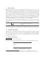
We have followed a few didactical guidelines in writing the course. Learning is best done from
examples, learning is done from practice. The examples are often formatted in two columns,
as follows:2
beginfig(1);
draw unitsquare scaled 1cm;
endfig;
The exercises give you the opportunity to practice METAPOST, instead of only reading about
the program. Compare your answers with the ones in the section ‘Solutions to the Exercises’.
2
A Simple Example
METAPOST is not a WYSIWYG drawing tool like xfig or xpaint. It is a graphic document
preparation system. First, you write a plain text containing graphic formatting commands
into a file by means of your favorite editor. Next, the METAPOST program converts this text
into a PostScript document that you can preview and print. In this section we shall describe
the basics of this process.
2.1
Running METAPOST
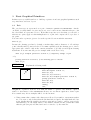
EXERCISE 1
Do the following steps:
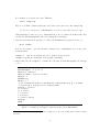
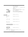
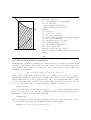
1. Create a text file, say example.mp, that contains the following METAPOST statements:
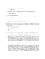
beginfig(1);
draw (0,0)--(10,0)--(10,10)--(0,10)--(0,0);
endfig;
end;
Figure 1: A Simple METAPOST document.
1
2
You can also run METAPOST on a windows platform, e.g., using MikTEXand the WinEdt shell.
On the left is printed the graphic result of the METAPOST code on the right. Here, a square is drawn.
3
For example, you can use the editor XEmacs:
xemacs example.mp
The above UNIX command starts the editor and creates the source file example.mp.
Good advice: always give a METAPOST source file a name with extension .mp.
This will make it easier for you to distinguish the source document from files with other
extensions, which METAPOST will create during the formatting.
2. Generate from this file PostScript code. Here the METAPOST program does the job:
mpost example
It is not necessary to give the filename extension here. METAPOST now creates some
additional files:
example.1 that is a PostScript file can be printed and previewed;
example.log that is a transcript of the graphic formatting.
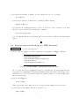
3. Check that the file example.1 contains the following normal Encapsulated PostScript
code:3
%!PS
%%BoundingBox: -1 -1 11 11
%%Creator: MetaPost
%%CreationDate: 2003.05.11:2203
%%Pages: 1
%%EndProlog
%%Page: 1 1
0 0.5 dtransform truncate idtransform setlinewidth pop [] 0 setdash
1 setlinecap 1 setlinejoin 10 setmiterlimit
newpath 0 0 moveto
10 0 lineto
10 10 lineto
0 10 lineto
0 10 lineto
0 0 lineto stroke
showpage
%%EOF
Figure 2: A Simple PostScript Document generated from METAPOST.
3
Notice that the bounding box is larger than you might expect, due to the default width of the line drawing
the square.
4
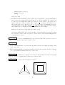
4. Preview the PostScript document on your computer screen, e.g., by typing:
gs example.1
5. Convert the PostScript document into a printable PDF-document:
ps2pdf example.1
It creates the file example.pdf that you can you can view on the computer screen with
the Adobe Acrobat Reader by entering the command:
acroread example.pdf
You can print this file in the usual way. The picture should look like the following small
square:
2.2
Using the Generated PostScript in a LATEX Document
EXERCISE 2
Do the following steps:
1. Create a file, say sample.tex, that contains the following lines of LATEX commands:
\documentclass{article}
\usepackage{graphicx}
\DeclareGraphicsRule{*}{eps}{*}{}
\begin{document}
\includegraphics{example.1}
Figure 3: A Simple LATEX document that includes the image.
Above, we use the extended graphicx package for including the external graphic file that
was prepared by METAPOST. The DeclareGraphicsRule statement causes all file extensions that are not associated with a well-known graphic format to be treated as Encapsulated PostScript files.
2. Typeset the LATEX-file:
latex example
When typesetting is successful, the device independent file sample.dvi is generated.
3. Convert the dvi-file sample.dvi into PostScript code:
dvips sample
5
4. Preview the PostScript code, e.g., by typing:
gs sample.ps
5. Convert the PostScript document sample.ps into a printable PDF document:
ps2pdf sample.ps
It creates the file sample.pdf.
6. You can avoid the intermediate PostScript generation. Just convert the DVI file immediately into a PDF document via the dvipdf command:
dvipdf sample
2.3
The Structure of a METAPOST Document
We shall use the above examples to explain the basic structure of an METAPOST document.
We start with a closer look at the slightly modified METAPOST code in the file example.mp
of our first example:
beginfig(1); % draw a square
draw (0,0)--(10,0)--(10,10)
--(0,10)--(0,0);
endfig;
end;
This example illustrates the following list of general remarks about regular METAPOST files
• It is recommended to end each METAPOST program in a file with extension mp so that
this part of the name can be omitted when invoking METAPOST.
• Each statement in a METAPOST program is ended by a semicolon. Only in cases where
the statement has a clear endpoint, e.g., in the end and endfig statement, you may
omit superfluous semicolons. We shall not do this in this tutorial. You can put two or
more statements on one line as long as they are separated by semicolons. You may also
stretch a statement across several lines of code and you may insert spaces for readability.
• You can add comments in the document by placing a percentage symbol % in front of
the commentary. METAPOST ignores during processing of the document what comes
in a line after the % symbol.
• A METAPOST document normally contains a sequence of beginfig and endfig pairs
with an end statement after the last one. The numeric argument to the beginfig
macro determines the name of the output file that will contain the PostScript code
generated by the next graphic statements before the corresponding endfig command.
In the above case, the output of the draw statement between beginfig(1) en endfig
is written in the file example.1. In general, a METAPOST document consists of one or
more instances of
6
beginfig(figure number );
graphic commands
endfig;
followed by end.
• The draw statement with the points separated by two hyphens (--) draws straight lines
that connect the neighboring points. In the above case for example, the point (0,0)
is connected by straight lines with the point (10,0) and (0,10). The picture is a
1
square with edges of size 10 units, where a unit is 72
of an inch. We shall refer to
this default unit as a ‘PostScript point’ or ‘big point’ (bp) to distinguish it from the
1
of an inch. Other units of measure include
‘standard printer’s point’ (pt), which is 72.27
in for inches, cm for centimeters, and mm for millimeters. For example,
draw (0,0)--(1cm,0)--(1cm,1cm)--(0,1cm)--(0,0);
generates a square with edges of size 1cm. Here, 1cm is shorthand for 1*cm. You may
use 0 instead of 0cm because cm is just a conversion factor and 0cm just multiplies the
conversion factor by zero.
EXERCISE 3
Create a METAPOST file, say exercise3.mp, that generates a circle of
diameter 2cm using the fullcircle graphic object.
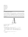
EXERCISE 4
1. Create a METAPOST file, say exercise4.mp, that generates an equilateral triangle with
edges of size 2cm.
2. Extend the METAPOST document such that it generates in a separate file the PostScript
code of an equilateral triangle with edges of size 3cm.
EXERCISE 5
Define your own unit, say 0.5cm, by the statement u=0.5cm; and use this
unit u to generate a regular hexagon with edges of size 2 units.
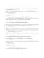
EXERCISE 6
Create the following two pictures:
7
2.4
Numeric Quantities
Numeric quantities in METAPOST are represented in fixed point arithmetic as integer multi1
ples of 65536
= 2−16 and with absolute value less or equal to 4096 = 212 . Since METAPOST
uses fixed point arithmetic, it does not understand exponential notation such as 1.23E4. It
would interpret this as the real number 1.23, followed by the symbol E, followed by the number 4. Assignment of numeric values can be done with the usual := operator. Numeric values
can be shown via the show command.
EXERCISE 7
1. Create a METAPOST file, say exercise7.mp, that contains the following code
numeric p,q,n;
n := 11;
p := 2**n;
q := 2**n+1;
show p,q;
end;
Find out what the result is when you run the above METAPOST program.
2. Replace the value of n in the above METAPOST document by 12 and see what happens
in this case (Hint: press Return to get processing as far as possible). Explain what goes
wrong.
3. Insert at the top of the current METAPOST document the following line and see what
happens now when you process the file.
warningcheck := 0;
The numeric data type is used so often that it is the default type of any non-declared variable.
This explains why n := 10; is the same as numeric n; n := 10; and why you cannot enter
p := (0,0); nor p = (0,0); to define the point, but must use pair p; p := (0,0); or
pair p; p = (0,0); .
2.5
If Processing Goes Wrong
If you make a mistake in the source file and METAPOST cannot process your document
without any trouble, the code generation process is interrupted. In the following exercise,
you will practice the identification and correction of errors.
EXERCISE 8
Deliberately make the following typographical error in the source file
example.mp. Change the line
draw (0,0)--(10,0)--(10,10)--(0,10)--(0,0);
into the following two lines
8
draw (0,0)--(10,0)--(10,10)
draw (10,10)--(0,10)--(0,0);
1. Try to process the document. METAPOST will be unable to do this and the processing
would be interrupted. The terminal window where you entered the mpost command looks
like:
(example.mp ! Extra tokens will be flushed. <to be read again>
addto
draw->addto
.currentpicture.if.picture(EXPR0):also(EXPR0)else:doublepath(EXPR...
<to be read again>
;
l.3 draw (10,10)--(0,10)--(0,0);
?
In a rather obscure way, the METAPOST program notifies the location where it signals
that something goes wrong, viz., at line number 3. However, this does not mean that the
error is necessarily there.
2. There are several ways to proceed after the interrupt. Enter a question mark and you see
your options:
? ?
Type <return> to proceed, S to scroll future error messages,
R to run without stopping, Q to run quietly,
I to insert something, E to edit your file,
1 or ... or 9 to ignore the next 1 to 9 tokens of input,
H for help, X to quit.
?
3. Press Return. LATEX will continue processing and tries to make the best of it. Logging
continues:
[1] )
1 output file written: example.1
Transcript written on example.log.
4. Verify that only the following path is generated:
newpath 0 0 moveto
10 0 lineto
10 10 lineto stroke
5. Format the METAPOST document again, but this time enter the character e. Your default
editor will be opened and the cursor will be at the location where METAPOST spotted
the error. Correct the source file4 , i.e., add a semicolon at the right spot, and give the
METAPOST processing another try.
4
If you have not specified in your UNIX shell the METAPOST editor that you prefer, then the vi-editor
will be started. You can leave this editor by entering ZZ. In the c-shell you can add in the file .cshrc the line
setenv MPEDIT ’xemacs +%d %s’ so that XEmacs is used.
9
3
Basic Graphical Primitives
In this section you will learn how to build up a picture from basic graphical primitives such
as points, lines, and text objects.
3.1
Pair
The pair data type is represented as a pair of numeric quantities in METAPOST. On the
one hand, you may think of a pair, say (1,2), as a location in two-dimensional space. On
the other hand, it represents a vector. From this viewpoint, it is clear that you can add or
subtract two pairs, apply a scalar multiplication to a pair, and compute the dot product of
two pairs.
You can render a point (x,y) as a dot at the specified location with the statement
draw (x,y);
Because the drawing pen has by default a circular shape with a diameter of 1 PostScript
point, a hardly visible point is rendered. You must explicitly scale the drawing pen to a more
appropriate size, either locally in the current statement or globally for subsequent drawing
statements. You can resize the pen for example with a scale factor 4 by
draw (x,y) withpen pencircle scaled 4; % temporary change of pen
or by
pickup pencircle scaled 4; % new drawing pen is chosen
draw (x,y);
EXERCISE 9
Explain the following result:
beginfig(1)
draw unitsquare scaled 70;
draw (10,20);
draw (10,15) scaled 2;
draw (30,40) withpen pencircle scaled 4;
pickup pencircle scaled 8;
draw (40,50);
draw (50,60);
endfig;
end;
Assignment of pairs is often not done with the usual := operator, but with the equation
symbol =. As a matter of fact, METAPOST allows you to use linear equations to define a pair
in a versatile way. A few examples will do for the moment.
• Using a name that consists of the character z followed by a number, a statement such as
z0 = (1,2) not only declares that the left-hand side is equal to the right-hand side, but
it also implies that the variables x0 and y0 exist and are equal to 1 and 2, respectively.
Alternatively, you can assign values to the numeric variable x1 and y1 with the result
that the pair (x1,y1) is defined and can be referred to by the name z1.
10
• A statement like
z1 = -z2 = (3,4);
is equivalent to
z1 = (3,4);
z2 = -(3,4);
• If two pairs, say z1 and z2, are given, you can define the pair, say z3, right in the
middle between these two points by the statement z3 = 1/2[z1,z2].
• When you have declared a pair, say P, then xpart P and ypart P refer to the first and
second coordinate of P, respectively. For example,
pair P;
P = (10,20);
is the same as
pair P;
xpart P = 10;
ypart P = 20;
EXERCISE 10
Verify that when you use a name that begins with z. followed by a
sequence of alphabetic characters and/or numbers, a statement such as z.P = (1,2) not
only declares that the left-hand side is equal to the right-hand side, but it also implies that
the variables x.P and y.P exist and are equal to 1 and 2, respectively. Alternatively, you can
assign values to the numeric variable x.P and y.P, with the result that the pair (x.P,y.P)
is defined and can be referred to by the name z.P.
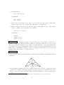
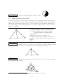
EXERCISE 11
1. Create the following geometrical picture of an acute-angled triangle together with its three
medians5 :
2. The dotlabel command allows you to mark a point with a dot and to position some text
around it. For instance, dotlabel.lft("A",(0,0)); generates a dot with the label A to
the left of the point. Other dotlabel suffices and their meanings are shown in the picture
below:
5
The A-median of a triangle ABC is the line from A to the midpoint of the opposite edge BC.
11
top
lft rt
bot
ulft urt
llft lrt
Use the dotlabel command to put labels in the picture in part 1, so that it looks like
C
B’
A’
B
A
C’
3. Recall that 1/2[z1,z2] denotes the point halfway between the points z1 and z2. Similarly,
1/3[z1,z2] denotes the point on the line connecting the points z1 and z2, one-third away
from z1. For a numeric variable, which is possibly unknown yet, c[z1,z2] is c times of
the way from z1 to —z2—. If you do not want to waste a name for a variable, use the
special name whatever to specify a general point on a line connecting two given points:
whatever[z1,z2];
denotes some point on the line connecting the points z1 and z2. Use this feature to define
the intersection point of the medians, also known as the center of gravity, and extend the
above picture to the one below. Use the label command, which is similar to the dotlabel
command except that it does not draw a dot, to position the character G around the center
of gravity. If necessary, assign labeloffset another value so that the label is further away
from the center of gravity.
C
B’
A’
G
A
B
C’
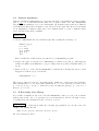
EXERCISE 12
The dir command is a simple way to
√ a point
¡ define
¢ on the unit circle. For
example, dir(30); generates the pair (0.86603,0.5) = ( 12 3, 12 ) . Use the dir command
to generate a regular pentagon.
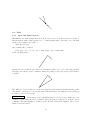
EXERCISE 13
Use the dir command to draw a line in northwest direction through the
point (1, 1) and a line segment through this point that makes an angle of 30 degrees with the
line. Your picture should look like
12
3.2
Path
3.2.1
Open and Closed Curves
METAPOST can draw straight lines as well as curved ones. You have already seen that a
draw statement with points separated by -- draws straight lines connecting one point with
another. For example, the result of
draw p0--p1--p2;
after defining three points by
pair p[];
p0 = (0,0);
p1 = (2cm,3cm);
p2 = (3cm,2cm);
is the following picture.
Closing the above path is done either by extending it with --z0 or by connecting the first
and last point via the cycle command. Thus, the path p0--p1--p2--cycle, when drawn,
looks like
The difference between these two methods is that the path extension with the starting point
only has the optical effect of closing the path. This means that only with the cycle extension
it really becomes a closed path.
EXERCISE 14
Verify that you can only fill the interior of a closed curve with some color
or shade of gray, using the fill command, when the path is really closed with the cycle
command. The gray shading is obtained by the directive withcolor c*white, where c is a
number between 0 and 1.
13
3.2.2
Straight and Curved Lines
Compare the pictures from the previous subsection with the following ones, which show
curves6 through the same points.
u := 1cm;
pair p[];
p0 = (0,0); p1 = (2u,3u); p2 = (3u,2u);
beginfig(1);
draw p0..p1..p2; % draw open curve
for i=0 upto 2:
draw p[i] withpen pencircle scaled 3;
endfor; % draw defining points
endfig;
beginfig(2);
draw p0..p1..p2..cycle; % draw closed curve
for i=0 upto 2:
draw p[i] withpen pencircle scaled 3;
endfor; % draw defining points
endfig;
end;
Just use -- where you want straight lines and .. where you want curves.
beginfig(1);
u := 1cm;
pair p[];
p0 = (0,0); p1 = (2u,3u); p2 = (3u,2u);
draw p0--p1..p2..cycle;
for i=0 upto 2:
draw p[i] withpen pencircle scaled 3;
endfor;
endfig;
end;
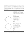
3.2.3
Construction of Curves
When METAPOST draws a smooth curve through a sequence of points, each pair of consecutive
points is connected by a cubic Bézier curve, which needs, in order to be determined, two
intermediate control points in addition to the end points. The points on the curved segment
from points p0 to p1 with post control point c0 and pre control point c1 are determined by
the formula
p(t) = (1 − t)3 p0 + 3(1 − t)2 tc0 + 3(1 − t)t2 c1 + t3 p1 ,
where t ∈ [0, 1]. METAPOST automatically calculates the control points such that the segments have the same direction at the interior knots. In the figure below, the additional
6
the curves through the three points are a circle or a part of the circle
14
control points are drawn as gray dots and connected to their parent point with gray line
segments. The curve moves from the starting point in the direction of the post control point,
but possibly bends after a while in another direction. The further away the post control point
is, the longer the curve keeps this direction. Similarly, the curve arrives at a point coming
from the direction of the pre control point. The further away the pre control point is, the
earlier the curve gets this direction. It is as if the control points pull their parent point in
a certain direction and the further away a control point is, the stronger it pulls. By default
in METAPOST, the incoming and outgoing direction at a point on the curve are the same so
that the curve is smooth.
u := 1.25cm;
color gray; gray := 0.6white;
pair p[];
p0 = (0,0); p1 = (2u,3u); p2 = (3u,2u);
def drawpoint(expr z, c) = draw z
withpen pencircle scaled 3 withcolor c;
enddef;
beginfig(1);
path q; q := p0..p1..p2;
for i=0 upto length(q):
drawpoint(point i of q, black);
p3 := precontrol i of q;
p4 := postcontrol i of q;
draw p3--p4 withcolor gray;
drawpoint(p3, gray);
drawpoint(p4, gray);
endfor;
draw q;
endfig;
beginfig(2);
path q; q := p0..p1..p2..cycle;
for i=0 upto length(q):
drawpoint(point i of q, black);
p3 := precontrol i of q;
p4 := postcontrol i of q;
draw p3--p4 withcolor gray;
drawpoint(p3, gray);
drawpoint(p4, gray);
endfor;
draw q;
endfig;
end;
Do not worry when you do not understand all details of the above METAPOST program. It
contains features and programming constructs that will be dealt with later in the tutorial.
15
There are various ways of controlling curves:
• Vary the angles at the start and end of the curve with one of the keywords up, down,
left, and right, or with the dir command.
• Specify the requested control points manually.
• Vary the inflection of the curve with tension and curl. tension influences the curvature, whereas curl influences the approach of the starting and end points.
pair p[]; p0:=(0,0); p1:=(1cm,1cm);
def drawsquare = draw unitsquare
scaled 1cm withcolor 0.7white;
enddef;
beginfig(1);
drawsquare; drawarrow p0..p1;
endfig;
beginfig(2);
drawsquare; drawarrow p0{right}..p1;
endfig;
beginfig(3);
drawsquare; drawarrow p0{up}..p1;
endfig;
beginfig(4);
drawsquare; drawarrow p0{left}..p1;
endfig;
beginfig(5);
drawsquare; drawarrow p0{down}..p1;
endfig;
beginfig(6);
drawsquare; drawarrow p0{dir(-45)}..p1;
endfig;
beginfig(7);
drawsquare; drawarrow p0..
controls (0,1cm) and (1cm,0) ..p1;
endfig;
16
beginfig(8);
drawsquare; drawarrow p0{curl 80}..
(0,-1cm)..{curl 8}p1;
endfig;
beginfig(9);
drawsquare; drawarrow p0..tension(2)
..(0,1cm)..p1;
endfig;
end;
The METAPOST operators --, ---, and ... have been defined in terms of curl and tension
directives as follows:
def -- = {curl 1}..{curl 1}
enddef;
def --- = .. tension infinity .. enddef;
def ... = .. tension atleast 1 .. enddef;
The meaning of ... is “choose an inflection-free path between the points unless the endpoint
directions make this impossible”. The meaning of --- is “get a smooth connection between
a straight line and the rest of the curve”.
pair p[]; p0:=(0,0); p1:=(1cm,1cm);
def drawsquare = draw unitsquare scaled 1cm
withcolor 0.7white;
enddef;
beginfig(1);
drawsquare; drawarrow p0---(1.5cm,0)..p1;
endfig;
beginfig(2);
drawsquare; drawarrow p0...(1.5cm,0)..p1;
endfig;
end;
The above examples were also meant to give you the impression that you can draw in METAPOST almost any curve you wish.
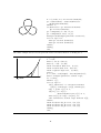
EXERCISE 15
EXERCISE 16
Draw an angle of 40 degrees that looks like
Draw a graph that looks like
17
EXERCISE 17
3.3
Draw the Yin-Yang symbol7 that looks like
Angle and Direction Vector
In a previous exercise you have already seen that the dir command generates a pair that is a
point on the unit circle at a given angle with the horizontal axis. The inverse of dir is angle,
which takes a pair, interprets it as a vector, and computes the two-argument arctangent, i.e.,
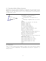
it gives the angle corresponding with the vector. In the example below we use it to draw a
bisector of a triangle.
pair A, B, C, C’;
u := 1cm; A=(0,0); B=(5u,0); C=(2u,3u);
C’ = whatever[A,B] = C + whatever*dir(
1/2*angle(A-C)+1/2*angle(B-C));
beginfig(1)
draw A--B--C--cycle; draw C--C’;
dotlabel.lft("A",A); dotlabel.urt("B",B);
dotlabel.top("C",C); dotlabel.bot("C’",C’);
endfig;
end;
C
B
A
C’
EXERCISE 18
Change the above picture to the following geometrical diagram, which
illustrates better that a bisector is actually drawn for the acute-angled triangle.
C
B
A
C’
EXERCISE 19
Draw a picture that shows all the bisectors of a acute-angled triangle.
Your picture should look like
C
B’
A
A’
I
C’
7
B
See www.chinesefortunecalendar.com/YinYang.htm for details about the symbol.
18
In this way, it illustrates that the bisectors of a triangle go through one point, the so-called
incenter, which is the center of the inner circle of the triangle.
3.4
Arrow
The drawarrow command draws the given path with an arrowhead at the end. For doubleheaded arrows, simply use the drawdblarrow command. A few examples:
beginfig(1);
drawarrow (0,0)--(60,0);
drawarrow reverse((0,-20)--(60,-20))
withpen pencircle scaled 2;
drawdblarrow (0,-40)--(60,-40);
drawarrow (0,-65){dir(30)}..
{dir(-30)}(60,-65);
drawarrow (0,-90){dir(-30)}..{up}(60,-90)..
{dir(-150)}cycle;
endfig;
end;
If you want arrowheads of different size, you can change the arrowhead length through the
variable ahlength (4bp by default) and you can control the angle at the tip of the arrowhead
with the variable ahangle (45 degrees by default). You can also completely change the
definition of the arrowhead procedure. In the example below, we draw a curve with an arrow
symbol along the path. As a matter of fact, the path is drawn in separate pieces that are
joined together with the & operator.
beginfig(1);
save arrowhead;
vardef arrowhead(expr p) =
save A,u,a,b; pair A,u; path a,b;
A := point length(p)/2 of p;
u := unitvector(direction length(p)/2 of p);
a := A{-u}..(A - ahlength*u rotated 30);
b := A{-u}..(A - ahlength*u rotated -30);
(a & reverse(a) & b & reverse(b))--cycle
enddef;
u:=2cm; ahlength:=0.3cm;
drawarrow (0,0)..(u,u)..(-u,u);
endfig; end;
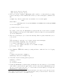
3.5
Circle, Ellipse, Square, and Rectangle
You have already seen that you can draw a circle through three points z0, z1, and z2, that do
not lie on a straight line with the statement draw z0..z1..z2..cycle;. But METAPOST also
provides predefined paths to build circles and circular disks or parts of them. Similarly, you
can draw a rectangle once the four corner points, say z0, z1, z2, and z3, are known with the
19
statement draw z0--z1--z2--z3--cycle;. The path (0,0)--(1,0)--(1,1)--(0,1)--cycle
is in METAPOST predefined as unitsquare.
Path
fullcircle
halfcircle
quartercircle
unitsquare
Definition
circle with diameter 1 and center (0, 0).
upper half of fullcircle
first quadrant of fullcircle
(0,0)--(1,0)--(1,1)--cyle
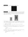
You can construct from these basic paths any circle, ellipse, square, or rectangle by rotating
(rotated operator), by scaling (operators scaled, xscaled, and yscaled), and/or by translating the graphic object (shifted operator). Keep in mind that the ordering of operators
has a strong influence on the final shape. But pictures say more than words. The diagram
is drawn with the following METAPOST code.
beginfig(1);
u := 24; % 24 = 24bp = 1/3 inch
for i=-1 upto 9: draw (i*u,4u)--(i*u,-3u) withcolor 0.7white; endfor;
for i=-3 upto 4: draw (-u,i*u)--(9u,i*u) withcolor 0.7white; endfor;
dotlabel("",origin); % the grid with reference point (0,0) has been drawn
draw fullcircle scaled u;
draw halfcircle scaled u shifted (2u,0);
draw quartercircle scaled u shifted (4u,0);
draw fullcircle xscaled 2u yscaled u shifted (6u,0);
draw fullcircle xscaled 2u yscaled u rotated -45 shifted (8u,0);
fill fullcircle scaled u shifted (0,-2u);
fill halfcircle--cycle scaled u shifted (2u,-2u);
path quarterdisk; quarterdisk := quartercircle--origin--cycle;
fill quarterdisk scaled u shifted (4u,-2u);
fill quarterdisk scaled u rotated -45 shifted (6u,-2u);
fill quarterdisk scaled u shifted (6u,-2u) rotated 45;
fill quarterdisk rotated -90 scaled 2u shifted (8u,3u);
fill unitsquare scaled u shifted (0,2u);
20
fill unitsquare xscaled u yscaled 3/2u shifted (2u,2u);
endfig;
end;
3.6
Text
You have already seen how the dotlabel command can be used to draw a dot and a label in
the neighborhood of the dot. If you do not want the dot, simply use the label command:
label.suffix (string expression, pair );
It uses of the same suffices as the dotlabel command to position the label relative to the
given pair. No suffix means that the label is printed at the specified location. The directives
rt (right), urt (upper right), top (top), ulft (upper left), lft (left), llft (lower left), bot
(bottom), lrt (lower right) can be used to specify the relative position of the label to the given
pair. The distance from the pair to the label is set by the numeric variable labeloffset.
The commands label and dotlabel both use a string expression for the label text and
typeset it in the default font, which is likely to be "cmr10" and which can changed through
the variables defaultfont and defaultscale. For example,
defaultfont := "tir";
defaultscale := 12pt/fontsize(defaultfont);
makes labels come out as Adobe Times-Roman at about 12 points.
Until now the string expression in a text command has only been a string delimited by double
quotes (optionally joined to another string via the concatenation operator &). But you can
also bracket the text with btex and etex (do not put it in quotes this time) and pass it to
TEX for typesetting. This allows you to use METAPOST in combination with TEX for building
complex labels. Let us begin with a simple example:
2
√
3
1
beginfig(1);
z0 = (0,0); z1 = (sqrt(3)*cm,0);
z2 = (sqrt(3)*cm,1cm);
draw z0--z1--z2--cycle;
label.bot(btex $\sqrt{3}$ etex, 1/2[z0,z1]);
label.rt(btex 1 etex, 1/2[z1,z2]);
label.top(btex 2 etex, 1/2[z0,z2]);
endfig;
end;
Whenever the METAPOST program encounters btex typesetting commands etex, it suspends
the processing of the input in order to allow TEX to typeset the commands and the dvitomp
preprocessor to translate the typeset material into a picture expression that can be used in
a label or dotlabel statement. The generated low level METAPOST code is placed in a file
with extension .mpx. Hereafter METAPOST resumes its work.
We speak about a picture expression that is created by typesetting commands because it is
a graphic object to which you can apply transformation. This is illustrated by the following
example, in which we use diagonal curly brackets and text.
21
}
2
{
{
√
3
1
beginfig(1);
z0 = (0,0); z1 = (sqrt(3)*cm,0);
z2 = (sqrt(3)*cm,1cm);
draw z0--z1--z2--cycle;
label.bot(btex $\lbrace$ etex rotated 90
xscaled 5 yscaled 1.4, 1/2[z0,z1]);
label.rt((btex $\rbrace$ etex) xscaled 1.3
yscaled 3, 1/2[z1,z2]);
label(btex $\lbrace$ etex xscaled 1.5 yscaled 5.7
rotated -60, 1/2[z0,z2] + dir(120)*2mm);
labeloffset:=3.5mm;
label.bot(btex $\sqrt{3}$ etex, 1/2[z0,z1]);
label.rt(btex 1 etex, 1/2[z1,z2]);
label(btex 2 etex, 1/2[z0,z2]+dir(120)*5mm);
endfig;
end;
Until now we have only used plain TEX commands. But what if you want to run another
TEX-version? The following example shows how you can use a verbatimtex.....etex block
to specify that LATEX is used and which style and/or packages are chosen.
1
√
3
1
2
verbatimtex
%&latex
\documentclass{article}
\begin{document}
etex
beginfig(1);
z0 = (0,0); z1 = (sqrt(3)*cm,0);
z2 = (sqrt(3)*cm,1cm);
draw z0--z1--z2--cycle;
label.bot(btex $\sqrt{3}$ etex, 1/2[z0,z1]);
label.rt(btex $\frac{1}{2}$ etex, 1/2[z1,z2]);
label.top(btex 1 etex, 1/2[z0,z2]);
endfig;
end;
One last remark about using LATEX: Between btex and etex, you cannot use displayed math
mode such as $$\frac{x}{x+1}$$. You must use $\displaystyle \frac{x}{x+1}$ instead.
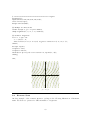
Let us use what we have learned so far in this chapter in a more practical example, viz.,
ex
drawing the graph of the function x 7→
from 0 to 5 with the vertical axis in a logarithmic
1+x
scale. The picture looks as follows:
22
100
graph of x 7→
logarithmic scale
50
ex
1+x
10
5
1
0
1
2
3
4
linear scale
It is generated by the following METAPOST code:
verbatimtex
%&latex
\documentclass{article}
\begin{document}
etex
% some function definitions
vardef exp(expr x) = (mexp(256)**x) enddef;
vardef ln(expr x) = (mlog(x)/256) enddef;
vardef log(expr x) = (ln(x)/ln(10)) enddef;
vardef f(expr x) = (exp(x)/(1+x)) enddef;
ux := 1cm; uy := 4cm;
beginfig(1)
numeric xmin, xmax, ymin, ymax;
xmin := 0; xmax := 6;
ymin := 0; ymax := 2;
% draw axes
draw (xmin,0)*ux -- (xmax+1/2,0)*ux;
draw (0,ymin)*uy -- (0,ymax+1/10)*uy;
% draw tickmarks and labels on horizontal axis
for i=0 upto xmax:
draw (i,-0.05)*ux--(i,0.05)*ux;
label.bot(decimal(i),(i,0)*ux);
endfor;
23
5
6
% draw tickmarks and labels on vertical axis
for i=2 upto 10:
draw (-0.01,log(i))*uy--(0.01,log(i))*uy;
draw (-0.01,log(10*i))*uy--(0.01,log(10*i))*uy;
endfor;
for i=0 upto 2: label.lft(decimal(10**i), (0,i)*uy); endfor;
for i=0 upto 1: label.lft(decimal(5*(10**i)), (0,log(5*(10**i)))*uy); endfor;
% compute and draw the graph of the function
xinc := 0.1;
path pts_f;
pts_f := (xmin*ux,log(f(xmin))*uy)
for x=xmin+xinc step xinc until xmax:
.. (x*ux,log(f(x))*uy)
endfor;
draw pts_f withpen pencircle scaled 2;
% draw title
label(btex graph of $\displaystyle x\mapsto\frac{e^x}{1+x}$ etex, (2ux,1.7uy));
% draw axis explanation
labeloffset := 0.5cm;
label.bot(btex linear scale etex, (3,0)*ux);
label.lft(btex logarithmic scale etex rotated(90), (0,1)*uy);
endfig;
end;
The above code needs some explanation.
First of all, METAPOST does not know about the exponential or logarithmic function. But you
can easily define these functions with the help of the built-in functions mepx(x) = exp(x/256)
and mlog(x) = 256 ln x . Note that we have reserved the name log for the logarithm with
base 10 in the above program.
As you will see later in this tutorial, METAPOST has several repetition control structures.
Here we apply the for loop to draw tick marks and labels on the axes and to compute the
path of the graph. The basic form is:
for counter = start step stepsize until finish :
loop text
endfor;
Instead of step 1 until, you may use the keyword upto. downto is another word for
step -1 until.
In the following code snippet
for i=0 upto xmax:
draw (i,-0.05)*ux--(i,0.05)*ux;
label.bot(decimal(i),(i,0)*ux);
endfor;
24
the input lines are two statements, viz., one to draw tick marks and the other to put a label.
We use the decimal command to convert the numeric variable i into a string so that we can
use it in the label statement. The following code snippet
pts_f := (xmin*ux,log(f(xmin))*uy)
for x=xmin+xinc step xinc until xmax:
.. (x*ux,log(f(x))*uy)
endfor;
shows that you can also use the for loop to build up a single statement. The input lines
within the for loop are pieces of a path definition. This mode of creating a statement may
look strange at first sight, but it is an opportunity given by the fact that METAPOST consists
more or less of two part, viz., a preprocessor and a PostScript generator. The preprocessor
only reads from the input stream and prepares input for the PostScript generator.
EXERCISE 20
Draw the graph of the function x 7→
picture should look like
√
x on the interval (0, 2). Your
2
y=
y 1
0
0
1
2
x
√
x
3
4
Your METAPOST code should be such that only a minimal change in the code is required to
draw the graph on a different domain, say [0, 3].
EXERCISE 21
Draw the following picture in METAPOST. The dashed lines can be
drawn by adding dashed evenly at the end of the draw statement.
C
ib
a + ib = z
|z|
{
φ
a
0
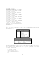
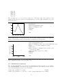
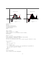
EXERCISE 22
The annual beer consumption in the Netherlands in the period 1980–2000
is listed below.
year
liter
1980
86
1985
85
1990
91
Draw the following graph in METAPOST.
25
1995
86
2000
83
beer consumption (liter)
92
90
88
86
84
82
1980 1985 1990 1995 2000
year
4
Style Directives
In this section we explain how you can alter the appearance of graphics primitives, e.g., allowing certain lines to be thicker and others to be dashed, using different colors, and changing
the type of the drawing pen.
4.1
Dashing
Examples show you best how the specify a dash pattern when drawing a line or curve.
beginfig(1);
path p; p := (0,0)--(102,0);
def drawit (suffix p)(expr pattern) =
draw p dashed pattern;
p := p shifted (0,-13);
enddef;
drawit(p, withdots);
drawit(p, withdots scaled 2);
drawit(p, evenly);
drawit(p, evenly scaled 2);
drawit(p, evenly scaled 4);
drawit(p, evenly scaled 6);
p := (0,-150)--(102,-150);
def shiftit (suffix p)(expr s) =
draw p dashed evenly scaled 4 shifted s;
dotlabel("",point 0 of p);
dotlabel("",point 1 of p);
p := p shifted (0,-13);
enddef;
shiftit(p, (0,0));
shiftit(p, (4bp,0));
shiftit(p, (8bp,0));
shiftit(p, (12bp,0));
shiftit(p, (16bp,0));
shiftit(p, (20bp,0));
26
picture dd; dd :=
dashpattern(on 6bp off 2bp on 2bp off 2bp);
draw (0,-283)--(102,-283) dashed dd;
draw (0,-296)--(102,-296) dashed dd scaled 2;
endfig;
end;
In general, the syntax for dashing is
draw path dashed dash pattern;
You can define a dash pattern with the dashpattern function whose argument is a sequence
of on/off distances. Predefined patterns are:
evenly
= dashpattern(on 3 off 3); % equal length dashes
withdots = dashpattern(off 2.5 on 0 off 2.5); % dotted lines
4.2
Coloring
The color data type is represented as a triple (r, g, b) that specifies a color in the RGB
color system. Each of r, g, and b must be a number between 0 and 1, inclusively, representing
fractional intensity of red, green, or blue, respectively. Predefined colors are:
red
= (1,0,0);
black = (0,0,0);
green = (0,1,0);
white = (1,1,1);
blue = (0,0,1);
A shade of gray can be specified most conveniently by multiplying the white color with some
scalar between 0 and 1. The syntax of using a color in a graphic statement is:
withcolor color expression;
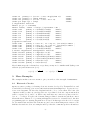
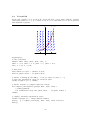
Let us draw two color charts:
RGB(r,g,0)
1
0.9
0.8
0.7
g
0.6
0.5
0.4
0.3
0.2
0.1
0
0 0.1 0.2 0.3 0.4 0.5 0.6 0.7 0.8 0.9 1
r
beginfig(1);
u := 1/2cm;
defaultscale := 10pt/fontsize(defaultfont);
beginfig(1);
path sqr; sqr := unitsquare scaled u;
for i=0 upto 10:
label.bot(decimal(i/10), ((i+1/2)*u,0));
label.lft(decimal(i/10), (0,(i+1/2)*u));
for j=0 upto 10:
fill sqr shifted (i*u,j*u)
withcolor (i*0.1, j*0.1,0);
draw sqr shifted (i*u,j*u); % draw grid
endfor;
endfor;
label.bot("r",(6u,-2/3u));
label.lft("g",(-u,6u));
label.top("RGB(r,g,0)", (6u,11u));
endfig; end;
27
beginfig(2);
draw (-u,-u)--(11u,-u)--(11u,u)--(-u,u)
--cycle; % bounding box
pickup pencircle scaled 1/2u;
for i=0 upto 10:
draw (i*u,0) withcolor i*0.1*white;
endfor;
endfig;
end;
EXERCISE 23
Compare the linear conversion from color to gray, defined by the function
(r + g + b)
× (1, 1, 1)
3
with the following conversion formula used in black and white television:
(r, g, b) 7→
(r, g, b) 7→ (0.30r + 0.59g + 0.11b) × (1, 1, 1) .
4.3
Specifying the Pen
In METAPOST you can define your drawing pen for specifying the line thickness or for calligraphic effects. The statement
draw path withpen pen expression;
causes the chosen pen to be used to draw the specified path. This is only a temporary pen
change. The statement
pickup pen expression;
causes the given pen to be used in subsequent draw statements. The default pen is circular
with a diameter of 0.5 bp. If you want to change the line thickness, simply use the following
pen expression:
pencircle scaled numeric expression;
You can create an elliptically shaped and rotated pen by transforming the circular pen. An
example:
beginfig(1);
pickup pencircle xscaled 2bp yscaled 0.25bp
rotated 60 withcolor red;
for i=10 downto 1:
draw 5(i,0)..5(0,i)..5(-i,0)
..5(0,-i+1)..5(i-1,0);
endfor;
endfig;
end;
28
In the following example we define a triangular shaped pen. It can be used to plot data points
as triangles instead of dots. For comparison we draw a large triangle with both the triangular
and the default circular pen.
beginfig(1);
path p; p := dir(-30)--dir(90)--dir(210)--cycle;
pen pentriangle;
pentriangle := makepen(p);
draw origin withpen pentriangle scaled 2;
draw (p scaled 1cm) withpen pentriangle scaled 4;
draw (p scaled 2cm) withpen pencircle scaled 8;
endfig;
end;
4.4
Setting Drawing Options
The function drawoptions allows you to change the default settings for drawing. For example,
if you specify
drawoptions(dashed evenly withcolor red);
then all draw statements produce dashed lines in red color, unless you overrule the drawing
setting explicitly. To turn off drawoptions all together, just give an empty list:
drawoptions();
As a matter of fact, this is done automatically by the beginfig macro.
5
Transformations
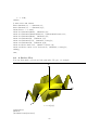
A very characteristic technique with METAPOST, which we applied already in many of the
previous examples, is creating a graphic and then using it several times with different transformations. METAPOST has the following built-in operators for scaling, rotating, translating,
reflecting, and slanting:
(x, y) shifted (a, b) = (x + a, y + b) ;
(x, y) rotated (θ) = (x cos θ − y sin θ, x sin θ + y cos θ) ;
¡
¢
(x, y) rotatedaround (a, b), θ = (x cos θ − y sin θ + a(1 − cos θ) + b sin θ,
x sin θ + y cos θ + b(1 − cos θ) − a sin θ) ;
(x, y) slanted a = (x + ay, y) ;
(x, y) scaled a = (ax, ay) ;
(x, y) xscaled a = (ax, y) ;
(x, y) yscaled a = (x, ay) ;
(x, y) zscaled (a, b) = (ax − by, bx + ay) .
The effect of the translation and most scaling operations is obvious. The following playful
example, in which the formula eπi = −1 is drawn in various shapes, serves as an illustration
of most of the listed transformations.
29
beginfig(1);
pair s; s=(0,-2cm);
def drawit(expr p) =
draw p shifted s; s := s shifted (0,-2cm);
enddef;
picture pic;
draw btex $e^{\pi i}=-1$ etex;
draw bbox currentpicture withcolor 0.6white;
pic := currentpicture;
draw pic shifted (1cm, -1cm);
pic := pic scaled 1.5; drawit(pic);
% work with the enlarged base picture
eπi = −1
eπi = −1
eπi = −1
drawit(pic scaled -1);
eπi = −1
πi
e
=
−1
drawit(pic rotated 30);
e πi = −1
drawit(pic slanted 0.5);
eπi = −1
drawit(pic slanted -0.5);
eπi = −1
eπi = −1
e πi =
drawit(pic xscaled 2);
drawit(pic yscaled -1);
−1
drawit(pic zscaled (2, -0.5));
endfig;
end;
30
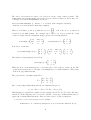
The effect of rotated θ is rotation of θ degrees about the origin counter-clockwise. The
transformation rotatedaround(p, θ) rotates θ degrees counter-clockwise around point p. Accordingly, it is defined in METAPOST as follows:
def rotatedaround(expr p, theta) = % rotates theta degrees around p
shifted -p rotated theta shifted p enddef;
 
x
When you identify a point (x, y) with the 3-vector y , each of the above operations is
1
described by an affine matrix. For example, the rotation of θ degrees around the origin
counter-clockwise and the translation with (a, b) have the following matrices:




cos θ − sin θ 0
1 0 a
rotated(θ) =  sin θ cos θ 0 ,
translated(a, b) = 0 1 b  .
0
0
1
0 0 1
It is easy to verify that

 
 

1 0 a
cos θ − sin θ 0
1 0 −a
¡
¢
rotatedaround (a, b), θ = 0 1 b  ·  sin θ cos θ 0 · 0 1 −b  .
0 0 1
0
0
1
0 0 1
The matrix of zscaled(a,b) is as follows:


a −b 0
zscaled(a, b) =  b a 0 .
0 0 1
Thus, the effect of zscaled(a,b) is to rotate and scale so as to map (1,0) into (a,b). The
operation zscaled can also be thought of as multiplication of complex numbers. The picture
on the next page illustrates this.
The general form of an affine matrix T is


Txx Txy Tx
T = Tyx Tyy Ty  .
0
0
1
The corresponding transformation in the two-dimensional space is
(x, y) 7→ (Txx x + Txy y + Tx , Tyx x + Tyy y + Ty ).
This mapping is completely determined by the sextuple (Tx , Ty , Txx , Txy , Tyx , Tyy ). The information about the mapping can be stored in a variable of data type transform and then be
applied in a transformed statement. There are three ways to define a transform:
• In terms of basic transformations. For example,
transform T; T = identity shifted (-1,0) rotated 60 shifted (1,0);
31
defines the transformation T as a composition of translating with vector (−1, 0), rotating
around the origin over 60 degrees, and translating with a vector (1, 0).
• Specifying the sextuple (Tx , Ty , Txx , Txy , Tyx , Tyy ). The six parameters than define a
transformation T can be referred to directly as xpart T, ypart T, xxpart T, xypart T,
yxpart T, and yypart T. Thus,
transform T;
xpart T = ypart T = 1;
xxpart T = yypart T = 0;
xypart T = yxpart T = -1;
defines a transformation, viz., the reflection in the line through (1, 0) and (0, 1).
zw
w
z
0
1
beginfig(1);
pair z; z := (2,1)*cm;
pair w; w := (7/4,3/2)*cm;
pair zw; zw := (z zscaled w) / cm;
draw
draw
draw
draw
(-0.5,0)*cm--(3,0)*cm;
(0,-0.5)*cm--(0,5.5)*cm;
(1,0)*cm--z; draw (0,0)--z; draw (0,0)--w;
(0,0)--zw; draw w--zw;
def drawangle(
expr endofa, endofb, common, length) =
save tn; tn :=
turningnumber(common--endofa--endofb--cycle);
draw (unitvector(endofa-common){(endofa-common)
rotated (tn*90)} .. unitvector(endofb-common))
scaled length shifted common withcolor 0.3white;
enddef;
drawangle((1,0)*cm, z, (0,0), 0.4cm);
drawangle(w, zw, (0,0), 0.4cm);
drawangle((0,0), z, (1,0)*cm, 0.2cm);
drawangle((0,0), z, (1,0)*cm, 0.15cm);
drawangle((0,0), zw, w, 0.2cm);
drawangle((0,0), zw, w, 0.15cm);
label.llft(btex $0$ etex,(0cm,0cm));
label.lrt(btex $1$ etex,(1cm,0cm));
label.rt(btex $z$ etex, z);
label.rt(btex $w$ etex, w);
label.rt(btex $zw$ etex, zw);
endfig;
end;
32
• Specifying the images of three points. It is possible to apply an unknown transform to
a known pair and use the result in a linear equation. For example,
transform T;
(1,0) transformed T = (1,0);
(0,1) transformed T = (0,1);
(0,0) transformed T = (1,1);
defines the reflection in the line through (1, 0) and (0, 1).
The built-in transformation reflectedabout(p,q), which reflects about the line connecting
the points p and q, is defined by a combination of the last two techniques:
def reflectedabout(expr p,q) = transformed
begingroup
transform T_;
p transformed T_ = p; q transformed T_ = q;
xxpart T_ = -yypart T_; xypart T_ = yxpart T_; % T_ is a reflection
T_
endgroup
enddef;
Given a transformation T, the inverse transformation is easily defined by inverse(T).
We end with another playful example of an iterative graphic process.
beginfig(1);
pair A,B,C; u:=3cm;
A=u*dir(-30); B=u*dir(90); C=u*dir(210);
transform T;
A transformed T = 1/6[A,B];
B transformed T = 1/6[B,C];
C transformed T = 1/6[C,A];
path p; p = A--B--C--cycle;
for i=0 upto 60:
draw p; p:= p transformed T;
endfor;
endfig;
end;
EXERCISE 24
Using transformations, construct the following picture:
33
6
Advanced Graphics
In this section we deal with fine points of drawing lines and with more advanced graphics. This
will allow you to create more professional-looking graphics and more complicated pictures.
6.1
Joining Lines
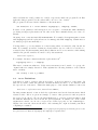
In the last example of the section on pen styles you may have noticed that lines are joined
by default such that line joints are normally rounded. You can influence the appearances of
the lines by the two internal variables linejoin and linecap. The picture below shows the
possibilities.
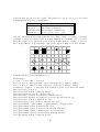
18
20
21
23
24
26
19
22
25
linejoin=beveled
linejoin=beveled
linejoin=beveled
linecap=butt
linecap=rounded
linecap=squared
9
11
12
14
15
17
10
13
16
linejoin=rounded
linecap=butt
linejoin=rounded
linecap=rounded
linejoin=rounded
linecap=squared
0
2
3
5
6
8
1
4
7
linejoin=mitered
linecap=butt
linejoin=mitered
linecap=rounded
linejoin=mitered
linecap=squared
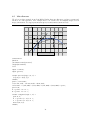
This picture can be produced by the following METAPOST code
beginfig(1);
for i=0 upto 2:
for j=0 upto 2:
34
z[3i+9j]=(150i, 150j);
z[3i+9j+1]=(150i+50,150j-50);
z[3i+9j+2]=(150i+100,150j);
endfor;
endfor;
drawoptions(withpen pencircle scaled 24 withcolor 0.75white);
linejoin := mitered; linecap := butt;
draw z0--z1--z2;
linejoin := mitered; linecap := rounded; draw z3--z4--z5;
linejoin := mitered; linecap := squared; draw z6--z7--z8;
linejoin := rounded; linecap := butt;
draw z9--z10--z11;
linejoin := rounded; linecap := rounded; draw z12--z13--z14;
linejoin := rounded; linecap := squared; draw z15--z16--z17;
linejoin := beveled; linecap := butt;
draw z18--z19--z20;
linejoin := beveled; linecap := rounded; draw z21--z22--z23;
linejoin := beveled; linecap := squared; draw z24--z25--z26;
%
drawoptions();
for i=0 upto 26: dotlabel.bot(decimal(i), z[i]); endfor;
labeloffset := 25pt; label.bot("linejoin=mitered", z1);
labeloffset := 40pt; label.bot("linecap=butt",
z1);
labeloffset := 25pt; label.bot("linejoin=mitered", z4);
labeloffset := 40pt; label.bot("linecap=rounded", z4);
labeloffset := 25pt; label.bot("linejoin=mitered", z7);
labeloffset := 40pt; label.bot("linecap=squared", z7);
%
labeloffset := 25pt; label.bot("linejoin=rounded", z10);
labeloffset := 40pt; label.bot("linecap=butt",
z10);
labeloffset := 25pt; label.bot("linejoin=rounded", z13);
labeloffset := 40pt; label.bot("linecap=rounded", z13);
labeloffset := 25pt; label.bot("linejoin=rounded", z16);
labeloffset := 40pt; label.bot("linecap=squared", z16);
%
labeloffset := 25pt; label.bot("linejoin=beveled", z19);
labeloffset := 40pt; label.bot("linecap=butt",
z19);
labeloffset := 25pt; label.bot("linejoin=beveled", z22);
labeloffset := 40pt; label.bot("linecap=rounded", z22);
labeloffset := 25pt; label.bot("linejoin=beveled", z25);
labeloffset := 40pt; label.bot("linecap=squared", z25);
%
endfig;
end;
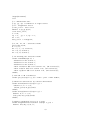
By setting the variable miterlimit, you can influence the mitering of joints. The next
example demonstrates that the value of this variable acts as a trigger.
beginfig(1);
for i=0 upto 2:
35
z[3i]=(150i,0); z[3i+1]=(150i+50,-50); z[3i+2]=(150i+100,0);
endfor;
drawoptions(withpen pencircle scaled 24pt);
labeloffset:= 25pt;
linejoin := mitered; linecap:=butt;
for i=0 upto 2:
miterlimit := i;
draw z[3i]--z[3i+1]--z[3i+2];
label.bot("miterlimit=" & decimal(miterlimit), z[3i+1]);
endfor;
endfig;
end;
miterlimit=0
6.2
miterlimit=1
miterlimit=2
Building Cycles
In previous examples you have seen that intersection points of straight lines can be specified
by linear equations. A more direct way to deal with path intersection is via the operator
intersectionpoint. So, given four points z1, z3, z3, and z4 in general position, you can
specify the intersection point z5 of the line between z1 and z2 and the line between z3 and
z4 by
z5 = z1--z2 intersectionpoint z3--z4;
You do not need to rely on setting up linear equations with
z5 = whatever[z1,z2] = whatever[z3,z4];
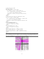
The strength of the intersection operator is that it also works for curved lines. We use
this operator in the next example of a filled area beneath the graph of a function. The closed
curve that forms the border of the filled area is constructed with the buildcycle command.
When given two or more paths, the buildcycle macro tries to piece them together so as to
form a cyclic path. In case there are more intersection points between paths, the general rule
is that
buildcycle(p1 , p2 , . . . , pn )
chooses the intersection between each pi and pi+1 to be as late as possible on the path pi and
as early as possible on pi+1 . In practice, it is more convenient to choose the path arguments
such that consecutive ones have a unique intersection.
36
y
f (x)
x
beginfig(1);
numeric xmin, xmax, ymin, ymax;
xmin := 1/4; xmax := 6; ymax := 1/xmin;
u := 1cm;
% compute the graph of the function
vardef f(expr x) = 1/x enddef;
xinc := 0.1;
path pts_f;
pts_f := (xmin,f(xmin))*u
for x=xmin+xinc step xinc until xmax:
.. (x,f(x))*u
endfor;
path hline[], vline[];
hline0 = (0,0)*u -- (xmax,0)*u;
vline0 = (0,0)*u -- (0,ymax)*u;
vline0.5 = (0.5,0)*u -- (0.5,ymax)*u;
vline4 = (4,0)*u -- (4,ymax)*u;
fill buildcycle(hline0, vline0.5, pts_f, vline4)
withcolor 0.8[blue,white];
draw hline0; draw vline0; % draw axes
draw (0.5,0)*u -- vline0.5 intersectionpoint pts_f;
draw (4,0)*u -- vline4 intersectionpoint pts_f;
draw pts_f withpen pencircle scaled 2;
label.bot(btex $x$ etex, (0.9xmax,0)*u);
label.lft(btex $y$ etex, (0,0.9ymax)*u);
label.urt(btex $f(x)$ etex, (0.5,f(0.5))*u);
endfig;
end;
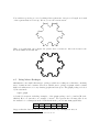
EXERCISE 25
6.3
Create the following picture:
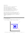
Clipping
Clipping is a process to select just those parts of a picture that lie inside an area that is
determined by a cyclic path and to discard the portion outside this is area. The command to
do this in METAPOST is
clip picture variable to path expression;
You can use it to shade a picture element:
37
beginfig(1);
pair p[]; path c[];
c0 = -500*dir(40) -- 500*dir(40);
for i=0 upto 25:
draw c0 shifted (0,10*i);
draw c0 shifted (0,-10*i);
endfor;
p1 = (100,0);
c1 = (-20,0) -- (120,0);
c2 = p1--(100,infinity);
c3 = (-20,220){dir(-45)}..(120,140){right};
c4 = (0,0)--(0,infinity);
c5 = buildcycle(c1,c2,c3,c4);
clip currentpicture to c5;
p3 = c4 intersectionpoint c3;
p2 = (100, ypart p3);
draw (0,0)--p1--p2--p3--cycle;
draw c1; draw c3 withpen pencircle scaled 2;
endfig;
end;
6.4
Dealing with Paths Parametrically
In METAPOST, a path is a continuous curve that is composed of a chain of segments. Each
segment is a cubic Bézier curve, which is determined by 4 control points. The points on the
curved segment from points p0 to p1 with post control point c0 and pre control point c1 are
determined by the formula
p(t) = (1 − t)3 p0 + 3t(1 − t)2 c0 + 3t2 (1 − t)c1 + t3 p1 ,
where t ∈ [0, 1]. If the path consists of two arcs, i.e., consists of three points p0 , p1 , and p2 ,
then the time parameter t runs from 0 to 2. If the path consists of n curve segments, then t
runs normally from 0 to n. At t = 0 it starts at point p0 and at intermediate time t = 1 the
second point p1 is reached; a third point p2 in the path, if present, is reached at t = 2, and
so on. You can get the point on a path at any time t with the construction
point t of path;
For a cyclic path with n arcs through the points p0 , p1 , . . . , pn−1 , the normal parameter range
is 0 ≤ t < n, but point t of path can be computed for any t by first reducing t modulo n.
The number of arcs in a path is available through
length(path);
The correspondence between the time parameter and a point on the curve is also used to
create a subpath of the curve. The command has the following syntax
subpath pair expression of path expression;
38
If the value of the pair expression is (t1,t2) and the path expression equals p, then the
result is a path that follows p from point t1 of p to point t2 of p. If t1 > t2, then the
subpath runs backward along p.
Based on the subpath operation are the binary operators cutbefore and cutafter. For
intersecting paths p1 and p2,
p1 cutbefore p2;
is equivalent to
subpath(xpart(p1 intersectiontimes p2), length(p1)) of p1;
except that it also sets the path variable cuttings to the parts of p1 that gets cut off. With
multiple intersections, it tries to cut off as little as possible. Similarly,
p1 cutafter p2;
tries to cut off the part of p1 after its last intersection with p2.
We have seen that for a time parameter t we can find the corresponding point on the curve
p by the statement point t of p; Another statement, of the general form
direction t of path;
allows you to obtain a direction vector at the point of the path that corresponds with time t.
The magnitude of the direction vector is somewhat arbitrary. The directiontime operation
is the inverse of the direction of operation. Given a direction vector (a pair) and a path,
directiontime direction vector of path;
return a numeric value that gives the first time t when the path has the indicated direction.
directionpoint direction vector of path;
returns the first point on the path where the given direction is achieved.
The more familiar concept of arc length is also provided for in METAPOST:
arclength(path);
returns the arc length of the given path. If p is a path and a is a number between 0 and
arclength(p), then
arctime a of p;
gives the time t such that
arclength(subpath(0,t) of p) = a;
A summary of the path operators is listed in the table below:
39
Name
arclength
arctime of
Arguments and
left
right
–
path
numeric path
Result
result
numeric
numeric
cutafter
path
path
path
cutbefore
path
path
path
direction of
directionpoint of
directiontime of
intersectionpoint
intersectiontimes
numeric
pair
pair
path
path
path
path
path
path
path
path
pair
numeric
pair
numeric
length
point of
subpath
–
numeric
pair
path
path
path
numeric
pair
path
Meaning
arc length of a path.
time on a path where arc length
from the start reaches a given value.
left argument with part after the
intersection dropped.
left argument with part before the
intersection dropped.
the direction of a path at a given time.
point where a path has a given direction.
time when a path has a given direction.
an intersection point.
times (t1 , t2 ) on paths p1 and p2
when the paths intersect.
number of arcs in a path.
point on a path given a time value.
portion of a path for given range of
time values times.
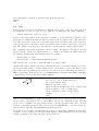
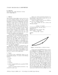
Let us apply what we have learned in this subsection to a couple of examples. In the first
example, we draw a tangent line at a point of a curve.
Ti
Ui
Ti−1
beginfig(1);
path c;
c = (0,0){dir(60)}..(100,50){dir(10)};
pair p[];
p0 = point(0.1) of c;
p1 = point(0.5) of c;
p2 = point(0.9) of c;
p3 = direction(0.5) of c;
dotlabel.lrt(btex $T_{i-1}$ etex, p0);
dotlabel.lrt(btex $U_i$ etex, p1);
dotlabel.lrt(btex $T_i$ etex, p2);
draw c;
draw (-p3 -- p3) scaled (40/xpart(p3))
shifted p1;
endfig;
end;
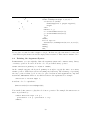
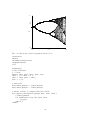
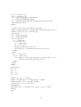
The second example is the trefoil knot, i.e, the torusknot of type (1,3). The METAPOST code
has been written such that assigning n = 5 and n = 7 draws the torusknot of type (1,5) and
(1,7), respectively, in a nice way.
beginfig(1);
pair A,B; path p[];
numeric n; n:=3;
40
A = (0,2cm); B = A rotated (2*360/n);
p0 = A{dir(180)}..tension((n+1)/2)..
B{dir(180+2*360/n)};
numeric a;
(a,whatever) = p0 intersectiontimes
(p0 rotated (360/n));
p1 = subpath(0,a-.04) of p0;
p2 = subpath(a+.04,1) of p0;
drawoptions(withpen pencircle scaled 2);
for i=0 upto n-1:
draw p1 rotated (i*360/n);
draw p2 rotated (i*360/n);
endfor;
endfig;
end;
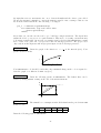
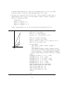
The third example shows a few steps in the Newton iterative method of finding zeros.
y
O
x2
x1
x0
x
beginfig(1);
u := 1cm;
draw (-.5u,0)--(5u,0);
draw (0,-.5u)..(0,4u);
label.llft(btex $O$ etex, (0,0));
label.rt(btex $x$ etex, (5u,0));
label.top(btex $y$ etex, (0,4u));
path f;
f = (.25u,-.5u){right}..(5u,4u){dir(70)};
draw f withpen pencircle scaled 1.2pt;
x0 = 4.6*u;
numeric t[];
for i=0 upto 1:
(t[i],whatever) = f intersectiontimes
((x[i],-infinity)--(x[i],infinity));
z[i] = point t[i] of f;
(x[i+1],0) = z[i] +
whatever*direction t[i] of f;
draw (x[i],0)--z[i]--(x[i+1],0);
fill fullcircle scaled 3.6pt shifted z[i];
endfor;
label.bot(btex $x_0$ etex, (x0,0));
label.bot(btex $x_1$ etex, (x1,0));
label.bot(btex $x_2$ etex, (x2,0));
endfig;
end;
41
EXERCISE 26
Create the following picture, which has to do with Kepler’s law of areas.
∆t0
∆t
Sun
7
Control Structures
In this section we shall look at two commonly used control structures of imperative programming languages, viz., condition and repetition.
7.1
Conditional Operations
The basic form of a conditional statement is
if condition: balanced tokens else: balanced tokens fi
where condition represents an expression that evaluates to a boolean value (i.e., true or false)
and the balanced tokens normally represent any valid METAPOST statement or sequence of
statements separated by semicolons. The if statement is used for branching: depending on
some condition, one sequence of METAPOST statements is executed or another. The keyword
fi is the reverse of if and marks the end of the conditional statement. The keyword fi
separates the statement sequence of the preceding command clause so that the semicolon at
the end of the last command in the else: part can be omitted. It also marks the end of the
conditional statement so that you do not need a semicolon after the keyword to separate the
conditional statement from then next statement.
Other forms of conditional statements are obtained from the basic form by:
• Omitting the else: part when there is nothing to be said.
• Nesting of conditional operations. The following shortcut can be used: else: if can be
replaced by elseif, in which case the corresponding fi must be omitted. For example,
nesting of two basic if operations looks as follows:
if 1st condition: 1st tokens elseif 2nd condition: 2nd tokens fi
Let us give an example: computing the center of gravity (also called barycenter) of a number
of objects with randomly generated weight and position. The example contains many more
programming constructs, some of which will be covered in sections later on in the tutorial;
so you may ignore them if you wish. The nested conditional statement is easily found in the
METAPOST code below. With the commands numeric(x) and pair(x) we test whether x is
a number or a point, respectively.
42
2.22429
1.37593 0.48659
0.68236
1.39641
0.73831
1.0579 0.00526
beginfig(1);
vardef centerofgravity(text t) =
save x, wght, G, X;
pair G,X; numeric wght, w;
G := origin; wght:=0;
for x=t:
if numeric(x):
show("weight = "& decimal(x));
G:= G + x*X;
wght := wght + x;
elseif pair(x):
show("location = (" &
decimal(xpart(x)) & ", " &
decimal(ypart(x)) & ")");
X:=x; % store pair
else:
errmessage("should not happen");
fi;
endfor;
G/wght
enddef;
numeric w[]; pair A[];
n:=8;
for i=1 upto n:
A[i] = 1.5cm*
(normaldeviate, normaldeviate);
w[i] = abs(normaldeviate);
dotlabel.bot(decimal(w[i]), A[i]);
endfor;
draw centerofgravity(A[1],w[1]
for i=2 upto n: ,A[i],w[i] endfor)
withpen pencircle scaled 4bp
withcolor 0.7white;
endfig;
end;
The errmessage command is for displaying an error message if something goes wrong and
interrupting the program at this point. The show statement is used here for debugging
purposes. When you run the METAPOST program from a shell, show puts its results on the
standard output device. In our example, the shell window looked like:
(heck@remote 1) mpost barycenter
This is MetaPost, Version 0.641 (Web2C 7.3.1)
(barycenter.mp
>> "location = (-13.14597, -80.09227)"
43
>> "weight = 1.0579"
>> "location = (-19.7488, -43.93861)"
>> "weight = 1.39641"
>> "location = (-43.89838, 7.07126)"
>> "weight = 1.37593"
>> "location = (-2.69252, 9.70473)"
>> "weight = 0.48659"
>> "location = (-24.17944, 25.14096)"
>> "weight = 2.22429"
>> "location = (-67.98569, -55.73247)"
>> "weight = 0.73831"
>> "location = (20.28859, -76.48691)"
>> "weight = 0.00526"
>> "location = (-67.07672, -18.69904)"
>> "weight = 0.68236" [1] )
1 output file written: barycenter.1
Transcript written on barycenter.log.
(heck@remote 2)
The boolean expression that forms the condition can be built up with the following relational
and logical operators.
Relational Operators
Operator Meaning
=
equal
<>
unequal
<
less than
<=
less than or equal
>
greater than
>=
greater than or equal
Operator
and
or
not
Logical Operators
Meaning
test if all conditions hold
test if one of many conditions hold
negation of condition
One final remark on the use of semicolons in the conditional statement. Where the colons after
the if and else part are obligatory, semicolons are optional, dependinging on the context.
For example, the statement
if cycle(p): fill p;
elseif path(p): draw p;
else: errmessage("what?");
fi;
44
fills or draws a path depending on the path p being cyclic or not. You may omit whatever
semicolon in this example and rewrite it even as
if cycle(p): fill p
elseif path(p): draw p
else: errmessage("what?")
fi
However, when you use the conditional clause to build up a single statement, then you must
be more careful with placing or omitting semicolons. In
draw p withcolor if cycle(p): red else: blue fi withpen pensquare;
you cannot add semicolons after the color specifications, nor omit the final semicolon that
marks the end of the statement (unless it is a statement that is recognized as finished because
of another keyword, e.g., endfor).
7.2
Repetition
Numerous examples in previous section have used the for loop of the form
for counter = start step stepsize until finish :
loop text
endfor;
where counter is a counting variable with initial value start. The counter is incremented at
each step in the repetition by the value of stepsize until it passes the value of finish. Then
the repetition stops and METAPOST continues with what comes after the endfor part. The
loop text is usually any valid METAPOST statement or sequence of statements separated by
semicolons that are executed at each step in the repetition. Instead of step 1 until, we can
also use the keyword upto. downto is another word for step -1 until. This counted for
loop is an example of an unconditional repetition, in which a predetermined set of actions are
carried out. Below, we give another example of a counted for loop: generating a Bernoulli
walk. We use the normaldeviate operator to generate a random number with the standard
normal distribution (mean 0 and standard deviation 1).
beginfig(1);
n := 60; pair p[]; p0 = (0,0);
for i=1 upto n:
p[i] = p[i-1] +
(3,if normaldeviate>0: -3 else: 3 fi);
endfor;
draw p0 for i=1 upto n: --p[i] endfor;
endfig;
end;
The last example in the previous section, in which we computed the center of gravity of
randomly generated weighted points, contained another unconditional repetition, viz., the
for loop over a sequence of zero or more expressions separated by commas. Another example
of this kind is:
45
(80,120)
(20,100)
(0,0)
(40,0)
beginfig(1);
fill for p=(0,0),(40,0),(80,120),(20,100):
p-- endfor cycle withcolor 0.8white;
for p=(0,0),(40,0),(80,120),(20,100):
dotlabel.bot("(" & decimal(xpart(p)) &
"," & decimal(ypart(p)) & ")", p);
endfor;
endfig;
end;
Nesting of counted for loops is of course possible, but there are no abbreviations: balancing
with respect to for and endfor is obligatory. You must use both endfor keywords in
for i=0 upto 10:
for j=0 upto 10:
show("i = " & decimal(i) & ", j = " & decimal(j));
endfor
endfor
EXERCISE 27
Create the following picture:
EXERCISE 28
Create the picture below, which illustrates the upper and lower Riemann
sum for the area enclosed by the horizontal axis and the graph of the function f (x) = 4 − x2 .
46
EXERCISE 29
Create the following piece of millimeter paper.
EXERCISE 30
A graph is bipartite when its vertices can be partitioned into two disjoint
sets A and B such that each of its edges has one endpoint in A and the other in B. The most
famous bipartite graph is K3,3 show below to the left. Write a program that draws the Kn,n
graph for any natural number n > 1. Show that your program indeed creates the graph K5,5 ,
which is shown below to the right.
a5
b5
a4
b4
a3
b3
a3
b3
a2
b2
a2
b2
a1
b1
a1
b1
Another popular type of repetition is the conditional loop. METAPOST does not have a preor post conditional loop (while loop or until loop) built in. You must create one by an
endless loop and an explicit jump outside this loop. First the endless loop: this is created by
forever: loop text endfor;
To terminate such a loop when a boolean condition becomes true, use an exit clause:
exitif boolean expression;
When the exit clause is encountered, METAPOST evaluates the boolean expression and exits
the current loop if the expression is true. Thus, METAPOST’s version of a until loop is
forever:
loop text;
exitif boolean expression;
endfor;
If it is more convenient to exit the loop when an expression becomes false, then use the
predefined macro exitunless Thus, METAPOST’s version of a while loop is:
forever: exitunless boolean expression;
loop text
endfor
47
8
8.1
Macros
Defining Macros
In the section about the repetition control structure we introduced upto as a shortcut of
step 1 until. This is also how it is is internally defined in METAPOST:
def upto = step 1 until enddef;
It is a definition of the form
def name = replacement text enddef;
It calls for a macro substitution of the simplest kind: subsequent occurrences of the token
name will be replaced by the replacement text. The name in a macro is a variable name;
the replacement text is arbitrary and may for example consist of a sequence of statements
separated by semicolons.
It is also possible to define macros with arguments, so that the replacement text can be
different for different calls of the macro. An example of a built-in, parametrized macro is:
def rotatedaround(expr z, d) =
shifted -z rotated d shifted z
enddef;
% rotates d degrees around z
Although it looks like a function call, a use of rotatedaround expands into in-line code.
The expr in this definition means that a formal parameter (here z or d) can be an arbitrary
expression. Each occurrence of a formal parameter will be replaced by the corresponding
actual argument (this is referred to as ‘call-by-value’). Thus the line
rotatedaround(p+q, a+b);
will be replaced by the line
shifted -(p+q) rotated (a+b) shifted (p+q);
Macro parameters need not always be expressions. Another argument type is text, indicating
that the parameters are just past as an arbitrary sequence of tokens.
8.2
Grouping and Local Variables
In METAPOST, all variables are global by default. But you may want to use in some piece of
METAPOST code a variable that has temporarily inside that portion of code a value different
from the one outside the program block. The general form of a program block is
begingroup statements endgroup
where statements is a sequence of one or more statements separated by semicolons. For
example, the following piece of code
x := 1; y := 2;
begingroup x:=3; y:=x+1; show(x,y); endgroup
show(x,y);
48
will reveal that the x and y values are 3 and 4, respectively, inside the program block. But
right after this program block, the values will be as before, viz., 1 and 2.
The program block is used in the definition of the hide macro:
def hide(text t) = exitif numeric begingroup t; endgroup; enddef;
It takes a text parameter and interprets it as a sequence of statements while ultimately
producing an empty replacement text. In other words, this command allows you to run code
silently.
Grouping often occurs automatically in METAPOST. For example, the beginfig macro starts
with begingroup and the replacement text for endfig ends with endgroup. vardef macros
are always grouped automatically, too.
You may want to go one step further: not only treating values of a variable locally, but also its
name. For example, in a macro definition you may want to use a so-called local variable, i.e.,
a variable that only has meaning inside that definition and does not interfere with existing
variables. In general, variables are made local by the statement
save name sequence;
For example, the macro whatever has the replacement text8
begingroup save ?; ? endgroup
This macro returns an unknown. If the save statement is used outside of a group, the
original values are simply discarded. This explains the following definition of the built-in
macro clearxy:
def clearxy = save x,y enddef
8.3
Vardef Definitions
Sometimes we want to return a value from a macro, as if it is a function or subroutine. In
this case we want to make sure that the calculations inside the macro do not interfere with
the expected use of the macro. This is the main purpose of the vardef definition of the form
def name = replacement text; returned text enddef;
By using vardef instead of def we hide the replacement text but the last statement, which
returns a value. Below we given an example of a macro that generates a random point in
the region [l,r]×[b,u]. We use the uniformdeviate to generate a random number with
the uniform distribution between 0 and the given argument. A validity test on the actual
arguments is carried out; in case a region is not defined properly, we use errmessage to
display some text and exit from the macro call, returning the origin as default point when
computing is continued.
8
in fact, save is a vardef macro, which has the begingroup and begingroup automatically placed around
the replacement text. Thus, the begingroup and endgroup are superfluous here.
49
beginfig(1);
vardef randompoint(expr l,r,b,u) =
if (r<=l) or (u<=b):
errmessage("not a proper region");
origin
else:
numeric x, y;
x = l+uniformdeviate(r-l);
y = b+uniformdeviate(u-b);
(x,y)
fi
enddef;
for i=0 upto 10:
dotlabel("",randompoint(10,100,10,100));
endfor;
endfig;
end;
Do not place a semicolon after origin or (x,y). In that case, the statement becomes part
of the hidden replacement text and an empty value is returned. This causes a runtime error.
8.4
Defining the Argument Syntax
In METAPOST, you can explicitly define the argument syntax and construct unary, binary,
or tertiary operators. Let us look at the code of a predefined unary operator:
vardef unitvector primary z = z/abs z enddef;
As the example suggests, the keyword primary is enough to specify the macro as a unary
vardef operator. Other keywords are secondary and tertiary. The advantage of specifying
an n-ary operator is that you do not need to place brackets around arguments in compound
statements; METAPOST will sort out which tokens are the arguments. For example
unitvector v rotated angle v;
is understood to be equivalent to
(unitvector(v)) rotated(angle(v));
You can also define a macro to play the role of an of operation. For example, the direction of
macro is predefined by
vardef direction expr t of p =
postcontrol t of p - precontrol t of p
enddef;
50
8.5
Precedence Rules of Binary Operators
METAPOST provides the classifiers primarydef, secondarydef, and tertiarydef (for def
macros, not for vardef macros) to set the level of priority of a binary operator. In the
example below, the orthogonal projection of a vector v along another vector w is defined as a
secondary binary operator.
u1
u4
2u2
u3
8.6
u2
beginfig(1);
secondarydef v projectedalong w =
if pair(v) and pair(w):
(v dotprod w) / (w dotprod w) * w
else:
errmessage "arguments must be vectors"
fi
enddef;
pair u[]; u1 = (20,80); u2 = (60,15);
drawarrow origin--u1;
drawarrow origin--u2;
drawarrow origin--2*u2;
u3 = u1 projectedalong u2;
u4 = 2*u2 projectedalong u1;
drawarrow origin--u3 withcolor blue;
draw u1--u3 dashed withdots;
draw ((1,0)--(1,1)--(0,1))
zscaled (6pt*unitvector(u2)) shifted u3;
drawarrow origin--u4 withcolor blue;
draw 2*u2--u4 dashed withdots;
draw ((1,0)--(1,1)--(0,1))
zscaled (6pt*unitvector(-u1)) shifted u4;
labeloffset := 4pt;
label.rt(btex $u_1$ etex, u1);
label.bot(btex $u_2$ etex, u2);
label.bot(btex $2u_2$ etex, 2*u2);
label.bot(btex $u_3$ etex, u3);
label.lft(btex $u_4$ etex, u4);
endfig;
end;
Recursion
A macro is defined recursively if in its definition, it makes a call to itself. Recursive definition
of a macro is possible in METAPOST. We shall illustrate this with the computation of a
Pythagorean tree.
51
beginfig(1)
u:=1cm; branchrotation := 60;
offset := 180-branchrotation;
thinning := 0.7;
shortening := 0.8;
def drawit(expr p, linethickness) =
draw p withpen pencircle scaled linethickness;
enddef;
vardef tree(expr A,B,n,size) =
save C,D,thickness; pair C,D;
thickness := size;
C := shortening[B, A rotatedaround(B,
offset+uniformdeviate(branchrotation))];
D := shortening[B, A rotatedaround(B,
-offset-uniformdeviate(branchrotation))];
if n>0:
drawit(A--B, thickness);
thickness := thinning*thickness;
tree(B, C, n-1, thickness);
tree(B, D, n-1, thickness);
else:
drawit(A--B,thickness);
thickness := thinning*thickness;
drawit(B--C, thickness);
drawit(B--D, thickness);
fi;
enddef;
tree((0,0), (0,u), 10, 2mm);
endfig;
end;
EXERCISE 31
The Koch snowflake is constructed as follows: start with an equilateral
triangle. Break each edge into four straight pieces by adding a bump a shown below.
52
You can then repeat the process of breaking a line segment into four pieces of length one-fourth
of the segment that is broken up. Below you see the next iteration.
Write a program that can compute the picture after n iterations. After six iteration, the
Koch snowflake should like like
8.7
Using Macro Packages
METAPOST comes with built-in macro packages, which are nothing more than files containing
macro definitions and constants. The most valuable macro package is graph, which contains
high-level utility macros for easy drawing graphs and data plots. The graph package is loaded
by the statement
input graph
A detailed description, including examples, of the graph package can be found in [Hob92b,
GRS94]. Here, we just show one example of its use. We represent the following data about
the annual beer consumption in the Netherlands in the period 1980–2000 graphically9 .
year
liter
1980
86
1985
85
1990
91
1995
86
2000
83
Suppose that the data are stored columnwise in a file, say consumption.dat, as
9
Compare this example with your own code in exercise 22.
53
1980
1985
1990
1995
2000
86
85
91
86
83
The following piece of code produces a line plot of the data. The only drawback of the
graph package appears: years are by default marked by decade. This explains the erroneous
horizontal labels.
86
input graph;
beginfig(1);
draw begingraph(4cm,4cm);
gdraw "consumption.dat";
endgraph;
endfig;
84
end;
90
88
1980 1990 1990 2000 2000
A few changes in the code draws the data point as bullets, changes the frame style, limits the
number of tick marks on the horizontal axis, and puts labels near the axes.
consumption in liters
•
90
88
86
•
•
•
84
•
1980
1990
year
2000
beginfig(1);
draw begingraph(4cm,4cm);
gdraw "consumption.dat" plot btex $\bullet$ etex;
Gmarks := 3; % limit number of ticks
frame.llft;
glabel.lft(btex consumption in liters etex
rotated 90, OUT);
glabel.bot(btex year etex, OUT);
endgraph;
endfig;
end;
With the graph package, you can easily change in a plot the ticks, the scales, the grid used
an/or displayed, the title of the plot, and so on.
8.8
Mathematical functions
The following METAPOST code defines some mathematical functions that are not built-in.
Note that METAPOST contains two trigonometric functions, viz., sind and cosd, but they
expect their argument in degrees, not in radians.
vardef sqr
vardef log
primary x = (x*x)
enddef;
primary x = (if x=0: 0 else: mlog(x)/mlog(10) fi) enddef;
54
vardef ln
primary x = (if x=0: 0 else: mlog(x)/256 fi)
enddef;
vardef exp primary x = ((mexp 256)**x)
enddef;
vardef inv primary x = (if x=0: 0 else: x**-1 fi)
enddef;
vardef pow (expr x,p) = (x**p)
enddef;
% trigonometric functions
numeric pi; pi := 3.1415926;
numeric radian; radian := 180/pi; % 2pi*radian = 360 ;
vardef tand
primary x = (sind(x)/cosd(x))
enddef;
vardef cotd
primary x = (cosd(x)/sind(x))
enddef;
vardef sin
primary x = (sind(x*radian))
enddef;
vardef cos
primary x = (cosd(x*radian))
enddef;
vardef tan
primary x = (sin(x)/cos(x))
enddef;
vardef cot
primary x = (cos(x)/sin(x))
enddef;
% hyperbolic functions
vardef sinh
primary x = save xx ; xx = exp xx ; (xx-1/xx)/2 enddef ;
vardef cosh
primary x = save xx ; xx = exp xx ; (xx+1/xx)/2 enddef ;
vardef tanh
primary x = (sinh(x)/cosh(x))
enddef;
vardef coth
primary x = (cosh(x)/sinh(x))
enddef;
% inverse trigonometric and hyperbolic functions
vardef arcsind primary x = angle((1+-+x,x))
enddef;
vardef arccosd primary x = angle((x,1+-+x))
enddef;
vardef arcsin
primary x = ((arcsind(x))/radian) enddef;
vardef arccos
primary x = ((arccosd(x))/radian) enddef;
vardef arccosh primary x = ln(x+(x+-+1))
enddef;
vardef arcsinh primary x = ln(x+(x++1))
enddef;
Most definitions speak for themselves, except that you may not be familiar with Pythagorean
addition (++) and substraction (+-+):
p
p
++(a, b) = a2 + b2 , + − +(a, b) = a2 − b2 .
9
More Examples
The examples in this section are meant to give you an idea of the strength of METAPOST.
9.1
Electronic Circuits
mpcirc is a macro package for drawing electronic circuits, developed by Tomasz Cholewo and
downloadable from http://ci.uofl.edu/tom/software/LaTeX/mpcirc/. Let us use it to
create some diagrams. We show the diagrams and the code to create them. The basic idea
of mpcirc is that you have at your disposal a set of predefined electronic components such as
resistor, capacity, diode, and so on. Each component has some connection points, referred to
by a, b, . . ., for wires. You place the elements, using predefined orientations, and then connect
them with wires. This mode of operating with mpcirc is referred to as turtle-based. Another
programming style for drawing diagrams is node-based. In this approach, the node locations
are determined first and then the elements are put between them using betw.x macros. We
shall use the turtle-mode in our examples and hope that the comments speak for themselves.
55
L
C
u:=10bp; % unit of length
input mpcirc;
beginfig(1);
prepare(L,C,Vac); % mention your elements
z0=(10u,10u); % lower right node
ht:=6u;
% height of circuit
z1=z0+(0,ht); % upper right node
C=.5[z0,z1];
% location of capacitor
L.t=T.r;
% use default orientation
C.t=Vac.t=T.u; % components rotated 90 degrees
% set the distance between Voltage and Capacitor
equally_spaced(5u,0) Vac, C;
L=z1-0.5(C-Vac); % location of spool
edraw; % draw components of the circuit
% draw wires connecting components
% the first ones rotated 90 degrees
wire.v(Vac.a,z0);
wire.v(Vac.b,L.a);
wire.v(L.b,z1);
wire(C.a,z0);
wire(C.b,z1);
endfig;
end;
R
L
u:=10bp; % unit of length
input mpcirc;
beginfig(1);
prepare (L,R,C,Vac); % mention your elements
z0=(0,0);
% lower left node
ht:=6u;
% height of circuit
z1=z0+(0,ht); % upper left node
56
C
Vac=.5[z0,z1]; % location of voltage
Vac.t=T.u;
% rotated 90 degrees
L.t=R.t=C.t=T.r; % default orientation
% set equal distances
equally_spaced(5u,0) z1,R,L,C,z2;
edraw; % draw elements of circuits
% draw wires connecting nodes
% the first ones rotated 90 degrees
wire.v(Vac.a,z0);
wire.v(Vac.b,z1);
wire.v(z2,z0);
wire(z1,R.a);
wire(R.b,L.a);
wire(L.b,C.a);
wire(C.b,z2);
endfig;
end;
R
L
C
u:=10bp; % unit of length
input mpcirc;
beginfig(1);
prepare (L,R,C,Vac); % mention your elements
z0=(0,0);
% lower left node
ht:=6u;
% height of circuit
z1=z0+(0,ht); % upper left node
Vac=.5[z0,z1]; % location of voltage
Vac.t=T.u;
% rotated 90 degrees
L.t=R.t=C.t=T.r; % default orientation
% set equal distances
equally_spaced(7.5u,0) z1,z2,z3;
L=0.5[z1,z2]; % location of spool
C=0.5[z2,z3]-(0,2u);
R=0.5[z2,z3]+(0,2u);
z4 = z3+(2.5u,0);
edraw; % draw elements of circuits
% draw wires connecting nodes
wire.v(Vac.a,z0);
wire.v(Vac.b,z1);
57
wire(z1,L.a);
wire(L.b,z2);
wire.v(z2,C.a);
wire.v(z2,R.a);
wire.v(z3,C.b);
wire.v(z3,R.b);
wire(z3,z4);
wire.v(z4,z0);
endfig;
end;
9.2
Marking Angles and Lines
In geometric pictures, line segments of equal length are often marked by an equal number
of ticks and equal angles are often marked the same, too. In the following example, the
macros tick, mark_angle, and mark_right_angle mark lines and angles. When dealing
with angles, we use the macro turningnumber to find the direction of a cyclic path: 1 means
counter-clockwise, -1 means clockwise. We use it to make our macros mark_angle, and
mark_right_angle independent of the order in which the non-common points of the angle
are specified.
C
A
D
B
% set some user-adjustable constants
angle_radius := 4mm;
angle_delta := 0.5mm;
mark_size := 2mm;
def mark_angle(expr A, common, B, n) = % draw 1, 2, 3 or 4 arcs
draw_angle(A, common, B, angle_radius);
if n>1: draw_angle(A, common, B, angle_radius+angle_delta); fi;
if n>2: draw_angle(A, common, B, angle_radius-angle_delta); fi;
if n>3: draw_angle(A, common, B, angle_radius+2*angle_delta); fi;
enddef;
def draw_angle(expr endofa, common, endofb, r) =
begingroup
58
save tn; tn := turningnumber(common--endofa--endofb--cycle);
draw (unitvector(endofa-common){(endofa-common)
rotated(tn*90)} .. unitvector(endofb-common)) scaled r shifted common;
endgroup
enddef;
def mark_right_angle(expr endofa, common, endofb) =
begingroup
save tn; tn :=
turningnumber(common--endofa--endofb--cycle);
draw ((1,0)--(1,1)--(0,1)) zscaled(mark_size*
unitvector((1+tn)*endofa+(1-tn)*endofb-2*common)) shifted common;
endgroup
enddef;
def tick(expr p, n) =
begingroup
save midpnt;
midpnt = 0.5*arclength(p); % find the time when half-way the path
for i=-(n-1)/2 upto (n-1)/2:
draw_mark(p, midpnt+mark_size*i/2); % place n tick marks
endfor;
endgroup
enddef;
def draw_mark(expr p, m) =
begingroup
save t, dm; pair dm;
t = arctime m of p;
% find a vector orthogonal to p at time t
dm = mark_size*unitvector(direction t of p rotated 90);
draw(-1/2dm..1/2dm) shifted (point t of p); % draw tick mark
endgroup
enddef;
beginfig(1);
pair A, B, C, D;
A := (0,0); B := (3cm,0); C := (1.5cm,4cm); D := (1.5cm,0);
draw A--B--C--cycle; draw C--D; % draw triangle and altitude
label.bot("A", A); label.bot("B", B); label.top("C", C); label.bot("D", D);
tick(A--D,1); tick(D--B,1); tick(A--C,2); tick(B--C,2);
mark_angle(C,A,B,2); mark_angle(A,B,C,2); mark_angle(B,C,A,1);
mark_right_angle(C,D,B);
endfig;
end;
59
9.3
Vectorfields
In the first example below we show the directional field corresponding with the ordinary
differential equation y 0 = y. For clarity, we show a vectorfield instead of a directional field
with small line segments.
y
y = ex
x
beginfig(1);
% some constants
numeric xmin, xmax, ymin, ymax, xinc, u;
xmin := -1.5; xmax := 1.5; ymin := 0; ymax := 4.5;
xinc := 0.05; u := 1cm;
% draw axes
draw (xmin-0.5,0)*u -- (xmax+0.5,0)*u;
draw (0,ymin-0.5)*u -- (0,ymax+0.5)*u;
% define f making up the ODE y’ = f(x,y). Here we take y’ = y
% with the exponential curve as solution curve
vardef f(expr x,y) = y enddef;
% define routine to compute function values
def compute_curve(suffix g)(expr xmin, xmax, xinc) =
( (xmin,g(xmin))
for x=xmin+xinc step xinc until xmax: .. (x,g(x)) endfor )
enddef;
% compute and draw exponential curve
vardef exp(expr x) = (mexp 256)**x enddef;
path p; p := compute_curve(exp, xmin, xmax, xinc) scaled u;
draw p;
60
% draw direction field
pair vec; path v;
for x=xmin step 0.5 until xmax:
for y=ymin+0.5 step 0.5 until ymax-0.5:
vec := unitvector( (1,f(x,y)) ) scaled 1/2u;
v := ((0,0)--vec) shifted -1/2vec;
drawarrow v shifted (x*u,y*u) withcolor blue;
endfor;
endfor;
% draw directions along the exponential curve
for x=-0.5 step 0.5 until xmax:
vec := unitvector( (1,f(x,exp(x))) ) scaled 1/2u;
v := ((0,0)--vec) shifted -1/2vec;
drawarrow v shifted (x*u,exp(x)*u) withcolor red;
endfor;
% draw ticks and labels
for x=round(xmin) upto xmax:
draw (x,-0.05)*u--(x,0.05)*u;
endfor;
for y=round(ymin) upto ymax:
draw (-0.05,y)*u--(0.05,y)*u;
endfor;
label.bot(btex $x$ etex, (xmax+0.5,0)*u);
label.lft(btex $y$ etex, (0,ymax+0.5)*u);
label(btex $y=e^x$ etex, (xmax, exp(xmax)+0.5)*u);
endfig;
end;
Now we shall show some other examples of directional fields corresponding with ODEs and solution curves using the macro package courbe from Jean-Michel Sarlat, which we downloaded
from http://melusine.eu.org/syracuse/metapost/courbes/.
y
+1
+1
(x + x2 )y 0 − y = −1
61
x
verbatimtex
%&latex
\documentclass{article}
\begin{document}
etex
input courbes;
vardef fx(expr t) = t enddef;
vardef fy(expr t) = 1+a*t/(1+t) enddef;
beginfig(1);
repere(10cm,10cm,5cm,5cm,2cm,2cm);
trace.axes(0.5pt);
marque.unites(1mm);
%% Champs de vecteurs
vardef F(expr x,y) = (y-1)/(x+x**2) enddef;
champ.vecteurs(0.1,0.1,0.2,0.15,0.5white);
%% Courbes intgrales
color la_couleur;
la_couleur = (0.9,0.1,0.9);
for n = 0 upto 20:
a := (n/8) - 1.25;
draw ftrace(-0.995,2.5,50) en_place withcolor la_couleur;
draw ftrace(-2.5,-1.1,50) en_place withcolor la_couleur;
endfor;
%
draw rpoint(r_xmin,1)--rpoint(r_xmax,1) withcolor la_couleur;
decoupe.repere;
etiquette.axes;
etiquette.unites;
label(btex $(x+x^2)y’-y=-1$ etex scaled 2.5,rpoint(0,-3));
endfig;
end;
In the next example, we added a macro to the courbes.mp package for drawing a directional
field with line segments instead of arrows.
verbatimtex
%&latex
\documentclass{article}
\begin{document}
etex
input courbes;
% ======================================== fonctions
vardef fx(expr t) = t enddef;
vardef fy(expr t) = tan(t+a) enddef;
62
% ======================================== figure
beginfig(1);
repere(10cm,10cm,5cm,5cm,2cm,2cm);
trace.axes(0.5pt);
marque.unites(1mm);
%% Champs de directions
vardef F(expr x,y) = 1+y**2 enddef;
champ.segments(0,0,0.2,0.1,0.5white);
%% Courbes intgrales
for n = 0 upto 16:
a := (n/2) - 4;
draw ftrace(-1.5-a,1.5-a,50) en_place withcolor (0.5,0.6,0.1);
endfor;
decoupe.repere;
etiquette.axes;
etiquette.unites;
label(btex $y’=1+y^2$ etex scaled 2.5,rpoint(0,-3));
endfig;
end;
y
+1
+1
x
y0 = 1 + y2
9.4
Riemann Sums
Another example of the courbes.mp macro package is the following illustration of Riemann
sums. We show two pictures for different number of segments.
63
y
y
Riemann Sum
Riemann Sum
f (ξi )
y = f (x)
f (ξi )
a
x0
xi−1
xi
b
xn
a
x0
x
ξi
S=
n
X
y = f (x)
f (ξi )(xi − xi−1 )
xi−1xi
ξi
S=
i=1
n
X
f (ξi )(xi − xi−1 )
i=1
verbatimtex
%&latex
\documentclass{article}
\everymath{\displaystyle}
\begin{document}
etex
input courbes;
vardef fx(expr t) = t enddef;
vardef fy(expr t) = (t-5)*sin(t)-cos(t)+2 enddef;
beginfig(1);
numeric a,b,n,h;
a = 1; b = 7; n = 6; h = (b-a)/n;
color aubergine; aubergine = (37/256,2/256,29/256);
repere(10cm,10cm,2cm,3cm,1cm,1cm);
fill ((a,0)--ftrace(a,b,200)--(b,0)--cycle) en_place withcolor 0.7red;
for i=1 upto n:
path cc;
aa := a + (i-1) * h;
bb := aa + h;
ff := fy(aa + h/2);
cc := rpoint(aa,0)--rpoint(aa,ff)--rpoint(bb,ff)--rpoint(bb,0);
fill cc--cycle withcolor 0.8white;
draw cc;
endfor;
trace.axes(0.5pt);
trace.courbe(a,b,200,2pt,aubergine);
64
b
xn
x
decoupe.repere;
etiquette.axes;
label.bot(btex $x_{i-1}$ etex, rpoint(a+n/2*h,0));
label.bot(btex $x_{0}$ etex, rpoint(a,0));
label.bot(btex $x_{n}$ etex, rpoint(b,0));
label.ulft(btex $\mathbf{a}$ etex, rpoint(a,0));
label.urt(btex $\mathbf{b}$ etex, rpoint(b,0));
label.top(btex $\mathbf{y=f(x)}$ etex, f(b) en_place);
label.bot(btex $x_{i}$ etex, rpoint(a+n/2*h+h,0));
projection.axes(f(a+(n+1)/2*h),0.5pt,2);
label.lft(btex $f(\xi_i)$ etex, rpoint(0,fy(a+(n+1)/2*h)));
label.bot(btex $\xi_i$ etex,rpoint(a+(n+1)/2*h,-0.4));
drawarrow rpoint(a+(n+1)/2*h,-0.4)--rpoint(a+(n+1)/2*h,-0.1);
label(btex \textit{Riemann Sum} etex scaled 2,rpoint(4,5));
label(btex $S = \sum_{i=1}^n f(\xi_i)(x_i - x_{i-1})$ etex
scaled 1.5,rpoint(5,-2));
endfig;
end;
9.5
Iterated Functions
The following diagrams are ‘standard’ in the theory of iterative processes:
• The cobweb-graph of applying the cosine function iteratively.
1
0.5
0.5
1
• The bifurcation diagram of the logistic function, i.e., of f (x) = rx(1 − x) for 0 < r < 4.
65
orbit
1
0.5
0
2.9
3.4
The code that produced these diagrams is shown below.
verbatimtex
%&latex
\documentclass{article}
\begin{document}
etex
beginfig(1)
% some constants
u := 10cm;
numeric xmin, xmax, ymin, ymax, xinc;
xmin := 0.5; xmax := 1.0;
ymin := xmin; ymax := xmax;
xinc := 0.02;
% draw axes
draw (xmin,ymin)*u -- (xmax,ymin)*u;
draw (xmin,ymin)*u -- (xmin,ymax)*u;
% define routine to compute function values
def compute_curve(suffix g)(expr xmin, xmax, xinc) =
( (xmin,g(xmin))
for x=xmin+xinc step xinc until xmax:
.. (x,g(x))
endfor )
enddef;
66
r
3.9
% compute and draw cosine curve
numeric pi; pi := 3.1415926;
numeric radian; radian := 180/pi; % 2pi*radian = 360 ;
vardef cos primary x = (cosd(x*radian)) enddef;
path p;
p := compute_curve(cos, xmin, xmax, xinc) scaled u;
draw p;
% draw identity graph
draw (xmin,ymin)*u -- (xmax,xmax)*u withcolor 0.5white;
% compute the orbit starting from some point
numeric x, initial, orbitlength;
x := 1.0; % the starting point
initial := 1; % some initial iterations
orbitlength := 15; % number of iterations
for i=1 upto initial: % do initial iterations
x := cos(x);
endfor;
dotlabel("", (x,cos(x))*u); % mark starting point
for i=1 upto orbitlength: % draw hooks
draw (x,cos(x))*u -- (cos(x),cos(x))*u -- (cos(x),cos(cos(x)))*u withcolor blue;
x := cos(x); % next value
endfor;
% draw axis labels
labeloffset := 0.25cm;
label.bot(decimal(xmin),
label.bot(decimal(xmax),
label.lft(decimal(ymin),
label.lft(decimal(ymax),
endfig;
(xmin,ymin)*u);
(xmax,ymin)*u);
(xmin,ymin)*u);
(xmin,ymax)*u);
beginfig(2)
numeric rmin, rmax, r, dr, n, ux, uy;
rmin := 2.9; rmax := 3.9;
r := rmin; n := 175;
dr := (rmax - rmin)/n;
ux := 8cm; uy := 8cm;
for i = 1 upto n:
x := 0.5; % our starting point
for j=1 upto 75: % initial iterations
x := r*x*(1-x);
endfor
for j=1 upto 150: % the next 100 iterations
x := r*x*(1-x);
draw (r*ux,x*uy) withpen pencircle scaled .5pt;
endfor
67
r := r+dr;
endfor;
% draw axes and labels
draw (rmin*ux,0) -- (rmax*ux,0);
draw (rmin*ux,0) -- (rmin*ux,uy);
labeloffset := 0.25cm;
label.bot(decimal(rmin), (rmin*ux,0));
label.bot(decimal((rmin+rmax)/2), ((rmin+rmax)/2*ux,0));
label.bot(decimal(rmax), (rmax*ux,0));
label.lft(decimal(0), (rmin*ux,0));
label.lft(decimal(0.5), (rmin*ux,0.5*uy));
label.lft(decimal(1), (rmin*ux,uy));
label.bot(btex $r$ etex, ((rmax-0.2)*ux,0));
label.lft(btex orbit etex rotated 90, (rmin*ux,0.75*uy));
endfig;
end;
9.6
A Surface Plot
You can draw surface plots from basic principles. We give one example.
Z
Y
X
z = cos(xy)
verbatimtex
%&latex
\documentclass{article}
68
\begin{document}
etex
% u: dimensional unit
% xp, yp, zp: coordinates of light source
% bf : brightness factor
% base_color : base color
numeric u,xp,yp,zp,bf;
color base_color;
u = 1cm;
xp := 3; yp := 3; zp := 5;
bf := 30;
base_color := red+green;
% O, Xr, Yr, Zr : reference frame
pair O,Xr,Yr,Zr;
O = (0,0);
Xr = (-.7,-.7) scaled u;
Yr = (1,0) scaled u;
Zr = (0,1) scaled u;
% for drawing the reference frame
vardef frameXYZ(expr s) =
drawarrow O--Xr scaled s;
drawarrow O--Yr scaled s;
drawarrow O--Zr scaled s;
label.llft(btex $X$ etex scaled 1.25, (Xr scaled s));
label.rt(btex $Y$ etex scaled 1.25, (Yr scaled s));
label.top(btex $Z$ etex scaled 1.25, (Zr scaled s));
enddef;
% from 3D to 2D coordinates
vardef project(expr x,y,z) = x*Xr + y*Yr + z*Zr enddef;
% numerical derivatives by central differences
vardef diffx(suffix f)(expr x,y) =
numeric h; h := 0.01;
(f(x+h,y)-f(x-h,y))/(2*h)
enddef;
vardef diffy(suffix f)(expr x,y) =
numeric h; h := 0.01;
(f(x,y+h)-f(x,y-h))/(2*h)
enddef;
% Compute brightness factor at a point
vardef brightnessfactor(suffix f)(expr x,y,z) =
numeric dfx,dfy,ca,cb,cc;
69
dfx := diffx(f,x,y);
dfy := diffy(f,x,y);
ca := (zp-z)-dfy*(yp-y)-dfx*(xp-x);
cb := sqrt(1+dfx*dfx+dfy*dfy);
cc := sqrt((z-zp)*(z-zp)+(y-yp)*(y-yp)+(x-xp)*(x-xp));
bf*ca/(cb*cc*cc*cc)
enddef;
% compute the colors and draw the patches
vardef z_surface(suffix f)(expr xmin,xmax,ymin,ymax,nx,ny) =
numeric dx,dy,xt,yt,zt,factor[][];
pair Z[][];
dx := (xmax-xmin)/nx;
dy := (ymax-ymin)/ny;
for i=0 upto nx:
xt := xmin+i*dx;
for j=0 upto ny:
yt := ymin+j*dy;
zt := f(xt,yt);
Z[i][j] = project(xt,yt,zt);
factor[i][j] := brightnessfactor(f,xt,yt,zt);
endfor
endfor
for i = 0 upto nx-1:
for j= 0 upto ny-1:
fill Z[i][j]--Z[i][j+1]--Z[i+1][j+1]--Z[i+1][j]--cycle
withcolor factor[i][j]*base_color;
endfor
endfor
enddef;
beginfig(1);
xp := 3;
yp := 3;
zp := 10;
bf := 100;
numeric pi; pi := 3.14159;
vardef cos primary x = cosd(x/pi*180) enddef;
vardef f(expr x,y) = cos(x*y) enddef;
z_surface(f,-3,3,-3,3,100,100);
frameXYZ(5);
label(btex $z = \cos(xy)$ etex scaled 1.25,(0,-4cm));
endfig;
end;
70
9.7
Miscellaneous
We adopt another example from Jean-Michel Sarlat that uses his macro package courbe and
another one called grille. The example has been downloaded and slightly adapted from
http://melusine.eu.org/syracuse/metapost/cours/sarlat/derivation/.
y
f 0 (a)
f (x) − f (a)
x−a
f (x)
f (a)
A
graph of f
a
x
Derivative at a point
verbatimtex
%&latex
\documentclass{article}
\begin{document}
etex
input courbes;
input grille;
vardef droite(expr a,b,t) =
(t[a,b])--(t[b,a])
enddef;
path c,cartouche;
c=(2.3cm,1cm)..(4.5cm,4cm)..(9cm,3cm);
cartouche = (3cm,2mm)--(7cm,2mm)--(7cm,8mm)--(3cm,8mm)--cycle;
pair A,M;
A = point 0.6 of c;
M = point 1.5 of c;
vardef tangente(expr t,x) =
pair X,Y;
X := point (t-.05) of c;
Y := point (t+.05) of c;
droite(X,Y,x)
enddef;
71
x
beginfig(1);
grille(1cm,0,10cm,0,7cm);
repere(10cm,7cm,2cm,2cm,1cm,1cm);
trace.axes(.5pt);
marque.unites(0.1);
%% lectures sur la grille
numeric xa,ya,xm,ym;
xa = 1.25; ya = 1.1 ; xm = 4.9 ; ym = 2.25;
pair AA,MM;
AA = (xa,ya) ; MM = (xm,ym) ;
projection.axes(AA,0.5,1.7);
projection.axes(MM,0.5,1.7);
label.bot(btex $a$ etex,rpoint(xa,0));
label.bot(btex $x$ etex,rpoint(xm,0));
label.lft(btex $f(a)$ etex, rpoint(0,ya));
label.lft(btex $f(x)$ etex, rpoint(0,ym));
%% fin des lectures
draw c withpen pencircle scaled 1.5pt withcolor (.2,.4,.9);
draw droite(A,M,1.2);
draw tangente(0.6,9) withpen pencircle scaled 1.5pt;
dotlabel.ulft(btex $A$ etex scaled 1.5,A);
dotlabel("",M);
label(btex $\displaystyle\frac{f(x)-f(a)}{x-a}$ etex scaled 1.25,
M shifted (1cm,1cm));
label.ulft(btex $f’(a)$ etex scaled 1.25, (5cm,5cm));
label.bot(btex graph of $f$ etex scaled 1.25, point 2 of c);
%% Cartouche
fill cartouche withcolor .8white;
draw cartouche;
label.rt(btex \textbf{Derivative at a point} etex,(3cm,5mm));
%% fin du cartouche
decoupe.repere;
etiquette.axes;
endfig;
end;
72
10
Solutions to the Exercises
EXERCISE 3
beginfig(1);
draw fullcircle scaled 2cm;
endfig;
end;
EXERCISE 4
beginfig(1);
path p;
p := (0,0)--(2cm,0)--(1cm,sqrt(3)*cm)--(0,0);
draw p;
endfig;
beginfig(2);
draw p scaled 1.5;
endfig;
end;
EXERCISE 5
beginfig(1);
u := 0.5cm;
draw (2u,0)--(u,sqrt(3)*u)--(-u,sqrt(3)*u)--(-2u,0)
--(-u,-sqrt(3)*u)--(u,-sqrt(3)*u)--(2u,0);
endfig;
end;
EXERCISE 6
beginfig(1);
u=1cm;
draw (0,0)--(2*sqrt(3)*u,0)--(sqrt(3)*u,3u)--(0,0);
draw (0,0)--(sqrt(3)*u,u)--(2*sqrt(3)*u,0);
draw (sqrt(3)*u,u)--(sqrt(3)*u,3u);
endfig;
beginfig(2);
draw unitsquare scaled 2u shifted (-u,-u);
draw unitsquare scaled 4u shifted (-2u,-2u);
draw (u,u)--(2u,2u);
draw (-u,u)--(-2u,2u);
draw (-u,-u)--(-2u,-2u);
draw (u,-u)--(2u,-2u);
endfig;
end;
73
EXERCISE 7
warningcheck := 0;
numeric p, q, n;
n := 12;
p := 2**n;
q := 2**n+1;
show p,q;
end;
EXERCISE 9
beginfig(1)
draw unitsquare scaled 70;
draw (10,20);
draw (10,15) scaled 2;
draw (30,40) withpen pencircle scaled 4;
pickup pencircle scaled 8;
draw (40,50);
draw (50,60);
endfig;
end;
EXERCISE 10
beginfig(1)
pickup pencircle scaled 6bp;
z.P = (1cm,2cm);
draw z.P;
draw 2(x.P,y.P);
endfig;
end;
EXERCISE 11
pair A,B,C,A’,B’,C’;
u := 1cm;
A=(0,0);
B=(5u,0);
C=(2u,3u);
A’=1/2[B,C];
B’=1/2[A,C];
C’=1/2[A,B];
beginfig(1)
draw A--B--C--A;
draw A--A’;
draw B--B’;
draw C--C’;
endfig;
beginfig(2)
draw A--B--C--A;
74
draw A--A’;
draw B--B’;
draw C--C’;
dotlabel.lft("A",A);
dotlabel.urt("B",B);
dotlabel.top("C",C);
dotlabel.urt("A’",A’);
dotlabel.ulft("B’",B’);
dotlabel.bot("C’",C’);
endfig;
beginfig(3)
pair G;
G = whatever[A,A’] = whatever[B,B’];
draw A--B--C--A;
draw A--A’;
draw B--B’;
draw C--C’;
dotlabel.lft("A",A);
dotlabel.urt("B",B);
dotlabel.top("C",C);
dotlabel.urt("A’",A’);
dotlabel.ulft("B’",B’);
dotlabel.bot("C’",C’);
dotlabel.llft("",G);
label.llft("G",G-(0,1.5mm));
endfig;
end;
EXERCISE 12
beginfig(1)
s := 2cm;
z0 = s*dir(0);
z1 = s*dir(72);
z2 = s*dir(2*72);
z3 = s*dir(3*72);
z4 = s*dir(4*72);
draw z0--z1--z2--z3--z4--z0;
endfig;
end;
EXERCISE 13
beginfig(1);
z = (1cm,1cm);
draw z withpen pencircle scaled 6;
z1 = z - 2cm*dir(135);
z2 = z + 2cm*dir(135);
z3 = z + 2cm*dir(105);
draw z1--z2;
draw z--z3;
endfig;
end;
75
EXERCISE 14
pair p[];
p0 = (0,0);
p1 = (2cm,3cm);
p2 = (3cm,2cm);
beginfig(1);
fill p0--p1--p2--p0;
endfig;
beginfig(2);
fill p0--p1--p2--cycle withcolor 0.5white;
endfig;
end;
EXERCISE 15
beginfig(1);
draw origin--2*cm*dir(0);
draw origin--2*cm*dir(40);
drawarrow 1cm*dir(0){dir(90)}..
1cm*dir(40){dir(130)}
endfig;
end;
EXERCISE 16
beginfig(1);
u := 1cm;
z0 = origin; z1 = (2u,0);
draw z0--z1--z2;
draw z0{up}...z2;
draw z2{down}...z0;
pickup pencircle scaled 6;
draw z0; draw z1; draw z2;
endfig;
z2 = (u,sqrt(3)*u);
end;
EXERCISE 17
beginfig(1)
path p;
p = (0,1cm)..(1cm,0)...(0,-1cm);
fill p{dir(157)}..(0,0){dir(23)}..{dir(157)}cycle;
draw p..(-1cm,0)..cycle;
fill (0,-0.6cm)..(0.1cm,-0.5cm)..(0,-0.4cm)..(-0.1cm,-0.5cm)..cycle
withcolor white;
fill (0,0.6cm)..(0.1cm,0.5cm)..(0,0.4cm)..(-0.1cm,0.5cm)..cycle;
endfig;
end;
76
EXERCISE 18
pair A,B,C,C’;
path arc,mark[];
numeric AC, BC; % directional angle of AC and BC
u := 0.75cm; A=(0,0); B=(5u,0); C=(2u,3u);
AC = angle(A-C); BC = angle(B-C);
C’ = whatever[A,B] = C + whatever*dir(1/2*AC+1/2*BC);
arc = (C+0.5u*dir(AC)){dir(AC+90)}..{dir(BC+90)}(C+0.5u*dir(BC));
mark[1] = C+0.4u*dir(3/4*AC+1/4*BC)-C+0.6u*dir(3/4*AC+1/4*BC);
mark[2] = C+0.4u*dir(1/4*AC+3/4*BC)-C+0.6u*dir(1/4*AC+3/4*BC);
beginfig(1)
draw A--B--C--cycle; draw C--C’;
dotlabel.lft("A",A); dotlabel.urt("B",B);
dotlabel.top("C",C); dotlabel.bot("C’",C’);
draw arc; draw mark[1]; draw mark[2];
endfig;
end;
EXERCISE 19
pair A,B,C,A’,B’,C’,I;
u := 0.75cm; A=(0,0); B=(5u,-u); C=(2u,3u);
A’ = whatever[B,C] = A + whatever*dir(
1/2*angle(B-A)+1/2*angle(C-A));
B’ = whatever[A,C] = B + whatever*dir(
1/2*angle(A-B)+1/2*angle(C-B));
C’ = whatever[A,B] = C + whatever*dir(
1/2*angle(A-C)+1/2*angle(B-C));
I = whatever[A,A’]=whatever[B,B’];
beginfig(1)
draw A--B--C--cycle;
draw A--A’; draw B--B’; draw C--C’;
draw A’..B’..C’..cycle;
dotlabel.lft("A",A); dotlabel.rt("B",B);
dotlabel.top("C",C); dotlabel.urt("A’",A’);
dotlabel.ulft("B’",B’); dotlabel.bot("C’",C’);
labeloffset := 0.3cm;
dotlabel.llft("I",I);
endfig;
end;
EXERCISE 20
verbatimtex
%&latex
\documentclass{article}
\begin{document}
etex
beginfig(1)
u := 1cm;
numeric xmin, xmax, ymin, ymax, xinc;
77
xmin := 0; xmax := 4;
ymin := 0; ymax := 2;
% draw axes
draw (xmin,0)*u -- (xmax,0)*u;
draw (0,ymin)*u -- (0,ymax)*u;
% compute and draw graph of function
path p;
xinc := 0.1;
p := (xmin,sqrt(xmin))*u
for x=xmin+xinc step xinc until xmax:
.. (x,sqrt(x))*u
endfor;
draw p withpen pencircle scaled 2;
% draw tickmarks and labels
for i=0 upto xmax:
label.bot(decimal(i), (i,0)*u);
draw (i,-0.05)*u--(i,0.05)*u;
endfor;
for i=0 upto ymax:
label.lft(decimal(i), (0,i)*u);
draw (-0.05,i)*u--(0.05,i)*u;
endfor;
\labeloffset := 0.5u;
label.bot(btex $x$ etex, ((xmin+xmax)/2,0)*u);
label.lft(btex $y$ etex, (0,(ymin+ymax)/2)*u);
label(btex $y=\sqrt{x}$ etex, ((xmin+3xmax)/4,(ymin+2ymax)/3)*u);
endfig;
end;
EXERCISE 21
verbatimtex
%&latex
\documentclass{article}
\usepackage{amsmath,amssymb}
\begin{document}
etex
beginfig(1)
a := 3cm; b := 2cm;
phi := angle(a,b);
draw (-1/2cm,0)--(a+1/2cm,0); % horizontal axis
draw (0,-1/2cm)--(0,b+1/2cm); % vertical axis
draw (a,0)--(a,b)--(0,b) dashed evenly;
draw origin--(a,b);
label.llft(btex $0$ etex, (0,0));
label.bot(btex $a$ etex, (a,0));
label.lft(btex $ib$ etex, (0,b));
label.lft(btex $\mathbb{C}$ etex, (0,b+1/2cm));
label.rt(btex $a+ib=z$ etex, (a,b));
label(btex $\lbrace$ etex xscaled 1.5 yscaled 10
rotated(phi-90), 1/2(a,b) + dir(90+phi)*1.5mm);
label(btex $|z|$ etex, 1/2(a,b) + dir(90+phi)*5mm);
draw (1/2cm,0){up}..1/2cm*dir(phi){dir(90+phi)};
label(btex $\phi$ etex, 7mm*dir(phi/2));
endfig;
end;
78
EXERCISE 22
verbatimtex
%&latex
\documentclass{article}
\begin{document}
etex
beginfig(1)
u := 0.6cm;
labeloffset := 1/3u;
defaultscale := 8pt/fontsize(defaultfont);
% the data
z1 = (1980,86); z2 = (1985,85); z3 = (1990,91);
z4 = (1995,86); z5 = (2000,83);
yoff := 80; % vertical offset
% draw axes
draw (0,0)--(1/4u,0)--(1/3u,1/8u)--(5/12u,-1/8u)
--(1/2u,0)--(6u,0);
draw (0,0)--(0,1/4u)--(-1/8u,1/3u)--(1/8u,5/12u)
--(0,1/2u)--(0,6.5u);
% draw horizontal axis and data points
for i=1 upto 5:
draw (1/2+i,-1/12)*u--(1/2+i,1/12)*u; %ticks
label.bot(decimal(x[i]), ((1/2+i)*u,0)); % labels
dotlabel("", (1/2+i,(y[i]-yoff)/2)*u); % data point
endfor
% draw line graph
draw (3/2,(y[1]-yoff)/2)*u
for i=2 upto 5: --(1/2+i, (y[i]-yoff)/2)*u endfor;
% draw vertical axis
for i=1 upto 6:
draw (-1/12,i)*u--(1/12,i)*u; % ticks
label.lft(decimal(yoff+2i), (0,i*u)); % labels
endfor
% draw horizontal and vertical texts
label.bot(btex year etex, (7/2u,-1/2u));
label.lft(btex beer consumption (liter) etex
rotated 90, (-1/2u,7/2u));
endfig;
end;
EXERCISE 23
u := 1/2cm; defaultscale := 8pt/fontsize(defaultfont);
beginfig(1);
path sqr; sqr := unitsquare scaled u;
for i=0 upto 10:
label.bot(decimal(i/10), ((i+1/2)*u,0));
label.lft(decimal(i/10), (0,(i+1/2)*u));
for j=0 upto 10:
fill sqr shifted (i*u,j*u) withcolor (i*0.1+j*0.1)/3*white;
draw sqr shifted (i*u,j*u); % for drawing the grid
endfor;
endfor;
79
label.bot("r", (6u,-2/3u));
label.lft("g", (-u,6u));
label.top("RGB(r,g,0)", (6u,11u));
endfig;
beginfig(2);
path sqr; sqr := unitsquare scaled u;
for i=0 upto 10:
label.bot(decimal(i/10), ((i+1/2)*u,0));
label.lft(decimal(i/10), (0,(i+1/2)*u));
for j=0 upto 10:
fill sqr shifted (i*u,j*u) withcolor (0.3*i*0.1+0.59*j*0.1)*white;
draw sqr shifted (i*u,j*u); % for drawing the grid
endfor;
endfor;
label.bot("r", (6u,-2/3u));
label.lft("g", (-u,6u));
label.top("RGB(r,g,0)", (6u,11u));
endfig;
end;
EXERCISE 24
beginfig(1);
path O[], l[]; pair A[];
O1 = fullcircle xscaled 1cm yscaled 1/2cm shifted (0,1cm);
O2 = O1 rotated -120;
A1 = (-1/2cm,1cm);
A2 = A1 xscaled -1;
l1 = A1{down}..(A2 rotated -120){down rotated 60};
l2 = A2{down}..(A1 rotated -120){down rotated 60};
draw O1; draw O2; draw l1; draw l2;
endfig;
end;
EXERCISE 25
beginfig(1);
r := 3cm;
path C[], p[], a;
C1 = fullcircle scaled 2r;
C2 = fullcircle scaled (2/3*2r);
p1 = origin -- r*dir(20);
p2 = origin -- r*dir(35);
a := buildcycle(p1,C2,p2,C1);
fill a withcolor red+green;
draw a withpen pencircle scaled 1bp;
draw p1; draw p2;
endfig;
end;
80
EXERCISE 26
beginfig(1);
u := 1cm; a := 6u; b := 3.5u;
pair sun; sun := (-1.75u,0);
path E[], p[], area[];
E1 = fullcircle xscaled a yscaled b;
E2 = E1 scaled 1.1;
p1 = sun -- (5u*dir(8) shifted sun);
p2 = sun -- (4u*dir(28) shifted sun);
p3 = sun -- (2u*dir(75) shifted sun);
p4 = sun -- (1.75u*dir(150) shifted sun);
area1 = buildcycle(p1,E1,p2);
area2 = buildcycle(p3,E1,p4);
fill area1 withcolor red+green;
fill area2 withcolor red+green;
draw p1; draw p2; draw p3; draw p4; draw E1;
draw (-a/2,0)--(a/2,0) dashed withdots;
draw sun withpen pencircle scaled 6bp;
label.bot(btex Sun etex, sun);
numeric t[]; % intersection times
t1 = ypart (p1 intersectiontimes E2);
t2 = ypart (p2 intersectiontimes E2);
t3 = ypart (p3 intersectiontimes E2);
t4 = ypart (p4 intersectiontimes E2);
drawarrow subpath (t1,t2) of E2;
drawarrow subpath (t3,t4) of E2;
label.urt(btex $\Delta t$ etex, point((t1+t2)/2) of E2);
label.ulft(btex $\Delta t’$ etex, point((t3+t4)/2) of E2);
endfig;
end;
EXERCISE 27
beginfig(1);
u:=1cm;
draw (-2u,0)--(2u,0);
draw (0,-2u)--(0,2u);
for i=-2u step u until 2u:
draw (i,u/10)--(i,-u/10);
draw (u/10,i)--(-u/10,i);
endfor;
for i=-2u step u/5 until 2u:
draw (i,u/20)--(i,-u/20);
draw (u/20,i)--(-u/20,i);
endfor;
endfig;
end;
EXERCISE 28
beginfig(1);
u:=1cm;
numeric xmin, xmax, ymin, ymax;
81
xmin := -2.1; xmax := 2.1;
ymin := -0.5; ymax := 4.5;
% draw axes
path xaxis, yaxis;
xaxis = (xmin,0)*u -- (xmax,0)*u;
yaxis = (0,ymin)*u -- (0,ymax)*u;
% compute the graph of f
def f(expr x) = (4-x**2) enddef;
inc := 0.01;
path pts_f;
pts_f := (xmin*u,f(xmin)*u)
for x=xmin+inc step inc until xmax:
.. (x*u,f(x)*u)
endfor;
% compute and draw rectangles
n := 12; % number of rectangles
x0 := -2; x1 := 2;
inc := (x1-x0)/n;
for i=x0 step inc until x1-inc:
path p;
p = (i,0)--(i+inc,0)--(i+inc,max(f(i),f(i+inc)))
--(i, max(f(i),f(i+inc)))--cycle;
p := p scaled u;
fill p withcolor red+green;
draw p;
endfor;
draw pts_f withpen pencircle scaled 2;
draw xaxis;
draw yaxis;
pair t; % translation vector
t := (6u,0);
for i=x0 step inc until x1-inc:
path p;
p = (i,0)--(i+inc,0)--(i+inc,min(f(i),f(i+inc)))
--(i, min(f(i),f(i+inc)))--cycle;
p := p scaled u shifted t;
fill p withcolor red+green;
draw p;
endfor;
draw pts_f shifted t withpen pencircle scaled 2;
draw xaxis shifted t;
draw yaxis shifted t;
endfig;
end;
EXERCISE 29
beginfig(1)
u:=1cm;
draw (-2u,0)--(2u,0);
draw (0,-2u)--(0,2u);
for i=-2u step u until 2u:
draw(i,2u)--(i,-2u);
draw (2u,i)--(-2u,i);
endfor;
for i=-2u step u/10 until 2u:
82
draw (i,2u)--(i,-2u) withpen pencircle scaled .1bp;
draw (2u,i)--(-2u,i) withpen pencircle scaled .1bp;
endfor;
endfig;
end;
EXERCISE 30
beginfig(1)
u:=1cm;
pair A[], B[];
n := 3;
for i=1 upto n:
A[i] = (0,i*u);
B[i] = (n/2*u,i*u);
endfor;
for i=1 upto n:
for j=1 upto n:
draw A[i]--B[j];
endfor;
endfor
for i=1 upto n:
dotlabel.lft("a" & decimal(i), A[i]);
dotlabel.rt("b" & decimal(i), B[i]);
endfor;
endfig;
end;
EXERCISE 31
u:=3cm;
vardef koch(expr A,B,n) =
save C; pair C;
C = A rotatedaround(1/3[A,B], 120);
if n>1:
koch( A,
1/3[A,B], n-1);
koch( 1/3[A,B], C,
n-1);
koch( C,
2/3[A,B], n-1);
koch( 2/3[A,B], B,
n-1);
else:
draw A--1/3[A,B]--C--2/3[A,B]--B;
fi;
enddef;
beginfig(1)
z0=(u,0);
z1=z0 rotated 120;
z2=z1 rotated 120;
draw z0--z1--z2--cycle shifted (-3u,0);
drawarrow (-1.75u,0)--(-1.25u,0);
koch( z0, z1, 1);
koch( z1, z2, 1);
koch( z2, z0, 1);
endfig;
83
beginfig(2)
z0=(u,0);
z1=z0 rotated
z2=z1 rotated
koch( z0, z1,
koch( z1, z2,
koch( z2, z0,
endfig;
beginfig(3)
z0=(u,0);
z1=z0 rotated
z2=z1 rotated
koch( z0, z1,
koch( z1, z2,
koch( z2, z0,
endfig;
120;
120;
2);
2);
2);
120;
120;
6);
6);
6);
end;
References
[GRS94] Michel Goossens, Sebastian Rahtz, Frank Mittelbach. The LATEX Graphics Companion, Addison-Wesley (1994), ISBN 0-201-85469-4.
[Hag02]
Hans Hagen. The Metafun Manual, 2002. downloadable as
www.pragma-ade.com/general/manuals/metafun-p.pdf
[Hob92a] John D. Hobby: A User’s manual for MetaPost, AT&T Bell Laboratories Computing Science Technical Report 162, 1992.
[Hob92b] John D. Hobby: Drawing Graphs with MetaPost, AT&T Bell Laboratories Computing Science Technical Report 164, 1992.
11
Appendix
In this appendix we list the tables from the reference manual [Hob92a]. They summarize
the built-in features of METAPOST and the features defined in the boxes macro package.
Features that depend on boxes are marked by ‡ symbols. Features from plain METAPOST
are marked by † symbols.
84
A User’s Manual for MetaPost
64
Table 3: Internal variables with numeric values
Name
†ahangle
†ahlength
†bboxmargin
charcode
‡circmargin
day
‡defaultdx
‡defaultdy
†defaultpen
†defaultscale
†labeloffset
linecap
linejoin
miterlimit
month
pausing
prologues
showstopping
time
tracingcapsules
tracingchoices
tracingcommands
tracingequations
tracinglostchars
tracingmacros
tracingonline
tracingoutput
tracingrestores
tracingspecs
tracingstats
tracingtitles
truecorners
warningcheck
year
Page
37
37
22
41
58
–
55
55
39
20
19
35
35
35
–
–
22
–
–
61
61
61
62
62
62
12
62
62
62
62
–
23
12
–
Explanation
angle for arrowheads in degrees (default: 45)
size of arrowheads (default: 4bp)
extra space allowed by bbox (default 2bp)
the number of the next character to be output
clearance around contents of a circular or oval box
the current day of the month
usual horizontal space around box contents (default 3bp)
usual vertical space around box contents (default 3bp)
numeric index used by pickup to select default pen
font scale factor for label strings (default 1)
offset distance for labels (default 3bp)
0 for butt, 1 for round, 2 for square
0 for mitered, 1 for round, 2 for beveled
controls miter length as in PostScript
the current month (e.g, 3 ≡ March)
> 0 to display lines on the terminal before they are read
> 0 to output conforming PostScript using built-in fonts
> 0 to stop after each show command
the number of minutes past midnight when this job started
> 0 to show capsules too
> 0 to show the control points chosen for paths
> 0 to show commands and operations as they are performed
> 0 to show each variable when it becomes known
> 0 to show characters that aren’t infont
> 0 to show macros before they are expanded
> 0 to show long diagnostics on the terminal
> 0 to show digitized edges as they are output
> 0 to show when a variable or internal is restored
> 0 to show path subdivision when using a polygonal a pen
> 0 to show memory usage at end of job
> 0 to show titles online when they appear
> 0 to make llcorner etc. ignore setbounds
controls error message when variable value is large
the current year (e.g., 1992)
A User’s Manual for MetaPost
65
Table 4: Other Predefined Variables
Name
†background
†currentpen
†currentpicture
†cuttings
†defaultfont
†extra beginfig
†extra endfig
Type
color
pen
picture
path
string
string
string
Page
25
40
40
28
19
81
81
Explanation
Color for unfill and undraw (usually white)
Last pen picked up (for use by the draw command)
Accumulate results of draw and fill commands
subpath cut off by last cutbefore or cutafter
Font used by label commands for typesetting strings
Commands for beginfig to scan
Commands for endfig to scan
A User’s Manual for MetaPost
66
Table 5: Predefined Constants
Name
†beveled
†black
†blue
†bp
†butt
†cc
†cm
†dd
†ditto
†down
†epsilon
†evenly
false
†fullcircle
†green
†halfcircle
†identity
†in
†infinity
†left
†mitered
†mm
nullpicture
†origin
†pc
pencircle
†pensquare
†pt
†quartercircle
†red
†right
†rounded
Type
numeric
color
color
numeric
numeric
numeric
numeric
numeric
string
pair
numeric
picture
boolean
path
color
path
transform
numeric
numeric
pair
numeric
numeric
picture
pair
numeric
pen
pen
numeric
path
color
pair
numeric
†squared
true
†unitsquare
†up
†white
†withdots
numeric
boolean
path
pair
color
picture
Page
35
12
12
2
35
–
2
–
–
6
–
32
13
23
12
23
31
2
28
6
35
2
14
–
–
38
39
2
–
12
6
35
35
13
–
6
12
32
Explanation
linejoin value for beveled joins [2]
Equivalent to (0,0,0)
Equivalent to (0,0,1)
One PostScript point in bp units [1]
linecap value for butt end caps [0]
One cicero in bp units [12.79213]
One centimeter in bp units [28.34645]
One didot point in bp units [1.06601]
The " character as a string of length 1
Downward direction vector (0, −1)
1
Smallest positive MetaPost number [ 65536
]
Dash pattern for equal length dashes
The boolean value false
Circle of diameter 1 centered on (0, 0)
Equivalent to (0,1,0)
Upper half of a circle of diameter 1
Identity transformation
One inch in bp units [72]
Large positive value [4095.99998]
Leftward direction (−1, 0)
linejoin value for mitered joins [0]
One millimeter in bp units [2.83464]
Empty picture
The pair (0, 0)
One pica in bp units [11.95517]
Circular pen of diameter 1
square pen of height 1 and width 1
One printer’s point in bp units [0.99626]
First quadrant of a circle of diameter 1
Equivalent to (1,0,0)
Rightward direction (1, 0)
linecap and linejoin value for round joins
and end caps [1]
linecap value for square end caps [2]
The boolean value true
The path (0,0)--(1,0)--(1,1)--(0,1)--cycle
Upward direction (0, 1)
Equivalent to (1,1,1)
Dash pattern that produces dotted lines
A User’s Manual for MetaPost
67
Table 6: Operators (Part 1)
Name
&
*
*
**
+
++
+-+
-
-
/
< = >
<= >=
<>
†abs
and
angle
arclength
arctime
of
ASCII
†bbox
Argument/result types
Left
Right
Result
string
string
string
path
path
path
numeric
color
color
numeric
numeric
pair
pair
color
numeric
color
numeric
numeric
pair
pair
numeric
numeric
numeric
color
color
color
numeric
numeric
numeric
pair
pair
pair
numeric
numeric
numeric
numeric
numeric
numeric
color
color
color
numeric
numeric
numeric
pair
pair
pair
–
color
color
numeric
numeric
pair
pair
color
numeric
color
numeric
numeric
pair
pair
string
string
boolean
numeric
numeric
pair
pair
color
color
transform transform
–
numeric
numeric
pair
boolean
boolean
boolean
–
pair
numeric
–
path
numeric
numeric
path
numeric
–
–
bluepart
boolean
bot
–
–
–
†ceiling
†center
–
–
string
picture
path
pen
color
any
numeric
pair
numeric
picture
path
pen
Page
14
Explanation
13
Concatenation—works for paths l&r if
r starts exactly where the l ends
Multiplication
13
Multiplication
13
13
Exponentiation
Addition
14
14
13
√
Pythagorean addition l2√+ r2
Pythagorean subtraction l2 − r2
Subtraction
13
Negation
13
Division
13
Comparison operators
15
Absolute value
13
15
30
30
Logical and
2−argument arctangent (in degrees)
Arc length of a path
Time on a path where arclength from
the start reaches a given value
ASCII value of first character in string
A rectangular path for the bounding
box
numeric
path
–
22
numeric
boolean
numeric
pair
numeric
pair
16
16
38
15
22
Extracts the third component
Is the expression of type boolean?
Bottom of current pen when centered
at the given coordinate(s)
Least integer greater than or equal to
Center of the bounding box
A User’s Manual for MetaPost
68
Table 7: Operators (Part 2)
Name
char
color
cosd
†cutafter
Left
–
–
–
path
Argument/result
Right
numeric
any
numeric
path
types
Result
string
boolean
numeric
path
Page
†cutbefore
path
path
path
28
cycle
decimal
†dir
†direction
of
†directionpoint of
directiontime of
†div
†dotprod
floor
fontsize
greenpart
hex
infont
†intersectionpoint
intersectiontimes
†inverse
known
length
†lft
–
–
–
numeric
path
numeric
numeric
path
boolean
string
pair
pair
15
15
6
28
pair
path
numeric
30
pair
path
numeric
28
numeric
pair
–
–
–
–
string
path
numeric
pair
numeric
string
color
string
string
path
numeric
numeric
numeric
numeric
numeric
numeric
picture
pair
–
13
15
20
16
–
22
27
path
path
pair
27
–
–
–
–
–
transform
boolean
numeric
numeric
pair
pair
31
16
28
38
llcorner
22
lrcorner
–
pair
22
Lower-left corner of bounding box
makepath
makepen
–
–
transform
any
path
numeric
pair
picture
path
pen
picture
path
pen
pen
path
Times (tl , tr ) on paths l and r
when the paths intersect
Invert a transformation
Does argument have a known value?
Number of arcs in a path
Left side of current pen when its
center is at the given coordinate(s)
Lower-left corner of bounding box
path
pen
39
39
mexp
mlog
†mod
normaldeviate
–
–
–
–
numeric
numeric
numeric
–
numeric
numeric
numeric
numeric
Cyclic path bounding the pen shape
A polygonal pen made from the
convex hull of the path knots
The function exp(x/256)
The function 256 ln(x)
The remainder function l − rbl/rc
Choose a random number with
mean 0 and standard deviation 1
22
16
15
28
–
–
–
–
Explanation
Character with a given ASCII code
Is the expression of type color?
Cosine of angle in degrees
Left argument with part after the
intersection dropped
Left argument with part before the
intersection dropped
Determines whether a path is cyclic
The decimal representation
(cos θ, sin θ) given θ in degrees
The direction of a path at a given
‘time’
Point where a path has a given
direction
‘Time’ when a path has a given
direction
Integer division bl/rc
vector dot product
Greatest integer less than or equal to
The point size of a font
Extract the second component
Interpret as a hexadecimal number
Typeset string in given font
An intersection point
A User’s Manual for MetaPost
69
Table 8: Operators (Part 3)
Name
Argument/result
Left
Right
–
boolean
–
any
–
string
–
numeric
boolean
boolean
–
any
–
any
–
any
pair
pen
types
Result
boolean
boolean
numeric
boolean
boolean
boolean
boolean
boolean
pair
Page
–
numeric
numeric
any
path
path
boolean
pair
pair
16
27
–
numeric
path
pair
–
–
color
path
numeric
path
16
37
numeric
†rt
–
scaled
picture
path
pair
pen
transform
picture
path
pair
pen
transform
–
picture
path
pair
pen
transform
–
–
picture
path
pair
pen
transform
numeric
pair
numeric
pair
picture
path
pair
pen
transform
picture
path
pair
pen
transform
numeric
picture
path
pair
pen
transform
numeric
string
30
†round
picture
path
pair
pen
transform
–
not
numeric
oct
odd
or
pair
path
pen
penoffset
of
picture
point of
postcontrol
of
precontrol
of
redpart
reverse
rotated
shifted
sind
slanted
sqrt
str
numeric
pair
numeric
pair
numeric
pair
numeric
numeric
numeric
suffix
13
16
–
–
13
16
16
16
–
–
15
38
30
Explanation
Logical negation
Is the expression of type numeric?
Interpret a string as an octal number
Is the closest integer odd or even?
Logical inclusive or
Is the expression of type pair?
Is the expression of type path?
Is the expression of type pen?
Point on the pen furthest to the
right of the given direction
Is the expression of type picture?
Point on a path given a time value
First Bézier control point on path
segment starting at the given time
Last Bézier control point on path
segment ending at the given time
Extract the first component
‘time’-reversed path with beginning
swapped with ending
Rotate counterclockwise a given
number of degrees
round each component to the nearest
integer
Right side of current pen when
centered at given coordinate(s)
Scale all coordinates by the given
amount
30
Add the given shift amount to each
pair of coordinates
15
30
Sine of an angle in degrees
Apply the slanting transformation
that maps (x, y) into (x + sy, y),
where s is the numeric argument
15
50
Square root
String representation for a suffix
A User’s Manual for MetaPost
70
Table 9: Operators (Part 4)
Name
string
subpath
of
substring
of
†top
transform
transformed
ulcorner
Left
–
pair
Argument/result
Right
any
path
string
14
–
numeric
pair
any
transform
numeric
pair
boolean
picture
path
pair
pen
transform
pair
38
–
picture
path
pair
pen
transform
–
–
†whatever
xpart
–
–
xscaled
picture
path
pair
pen
transform
–
–
–
yxpart
yypart
zscaled
16
28
string
–
–
–
yscaled
Page
pair
uniformdeviate
†unitvector
unknown
urcorner
xxpart
xypart
ypart
types
Result
boolean
path
picture
path
pair
pen
transform
–
–
picture
path
pair
pen
transform
picture
path
pen
numeric
pair
any
picture
path
pen
–
pair
transform
numeric
transform
transform
pair
transform
numeric
transform
transform
pair
16
31
Explanation
Is the expression of type string?
Portion of a path for given range
of time values
Substring bounded by given indices
Top of current pen when centered
at the given coordinate(s)
Is the argument of type transform?
Apply the given transform to all
coordinates
22
Upper-left corner of bounding box
numeric
–
pair
boolean
pair
15
16
22
Random number between zero and
the value of the argument
Rescale a vector so its length is 1
Is the value unknown?
Upper-left corner of bounding box
numeric
number
10
16
Create a new anonymous unknown
x or tx component
picture
path
pair
pen
transform
number
number
number
30
Scale all x coordinates by the
given amount
32
32
16
txx entry in transformation matrix
txy entry in transformation matrix
y or ty component
30
Scale all y coordinates by the
given amount
32
32
30
tyx entry in transformation matrix
tyy entry in transformation matrix
Rotate and scale all coordinates so
that (1, 0) is mapped into the
given pair; i.e., do complex
multiplication.
picture
path
pair
pen
transform
number
number
picture
path
pair
pen
transform
A User’s Manual for MetaPost
71
Table 10: Commands
Name
addto
clip
†cutdraw
†draw
†drawarrow
†drawdblarrow
†fill
†filldraw
interim
let
†loggingall
newinternal
†pickup
save
setbounds
shipout
show
showdependencies
showtoken
showvariable
special
†tracingall
†tracingnone
†undraw
†unfill
†unfilldraw
Page
40
40
52
3
37
37
23
37
43
–
61
18
13
42
23
41
12
61
61
61
81
61
61
37
25
37
Explanation
Low-level command for drawing and filling
Applies a clipping path to a picture
Draw with butt end caps
Draw a line or a picture
Draw a line with an arrowhead at the end
Draw a line with arrowheads at both ends
Fill inside a cyclic path
Draw a cyclic path and fill inside it
Make a local change to an internal variable
Assign one symbolic token the meaning of another
Turn on all tracing (log file only)
Declare new internal variables
Specify new pen for line drawing
Make variables local
Make a picture lie about its bounding box
Low-level command to output a figure
print out expressions symbolically
print out all unsolved equations
print an explanation of what a token is
print variables symbolically
print a string directly in the PostScript output file
Turn on all tracing
Turn off all tracing
Erase a line or a picture
Erase inside a cyclic path
Erase a cyclic path and its inside
A User’s Manual for MetaPost
72
Table 11: Function-Like Macros
Name
‡boxit
‡boxit
‡boxit
‡boxjoin
‡bpath
†buildcycle
‡circleit
‡circleit
‡circleit
†dashpattern
†decr
†dotlabel
†dotlabel
†dotlabels
‡drawboxed
Arguments
suffix, picture
suffix, string
suffix, hemptyi
equations
suffix
list of paths
suffix, picture
suffix, picture
suffix, hemptyi
on/off distances
numeric variable
suffix, picture, pair
suffix, string, pair
suffix, point numbers
list of suffixes
Result
–
–
–
–
path
path
–
–
–
picture
numeric
–
–
–
–
Page
54
57
57
55
55
25
57
57
57
34
51
19
19
19
54
‡drawboxes
†drawoptions
‡drawunboxed
‡fixpos
list of suffixes
drawing options
list of suffixes
list of suffixes
–
–
–
–
57
??
57
57
‡fixsize
†incr
†label
†label
†labels
†max
†max
†min
†min
‡pic
†thelabel
†thelabel
†z
list of suffixes
numeric variable
suffix, picture, pair
suffix, string, pair
suffix, point numbers
list of numerics
list of strings
list of numerics
list of strings
suffix
suffix, picture, pair
suffix, string, pair
suffix
–
numeric
–
–
–
numeric
string
numeric
string
picture
picture
picture
pair
57
51
18
18
19
–
–
–
–
57
19
19
17
Explanation
Define a box containing the picture
Define a box containing text
Define an empty box
Give equations for connecting boxes
A box’s bounding circle or rectangle
Build a cyclic path
Put picture in a circular box
Put a string in a circular box
Define an empty circular box
Create a pattern for dashed lines
Decrement and return new value
Mark point and draw picture nearby
Mark point and place text nearby
Mark z points with their numbers
Draw the named boxes and their
contents
Draw the named boxes
Set options for drawing commands
Draw contents of named boxes
Solve for the size and position of the
named boxes
Solve for size of named boxes
Increment and return new value
Draw picture near given point
Place text near given point
Draw z point numbers; no dots
Find the maximum
Find the lexicographically last string
Find the minimum
Find the lexicographically first string
Box contents shifted into position
Picture shifted as if to label a point
text positioned as if to label a point
The pair xhsuffixi, yhsuffixi)