Download as a PDF

A Beginner’s Guide to METAPOST
for Creating High-Quality Graphics
Troy Henderson
Stephan Hennig
April 5, 2011
Abstract
Individuals that use TEX (or any of its derivatives) to typeset their documents generally
take extra measures to ensure paramount visual quality. Such documents often contain
mathematical expressions and graphics to accompany the text. Since TEX was designed “for
the creation of beautiful books — and especially for books that contain a lot of mathematics” [4], it is clear that it is sufficient (and in fact exceptional) at dealing with mathematics
and text. TEX was not designed for creating graphics; however, certain add-on packages can
be used to create modest figures. TEX, however, is capable of including graphics created with
other utilities in a variety of formats. Because of their scalability, Encapsulated PostScript
(EPS) graphics are the most common types used. This paper introduces METAPOST and
demonstrates the fundamentals needed to generate high-quality EPS graphics for inclusion
into TEX-based documents.
1
Introduction
To accompany TEX, Knuth developed METAFONT as a method of “creating entire families of
fonts from a set of dimensional parameters and outline descriptions” [1]. Approximately ten
years later, John Hobby began work on METAPOST — “a powerful graphics language based on
Knuth’s METAFONT, but with PostScript output and facilities for including typeset text” [3].
Although several packages (e.g., PICTEX, XY-pic, and the native LATEX picture environment to
name a few) are available for creating graphics within TEX-based documents, they all rely on
TEX. Since TEX was designed to typeset text, it seems natural that an external utility should be
used to generate graphics instead. Furthermore, in the event that the graphics require typeset
text, then the utility should use TEX for this requirement. This premise is exactly the philosophy
of METAPOST.
Since METAPOST is a programming language, it accommodates data structures and flow
control, and compilation of the METAPOST source code yields EPS graphics. These features
provide an elegant method for generating graphics. Figure 1 illustrates how METAPOST can be
used programatically. The figure is generated by rotating one of the circles multiple times to
obtain the desired circular chain.1
All graphics in this tutorial (except Figure 2) are created with METAPOST, and the source code and any required
external data files for each of these graphics are embedded as file attachments in the electronic PDF version of the
article. Attachments are indicated by a paper clip icon.
1
1
Figure 1: Rotated circles
The programming language constructs of METAPOST also deliver a graceful mechanism
for creating animations without having to manually create each frame of the animation. The
primary advantage of EPS is that it can be scaled to any resolution without a loss in quality. It
can also be easily converted to raster formats, e.g. Portable Network Graphics (PNG) and Joint
Photographic Experts Group (JPEG), et al., or other vector formats including Portable Document
Format (PDF) and Scalable Vector Graphics (SVG), et al.
2 METAPOST compilation
A typical METAPOST source file consists of one or more figures. Compilation of the source file
generates an EPS graphic for each figure. These EPS graphics are self-contained (i.e., the fonts
used in labels are embedded into the graphic) provided that prologues:=3 is declared.
If foo.mp is a typical METAPOST source file, then its contents are likely of the following
form:
prologues:=3;
outputtemplate:="%j-%c.mps";
beginfig(1);
draw commands
endfig;
beginfig(2);
draw commands
endfig;
...
beginfig(n);
draw commands
endfig;
end
Executing
mpost foo.mp
2
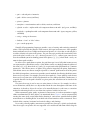
Figure 2: METAPOST Previewer
yields the following output:
This is MetaPost, Version 〈version〉
(foo.mp [1] [2] . . . [n] )
n output files written: foo-1.mps .. foo-n.mps
Transcript written on foo.log.
For users who just want to “get started” using METAPOST, a METAPOST previewer is
available at http://www.tlhiv.org/mppreview. This previewer (illustrated in Figure 2) is
simply a graphical interface to METAPOST itself. It generates a single graphic with the option
to save the output in EPS, PDF, and SVG formats. Users may also choose to save the source code
and can view the compilation log to assist in debugging.
3
Data types
3.1
Standard data types
There are ten data types in METAPOST: numeric, pair, path, transform, rgbcolor, cmykcolor,
string, boolean, picture, and pen. These data types allow users to store fragments of the graphics
for later use. We will briefly discuss each of these data types and elaborate on how they are used
in a typical METAPOST program.
numeric — numbers
3
pair — ordered pairs of numerics
path — Bézier curves (and lines)
picture — pictures
transform — transformations such as shifts, rotations, and slants
rgbcolor or color — triplets with each component between 0 and 1 (red, green, and blue)
cmykcolor — quadruplets with each component between 0 and 1 (cyan, magenta, yellow,
and black)
string — strings of characters
boolean — “true” or “false” values
pen — stroke properties
Virtually all programming languages provide a way of storing and retrieving numerical
values. This is precisely the purpose of the numeric data type in METAPOST. Since graphics
drawn with METAPOST are simply two dimensional pictures, it is clear that an ordered pair is
needed to identify each point in the picture. The pair data type provides this functionality. Each
point in the plane consists of an x (i.e., abscissa) part and a y (i.e., ordinate) part. METAPOST
uses the standard syntax for defining points in the plane, e.g., (x, y) where both x and y are
numeric data typed variables.
In order to store paths between points, the path data type is used. All paths in METAPOST
are represented as cubic Bézier curves. Cubic Bézier curves are simply parametric splines of
the form (x(t), y(t)) where both x(t) and y(t) are piecewise cubic polynomials of a common
parameter t. Since Bézier curves are splines, they pairwise interpolate the points. Furthermore,
cubic Bézier curves are diverse enough to provide a “smooth” path between all of the points
for which it interpolates. METAPOST provides several methods for affecting the Bézier curve
between a list of points. For example, piecewise linear paths (i.e., linear splines) can be drawn
between a list of points since all linear polynomials are also cubic polynomials. Furthermore, if
a specific direction for the path is desired at a given point, this constraint can be forced on the
Bézier curve.
The picture data type is used to store an entire picture for later use. For example, in order to
create animations, usually there are objects that remain the same throughout each frame of the
animation. So that these objects do not have to be manually drawn for each frame, a convenient
method for redrawing them is to store them into a picture variable for later use.
When constructing pairs, paths, or pictures in METAPOST, it is often convenient to apply
affine transformations to these objects. As mentioned above, Figure 1 can be constructed by
rotating the same circle several times before drawing it. METAPOST provides built-in affine
transformations as “building blocks” from which other transformations can be constructed. These
include shifts, rotations, horizontal and vertical scalings, and slantings.
For creating colored graphics, METAPOST provides two data types: rgbcolor and cmykcolor.
These data types correspond to the two supported color models RGB and CMYK. While using the
4
RGB color model, fractions of the primary colors red
, green
, and blue
are “additively
mixed”. Similarly, in the CMYK color model, the primary colors cyan
, magenta
, yellow
,
and black
are “subtractively mixed.” The former model is suitable for on-screen viewing
whereas the latter model is preferred in high-quality print. Both color types are ordered tuples,
(c1 , c2 , c3 ) and (c1 , c2 , c3 , c4 ), with components ci being numerics between 0 and 1. For example,
in the RGB color model, a light orange tone can be referred to as (1,.6,0)
, whereas in
the CMYK color model (0,.6,1,0)
corresponds to a clearly different orange tone. If a
particular color is to be used several times throughout a figure, it is natural to store this color
into a variable of type rgbcolor or cmykcolor.
The data type color is a convenient synonym for rgbcolor. Additionally, there are five
built-in RGB colors in METAPOST: black, white, red, green, and blue. So, the expression
.4(red+blue) refers to a dark violet
in the RGB color model and in the example above
(1,.6,0) could be replaced by red+.6green.
The most common application of string data types is reusing a particular string that is typeset
(or labeled). The boolean data type is the same as in other programming languages and is
primarily used in conditional statements for testing. Finally, the pen data type is used to affect
the actual stroke paths. The default unit of measurement in METAPOST is 1 bp = 1/72 in, and
the default thickness of all stroked paths is 0.5 bp. An example for using the pen data type may
include changing the thickness of several stroked paths. This new pen can be stored and then
referenced for drawing each of the paths.
The following code declares a variable of type numeric, one of type pair, and two string
variables:
numeric idx;
pair v;
string s, name;
Note, variables of type numeric need not necessarily be declared. A formerly undeclared
variable is automatically assumed to be numeric at first use.
3.2
Arrays
Just like many other programming languages MetaPost provides a way to access variables by
index. After the following variable declaration
pair a[];
it is possible to store points in the “array” a with numeric values as index. The console output of
a[1]
a[2]
a[3]
show
show
j :=
:= (0,1);
:= (0,5);
:= (10,20);
a[1];
a1;
2;
5
show a[j] + a[j+1];
is
>> (0,1)
>> (0,1)
>> (10,25)
Notice, the point stored at array index 1 can be referred to as a[1] as well as just a1,
omitting the brackets. The latter convenient—and often practised—notation works as long as
the index is a plain numeric value. If the index is a numeric variable or an expression, however,
the brackets have to be present, since, e.g., aj would clearly refer to an unrelated variable of
that name instead of index j of variable a.
Aside, MetaPost, as a macro language, doesn’t really provide true arrays. However, from a
user’s perspective, the MetaPost way of indexing variables perfectly looks like an array.
4
Common commands
The METAPOST manual [3] lists 26 built-in commands along with 23 function-like macros for
which pictures can be drawn and manipulated using METAPOST. We will not discuss each of
these commands here; however, we will focus on several of the most common commands and
provide examples of their usage.
4.1
The draw command
The most common command in METAPOST is the draw command. This command is used
to draw paths or pictures. In order to draw a path from z1:=(0,0) to z2:=(54,18) to
z3:=(72,72), we should first decide how we want the path to look. For example, if we
want these points to simply be connected by line segments, then we use
draw z1--z2--z3;
However, if we want a smooth path between these points, we use
draw z1..z2..z3;
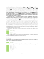
In order to specify the direction of the path at the points, we use the dir operator. In Figure 3
we see that the smooth path is horizontal at z1, a 45◦ angle at z2, and vertical at z3. These
constraints on the Bézier curve are imposed by
draw z1{right}..z2{dir 45}..{up}z3;
Notice that z2{dir 45} forces the outgoing direction at z2 to be 45◦ . This implies an
incoming direction at z2 of 45◦ . In order to require different incoming and outgoing directions,
we would use
draw z1{right}..{dir θi }z2{dir θo }..{up}z3;
6
z3
z2
z1
Figure 3: draw examples
where θi and θo are the incoming and outgoing directions, respectively.
4.2
The fill command
Another common command in METAPOST is the fill command. This is used to fill closed
paths (or cycles). In order to construct a cycle, cycle may be appended to the path declaration.
For example,
path
p :=
fill
draw
p;
z1{right}..z2{dir 45}..{up}z3--cycle;
p withcolor red;
p;
produces Figure 4. Notice that p is essentially the same curved path as in Figure 3 with the
additional piece that connects z3 back to z1 with a line segment using --cycle.
Figure 4: fill example
Just as it is necessary to fill closed paths, it may also be necessary to unfill closed paths. For
example, the annulus in Figure 5 can be constructed by
color bbblue;
bbblue := (3/5,4/5,1);
path p,q;
p := fullcircle scaled (2*54);
q := fullcircle scaled (2*27);
fill p withcolor bbblue;
unfill q;
draw p;
draw q;
7
The fullcircle path is a built-in path that closely approximates a circle in METAPOST
with diameter 1 bp traversed counter-clockwise. This path is not exactly a circle since it is
parameterized by a Bézier curve and not by trigonometric functions; however, visually it is
essentially indistinguishable from an exact circle.
Figure 5: unfill example
Notice that p is a fullcircle of radius 54 bp (3/4 in) and q is a fullcircle of radius
27 bp (3/8 in). The annulus is constructed by filling p with the baby blue color bbblue and then
unfilling q. The unfill command above is equivalent to
fill q withcolor background;
where background is a built-in color which is white by default.
Often the unfill command appears to be the natural method for constructing figures like
Figure 5. However, the fill and unfill commands in Figure 5 can be replaced by
fill p--reverse q--cycle withcolor bbblue;
p
q
Figure 6: Avoiding an unfill
The path p--reverse q--cycle travels around p in a counter-clockwise directions (since
this is the direction that p traverses) followed by a line segment to connect to q. It then traverses
clockwise around q (using the reverse operator) and finally returns to the starting point along
a line segment using --cycle. This path is illustrated in Figure 6. One reason for using
this method to construct the annulus as opposed to the unfill command is to ensure proper
transparency when placing the figure in an external document with a non-white background. If
8
the former method is used and the annulus is placed on a non-white background, say magenta,
then the result is Figure 7.
Figure 7: Improper transparency using unfill
It may be desired to have the interior of q be magenta instead of white. This could be
accomplished by redefining background; however, the latter method described above is a much
simpler solution.
4.3
Arrow commands
When drawing simple graphs and other illustrations, the use of arrows is often essential. There
are two arrow commands in METAPOST for accommodating this need — drawarrow and
drawdblarrow. Both of these commands require a path argument. For example,
drawarrow (0,0)--(72,72);
draws an arrow beginning at (0,0) and ending at (72,72) along the line segment connecting
these points.
The path argument of both drawarrow and drawdblarrow need not be line segmented
paths — they may be any METAPOST path. The only difference between drawarrow and
drawdblarrow is that drawarrow places an arrow head at the end of the path and drawdblarrow
places an arrow head at the beginning and the end of the path. As an example, to draw the
curved path in Figure 3 with an arrow head at the end of the path (i.e., at z3), the following
command can be used
drawarrow z1{right}..z2{dir 45}..{up}z3;
and is illustrated in Figure 8.
4.4
The label command
One of the nicest features of METAPOST is that it relies on TEX (or LATEX) to typeset labels within
figures. Almost all figures in technical documents are accompanied by labels which help clarify
the situation for which the figure is assisting to illustrate. Such labels may include anything from
simple typesetting as in Figures 3, 6, and 8 to typesetting function declarations and even axes
labeling.
9
z3
z2
z1
Figure 8: Using drawarrow along a path
The label command requires two arguments — a string to typeset and the point for which
label is placed. For example, the command
label("A", (0,0));
will place the letter “A” at the coordinate (0,0) and the box around this label is centered
vertically and horizontally at this point. Simple strings like "A" require no real typesetting to
ensure that they appear properly in the figure. However, many typeset strings in technical figures
require the assistance of TEX to properly display them.
y
f (x) = x2
x
Figure 9: Labeling text
For example, Figure 9 is an example where typesetting is preferred. That is, the axes labels
and the function declaration look less than perfect if TEX is not used. For reasons such as this,
METAPOST provides a way to escape to TEX in order to assist in typesetting the labels. Therefore,
instead of labeling the “A” as above,
label(btex A etex, (0,0));
provides a much nicer technique for typesetting the label. The btex ... etex block instructs
METAPOST to process everything in between btex and etex using TEX. Therefore, the function
declaration in Figure 9 is labeled using
label(btex $f(x)=x^2$ etex, (a,b));
where (a, b) is the point for which the label is to be centered.
Since many METAPOST users prefer to typeset their labels using LATEX instead of plain TEX,
METAPOST provides a convenient method for accommodating this, done in the preamble of
10
the METAPOST source file. The following code ensures that the btex ... etex block escapes
to LATEX (instead of plain TEX) for text processing.
verbatimtex
%&latex
\documentclass{minimal}
\begin{document}
etex
beginfig(n);
〈draw commands〉
endfig;
end
Often times it is desirable to typeset labels with a justification that are not necessarily
centered. For example, one may wish to place an “A” centered horizontally about (0,0), but
placed above (0,0). METAPOST provides eight suffixes to accommodate such needs. The
suffixes .lft, .rt, .bot, and .top align the label on the left, right, bottom, and top, respectively,
of the designated point. A hybrid of these four justifications provide four additional ones, namely,
.llft, .ulft, .lrt, and .urt to align the label on the lower left, upper left, lower right, and
upper right, respectively, of the designated point. For example,
label.top(btex A etex, (0,0));
places the “A” directly above (0,0). Figure 10 demonstrates each of the suffixes and their
corresponding placement of the labels.
top
lft rt
bot
ulft urt
llft lrt
Figure 10: Label suffixes
5
Graphing functions
Among the most common types of figures for TEX users are those which are the graphs of
functions of a single variable. Hobby recognized this and constructed a package to accomplish
this task. It is invoked by
input graph;
METAPOST has the ability to construct data (i.e., ordered pairs) for graphing simple
functions. However, for more complicated functions, the data should probably be constructed
using external programs such as MATLAB (or Octave), Maple, Mathematica, Gnuplot, et. al.
A typical data file, say data.d, to be used with the graph package may have contents
11
0.0
0.2
0.4
0.6
0.8
1.0
0.0
0.447214
0.632456
0.774597
0.894427
1.0
p
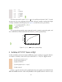
This data represents the graph of f (x) = x for six equally spaced points in [0, 1]. To graph
this data, the size of the graph must first be decided. Choosing a width of 144 bp and a height
of 89 bp, a minimally controlled plot (as in Figure 11) of this data can be generated by
draw begingraph(144bp,89bp);
gdraw "data.d";
endgraph;
The graph package provides many commands used to customize generated graphs, and
these commands are fully documented in the manual [2] for the graph package.
1
0.8
0.6
0.4
0.2
0
0
0.2
Figure 11: f (x) =
p
0.4
0.6
0.8
1
x using the graph package
Including METAPOST figures in LATEX
6
In order to include a METAPOST figure in LATEX, the graphicx package is suggested. Below is
an example of including a METAPOST figure (with name foo-1.mps) in a LATEX document.
\documentclass{article}
\usepackage{graphicx}
\begin{document}
...
\includegraphics{foo-1.mps}
...
\end{document}
Having a .mps file extension on the graphic allows the same graphic to be included in both
EX and PDFLATEX documents. When using PDFLATEX, the EPS graphic (with file extension .mps)
LAT
12
is converted to PDF “on the fly” using Hans Hagen’s mptopdf. This conversion is necessary since
PDFLATEX performs no PS processing.
7
Conclusion
METAPOST is an elegant programming language, and it produces beautiful graphics. The
graphics are vectorial and thus can be scaled to any resolution without degradation. There
are many advanced topics that are not discussed in this article (e.g., loops, flow control,
subpaths, intersections, etc.), and the METAPOST manual [3] is an excellent resource for these
advanced topics. However, the METAPOST manual may seem daunting for beginners. There
are many websites containing METAPOST examples, and several of these are referenced at
http://www.tug.org/metapost. Finally, we mention that Knuth uses nothing but METAPOST
for his diagrams.
References
[1] N. H. F. Beebe. Metafont. http://www.math.utah.edu/~beebe/fonts/metafont.html,
2006.
[2] J. D. Hobby. Drawing graphs with METAPOST. Technical Report 164, AT&T Bell Laboratories, Murray Hill, New Jersey, 1992. Also available at http://www.tug.org/docs/
metapost/mpgraph.pdf.
[3] J. D. Hobby. A user’s manual for METAPOST. Technical Report 162, AT&T Bell Laboratories,
Murray Hill, New Jersey, 1992. Also available at http://www.tug.org/docs/metapost/
mpman.pdf.
[4] D. E. Knuth. The TEXbook, volume A of Computers and Typesetting. Addison Wesley, Boston,
1986.
13