1
Syndex : User manual
Maxence Guesdon, Cécile Stentzel, Meriem Zidouni
January 17, 2014
Contents
1
Overview
1.1 The AAA methodology . . . . . . . . . . . . . . . . . . . . . . . . . . . . . . . . . . . . .
1.2 SynDEx distributions . . . . . . . . . . . . . . . . . . . . . . . . . . . . . . . . . . . . . .
2
2
2
2
Using the SynDEx tools
2.1 syndex-sdxconv . .
2.2 syndex . . . . . . .
2.3 syndex-durations .
2.4 syndex-adeq-gui .
3
4
.
.
.
.
.
.
.
.
.
.
.
.
.
.
.
.
.
.
.
.
.
.
.
.
.
.
.
.
.
.
.
.
.
.
.
.
.
.
.
.
.
.
.
.
.
.
.
.
.
.
.
.
.
.
.
.
.
.
.
.
.
.
.
.
.
.
.
.
.
.
.
.
.
.
.
.
.
.
.
.
.
.
.
.
.
.
.
.
.
.
.
.
.
.
.
.
.
.
.
.
.
.
.
.
.
.
.
.
.
.
.
.
.
.
.
.
.
.
.
.
.
.
.
.
.
.
.
.
.
.
.
.
.
.
.
.
.
.
.
.
3
3
4
6
6
Defining algorithms
3.1 Expressions . . . . . . . . .
3.2 Definitions . . . . . . . . . .
3.2.1 Sensors and actuators
3.2.2 Constants . . . . . .
3.2.3 Delays . . . . . . .
3.2.4 Functions . . . . . .
3.3 Conditioning . . . . . . . .
3.4 Repetitions . . . . . . . . .
3.4.1 Parallel repetition . .
3.5 Modules . . . . . . . . . . .
3.6 BNF . . . . . . . . . . . . .
.
.
.
.
.
.
.
.
.
.
.
.
.
.
.
.
.
.
.
.
.
.
.
.
.
.
.
.
.
.
.
.
.
.
.
.
.
.
.
.
.
.
.
.
.
.
.
.
.
.
.
.
.
.
.
.
.
.
.
.
.
.
.
.
.
.
.
.
.
.
.
.
.
.
.
.
.
.
.
.
.
.
.
.
.
.
.
.
.
.
.
.
.
.
.
.
.
.
.
.
.
.
.
.
.
.
.
.
.
.
.
.
.
.
.
.
.
.
.
.
.
.
.
.
.
.
.
.
.
.
.
.
.
.
.
.
.
.
.
.
.
.
.
.
.
.
.
.
.
.
.
.
.
.
.
.
.
.
.
.
.
.
.
.
.
.
.
.
.
.
.
.
.
.
.
.
.
.
.
.
.
.
.
.
.
.
.
.
.
.
.
.
.
.
.
.
.
.
.
.
.
.
.
.
.
.
.
.
.
.
.
.
.
.
.
.
.
.
.
.
.
.
.
.
.
.
.
.
.
.
.
.
.
.
.
.
.
.
.
.
.
.
.
.
.
.
.
.
.
.
.
.
.
.
.
.
.
.
.
.
.
.
.
.
.
.
.
.
.
.
.
.
.
.
.
.
.
.
.
.
.
.
.
.
.
.
.
.
.
.
.
.
.
.
.
.
.
.
.
.
.
.
.
.
.
.
.
.
.
.
.
.
.
.
.
.
.
.
.
.
.
.
.
.
.
.
.
.
.
.
.
.
.
.
.
.
.
.
.
.
.
.
.
.
.
.
.
.
.
.
.
.
.
.
.
.
.
.
.
.
.
.
.
.
.
.
.
.
.
.
.
.
.
.
7
8
8
8
8
9
9
11
12
12
14
15
.
.
.
.
16
16
17
18
18
.
.
.
.
.
.
.
.
.
.
.
.
Defining architectures
4.1 Medium types, media . .
4.2 Operator types, operators
4.3 Modules . . . . . . . . .
4.4 BNF . . . . . . . . . . .
.
.
.
.
.
.
.
.
.
.
.
.
.
.
.
.
.
.
.
.
.
.
.
.
.
.
.
.
.
.
.
.
.
.
.
.
.
.
.
.
.
.
.
.
.
.
.
.
.
.
.
.
.
.
.
.
.
.
.
.
.
.
.
.
.
.
.
.
.
.
.
.
.
.
.
.
.
.
.
.
.
.
.
.
.
.
.
.
.
.
.
.
.
.
.
.
.
.
.
.
.
.
.
.
.
.
.
.
.
.
.
.
.
.
.
.
.
.
.
.
.
.
.
.
.
.
.
.
.
.
.
.
.
.
.
.
.
.
.
.
.
.
.
.
5
Specifying durations
19
5.1 Operation durations . . . . . . . . . . . . . . . . . . . . . . . . . . . . . . . . . . . . . . . 19
5.2 Communication durations . . . . . . . . . . . . . . . . . . . . . . . . . . . . . . . . . . . . 20
6
Specifying placement constraints
21
7
Using adequation heuristics
23
1
Chapter 1
Overview
1.1
The AAA methodology
SynDEx is based on the AAA methodology (cf. [1]).
A SynDEx application is made of:
• algorithm graphs (definitions of operations that the application may execute),
• architecture graphs (definitions of multicomponents: set of interconnected processors and specific
integrated circuits).
Performing an adequation means to execute heuristics, seeking for an optimized implementation of a
given algorithm onto a given architecture.
An implementation consists in:
• distributing the algorithm onto the architecture (allocate parts of algorithm onto components),
• scheduling the algorithm onto the architecture (give a total order for the operations distributed onto a
component).
1.2
SynDEx distributions
SynDEx runs under Linux, Windows, and Mac OS X platforms but is currently delivered only for Linux 64
bits platforms.
SynDEx is written in Objective Caml. The Graphical User Interface uses the Gtk library through the
LablGtk bindings.
2
Chapter 2
Using the SynDEx tools
The SynDEx distribution comes with various tools :
• syndex-sdxconv translates SynDEx v7 files to SynDEx 8,
• syndex, the main command-line application, allowing to load all data to perform adequation and
generate code,
• syndex-durations is a command-line tool to handle duration files,
• syndex-adeq-gui is used to display the result of adequation heuristics.
2.1
syndex-sdxconv
Synopsis : syndex-sdxconv [options] <syndex v7 .sdx file>
This tool is used to convert SynDEx v7 .sdx files to the SynDEx 8 syntaxes. The tool reads the given
SynDEx v7 .sdx file and outputs algorithms, architectures and/or durations in SynDEx 8 syntax.
Options are :
--version
-I dir
--algo
--arch name
--dur
--cons
--split prefix
Print version number and exit
Add dir to the list of include directories (where to search files)
Dump algorithms on standard output (default action)
Dump architecture definition name (with types) on standard output
Dump durations on standard output
Dump constraints on standard output
Dump algorithms, architectures, durations, and constraints into files with prefix prefix
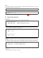
The format of algorithm files is described in section 3. The format of architecture files is described in
section 4. The format of duration files is described in section 5. The format of constraints files is described
in section 6.
Splitting the application creates several files for the architectures : one module file for all the declarations
of types and one module file for each architecture definition.
Example of a basic.arc file containing the declarations of types :
3
medium t y p e m e d i u m s a m m u l t i p o i n t : SAMMP
[ ... ]
operator type uin {
gate x : mediumsampointtopoint ;
gate y : mediumsammultipoint ;
g a t e z : mediumram ;
}
[ ... ]
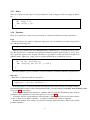
Example of a basic_ArchiSamMultiPoint.arc file containing an architecture definition :
medium medium_sammp : B a s i c . m e d i u m s a m m u l t i p o i n t
o p e r a t o r u1 : B a s i c . u i n {
y −> medium_sammp ;
}
[ ... ]
o p e r a t o r u3 : B a s i c . u o u t {
y −> medium_sammp ;
}
2.2
syndex
Synopsis : syndex [options]
Options are of two kinds : general options and action options.
The general options are :
--version
-I dir
Print version number and exit
Add dir to the list of include directories (where to search files)
The action options define actions which will be performed by syndex in the given order. Here is the list
of these actions :
4
--algo file.alg
--print-algo
--dot-algo file-alg.dot
--flatten name
--dot-flat file-flat.dot
--arch file.arc
--print-arch
--dot-arch file-arc.dot
--durations file.fd
--com-durations file.cd
--constraints file.cts
--adeq-greedy
--adeq-greedy-mp
--dot-adeq file-adeq.dot
--dump-adeq file-adeq.adq
--display-adeq
Read algorithm from file.alg
Print algorithm on standard output
Dump algorithm graph into file-alg.dot using the graphviz format
Flatten algorithm from the given definition name
Dump flat algo graph into file-flat.dot using the graphviz format
Read architecture from file.arc
Print architecture on standard output
Dump architecture graph into file-arc.dot using the graphviz format
Load operation durations from rules in file.fd
Load communication durations from rules in file.cd
Load constraints from rules in file.cts
Compute adequation with greedy heuristic
Compute multi-periodic adequation with greedy heuristic
Dump adequation result into file-adeq.dot using the graphviz format
Dump adequation result into file-adeq.adq
Display adequation
Algorithms
The syndex tool keeps a current algorithm. When launching syndex, this algorithm is empty. The --algo
option is used to add the algorithm defined in a file to the current algorithm. This option can be used several
times to add several algorithms to the current algorithm. Of course, if two loaded algorithms contain two
definitions with the same name, an error will be reported when loading the second algorithm.
The format of algorithm files is described in section 3.
Architectures
The syndex tool keeps a current architecture. When launching syndex, this architecture is empty. The
--arch option is used to add architecture declarations (declarations of types, media or operators) from a file
to the current architecture. This option can be used several times to add declarations from several files to the
current architecture. Of course, if two loaded files contain two declarations with the same name, an error
will be reported when loading the second one.
The format of architecture files is described in section 4.
Flattening
Flattening is performed with the --flatten option, giving a definition name to start the flattening from.
This definition must be given arguments if it needs. Here are some examples :
# syndex ... --flatten main ... # main requires no argument
# syndex ... --flatten "main(1)" ... # main requires one argument
# syndex ... --flatten "main(30, 12, 10)" ... # main requires three arguments
Using adequation heuristics is possible only when the algorithm has been flattened. Then, the adequation
is performed on the current flattened algorithm and the current architecture. Note that loading an additional
algorithm after the --flatten option destroys the current flattened algorithm to avoid confusion.
Adequation parameters and heuristics
Operation durations, communication durations and placement constraints are respectively loaded with
options --durations, --com-durations and --constraints.
5
The order of options matters: if an adequation was computed with an option before one of these options,
it is destroyed to avoid confusion. A message like No adequation available might appear.
The format of duration files is described in section 5 and the format of constraint files is described in
section 6.
An adequation heuristic is used with one the following options: --adeq-greedy, --adeq-greedy-mp. An
error will be reported if no flattened graph is available yet.
The result of the heuristic can be stored in a (binary) file using the --dump-adeq option.
So it is possible to perform several adequations with several parameters sequentially with one syndex
command. Here is an example of command performing twice the greedy adequation heuristic, with two
different sets of operation durations :
# syndex --algo my-algo.alg --flatten main --arch my-arch.arc \
--constraints myconstraints.cts --com-durations mycomdurs.cd \
--durations mydurs1.fd --adeq-greedy --dump-adeq adeq1.adq \
--durations mydurs2.fd --adeq-greedy --dump-adeq adeq2.adq
Binary dumps of adequation results can be viewed with the syndex-adeq-gui tool (see section 2.4) or
with the --display-adeq option. Note that you may have to modify your PATH to help syndex finding the
syndex-adeq-gui tool.
2.3
syndex-durations
Synopsis : syndex-durations [options] <files>
This tool can be used to handle (operation and communication) duration files (see section 5). The given
duration files are loaded and the result of the grouping/expanding is written on standard output.
Options are :
--version
--by-1
--by-2
--expand
2.4
Print version number and exit
Group rules by factorizing elements of first field (default)
Group rules by factorizing elements of second field
Expand all rules
syndex-adeq-gui
Synopsis : syndex-adeq-gui <file>
This tool is used to graphically display the result of an adequation heuristic, stored in the file in argument.
This file must be a binary dump produced by the --dump-adeq option of the syndex tool.
This tool provides an interactive graphical display: textual information displayed for each distributed
operation pointed with the mouse, and colors indicating predecessor and successor relations between operations.
6
Chapter 3
Defining algorithms
Algorithms are defined in .alg files, using a specific syntax.
An algorithm file contains the declarations of definitions, one after another, in precedence order, that is,
if definition d1 contains a reference to definition d2 , then d2 must appear before d1 in the algorithm file.
Remember that algorithms are composed of :
• definitions of various kinds : function, sensor, actuator, delay, constant,
• references to definitions,
• ports of references and definitions.
Definitions have ports and contain references to other definitions. If a definition d have ports, then
the reference r to d automatically has the same ports as d. We say that r references d and each port of r
references a port of d.
A definition d also have links, representing the data flow. There are various possibilities for links :
• links from an input port of d to an output port of d,
• links from an input port of d to an input port of a reference contained in d,
• links from an output port of a reference contained in d to an output port of d,
• links from an output port of a reference r1 to an input port of a reference r2 , with r1 and r2 contained
in d.
Sensor and constants can only have output ports. Actuator can only have input ports. Delays can only
have one input port and one output port.
References may have some attributes :
• a period, in case of a multi-periodic application,
• an abstract flag, indicating that the reference must be considered as a "leaf" when flattening the algorithm,
• repetition information, used to repeat references when flattening the algorithm; repetitions can be
sequential or parallel.
Ports are defined by their direction (input or output), their type and their size.
At last, definitions can have parameters. A reference to a definition having n parameters must have n
arguments.
7
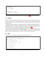
3.1
Expressions
Expressions are used to express port sizes and repetition factors. The arguments to references are expressions, too. The parameters of a definition are identifiers which are bounds to the arguments of the reference
when flattening the graph.
By now, the expressions are composed only of integer constants, variable names, binary operations (’+’,
’-’, ’*’ and ’/’) and unary negation ’-’. Parenthesis are used as usual to deambiguate expressions, and ’*’
and ’/’ have higher priority than ’+’ and ’-’.
Here are some examples of valid expressions :
• 1
• 1 +2
• (1 + 2) ∗ (− 3 − 1)
• (a + b) ∗ 3 / 1
• x
3.2
Definitions
A definition is describe using the following general syntax.
< d e f i n i t i o n k i n d > name < p a r a m e t e r s > { <body > }
The definition kind is one of the following keywords : actuator, constant, delay function, sensor.
The name is an identifier composed of any of the characters ’a’..’z’, ’A’..’Z’, ’0’..’9’, ’_’ and beginning
with a lowercase letter (’a’..’z’).
If the definition has parameters, they are indicated between parentheses and separated by commas. Each
parameter must be a valid simple identifier following the same lexical convention as definition names.
The syntax of the definition body depends on the kind of the definition.
3.2.1
Sensors and actuators
The body of sensor and actuator definitions is composed only of a list of port declarations (see below).
Examples :
sensor input1 { i n t [ 3 ] data1 , char d a t a 2 }
actuator output1 ( size ) { i n t [ size ] data }
3.2.2
Constants
The body of constant definitions is composed only of a list of declarations of ports and values. Example :
c o n s t a n t c s t { i n t o = 2 , f a c t o r = 42 }
8
3.2.3
Delays
The body of delays are only composed of port declarations, with one input port and one output port. Example :
d e l a y memory {
in : i n t [ 2 ] v_in ;
out : i n t [ 2 ] v_out ;
}
3.2.4
Functions
The body of a function is composed of port declarations, references declarations and edge declarations.
Ports
Functions can have any number of input and output ports. A port is defined by its name, its type and its
size, with the following syntax :
<type > < o p t i o n a l s i z e > <name> < o p t i o n a l e x t e n s i o n a t t r i b u t e s >
The type is any identifier but is used during flattening to check that types of connected ports are consistent. The optional size is a valid expression and must be indicated between square brackets ’[’ and ’]’. If no
size is given, the expression 1 is assumed. The name of a port must follow the same lexical conventions as
definition names. Input (resp. output) ports are specified with the in (resp. out) keyword, as in :
function foo ( a , b ) {
in : i n t bar , f l o a t [ b ] gee ;
o u t : c h a r [ a+b ] buz [ x=" 16 " , y=" 478 " ] ;
...
}
Extension attributes of ports are similar to extension attributes of references which are explained below.
References
References are introduced with the construction
l e t <reference_name > = < q u a l i f i e d _ d e f i n i t i o n _ n a m e > < o p t i o n a l
arguments > < o p t i o n a l a t t r i b u t e s > ;
A reference name is a lowercase identifier following the same lexical convention as definition names.
The qualified definition name is either a simple definition name or a name with the form Module_name.definition_name
(see section 3.5 about modules).
If the referenced definition has parameters, arguments must be given after the definition name, between
parentheses. These arguments are any valid expressions (see section 3.1).
A reference can have various attributes, indicated with a comma-separated list between square brackets
’[’ and ’]’. There are two kinds of attributes : "predefined" attributes and "extension" attributes.
Predefined attributes allow setting some properties about the defined references. Here are the existing
predefined attributes :
9
• abstract : when this attribute is specified, the reference will be considered as a final component
(a ’leaf’) of the algorithm during the flattening, which means that the flattening will not flatten the
algorithm below (the definition referenced by) this reference,
• period : this attribute, followed by an integer, indicates the period of the reference, in multi-periodic
applications,
• parallel and sequence : these attributes, followed by a repetition factor e, indicate that this reference
must be repeated e times during the flattening. e is an expression. Repetitions are explained in section
3.4.
Here is an example of reference declarations :
f u n c t i o n example ( a , b ) {
...
l e t f o o 1 = compute1 ( 1 , b ) [ a b s t r a c t , p e r i o d 3 ] ;
l e t f o o 2 = compute1 ( a , 12 ) [ p e r i o d 5 , p a r a l l e l ( a + b ) ] ;
l e t f o o 3 = compute2 ;
...
}
Extension attributes are pairs (key, value) allowing to associate any string value to any key. This will be
useful in the future to allow syndex extensions (others heuristics) to specify and use additional information
about references. Extension attributes are given with the syntax key="value" in the attribute list. Here is
an example :
f u n c t i o n example ( a , b ) {
...
l e t f o o 4 = compute1 ( a , b ) [ x=" 125 " , y=" 257 " , p e r i o d 12 ] ;
...
}
These extension attributes are used for example by graphical editors to store the coordinates of references
in graphical display of definitions.
Edges
A definition contains edges between ports to indicate data flow, and edges between references to indicate
a precedence order.
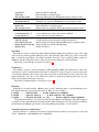
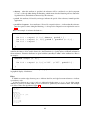
A data flow between two ports p1 and p2 is indicated with the syntax p1 -> p2 . A port of the current
definition is given by its name, while a port of a reference is qualified by the reference name. The example
code below creates the algorithm of figure 3.1.
function foo {
in : i n t i ;
out : i n t o ;
}
function bar {
in : i n t v_in ;
out : i n t v_out1 , i n t v_out2 ;
l e t r1 = foo ;
l e t r2 = foo ;
v _ i n −> r 1 . i ;
v _ i n −> r 2 . i ;
r 1 . o −> v _ o u t 1 ;
r 2 . o −> v _ o u t 2 ;
r 1 −−> r 2 ;
}
10
Figure 3.1: Algorithme with edges.
In the example above, a precedence edge from r1 to r2 (r1 --> r2) is also added to indicate that reference
r1 must be scheduled before the reference r2.
3.3
Conditioning
Conditionning is introduced by the following construction in the body of a function :
match < p o r t name> w i t h
n1 −> < r e f e r e n c e and e d g e s d e c l a r a t i o n s >
| n2 −> < r e f e r e n c e and e d g e s d e c l a r a t i o n s >
| ...
The ports of the definition must be declared before the conditioning structure. The port name must
be one of the input port of the definition. n1, n2, . . . , must be integer constants (by now). For each
case, references and edges can be added. One can add two references with the same name if they are in
two different cases. Under each case, only the ports of the definition and the references under this case
are known, so edges under each case can only concern ports of the definition and references under this
case. Nested conditions are not allowed. To represent nested conditions, one must create one definition per
condition.
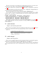
The following code defines and used a conditioned function, and figure 3.2 shows the resulting algorithm :
function switch_1 ( ) {
i n : i n t i , i n t cond ;
out : i n t o ;
match cond w i t h
| 1 −>
l e t r_mul = I n t . a r i t _ m u l ( 1 ) ;
cond −> r _ m u l . b ;
i −> r _ m u l . a ;
r _ m u l . o −> o ;
| 2 −>
l e t r_add = I n t . a r i t _ a d d ( 1 ) ;
cond −> r _ a d d . b ;
i −> r _ a d d . a ;
r _ a d d . o −> o ;
}
11
f u n c t i o n main ( ) {
l e t switch_1 = switch_1 ;
l e t input_2 = Int . input (1) ;
l e t input_1 = Int . input (1) ;
let output = Int . output (1) ;
s w i t c h _ 1 . o −> o u t p u t . i ;
i n p u t _ 2 . o −> s w i t c h _ 1 . cond ;
i n p u t _ 1 . o −> s w i t c h _ 1 . i ;
}
Figure 3.2: Algorithm with conditioning.
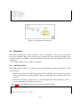
3.4
Repetitions
The specified algorithm may contain indications to repeat some references. It is a way to ease the definition of the algorithm. Indeed, these repetitions are not dynamic but static. Before the flattening of the
algorithm, repetitions are handled to obtain an algorithm as if references had been manually repeated in the
specification.
Two kinds of repetition exist : parallel or sequential.
3.4.1
Parallel repetition
The parallel repetition indicated on a reference consists in duplicating the reference and adding two additional operations :
• upstream of these references, an Explode operation allows to distribute, between the various instances
of the repeated reference, the data provided by the ports producing the data consumed by the repeated
reference,
• downstream, an Implode operation allows to collect the output data of these instances to send it to
ports consuming the data of the repeated reference.
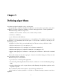
Figure 3.3 shows the flattened graph obtained from the following algorithm :
function f ( ) {
in : i n t [ 2 ] i1 , i n t i2 , i n t [ 3 ] i 3 ;
o u t : i n t [ 6 ] o1 , i n t o2 ;
}
s e n s o r c a p t e u r ( ) { i n t [ 6 ] o1 , i n t o2 , i n t [ 3 ] o3 }
actuator a c t i o n n e u r ( ) { i n t [ 6 ] i1 , i n t [ 3 ] i 2 }
12
Figure 3.3: Example of parallel repetition.
f u n c t i o n main ( ) {
let capt = capteur ;
let act = actionneur ;
l e t f = f [ p a r a l l e l 3 ( i 2 = , i 3 / , o2 ∗ , o1 / ) ] ;
c a p t . o1 −> f . i 1 ;
c a p t . o2 −> f . i 2 ;
c a p t . o3 −> f . i 3 ;
f . o1 −> a c t . i 1 ;
f . o2 −> a c t . i 2 ;
}
This example illustrates the three possible strategies to distribute the data in a parallel repetition :
• the port i of the reference f has no particular indication in the parallel repetition attribute, so it is given
the "Mul" strategy, meaning that the producers of the data feeding this port must produce N times
more data to feed all repetitions (N being the repetition factor, here N = 3). Since the size of port
i1 of f is 2, the port o1 of capteur has its size set to 2 ∗ N = 6 (by the user) to that port sizes are
consistent ; so the port i1 of Explode_f has a size of 6 and its output ports i1 has each a size of 2,
• the choice for port i3 of f is symetrical : the producers of the data feeding i3 don’t have to produce
more data, but we divide the port size of repetitions of f by N, which gives a size of 1, with consistent
sizes for the ports i3 of Explode_f ; this is the "Div" strategy,
• fort port i2 of f, we choose to send the same data to all repetitions of f, so all input and output ports i2
of Explode_f have the same size ; this is the "Equal" strategy.
The reasoning is similar for the Implode_f operation and the output ports of the repetitions of f, except that
the "Equal" strategy is not allowed because the Implode operation cannot choose which data to transmit
among all the received data (the repetitions will usually not output the same data).
Remark : The repetition does not modify the size of ports of data producers and consumers of f, bu
controls are performed to check consistency between these sizes. The user is responsible for giving correct
sizes.
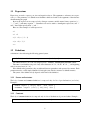
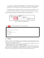
Répétition séquentielle
The sequential repetition consists in repeating a reference to create a pipeline with these repetitions. The
data source for each input port of repetitions must be indicated, with two alternatives :
• If a link is given from an output port o to an input port i (with the syntax i <- o), this means that
between two copies r1 and r2 in sequence in this order, the data from port o of r1 will feed the port
13
i of r2 . The prot i of the first reference of the pipeline will consume the data of the producer of the
original (repeated) reference in the algorithm and data or port o of the last reference of the pipeline
will feed to the ports consuming the port o of the original (repeated) reference of the algorithm,
• If a distribution strategy is indicated for an input port, this strategy is used in an Explode operation
created and feeding the corresponding ports, the samy way as for parallel repetitions (see above).
If no information is given about one input port, the "Mul" distribution strategy is used to feed this port
in each copy of the repeated reference, from that data producer of the original algorithm.
Figure 3.4: Example of sequential repetition.
Figure 3.4 show the flattened algorithm for the following algorithm :
function f ( ) {
in : i n t [ 2 ] i1 , i n t i2 , i n t [ 3 ] i 3 ;
o u t : i n t [ 6 ] o1 , i n t o2 ;
}
s e n s o r c a p t e u r ( ) { i n t [ 6 ] o1 , i n t o2 , i n t [ 3 ] o3 }
actuator a c t i o n n e u r ( ) { i n t [ 6 ] i1 , i n t [ 1 ] i 2 }
f u n c t i o n main ( ) {
let capt = capteur ;
let act = actionneur ;
l e t f = f [ s e q u e n c e 3 ( i 3 / , o2−> i 2 ) ] ;
c a p t . o1 −> f . i 1 ;
c a p t . o2 −> f . i 2 ;
c a p t . o3 −> f . i 3 ;
f . o1 −> a c t . i 1 ;
f . o2 −> a c t . i 2 ;
}
3.5
Modules
A module system allows separate definition of pieces of algorithm. A module contains definitions and can
be seen as a library. As soon as a file foo.alg contains one definition, another algorithm file can use the
module Foo to use the definitions in foo.alg.
Refering to a module definition is done simply by prefixing the definition name with the module name,
as in Int.arit_add which refers to definition arit_add of module Int.
When a module name appears, the corresponding algorithm file is looked up in the include directories
(specified by -I options of the SynDEx tools). The first file named "foo.alg" (in a case-insensitive search)
will be considered as the algorithm file for module Foo. This file is searched in the order in which include
directories were specified (except that the file is always searched first in the current directory).
14
3.6
BNF
Here is the algorithm specification language represented in Backus-Naur form :
algo ::= def ∗
def ::= constant | sensor | actuator | delay | function
c o n s t a n t : : = ’ c o n s t a n t ’ name ’ ( ’ p a r a m s ’ ) ’ ’ { ’ p o r t _ v a l u e s ’ } ’
s e n s o r : : = ’ s e n s o r ’ name ’ ( ’ p a r a m s ’ ) ’ ’ { ’ p o r t s ’ } ’
a c t u a t o r : : = ’ a c t u a t o r ’ name ’ ( ’ p a r a m s ’ ) ’ ’ { ’ p o r t s ’ } ’
d e l a y : : = ’ d e l a y ’ name
’ ( ’ params ’ ) ’ ’ { ’ d e c l a r a t i o n s ’ } ’
f u n c t i o n : : = ’ f u n c t i o n ’ name
’ ( ’ params ’ ) ’ ’ { ’ d e c l a r a t i o n s ’ } ’
capname : : = [A−Z ] [ a−zA−Z0−9_ ] +
name : : = [ a−z ] [ a−zA−Z0−9_ ] ∗
qname : : = capname ’ . ’ name | name
p a r a m s : : = ( name ( ’ , ’ name ) + ) ?
p o r t : : = t y p e n a m e ’ [ ’ e x p r ’ ] ’ name
p o r t s : : = port ( ’ , ’ port ) ∗
t y p e n a m e : : = name
p o r t _ v a l u e : : = p o r t ’= ’ e x p r
port_values ::= port_value ( ’ , ’ port_value ) ∗
declarations ::= declaration ∗
declaration ::=
ports_declaration
| ref_declaration
| edge_declaration
| match_declaration
| edge_precedence_declaration
p o r t _ d e c l a r a t i o n : : = ( ’ in ’ | ’ o u t )
’: ’ ports
’; ’
r e f _ d e c l a r a t i o n : : = ’ l e t ’ name ’= ’ qname ( ’ ( ’ e x p r ∗ ’ ) ’ ) ? r e f _ o p t i o n s ? ’ ; ’
ref_options ::= ’ [ ’ ref_option ∗ ’ ] ’
ref_option ::=
’ abstract ’
| ’ p e r i o d ’ INT
| ’ parallel ’ expr
| ’ sequence ’ e x p r ’ ( ’ s e q u e n c e _ p o r t s ’ ) ’
s e q u e n c e _ p o r t s : : = name ’−> ’ name ( ’ , ’ name ’−> ’ name ) ∗
e d g e _ d e c l a r a t i o n : : = p o r t _ p a t h ’−> ’ p o r t _ p a t h s
’; ’
p o r t _ p a t h : : = name ’ . ’ name | name
port_paths ::= port_path ( ’ , ’ port_path ) ∗
m a t c h _ d e c l a r a t i o n : : = ’ match ’ name ’ with ’
’| ’? match_cases
match_cases ::= match_case ( ’| ’ match_case ) ∗
m a t c h _ c a s e : : = INT ’−> ’ d e c l a r a t i o n s
expr ::=
INT | name | e x p r ( ’+ ’ | ’ − ’ |
’∗ ’ |
e d g e _ p r e c e d e n c e _ d e c l a r a t i o n : : = name ’−−> ’ name
’/ ’ ) expr | ’−’ expr
’; ’
15
Chapter 4
Defining architectures
Architectures are defined in .arc files, using a specific syntax.
Remember that architectures are composed of :
• medium types,
• media, each medium being of a given medium type,
• operator types,
• operators, each operator being of a given operator type,
• gates (of operator types and of operators), each gate having a medium type, determining to which
media it can be connected.
An architecture definition is a list of declarations (of medium types, media, operator types or operators).
The names of all these elements are composed of any of the characters ’a’..’z’, ’A’..’Z’, ’0’..’9’, ’_’ and
begin with a lowercase letter (’a’..’z’).
4.1
Medium types, media
medium types
A medium type is defined by a kind and a name, with the following syntax :
medium t y p e <name> : <k i n d > [ b r o a d c a s t ]
<kind> can be SAMPP (SAM point-to-point), SAMPP (SAM multi-point) or RAM. The broadcast
keyword can be added to indicate that the medium works in broadcast mode.
Here are examples of declarations of medium types :
medium t y p e t c p : SAMMP
medium t y p e t c p b : SAMMP b r o a d c a s t
16
media
A medium is defined by a name and a medium type. The medium type must be known, i.e. declared
before the medium. The syntax is the following :
medium <name> : < q u a l i f i e d _ m e d i u m _ t y p e _ n a m e >
Here are examples of declarations of media :
medium m y t c p _ b r o a d c a s t : U . t c p b
medium mytcp : U . t c p
The example above uses medium types defined in module U. See section 4.3 for details about modules.
4.2
Operator types, operators
Operator types
An operator type is defined by a name and gates, with the following syntax :
o p e r a t o r t y p e <name> {
g a t e < g a t e name> : < q u a l i f i e d _ m e d i u m _ t y p e _ n a m e > ;
g a t e < g a t e name> : < q u a l i f i e d _ m e d i u m _ t y p e _ n a m e > ;
...
}
The medium type must be known, i.e. declared before the operator type.
Here are examples of declarations of operator types :
operator type u {
gate x : tcp ;
gate y : tcp ;
}
o p e r a t o r t y p e ub {
gate x : tcpb ;
}
Operators
An operator is defined by a name, an operator type and links from gates to media. The operator type and
the media linked to the gates must be known, i.e. declared before the operator. The syntax is the following :
o p e r a t o r <name> : < q u a l i f i e d _ o p e r a t o r _ t y p e _ n a m e > {
< g a t e name> −> < q u a l i f i e d _ m e d i u m _ n a m e > ;
< g a t e name> −> < q u a l i f i e d _ m e d i u m _ n a m e > ;
...
}
The gates are the same as the ones of the operator type. A gate can only be linked to a medium of the same
medium type.
Here are examples of declarations of operators :
17
o p e r a t o r p1 : U . u {
x −> mytcp ;
y −> mytcp ;
}
o p e r a t o r p2 : U . ub {
x −> m y _ t c p _ b r o a d c a s t ;
}
The example above uses operator types defined in module U. See section 4.3 for details about modules.
4.3
Modules
A module system allows separate definition of pieces of architecture. A module contains declarations and
can be seen as a library. As soon as a file foo.arc contains one declaration (of a medium type, a medium,
an operator type or an operator), another architecture file can use the module Foo to use one of the elements
declared in foo.arc.
Refering to a module definition is done simply by prefixing the element name with the module name,
as in U.tcp which refers to medium tcp of module U, in the context of a qualified medium name. The same
name U.tcp could refer to an operator (or another kind of element) in the context of a qualified operator
name, if such an operator exists. An example using a module is given in section 2.1.
When a module name appears, the corresponding architecture file is looked up in the include directories
(specified by -I options of the SynDEx tools). The first file named "foo.arc" (in a case-insensitive search)
will be considered as the architecture file for module Foo. This file is searched in the order in which include
directories were specified (except that the file is always searched first in the current directory).
4.4
BNF
Here is the architecture specification language represented in Backus-Naur form :
arch ::= decl ∗
d e c l : : = medium_type | medium | o p e r a t o r _ t y p e | o p e r a t o r
medium_type : : = ’ medium ’ ’ type ’ name ’ : ’ medium_kind [ ’ b r o a d c a s t ’ ]
medium : : = ’ medium ’ name ’ : ’ qname
medium_kind : : = ’SAMPP’ | ’SAMMP’ | ’RAM’
o p e r a t o r _ t y p e : : = ’ o p e r a t o r ’ ’ type ’ name ’ { ’ g a t e _ d e c l + ’ } ’
o p e r a t o r : : = ’ o p e r a t o r ’ name ’ : ’ qname ’ { ’ g a t e _ l i n k + ’ } ’
g a t e _ d e c l : : = ’ g a t e ’ name ’ : ’ qname ’ ; ’
g a t e _ l i n k : : = name ’−> ’ qname ’ ; ’
capname : : = [A−Z ] [ a−zA−Z0−9_ ] +
name : : = [ a−z ] [ a−zA−Z0−9_ ] ∗
qname : : = capname ’ . ’ name | name
18
Chapter 5
Specifying durations
Adequation heursitics need to know the duration of operations on each operator, and the duration of data
communications over each medium. The syntax to specify these durations is described below.
Durations are expressed by integers.
5.1
Operation durations
The operation durations, when specified separately (i.e. not in a whole application file, see section ??), are
usually placed in a .fd file.
The durations are specified with rules, each rule having the form
<operation_names > / <operator_type_names > = <i n t e g e r >
with <operation_names> being a list of qualified algorithm definition names separated with blanks, and
<operator_type_names> being a list of qualified operator type names separated with blanks.
Special operation names are allowed to refer to operations created by the flattening with no equivalent
in the original algorithm. These operations are :
• CONDO to refer to artificially created CondO operations,
• CONDI to refer to artificially created CondI operations,
• EXPLODE to refer to artificially created Explode operations,
• IMPLODE to refer to artificially created Implode operations.
Here is an example of duration specifications :
I n t . a r i t _ a d d / U . u U . ub = 2
I n t . o u t p u t I n t . i n p u t / U. u = 3
I n t . a r i t _ m u l / U. u = 2
f o o CONDO EXPLODE / m y _ o p e r a t o r _ t y p e = 5
19
5.2
Communication durations
The communication durations, when specified separately (i.e. not in a whole application file, see section
??), are usually placed in a .cd file.
The durations are specified with rules, each rule having the form
<t y p e _ n a m e s > / <medium_type_names > = < i n t e g e r >
with <type_names> being a list of type names separated with blanks, and <medium_type_names> being
a list of qualified medium type names separated with blanks.
Here is an example of duration specifications :
bool i n t uchar / U. tcp U. tcpb = 1
f l o a t / U. tcp = 2
i n t / U. tcp = 2
u s h o r t / U. tcp = 1
20
Chapter 6
Specifying placement constraints
Placement constraints consist in authorizing or forbiding the placement of flattened algorithm operations on
some operators during the adequation heuristics.
The constraints are usually placed in a .cts file.
These constraints are expressed with a list of rules to apply on the current placement constraints, so the
order of the rules matters.
Each rule has one of the following forms :
<operators > + <operations > ;
<operators > − <operations > ;
operators is a list of qualified operator names, separated by commas.
operations is a list of flattened algorithm operations named with their hierarchy name in the original
algorithm. Each name can refer to different elements :
• d where d is a qualified definition name in the original algorithm denotes all operations of the flattened
algorithm which correspond to this definition,
• d.r where r is a reference of the definition d in the original algorithm, denotes all operations of the
flattened algorithm which correspond to this reference,
• d.r1 .r2 , denotes all operations of the flattened algorithm which come from r2 , where r2 is a reference
of the definition referenced by r1 and r1 is a reference of the definition d in the original algorithm.
• etc.
So, operations in the flattened algorithm are referenced by the name of their original reference or definition
in the original algorithm, that is their "hierarchy name" in this original algorithm.
Qualified operator names and operation names can include the special ’*’ character to match several
operator names or operation names. ’*’ matches 0 to n characters (except ’.’). For example,
• foo* will match foo, foo1, foo_zed but not foz nor foo.bar,
• Int.* will refer to all operations corresponding to any definition of module Int,
• Int.arit_add.* will refer to all operations corresponding to any reference of the definition arit_add
of module Int.
21
The sign between operators and operations specifies the constraint added by the rule :
• ’+’ will add the ability to distribute the specified operation(s) on the specified operator(s),
• ’-’ will forbid to distribute the specified operation(s) on the specified operator(s).
At the beginning, all operations can be distributed on all operators. So, with the following example, we
forbid to schedule all operations on all operators, then authorize the placement of operation foo on p1 and
bar and gee on p2 and p3 :
∗ − ∗ ;
p1 + f o o ;
p2 , p3 + b a r , g e e ;
22
Chapter 7
Using adequation heuristics
Using adequation heuristics is done with the syndex tool (see section 2.2).
Visualization of adequation results can be obtained
• with the --dot-adeq option of the syndex tool, which dumps a file in graphviz (dot) format,
• or with the syndex-adeq-gui tool (see section 2.4) for an interactive graphical display.
23
Bibliography
[1] Syndex web site. http://www.syndex.org.
24