Download BayesAss Edition 3.0 User`s Manual

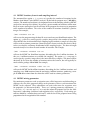
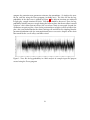
BayesAss Edition 3.0 User’s Manual
Bruce Rannala
c
2007
University of California Davis
Last updated 7 October 2011
1
Installation
The latest version of BA3 can be downloaded here. Unzip the archive by double clicking
the downloaded file. A folder will be created in your current directory containing the
program source code, documentation, and precompiled binary files for various computer
operating systems. If you have a compiler and are adventurous you can try compiling the
source code (see below), otherwise refer to the instructions below to use a precompiled
binary file for your specific computer operating system.
1.1
Mac OS X
Download the zip archived file with the latest version of the software here. Unzip the
archive by double clicking the downloaded file. A folder will be created in your current directory containing the program executable file BA3, example data files (in subfolder
examples), and the manual (in subfolder docs).
1.2
Windows
A Windows binary for BA3 is not yet available.
1.3
Compiling the program
The source code for the program is found in the source tarball distribution file named
BA3-*.*.*.tar.gz where * indicate the version numbers. The program uses routines
from the gnu scientific library (gsl) and this library (and header files) must be installed
prior to compiling. The gsl library can be found here. If using a command line C++
compiler (e.g., g++, c++, etc), with gsl installed, simply execute the following terminal
commands in the directory that contains the source tarball:
1
tar -xvzf BA3-*.tar.gz
cd BA3-*
./configure
./make all
sudo ./make install
This should install the executable file BA3 into an appropriate bin directory that is in the
user’s default shell path (often /usr/bin or /local/bin) and typing BA3 at the command
prompt will then execute the program. The procedures for compiling in Windows using
the Cygwin package are essentially identical.
2
Running the program
The BA3 program is a command line program. If you are familiar with the unix terminal you will find it straightforward to use as it adheres to standard unix conventions for
command line options, etc. If you have never used a terminal (command line) program
you can find a beginners guide here. Detailed instructions for running the program on
the Mac OS X (or other unix-based) operating system are provided below.
2.1
Getting BA3 up and running on Mac OS X or Unix
To run the program, you will first need to start the terminal application which can be
found in the Applications/Utilities folder on a Mac. A short tutorial on using the Mac OS
X terminal can be found here. The following description assumes that you have unzipped
the BA3 distribution file on the Desktop. If you have placed it elsewhere you will need to
change the commands to indicate the correct file path. Once you open terminal you will
see a command line prompt. On a Mac, at the prompt type:
cd /Users/<login>/Desktop/BA3.*/binary/macosx
where <login> is replaced with your account login name. On another unix computer you
will specify the path to the binary that you unpacked (or compiled from source code).
The unix command cd is short for “change directory” and the above command changes
the current working directory from the user’s home directory (the default) to the directory where the BA3 program binary resides. To run the program using an example data
file with 3 populations (contained in the subdirectory examples) type the following command:
./BA3 -v examples/3pop.txt
2
The prefix ./ means “current directory” and tells the operating system to look for the
program file named BA3 in the current working directory. The program option -v specifies
“verbose” output and causes BA3 to print out more detailed information to the screen
when the program is running. You should see output similar to the following:
BayesAss Version 3.0 (BA3)
Bruce Rannala
Department of Evolution and Ecology at UC Davis
Input file: examples/3pop.txt
Output file: BA3out.txt
Individuals: 400 Populations: 3 Loci: 7 Missing genotypes: 6
Locus:(Number of Alleles)
loc0:2 loc1:3 loc2:3 loc3:3 loc4:2 loc5:2 loc6:2
logP(M): -1616.27 logL(G): -3101.46 logL: -4717.74
% accepted: (0.12, 0.23, 0.67, 0.76, 0.60)
logP(M): -1617.79 logL(G): -3117.84 logL: -4735.63
% accepted: (0.12, 0.22, 0.67, 0.77, 0.60)
logP(M): -1619.86 logL(G): -3085.46 logL: -4705.33
% accepted: (0.12, 0.22, 0.67, 0.77, 0.60)
logP(M): -1619.93 logL(G): -3051.05 logL: -4670.98
% accepted: (0.12, 0.22, 0.67, 0.77, 0.60)
logP(M): -1616.75 logL(G): -3123.94 logL: -4740.70
% accepted: (0.12, 0.22, 0.67, 0.78, 0.60)
logP(M): -1619.99 logL(G): -3079.03 logL: -4699.03
% accepted: (0.12, 0.22, 0.67, 0.78, 0.60)
logP(M): -1616.92 logL(G): -3090.25 logL: -4707.17
% accepted: (0.12, 0.22, 0.67, 0.78, 0.60)
logP(M): -1616.27 logL(G): -3085.12 logL: -4701.39
% accepted: (0.12, 0.21, 0.67, 0.78, 0.60)
logP(M): -1618.92 logL(G): -3122.70 logL: -4741.62
% accepted: (0.12, 0.21, 0.67, 0.78, 0.60)
logP(M): -1621.28 logL(G): -3125.25 logL: -4746.53
% accepted: (0.12, 0.21, 0.67, 0.78, 0.60)
3
% done: (0.10)
% done: (0.20)
% done: (0.30)
% done: (0.40)
% done: (0.50)
% done: (0.60)
% done: (0.70)
% done: (0.80)
% done: (0.90)
% done: (1.00)
MCMC run completed. Output written to BA3out.txt
The program will create an output file in the current working directory when it has finished running. By default the output file is named BA3out.txt. You can double click on
this file to open it with the Mac text editor and see the results.
3
Data file format
The BA3 program uses an input file format that is identical to that of earlier BayesAss
releases. The input file should be in a plain text format. DO NOT use a word processor
such as Word to create the input file without explicitly converting it to a text file format
before use. One possible approach is to input the data into a spreadsheet program such as
Excel and then save the file as a “space-delimited text file.” Another approach is to install
one of the many available free text editors such as emacs or vi on your computer. Each
line of the input file should have the following format
indivID popID locID allele1 allele2
where indivID is a unique identifier for the individual, popID is a unique identifier of the
individual’s source population, locID is a unique identifier for the locus, and allele1
and allele2 are the allele labels for each allele of the individual’s genotype. The order of
the alleles on the line is arbitrary. Missing alleles are represented using a 0. If there are n
individuals and L loci there will be n × L lines in the input file. See the example data files
distributed with the program.
4
Command line options
The BA3 program has about a dozen command line options that allow you to control
the way the program runs and the level of detail in the output that it produces. The
command line options are given after the program name and before the input file name.
For example,
./BA3 -v -i=10000000 -o myout.txt myin.txt
executes the program for 1 million iterations using verbose output, writing the output to
the file myout.txt and using the input file myin.txt. Some options such as the option
specifying the number of iterations, -i, take parameter values while others such as -v
do not. Parameter values should follow the option specifier and may, or may not, be
separated from the option specifier by a space or an an = sign. For example, the following
are all equivalent ways to specify 1, 000, 000 iterations:
4
./BA3 -i1000000 myin.txt
./BA3 -i 1000000 myin.txt
./BA3 -i=1000000 myin.txt
Table 1 lists all the command line options with a brief description of their parameters and
effects. Each option is described in detail in the remainder of this section. Following Unix
conventions, each command line option has two possible forms, a short (one letter) form
preceded by - and a longer, one word form preceded by --, for example the ”verbose
output” command can be specified on the command line as either -v or --verbose. The
longer forms are available solely because some persons find them easier to remember.
Option
-a --deltaA
-b --burnin
-f --deltaF
-g --genotypes
-i --iterations
-m --deltaM
-n --sampling
-o- --output
-s --seed
-t --trace
-u --settings
-v --verbose
Parameter Values
0 < ∆ A ≤ 1.0
Positive integer
0 < ∆ F ≤ 1.0
None
Positive integer
0 < ∆ M ≤ 1.0
Positive integer
String
Positive integer
None
None
None
Effect
Mixing parameter for allele frequencies
Number of iterations to discard as burnin
Mixing parameter for inbreeding coefficients
Output genotypes and migrant ancestries
Number of iterations for MCMC
Mixing parameter for migration rates
Interval between samples for MCMC
Output file name
Seed for random number generator
Create a trace file to monitor convergence
Output options and parameter settings
Use verbose screen output
Table 1: Options available for BA3 program
4.1
Random number generator seed
The option -s (--seed) is used to specify a positive integer used to ”seed” the random
number generator algorithm. A deterministic algorithm is used to generate pseudorandom numbers during the MCMC such that the sequence of random numbers is entirely determined by the starting seed. Thus, separate runs of the program started using
same seed will produce exactly the same outcome. To test whether the program is converging it is important to carry out several independent runs initiated with different seeds.
To start the program using 10456 as the random number seed use the following command:
./BA3 -s=104656
If no seed is specified the default seed is 10.
5
4.2
MCMC iterations, burn-in and sampling interval
The command line option -i (--iterations) specifies the number of iterations for the
Markov chain Monte Carlo (MCMC) analysis. By default the program uses 5, 000, 000 iterations. The number of iterations is an important factor in determining whether a MCMC
analysis has converged (see below). In general, a greater number of iterations will be more
likely to insure convergence but the run-time of the program also increases in proportion
to the number of iterations. The value of the number of iterations should be a positive
integer. For example,
.\BA3 -i10000000 test.txt
will execute the program using the data file test.txt and carry out 10 million iterations. The
option -b (--burnin) is used to specify a positive integer that is the number of iterations
of the MCMC that are discarded before sampling begins to obtain a sample of values that
will be used to estimate parameters. Burn-in length is chosen such that the chain is likely
to have reached the stationary distribution before sampling begins. The burn-in length
must obviously be less than the total number of iterations. For example,
./BA3
-i10000000 -b1000000 test.txt
will run the MCMC for 10 million iterations, discarding the first 1 million iterations. In
this case, 9 million iterations are available for sampling. The option -n (--sampling) is
used to specify a positive integer that is the interval between samples. This interval must
obviously be less than the number of iterations minus the burn-in, but will typically be
much smaller, perhaps 100 or 1000. For example,
./BA3
-i10000000 -b1000000 -n1000 test.txt
will run the MCMC for 10 million iterations, discarding the first 1 million iterations and
sampling every 1000 iterations from the remaining 9 million iterations, producing a sample of 9000 observations from the chain that will be used to estimate parameters.
4.3
MCMC mixing parameters
For continuous parameters such as migration rates, allele frequencies and inbreeding coefficients, the size of the proposed change to the parameter value at each iteration of the
MCMC can be adjusted. These adjustments are used to fine-tune the acceptance rates
for proposals (see discussion below). There are 3 mixing parameter adjustments: -a
(--deltaA), -f (--deltaF) and -m (--deltaM) that adjust the proposal size for the allele
frequencies, inbreeding coefficients and migration rates, respectively. Each mixing parameter should be a number between 0 and 1, with the size of the proposed move being
proportional to the magnitude of this number.
6
4.4
Options for printing output
By default, the output produced by BA3 is written to a file named BA3out.txt that the
program creates in the current working directory. An alternative name for the output file
can be specified using the option -o (--output). For example,
./BA3 -o myout.txt test.txt
executes the program using the input file test.txt and writes the output to a file named
myout.txt. The option -t (--trace) specifies whether a trace output file is created that
lists all the parameter values at each iteration of the MCMC run. If this option is specified
a file named BA3trace.txt is created in the current working directory. This file can be
used to monitor convergence of the MCMC by plotting the profile of the likelihood and
prior values, as well as those of various parameters, over time, using a program such as
Tracer (see below). The option -g causes detailed information regarding the individual
multilocus genotypes and posterior probabilities of migrant ancestries to be written to a
file named BA3indiv.txt created in the current working directory. The option -u specifies
that current values of command line options are printed at the beginning of the output
file (recommended). Finally, the option -v (--verbose) specifies that detailed information
about the input data (number of populations. number of loci, number of individuals, and
so on) is written to the computer screen during the run and that likelihoods and parameter
acceptance rates are written to the computer screen as the program runs (recommended).
This detailed output can be used to adjust mixing parameters during initial trial runs (see
below). It is also useful for checking that the input file is in the correct format and the data
are being read correctly by the program.
5
Recommendations for running BA3
To generate correct results using BA3 it is important to adjust the mixing parameters,
use a sufficient number of iterations, discard enough iterations as burn-in, and carry out
several independent runs (started with different random number seeds), examining the
trace files for evidence of convergence and mixing and looking for consistency of the
estimates between independent runs. Here I will outline a general strategy for achieving
this. I illustrate the strategy using the example data file 3pop.txt. I will begin with an
explanation of the screen output generated using option -v.
5.1
Understanding BA3 screen output
Running the BA3 program using the command ./BA3 -v examples/3pop.txt produces
the following screen output:
BayesAss Version 3.0 (BA3)
7
Bruce Rannala
Department of Evolution and Ecology at UC Davis
Input file: examples/3pop.txt
Output file: BA3out.txt
Individuals: 400 Populations: 3 Loci: 7 Missing genotypes: 6
Locus:(Number of Alleles)
loc0:2 loc1:3 loc2:3 loc3:3 loc4:2 loc5:2 loc6:2
The first two lines of screen output (following the program title) specify the names of the
input and output files. The next line prints the number of individuals (in this case, 400),
the number of populations (in this case, 3), the number of loci (in this case, 7), and the
total number of missing genotypes (in this case, 6). This is followed by a line specifying
the number of alleles present at each locus. You should check that all these values agree
with the expectations for your data. Discrepancies can indicate that there is a formatting
error and the input file is not being read correctly. Once the MCMC begins running the
current state of the chain will be printed to screen as follows:
logP(M): -1618.76 logL(G): -3087.23 logL: -4705.99 % done: [0.07]
% accepted: (0.31, 0.25, 0.66, 0.76, 0.60)
The first value logP(M) is the log probability of the current configuration of migrant ancestries among individuals, conditional on the current migration rates. The second value
logL(G) is the log-likelihood of the genotype data given the migrant ancestries of individuals and the current population allele frequencies. The third value logL is the sum of
these two terms. The value in brackets (or parentheses) after done is the percentage of the
total iterations that have been completed. This proportion is displayed in square brackets
if the chain is still in the burn-in phase, otherwise it is displayed in parentheses. The final
output after % accepted is the acceptance rate for proposed changes to each of the 5 parameters from left to right: (1) migration rates; (2) individual migrant ancestries; (3) allele
frequencies; (4) inbreeding coefficients; (5) missing genotypes.
5.2
Adjustment of mixing parameters
The acceptance rates for proposed changes to parameters 1, 3 and 4 in the above list (migration rates, allele frequencies and inbreeding coefficients, respectively) can be adjusted
by changing the values of the respective mixing parameters. If the acceptance rate is too
high, the chain does not mix well, often proposing values very near the current value
8
(which are accepted) and failing to adequately explore the state space. If the acceptance
rate is too low the chain rarely accepts the proposed moves which are too different from
the current value – this also causes poor mixing. Empirical analyses suggest that an acceptance rate between 20% and 40% is optimal. In the above example, the acceptance rate
for proposed changes to migration rate is about 31 % which is adequate. However, the acceptance rates for proposed changes to the allele frequencies and inbreeding coefficients
are 66% and 76% respectively, which are both too high. One can decrease the acceptance
rate by proposing larger moves (or increase the rate by proposing smaller ones). In this
case, we want to decrease the acceptance rate so we will try increasing the proposal step
size for the mixing parameters associated with proposed moves of both the allele frequencies and inbreeding coefficients. The default values of all the mixing parameters are 0.10.
We will try increasing the proposal step length to 0.30 for both these proposals. Stop
the program by typing Control-C in the terminal, then start it again using the following
command options:
./BA3 -v -a0.30 -f0.30 examples/3pop.txt
The output from the MCMC run is now as follows:
logP(M): -1618.75 logL(G): -3142.41 logL: -4761.16 % done: [0.07]
% accepted: (0.31, 0.24, 0.31, 0.45, 0.60)
This is much better, but the acceptance rate for proposed changes to the inbreeding coefficients is still a bit high at 45%. We therefore again kill the program run using Control-C
and try again with the following mixing parameters:
./BA3 -v -a0.30 -f0.50 examples/3pop.txt
The output from the MCMC run is now as follows:
logP(M): -1618.38 logL(G): -3115.25 logL: -4733.63 % done: [0.08]
% accepted: (0.31, 0.24, 0.32, 0.33, 0.60)
The acceptance rates now look okay so we will next try some longer runs with these values
for the mixing parameters and create a trace file to examine convergence.
5.3
Diagnosing convergence
Enter the following to initiate a longer run with the random seed 100, creating a trace file
and printing the output to a file named run1out.txt:
./BA3 -v -a0.30 -f0.50 -t -s100 -i10000000 -b1000000 -n100 \
-o run1out.txt examples/3pop.txt
The contents of the output file run1out.txt are as follows:
9
Input file: examples/3pop.txt
Individuals: 400 Populations: 3 Loci: 7
Locus:(Number of Alleles)
loc0:2 loc1:3 loc2:3 loc3:3 loc4:2 loc5:2 loc6:2
Population Index -> Population Label:
0->pop0 1->pop1 2->pop2
Migration Rates:
m[0][0]: 0.9718(0.0115) m[0][1]: 0.0130(0.0100) m[0][2]: 0.0152(0.0090)
m[1][0]: 0.0878(0.0141) m[1][1]: 0.7338(0.0396) m[1][2]: 0.1784(0.0407)
m[2][0]: 0.0870(0.0179) m[2][1]: 0.2047(0.0326) m[2][2]: 0.7083(0.0292)
Inbreeding Coefficients:
pop0 Fstat: 0.2552(0.0367)
pop1 Fstat: 0.0810(0.0588)
pop2 Fstat: 0.2698(0.0891)
Allele Frequencies:
pop0
loc0>>
2:0.806(0.029)
loc1>>
3:0.309(0.033)
loc2>>
2:0.751(0.031)
loc3>>
2:0.384(0.035)
loc4>>
1:0.825(0.028)
loc5>>
2:0.234(0.031)
loc6>>
2:0.237(0.031)
1:0.194(0.029)
2:0.601(0.035) 1:0.089(0.020)
3:0.170(0.027) 1:0.078(0.018)
1:0.292(0.032) 3:0.324(0.032)
2:0.175(0.028)
1:0.766(0.031)
1:0.763(0.031)
10
pop1
loc0>>
2:0.512(0.065)
loc1>>
3:0.323(0.068)
loc2>>
2:0.222(0.062)
loc3>>
2:0.663(0.069)
loc4>>
1:0.266(0.071)
loc5>>
2:0.750(0.049)
loc6>>
2:0.868(0.058)
pop2
loc0>>
2:0.479(0.077)
loc1>>
3:0.451(0.083)
loc2>>
2:0.195(0.070)
loc3>>
2:0.465(0.069)
loc4>>
1:0.121(0.068)
loc5>>
2:0.862(0.053)
loc6>>
2:0.779(0.062)
1:0.488(0.065)
2:0.445(0.070) 1:0.232(0.075)
3:0.593(0.061) 1:0.186(0.054)
1:0.325(0.071) 3:0.012(0.012)
2:0.734(0.071)
1:0.250(0.049)
1:0.132(0.058)
1:0.521(0.077)
2:0.176(0.068) 1:0.374(0.080)
3:0.433(0.077) 1:0.372(0.072)
1:0.506(0.069) 3:0.029(0.017)
2:0.879(0.068)
1:0.138(0.053)
1:0.221(0.062)
The first few lines of output summarize properties of the data. Next, there is a line that
maps an integer index to each population label. This is done simply to allow the between
population migration matrix to be printed more concisely. Next is the matrix of inferred
(posterior mean) migration rates and the standard deviation of the marginal posterior
distribution for each estimate. A rough 95% credible set can be constructed as mean ±
1.96 × sdev. Next are the mean posterior estimates (and standard errors) of inbreeding
coefficients and allele frequencies for each locus and population. Two simple ways to
examine convergence are: (1) conduct multiple runs initialized with different seeds and
11
compare the posterior mean parameter estimates for concordance. (2) Analyze the trace
file for each run using the Tracer program (available here). The trace file for the logprobability of the above run is plotted in Figure 1. The burn-in iterations are indicated
in light grey, sample iterations in black. Two things should be observed. First, the logprobability initially increases steeply during the burn-in phase but then oscillates around
a plateau – this is often (but not always) the case when a chain as converged. Second, the
oscillations are quite regular – there are no persistant lows or highs (valleys or hills) in the
plot – this is one indication that the chain is mixing well and effectively sampling from the
posterior distribution with less autocorrelation between successive samples of the chain
than would be the case if valleys and hills existed.
Figure 1: Trace file for log probability in a BA3 analysis of example input file 3pop.txt
created using the Tracer program
12