Download PyMC: Bayesian Stochastic Modelling in Python

Journal of Statistical Software
JSS
July 2010, Volume 35, Issue 4.
http://www.jstatsoft.org/
PyMC: Bayesian Stochastic Modelling in Python
Anand Patil
David Huard
Christopher J. Fonnesbeck
University of Oxford
McGill University
Vanderbilt University
Abstract
This user guide describes a Python package, PyMC, that allows users to efficiently
code a probabilistic model and draw samples from its posterior distribution using Markov
chain Monte Carlo techniques.
Keywords: Bayesian modeling, Markov chain Monte Carlo, simulation, Python.
1. Introduction
1.1. Purpose
PyMC is a python module that implements Bayesian statistical models and fitting algorithms,
including Markov chain Monte Carlo. Its flexibility and extensibility make it applicable to a
large suite of problems. Along with core sampling functionality, PyMC includes methods for
summarizing output, plotting, goodness-of-fit and convergence diagnostics.
1.2. Features
PyMC provides functionalities to make Bayesian analysis as painless as possible. It fits
Bayesian statistical models with Markov chain Monte Carlo and other algorithms. Traces
can be saved to the disk as plain text, Python pickles, SQLite (The SQLite Development
Team 2010) or MySQL (Oracle Corporation 2010) database, or HDF5 (The HDF Group
2010) archives. Summaries including tables and plots can be created from these, and several
convergence diagnostics are available. Sampling loops can be paused and tuned manually, or
saved and restarted later. MCMC loops can be embedded in larger programs, and results can
be analyzed with the full power of Python.
PyMC includes a large suite of well-documented statistical distributions which use NumPy
(Oliphant 2006) and hand-optimized Fortran routines wherever possible for performance. It
2
PyMC: Bayesian Stochastic Modelling in Python
also includes a module for modeling Gaussian processes. Equally importantly, PyMC can
easily be extended with custom step methods and unusual probability distributions.
1.3. Usage
First, define your model in a file, say mymodel.py:
import pymc
import numpy as np
n = 5*np.ones(4,dtype=int)
x = np.array([-.86,-.3,-.05,.73])
alpha = pymc.Normal('alpha',mu=0,tau=.01)
beta = pymc.Normal('beta',mu=0,tau=.01)
@pymc.deterministic
def theta(a=alpha, b=beta):
"""theta = logit^{-1}(a+b)"""
return pymc.invlogit(a+b*x)
d = pymc.Binomial('d', n=n, p=theta, value=np.array([0.,1.,3.,5.]),\
observed=True)
Save this file, then from a Python shell (or another file in the same directory), call:
import pymc
import mymodel
S = pymc.MCMC(mymodel, db = 'pickle')
S.sample(iter = 10000, burn = 5000, thin = 2)
pymc.Matplot.plot(S)
This example will generate 10000 posterior samples, thinned by a factor of 2, with the first
half discarded as burn-in. The sample is stored in a Python serialization (pickle) database.
1.4. History
PyMC began development in 2003, as an effort to generalize the process of building MetropolisHastings samplers, with an aim to making Markov chain Monte Carlo (MCMC) more accessible to non-statisticians (particularly ecologists). The choice to develop PyMC as a Python
module, rather than a standalone application, allowed the use MCMC methods in a larger
modeling framework. By 2005, PyMC was reliable enough for version 1.0 to be released to
the public. A small group of regular users, most associated with the University of Georgia,
provided much of the feedback necessary for the refinement of PyMC to a usable state.
In 2006, David Huard and Anand Patil joined Chris Fonnesbeck on the development team for
PyMC 2.0. This iteration of the software strives for more flexibility, better performance and
a better end-user experience than any previous version of PyMC.
Journal of Statistical Software
3
PyMC 2.1 has been released in early 2010. It contains numerous bugfixes and optimizations,
as well as a few new features. This user guide is written for version 2.1.
1.5. Relationship to other packages
PyMC in one of many general-purpose MCMC packages. The most prominent among them is
WinBUGS (Spiegelhalter, Thomas, Best, and Lunn 2003; Lunn, Thomas, Best, and Spiegelhalter 2000), which has made MCMC and with it Bayesian statistics accessible to a huge
user community. Unlike PyMC, WinBUGS is a stand-alone, self-contained application. This
can be an attractive feature for users without much programming experience, but others may
find it constraining. A related package is JAGS (Plummer 2003), which provides a more
Unix-like implementation of the BUGS language. Other packages include Hierarchical Bayes
Compiler (Daumé III 2007) and a number of R (R Development Core Team 2010) packages,
for example MCMCglmm (Hadfield 2010) and MCMCpack (Martin, Quinn, and Park 2009).
It would be difficult to meaningfully benchmark PyMC against these other packages because
of the unlimited variety in Bayesian probability models and flavors of the MCMC algorithm.
However, it is possible to anticipate how it will perform in broad terms.
PyMC’s number-crunching is done using a combination of industry-standard libraries (NumPy,
Oliphant 2006, and the linear algebra libraries on which it depends) and hand-optimized Fortran routines. For models that are composed of variables valued as large arrays, PyMC will
spend most of its time in these fast routines. In that case, it will be roughly as fast as packages written entirely in C and faster than WinBUGS. For finer-grained models containing
mostly scalar variables, it will spend most of its time in coordinating Python code. In that
case, despite our best efforts at optimization, PyMC will be significantly slower than packages
written in C and on par with or slower than WinBUGS. However, as fine-grained models are
often small and simple, the total time required for sampling is often quite reasonable despite
this poorer performance.
We have chosen to spend time developing PyMC rather than using an existing package primarily because it allows us to build and efficiently fit any model we like within a full-fledged
Python environment. We have emphasized extensibility throughout PyMC’s design, so if it
doesn’t meet your needs out of the box chances are you can make it do so with a relatively
small amount of code. See the testimonials page (http://code.google.com/p/pymc/wiki/
Testimonials) for reasons why other users have chosen PyMC.
1.6. Getting started
This guide provides all the information needed to install PyMC, code a Bayesian statistical
model, run the sampler, save and visualize the results. In addition, it contains a list of the
statistical distributions currently available. More examples of usage as well as tutorials are
available from the PyMC web site at http://code.google.com/p/pymc.
2. Installation
2.1. Dependencies
PyMC requires some prerequisite packages to be present on the system. Fortunately, there
4
PyMC: Bayesian Stochastic Modelling in Python
are currently only a few dependencies, and all are freely available online.
ˆ Python version 2.5 or 2.6.
ˆ NumPy (1.4 or newer): The fundamental scientific programming package, it provides a
multidimensional array type and many useful functions for numerical analysis.
ˆ matplotlib (Hunter 2007), optional: 2D plotting library which produces publication
quality figures in a variety of image formats and interactive environments
ˆ PyTables (Alted, Vilata, Prater, Mas, Hedley, Valentino, and Whitaker 2010), optional:
Package for managing hierarchical datasets and designed to efficiently and easily cope
with extremely large amounts of data. Requires the HDF5 library.
ˆ pydot (Carrera and Theune 2010), optional: Python interface to Graphviz (Gansner
and North 1999), it allows PyMC to create both directed and non-directed graphical
representations of models.
ˆ SciPy (Jones, Oliphant, and Peterson 2001), optional: Library of algorithms for mathematics, science and engineering.
ˆ IPython (Pérez and Granger 2007) , optional: An enhanced interactive Python shell and
an architecture for interactive parallel computing.
ˆ nose (Pellerin 2010), optional: A test discovery-based unittest extension (required to
run the test suite).
There are prebuilt distributions that include all required dependencies. For Mac OS X users,
we recommend the MacPython (Python Software Foundation 2005) distribution or the Enthought Python distribution (Enthought, Inc. 2010) on OS X 10.5 (Leopard) and Python 2.6.1
that ships with OS X 10.6 (Snow Leopard). Windows users should download and install
the Enthought Python Distribution. The Enthought Python distribution comes bundled with
these prerequisites. Note that depending on the currency of these distributions, some packages
may need to be updated manually.
If instead of installing the prebuilt binaries you prefer (or have) to build PyMC yourself,
make sure you have a Fortran and a C compiler. There are free compilers (gfortran, gcc, Free
Software Foundation, Inc. 2010) available on all platforms. Other compilers have not been
tested with PyMC but may work nonetheless.
2.2. Installation using EasyInstall
The easiest way to install PyMC is to type in a terminal:
easy_install pymc
Provided EasyInstall (part of the setuptools module, Eby 2010) is installed and in your
path, this should fetch and install the package from the Python Package Index at http:
//pypi.python.org/pypi. Make sure you have the appropriate administrative privileges to
install software on your computer.
Journal of Statistical Software
5
2.3. Installing from pre-built binaries
Pre-built binaries are available for Windows XP and Mac OS X. There are at least two ways
to install these. First, you can download the installer for your platform from the Python
Package Index. Alternatively, you can double-click the executable installation package, then
follow the on-screen instructions.
For other platforms, you will need to build the package yourself from source. Fortunately,
this should be relatively straightforward.
2.4. Compiling the source code
First, download the source code tarball from the Python Package Index and unpack it. Then
move into the unpacked directory and follow the platform specific instructions.
Windows
One way to compile PyMC on Windows is to install MinGW (Peters 2010) and MSYS.
MinGW is the GNU Compiler Collection (gcc) augmented with Windows specific headers and
libraries. MSYS is a POSIX-like console (bash) with Unix command line tools. Download
the Automated MinGW Installer from http://sourceforge.net/projects/mingw/files/
and double-click on it to launch the installation process. You will be asked to select which
components are to be installed: make sure the g77 (Free Software Foundation, Inc. 2010)
compiler is selected and proceed with the instructions. Then download and install http:
//downloads.sourceforge.net/mingw/MSYS-1.0.11.exe, launch it and again follow the
on-screen instructions.
Once this is done, launch the MSYS console, change into the PyMC directory and type:
python setup.py install
This will build the C and Fortran extension and copy the libraries and Python modules in the
C:/Python26/Lib/site-packages/pymc directory.
Mac OS X or Linux
In a terminal, type:
python setup.py config_fc --fcompiler=gnu95 build
python setup.py install
The above syntax also assumes that you have gfortran installed and available. The sudo
command may be required to install PyMC into the Python site-packages directory if it
has restricted privileges.
2.5. Development version
You can clone out the bleeding edge version of the code from the git (Torvalds 2010) repository:
git clone git://github.com/pymc-devs/pymc
6
PyMC: Bayesian Stochastic Modelling in Python
2.6. Running the test suite
PyMC comes with a set of tests that verify that the critical components of the code work as
expected. To run these tests, users must have nose installed. The tests are launched from a
Python shell:
import pymc
pymc.test()
In case of failures, messages detailing the nature of these failures will appear.
2.7. Bugs and feature requests
Report problems with the installation, test failures, bugs in the code or feature request on
the issue tracker at http://code.google.com/p/pymc/issues/list, specifying the version
you are using and the environment. Comments and questions are welcome and should be
addressed to PyMC’s mailing list at [email protected].
3. Tutorial
This tutorial will guide you through a typical PyMC application. Familiarity with Python is
assumed, so if you are new to Python, books such as Lutz (2007) or Langtangen (2009) are the
place to start. Plenty of online documentation can also be found on the Python documentation
page at http://www.python.org/doc/.
3.1. An example statistical model
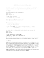
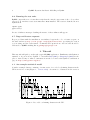
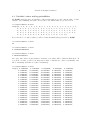
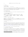
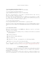
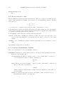
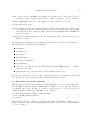
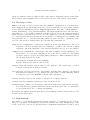
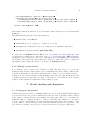
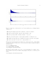
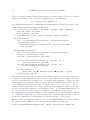
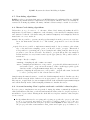
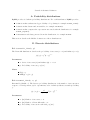
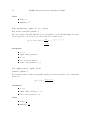
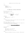
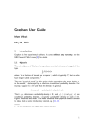
Consider a sample dataset consisting of a time series of recorded coal mining disasters in the
UK from 1851 to 1962 (Figure 1, Jarrett 1979). Occurrences of disasters in the series is
6
number of disasters
5
4
3
2
1
0
1860
1880
1900
year
1920
1940
Figure 1: Recorded coal mining disasters in the UK.
1960
Journal of Statistical Software
7
thought to be derived from a Poisson process with a large rate parameter in the early part
of the time series, and from one with a smaller rate in the later part. We are interested in
locating the change point in the series, which perhaps is related to changes in mining safety
regulations.
We represent our conceptual model formally as a statistical model:
e if t < s
(Dt |s, e, l) ∼ Poisson (rt ) , rt =
, t ∈ [tl , th ]
l if t ≥ s
s ∼ Discrete Uniform(tl , th )
e ∼ Exponential(re )
l ∼ Exponential(rl )
(1)
The symbols are defined as:
Dt : The number of disasters in year t.
rt : The rate parameter of the Poisson distribution of disasters in year t.
s: The year in which the rate parameter changes (the switchpoint).
e: The rate parameter before the switchpoint s.
l: The rate parameter after the switchpoint s.
tl , th : The lower and upper boundaries of year t.
re , rl : The rate parameters of the priors of the early and late rates, respectively.
Because we have defined D by its dependence on s, e and l, the latter three are known as the
‘parents’ of D and D is called their ‘child’. Similarly, the parents of s are tl and th , and s is
the child of tl and th .
3.2. Two types of variables
At the model-specification stage (before the data are observed), D, s, e, r and l are all random
variables. Bayesian ‘random’ variables have not necessarily arisen from a physical random
process. The Bayesian interpretation of probability is epistemic, meaning random variable
x’s probability distribution p(x) represents our knowledge and uncertainty about x’s value
(Jaynes 2003). Candidate values of x for which p(x) is high are relatively more probable,
given what we know. Random variables are represented in PyMC by the classes Stochastic
and Deterministic.
The only Deterministic in the model is r. If we knew the values of r’s parents (s, l and e), we
could compute the value of r exactly. A Deterministic like r is defined by a mathematical
function that returns its value given values for its parents. Deterministic variables are
sometimes called the systemic part of the model. The nomenclature is a bit confusing, because
these objects usually represent random variables; since the parents of r are random, r is
random also. A more descriptive (though more awkward) name for this class would be
DeterminedByValuesOfParents.
On the other hand, even if the values of the parents of variables s, D (before observing the
data), e or l were known, we would still be uncertain of their values. These variables are
8
PyMC: Bayesian Stochastic Modelling in Python
characterized by probability distributions that express how plausible their candidate values
are, given values for their parents. The Stochastic class represents these variables. A more
descriptive name for these objects might be RandomEvenGivenValuesOfParents.
We can represent model 1 in a file called DisasterModel.py (the actual file can be found in
pymc/examples/) as follows. First, we import the PyMC and NumPy namespaces:
from pymc import DiscreteUniform, Exponential, deterministic, Poisson, Uniform
import numpy
Notice that from pymc we have only imported a select few objects that are needed for this
particular model, whereas the entire numpy namespace has been imported.
Next, we enter the actual data values into an array:
disasters_array =
\
numpy.array([ 4,
3,
2,
1,
0,
3,
0,
5,
3,
2,
0,
1,
3,
0,
4,
5,
3,
1,
0,
1,
0,
0,
4,
4,
1,
1,
1,
1,
1,
5,
2,
0,
0,
2,
0,
4,
3,
1,
0,
0,
1,
0,
3,
1,
3,
3,
0,
1,
0,
4,
4,
2,
1,
2,
1,
0,
0,
4,
2,
0,
1,
1,
0,
6,
1,
1,
3,
0,
2,
1,
3,
5,
1,
2,
0,
4,
0,
3,
5,
1,
2,
0,
2,
0,
4,
3,
1,
0,
1,
0,
1,
0,
4,
3,
1,
1,
0,
0,
2, 6,
2, 5,
0, 0,
1, 1,
0, 2,
1, 4,
1])
Note that you don’t have to type in this entire array to follow along; the code is available
in the source tree, in pymc/examples/DisasterModel.py. Next, we create the switchpoint
variable s:
s = DiscreteUniform('s', lower=0, upper=110, doc='Switchpoint[year]')
DiscreteUniform is a subclass of Stochastic that represents uniformly-distributed discrete
variables. Use of this distribution suggests that we have no preference a priori regarding the
location of the switchpoint; all values are equally likely. Now we create the exponentiallydistributed variables e and l for the early and late Poisson rates, respectively:
e = Exponential('e', beta=1)
l = Exponential('l', beta=1)
Next, we define the variable r, which selects the early rate e for times before s and the late
rate l for times after s. We create r using the deterministic decorator, which converts the
ordinary Python function r into a Deterministic object.
@deterministic(plot=False)
def r(s=s, e=e, l=l):
""" Concatenate Poisson means """
out = numpy.empty(len(disasters_array))
out[:s] = e
out[s:] = l
return out
Journal of Statistical Software
9
The last step is to define the number of disasters D. This is a stochastic variable, but unlike
s, e and l we have observed its value. To express this, we set the argument observed to
True (it is set to False by default). This tells PyMC that this object’s value should not be
changed:
D = Poisson('D', mu=r, value=disasters_array, observed=True)
3.3. Why are data and unknown variables represented by the same object?
Since it is represented by a Stochastic object, D is defined by its dependence on its parent r
even though its value is fixed. This isn’t just a quirk of PyMC’s syntax; Bayesian hierarchical
notation itself makes no distinction between random variables and data. The reason is simple:
to use Bayes’ theorem to compute the posterior p(e, s, l|D) of model (1), we require the
likelihood p(D|e, s, l). Even though D’s value is known and fixed, we need to formally assign
it a probability distribution as if it were a random variable. Remember, the likelihood and the
probability function are essentially the same, except that the former is regarded as a function
of the parameters and the latter as a function of the data.
This point can be counterintuitive at first, as many peoples’ instinct is to regard data as fixed
a priori and unknown variables as dependent on the data. One way to understand this is to
think of statistical models like (1) as predictive models for data, or as models of the processes
that gave rise to data. Before observing the value of D, we could have sampled from its prior
predictive distribution p(D) (i.e., the marginal distribution of the data) as follows:
1. Sample e, s and l from their priors.
2. Sample D conditional on these values.
Even after we observe the value of D, we need to use this process model to make inferences
about e, s and l because its the only information we have about how the variables are related.
3.4. Parents and children
We have above created a PyMC probability model, which is simply a linked collection of
variables. To see the nature of the links, import or run DisasterModel.py and examine s’s
parents attribute from the Python prompt:
>>> from pymc.examples import DisasterModel
>>> DisasterModel.s.parents
{`lower': 0, 'upper': 110}
The parents dictionary shows us the distributional parameters of s, which are constants.
Now let’s examinine D’s parents:
>>> DisasterModel.D.parents
{`mu': <pymc.PyMCObjects.Deterministic 'r' at 0x3e51a70>}
We are using r as a distributional parameter of D (i.e., r is D’s parent). D internally labels
r as mu, meaning r plays the role of the rate parameter in D’s Poisson distribution. Now
examine r’s children attribute:
10
PyMC: Bayesian Stochastic Modelling in Python
e
l
e
s
l
s
r
mu
D
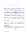
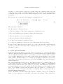
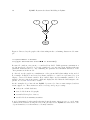
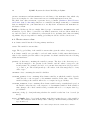
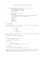
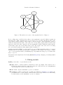
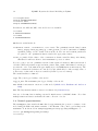
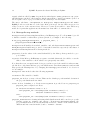
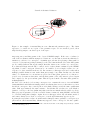
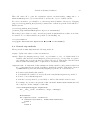
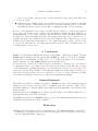
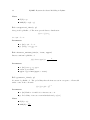
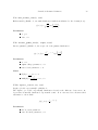
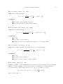
Figure 2: Directed acyclic graph of the relationships in the coal mining disaster model example.
>>> DisasterModel.r.children
set([<pymc.distributions.Poisson 'D' at 0x3e51290>])
Because D considers r its parent, r considers D its child. Unlike parents, children is a
set (an unordered collection of objects); variables do not associate their children with any
particular distributional role. Try examining the parents and children attributes of the
other parameters in the model.
A ‘directed acyclic graph’ is a visualization of the parent-child relationships in the model.
For example, in Figure 2 unobserved stochastic variables s, e and l are represented by open
ellipses, observed stochastic variable D is a filled ellipse and deterministic variable r is a
triangle. Arrows point from parent to child and display the label that the child assigns to the
parent. See Section 4.12 for more details.
As the examples above have shown, PyMC objects need to have a name assigned, such as
lower, upper or e. These names are used for storage and post-processing:
ˆ as keys in on-disk databases,
ˆ as node labels in model graphs,
ˆ as axis labels in plots of traces,
ˆ as table labels in summary statistics.
A model instantiated with variables having identical names raises an error to avoid name
conflicts in the database storing the traces. In general however, PyMC uses references to the
objects themselves, not their names, to identify variables.
Journal of Statistical Software
11
3.5. Variables’ values and log-probabilities
All PyMC variables have an attribute called value that stores the current value of that
variable. Try examining D’s value, and you’ll see the initial value we provided for it:
>>> DisasterModel.D.value
array([4, 5, 4, 0, 1, 4, 3, 4, 0, 6, 3, 3, 4, 0, 2, 6, 3, 3, 5, 4, 5, 3, 1,
4, 4, 1, 5, 5, 3, 4, 2, 5, 2, 2, 3, 4, 2, 1, 3, 2, 2, 1, 1, 1, 1, 3,
0, 0, 1, 0, 1, 1, 0, 0, 3, 1, 0, 3, 2, 2, 0, 1, 1, 1, 0, 1, 0, 1, 0,
0, 0, 2, 1, 0, 0, 0, 1, 1, 0, 2, 3, 3, 1, 1, 2, 1, 1, 1, 1, 2, 4, 2,
0, 0, 1, 4, 0, 0, 0, 1, 0, 0, 0, 0, 0, 1, 0, 0, 1, 0, 1])
If you check e’s, s’s and l’s values, you’ll see random initial values generated by PyMC:
>>> DisasterModel.s.value
44
>>> DisasterModel.e.value
0.33464706250079584
>>> DisasterModel.l.value
2.6491936762267811
Of course, since these are Stochastic elements, your values will be different than these. If
you check r’s value, you’ll see an array whose first s elements are e (here 0.33464706), and
whose remaining elements are l (here 2.64919368):
>>> DisasterModel.r.value
array([ 0.33464706, 0.33464706,
0.33464706, 0.33464706,
0.33464706, 0.33464706,
0.33464706, 0.33464706,
0.33464706, 0.33464706,
0.33464706, 0.33464706,
0.33464706, 0.33464706,
0.33464706, 0.33464706,
0.33464706, 0.33464706,
2.64919368, 2.64919368,
2.64919368, 2.64919368,
2.64919368, 2.64919368,
2.64919368, 2.64919368,
2.64919368, 2.64919368,
2.64919368, 2.64919368,
2.64919368, 2.64919368,
2.64919368, 2.64919368,
2.64919368, 2.64919368,
2.64919368, 2.64919368,
2.64919368, 2.64919368,
0.33464706,
0.33464706,
0.33464706,
0.33464706,
0.33464706,
0.33464706,
0.33464706,
0.33464706,
0.33464706,
2.64919368,
2.64919368,
2.64919368,
2.64919368,
2.64919368,
2.64919368,
2.64919368,
2.64919368,
2.64919368,
2.64919368,
2.64919368,
0.33464706,
0.33464706,
0.33464706,
0.33464706,
0.33464706,
0.33464706,
0.33464706,
0.33464706,
0.33464706,
2.64919368,
2.64919368,
2.64919368,
2.64919368,
2.64919368,
2.64919368,
2.64919368,
2.64919368,
2.64919368,
2.64919368,
2.64919368,
0.33464706,
0.33464706,
0.33464706,
0.33464706,
0.33464706,
0.33464706,
0.33464706,
0.33464706,
2.64919368,
2.64919368,
2.64919368,
2.64919368,
2.64919368,
2.64919368,
2.64919368,
2.64919368,
2.64919368,
2.64919368,
2.64919368,
2.64919368,
12
PyMC: Bayesian Stochastic Modelling in Python
2.64919368,
2.64919368,
2.64919368,
2.64919368,
2.64919368,
2.64919368,
2.64919368,
2.64919368,
2.64919368,
2.64919368])
To compute its value, r calls the funtion we used to create it, passing in the values of its
parents.
Stochastic objects can evaluate their probability mass or density functions at their current
values given the values of their parents. The logarithm of a stochastic object’s probability
mass or density can be accessed via the logp attribute. For vector-valued variables like D,
the logp attribute returns the sum of the logarithms of the joint probability or density of all
elements of the value. Try examining s’s and D’s log-probabilities and e’s and l’s log-densities:
>>> DisasterModel.s.logp
-4.7095302013123339
>>> DisasterModel.D.logp
-1080.5149888046033
>>> DisasterModel.e.logp
-0.33464706250079584
>>> DisasterModel.l.logp
-2.6491936762267811
Stochastic objects need to call an internal function to compute their logp attributes, as r
needed to call an internal function to compute its value. Just as we created r by decorating
a function that computes its value, it’s possible to create custom Stochastic objects by
decorating functions that compute their log-probabilities or densities (see Section 4). Users
are thus not limited to the set of of statistical distributions provided by PyMC.
3.6. Using variables as parents of other variables
Let’s take a closer look at our definition of r:
@deterministic(plot=False)
def r(s=s, e=e, l=l):
""" Concatenate Poisson means """
out = numpy.empty(len(disasters_array))
out[:s] = e
out[s:] = l
return out
The arguments s, e and l are Stochastic objects, not numbers. Why aren’t errors raised
when we attempt to slice array out up to a Stochastic object?
Whenever a variable is used as a parent for a child variable, PyMC replaces it with its value
attribute when the child’s value or log-probability is computed. When r’s value is recomputed,
s.value is passed to the function as argument s. To see the values of the parents of r all
together, look at r.parents.value.
Journal of Statistical Software
13
3.7. Fitting the model with MCMC
PyMC provides several objects that fit probability models (linked collections of variables) like
ours. The primary such object, MCMC, fits models with a Markov chain Monte Carlo algorithm
(Gamerman 1997). To create an MCMC object to handle our model, import DisasterModel.py
and use it as an argument for MCMC:
>>> from pymc.examples import DisasterModel
>>> from pymc import MCMC
>>> M = MCMC(DisasterModel)
In this case M will expose variables s, e, l, r and D as attributes; that is, M.s will be the same
object as DisasterModel.s.
To run the sampler, call the MCMC object’s sample() (or isample(), for interactive sampling) method with arguments for the number of iterations, burn-in length, and thinning
interval (if desired):
>>> M.isample(iter=10000, burn=1000, thin=10)
After a few seconds, you should see that sampling has finished normally. The model has been
fitted.
3.8. What does it mean to fit a model?
‘Fitting’ a model means characterizing its posterior distribution, by whatever suitable means.
In this case, we are trying to represent the posterior p(s, e, l|D) by a set of joint samples from
it. To produce these samples, the MCMC sampler randomly updates the values of s, e and
l according to the Metropolis-Hastings algorithm (Gelman, Carlin, Stern, and Rubin (2004))
for iter iterations.
As the number of samples tends to infinity, the MCMC distribution of s, e and l converges to
the stationary distribution. In other words, their values can be considered as random draws
from the posterior p(s, e, l|D). PyMC assumes that the burn parameter specifies a ‘sufficiently
large’ number of iterations for convergence of the algorithm, so it is up to the user to verify
that this is the case (see Section 7). Consecutive values sampled from s, e and l are necessarily
dependent on the previous sample, since it is a Markov chain. However, MCMC often results
in strong autocorrelation among samples that can result in imprecise posterior inference. To
circumvent this, it is often effective to thin the sample by only retaining every kth sample,
where k is an integer value. This thinning interval is passed to the sampler via the thin
argument.
If you are not sure ahead of time what values to choose for the burn and thin parameters,
you may want to retain all the MCMC samples, that is to set burn=0 and thin=1 (these are
the default values for the samplers provided by PyMC), and then discard the ‘burnin period’
and thin the samples after examining the traces (the series of samples). See Gelman et al.
(2004) for general guidance.
3.9. Accessing the samples
The output of the MCMC algorithm is a ‘trace’, the sequence of retained samples for each variable in the model. These traces can be accessed using the trace(name, chain=-1) method.
14
PyMC: Bayesian Stochastic Modelling in Python
For example:
>>> M.trace('s')[:]
array([41, 40, 40, ..., 43, 44, 44])
The trace slice [start:stop:step] works just like the NumPy array slice. By default, the
returned trace array contains the samples from the last call to sample, that is, chain=-1, but
the trace from previous sampling runs can be retrieved by specifying the correspondent chain
index. To return the trace from all chains, simply use chain=None. 1
3.10. Sampling output
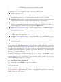
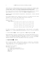
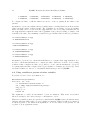
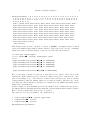
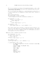
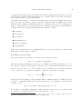
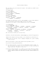
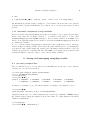
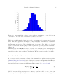
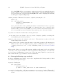
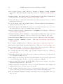
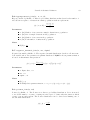
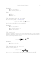
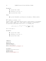
You can examine the marginal posterior of any variable by plotting a histogram of its trace:
>>> from pylab import hist, show
>>> hist(M.trace('l')[:])
(array([
8,
52, 565, 1624, 2563, 2105, 1292, 488, 258,
45]),
array([ 0.52721865, 0.60788251, 0.68854637, 0.76921023, 0.84987409,
0.93053795, 1.01120181, 1.09186567, 1.17252953, 1.25319339]),
<a list of 10 Patch objects>)
>>> show()
You should see something similar to Figure 3.
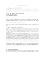
PyMC has its own plotting functionality, via the optional matplotlib module as noted in the
installation notes. The Matplot module includes a plot function that takes the model (or a
single parameter) as an argument:
>>> from pymc.Matplot import plot
>>> plot(M)
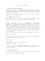
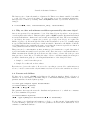
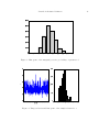
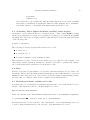
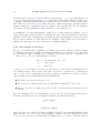
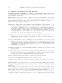
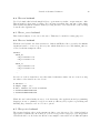
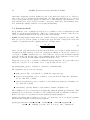
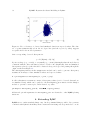
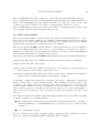
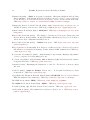
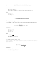
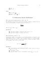
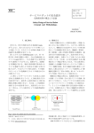
For each variable in the model, plot generates a composite figure, such as that for the
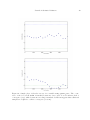
switchpoint in the disasters model (Figure 4). The left-hand pane of this figure shows the
temporal series of the samples from s, while the right-hand pane shows a histogram of the
trace. The trace is useful for evaluating and diagnosing the algorithm’s performance (see
Gelman, Carlin, Stern, and Rubin (2004)), while the histogram is useful for visualizing the
posterior.
For a non-graphical summary of the posterior, simply call M.stats().
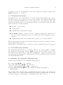
3.11. Imputation of missing data
As with most “textbook examples”, the models we have examined so far assume that the
associated data are complete. That is, there are no missing values corresponding to any
observations in the dataset. However, many real-world datasets contain one or more missing
values, usually due to some logistical problem during the data collection process. The easiest
way of dealing with observations that contain missing values is simply to exclude them from
1
Note that the unknown variables s, e, l and r will all accrue samples, but D will not because its value has
been observed and is not updated. Hence D has no trace and calling M.trace(’D’)[:] will raise an error.
Journal of Statistical Software
15
3000
2500
2000
1500
1000
500
00.5
0.6
0.7
0.8
0.9
1.0
1.1
1.2
1.3
1.4
Figure 3: Histogram of the marginal posterior probability of parameter l.
55
2000
50
1500
s
Frequency
45
1000
40
500
35
300 1000 2000 3000 4000 5000 6000 7000 8000 9000
Iteration
030
35
40
s
45
50
Figure 4: Temporal series and histogram of the samples drawn for s.
55
16
PyMC: Bayesian Stochastic Modelling in Python
Count
15
10
6
Site
1
1
1
Observer
1
2
1
Temperature
15
NA
11
Table 1: Survey dataset for some wildlife species.
the analysis. However, this results in loss of information if an excluded observation contains
valid values for other quantities, and can bias results. An alternative is to impute the missing
values, based on information in the rest of the model.
For example, consider a survey dataset for some wildlife species in Table 1. Each row contains
the number of individuals seen during the survey, along with three covariates: the site on which
the survey was conducted, the observer that collected the data, and the temperature during
the survey. If we are interested in modelling, say, population size as a function of the count
and the associated covariates, it is difficult to accommodate the second observation because
the temperature is missing (perhaps the thermometer was broken that day). Ignoring this
observation will allow us to fit the model, but it wastes information that is contained in the
other covariates.
In a Bayesian modelling framework, missing data are accommodated simply by treating them
as unknown model parameters. Values for the missing data ỹ are estimated naturally, using
the posterior predictive distribution:
Z
p(ỹ|y) =
p(ỹ|θ)f (θ|y)dθ
(2)
This describes additional data ỹ, which may either be considered unobserved data or potential
future observations. We can use the posterior predictive distribution to model the likely values
of missing data, which accounts for both predictive and inferential uncertainty.
Consider the coal mining disasters data introduced previously. Assume that two years of data
are missing from the time series; we indicate this in the data array by the use of an arbitrary
placeholder value, None.
x = numpy.array([
3, 3, 5, 4, 5, 3,
2, 2, 3, 4, 2, 1,
1, 0, 1, 1, 0, 0,
0, 1, 0, 1, 0, 0,
3, 3, 1, None, 2,
0, 0, 0, 1, 0, 0,
4,
1,
3,
3,
0,
1,
0,
5, 4,
4, 4,
None,
1, 0,
2, 1,
1, 1,
0, 0,
0,
1,
2,
3,
0,
1,
1,
1,
5,
1,
2,
0,
2,
0,
4,
5,
1,
2,
0,
4,
0,
3,
3,
1,
0,
1,
2,
1,
4,
4,
1,
1,
1,
0,
0,
0, 6, 3, 3, 4, 0, 2, 6,
2, 5,
3, 0, 0,
1, 1,
0, 2,
0, 1, 4,
1])
To estimate these values in PyMC, we generate a masked array. These are specialised NumPy
arrays that contain a matching True or False value for each element to indicate if that value
should be excluded from any computation. Masked arrays can be generated using NumPy’s
ma.masked_equal function:
>>> masked_data = numpy.ma.masked_equal(x, value=None)
>>> masked_data
Journal of Statistical Software
17
masked_array(data = [4 5 4 0 1 4 3 4 0 6 3 3 4 0 2 6 3 3 5 4 5 3 1 4 4 1 5 5
3 4 2 5 2 2 3 4 2 1 3 -- 2 1 1 1 1 3 0 0 1 0 1 1 0 0 3 1 0 3 2 2 0 1 1 1 0
1 0 1 0 0 0 2 1 0 0 0 1 1 0 2 3 3 1 -- 2 1 1 1 1 2 4 2 0 0 1 4 0 0 0 1 0 0
0 0 0 1 0 0 1 0 1],
mask = [False False False False False False False False False False False
False False False False False False False False False False False False
False False False False False False False False False False False False
False False False False True False False False False False False False
False False False False False False False False False False False False
False False False False False False False False False False False False
False False False False False False False False False False False False
True False False False False False False False False False False False
False False False False False False False False False False False False
False False False False],
fill_value=?)
This masked array, in turn, can then be passed to PyMC’s own Impute function, which
replaces the missing values with Stochastic variables of the desired type. For the coal mining
disasters problem, recall that disaster events were modelled as Poisson variates:
>>> from pymc import Impute
>>> D = Impute('D', Poisson,
>>> D
[<pymc.distributions.Poisson
<pymc.distributions.Poisson
<pymc.distributions.Poisson
<pymc.distributions.Poisson
...
<pymc.distributions.Poisson
masked_data, mu=r)
'D[0]'
'D[1]'
'D[2]'
'D[3]'
at
at
at
at
0x4ba42d0>,
0x4ba4330>,
0x4ba44d0>,
0x4ba45f0>,
'D[110]' at 0x4ba46d0>]
Here r is an array of means for each year of data, allocated according to the location of the
switchpoint. Each element in D is a Poisson Stochastic, irrespective of whether the observation was missing or not. The difference is that actual observations are data Stochastics
(observed=True), while the missing values are non-data Stochastics. The latter are considered unknown, rather than fixed, and therefore estimated by the MCMC algorithm, just as
unknown model parameters.
In this example, we have manually generated the masked array for illustration. In practice,
the Impute function will mask arrays automatically, replacing all None values with Stochastics.
Hence, only the original data array needs to be passed.
The entire model looks very similar to the original model:
s = DiscreteUniform('s', lower=0, upper=110)
e = Exponential('e', beta=1)
l = Exponential('l', beta=1)
@deterministic(plot=False)
18
PyMC: Bayesian Stochastic Modelling in Python
7
400
6
350
300
5
250
D[83]
Frequency
4
3
150
2
100
1
00
200
50
200
400
600
Iteration
800
1000
00
1
2
3
D[83]
4
5
6
7
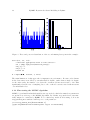
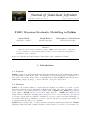
Figure 5: Trace and posterior distribution of the second missing data point in the example.
def r(s=s, e=e, l=l):
"""Allocate appropriate mean to time series"""
out = numpy.empty(len(disasters_array))
out[:s] = e
out[s:] = l
return out
D = Impute('D', Poisson, x, mu=r)
The main limitation of this approach for imputation is performance. Because each element
in the data array is modelled by an individual Stochastic, rather than a single Stochastic
for the entire array, the number of nodes in the overall model increases from 4 to 113. This
significantly slows the rate of sampling, due to the overhead costs associated with iterations
over individual nodes.
3.12. Fine-tuning the MCMC algorithm
MCMC objects handle individual variables via step methods, which determine how parameters
are updated at each step of the MCMC algorithm. By default, step methods are automatically assigned to variables by PyMC. To see which step methods M is using, look at its
step_method_dict attribute with respect to each parameter:
>>> M.step_method_dict[DisasterModel.s]
[<pymc.StepMethods.DiscreteMetropolis object at 0x3e8cb50>]
Journal of Statistical Software
19
>>> M.step_method_dict[DisasterModel.e]
[<pymc.StepMethods.Metropolis object at 0x3e8cbb0>]
>>> M.step_method_dict[DisasterModel.l]
[<pymc.StepMethods.Metropolis object at 0x3e8ccb0>]
The value of step_method_dict corresponding to a particular variable is a list of the step
methods M is using to handle that variable.
You can force M to use a particular step method by calling M.use_step_method before telling
it to sample. The following call will cause M to handle l with a standard Metropolis step
method, but with proposal standard deviation equal to 2:
>>> from pymc import Metropolis
M.use_step_method(Metropolis, DisasterModel.l, proposal_sd=2.)
Another step method class, AdaptiveMetropolis, is better at handling highly-correlated
variables. If your model mixes poorly, using AdaptiveMetropolis is a sensible first thing to
try.
3.13. Beyond the basics
That was a brief introduction to basic PyMC usage. Many more topics are covered in the
subsequent sections, including:
ˆ Class Potential, another building block for probability models in addition to Stochastic
and Deterministic
ˆ Normal approximations
ˆ Using custom probability distributions
ˆ Object architecture
ˆ Saving traces to the disk, or streaming them to the disk during sampling
ˆ Writing your own step methods and fitting algorithms.
Also, be sure to check out the documentation for the Gaussian process extension, which is
available on PyMC’s download page at http://code.google.com/p/pymc/downloads/list.
4. Building models
Bayesian inference begins with specification of a probability model relating unknown variables
to data. PyMC provides three basic building blocks for probability models: Stochastic,
Deterministic and Potential.
A Stochastic object represents a variable whose value is not completely determined by its
parents, and a Deterministic object represents a variable that is entirely determined by its
20
PyMC: Bayesian Stochastic Modelling in Python
parents. Stochastic and Deterministic are subclasses of the Variable class, which only
serves as a template for other classes and is never actually implemented in models.
The third basic class, Potential, represents ‘factor potentials’ (Lauritzen, Dawid, Larsen,
and Leimer 1990; Jordan 2004), which are not variables but simply terms and/or constraints
that are multiplied into joint distributions to modify them. Potential and Variable are
subclasses of Node.
PyMC probability models are simply linked groups of Stochastic, Deterministic and
Potential objects. These objects have very limited awareness of the models in which they
are embedded and do not themselves possess methods for updating their values in fitting
algorithms. Objects responsible for fitting probability models are described in Section 5.
4.1. The Stochastic class
A stochastic variable has the following primary attributes:
value: The variable’s current value.
logp: The log-probability of the variable’s current value given the values of its parents.
A stochastic variable can optionally be endowed with a method called rand, which draws a
value for the variable given the values of its parents2 . Stochastic variables have the following
additional attributes:
parents: A dictionary containing the variable’s parents. The keys of the dictionary are to
the labels assigned to the parents by the variable, and the values correspond to the
actual parents. For example, the keys of s’s parents dictionary in model (1) would be
‘t_l’ and ‘t_h’. The actual parents (i.e., the values of the dictionary) may be of any
class or type.
children: A set containing the variable’s children.
extended_parents: A set containing all stochastic variables on which the variable depends,
either directly or via a sequence of deterministic variables. If the value of any of these
variables changes, the variable will need to recompute its log-probability.
extended_children: A set containing all stochastic variables and potentials that depend on
the variable, either directly or via a sequence of deterministic variables. If the variable’s
value changes, all of these variables and potentials will need to recompute their logprobabilities.
observed: A flag (boolean) indicating whether the variable’s value has been observed (is
fixed).
dtype: A NumPy dtype object (such as numpy.int) that specifies the type of the variable’s
value. The variable’s value is always cast to this type. If this is None (default) then no
type is enforced.
2
Note that the random method does not provide a Gibbs sample unless the variable has no children.
Journal of Statistical Software
21
4.2. Creation of stochastic variables
There are three main ways to create stochastic variables, called the automatic, decorator, and
direct interfaces.
Automatic Stochastic variables with standard distributions provided by PyMC (see Appendix) can be created in a single line using special subclasses of Stochastic. For
example, the uniformly-distributed discrete variable s in (1) could be created using the
automatic interface as follows:
import pymc as pm
s = pm.DiscreteUniform('s', 1851, 1962, value=1900)
In addition to the classes in the appendix, scipy.stats.distributions’ random variable classes are wrapped as Stochastic subclasses if SciPy is installed. These distributions are in the submodule pymc.SciPyDistributions.
Users can call the class factory stochastic_from_dist to produce Stochastic subclasses of their own from probability distributions not included with PyMC.
Decorator Uniformly-distributed discrete stochastic variable s in (1) could alternatively be
created from a function that computes its log-probability as follows:
@pm.stochastic(dtype=int)
def s(value=1900, t_l=1851, t_h=1962):
"""The switchpoint for the rate of disaster occurrence."""
if value > t_h or value < t_l:
return -numpy.inf
else:
return -numpy.log(t_h - t_l + 1)
Note that this is a simple Python function preceded by a Python expression called a
decorator (van Rossum 2010), here called @stochastic. Generally, decorators enhance
functions with additional properties or functionality. The Stochastic object produced
by the @stochastic decorator will evaluate its log-probability using the function s.
The value argument, which is required, provides an initial value for the variable. The
remaining arguments will be assigned as parents of s (i.e., they will populate the parents
dictionary).
To emphasize, the Python function decorated by @stochastic should compute the logdensity or log-probability of the variable. That’s why the return value in the example
above is − log(th − tl + 1) rather than 1/(th − tl + 1).
The value and parents of stochastic variables may be any objects, provided the logprobability function returns a real number (float). PyMC and SciPy both provide
implementations of several standard probability distributions that may be helpful for
creating custom stochastic variables. Based on informal comparison using version 2.0,
the distributions in PyMC tend to be approximately an order of magnitude faster than
their counterparts in SciPy (using version 0.7). See the PyMC wiki page on benchmarks
at http://code.google.com/p/pymc/wiki/Benchmarks.
22
PyMC: Bayesian Stochastic Modelling in Python
The decorator stochastic can take any of the arguments Stochastic.__init__ takes
except parents, logp, random, doc and value. These arguments include trace, plot,
verbose, dtype, rseed and name.
The decorator interface has a slightly more complex implementation which allows you
to specify a random method for sampling the stochastic variable’s value conditional on
its parents.
@pm.stochastic(dtype=int)
def s(value=1900, t_l=1851, t_h=1962):
"""The switchpoint for the rate of disaster occurrence."""
def logp(value, t_l, t_h):
if value > t_h or value < t_l:
return -numpy.inf
else:
return -numpy.log(t_h - t_l + 1)
def random(t_l, t_h):
return numpy.round( (t_l - t_h) * random() ) + t_l
The stochastic variable again gets its name, docstring and parents from function s, but
in this case it will evaluate its log-probability using the logp function. The random
function will be used when s.random() is called. Note that random doesn’t take a
value argument, as it generates values itself.
Direct It’s possible to instantiate Stochastic directly:
def s_logp(value, t_l, t_h):
if value > t_h or value < t_l:
return -numpy.inf
else:
return -numpy.log(t_h - t_l + 1)
def s_rand(t_l, t_h):
return numpy.round( (t_l - t_h) * random() ) + t_l
s = pm.Stochastic( logp = s_logp,
doc = 'The switchpoint for the rate of disaster occurrence.',
name = 's',
parents = {`t_l': 1851, 't_h': 1962},
random = s_rand,
trace = True,
value = 1900,
dtype=int,
rseed = 1.,
observed = False,
cache_depth = 2,
Journal of Statistical Software
23
plot=True,
verbose = 0)
Notice that the log-probability and random variate functions are specified externally
and passed to Stochastic as arguments. This is a rather awkward way to instantiate
a stochastic variable; consequently, such implementations should be rare.
4.3. A warning: Don’t update stochastic variables’ values in-place
Stochastic objects’ values should not be updated in-place. This confuses PyMC’s caching
scheme and corrupts the process used for accepting or rejecting proposed values in the MCMC
algorithm. The only way a stochastic variable’s value should be updated is using statements
of the following form:
A.value = new_value
The following are in-place updates and should never be used:
ˆ A.value += 3
ˆ A.value[2,1] = 5
ˆ A.value.attribute = new_attribute_value.
This restriction becomes onerous if a step method proposes values for the elements of an
array-valued variable separately. In this case, it may be preferable to partition the variable
into several scalar-valued variables stored in an array or list.
4.4. Data
Data are represented by Stochastic objects whose observed attribute is set to True. Although the data are modelled with statistical distributions, their values should be treated as
immutable (since they have been observed). If a stochastic variable’s observed flag is True,
its value cannot be changed, and it won’t be sampled by the fitting method.
4.5. Declaring stochastic variables to be data
In each interface, an optional keyword argument observed can be set to True. In the decorator
interface, this argument is added to the @stochastic decorator:
@pm.stochastic(observed=True)
In the other interfaces, the observed=True argument is added to the initialization arguments:
x = pm.Binomial('x', value=7, n=10, p=.8, observed=True)
Alternatively, in the decorator interface only, a Stochastic object’s observed flag can be set
to true by using an @observed decorator in place of the @stochastic decorator:
24
PyMC: Bayesian Stochastic Modelling in Python
@observed(dtype=int)
def ...
4.6. The Deterministic class
The Deterministic class represents variables whose values are completely determined by the
values of their parents. For example, in model (1), r is a deterministic variable. Recall it
was defined by
e t≤s
rt =
,
l t>s
so r’s value can be computed exactly from the values of its parents e, l and s.
A deterministic variable’s most important attribute is value, which gives the current value
of the variable given the values of its parents. Like Stochastic’s logp attribute, this attribute
is computed on-demand and cached for efficiency.
A Deterministic variable has the following additional attributes:
parents: A dictionary containing the variable’s parents. The keys of the dictionary correspond to the labels assigned to the parents, and the values correspond to the actual
parents.
children: A set containing the variable’s children, which must be nodes (variables or potentials).
Deterministic variables have no methods.
4.7. Creation of deterministic variables
There are several ways to create deterministic variables:
Automatic A handful of common functions have been wrapped in Deterministic subclasses.
These are brief enough to list:
LinearCombination: Has two parents x and y, both of which must be iterable (i.e.,
vector-valued). The value of a linear combination is
X
xTi yi .
i
Index: Has two parents x and index. x must be iterable, index must be valued as an
integer. The value of an index is
x[index].
Index is useful for implementing dynamic models, in which the parent-child connections change.
Lambda: Converts an anonymous function (in Python, called lambda functions) to a
Deterministic instance on a single line.
Journal of Statistical Software
25
CompletedDirichlet: PyMC represents Dirichlet variables of length k by the first k −1
elements; since they must sum to 1, the k−th element is determined by the others.
CompletedDirichlet appends the k−th element to the value of its parent D.
Logit, InvLogit, StukelLogit, StukelInvLogit: Two common link functions for generalized linear models and their inverses.
It’s a good idea to use these classes when feasible in order to give hints to step methods.
Elementary operations on variables Certain elementary operations on variables create
deterministic variables. For example:
>>> x = pm.MvNormalCov('x',numpy.ones(3),numpy.eye(3))
>>> y = pm.MvNormalCov('y',numpy.ones(3),numpy.eye(3))
>>> print x+y
<pymc.PyMCObjects.Deterministic '(x_add_y)' at 0x105c3bd10>
>>> print x[0]
<pymc.CommonDeterministics.Index 'x[0]' at 0x105c52390>
>>> print x[1]+y[2]
<pymc.PyMCObjects.Deterministic '(x[1]_add_y[2])' at 0x105c52410>
All the objects thus created have trace=False and plot=False by default. This convenient method of generating simple deterministics was inspired by Kerman and Gelman
(2004).
Decorator A deterministic variable can be created via a decorator in a way very similar to
Stochastic’s decorator interface:
@pm.deterministic
def r(switchpoint = s, early_rate = e, late_rate = l):
"""The rate of disaster occurrence."""
value = numpy.zeros(len(D))
value[:switchpoint] = early_rate
value[switchpoint:] = late_rate
return value
Notice that rather than returning the log-probability, as is the case for Stochastic
objects, the function returns the value of the deterministic object, given its parents.
This return value may be of any type, as is suitable for the problem at hand. Also
notice that, unlike for Stochastic objects, there is no value argument passed, since
the value is calculated deterministically by the function itself. Arguments’ keys and
values are converted into a parent dictionary as with Stochastic’s short interface.
The deterministic decorator can take trace, verbose and plot arguments, like the
stochastic decorator3 .
Direct Deterministic can also be instantiated directly:
3
Note that deterministic variables have no observed flag. If a deterministic variable’s value were known,
its parents would be restricted to the inverse image of that value under the deterministic variable’s evaluation
function. This usage would be extremely difficult to support in general, but it can be implemented for particular
applications at the StepMethod level.
26
PyMC: Bayesian Stochastic Modelling in Python
def r_eval(switchpoint = s, early_rate = e, late_rate = l):
value = numpy.zeros(len(D))
value[:switchpoint] = early_rate
value[switchpoint:] = late_rate
return value
r = pm.Deterministic(eval = r_eval,
name = 'r',
parents = {`switchpoint': s, 'early_rate': e, 'late_rate': l},
doc = 'The rate of disaster occurrence.',
trace = True,
verbose = 0,
dtype=float,
plot=False,
cache_depth = 2)
4.8. Containers
In some situations it would be inconvenient to assign a unique label to each parent of a
variable. Consider y in the following model:
x0 ∼ N(0, τx )
xi+1 |xi ∼ N(xi , τx )
y|x ∼ N
N
−1
X
i = 0, . . . , N − 2
!
x2i , τy
i=0
Here, y depends on every element of the Markov chain x, but we wouldn’t want to manually
enter N parent labels ‘x_0’, ‘x_1’, etc.
This situation can be handled easily in PyMC:
N = 10
x_0 = pm.Normal('x_0', mu=0, tau=1)
x = numpy.empty(N, dtype=object)
x[0] = x_0
for i in range(1,N):
x[i] = pm.Normal('x_%i' % i, mu=x[i-1], tau=1)
@pm.observed
def y(value = 1, mu = x, tau = 100):
return pm.normal_like(value, numpy.sum(mu**2), tau)
PyMC automatically wraps array x in an appropriate Container class. The expression
‘x_%i’%i labels each Normal object in the container with the appropriate index i; so if
i=1, the name of the corresponding element becomes ‘x_1’.
Journal of Statistical Software
27
Containers, like variables, have an attribute called value. This attribute returns a copy of the
(possibly nested) iterable that was passed into the container function, but with each variable
inside replaced with its corresponding value.
Containers can currently be constructed from lists, tuples, dictionaries, Numpy arrays, modules, sets or any object with a __dict__ attribute. Variables and non-variables can be freely
mixed in these containers, and different types of containers can be nested4 . Containers attempt to behave like the objects they wrap. All containers are subclasses of ContainerBase.
Containers have the following useful attributes in addition to value:
ˆ variables
ˆ stochastics
ˆ potentials
ˆ deterministics
ˆ data_stochastics
ˆ step_methods.
Each of these attributes is a set containing all the objects of each type in a container, and
within any containers in the container.
4.9. The Potential class
The joint density corresponding to model (1) can be written as follows:
p(D, s, l, e) = p(D|s, l, e)p(s)p(l)p(e).
Each factor in the joint distribution is a proper, normalized probability distribution for one of
the variables conditional on its parents. Such factors are contributed by Stochastic objects.
In some cases, it’s nice to be able to modify the joint density by incorporating terms that
don’t correspond to probabilities of variables conditional on parents, for example:
p(x0 , x2 , . . . xN −1 ) ∝
N
−2
Y
ψi (xi , xi+1 ).
i=0
In other cases we may want to add probability terms to existing models. For example, suppose
we want to constrain the difference between e and l in (1) to be less than 1, so that the joint
density becomes
p(D, s, l, e) ∝ p(D|s, l, e)p(s)p(l)p(e)I(|e − l| < 1).
It’s possible to express this constraint by adding variables to the model, or by grouping e and
l to form a vector-valued variable, but it’s uncomfortable to do so.
4
Nodes whose parents are containers make private shallow copies of those containers. This is done for
technical reasons rather than to protect users from accidental misuse.
28
PyMC: Bayesian Stochastic Modelling in Python
Arbitrary factors such as ψ and the indicator function I(|e − l| < 1) are implemented by
objects of class Potential (Lauritzen et al. (1990) and Jordan (2004) call these terms ‘factor
potentials’). Bayesian hierarchical notation (cf model (1)) doesn’t accomodate these potentials. They are often used in cases where there is no natural dependence hierarchy, such as
the first example above (which is known as a Markov random field). They are also useful for
expressing ‘soft data’ (Christakos 2002) as in the second example above.
Potentials have one important attribute, logp, the log of their current probability or probability density value given the values of their parents. The only other attribute of interest is
parents, a dictionary containing the potential’s parents. Potentials have no methods. They
have no trace attribute, because they are not variables. They cannot serve as parents of
variables (for the same reason), so they have no children attribute.
4.10. An example of soft data
The role of potentials can be confusing, so we will provide another example: we have a dataset
t consisting of the days on which several marked animals were recaptured. We believe that
the probability S that an animal is not recaptured on any given day can be explained by a
covariate vector x. We model this situation as follows:
ti |Si ∼ Geometric(Si ), i = 1 . . . N
Si = logit−1 (βxi )
β ∼ N(µβ , Vβ ).
So far, so good. Now suppose we have some knowledge of other related experiments and we
are confident S will be independent of the value of β. It’s not obvious how to work this ‘soft
data’, because as we’ve written the model S is completely determined by β. There are three
options within the strict Bayesian hierarchical framework:
ˆ Work the soft data into the prior on β.
ˆ Incorporate the data from the previous experiments explicitly into the model.
ˆ Refactor the model so that S is at the bottom of the hierarchy, and assign the prior
directly.
Factor potentials provide a convenient way to incorporate the soft data without the need for
such major modifications. We can simply modify the joint distribution from
p(t|S(x, β))p(β)
to
γ(S)p(t|S(x, β))p(β),
where the value of γ is large if S’s value is plausible (based on our external information) and
small otherwise. We do not know the normalizing constant for the new distribution, but we
don’t need it to use most popular fitting algorithms. It’s a good idea to check the induced
Journal of Statistical Software
29
priors on S and β for sanity. This can be done in PyMC by fitting the model with the data
t removed.
It’s important to understand that γ is not a variable, so it does not have a value. That means,
among other things, there will be no γ column in MCMC traces.
4.11. Creation of Potentials
There are two ways to create potentials:
Decorator A potential can be created via a decorator in a way very similar to Deterministic’s
decorator interface:
@pm.potential
def psi_i(x_lo = x[i], x_hi = x[i+1]):
"""A pair potential"""
return -(x_lo - x_hi)**2
The function supplied should return the potential’s current log-probability or log-density
as a NumPy float. The potential decorator can take verbose and cache_depth
arguments like the stochastic decorator.
Direct The same potential could be created directly as follows:
def psi_i_logp(x_lo = x[i], x_hi = x[i+1]):
return -(x_lo - x_hi)**2
psi_i = pm.Potential( logp = psi_i_logp,
name = 'psi_i',
parents = {`xlo': x[i], 'xhi': x[i+1]},
doc = 'A pair potential',
verbose = 0,
cache_depth = 2)
4.12. Graphing models
The function graph (or dag) in pymc.graph draws graphical representations of Model (Section 5) instances using Graphviz via the Python package PyDot. See Lauritzen et al. (1990)
and Jordan (2004) for more discussion of useful information that can be read off of graphical
models. Note that these authors do not consider deterministic variables.
The symbol for stochastic variables is an ellipse. Parent-child relationships are indicated by
arrows. These arrows point from parent to child and are labeled with the names assigned
to the parents by the children. PyMC’s symbol for deterministic variables is a downwardpointing triangle. A graphical representation of model (1) is shown in Figure 2. Note that D
is shaded because it is flagged as data.
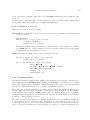
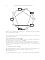
The symbol for factor potentials is a rectangle (Figure 6). Factor potentials are usually associated with undirected grahical models. In undirected representations, each parent of a
potential is connected to every other parent by an undirected edge. The undirected representation of the model is much more compact (Figure 7). Directed or mixed graphical models
30
PyMC: Bayesian Stochastic Modelling in Python
chi
p
d
p
p
c
p
gamma
p
p
p
psi
e
p
p
p
p
p
b
zeta
p
p
phi
p
a
Figure 6: Directed graphical model example. Factor potentials are represented by rectangles
and stochastic variables by ellipses.
can be represented in an undirected form by ‘moralizing’, which is done by the function
pymc.graph.moral_graph.
4.13. Class LazyFunction and caching
This section gives an overview of how PyMC computes log-probabilities. This is advanced
information that is not required in order to use PyMC.
The logp attributes of stochastic variables and potentials and the value attributes of deterministic variables are wrappers for instances of class LazyFunction. Lazy functions are
wrappers for ordinary Python functions. A lazy function L could be created from a function
fun as follows:
L = pm.LazyFunction(fun, arguments)
The argument arguments is a dictionary container; fun must accept keyword arguments only.
When L’s get() method is called, the return value is the same as the call
fun(**arguments.value)
Note that no arguments need to be passed to L.get; lazy functions memorize their arguments.
Journal of Statistical Software
31
e
b
c
d
a
Figure 7: The undirected version of the graphical model of Figure 6.
Before calling fun, L will check the values of its arguments’ extended children against an
internal cache. This comparison is done by reference, not by value, and this is part of the
reason why stochastic variables’ values cannot be updated in-place. If the arguments’ extended
children’s values match a frame of the cache, the corresponding output value is returned and
fun is not called. If a call to fun is needed, the arguments’ extended children’s values and the
return value replace the oldest frame in the cache. The depth of the cache can be set using
the optional init argument cache_depth, which defaults to 2.
Caching is helpful in MCMC, because variables’ log-probabilities and values tend to be queried
multiple times for the same parental value configuration. The default cache depth of 2 turns
out to be most useful in Metropolis-Hastings-type algorithms involving proposed values that
may be rejected.
Lazy functions are implemented in C using Pyrex (Ewing 2010), a language for writing Python
extensions.
5. Fitting models
PyMC provides three objects that fit models:
ˆ MCMC, which coordinates Markov chain Monte Carlo algorithms. The actual work of
updating stochastic variables conditional on the rest of the model is done by StepMethod
objects, which are described in this section.
ˆ MAP, which computes maximum a posteriori estimates.
ˆ NormApprox, which computes the ‘normal approximation’ (Gelman et al. 2004): the
joint distribution of all stochastic variables in a model is approximated as normal using
local information at the maximum a posteriori estimate.
32
PyMC: Bayesian Stochastic Modelling in Python
All three objects are subclasses of Model, which is PyMC’s base class for fitting methods.
MCMC and NormApprox, both of which can produce samples from the posterior, are subclasses
of Sampler, which is PyMC’s base class for Monte Carlo fitting methods. Sampler provides
a generic sampling loop method and database support for storing large sets of joint samples.
These base classes are documented at the end of this section.
5.1. Creating models
The first argument to any fitting method’s init method, including that of MCMC, is called
input. The input argument can be just about anything; once you have defined the nodes
that make up your model, you shouldn’t even have to think about how to wrap them in a
Model instance. Some examples of model instantiation using nodes a, b and c follow:
ˆ M = Model(set([a,b,c]))
ˆ M = Model({‘a’: a, ‘d’: [b,c]}) In this case, M will expose a and d as attributes: M.a will be a, and M.d will be [b,c].
ˆ M = Model([[a,b],c])
ˆ If file MyModule contains the definitions of a, b and c:
import MyModule
M = Model(MyModule)
In this case, M will expose a, b and c as attributes.
ˆ Using a ‘model factory’ function:
def make_model(x):
a = pm.Exponential('a',beta=x,value=0.5)
@pm.deterministic
def b(a=a):
return 100-a
@pm.stochastic
def c(value=0.5, a=a, b=b):
return (value-a)**2/b
return locals()
M = pm.Model(make_model(3))
In this case, M will also expose a, b and c as attributes.
5.2. The Model class
Model serves as a container for probability models and as a base class for the classes responsible
for model fitting, such as MCMC.
Model’s init method takes the following arguments:
Journal of Statistical Software
33
input: Some collection of PyMC nodes defining a probability model. These may be stored
in a list, set, tuple, dictionary, array, module, or any object with a __dict__ attribute.
verbose (optional): An integer controlling the verbosity of the model’s output.
Models’ useful methods are:
draw_from_prior(): Sets all stochastic variables’ values to new random values, which would
be a sample from the joint distribution if all data and Potential instances’ log-probability
functions returned zero. If any stochastic variables lack a random() method, PyMC will
raise an exception.
seed(): Same as draw_from_prior, but only stochastics whose rseed attribute is not
None are changed.
The helper function graph produces graphical representations of models (Jordan 2004, see).
Models have the following important attributes:
ˆ variables
ˆ stochastics
ˆ potentials
ˆ deterministics
ˆ observed_stochastics
ˆ step_methods
ˆ value: A copy of the model, with each attribute that is a PyMC variable or container
replaced by its value.
ˆ generations: A topological sorting of the stochastics in the model.
In addition, models expose each node they contain as an attribute. For instance, if model M
were produced from model (1) M.s would return the switchpoint variable.
5.3. Maximum a posteriori estimates
The MAP class sets all stochastic variables to their maximum a posteriori values using functions in SciPy’s optimize package. SciPy must be installed to use it. MAP can only handle variables whose dtype is float, so it will not work on model 1. To fit the model in
examples/gelman_bioassay.py using MAP, do the following
>>> from pymc.examples import gelman_bioassay
>>> M = pm.MAP(gelman_bioassay)
>>> M.fit()
This call will cause M to fit the model using Nelder-Mead optimization, which does not
require derivatives. The variables in gelman_bioassay have now been set to their maximum
a posteriori values:
34
PyMC: Bayesian Stochastic Modelling in Python
>>> M.alpha.value
array(0.8465892309923545)
>>> M.beta.value
array(7.7488499785334168)
In addition, the AIC and BIC of the model are now available:
>>> M.AIC
7.9648372671389458
>>> M.BIC
6.7374259893787265
MAP has two useful methods:
fit(method =’fmin’, iterlim=1000, tol=.0001): The optimization method may be fmin,
fmin_l_bfgs_b, fmin_ncg, fmin_cg, or fmin_powell. See the documentation of SciPy’s
optimize package for the details of these methods. The tol and iterlim parameters
are passed to the optimization function under the appropriate names.
revert_to_max(): If the values of the constituent stochastic variables change after fitting,
this function will reset them to their maximum a posteriori values.
If you’re going to use an optimization method that requires derivatives, MAP’s init method
can take additional parameters eps and diff_order. diff_order, which must be an integer,
specifies the order of the numerical approximation (see the SciPy function derivative). The
step size for numerical derivatives is controlled by eps, which may be either a single value or
a dictionary of values whose keys are variables (actual objects, not names).
The useful attributes of MAP are:
logp: The joint log-probability of the model.
logp_at_max: The maximum joint log-probability of the model.
AIC: Akaike’s information criterion for this model (Akaike 1973; Burnham and Anderson
2002).
BIC: The Bayesian information criterion for this model (Schwarz 1978).
One use of the MAP class is finding reasonable initial states for MCMC chains. Note that
multiple Model subclasses can handle the same collection of nodes.
5.4. Normal approximations
The NormApprox class extends the MAP class by approximating the posterior covariance of the
model using the Fisher information matrix, or the Hessian of the joint log probability at the
maximum. To fit the model in examples/gelman_bioassay.py using NormApprox, do:
>>> N = pm.NormApprox(gelman_bioassay)
>>> N.fit()
Journal of Statistical Software
35
The approximate joint posterior mean and covariance of the variables are available via the
attributes mu and C:
>>> N.mu[N.alpha]
array([ 0.84658923])
>>> N.mu[N.alpha, N.beta]
array([ 0.84658923, 7.74884998])
>>> N.C[N.alpha]
matrix([[ 1.03854093]])
>>> N.C[N.alpha, N.beta]
matrix([[ 1.03854093,
3.54601911],
[ 3.54601911, 23.74406919]])
As with MAP, the variables have been set to their maximum a posteriori values (which are
also in the mu attribute) and the AIC and BIC of the model are available.
In addition, it’s now possible to generate samples from the posterior as with MCMC:
>>> N.sample(100)
>>> N.trace('alpha')[::10]
array([-0.85001278, 1.58982854, 1.0388088 , 0.07626688, 1.15359581,
-0.25211939, 1.39264616, 0.22551586, 2.69729987, 1.21722872])
>>> N.trace('beta')[::10]
array([ 2.50203663, 14.73815047, 11.32166303,
0.43115426,
10.1182532 ,
7.4063525 , 11.58584317,
8.99331152,
11.04720439,
9.5084239 ])
Any of the database backends can be used (Section 6).
In addition to the methods and attributes of MAP, NormApprox provides the following methods:
sample(iter): Samples from the approximate posterior distribution are drawn and stored.
isample(iter): An ‘interactive’ version of sample(): sampling can be paused, returning
control to the user.
draw: Sets all variables to random values drawn from the approximate posterior.
It provides the following additional attributes:
mu: A special dictionary-like object that can be keyed with multiple variables. N.mu[p1, p2,
p3] would return the approximate posterior mean values of stochastic variables p1, p2
and p3, ravelled and concatenated to form a vector.
C: Another special dictionary-like object. N.C[p1, p2, p3] would return the approximate
posterior covariance matrix of stochastic variables p1, p2 and p3. As with mu, these
variables’ values are ravelled and concatenated before their covariance matrix is constructed.
36
PyMC: Bayesian Stochastic Modelling in Python
5.5. Markov chain Monte Carlo: The MCMC class
The MCMC class implements PyMC’s core business: producing Markov chains from a model’s
variables which can be considered sequences of joint samples from the posterior. See Section 3
for an example of basic usage.
MCMC’s primary job is to create and coordinate a collection of ‘step methods’, each of which
is responsible for updating one or more variables. The available step methods are described
below. Instructions on how to create your own step method are available in Section 8.
MCMC provides the following useful methods:
sample(iter, burn, thin, tune_interval, tune_throughout, save_interval, . . . ):
Runs the MCMC algorithm and produces the traces. The iter argument controls the
total number of MCMC iterations. No tallying will be done during the first burn iterations; these samples will be forgotten. After this burn-in period, tallying will be done
each thin iterations. Tuning will be done each tune_interval iterations. If tune_throughout=False, no more tuning will be done after the burnin period. The model
state will be saved every save_interval iterations, if given.
isample(iter, burn, thin, tune_interval, tune_throughout, save_interval, . . . ):
An interactive version of sample. The sampling loop may be paused at any time, returning control to the user.
use_step_method(method, *args, **kwargs): Creates an instance of step method class
method to handle some stochastic variables. The extra arguments are passed to the
init method of method. Assigning a step method to a variable manually will prevent
the MCMC instance from automatically assigning one. However, you may handle a variable
with multiple step methods.
goodness(): Calculates goodness-of-fit (GOF) statistics according to Brooks, Catchpole, and
Morgan (2000).
save_state(): Saves the current state of the sampler, including all stochastics, to the database.
This allows the sampler to be reconstituted at a later time to resume sampling. This is
not supported yet for the RDBMS backends, sqlite and mysql.
restore_state(): Restores the sampler to the state stored in the database.
stats(): Generates summary statistics for all nodes in the model.
remember(trace_index): Set all variables’ values from frame trace_index in the database.
MCMC samplers’ step methods can be accessed via the step_method_dict attribute.
M.step_method_dict[x] returns a list of the step methods M will use to handle the stochastic
variable x.
After sampling, the information tallied by M can be queried via M.db.trace_names. In addition to the values of variables, tuning information for adaptive step methods is generally
tallied. These ‘traces’ can be plotted to verify that tuning has in fact terminated.
You can produce ‘traces’ for arbitrary functions with zero arguments as well. If you issue the
command M._funs_to_tally[’trace_name’] = f before sampling begins, then each time
Journal of Statistical Software
37
the model variables’ values are tallied f will be called with no arguments, and the return value
will be tallied. After sampling ends you can retrieve the trace as M.trace[’trace_name’]
5.6. The Sampler class
MCMC is a subclass of a more general class called Sampler. Samplers fit models with Monte
Carlo fitting methods, which characterize the posterior distribution by approximate samples
from it. They are initialized as follows: Sampler(input=None, db=’ram’, name=’Sampler’,
reinit_model=True, calc_deviance=False). The input argument is a module, list, tuple,
dictionary, set, or object that contains all elements of the model, the db argument indicates
which database backend should be used to store the samples (see Section 6), reinit_model is
a boolean flag that indicates whether the model should be re-initialised before running, and
calc_deviance is a boolean flag indicating whether deviance should be calculated for the
model at each iteration. Samplers have the following important methods:
sample(iter, length=None, verbose=0): Samples from the joint distribution. The iter
argument controls how many times the sampling loop will be run, and the length
argument controls the initial size of the database that will be used to store the samples.
isample(iter, length=None, verbose=0): The same as sample, but the sampling is done
interactively: you can pause sampling at any point and be returned to the Python
prompt to inspect progress and adjust fitting parameters. While sampling is paused,
the following methods are useful:
icontinue(): Continue interactive sampling.
halt(): Truncate the database and clean up.
tally(): Write all variables’ current values to the database. The actual write operation
depends on the specified database backend.
save_state(): Saves the current state of the sampler, including all stochastics, to the database.
This allows the sampler to be reconstituted at a later time to resume sampling. This is
not supported yet for the RDBMS backends, sqlite and mysql.
restore_state(): Restores the sampler to the state stored in the database.
stats(): Generates summary statistics for all nodes in the model.
remember(trace_index): Set all variables’ values from frame trace_index in the database.
Note that the trace_index is different from the current iteration, since not all samples
are necessarily saved due to burning and thinning.
In addition, the sampler attribute deviance is a deterministic variable valued as the model’s
deviance at its current state.
5.7. Step methods
Step method objects handle individual stochastic variables, or sometimes groups of them.
They are responsible for making the variables they handle take single MCMC steps conditional on the rest of the model. Each subclass of StepMethod implements a method called
38
PyMC: Bayesian Stochastic Modelling in Python
step(), which is called by MCMC. Step methods with adaptive tuning parameters can optionally implement a method called tune(), which causes them to assess performance (based on
the acceptance rates of proposed values for the variable) so far and adjust.
The major subclasses of StepMethod are Metropolis, AdaptiveMetropolis and Gibbs.
PyMC provides several flavors of the basic Metropolis steps, but the Gibbs steps are not
ready for use as of the current release. However, because it is feasible to write Gibbs step
methods for particular applications, the Gibbs base class will be documented here.
5.8. Metropolis step methods
Metropolis and subclasses implement Metropolis-Hastings steps. To tell an MCMC object M
to handle a variable x with a Metropolis step method, you might do the following:
M.use_step_method(pm.Metropolis, x, proposal_sd=1., \
proposal_distribution='Normal')
Metropolis itself handles float-valued variables, and subclasses DiscreteMetropolis and
BinaryMetropolis handle integer- and boolean-valued variables, respectively. Subclasses of
Metropolis must implement the following methods:
propose(): Sets the values of the variables handled by the Metropolis step method to proposed values.
reject(): If the Metropolis-Hastings acceptance test fails, this method is called to reset the
values of the variables to their values before propose() was called.
Note that there is no accept() method; if a proposal is accepted, the variables’ values are simply left alone. Subclasses that use proposal distributions other than symmetric random-walk
may specify the ‘Hastings factor’ by changing the hastings_factor method. See Section 8
for an example.
Metropolis’ init method takes the following arguments:
stochastic: The variable to handle.
proposal_sd: A float or array of floats. This sets the default proposal standard deviation if
the proposal distribution is normal.
scale: A float, defaulting to 1. If the scale argument is provided but not proposal_sd,
proposal_sd is computed as follows:
if all(self.stochastic.value != 0.):
self.proposal_sd = ones(shape(self.stochastic.value)) * \
abs(self.stochastic.value) * scale
else:
self.proposal_sd = ones(shape(self.stochastic.value)) * scale
proposal_distribution: A string indicating which distribution should be used for proposals.
Current options are ‘Normal’ and ‘Prior’. If proposal_distribution=None, the
proposal distribution is chosen automatically. It is set to ‘Prior’ if the variable has no
children and has a random method, and to ‘Normal’ otherwise.
Journal of Statistical Software
39
verbose: An integer. By convention, 0 indicates minimal output and 2 indicates maximum
verbosity.
Although the proposal_sd attribute is fixed at creation, Metropolis step methods adjust this
initial value using an attribute called adaptive_scale_factor. When tune() is called, the
acceptance ratio of the step method is examined and this scale factor is updated accordingly. If
the proposal distribution is normal, proposals will have standard deviation self.proposal_sd
* self.adaptive_scale_factor.
By default, tuning will continue throughout the sampling loop, even after the burnin period
is over. This can be changed via the tune_throughout argument to MCMC.sample. If an
adaptive step method’s tally flag is set (the default for Metropolis), a trace of its tuning
parameters will be kept. If you allow tuning to continue throughout the sampling loop, it is
important to verify that the ‘Diminishing Tuning’ condition of Roberts and Rosenthal (2007)
is satisfied: the amount of tuning should decrease to zero, or tuning should become very
infrequent.
If a Metropolis step method handles an array-valued variable, it proposes all elements independently but simultaneously. That is, it decides whether to accept or reject all elements
together but it does not attempt to take the posterior correlation between elements into account. The AdaptiveMetropolis class (see below), on the other hand, does make correlated
proposals.
5.9. The AdaptiveMetropolis class
The AdaptativeMetropolis (AM) step method works like a regular Metropolis step method,
with the exception that its variables are block-updated using a multivariate jump distribution
whose covariance is tuned during sampling. Although the chain is non-Markovian, it has
correct ergodic properties (see Haario, Saksman, and Tamminen (2001)).
To tell an MCMC object M to handle variables x, y and z with an AdaptiveMetropolis instance,
you might do the following:
M.use_step_method(pm.AdaptiveMetropolis, [x,y,z], \
scales={x:1, y:2, z:.5}, delay=10000)
AdaptativeMetropolis’ init method takes the following arguments:
stochastics: The stochastic variables to handle. These will be updated jointly.
cov (optional): An initial covariance matrix. Defaults to the identity matrix, adjusted according to the scales argument.
delay (optional): The number of iterations to delay before computing the empirical covariance matrix.
scales (optional): The initial covariance matrix will be diagonal, and its diagonal elements
will be set to scales times the stochastics’ values, squared.
interval (optional): The number of iterations between updates of the covariance matrix.
Defaults to 1000.
40
PyMC: Bayesian Stochastic Modelling in Python
greedy (optional): If True, only accepted jumps will be counted toward the delay before
the covariance is first computed. Defaults to True.
verbose (optional): An integer from 0 to 3 controlling the verbosity of the step method’s
printed output.
shrink_if_necessary (optional): Whether the proposal covariance should be shrunk if the
acceptance rate becomes extremely small.
In this algorithm, jumps are proposed from a multivariate normal distribution with covariance
matrix C. The algorithm first iterates until delay samples have been drawn (if greedy is true,
until delay jumps have been accepted). At this point, C is given the value of the empirical
covariance of the trace so far and sampling resumes. The covariance is then updated each
interval iterations throughout the entire sampling run5 . It is this constant adaptation of
the proposal distribution that makes the chain non-Markovian.
5.10. The DiscreteMetropolis class
This class is just like Metropolis, but specialized to handle Stochastic instances with dtype
int. The jump proposal distribution can either be ‘Normal’, ‘Prior’ or ‘Poisson’. In the
normal case, the proposed value is drawn from a normal distribution centered at the current
value and then rounded to the nearest integer. In the Poisson case, the proposed value is
obtained by adding or substracting (with equal probability) a random value drawn from a
Poisson distribution.
5.11. The BinaryMetropolis class
This class is specialized to handle Stochastic instances with dtype bool.
For array-valued variables, BinaryMetropolis can be set to propose from the prior by passing
in dist="Prior". Otherwise, the argument p_jump of the init method specifies how probable a
change is. Like Metropolis’ attribute proposal_sd, p_jump is tuned throughout the sampling
loop via adaptive_scale_factor.
For scalar-valued variables, BinaryMetropolis behaves like a Gibbs sampler, since this requires no additional expense. The p_jump and adaptive_scale_factor parameters are not
used in this case.
5.12. Granularity of step methods: One-at-a-time vs. block updating
There is currently no way for a stochastic variable to compute individual terms of its logprobability; it is computed all together. This means that updating the elements of a arrayvalued variable individually would be inefficient, so all existing step methods update arrayvalued variables together, in a block update.
To update an array-valued variable’s elements individually, simply break it up into an array
of scalar-valued variables. Instead of this:
A = pm.Normal('A', value=numpy.zeros(100), mu=0., tau=1.)
5
The covariance is estimated recursively from the previous value and the last interval samples, instead of
computing it each time from the entire trace.
Journal of Statistical Software
41
do this:
A = [pm.Normal('A_%i'%i, value=0., mu=0., tau=1.) for i in range(100)]
An individual step method will be assigned to each element of A in the latter case, and the
elements will be updated individually. Note that A can be broken up into larger blocks if
desired.
5.13. Automatic assignment of step methods
Every step method subclass (including user-defined ones) that does not require any init arguments other than the stochastic variable to be handled adds itself to a list called
StepMethodRegistry in the PyMC namespace. If a stochastic variable in an MCMC object
has not been explicitly assigned a step method, each class in StepMethodRegistry is allowed
to examine the variable.
To do so, each step method implements a class method called competence, whose only argument is a single stochastic variable. These methods return values from 0 to 3; 0 meaning the
step method cannot safely handle the variable and 3 meaning it will most likely be the best
available step method for variables like this. The MCMC object assigns the step method that
returns the highest competence value to each of its stochastic variables.
6. Saving and managing sampling results
6.1. Accessing sampled data
The recommended way to access data from an MCMC run, irrespective of the database
backend, is to use the trace method:
>>> from pymc.examples import DisasterModel
>>> M = pm.MCMC(DisasterModel)
>>> M.sample(10)
>>> M.trace('e')[:]
array([ 2.28320992, 2.28320992, 2.28320992,
2.36982455, 2.36982455, 3.1669422 ,
2.28320992,
3.1669422 ,
2.28320992,
3.14499489])
M.trace(’e’) returns a copy of the Trace instance belonging to the tallyable object e:
>>> M.trace('e')
<pymc.database.ram.Trace object at 0x7fa4877a8b50>
Samples from the trace are obtained using the slice notation [], similarly to NumPy arrays.
By default, trace returns the samples from the last chain. To return samples from all the
chains, set chain=None:
>>> M.sample(5)
>>> M.trace('e', chain=None)[:]
42
PyMC: Bayesian Stochastic Modelling in Python
array([ 2.28320992,
2.36982455,
3.14499489,
2.28320992,
2.36982455,
3.14499489,
2.28320992,
3.1669422 ,
3.14499489,
2.28320992,
3.1669422 ,
2.94672454,
2.28320992,
3.14499489,
3.10767686])
6.2. Saving data to disk
By default, the database backend selected by the MCMC sampler is the ram backend, which
simply holds the data in RAM. Now, we create a sampler that, instead, writes data to a pickle
file:
>>> M = pm.MCMC(DisasterModel, db='pickle', dbname='Disaster.pickle')
>>> M.db
<pymc.database.pickle.Database object at 0x7fa486623d90>
>>> M.sample(10)
>>> M.db.close()
Note that in this particular case, no data is written to disk before the call to db.close. The
close method will flush data to disk and prepare the database for a potential session exit.
Closing a Python session without calling close beforehand is likely to corrupt the database,
making the data irretrievable. To simply flush data to disk without closing the database, use
the commit method.
Some backends not only have the ability to store the traces, but also the state of the step
methods at the end of sampling. This is particularly useful when long warm-up periods are
needed to tune the jump parameters. When the database is loaded in a new session, the step
methods query the database to fetch the state they were in at the end of the last trace.
Check that you close the database before closing the Python session.
6.3. Loading back a database
To load a file created in a previous session, use the load function from the appropriate
backend:
>>> db = pymc.database.pickle.load('Disaster.pickle')
>>> len(db.trace('e')[:])
10
The db object also has a trace method identical to that of Sampler. You can hence inspect
the results of a model, even if you don’t have the model around.
To add a new trace to this file, we need to create an MCMC instance. This time, instead
of setting db=’pickle’, we will pass the existing Database instance and sample as usual. A
new trace will be appended to the first:
>>>
>>>
>>>
15
>>>
M = MCMC(DisasterModel, db=db)
M.sample(5)
len(M.trace('e', chain=None)[:])
M.db.close()
Journal of Statistical Software
43
6.4. The ram backend
Used by default, this backend simply holds a copy in memory, with no output written to disk.
This is useful for short runs or testing. For long runs generating large amount of data, using
this backend may fill the available memory, forcing the OS to store data in the cache, slowing
down all other applications.
6.5. The no_trace backend
This backend simply does not store the trace. This may be useful for testing purposes.
6.6. The txt backend
With the txt backend, the data is written to disk in ASCII files. More precisely, the dbname
argument is used to create a top directory into which chain directories, called Chain_<#>, are
created each time sample is called:
dbname/
Chain_0/
<object0
<object1
...
Chain_1/
<object0
<object1
...
...
name>.txt
name>.txt
name>.txt
name>.txt
In each one of these chain directories, files named <variable name>.txt are created, storing
the values of the variable as rows of text:
# Variable: e
# Sample shape: (5,)
# Date: 2008-11-18 17:19:13.554188
3.033672373807017486e+00
3.033672373807017486e+00
...
While the txt backend makes it easy to load data using other applications and programming
languages, it is not optimized for speed nor memory efficiency. If you plan on generating and
handling large datasets, read on for better options.
6.7. The pickle backend
The pickle database relies on the cPickle module to save the traces. Use of this backend is
appropriate for small scale, short-lived projects. For longer term or larger projects, the pickle
backend should be avoided since the files it creates might be unreadable across different Python
44
PyMC: Bayesian Stochastic Modelling in Python
versions. The pickled file is a simple dump of a dictionary containing the NumPy arrays
storing the traces, as well as the state of the Sampler’s step methods.
6.8. The sqlite backend
The sqlite backend is based on the python module sqlite3 (a Python 2.5 built-in) . It
opens an SQL database named dbname, and creates one table per tallyable objects. The rows
of this table store a key, the chain index and the values of the objects:
key (INT), trace (INT),
v1 (FLOAT), v2 (FLOAT), v3 (FLOAT) ...
The key is autoincremented each time a new row is added to the table, that is, each time
tally is called by the sampler. Note that the savestate feature is not implemented, that is,
the state of the step methods is not stored internally in the database.
6.9. The mysql backend
The mysql backend depends on the MySQL library and its python wrapper MySQLdb (Dustman 2010). Like the sqlite backend, it creates an SQL database containing one table per
tallyable object. The main difference with sqlite is that it can connect to a remote database,
provided the url and port of the host server is given, along with a valid user name and password. These parameters are passed when the Sampler is instantiated:
ˆ dbname The name of the database file.
ˆ dbuser The database user name.
ˆ dbpass The user password for this database.
ˆ dbhost The location of the database host.
ˆ dbport The port number to use to reach the database host.
ˆ dbmode File mode. Use a to append values, and w to overwrite an existing database.
The savestate feature is not implemented in the mysql backend.
6.10. The hdf5 backend
The hdf5 backend uses PyTables to save data in binary HDF5 format. The hdf5 database is
fast and can store huge traces, far larger than the available RAM. Data can be compressed and
decompressed on the fly to reduce the disk footprint. Another feature of this backend is that
it can store arbitrary objects. Whereas most of the other backends are limited to numerical
values, hdf5 can tally any object that can be pickled, opening the door for powerful and
exotic applications (see pymc.gp).
The internal structure of an HDF5 file storing both numerical values and arbitrary objects is
as follows:
/ (root)
/chain0/ (Group) 'Chain #0'
Journal of Statistical Software
45
/chain0/PyMCSamples (Table(N,)) 'PyMC Samples'
/chain0/group0 (Group) 'Group storing objects.'
/chain0/group0/<object0 name> (VLArray(N,)) '<object0 name> samples.'
/chain0/group0/<object1 name> (VLArray(N,)) '<object1 name> samples.'
...
/chain1/ (Group) 'Chain \#1'
...
All standard numerical values are stored in a Table, while objects are stored in individual
VLArrays.
The hdf5 Database takes the following parameters:
ˆ dbname Name of the hdf5 file.
ˆ dbmode File mode: a: append, w: overwrite, r: read-only.
ˆ dbcomplevel: Compression level, 0: no compression, 9: maximal compression.
ˆ dbcomplib Compression library (zlib, bzip2, LZO)
According the the PyTables manual, zlib Roelofs, loup Gailly, and Adler (2010) has a fast
decompression, relatively slow compression, and a good compression ratio; LZO Oberhumer
(2008) has a fast compression, but a low compression ratio; and bzip2 Seward (2007) has
an excellent compression ratio but requires more CPU. Note that some of these compression
algorithms require additional software to work (see the PyTables manual).
6.11. Writing a new backend
It is relatively easy to write a new backend for PyMC. The first step is to look at the
database.base module, which defines barebone Database and Trace classes. This module
contains documentation on the methods that should be defined to get a working backend.
Testing your new backend should be fairly straightforward, since the test_database module
contains a generic test class that can easily be subclassed to check that the basic features
required of all backends are implemented and working properly.
7. Model checking and diagnostics
7.1. Convergence diagnostics
Valid inferences from sequences of MCMC samples are based on the assumption that samples
are derived from the true posterior distribution of interest. Theory guarantees this condition
as the number of iterations approaches infinity. It is important, therefore, to determine the
minimum number of samples required to ensure a reasonable approximation to the target
posterior density. Unfortunately, no universal threshold exists across all problems, so convergence must be assessed independently each time MCMC estimation is performed. The
procedures for verifying convergence are collectively known as convergence diagnostics.
46
PyMC: Bayesian Stochastic Modelling in Python
Figure 8: An example of a poorly-mixing sample in two dimensions. Notice that the chain is
trapped in a region of low probability relative to the mean (dot) and variance (oval) of the
true posterior quantity.
One approach to analyzing convergence is analytical, whereby the variance of the sample
at different sections of the chain are compared to that of the limiting distribution. These
methods use distance metrics to analyze convergence, or place theoretical bounds on the
sample variance, and though they are promising, they are generally difficult to use and are
not prominent in the MCMC literature. More common is a statistical approach to assessing
convergence. Statistical techniques, rather than considering the properties of the theoretical
target distribution, only consider the statistical properties of the observed chain. Reliance
on the sample alone restricts such convergence criteria to heuristics, and hence, convergence
cannot be guaranteed. Although evidence for lack of convergence using statistical convergence
diagnostics will correctly imply lack of convergence in the chain, the absence of such evidence
will not guarantee convergence in the chain. Nevertheless, negative results for one or more
criteria will provide some measure of assurance to users that their sample will provide valid
inferences.
For most simple models, convergence will occur quickly, sometimes within the first several
hundred iterations, after which all remaining samples of the chain may be used to calculate
posterior quantities. For many more complex models, convergence requires a significantly
longer burn-in period; sometimes orders of magnitude more samples are needed. Frequently,
lack of convergence will be caused by poor mixing (Figure 8). Mixing refers to the degree to
which the Markov chain explores the support of the posterior distribution. Poor mixing may
stem from inappropriate proposals (if one is using the Metropolis-Hastings sampler) or from
attempting to estimate models with highly correlated variables.
7.2. Informal methods
The most straightforward approach for assessing convergence is based on simply plotting and
Journal of Statistical Software
47
Figure 9: An example of metastability in a two-dimensional parameter space. The chain
appears to be stable in one region of the parameter space for an extended period, then
unpredictably jumps to another region of the space.
inspecting traces and histograms of the observed MCMC sample. If the trace of values for
each of the stochastics exhibits asymptotic behaviour6 over the last m iterations, this may be
satisfactory evidence for convergence. A similar approach involves plotting a histogram for
every set of k iterations (perhaps 50-100) beyond some burn-in threshold n; if the histograms
are not visibly different among the sample intervals, this is some evidence for convergence.
Note that such diagnostics should be carried out for each stochastic estimated by the MCMC
algorithm, because convergent behaviour by one variable does not imply evidence for convergence for other variables in the model. An extension of this approach can be taken when
multiple parallel chains are run, rather than just a single, long chain. In this case, the final
values of c chains run for n iterations are plotted in a histogram; just as above, this is repeated every k iterations thereafter, and the histograms of the endpoints are plotted again
and compared to the previous histogram. This is repeated until consecutive histograms are
indistinguishable.
Another ad hoc method for detecting convergence is to examine the traces of several MCMC
chains initialized with different starting values. Overlaying these traces on the same set of axes
should (if convergence has occurred) show each chain tending toward the same equilibrium
value, with approximately the same variance. Recall that the tendency for some Markov
chains to converge to the true (unknown) value from diverse initial values is called ergodicity.
This property is guaranteed by the reversible chains constructed using MCMC, and should
be observable using this technique. Again, however, this approach is only a heuristic method,
and cannot always detect lack of convergence, even though chains may appear ergodic.
A principal reason that evidence from informal techniques cannot guarantee convergence is a
phenomenon called metastability. Chains may appear to have converged to the true equilib6
Asymptotic behaviour implies that the variance and the mean value of the sample stays relatively constant
over some arbitrary period.
48
PyMC: Bayesian Stochastic Modelling in Python
rium value, displaying excellent qualities by any of the methods described above. However,
after some period of stability around this value, the chain may suddenly move to another
region of the parameter space (Figure 9). This period of metastability can sometimes be very
long, and therefore escape detection by these convergence diagnostics. Unfortunately, there
is no statistical technique available for detecting metastability.
7.3. Formal methods
Along with the ad hoc techniques described above, a number of more formal methods exist
which are prevalent in the literature. These are considered more formal because they are
based on existing statistical methods, such as time series analysis.
PyMC currently includes functions for two formal convergence diagnostic procedures. The
first, proposed by Geweke (1992), is a time-series approach that compares the mean and
variance of segments from the beginning and end of a single chain.
z=p
θ̄a − θ̄b
V ar(θa ) + V ar(θb )
(3)
where a is the early interval and b the late interval. If the z-scores (theoretically distributed
as standard normal variates) of these two segments are similar, it can provide evidence for
convergence. PyMC calculates z-scores of the difference between various initial segments
along the chain, and the last 50% of the remaining chain. If the chain has converged, the
majority of points should fall within 2 standard deviations of zero.
Diagnostic z-scores can be obtained by calling the geweke function. It accepts either (1) a
single trace, (2) a Node or Stochastic object, or (3) an entire Model object:
pm.geweke(pymc_object, first=0.1, last=0.5, intervals=20)
The arguments expected are the following
ˆ pymc_object: The object that is or contains the output trace(s).
ˆ first (optional): First portion of chain to be used in Geweke diagnostic. Defaults to
0.1 (i.e., first 10% of chain).
ˆ last (optional): Last portion of chain to be used in Geweke diagnostic. Defaults to 0.5
(i.e., last 50% of chain).
ˆ intervals (optional): Number of sub-chains to analyze. Defaults to 20.
The resulting scores are best interpreted graphically, using the geweke_plot function. This
displays the scores in series, in relation to the 2 standard deviation boundaries around zero.
Hence, it is easy to see departures from the standard normal assumption.
geweke_plot takes either a single set of scores, or a dictionary of scores (output by geweke
when an entire Sampler is passed) as its argument:
geweke_plot(scores, name='geweke', format='png', suffix='-diagnostic', \
path='./', fontmap = {1:10, 2:8, 3:6, 4:5, 5:4}, verbose=1)
Journal of Statistical Software
49
Figure 10: Sample plots of Geweke z-scores for a variable using geweke_plot. The occurrence of the scores well within 2 standard deviations of zero gives does not indicate lack of
convergence (top), while deviations exceeding 2 standard deviations suggests that additional
samples are required to achieve convergence (bottom).
50
PyMC: Bayesian Stochastic Modelling in Python
ˆ scores: The object that contains the Geweke scores. Can be a list (one set) or a
dictionary (multiple sets).
ˆ name (optional): Name used for output files. For multiple scores, the dictionary keys
are used as names.
ˆ format (optional): Graphic output file format (defaults to png).
ˆ suffix (optional): Suffix to filename (defaults to -diagnostic)
ˆ path (optional): The path for output graphics (defaults to working directory).
ˆ fontmap (optional): Dictionary containing the font map for the labels of the graphic.
ˆ verbose (optional): Verbosity level for output (defaults to 1).
To illustrate, consider a model my_model that is used to instantiate a MCMC sampler. The
sampler is then run for a given number of iterations:
>>> S = pm.MCMC(my_model)
>>> S.sample(10000, burn=5000)
It is easiest simply to pass the entire sampler S to the geweke function:
>>> scores = pm.geweke(S, intervals=20)
>>> pm.Matplot.geweke_plot(scores)
Alternatively, individual stochastics within S can be analyzed for convergence:
>>> trace = S.trace('alpha')[:]
>>> alpha_scores = pm.geweke(trace, intervals=20)
>>> pm.Matplot.geweke_plot(alpha_scores, 'alpha')
An example of convergence and non-convergence of a chain using geweke_plot is given in
Figure 10.
The second diagnostic provided by PyMC is the Raftery and Lewis (1995a) procedure. This
approach estimates the number of iterations required to reach convergence, along with the
number of burn-in samples to be discarded and the appropriate thinning interval. A separate
estimate of both quantities can be obtained for each variable in a given model.
As the criterion for determining convergence, the Raftery and Lewis approach uses the accuracy of estimation of a user-specified quantile. For example, we may want to estimate the
quantile q = 0.975 to within r = 0.005 with probability s = 0.95. In other words,
P r(|q̂ − q| ≤ r) = s
(4)
From any sample of θ, one can construct a binary chain:
Z (j) = I(θ(j) ≤ uq )
(5)
Journal of Statistical Software
51
where uq is the quantile value and I is the indicator function. While {θ(j) } is a Markov chain,
{Z (j) } is not necessarily so. In any case, the serial dependency among Z (j) decreases as the
thinning interval k increases. A value of k is chosen to be the smallest value such that the
first order Markov chain is preferable to the second order Markov chain.
This thinned sample is used to determine number of burn-in samples. This is done by comparing the remaining samples from burn-in intervals of increasing length to the limiting distribution of the chain. An appropriate value is one for which the truncated sample’s distribution
is within (arbitrarily small) of the limiting distribution. See Raftery and Lewis (1995a) or
Gamerman (1997) for computational details. Estimates for sample size tend to be conservative.
This diagnostic is best used on a short pilot run of a particular model, and the results used
to parameterize a subsequent sample that is to be used for inference. Its calling convention
is as follows:
raftery_lewis(pymc_object, q, r, s=.95, epsilon=.001, verbose=1)
The arguments are:
ˆ pymc_object: The object that contains the Geweke scores. Can be a list (one set) or a
dictionary (multiple sets).
ˆ q: Desired quantile to be estimated.
ˆ r: Desired accuracy for quantile.
ˆ s (optional): Probability of attaining the requested accuracy (defaults to 0.95).
ˆ epsilon (optional): Half width of the tolerance interval required for the q-quantile
(defaults to 0.001).
ˆ verbose (optional): Verbosity level for output (defaults to 1).
The code for raftery_lewis is based on the Fortran program gibbsit (Raftery and Lewis
1995b).
For example, consider again a sampler S run for some model my_model:
>>> S = pm.MCMC(my_model)
>>> S.sample(10000, burn=5000)
One can pass either the entire sampler S or any stochastic within S to the raftery_lewis
function, along with suitable arguments. Here, we have chosen q = 0.025 (the lower limit of
the equal-tailed 95% interval) and error r = 0.01:
>>> pm.raftery_lewis(S, q=0.025, r=0.01)
This yields diagnostics as follows for each stochastic of S, as well as a dictionary containing
the diagnostic quantities:
52
PyMC: Bayesian Stochastic Modelling in Python
========================
Raftery-Lewis Diagnostic
========================
937 iterations required (assuming independence) to achieve 0.01 accuracy
with 95 percent probability.
Thinning factor of 1 required to produce a first-order Markov chain.
39 iterations to be discarded at the beginning of the simulation (burn-in).
11380 subsequent iterations required.
Thinning factor of 11 required to produce an independence chain.
Additional convergence diagnostics are available in the R language (R Development Core
Team 2010), via the coda package (Plummer, Best, Cowles, and Vines 2008). PyMC includes
a method coda for exporting model traces in a format that may be directly read by coda:
pm.utils.coda(pymc_object)
The lone argument is the PyMC sampler for which output is desired.
Calling coda yields two files, one containing raw trace values (suffix .out) and another containing indices to the trace values (suffix .ind).
7.4. Autocorrelation plots
Samples from MCMC algorithms are ususally autocorrelated, due partly to the inherent
Markovian dependence structure. The degree of autocorrelation can be quantified using the
autocorrelation function:
ρk =
=
Cov(Xt , Xt+k )
p
Var(Xt )Var(Xt+k )
E[(Xt − θ)(Xt+k − θ)]
p
E[(Xt − θ)2 ]E[(Xt+k − θ)2 ]
PyMC includes a function for plotting the autocorrelation function for each stochastic in the
sampler (Figure 11). This allows users to examine the relationship among successive samples
within sampled chains. Significant autocorrelation suggests that chains require thinning prior
to use of the posterior statistics for inference.
autocorrelation(pymc_object, name, maxlag=100, format='png', suffix='-acf',
path='./', fontmap = {1:10, 2:8, 3:6, 4:5, 5:4}, verbose=1)
ˆ pymc_object: The object that is or contains the output trace(s).
ˆ name: Name used for output files.
Journal of Statistical Software
53
Figure 11: Sample autocorrelation plots for two Poisson variables from coal mining disasters
example model.
ˆ maxlag: The highest lag interval for which autocorrelation is calculated.
ˆ format (optional): Graphic output file format (defaults to png).
ˆ suffix (optional): Suffix to filename (defaults to -diagnostic)
ˆ path (optional): The path for output graphics (defaults to working directory).
ˆ fontmap (optional): Dictionary containing the font map for the labels of the graphic.
ˆ verbose (optional): Verbosity level for output (defaults to 1).
Using any given model my_model as an example, autocorrelation plots can be obtained simply
by passing the sampler for that model to the autocorrelation function (within the Matplot
module) directly:
>>> S = pm.MCMC(my_model)
>>> S.sample(10000, burn=5000)
>>> pm.Matplot.autocorrelation(S)
Alternatively, variables within a model can be plotted individually. For example, a hypothetical variable beta that was estimated using sampler S will yield a correlation plot as
follows:
>>> pm.Matplot.autocorrelation(S.beta)
54
PyMC: Bayesian Stochastic Modelling in Python
7.5. Goodness of fit
Checking for model convergence is only the first step in the evaluation of MCMC model
outputs. It is possible for an entirely unsuitable model to converge, so additional steps are
needed to ensure that the estimated model adequately fits the data. One intuitive way for
evaluating model fit is to compare model predictions with actual observations. In other
words, the fitted model can be used to simulate data, and the distribution of the simulated
data should resemble the distribution of the actual data.
Fortunately, simulating data from the model is a natural component of the Bayesian modelling
framework. Recall, from the discussion on imputation of missing data, the posterior predictive
distribution:
Z
p(ỹ|y) =
p(ỹ|θ)f (θ|y)dθ
(6)
Here, ỹ represents some hypothetical new data that would be expected, taking into account
the posterior uncertainty in the model parameters. Sampling from the posterior predictive
distribution is easy in PyMC. The code looks identical to the corresponding data stochastic,
with two modifications: (1) the node should be specified as deterministic and (2) the statistical
likelihoods should be replaced by random number generators. As an example, consider a
simple dose-response model, where deaths are modeled as a binomial random variable for
which the probability of death is a logit-linear function of the dose of a particular drug:
n = [5]*4
dose = [-.86,-.3,-.05,.73]
x = [0,1,3,5]
alpha = pm.Normal('alpha', mu=0.0, tau=0.01)
beta = pm.Normal('beta', mu=0.0, tau=0.01)
@pm.deterministic
def theta(a=alpha, b=beta, d=dose):
"""theta = inv_logit(a+b)"""
return pm.invlogit(a+b*d)
"""deaths ~ binomial(n, p)"""
deaths = pm.Binomial('deaths', n=n, p=theta, value=x, observed=True)
The posterior predictive distribution of deaths uses the same functional form as the data
likelihood, in this case a binomial stochastic. Here is the corresponding sample from the
posterior predictive distribution:
@pm.deterministic
def deaths_sim(n=n, p=theta):
"""deaths_sim = rbinomial(n, p)"""
return pm.rbinomial(n, p)
Notice that the stochastic pm.Binomial has been replaced with a deterministic node that
simulates values using pm.rbinomial and the unknown parameters theta.
Journal of Statistical Software
55
Figure 12: Data sampled from the posterior predictive distribution of a model for some
observation x. The true value of x is shown by the dotted red line.
The degree to which simulated data correspond to observations can be evaluated in at least two
ways. First, these quantities can simply be compared visually. This allows for a qualitative
comparison of model-based replicates and observations. If there is poor fit, the true value of
the data may appear in the tails of the histogram of replicated data, while a good fit will
tend to show the true data in high-probability regions of the posterior predictive distribution
(Figure 12).
The Matplot module in PyMC provides an easy way of producing such plots, via the gof_plot
function. To illustrate, consider a single observed data point x and an array of values x_sim
sampled from the posterior predictive distribution. The histogram is generated by calling:
pm.Matplot.gof_plot(x_sim, x, name='x')
A second approach for evaluating goodness of fit using samples from the posterior predictive
distribution involves the use of a statistical criterion. For example, the Bayesian p value
(Gelman, Meng, and Stern 1996) uses a discrepancy measure that quantifies the difference
between data (observed or simulated) x and the expected value e, conditional on some model.
One such discrepancy measure is the Freeman-Tukey statistic (Brooks et al. 2000):
D(x|θ) =
X√
√
( xj − ej )2
(7)
j
Model fit is assessed by comparing the discrepancies from observed data to those from simulated data. On average, we expect the difference between them to be zero; hence, the
Bayesian p value is simply the proportion of simulated discrepancies that are larger than
56
PyMC: Bayesian Stochastic Modelling in Python
Figure 13: Plot of deviates of observed and simulated data from expected values. The cluster of points symmetrically about the 45 degree line (and the reported p value) suggests
acceptable fit for the modeled parameter.
their corresponding observed discrepancies:
p = P r[D(sim) > D(obs)]
(8)
If p is very large (e.g., > 0.975) or very small (e.g., < 0.025) this implies that the model is not
consistent with the data, and thus is evidence of lack of fit. Graphically, data and simulated
discrepancies plotted together should be clustered along a 45 degree line passing through the
origin, as shown in Figure 13.
The discrepancy function in the diagnostics module can be used to generate discrepancy
statistics from arrays of data, simulated values, and expected values:
D = pm.diagnostics.discrepancy(x, x_sim, x_exp)
A call to this function returns two arrays of discrepancy values (one for observed data and one
for simulated data), which can be passed to the discrepancy_plot function in the Matplot
module to generate a scatter plot, and if desired, a p value:
pm.Matplot.discrepancy_plot(D, name='D', report_p=True)
Additional optional arguments for discrepancy_plot are identical to other PyMC plotting
functions.
8. Extending PyMC
PyMC tries to make standard things easy, but keep unusual things possible. Its openness,
combined with Python’s flexibility, invite extensions from using new step methods to exotic
Journal of Statistical Software
57
stochastic processes (see the Gaussian process module). This section briefly reviews the ways
PyMC is designed to be extended.
8.1. Nonstandard stochastics
The simplest way to create a Stochastic object with a nonstandard distribution is to use the
medium or long decorator syntax. See Section 4. If you want to create many stochastics with
the same nonstandard distribution, the decorator syntax can become cumbersome. An actual
subclass of Stochastic can be created using the class factory stochastic_from_dist. This
function takes the following arguments:
ˆ The name of the new class,
ˆ A logp function,
ˆ A random function (which may be None),
ˆ The NumPy datatype of the new class (for continuous distributions, this should be
float; for discrete distributions, int; for variables valued as non-numerical objects,
object),
ˆ A flag indicating whether the resulting class represents a vector-valued variable.
The necessary parent labels are read from the logp function, and a docstring for the new
class is automatically generated.
Full subclasses of Stochastic may be necessary to provide nonstandard behaviors (see gp.GP).
8.2. User-defined step methods
The StepMethod class is meant to be subclassed. There are an enormous number of MCMC
step methods in the literature, whereas PyMC provides only about half a dozen. Most
user-defined step methods will be either Metropolis-Hastings or Gibbs step methods, and
these should subclass Metropolis or Gibbs respectively. More unusual step methods should
subclass StepMethod directly.
8.3. Example: An asymmetric Metropolis step
Consider the probability model in examples/custom_step.py:
mu = pymc.Normal('mu',0,.01, value=0)
tau = pymc.Exponential('tau',.01, value=1)
cutoff = pymc.Exponential('cutoff',1, value=1.3)
D = pymc.TruncatedNormal('D',mu,tau,-numpy.inf,cutoff,value=data, \
observed=True)
The stochastic variable cutoff cannot be smaller than the largest element of D, otherwise D’s
density would be zero. The standard Metropolis step method can handle this case without
problems; it will propose illegal values occasionally, but these will be rejected.
58
PyMC: Bayesian Stochastic Modelling in Python
Suppose we want to handle cutoff with a smarter step method that doesn’t propose illegal
values. Specifically, we want to use the nonsymmetric proposal distribution
xp |x ∼ Truncnorm(x, σ, max(D), ∞).
We can implement this Metropolis-Hastings algorithm with the following step method class:
class TruncatedMetropolis(pymc.Metropolis):
def __init__(self, stochastic, low_bound, up_bound, *args, **kwargs):
self.low_bound = low_bound
self.up_bound = up_bound
pymc.Metropolis.__init__(self, stochastic, *args, **kwargs)
def propose(self):
tau = 1./(self.adaptive_scale_factor * self.proposal_sd)**2
self.stochastic.value = \
pymc.rtruncnorm(self.stochastic.value, tau, self.low_bound, \
self.up_bound)
def hastings_factor(self):
tau = 1./(self.adaptive_scale_factor * self.proposal_sd)**2
cur_val = self.stochastic.value
last_val = self.stochastic.last_value
lp_for = pymc.truncnorm_like(cur_val, last_val, tau, \
self.low_bound, self.up_bound)
lp_bak = pymc.truncnorm_like(last_val, cur_val, tau, \
self.low_bound, self.up_bound)
if self.verbose > 1:
print self._id + ': Hastings factor %f'%(lp_bak - lp_for)
return lp_bak - lp_for
The propose method sets the step method’s stochastic’s value to a new value, drawn from
a truncated normal distribution. The precision of this distribution is computed from two
factors: self.proposal_sd, which can be set with an input argument to Metropolis, and
self.adaptive_scale_factor. Metropolis step methods’ default tuning behavior is to reduce adaptive_scale_factor if the acceptance rate is too low, and to increase
adaptive_scale_factor if it is too high. By incorporating adaptive_scale_factor into
the proposal standard deviation, we avoid having to write our own tuning infrastructure. If
we don’t want the proposal to tune, we don’t have to use adaptive_scale_factor.
The hastings_factor method adjusts for the asymmetric proposal distribution (Gelman
et al. 2004). It computes the log of the quotient of the ‘backward’ density and the ‘forward’
density. For symmetric proposal distributions, this quotient is 1, so its log is zero.
Having created our custom step method, we need to tell MCMC instances to use it to handle
the variable cutoff. This is done in custom_step.py with the following line:
M.use_step_method(TruncatedMetropolis, cutoff, D.value.max(), numpy.inf)
Journal of Statistical Software
59
This call causes M to pass the arguments cutoff, D.value.max(), numpy.inf to a
TruncatedMetropolis object’s init method, and use the object to handle cutoff.
It’s often convenient to get a handle to a custom step method instance directly for debugging
purposes. M.step_method_dict[cutoff] returns a list of all the step methods M will use to
handle cutoff:
>>> M.step_method_dict[cutoff]
[<custom_step.TruncatedMetropolis object at 0x3c91130>]
There may be more than one, and conversely step methods may handle more than one stochastic variable. To see which variables step method S is handling, try
>>> S.stochastics
set([<pymc.distributions.Exponential 'cutoff' at 0x3cd6b90>])
8.4. General step methods
All step methods must implement the following methods:
step(): Updates the values of self.stochastics.
tune(): Tunes the jumping strategy based on performance so far. A default method is
available that increases self.adaptive_scale_factor (see below) when acceptance
rate is high, and decreases it when acceptance rate is low. This method should return
True if additional tuning will be required later, and False otherwise.
competence(s): A class method that examines stochastic variable s and returns a value from
0 to 3 expressing the step method’s ability to handle the variable. This method is used
by MCMC instances when automatically assigning step methods. Conventions are:
0 I cannot safely handle this variable.
1 I can handle the variable about as well as the standard Metropolis step method.
2 I can do better than Metropolis.
3 I am the best step method you are likely to find for this variable in most cases.
For example, if you write a step method that can handle NewStochasticSubclass well,
the competence method might look like this:
class NewStepMethod(pymc.StepMethod):
def __init__(self, stochastic, *args, **kwargs):
...
@classmethod
def competence(self, stochastic):
if isinstance(stochastic, NewStochasticSubclass):
return 3
else:
return 0
60
PyMC: Bayesian Stochastic Modelling in Python
Note that PyMC will not even attempt to assign a step method automatically if its init
method cannot be called with a single stochastic instance, that is NewStepMethod(x) is
a legal call. The list of step methods that PyMC will consider assigning automatically
is called pymc.StepMethodRegistry.
current_state(): This method is easiest to explain by showing the code:
state = {}
for s in self._state:
state[s] = getattr(self, s)
return state
self._state should be a list containing the names of the attributes needed to reproduce
the current jumping strategy. If an MCMC object writes its state out to a database, these
attributes will be preserved. If an MCMC object restores its state from that database later,
the corresponding step method will have these attributes set to their saved values.
Step methods should also maintain the following attributes:
_id: A string that can identify each step method uniquely (usually something like
<class_name>_<stochastic_name>).
adaptive_scale_factor: An ‘adaptive scale factor’. This attribute is only needed if the
default tune() method is used.
_tuning_info: A list of strings giving the names of any tuning parameters. For Metropolis
instances, this would be [‘adaptive_scale_factor’]. This list is used to keep traces
of tuning parameters in order to verify ‘diminishing tuning’ (Roberts and Rosenthal
2007).
All step methods have a property called loglike, which gives the sum of the log-probabilities
of the union of the extended children of self.stochastics. This quantity is one term in the
log of the Metropolis-Hastings acceptance ratio. The logp_plus_loglike property gives the
sum of that and the log-probabilities of self.stochastics.
8.5. Metropolis-Hastings step methods
A Metropolis-Hastings step method only needs to implement the following methods, which
are called by Metropolis.step():
reject(): Usually just
def reject(self):
self.rejected += 1
[s.value = s.last_value for s in self.stochastics]
propose(): Sets the values of all self.stochastics to new, proposed values. This method
may use the adaptive_scale_factor attribute to take advantage of the standard tuning
scheme.
Journal of Statistical Software
61
Metropolis-Hastings step methods may also override the tune and competence methods.
Metropolis-Hastings step methods with asymmetric jumping distributions must implement a
method called hastings_factor(), which returns the log of the ratio of the ‘reverse’ and
‘forward’ proposal probabilities. Note that no accept() method is needed or used.
Metropolis-Hastings step methods should log the number of jumps they have accepted and
rejected using attributes called accepted and rejected.
8.6. Gibbs step methods
Gibbs step methods handle conjugate submodels. These models usually have two components: the ‘parent’ and the ‘children’. For example, a gamma-distributed variable serving as
the precision of several normally-distributed variables is a conjugate submodel; the gamma
variable is the parent and the normal variables are the children.
This section describes PyMC’s current scheme for Gibbs step methods, several of which are
in a semi-working state in the sandbox directory. It is meant to be as generic as possible to
minimize code duplication, but it is admittedly complicated. Feel free to subclass StepMethod
directly when writing Gibbs step methods if you prefer.
Gibbs step methods that subclass PyMC’s Gibbs should define the following class attributes:
child_class: The class of the children in the submodels the step method can handle.
parent_class: The class of the parent.
parent_label: The label the children would apply to the parent in a conjugate submodel.
In the gamma-normal example, this would be tau.
linear_OK: A flag indicating whether the children can use linear combinations involving the
parent as their actual parent without destroying the conjugacy.
A subclass of Gibbs that defines these attributes only needs to implement a propose()
method, which will be called by Gibbs.step(). The resulting step method will be able
to handle both conjugate and ‘non-conjugate’ cases. The conjugate case corresponds to an
actual conjugate submodel. In the nonconjugate case all the children are of the required
class, but the parent is not. In this case the parent’s value is proposed from the likelihood
and accepted based on its prior. The acceptance rate in the nonconjugate case will be less
than one.
The inherited class method Gibbs.competence will determine the new step method’s ability
to handle a variable x by checking whether:
ˆ all x’s children are of class child_class, and either apply parent_label to x directly or
(if linear_OK=True) to a LinearCombination object (Section 4), one of whose parents
contains x.
ˆ x is of class parent_class
If both conditions are met, pymc.conjugate_Gibbs_competence will be returned. If only the
first is met, pymc.nonconjugate_Gibbs_competence will be returned.
62
PyMC: Bayesian Stochastic Modelling in Python
8.7. New fitting algorithms
PyMC provides a convenient platform for non-MCMC fitting algorithms in addition to MCMC.
All fitting algorithms should be implemented by subclasses of Model. There are virtually no
restrictions on fitting algorithms, but many of Model’s behaviors may be useful. See Section 5.
8.8. Monte Carlo fitting algorithms
Unless there is a good reason to do otherwise, Monte Carlo fitting algorithms should be
implemented by subclasses of Sampler to take advantage of the interactive sampling feature
and database backends. Subclasses using the standard sample() and isample() methods
must define one of two methods:
draw(): If it is possible to generate an independent sample from the posterior at every iteration, the draw method should do so. The default _loop method can be used in this
case.
_loop(): If it is not possible to implement a draw() method, but you want to take advantage of the interactive sampling option, you should override _loop(). This method
is responsible for generating the posterior samples and calling tally() when it is appropriate to save the model’s state. In addition, _loop should monitor the sampler’s
status attribute at every iteration and respond appropriately. The possible values of
status are:
‘ready’: Ready to sample.
‘running’: Sampling should continue as normal.
‘halt’: Sampling should halt as soon as possible. _loop should call the halt() method
and return control. _loop can set the status to ‘halt’ itself if appropriate (eg the
database is full or a KeyboardInterrupt has been caught).
‘paused’: Sampling should pause as soon as possible. _loop should return, but should
be able to pick up where it left off next time it’s called.
Samplers may alternatively want to override the default sample() method. In that case, they
should call the tally() method whenever it is appropriate to save the current model state.
Like custom _loop() methods, custom sample() methods should handle KeyboardInterrupts
and call the halt() method when sampling terminates to finalize the traces.
8.9. A second warning: Don’t update stochastic variables’ values in-place
If you’re going to implement a new step method, fitting algorithm or unusual (non-numericvalued) Stochastic subclass, you should understand the issues related to in-place updates of
Stochastic objects’ values. Fitting methods should never update variables’ values in-place
for two reasons:
ˆ In algorithms that involve accepting and rejecting proposals, the ‘pre-proposal’ value
needs to be preserved uncorrupted. It would be possible to make a copy of the preproposal value and then allow in-place updates, but in PyMC we have chosen to store
the pre-proposal value as Stochastic.last_value and require proposed values to be
Journal of Statistical Software
63
new objects. In-place updates would corrupt Stochastic.last_value, and this would
cause problems.
ˆ LazyFunction’s caching scheme checks variables’ current values against its internal
cache by reference. That means if you update a variable’s value in-place, it or its child
may miss the update and incorrectly skip recomputing its value or log-probability.
However, a Stochastic object’s value can make in-place updates to itself if the updates
don’t change its identity. For example, the Stochastic subclass gp.GP is valued as a
gp.Realization object. These represent random functions, which are infinite-dimensional
stochastic processes, as literally as possible. The strategy they employ is to ‘self-discover’ on
demand: when they are evaluated, they generate the required value conditional on previous
evaluations and then make an internal note of it. This is an in-place update, but it is done
to provide the same interface as a single random function whose value everywhere has been
determined since it was created.
9. Conclusion
MCMC is a surprisingly difficult and bug-prone algorithm to implement by hand. We find
PyMC makes it much easier and less stressful. PyMC also makes our work more dynamic;
getting hand-coded MCMC’s working used to be so much work that we were reluctant to
change anything, but with PyMC changing models is much easier.
We welcome new contributors at all levels. If you would like to contribute new code, improve
documentation, share your results or provide ideas for new features, please introduce yourself
on our mailing list at [email protected]. Our wiki page at http://code.google.com/
p/pymc/w/list also hosts a number of tutorials and examples from users that could give you
some ideas. We have taken great care to make the code easy to extend, whether by adding
new database backends, step methods or entirely new sampling algorithms.
Acknowledgments
The authors would like to thank several users of PyMC who have been particularly helpful
during the development of the 2.0 release. In alphabetical order, these are Mike Conroy,
Abraham Flaxman, J. Miguel Marin, Aaron MacNeil, Nick Matsakis, John Salvatier and
Andrew Straw.
Anand Patil’s work on PyMC has been supported since 2008 by the Malaria Atlas Project,
principally funded by the Wellcome Trust.
David Huard’s early work on PyMC was supported by a scholarship from the Natural Sciences
and Engineering Research Council of Canada.
References
Akaike H (1973). “Information Theory as an Extension of the Maximum Likelihood Principle.”
In BN Petrov, F Csaki (eds.), Second International Symposium on Information Theory, pp.
267–281. Akademiai Kiado, Budapest.
64
PyMC: Bayesian Stochastic Modelling in Python
Alted F, Vilata I, Prater S, Mas V, Hedley T, Valentino A, Whitaker J (2010). “PyTables
User’s Guide: Hierarchical Datasets in Python – Release 2.2.” URL http://www.pytables.
org/.
Azzalini A (2010). “The Skew-Normal Probability Distribution (and Related Distributions,
such as the Skew-t).” URL http://azzalini.stat.unipd.it/SN/.
Bernardo JM, Berger J, Dawid AP, Smith JFM (eds.) (1992). Bayesian Statistics 4. Oxford
University Press, Oxford.
Brooks SP, Catchpole EA, Morgan BJT (2000). “Bayesian Animal Survival Estimation.”
Statistical Science, 15, 357–376.
Burnham KP, Anderson DR (2002). Model Selection and Multi-Model Inference: A Practical,
Information-Theoretic Approach. Springer-Verlag, New York.
Carrera E, Theune C (2010). “Python Interface to Graphviz’s Dot Language.” URL http:
//code.google.com/p/pydot/.
Christakos G (2002). “On the Assimilation of Uncertain Physical Knowledge Bases: Bayesian
and Non-Bayesian Techniques.” Advances in Water Resources, 25(8-12), 1257–1274.
Daumé III H (2007). HBC: Hierarchical Bayes Compiler. URL http://hal3.name/HBC/.
Dustman JA (2010). “MySQL for Python.” URL http://sourceforge.net/projects/
mysql-python/.
Eby PJ (2010). “setuptools 0.6c11.” URL http://pypi.python.org/pypi/setuptools/.
Enthought, Inc (2010). “Enthought Python Distribution.” URL http://www.enthought.com/.
Ewing G (2010). Pyrex – A Language for Writing Python Extension Modules. URL http:
//www.cosc.canterbury.ac.nz/greg.ewing/python/Pyrex/.
Free Software Foundation, Inc (2010). “gcc, the GNU Compiler Collection.” URL http:
//gcc.gnu.org/.
Gamerman D (1997). Markov Chain Monte Carlo: Statistical Simulation for Bayesian Inference. Chapman and Hall, London.
Gansner ER, North SC (1999). “An Open Graph Visualization System and Its Applications
to Software Engineering.” Software – Practice and Experience, 00(S1), 1–5.
Gelman A, Carlin JB, Stern HS, Rubin DB (2004). Bayesian Data Analysis. 2nd edition.
Chapman and Hall/CRC, Boca Raton, FL.
Gelman A, Meng XL, Stern H (1996). “Posterior Predictive Assessment of Model Fitness via
Realized Discrepencies.” Statistica Sinica, 6, 733–807.
Geweke J (1992). Evaluating the Accuracy of Sampling-Based Approaches to Calculating
Posterior Moments, pp. 169–193. In Bernardo, Berger, Dawid, and Smith (1992).
Haario H, Saksman E, Tamminen J (2001). “An Adaptive Metropolis Algorithm.” Bernoulli,
7(2), 223–242.
Journal of Statistical Software
65
Hadfield JD (2010). “MCMC Methods for Multi-Response Generalized Linear Mixed Models:
The MCMCglmm R Package.” Journal of Statistical Software, 33(2), 1–22. URL http:
//www.jstatsoft.org/v33/i02/.
Hunter JD (2007). “matplotlib: A 2D Graphics Environment.” Computing in Science &
Engineering, 9(3), 90–95. doi:10.1109/MCSE.2007.55.
Jarrett RG (1979). “A Note on the Intervals Between Coal Mining Disasters.” Biometrika,
66, 191–193.
Jaynes ET (2003). Probability Theory: The Logic of Science. Cambridge University Press,
Cambridge.
Jones E, Oliphant T, Peterson P (2001). “SciPy: Open Source Scientific Tools for Python.”
URL http://www.scipy.org/.
Jordan MI (2004). “Graphical Models.” Statistical Science, 19(1), 140–155.
Kerman J, Gelman A (2004). Fully Bayesian Computing. URL http://stat.columbia.edu/
~gelman/research/unpublished/fullybayesiancomputing-nonblinded.pdf.
Langtangen HP (2009). Python Scripting for Computational Science. Springer-Verlag, Heidelberg.
Lauritzen SL, Dawid AP, Larsen BN, Leimer HG (1990). “Independence Properties of Directed
Markov Fields.” Networks, 20, 491–505.
Lunn D, Thomas A, Best NG, Spiegelhalter DJ (2000). “WinBUGS – A Bayesian Modelling
Framework: Concepts, Structure, and Extensibility.” Statistics and Computing, 10, 325–
337.
Lutz M (2007). Learning Python. O’Reilly Media, Inc., Sebastopol.
Martin AD, Quinn KM, Park JH (2009). MCMCpack: Markov Chain Monte Carlo (MCMC)
Package. R package version 1.0-4, URL http://CRAN.R-project.org/package=MCMCpack.
Oberhumer MFXJ (2008). “LZO Real-Time Data Compression Library.” URL http://www.
oberhumer.com/opensource/lzo/.
Oliphant TE (2006). Guide to NumPy. Provo, UT. URL http://www.tramy.us/.
Oracle Corporation (2010). “MySQL: The World’s Most Popular Open Source Database.”
URL http://www.mysql.com/.
Pellerin J (2010). “nose Is Nicer Testing for Python.” URL http://somethingaboutorange.
com/mrl/projects/nose/.
Pérez F, Granger BE (2007). “IPython: a System for Interactive Scientific Computing.”
Computing in Science and Engineering, 9(3), 21–29.
Peters C (2010). “MinGW: Minimalist GNU for Windows.” URL http://www.mingw.org/.
66
PyMC: Bayesian Stochastic Modelling in Python
Plummer M (2003). “JAGS: A Program for Analysis of Bayesian Graphical Models Using
Gibbs Sampling.” In K Hornik, F Leisch, A Zeileis (eds.), Proceedings of the 3rd International Workshop on Distributed Statistical Computing, Vienna, Austria. ISSN 1609-395X,
URL http://www.ci.tuwien.ac.at/Conferences/DSC-2003/Proceedings/.
Plummer M, Best N, Cowles K, Vines K (2008). coda: Output Analysis and Diagnostics for
MCMC. R package version 0.13-3, URL http://CRAN.R-project.org/package=coda.
Python Software Foundation (2005). “MacPython.” URL http://homepages.cwi.nl/~jack/
macpython/.
Raftery AE, Lewis SM (1995a). “The Number of Iterations, Convergence Diagnostics and
Generic Metropolis Algorithms.” In DJS W R Gilks, S Richardson (eds.), Practical Markov
Chain Monte Carlo. Chapman and Hall, London.
Raftery AE, Lewis SM (1995b). “Gibbsit Version 2.0.” URL http://lib.stat.cmu.edu/
general/gibbsit/.
R Development Core Team (2010). R: A Language and Environment for Statistical Computing.
R Foundation for Statistical Computing, Vienna, Austria. ISBN 3-900051-07-0, URL http:
//www.R-project.org/.
Roberts GO, Rosenthal JS (2007). “Implementing Componentwise Hastings Algorithms.”
Journal of Applied Probability, 44(2), 458–475.
Roelofs G, loup Gailly J, Adler M (2010). “zlib: A Massively Spiffy Yet Delicately Unobtrusive
Compression Library.” URL http://www.zlib.net/.
Schwarz G (1978). “Estimating the Dimension of a Model.” The Annals of Statistics, 6(2),
461–464.
Seward J (2007). “bzip2 and libbzip2, Version 1.0.5 – A Program and Library for Data
Compression.” URL http://www.bzip.org/.
Spiegelhalter DJ, Thomas A, Best NG, Lunn D (2003). WinBUGS Version 1.4 User Manual.
MRC Biostatistics Unit, Cambridge. URL http://www.mrc-bsu.cam.ac.uk/bugs/.
The HDF Group (2010). “HDF5.” URL http://www.hdfgroup.org/HDF5/.
The SQLite Development Team (2010). “SQLite.” URL http://www.sqlite.org/.
Torvalds L (2010). “git: The Fast Version Control System.” URL http://git-scm.com/.
van Rossum G (2010). The Python Library Reference Release 2.6.5. URL http://docs.
python.org/library/.
Journal of Statistical Software
67
A. Probability distributions
PyMC provides 35 built-in probability distributions. For each distribution, PyMC provides:
ˆ A function that evaluates its log-probability or log-density, for example normal_like().
ˆ A function that draws random variables, for example rnormal().
ˆ A function that computes the expectation associated with the distribution, for example
normal_expval().
ˆ A Stochastic subclass generated from the distribution, for example Normal.
This section describes the likelihood functions of these distributions.
B. Discrete distributions
B.1. bernoulli_like(x, p)
The Bernoulli distribution describes the probability of successes (x = 1) and failures (x = 0).
f (x | p) = px (1 − p)1−x
Parameters
ˆ x: Series of successes (1) and failures (0). x = 0, 1
ˆ p: Probability of success, p ∈ [0, 1].
Notes
ˆ E(x) = p
ˆ VAR(x) = p(1 − p)
B.2. binomial_like(x, n, p)
Binomial log-likelihood. The discrete probability distribution of the number of successes in a
sequence of n independent yes/no experiments, each of which yields success with probability
p.
f (x | n, p) =
n!
px (1 − p)n−x
x!(n − x)!
Parameters
ˆ x: [int] Number of successes, > 0.
ˆ n: [int] Number of Bernoulli trials, > x.
ˆ p: Probability of success in each trial, p ∈ [0, 1].
68
PyMC: Bayesian Stochastic Modelling in Python
Notes
ˆ E(X) = np
ˆ VAR(X) = np(1 − p)
B.3. categorical_like(x, p)
Categorical log-likelihood. The most general discrete distribution.
f (x = i | p) = pi
for i ∈ 0 . . . k − 1.
Parameters
ˆ x: [int] x ∈ 0 . . . k − 1
P
ˆ p: [float] p > 0,
p=1
B.4. discrete_uniform_like(x, lower, upper)
Discrete uniform log-likelihood.
f (x | lower, upper) =
1
upper − lower
Parameters
ˆ x: [int] lower ≤ x ≤ upper
ˆ lower: Lower limit.
ˆ upper: Upper limit (upper > lower).
B.5. geometric_like(x, p)
Geometric log-likelihood. The probability that the first success in a sequence of Bernoulli
trials occurs on the x’th trial.
f (x | p) = p(1 − p)x−1
Parameters
ˆ x: [int] Number of trials before first success, > 0.
ˆ p: Probability of success on an individual trial, p ∈ [0, 1]
Notes
ˆ E(X) = 1/p
ˆ VAR(X) =
1−p
p2
Journal of Statistical Software
69
B.6. hypergeometric_like(x, n, m, N)
Hypergeometric log-likelihood. Discrete probability distribution that describes the number of
successes in a sequence of draws from a finite population without replacement.
m N −m
f (x | n, m, N ) =
x
n−x
N
n
Parameters
ˆ x: [int] Number of successes in a sample drawn from a population.
ˆ n: [int] Size of sample drawn from the population.
ˆ m: [int] Number of successes in the population.
ˆ N: [int] Total number of units in the population.
Notes
ˆ E(X) =
nm
N
B.7. negative_binomial_like(x, mu, alpha)
Negative binomial log-likelihood. The negative binomial distribution describes a Poisson random variable whose rate parameter is gamma distributed. PyMC’s chosen parameterization
is based on this mixture interpretation.
f (x | µ, α) =
Γ(x + α)
(α/(µ + α))α (µ/(µ + α))x
x!Γ(α)
Parameters
ˆ x: Input data, > 0.
ˆ mu: > 0
ˆ alpha: > 0
Notes
ˆ E[x] = µ
ˆ In Wikipedia’s parameterization, r = α p = α/(µ + α) µ = r(1 − p)/p
B.8. poisson_like(x, mu)
Poisson log-likelihood. The Poisson is a discrete probability distribution. It is often used
to model the number of events occurring in a fixed period of time when the times at which
events occur are independent. The Poisson distribution can be derived as a limiting case of
the binomial distribution.
f (x | µ) =
e−µ µx
x!
70
PyMC: Bayesian Stochastic Modelling in Python
Parameters
ˆ x: [int] x ∈ 0, 1, 2, ...
ˆ mu: Expected number of occurrences during the given interval, ≥ 0.
Notes
ˆ E(x) = µ
ˆ VAR(x) = µ
C. Continuous distributions
C.1. beta_like(x, alpha, beta)
Beta log-likelihood. The conjugate prior for the parameter p of the binomial distribution.
f (x | α, β) =
Γ(α + β) α−1
x
(1 − x)β−1
Γ(α)Γ(β)
Parameters
ˆ x: 0 < x < 1
ˆ alpha: > 0
ˆ beta: > 0
Notes
ˆ E(X) =
α
α+β
ˆ VAR(X) =
αβ
(α+β)2 (α+β+1)
C.2. cauchy_like(x, alpha, beta)
Cauchy log-likelihood. The Cauchy distribution is also known as the Lorentz or the BreitWigner distribution.
f (x | α, β) =
Parameters
ˆ alpha: Location parameter.
ˆ beta: Scale parameter, > 0.
1
2
πβ[1 + ( x−α
β ) ]
Journal of Statistical Software
71
Notes
ˆ Mode and median are at alpha.
C.3. chi2_like(x, nu)
χ2 log-likelihood.
f (x | ν) =
x(ν−2)/2 e−x/2
2ν/2 Γ(ν/2)
Parameters
ˆ x: > 0
ˆ nu: [int] Degrees of freedom, > 0
Notes
ˆ E(X) = ν
ˆ VAR(X) = 2ν
C.4. degenerate_like(x, k)
Degenerate log-likelihood.
f (x | k) =
1 if x = k
0 if x 6= k
Parameters
ˆ x: Input value.
ˆ k: Degenerate value.
C.5. exponential_like(x, beta)
Exponential log-likelihood.
The exponential distribution is a special case of the gamma distribution with α = 1. It often
describes the time until an event.
f (x | β) =
Parameters
ˆ x: > 0
ˆ beta: Survival parameter, > 0.
1 −x/β
e
β
72
PyMC: Bayesian Stochastic Modelling in Python
Notes
ˆ E(X) = β
ˆ VAR(X) = β 2
C.6. exponweib(x, alpha, k, loc, scale)
Exponentiated Weibull log-likelihood.
The exponentiated Weibull distribution is a generalization of the Weibull family. Its value
lies in being able to model monotone and non-monotone failure rates.
αk
k
k
(1 − e−z )α−1 e−z z k−1
scale
x − loc
z=
scale
f (x | α, k, loc, scale) =
Parameters
ˆ x: > 0
ˆ alpha: Shape parameter
ˆ k: > 0
ˆ loc: Location parameter
ˆ scale: Scale parameter, > 0.
C.7. gamma_like(x, alpha, beta)
Gamma log-likelihood.
Represents the sum of alpha exponentially distributed random variables, each of which has
mean beta.
f (x | α, β) =
Parameters
ˆ x: ≥ 0
ˆ alpha: Shape parameter, > 0.
ˆ beta: Scale parameter, > 0.
Notes
ˆ E(X) =
α
β
ˆ VAR(X) =
α
β2
β α xα−1 e−βx
Γ(α)
Journal of Statistical Software
73
C.8. half_normal_like(x, tau)
Half-normal log-likelihood, a normal distribution with mean 0 limited to the domain [0, ∞).
r
2 2τ
−x τ
f (x | τ ) =
exp
π
2
Parameters
ˆ x: ≥ 0
ˆ tau: > 0
C.9. inverse_gamma_like(x, alpha, beta)
Inverse gamma log-likelihood, the reciprocal of the gamma distribution.
f (x | α, β) =
β α −α−1
x
exp
Γ(α)
−β
x
Parameters
ˆ x: > 0
ˆ alpha: Shape parameter, > 0.
ˆ beta: Scale parameter, > 0.
Notes
ˆ E(X) =
β
α−1
ˆ VAR(X) =
for α > 1
β2
(α−1)2 (α)
for α > 2
C.10. laplace_like(x, mu, tau)
Laplace (double exponential) log-likelihood.
The Laplace (or double exponential) distribution describes the difference between two independent, identically distributed exponential events. It is often used as a heavier-tailed
alternative to the normal.
f (x | µ, τ ) =
Parameters
ˆ mu: Location parameter
ˆ tau: Precision parameter, > 0
τ −τ |x−µ|
e
2
74
PyMC: Bayesian Stochastic Modelling in Python
Notes
ˆ E(X) = µ
ˆ VAR(X) =
2
τ2
C.11. logistic_like(x, mu, tau)
Logistic log-likelihood.
The logistic distribution is often used as a growth model; for example, populations, markets.
Resembles a heavy-tailed normal distribution.
f (x | µ, τ ) =
τ exp(−τ [x − µ])
[1 + exp(−τ [x − µ])]2
Parameters
ˆ mu: Location parameter
ˆ tau: Precision parameter, > 0
Notes
ˆ E(X) = µ
ˆ VAR(X) =
π2
3τ 2
C.12. lognormal_like(x, mu, tau)
Log-normal log-likelihood. Distribution of any random variable whose logarithm is normally
distributed. A variable might be modeled as log-normal if it can be thought of as the multiplicative product of many small independent factors.
r
f (x | µ, τ ) =
τ exp − τ2 (ln(x) − µ)2
2π
x
Parameters
ˆ mu: Location parameter
ˆ tau: Precision parameter, > 0
Notes
1
ˆ E(X) = eµ+ 2τ
1
ˆ VAR(X) = (e1/τ − 1)e2µ+ τ
C.13. normal_like(x, mu, tau)
Normal log-likelihood.
r
f (x | µ, τ ) =
n τ
o
τ
exp − (x − µ)2
2π
2
Journal of Statistical Software
75
Parameters
ˆ mu: Location parameter
ˆ tau: Precision parameter, > 0.
Notes
ˆ E(X) = µ
ˆ VAR(X) = 1/τ
C.14. skew_normal_like(x, mu, tau, alpha)
The skew-normal log-likelihood of Azzalini (2010)
√
f (x | µ, τ, α) = 2Φ((x − µ) τ α)φ(x, µ, τ )
where Φ is the normal CDF and φ is the normal PDF.
Parameters
ˆ mu: Location parameter
ˆ tau: Precision parameter, > 0
ˆ alpha: Shape parameter
C.15. t_like(x, nu)
Student’s t log-likelihood. Describes a zero-mean normal variable whose precision is gamma
distributed. Alternatively, describes the mean of several zero-mean normal random variables
divided by their sample standard deviation.
Γ( ν+1
2 )
f (x | ν) =
ν √
Γ( 2 ) νπ
− ν+1
2
x2
1+
ν
Parameters
ˆ nu: Degrees of freedom
C.16. truncnorm_like(x, mu, tau, a, b)
Truncated normal log-likelihood.
f (x | µ, τ, a, b) =
φ( x−µ
σ )
a−µ
Φ( b−µ
σ ) − Φ( σ )
where σ 2 = 1/τ , φ is the standard normal PDF and Φ is the standard normal CDF.
76
PyMC: Bayesian Stochastic Modelling in Python
Parameters
ˆ mu: Location parameter
ˆ tau: Precision parameter
ˆ a: Lower limit
ˆ b: Upper limit
C.17. uniform_like(x, lower, upper)
Uniform log-likelihood.
f (x | lower, upper) =
1
upper − lower
Parameters
ˆ x: lower ≤ x ≤ upper
ˆ lower: Lower limit
ˆ upper: Upper limit, (upper > lower)
C.18. von_mises_like(x, mu, kappa)
von Mises log-likelihood.
f (x | µ, k) =
ek cos(x−µ)
2πI0 (k)
where I0 is the modified Bessel function of order 0.
Parameters
ˆ mu: Location parameter
ˆ kappa: Dispersion parameter
Notes
ˆ E(X) = µ
C.19. weibull_like(x, alpha, beta)
Weibull log-likelihood
f (x | α, β) =
Parameters
ˆ x: ≥ 0
αxα−1 exp(−( βx )α )
βα
Journal of Statistical Software
77
ˆ alpha: > 0
ˆ beta: > 0
Notes
ˆ E(x) = βΓ(1 + α1 )
ˆ VAR(x) = β 2 Γ(1 +
2
α
− µ2 )
D. Multivariate discrete distributions
D.1. multivariate_hypergeometric_like(x, mu, m)
The multivariate hypergeometric describes the probability of drawing xi elements of the ith
category, when the number of items in each category is given by m.
Q mi i
x
N
n
where N =
P
i mi
and n =
i
P
i xi .
Parameters
ˆ x: [int sequence] Number of draws from each category, x < m
ˆ m: [int sequence] Number of items in each category
D.2. multinomial_like(x, n, p)
Multinomial log-likelihood. Generalization of the binomial distribution, but instead of each
trial resulting in “success” or “failure”, each one results in exactly one of some fixed finite
number k of possible outcomes over n independent trials. xi indicates the number of times
outcome number i was observed over the n trials.
n!
f (x | n, p) = Qk
k
Y
i=1 xi ! i=1
pxi i
Parameters
ˆ x:
Pk[(k) int] Random variable indicating the number of time outcome i is observed,
i=1 xi = n, xi ≥ 0
ˆ n: [int] Number of trials
ˆ p: [(k) ] Probability of each one of the different outcomes,
Pk
i=1 pi
= 1, pi ≥ 0
78
PyMC: Bayesian Stochastic Modelling in Python
Notes
ˆ E(Xi ) = npi
ˆ VAR(Xi ) = npi (1 − pi )
ˆ COV(Xi , Xj ) = −npi pj
E. Multivariate continuous distributions
E.1. dirichlet_like(x, theta)
Dirichlet log-likelihood.
This is a multivariate continuous distribution.
P
k−1
Γ( ki=1 θi ) Y θi −1
f (x) = Q
xi
·
Γ(θi )
1−
i=1
k−1
X
!θk
xi
i=1
Parameters
ˆ x: [(k − 1) ], 0 < xi < 1,
Pk−1
i=1
xi < 1
ˆ θ: [(k) ], θi > 0
Notes
ˆ Only the first k-1 elements of x are expected. Can be used as a parent of Multinomial and Categorical nevertheless.
E.2. inverse_wishart_like(x, n, Tau)
Inverse Wishart log-likelihood. The inverse Wishart distribution is the conjugate prior for
the covariance matrix of a multivariate normal distribution.
| T |n/2 | x |(n−k−1)/2 exp − 12 T r(T x−1 )
f (x | n, T ) =
2nk/2 Γp (n/2)
where k is the rank of x.
Parameters
ˆ x: Symmetric, positive definite matrix
ˆ n: [int] Degrees of freedom, > 0
ˆ Tau: Symmetric and positive definite matrix
Notes
ˆ Step method MatrixMetropolis will preserve the symmetry of Wishart variables.
Journal of Statistical Software
79
E.3. mv_normal_like(x, mu, Tau)
Multivariate normal log-likelihood
1
|T |1/2
0
exp − (x − µ) T (x − µ)
f (x | π, T ) =
2
(2π)1/2
Parameters
ˆ mu: [(k)] Location parameter sequence
ˆ Tau: [(k, k)] Positive definite precision matrix
E.4. mv_normal_chol_like(x, mu, sigma)
Multivariate normal log-likelihood.
1
exp − (x − µ)0 (σσ 0 )−1 (x − µ)
f (x | π, σ) =
1/2
2
(2π) |σ|)
1
Parameters
ˆ x: [(k)]
ˆ mu: [(k)] Location parameter
ˆ sigma: [(k, k)] Lower triangular Cholesky factor of covariance matrix
E.5. mv_normal_cov_like(x, mu, C)
Multivariate normal log-likelihood parameterized by a covariance matrix.
1
1
0 −1
exp − (x − µ) C (x − µ)
f (x | π, C) =
2
(2π|C|)1/2
Parameters
ˆ x: [(k)]
ˆ mu: [(k)] Location parameter
ˆ C: [(k, k)] Positive definite covariance matrix
E.6. wishart_like(x, n, Tau)
Wishart log-likelihood. The Wishart distribution is the probability distribution of the maximumlikelihood estimator (MLE) of the precision matrix of a multivariate normal distribution.
For an alternative parameterization based on C = T −1 , see wishart_cov_like.
1
n/2
(n−k−1)/2
f (x | n, T ) = | T | | X |
exp − T r(T x)
2
where k is the rank of x.
80
PyMC: Bayesian Stochastic Modelling in Python
Parameters
ˆ x: [(k, k)] Positive definite
ˆ n: [int] Degrees of freedom, > 0
ˆ Tau: [(k, k)] Positive definite
Notes
ˆ Step method MatrixMetropolis will preserve the symmetry of Wishart variables.
E.7. wishart_cov_like(x, n, C)
Wishart log-likelihood. The Wishart distribution is the probability distribution of the maximumlikelihood estimator (MLE) of the covariance matrix of a multivariate normal distribution.
For an alternative parameterization based on T = C −1 , see wishart_like.
f (X | n, C) = | C
−1 n/2
|
(n−k−1)/2
|X|
where k is the rank of x.
Parameters
ˆ x: [(k, k)] Positive definite
ˆ n: [int] Degrees of freedom, > 0
ˆ C: [(k, k)] Positive definite
Affiliation:
Anand Patil
Malaria Atlas Project
University of Oxford
Oxford, United Kingdom
E-mail: [email protected]
David Huard
Atmospheric and Oceanic Sciences
McGill University
Montréal, Canada
E-mail: [email protected]
1
−1
exp − T r(C X)
2
Journal of Statistical Software
81
Christopher J. Fonnesbeck
Department of Biostatistics
School of Medicine
Vanderbilt University
Nashville, TN, United States of America
E-mail: [email protected]
Journal of Statistical Software
published by the American Statistical Association
Volume 35, Issue 4
July 2010
http://www.jstatsoft.org/
http://www.amstat.org/
Submitted: 2008-12-22
Accepted: 2010-01-22