Download Discrete Event Control Kit DECK 1.2012.10 User Manual

Discrete Event Control Kit
DECK 1.2012.10
User Manual
Shahin Hashtrudi Zad
Department of Electrical and Computer Engineering
Concordia University
October 2012
c Copyright by Shahin Hashtrudi Zad (Concordia University) 2012
Abstract
Discrete Event Control Kit (DECK) is a toolbox (a set of functions) written in
the programming language of MATLAB [2] for the analysis and design of supervisory
control systems based on discrete–event models. This software has been developed by
Shahin Hashtrudi Zad and two of his graduate students, Shauheen Zahirazami and
Farzam Boroomand. DECK is provided under the terms of the GNU General Public
License, version 2, as published by the Free Software Foundation. The text of the
license appears in Appendix B.
ii
Contents
1 Introduction
2
2 Building Models and Solving Problems
3
3 Examples
3.1 Small Factory . . . . . . . . . . . . . . . . . . . . . . . . . . . . . . . . . . .
3.2 Dining Philosophers . . . . . . . . . . . . . . . . . . . . . . . . . . . . . . . .
6
6
12
4 Toolbox Functions
4.1 Automaton . .
4.2 Automatonchk
4.3 Complement . .
4.4 Controllable . .
4.5 Product . . . .
4.6 Reach . . . . .
4.7 Reachable . . .
4.8 Selfloop . . . .
4.9 Supcon . . . . .
4.10 Sync . . . . . .
4.11 Trim . . . . . .
17
18
19
20
21
22
23
24
25
26
27
29
.
.
.
.
.
.
.
.
.
.
.
.
.
.
.
.
.
.
.
.
.
.
.
.
.
.
.
.
.
.
.
.
.
.
.
.
.
.
.
.
.
.
.
.
.
.
.
.
.
.
.
.
.
.
.
.
.
.
.
.
.
.
.
.
.
.
.
.
.
.
.
.
.
.
.
.
.
.
.
.
.
.
.
.
.
.
.
.
.
.
.
.
.
.
.
.
.
.
.
.
.
.
.
.
.
.
.
.
.
.
.
.
.
.
.
.
.
.
.
.
.
.
.
.
.
.
.
.
.
.
.
.
.
.
.
.
.
.
.
.
.
.
.
.
.
.
.
.
.
.
.
.
.
.
.
.
.
.
.
.
.
.
.
.
.
.
.
.
.
.
.
.
.
.
.
.
.
.
.
.
.
.
.
.
.
.
.
.
.
.
.
.
.
.
.
.
.
.
.
.
.
.
.
.
.
.
.
.
.
.
.
.
.
.
.
.
.
.
.
.
.
.
.
.
.
.
.
.
.
.
.
.
.
.
.
.
.
.
.
.
.
.
.
.
.
.
.
.
.
.
.
.
.
.
.
.
.
.
.
.
.
.
.
.
.
.
.
.
.
.
.
.
.
.
.
.
.
.
.
.
.
.
.
.
.
.
.
.
.
.
.
.
.
.
.
.
.
.
.
.
.
.
.
.
.
.
.
.
.
.
.
.
.
.
.
.
.
.
.
.
.
.
.
.
.
.
.
.
.
.
.
.
.
.
.
.
.
.
.
.
.
.
.
.
.
.
.
.
.
.
.
.
.
.
.
.
.
.
.
.
.
.
.
.
.
.
.
.
.
.
.
.
.
.
A Installation
30
B GNU General Public License, v.2
31
References
40
1
1
Introduction
Discrete Event Control Kit (DECK) is a toolbox (set of M–file functions) written in the
programming language of MATLAB [2] for the analysis and design of supervisory control
systems based on the Ramadge–Wonham (RW) theory of supervisory control of discrete–
event systems (DES) [3]. The current version of DECK supports the case of supervision
under full event observation. Future versions will extend the support to other cases. For
information about supervisory control, the reader is referred to [5, 1].
DECK has been developed in the familiar environment of MATLAB as an educational
tool for a graduate course at Concordia University on the supervisory control of discrete–
event systems. Furthermore, it offers a set of functions that, along with the matrix and set
operations of MATLAB, provide a convenient setup for implementing new algorithms and
applying them to useful and interesting test cases.
The rest of this user manual is organized as follows. Section 2 explains how discrete–event
models are built in DECK and provides an overview of the analysis and design functions
that are available in DECK.The application of these functions to two examples is covered in
Section 3. The second example is a well–known benchmark problem for which performance
results (specifically, execution times) are provided. Section 4 contains the description of the
functions. Appendix A contains a note on installation and Appendix B provides the text of
the GNU General Public License, version 2.
2
2
Building Models and Solving Problems
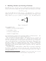
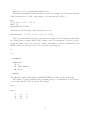
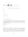
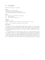
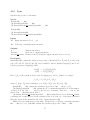
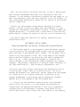
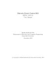
In the RW supervisory control theory [3], it is assumed that the plant and the design specifications can be modeled as finite–state automata. A finite–state automaton is a five–tuple
G = (X, Σ, η, x0 , Xm )
where X is the finite state set, Σ the event set, x0 the initial state, Xm ⊆ X the set of
marked states and η : X × Σ → X is the transition (partial) function. An example is given
in Fig. 1 with X = {1, 2, 3}, Σ = {11, 12}, x0 = 1 and Xm = {2, 3}. The marked states are
11
G
2
12
1
11
3
Figure 1: Automaton G.
shown with thick circles.
In DECK, an automaton is characterized by
1. N, the number of states,
2. TL, the list of transitions, and
3. Xm, the set of marked states.
N is a nonnegative (N ≥ 0) integer. For an automaton with N ≥ 1, the state set is {1, . . . , N},
with 1 used for the initial state. For an empty automaton, N = 0.
The event labels are nonnegative integers 1 . Zero (0) is reserved for clock tick. In
supervisory control, the event set is partitioned into controllable and uncontrollable event
sets. The controllability status of an event depends on the extent and scope of a supervisor’s
control over the plant and hence on both the plant and the supervisor. This issue becomes
important, for instance, in decentralized supervisory control. Therefore, in DECK when
an automaton is defined, the controllable/uncontrollable status of events are not specified.
This status is declared only when a function related to supervisory control (i.e., supcon and
controllable) is used.
TL (transition list) is a matrix with three columns. Each row represents a transition in
the form [x1 e x2], where x1, e and x2 are the source state, event and target state. The
event set Σ is implicitly taken to be the event labels that appear in the second column of
the transition list, TL.
1
The default type for numerical variables in MATLAB is double precision floating point. To prevent
roundoff errors in storing integer labels, the event labels should be no larger than 9 × 1015 .
3
Xm is a row vector containing the marked states.
The function automaton builds automaton objects. For example, the following statements
build an automaton object G corresponding to the automaton G in Fig. 1.
N=3;
TL=[1 11 2; 2 12 3; 3 11 1];
Xm=[2 3];
G=automaton(N,TL,Xm);
Alternatively, the following compact form may be used.
G=automaton(3, [1 11 2; 2 12 3; 3 11 1], [2 3]);
The vector Xm (marked states) is optional and if omitted in the automaton statement,
the default value of empty (Xm=[]) will be taken. Once the automaton object G is created,
typing G returns a list of its properties, namely, the number of states, transition list and
marked states (An automaton object does not have any methods).
G
G =
automaton
Properties:
N: 3
TL: [3x3 double]
Xm: [2 3]
Methods
Note that thoroughout this manual, MATLAB/DECK responses are shown in italics.
The number of states, transition list and marked states of an automaton object G can be
accessed through G.N, G.TL and G.Xm. For example:
G.TL
ans =
1
2
3
11
12
11
2
3
1
4
The function automatonchk can be used to verify that an automaton object conforms
to the conventions of DECK for naming states and event labels. This function is useful for
checking DECK models that are created for the first time or imported from an input file. It
can also help with debugging new functions developed in the DECK environment.
After the desired automata are built, they can be analyzed and manipulated using the
available functions in DECK. The reach function can be used to perform reachability analysis on the transition graphs of automata. The function reachable and trim return the
reachable and trim subautomata while complement finds the complement of an automaton.
The selfloop function adjoins selfloops to each state of its input automaton.
The functions product and sync perform the parallel product (also known as “meet”)
and the synchronous product of an arbitrary number of automata G1, ..., Gn. The product
and sync functions can also find the parallel and synchrnous products of an array of automata. Furthermore, for every state of the resulting automaton, these functions return the
information about the state of each of the constituent automata G1, ..., Gn.
Finally, the function supcon can be used to find the supremal controllable sublanguage
and design minimally restrictive supervisor. The function controllable can be used to see
if a language is controllable and in cases where controllability test fails, to obtain information
about the circumstances under which the property has failed.
More details about each function is provided in Sec. 4 (Toolbox Functions). In the
following section, two illustrative examples will be discussed.
5
3
3.1
Examples
Small Factory
This example has two parts. First it illustrates supervisor design using the Small Factory
problem (Example 3.4.4, [5]). Next, it explains how it can be verified whether the plant
(small factory) under the supervision of a given supervisor meets the design specifications.
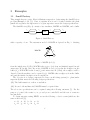
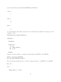
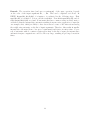
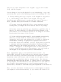
The Small Factory (Fig. 2) consists of two machines, MACH1 and MACH2, and a buffer
β1
α1
MACH1
α2
β2
BUF
MACH2
Figure 2: Small Factory.
with a capacity of one. The automaton model of MACHi is depicted in Fig. 3. Starting
1
αi
MACHi
βi
2
λi
µi
3
Figure 3: MACHi (i=1,2).
from the initial state I (idle), MACH1 takes a piece (α1 ) from an (infinite) input bin and
enters state W (work). Once the work of MACH1 is done, it deposits the workpiece in the
buffer (β1 ). If MACH1 breaks down (λ1 ) and enters state D (down), the workpiece will be
discarded but the machine can be repaired (µ1 ). MACH2 takes workpieces from the buffer
and puts the finished workpieces in an output bin.
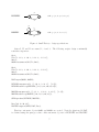
The objective is to design a supervisor to have a nonblocking system (i.e. plant under
supervision) that meets the following design specifications.
(S1) The buffer must not oveflow or underflow.
(S2) In case both machines fail, MACH2 must be repaired first.
The above two specifications can be captured using the following automata [5]. For the
purpose of control, the events α1 , α2 , µ1 and µ2 are controllable and the rest of events are
uncontrollable.
To design supervisor using DECK, we use the following codes for events (which are the
same as those in [5]).
α1 : 11 β1 : 10 λ1 : 12 µ1 : 13
α2 : 21 β2 : 20 λ2 : 22 µ2 : 23
6
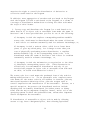
β1
BUFSPEC
1
2
selfloop {α1 , λ1 , µ1 , β2 , λ2 , µ2 }
2
selfloop {α1 , β1 , λ1 , α2 , β2 }
α2
µ1
λ2
BRSPEC
1
µ2
Figure 4: Small Factory: design specifications.
States I, W and D are named 1, 2 and 3. The following scripts design a minimally
restrictive supervisor.
N1=3;
TL1=[1 11 2; 2 10 1; 2 12 3; 3 13 1];
Xm1=1;
MACH1=automaton(N1,TL1,Xm1);
N2=3;
TL2=[1 21 2; 2 20 1; 2 22 3; 3 23 1];
Xm2=1;
MACH2=automaton(N2,TL2,Xm2);
FACT=sync(MACH1,MACH2);
BUFSPEC=automaton(2, [1 10 2; 2 21 1], [1 2]);
BUFSPEC=selfloop(BUFSPEC,[11,13,14,20,22,23]);
BRSPEC=automaton(2, [1 13 1; 1 22 2; 2 23 1], [1 2]);
BRSPEC=selfloop(BRSPEC,[10,11,13,20,21]);
SPEC=product(BUFSPEC,BRSPEC);
Euc=[10 12 20 22];
FACTSUP=supcon(SPEC,FACT,Euc);
First two automata objects MACH1 and MACH2 are created. Next the plant model FACT
is obtained using the sync procedure. After automata objects for BUFSPEC and BRSPEC
7
are built, the automaton object SPEC is found using the product command. Finally the
set of uncontrollable events are defined and the supervisor (in the form of an automaton
FACTSUP) is obtained using supcon. FACTSUP has 12 states and 24 transitions.
FACTSUP
FACTSUP =
automaton
Properties:
N: 12
TL: [24x3 double]
Xm: [1 3]
Methods
The transition list and marked states can be examined as follows.
FACTSUP.TL
ans =
1
2
2
3
4
5
5
5
6
6
6
6
7
7
8
8
8
9
9
10
10
11
10
12
21
13
11
20
22
10
12
20
22
11
23
13
20
22
20
22
10
12
2
3
4
5
1
6
1
7
9
8
2
10
10
1
5
4
11
3
12
12
11
8
β1
BUFSUP
1
2
selfloop {α1 , λ1 , µ1 , β2 , λ2 , µ2 }
α2
Figure 5: Small Factory: proposed supervisor BUFSUP.
10
11
12
23
23
23
2
4
3
FACTSUP.Xm
ans =
1
3
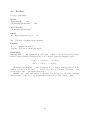
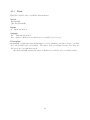
In the second part of this problem, let us consider Small Factory again with the objective
of finding a nonblcking supervisor enforcing design specification S1 (regarding buffer overflow
and underflow). First suppose the automaton in Fig. 5 has been proposed for supervisor.
Note that this automaton is the same as the spec automaton BUFSPEC. The following script
first builds the plant model which contains 9 states. This time, in addition to FACT, we have
decided to get the information of the states of the components (MACH1 and MACH2) in the 9×2
matrix FACT States. Next the proposed suprevisor BUFSUP is built and the controllable
procedure is used to determine if BUFSUP is admissible (i.e., the closed behavior L(BUFSUP)
is controllable).
MACH1=automaton(3, [1 11 2; 2 10 1; 2 12 3; 3 13 1], 1);
MACH2=automaton(3, [1 21 2; 2 20 1; 2 22 3; 3 23 1], 1);
[FACT,FACT States]=sync(MACH1,MACH2);
BUFSPEC=automaton(2, [1 10 2; 2 21 1], [1 2]);
BUFSPEC=selfloop(BUFSPEC,[11 12 13 20 22 23]);
BUFSUP=automaton(2, [1 10 2; 2 21 1],[1 2]);
BUFSUP=selfloop(BUFSUP,[11 12 13 20 22 23]);
Euc=[10 12 20 22];
[ic,S,E]=controllable(BUFSUP,FACT,Euc)
The results are returned in ic, S, E.
9
α1
β1
BUFSUPrev
1
2
selfloop {λ1 , µ1 , β2 , λ2 , µ2 }
α2
Figure 6: Small Factory: revised supervisor.
ic =
0
S =
2
2
2
2
5
8
E =
[10]
[10]
[10]
It is observed that BUFSUP is not admissible. Uncontrollable event disablement would
occur when the plant and supervisor are in states given by the rows of S. The corresponding
disabled uncontrollable events are provided in E. For instance, one such disablement occurs
when FACT and BUFSPEC are in states 2 and 2. To determine the states of MACH1 and MACH2
when FACT is in state 2, we use
FACT_States(2,:)
ans =
2
1
Thus MACH1 is in state 2 and MACH2 in state 1. In other words, when the buffer is full, MACH1
is in state 2 (W) and potentially ready to deposit another workpiece in the buffer, BUPSUP
attempts to disable the uncontrollable event β1 (event 10). In order to correct this issue, we
remove the α1 selfloop in state 2 of BUFSUP after the occurrence of β1 (workpiece deposit
in buffer) and effectively disable controllable event α1 when the buffer is full. The resulting
supervisor BUFSUPrev is shown in Fig. 6. We can see that this supervisor is addmissible.
10
[icrev,Srev,Erev]=controllable(BUFSUPrev,FACT,Euc)
icrev =
1
Srev =
[]
Erev =
{}
To verify that the plant under supervision is nonblocking and satisfies the design spec, first
it must be built.
FACTuSUP=product(FACT,BUFSUPrev)
FACTuSUP =
automaton
Properties:
N: 12
TL: [25x3 double]
Xm: [1 3]
Methods
Next the automaton FSco is constructed which marks Lm (FACT) ∩ [Lm (SPEC)]co .
SPECco=complement(BUFSPEC);
FSco=product(FACTuSUP,SPECco)
We note that the marked state set of FSco is empty and hence, Lm (FACT) ⊆ Lm (SPEC).
FSco.Xm
ans =
Empty matrix: 1-by-0
11
Pi
αi
1
γi
βi
βi
k+1
2
k+2
µi
Figure 7: Dining Philosophers: Philosopher Pi .
Finally, to see if the (reachable) automaton FACTuSUP is nonblocking, the trim procedure
is used.
FACTuSUPt=trim(FACTuSUP)
FACTuSUPt =
automaton
Properties:
N: 12
TL: [25x3 double]
Xm: [1 3]
Methods
FACTuSUP has the same number of states as FACTuSUPt and hence it is nonblocking.
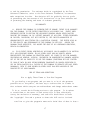
3.2
Dining Philosophers
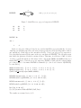
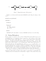
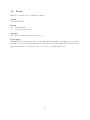
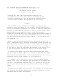
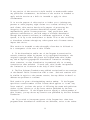
In this example, an extension of the problem of Dining Philosophers (which was proposed
in WODES 2008 as a benchmark problem for supervisory control software tools) is examined. In this problem, n philosophers P1 , . . . , Pn (n ≥ 2) are seated around a table and n
forks F1 , . . . , Fn placed on the table in the following order: F1 , P1 , F2 , P2 , . . . , Fn , Pn . The
automaton modeling philosopher Pi is shown in Fig. 7. Philosopher Pi takes the fork on his
left Fi (event αi ) and executes k − 1 (k ≥ 1) intermediate events βi till it reaches state k + 1.
Then it takes the fork on his right (that is Fi+1 when 1 ≤ i ≤ n − 1, and F1 when i = n.)
and enters eating state k + 2 (event γi ). Finally, Pi returns the forks (event µi ) and goes to
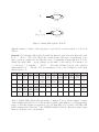
its initial (idle) state. The automata for forks are shown in Fig. 8. The events “philosopher
takes the left fork” (αi ) are assumed uncontrollable when i is even. The rest of events are
controllable. The objective is to design a maximally permissive nonblocking supervisor.
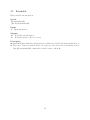
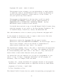
The script for solving the problem is provided at the end of this section. Note that the
automata for philosophers and forks are put together to form an array of automata Gs. The
commands tic and toc measure the execution time of supcon. The execution time, along
12
α1 , γn
F1
1
2
µ1 , µn
γi−1 , αi
Fi
1
(2 ≤ i ≤ n)
2
µi−1 , µi
Figure 8: Dining Philosophers: Fork Fi .
with the number of states of the supervisor, is provided for various values of n and k in
Table 1.
Remark: Note that the philosopher and fork automata are placed in array Gs in the order
F1 , P1 , . . . , Fn , Pn . The order affects the execution time (and space requirement) of the
sync operation (despite the fact that the order of arguments in sync function does not
change the final result – except perhaps for the name of the states). For instance, for
n = 10 and k = 1, sync(P1,...,Pn,F1,...,Fn) takes 24 times longer to run compared
with sync(F1,P1,...,Fn,Pn). For an explanation, refer to the description of the sync
function in Sec. 4.
k\n
1
2
4
8
16
2
<0.1
3
<0.1
4
<0.1
6
<0.1
10
<0.1
18
3
<0.1
12
<0.1
24
<0.1
60
0.3
180
2
612
4
<0.1
30
<0.1
83
0.4
327
4.8
1703
313
10695
5
<0.1
78
0.3
321
3.5
2175
325
21267
6
0.2
190
1.4
1082
69
11602
7
0.5
470
7.9
3855
2795
69785
8
1.7
1138
89.8
12863
9
5.8
2770
1240
44172
10
28.1
6694
11
185
16206
12
1476
39138
T (sec)
N
T (sec)
N
T (sec)
N
T (sec)
N
T (sec)
N
Table 1: Dining Philosophers: Execution time of supcon, T (sec), and the number of states
of the resulting automaton, N, for various values of philosopher number, n, and intermediate
states, k. Execution times are measured on a PC with Intel Core i5-2500, 3.10 GHz, 8GB
RAM, running 64-bit Windows 7 and MATLAB R2011b (64-bit). Execution times longer
than one hour have not been measured.
13
Script for solving the problem of Dining Philosophers
%
% Solves the "Dining Philosophers" benchmark problem of WODES 2008
%
%
display(’Dining Philosophers’)
% Number of philosophers (and forks) (n>=2)
n=9;
fprintf(’Number of philosophers (n): %d\n’, n)
% Number of intermediate states (k>=1)
k=1;
fprintf(’Number of intermediate states (k): %d\n’, k)
%
% Plant model (G)
%
display(’Building Plant model (G)’)
%
% Event coding
%
% For philosopher Pi:
%
alpha(i)=10*i+1
beta(i)=10*i+2
%
alpha=10*(1:n)+1;
beta=10*(1:n)+2;
gamma=10*(1:n)+3;
mu=10*(1:n)+4;
gamma(i)=10*i+3
%
% Gs is an array of the automata of Philosophers and Forks
% in the order F1, P1, F2, P2, ..., Fn, Pn.
for i=1:2*n
Gs{i}=automaton(0,[],[]);
end
%
% Philosophers
%
for i=1:n
14
mu(i)=10*i+4
TLi=[1 alpha(i) 2];
for j=2:k
TLi=[TLi; j beta(i) j+1];
end
TLi=[TLi; k+1 gamma(i) k+2; k+2 mu(i) 1];
Gs{2*i}=automaton(k+2, TLi, 1);
end
%
% Forks
%
% The first fork
Gs{1}=automaton(2, [1 alpha(1) 2; 1 gamma(n) 2; 2 mu(1) 1; 2 mu(n) 1], 1);
%
% The other forks
for i=2:n
Gs{2*i-1}=automaton(2, [1 gamma(i-1) 2; 1 alpha(i) 2; ...
2 mu(i-1) 1; 2 mu(i) 1], 1);
end
%
G=sync(Gs);
%
% Spec (H)
%
display(’Building Spec model (H)’)
% Event set
if k==1
E=[alpha gamma mu];
else
E=[alpha beta gamma mu];
end
H=selfloop(automaton(1,[],1),E);
% Uncontrollable events
Euc=alpha(2:2:n);
%
display(’Supcon’)
15
tic
K=supcon(H,G,Euc);
toc
%
%
% End of code
16
4
Toolbox Functions
17
4.1
Automaton
Create an automaton model (‘automaton’ object) for use by Discrete Event Control Kit
(DECK).
Syntax
G=automaton(N,TL)
G=automaton(N,TL,Xm)
Inputs
N
Number of states
TL Transition list
Xm Marked states (row vector)
Outputs
G Output automaton
Description
The class ‘automaton’ has the following properties:
N Number of states.
The states must be named using the following convention: the state set must be {1,
..., N}, with 1 used for the initial state.
TL Transition list.
TL is an m-by-3 matrix where m is the number of transitions. Each row of TL represents a transition in the form [x1, sigma, x2], with x1 and x2 being the source and
destination states, and sigma, the corresponding event.
Xm Marked states (row vector).
G=automaton(N,TL,Xm) returns an automaton model (object) G with state set {1, ..., N},
transition list TL and set of marked states Xm.
G=automaton(N,TL) returns an automaton G with Xm=[].
18
4.2
Automatonchk
Verify the validity of an automaton object.
Syntax
flag1=automatonchk(G)
[flag1,flag2]=automatonchk(G)
Inputs
G Input automaton
Outputs
flag1 Automaton validity flag (part 1)
flag2 Automaton validity flag (part 2)
Description
[flag1,flag2]=automatonchk(G) verifies the validity of the automaton object G and returns
the result in flag1. In cases where the automaton is not valid, the invalid property is
identified in flag2. The various cases are explained in the following table.
Description
G.N has wrong size (is not a scalar)
G.TL has wrong size
G.Xm has wrong size
flag1
-3
-3
-3
flag2
1
2
3
-2
-2
-2
1
2
3
G.N is not an integer
G.TL contains entry that is not an integer
G.Xm contains entry that is not an integer
-1
-1
-1
1
2
3
G.N is negative
G.TL has out–of–range entry
G.Xm has out–of–range entry
(The valid range for states is 1,...,G.N,
and for events, nonnegative integers.)
0
0
2
3
G.TL has repeated rows
G.Xm has repeated entries
1
0
Automaton is valid
Automatonchk examines the above list of cases from the top. Once a case is identified,
the function returns with the corresponding flags.
19
4.3
Complement
Complement of a deterministic automaton.
Syntax
Gco=complement(G)
Gco=complement(G,Ea)
Inputs
G
Input deterministic automaton
Ea List of events (vector)
Outputs
Gco Output deterministic automaton
Description
Let E denote the event set of the input automaton G.
Gco=complement(G) returns an automaton Gco with
Lm (Gco ) = E ∗ − Lm (G),
L(Gco ) = E ∗
where Lm () and L() denote marked behavior (marked language) and closed behavior (generated language), and E ∗ is the Kleene closure of E.
Gco=complement(G,Ea) returns an automaton Gco with
Lm (Gco ) = Ee∗ − Lm (G),
L(Gco ) = Ee∗
where Ee = E ∪ Ea . The event set of the input automaton, E, and Ea must be disjoint.
20
4.4
Controllable
Determine if a language is controllable.
Syntax
isctrb=controllable(K,G,Euc)
[isctrb,States]=controllable(K,G,Euc)
[isctrb,States,Events]=controllable(K,G,Euc)
Inputs
K
Automaton representing the test language
G
Plant Automaton
Euc Uncontrollable events (vector)
Outputs
isctrb Test result
States List of states where disablement of uncontrollable events occurs
Events List of disabled uncontrollable events (cell array)
Description
Let Lm () and L() denote marked behavior (marked language) and closed behavior (generated language). isctrb=controllable(K,G,Euc) returns isctrb=1 if and only if L(K) is
controllable with respect to L(G) and Euc . Otherwise, it returns isctrb=0. When K is
trim, controllable(K,G,Euc) returns 1 if and only if Lm (K) is controllable with respect
to L(G) and Euc .
[isctrb,States]=controllable(K,G,Euc) returns a two-column matrix States. Each
row of States, [xK,xG], is a state of product(K,G) where disablement of uncontrollable
events (if any) occurs, i.e., the test fails. If L(K) is controllable (isctrb=1), then States=[].
[isctrb,States,Events]=controllable(K,G,Euc) returns the list of disabled uncontrollable events (if any) in the cell array Events. The i-th cell of Events, Events{i}, is a row
vector containing the uncontrollable events disabled in [xKi,xGi] (the i-th row of States).
21
4.5
Product
Product of automata.
Syntax
G=product(G1,...,Gn)
[G,States]=product(G1,...,Gn)
G=product(Ga)
[G,States]=product(Ga)
Inputs
Gi Input automaton i (i=1, ..., n)
Ga
Cell array containing input automata
Outputs
G
Output automaton
States State set of output automaton
Description
G=product(G1,...,Gn) returns the product of G1, ..., Gn (n >= 2). If Lm () and L() denote
marked behavior (marked language) and closed behavior (generated language), then
Lm (G) = Lm(G1 ) ∩ . . . ∩ Lm (Gn )
L(G) = L(G1 ) ∩ . . . ∩ L(Gn ).
[G,States]=product(G1,...,Gn) returns an N × n matrix States where N is the
number of states of G. Let [xi1 ... xin] be the i-th row of States. Then xi1, ..., xin
are the states of G1, ..., Gn when G is in state i.
PRODUCT can be used with arrays of automata. Let Ga denote a cell array containing
automata Ga1, ..., Gan (n >= 2). product(Ga) returns the product of Ga1, ..., Gan.
22
4.6
Reach
Find the reachable states of transition graph.
Syntax
Xr=reach(TL,S)
Inputs
TL Transition list
S
Source states (vector)
Outputs
Xr States reachable from S (row vector)
Description
Xr=reach(TL,S) returns the states of the (automaton) transition graph that are reachable
from the set of source states S using the breadth–first–search algorithm. The reachable states
appear in Xr in the order they are discovered in the breadth–first search.
23
4.7
Reachable
Find reachable subautomaton.
Syntax
Gr=reachable(G)
[Gr,Xr]=reachable(G)
Inputs
G Input automaton
Outputs
Gr Reachable subautomaton
Xr Reachable states of G (row vector)
Description
Gr=reachable(G) returns the subautomaton of G that is reachable (from the initial state of
G). The states of Gr are renamed in the order they are discovered in a breadth–first search.
[Gr,Xr]=reachable(G) returns the reachable states of G in Xr.
24
4.8
Selfloop
Add selfloops to automaton.
Syntax
Gs=selfloop(G,Es)
Inputs
G
Input automaton
Es List of events (vector)
Outputs
Gs Output automaton
Description
Adds selfloop transitions [x, e, x] to the transition list of the input automaton G, for all
states x of G and all events e in the event list Es. The event set of G and Es must be disjoint.
25
4.9
Supcon
Supremal Controllable Sublanguage.
Syntax
K=supcon(H,G,Euc)
Inputs
H
Specification (deterministic) automaton
G
Plant (deterministic) automaton
Euc Uncontrollable events (vector)
Outputs
K Trim (deterministic) automaton marking supremal controllable sublangage
Description
Let Lm () and L() denote marked behavior (marked language) and closed behavior (generated
language). SUPCON calculates the supremal sublanguage of Lm (H) ∩ Lm (G) that is controllable with respect to L(G) and Euc . The result is returned in the trim automaton K which
marks the supremal controllable sublanguage. The calculations are based on the algorithm
introduced in
W.M. Wonham and P.J. Ramadge, “On the supremal controllable sublanguage
of a given language,” SIAM J. Control and Optimization, Vol. 25, No. 3, May
1987.
26
4.10
Sync
Synchronous product of automata.
Syntax
G=sync(G1,...,Gn)
[G,States]=sync(G1,...,Gn)
[G,States,Blocked events]=sync(G1,...,Gn)
G=sync(Ga)
[G,States]=sync(Ga)
[G,States,Blocked events]=sync(Ga)
Inputs
Gi Input automaton i (i=1, ..., n)
Ga
Cell array containing input automata
Outputs
G
States
Blocked events
Output automaton
State set of output automaton
Events blocked (absent) in output automaton (row vector)
Description
G=sync(G1,G2) returns the synchronous product of G1 and G2. Let E1 and E2 be the event
sets of G1 and G2 . If Lm () and L() denote marked behavior (marked language) and closed
behavior (generated language), then
Lm (G) = Lm (G1 )kLm (G2 )
L(G) = L(G1 )kL(G2 )
Here L1 kL2 is the synchronous product of languages L1 and L2 defined according to
L1 kL2 = P1−1(L1 ) ∩ P2−1(L2 )
where P1 (resp. P2 ) is the natural project of (E1 ∪ E2 )∗ onto E1∗ (resp. E2∗ ).
G=sync(G1,...,Gn) returns the synchronous product of G1, ..., Gn (n >= 2).
[G,States]=sync(G1,...,Gn) returns the N × n matrix States where N is the number
of states of G. Let [xi1 ... xin] be the i-th row of States. Then xi1, ..., xin are the
states of G1, ..., Gn when G is in state i.
[G,States,Blocked events]=sync(G1,...,Gn) returns the row vector Blocked events
containing the events that are in the transition list of at least one of the input automata
(Gi) and absent in the transition list of the output automaton (G).
SYNC can be used with arrays of automata. Let Ga denote a cell array containing automata
Ga1, ..., Gan (n >= 2). sync(Ga) returns the synchronous product of Ga1, ..., Gan.
27
Remark: The execution time (and space requirement) of the sync operation depends
on the order of the input arguments G1, ..., Gn. This can be explained as follows. In
DECK, G=sync(G1,G2,G3,G4), for instance, is evaluated in the following steps. First
sync(G1,G2) is calculated. Let us call the result G12. Next G123=sync(G12,G3) and finally G=sync(G123,G4) are found. If automata that have common events are listed next to
eachother, then the intermediate automata resulting from successive application of sync (in
our example, G12, G123) are likely to have fewer states because of the interactions among
the neighboring automata on the list of input arguments. Therefore, this results in smaller
intermediate automata (hence, less space requirement) and faster execution time. Coversely, if automata with no common events appear first on the list of sync, the intermediate
automata in sync computations could become very large, resulting in prolonged execution
times.
28
4.11
Trim
Find the reachable and coreachable subautomaton.
Syntax
Gt=trim(G)
[Gt,Xrc]=trim(G)
Inputs
G Input automaton
Outputs
Gt
Trim subautomaton
Xrc States of G that are reachable and coreachable (row vector)
Description
Gt=trim(G) returns the trim subautomaton of G (containing only those states of G that
are both reachable and coreachable). The states of Gt are renamed in the order they are
discovered in a breadth–first search.
[Gt,Xrc]=trim(G) returns the states of G that are reachable and coreachable in Xrc.
29
A
Installation
Simply unzip the downloaded file. If you wish to keep your data files and scripts in a separate
directory (folder) and run DECK from that directory, then from MATLAB menu bar, use
“File” followed by “Set path” to add the directory of DECK files to MATLAB’s search path.
Alternatively, this can be done using the command “path”.
30
B
GNU General Public License, v.2
GNU GENERAL PUBLIC LICENSE
Version 2, June 1991
Copyright (C) 1989, 1991 Free Software Foundation, Inc.,
51 Franklin Street, Fifth Floor, Boston, MA 02110-1301 USA
Everyone is permitted to copy and distribute verbatim copies
of this license document, but changing it is not allowed.
Preamble
The licenses for most software are designed to take away your
freedom to share and change it. By contrast, the GNU General Public
License is intended to guarantee your freedom to share and change free
software--to make sure the software is free for all its users. This
General Public License applies to most of the Free Software
Foundation’s software and to any other program whose authors commit to
using it. (Some other Free Software Foundation software is covered by
the GNU Lesser General Public License instead.) You can apply it to
your programs, too.
When we speak of free software, we are referring to freedom, not
price. Our General Public Licenses are designed to make sure that you
have the freedom to distribute copies of free software (and charge for
this service if you wish), that you receive source code or can get it
if you want it, that you can change the software or use pieces of it
in new free programs; and that you know you can do these things.
To protect your rights, we need to make restrictions that forbid
anyone to deny you these rights or to ask you to surrender the rights.
These restrictions translate to certain responsibilities for you if you
distribute copies of the software, or if you modify it.
For example, if you distribute copies of such a program, whether
gratis or for a fee, you must give the recipients all the rights that
you have. You must make sure that they, too, receive or can get the
source code. And you must show them these terms so they know their
rights.
We protect your rights with two steps: (1) copyright the software, and
(2) offer you this license which gives you legal permission to copy,
distribute and/or modify the software.
31
Also, for each author’s protection and ours, we want to make certain
that everyone understands that there is no warranty for this free
software. If the software is modified by someone else and passed on, we
want its recipients to know that what they have is not the original, so
that any problems introduced by others will not reflect on the original
authors’ reputations.
Finally, any free program is threatened constantly by software
patents. We wish to avoid the danger that redistributors of a free
program will individually obtain patent licenses, in effect making the
program proprietary. To prevent this, we have made it clear that any
patent must be licensed for everyone’s free use or not licensed at all.
The precise terms and conditions for copying, distribution and
modification follow.
GNU GENERAL PUBLIC LICENSE
TERMS AND CONDITIONS FOR COPYING, DISTRIBUTION AND MODIFICATION
0. This License applies to any program or other work which contains
a notice placed by the copyright holder saying it may be distributed
under the terms of this General Public License. The "Program", below,
refers to any such program or work, and a "work based on the Program"
means either the Program or any derivative work under copyright law:
that is to say, a work containing the Program or a portion of it,
either verbatim or with modifications and/or translated into another
language. (Hereinafter, translation is included without limitation in
the term "modification".) Each licensee is addressed as "you".
Activities other than copying, distribution and modification are not
covered by this License; they are outside its scope. The act of
running the Program is not restricted, and the output from the Program
is covered only if its contents constitute a work based on the
Program (independent of having been made by running the Program).
Whether that is true depends on what the Program does.
1. You may copy and distribute verbatim copies of the Program’s
source code as you receive it, in any medium, provided that you
conspicuously and appropriately publish on each copy an appropriate
copyright notice and disclaimer of warranty; keep intact all the
notices that refer to this License and to the absence of any warranty;
32
and give any other recipients of the Program a copy of this License
along with the Program.
You may charge a fee for the physical act of transferring a copy, and
you may at your option offer warranty protection in exchange for a fee.
2. You may modify your copy or copies of the Program or any portion
of it, thus forming a work based on the Program, and copy and
distribute such modifications or work under the terms of Section 1
above, provided that you also meet all of these conditions:
a) You must cause the modified files to carry prominent notices
stating that you changed the files and the date of any change.
b) You must cause any work that
whole or in part contains or is
part thereof, to be licensed as
parties under the terms of this
you distribute or publish, that in
derived from the Program or any
a whole at no charge to all third
License.
c) If the modified program normally reads commands interactively
when run, you must cause it, when started running for such
interactive use in the most ordinary way, to print or display an
announcement including an appropriate copyright notice and a
notice that there is no warranty (or else, saying that you provide
a warranty) and that users may redistribute the program under
these conditions, and telling the user how to view a copy of this
License. (Exception: if the Program itself is interactive but
does not normally print such an announcement, your work based on
the Program is not required to print an announcement.)
These requirements apply to the modified work as a whole. If
identifiable sections of that work are not derived from the Program,
and can be reasonably considered independent and separate works in
themselves, then this License, and its terms, do not apply to those
sections when you distribute them as separate works. But when you
distribute the same sections as part of a whole which is a work based
on the Program, the distribution of the whole must be on the terms of
this License, whose permissions for other licensees extend to the
entire whole, and thus to each and every part regardless of who wrote it.
Thus, it is not the intent of this section to claim rights or contest
your rights to work written entirely by you; rather, the intent is to
33
exercise the right to control the distribution of derivative or
collective works based on the Program.
In addition, mere aggregation of another work not based on the Program
with the Program (or with a work based on the Program) on a volume of
a storage or distribution medium does not bring the other work under
the scope of this License.
3. You may copy and distribute the Program (or a work based on it,
under Section 2) in object code or executable form under the terms of
Sections 1 and 2 above provided that you also do one of the following:
a) Accompany it with the complete corresponding machine-readable
source code, which must be distributed under the terms of Sections
1 and 2 above on a medium customarily used for software interchange; or,
b) Accompany it with a written offer, valid for at least three
years, to give any third party, for a charge no more than your
cost of physically performing source distribution, a complete
machine-readable copy of the corresponding source code, to be
distributed under the terms of Sections 1 and 2 above on a medium
customarily used for software interchange; or,
c) Accompany it with the information you received as to the offer
to distribute corresponding source code. (This alternative is
allowed only for noncommercial distribution and only if you
received the program in object code or executable form with such
an offer, in accord with Subsection b above.)
The source code for a work means the preferred form of the work for
making modifications to it. For an executable work, complete source
code means all the source code for all modules it contains, plus any
associated interface definition files, plus the scripts used to
control compilation and installation of the executable. However, as a
special exception, the source code distributed need not include
anything that is normally distributed (in either source or binary
form) with the major components (compiler, kernel, and so on) of the
operating system on which the executable runs, unless that component
itself accompanies the executable.
If distribution of executable or object code is made by offering
access to copy from a designated place, then offering equivalent
34
access to copy the source code from the same place counts as
distribution of the source code, even though third parties are not
compelled to copy the source along with the object code.
4. You may not copy, modify, sublicense, or distribute the Program
except as expressly provided under this License. Any attempt
otherwise to copy, modify, sublicense or distribute the Program is
void, and will automatically terminate your rights under this License.
However, parties who have received copies, or rights, from you under
this License will not have their licenses terminated so long as such
parties remain in full compliance.
5. You are not required to accept this License, since you have not
signed it. However, nothing else grants you permission to modify or
distribute the Program or its derivative works. These actions are
prohibited by law if you do not accept this License. Therefore, by
modifying or distributing the Program (or any work based on the
Program), you indicate your acceptance of this License to do so, and
all its terms and conditions for copying, distributing or modifying
the Program or works based on it.
6. Each time you redistribute the Program (or any work based on the
Program), the recipient automatically receives a license from the
original licensor to copy, distribute or modify the Program subject to
these terms and conditions. You may not impose any further
restrictions on the recipients’ exercise of the rights granted herein.
You are not responsible for enforcing compliance by third parties to
this License.
7. If, as a consequence of a court judgment or allegation of patent
infringement or for any other reason (not limited to patent issues),
conditions are imposed on you (whether by court order, agreement or
otherwise) that contradict the conditions of this License, they do not
excuse you from the conditions of this License. If you cannot
distribute so as to satisfy simultaneously your obligations under this
License and any other pertinent obligations, then as a consequence you
may not distribute the Program at all. For example, if a patent
license would not permit royalty-free redistribution of the Program by
all those who receive copies directly or indirectly through you, then
the only way you could satisfy both it and this License would be to
refrain entirely from distribution of the Program.
35
If any portion of this section is held invalid or unenforceable under
any particular circumstance, the balance of the section is intended to
apply and the section as a whole is intended to apply in other
circumstances.
It is not the purpose of this section to induce you to infringe any
patents or other property right claims or to contest validity of any
such claims; this section has the sole purpose of protecting the
integrity of the free software distribution system, which is
implemented by public license practices. Many people have made
generous contributions to the wide range of software distributed
through that system in reliance on consistent application of that
system; it is up to the author/donor to decide if he or she is willing
to distribute software through any other system and a licensee cannot
impose that choice.
This section is intended to make thoroughly clear what is believed to
be a consequence of the rest of this License.
8. If the distribution and/or use of the Program is restricted in
certain countries either by patents or by copyrighted interfaces, the
original copyright holder who places the Program under this License
may add an explicit geographical distribution limitation excluding
those countries, so that distribution is permitted only in or among
countries not thus excluded. In such case, this License incorporates
the limitation as if written in the body of this License.
9. The Free Software Foundation may publish revised and/or new versions
of the General Public License from time to time. Such new versions will
be similar in spirit to the present version, but may differ in detail to
address new problems or concerns.
Each version is given a distinguishing version number. If the Program
specifies a version number of this License which applies to it and "any
later version", you have the option of following the terms and conditions
either of that version or of any later version published by the Free
Software Foundation. If the Program does not specify a version number of
this License, you may choose any version ever published by the Free Software
Foundation.
10. If you wish to incorporate parts of the Program into other free
programs whose distribution conditions are different, write to the author
36
to ask for permission. For software which is copyrighted by the Free
Software Foundation, write to the Free Software Foundation; we sometimes
make exceptions for this. Our decision will be guided by the two goals
of preserving the free status of all derivatives of our free software and
of promoting the sharing and reuse of software generally.
NO WARRANTY
11. BECAUSE THE PROGRAM IS LICENSED FREE OF CHARGE, THERE IS NO WARRANTY
FOR THE PROGRAM, TO THE EXTENT PERMITTED BY APPLICABLE LAW. EXCEPT WHEN
OTHERWISE STATED IN WRITING THE COPYRIGHT HOLDERS AND/OR OTHER PARTIES
PROVIDE THE PROGRAM "AS IS" WITHOUT WARRANTY OF ANY KIND, EITHER EXPRESSED
OR IMPLIED, INCLUDING, BUT NOT LIMITED TO, THE IMPLIED WARRANTIES OF
MERCHANTABILITY AND FITNESS FOR A PARTICULAR PURPOSE. THE ENTIRE RISK AS
TO THE QUALITY AND PERFORMANCE OF THE PROGRAM IS WITH YOU. SHOULD THE
PROGRAM PROVE DEFECTIVE, YOU ASSUME THE COST OF ALL NECESSARY SERVICING,
REPAIR OR CORRECTION.
12. IN NO EVENT UNLESS REQUIRED BY APPLICABLE LAW OR AGREED TO IN WRITING
WILL ANY COPYRIGHT HOLDER, OR ANY OTHER PARTY WHO MAY MODIFY AND/OR
REDISTRIBUTE THE PROGRAM AS PERMITTED ABOVE, BE LIABLE TO YOU FOR DAMAGES,
INCLUDING ANY GENERAL, SPECIAL, INCIDENTAL OR CONSEQUENTIAL DAMAGES ARISING
OUT OF THE USE OR INABILITY TO USE THE PROGRAM (INCLUDING BUT NOT LIMITED
TO LOSS OF DATA OR DATA BEING RENDERED INACCURATE OR LOSSES SUSTAINED BY
YOU OR THIRD PARTIES OR A FAILURE OF THE PROGRAM TO OPERATE WITH ANY OTHER
PROGRAMS), EVEN IF SUCH HOLDER OR OTHER PARTY HAS BEEN ADVISED OF THE
POSSIBILITY OF SUCH DAMAGES.
END OF TERMS AND CONDITIONS
How to Apply These Terms to Your New Programs
If you develop a new program, and you want it to be of the greatest
possible use to the public, the best way to achieve this is to make it
free software which everyone can redistribute and change under these terms.
To do so, attach the following notices to the
to attach them to the start of each source file
convey the exclusion of warranty; and each file
the "copyright" line and a pointer to where the
program. It is safest
to most effectively
should have at least
full notice is found.
<one line to give the program’s name and a brief idea of what it does.>
37
Copyright (C) <year>
<name of author>
This program is free software; you can redistribute it and/or modify
it under the terms of the GNU General Public License as published by
the Free Software Foundation; either version 2 of the License, or
(at your option) any later version.
This program is distributed in the hope that it will be useful,
but WITHOUT ANY WARRANTY; without even the implied warranty of
MERCHANTABILITY or FITNESS FOR A PARTICULAR PURPOSE. See the
GNU General Public License for more details.
You should have received a copy of the GNU General Public License along
with this program; if not, write to the Free Software Foundation, Inc.,
51 Franklin Street, Fifth Floor, Boston, MA 02110-1301 USA.
Also add information on how to contact you by electronic and paper mail.
If the program is interactive, make it output a short notice like this
when it starts in an interactive mode:
Gnomovision version 69, Copyright (C) year name of author
Gnomovision comes with ABSOLUTELY NO WARRANTY; for details type ‘show w’.
This is free software, and you are welcome to redistribute it
under certain conditions; type ‘show c’ for details.
The hypothetical commands ‘show w’ and ‘show c’ should show the appropriate
parts of the General Public License. Of course, the commands you use may
be called something other than ‘show w’ and ‘show c’; they could even be
mouse-clicks or menu items--whatever suits your program.
You should also get your employer (if you work as a programmer) or your
school, if any, to sign a "copyright disclaimer" for the program, if
necessary. Here is a sample; alter the names:
Yoyodyne, Inc., hereby disclaims all copyright interest in the program
‘Gnomovision’ (which makes passes at compilers) written by James Hacker.
<signature of Ty Coon>, 1 April 1989
Ty Coon, President of Vice
This General Public License does not permit incorporating your program into
38
proprietary programs. If your program is a subroutine library, you may
consider it more useful to permit linking proprietary applications with the
library. If this is what you want to do, use the GNU Lesser General
Public License instead of this License.
39
References
[1] C.G. Cassandras and S. Lafortune, Introduction to Discrete Event Systems, Springer,
2008.
[2] Mathworks Inc., MATLAB, http://www.mathworks.com/help/matlab/index.html.
[3] P.J. Ramadge and W.M. Wonham, “Supervisory control of a class of discrete event
processes,” SIAM J. Control Optim., vol. 25, no. 1, pp. 206-230, 1987.
[4] W.M. Wonham and P.J. Ramadge,“On the supremal controllable sublanguage of a given
language,” SIAM J. Control Optim., vol. 25, no. 3, pp. 635-659, 1987.
[5] W.M. Wonham, Supervisory Control of Discrete–Event Systems, Systems Control Group,
Edward S. Rogers Sr. Dept. of Electrical and Computer Engineering, University of
Toronto, Canada, 2012; available at http://www.control.utoronto.ca/DES.
40