Download Robert Fuster The xpicture package (http://www.upv.es/~rfuster

Robert Fuster
The xpicture package
(http://www.upv.es/~rfuster/xpicture)
Several extensions of the picture standard environment
User Manual
t
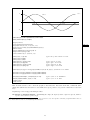
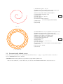
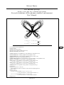
x = sin t ecos t − 2 cos 4t + sin5
12
t
y = cos t ecos t − 2 cos 4t + sin5
12
\setlength{\unitlength}{1cm}
\footnotesize
\DIVIDE{1}{12}{\invXII}
\MULTIPLY{12}{\numberTWOPI}{\phione}
\MULTIPLY{12}{64}{\divisions}
Ex. 1
\COMPOSITIONfunction{\EXPfunction}{\COSfunction}{\Afunction}
\SCALEVARIABLEfunction{4}{\COSfunction}{\Bfunction}
\SCALEVARIABLEfunction{\invXII}{\SINfunction}{\cfunction}
\POWERfunction{\cfunction}{5}{\Cfunction}
\LINEARCOMBINATIONfunction{1}{\Afunction}{-2}{\Bfunction}{\ABfunction}
\SUMfunction{\ABfunction}{\Cfunction}{\ABCfunction}
\PRODUCTfunction{\SINfunction}{\ABCfunction}{\Xfunction}
% x=(sin t)(exp(cos t)-2 cos 4t + (sin(t/12))^5)
\PRODUCTfunction{\COSfunction}{\ABCfunction}{\Yfunction}
% y=(cos t)(exp(cos t)-2 cos 4t + (sin(t/12))^5)
\PARAMETRICfunction{\Xfunction}{\Yfunction}{\butterfly}
\centering
\begin{Picture}(-4,-3)(4,4)
\PlotParametricFunction[\divisions]\butterfly{0}{\phione}
\end{Picture}
\begin{gather*}
x=\sin t\left(\mathrm e^{\cos t}-2\cos 4t
+\sin^5\left(\frac t{12}\right)\right) \\
y=\cos t\left(\mathrm e^{\cos t}-2\cos 4t
+\sin^5\left(\frac t{12}\right)\right)
\end{gather*}
2012/12/17
Contents
1 Introduction. New graphical instructions
3
2 A preliminary observation. Compatibility with text composition in color
3
3 Coordinate systems and the Picture environment
3.1 Coordinates . . . . . . . . . . . . . . . . . . . . . . . . . . .
3.1.1 Reference systems . . . . . . . . . . . . . . . . . . .
3.1.2 Polar coordinates . . . . . . . . . . . . . . . . . . . .
3.2 The Picture (or xpicture) environment . . . . . . . . . .
3.3 Coordinate axes . . . . . . . . . . . . . . . . . . . . . . . . .
3.3.1 The style of the axes . . . . . . . . . . . . . . . . . .
3.3.2 Axes position . . . . . . . . . . . . . . . . . . . . . .
3.3.3 Tags style . . . . . . . . . . . . . . . . . . . . . . . .
3.3.4 Tags position . . . . . . . . . . . . . . . . . . . . . .
3.3.5 Style of cut marks . . . . . . . . . . . . . . . . . . .
3.3.6 Removing and directly printing cut marks and labels
3.4 Cartesian grids . . . . . . . . . . . . . . . . . . . . . . . . .
3.4.1 Grid style . . . . . . . . . . . . . . . . . . . . . . . .
3.5 Polar grids . . . . . . . . . . . . . . . . . . . . . . . . . . .
.
.
.
.
.
.
.
.
.
.
.
.
.
.
.
.
.
.
.
.
.
.
.
.
.
.
.
.
.
.
.
.
.
.
.
.
.
.
.
.
.
.
.
.
.
.
.
.
.
.
.
.
.
.
.
.
.
.
.
.
.
.
.
.
.
.
.
.
.
.
.
.
.
.
.
.
.
.
.
.
.
.
.
.
.
.
.
.
.
.
.
.
.
.
.
.
.
.
.
.
.
.
.
.
.
.
.
.
.
.
.
.
.
.
.
.
.
.
.
.
.
.
.
.
.
.
.
.
.
.
.
.
.
.
.
.
.
.
.
.
.
.
.
.
.
.
.
.
.
.
.
.
.
.
.
.
.
.
.
.
.
.
.
.
.
.
.
.
.
.
.
.
.
.
.
.
.
.
.
.
.
.
.
.
.
.
.
.
.
.
.
.
.
.
.
.
.
.
.
.
.
.
.
.
.
.
.
.
.
.
.
.
.
.
.
.
.
.
.
.
.
.
.
.
.
.
.
.
.
.
.
.
.
.
.
.
.
.
.
.
.
.
.
.
.
.
.
.
.
.
.
.
.
.
.
.
.
.
.
.
.
.
.
.
.
.
.
.
.
.
.
.
.
.
.
.
.
.
.
.
.
.
.
.
.
.
.
.
.
.
.
.
.
.
3
3
4
5
6
7
8
9
9
9
10
10
12
13
13
4 Alternatives to some standard commands
4.1 Extensions of the \put command . . . . . .
4.1.1 Accurate positioning of the graphical
4.2 Alternatives to the \multiput command . .
4.3 Alternatives to \line and \vector . . . . .
4.4 Polygons anf polygonal lines . . . . . . . . .
. . . .
object
. . . .
. . . .
. . . .
.
.
.
.
.
.
.
.
.
.
.
.
.
.
.
.
.
.
.
.
.
.
.
.
.
.
.
.
.
.
.
.
.
.
.
.
.
.
.
.
.
.
.
.
.
.
.
.
.
.
.
.
.
.
.
.
.
.
.
.
.
.
.
.
.
.
.
.
.
.
.
.
.
.
.
.
.
.
.
.
.
.
.
.
.
.
.
.
.
.
.
.
.
.
.
.
.
.
.
.
.
.
.
.
.
.
.
.
.
.
.
.
.
.
.
.
.
.
.
.
.
.
.
.
.
.
.
.
.
.
15
15
16
23
24
25
5 Drawing curves
5.1 Conic sections . . . . . . . . . . . . . .
5.1.1 Circles . . . . . . . . . . . . . .
5.1.2 Ellipses . . . . . . . . . . . . .
5.1.3 Hyperbolas . . . . . . . . . . .
5.1.4 Parabolas . . . . . . . . . . . .
5.2 Arcs (of conic sections) . . . . . . . . .
5.3 Real variable functions . . . . . . . . .
5.3.1 Polynomial functions . . . . . .
5.3.2 Possible errors . . . . . . . . .
5.3.3 Accurate graphs . . . . . . . .
5.4 Polar coordinates curves . . . . . . . .
5.5 Parametrically defined curves . . . . .
5.5.1 The curve of the front page . .
5.6 Drawing curves from a table of values
.
.
.
.
.
.
.
.
.
.
.
.
.
.
.
.
.
.
.
.
.
.
.
.
.
.
.
.
.
.
.
.
.
.
.
.
.
.
.
.
.
.
.
.
.
.
.
.
.
.
.
.
.
.
.
.
.
.
.
.
.
.
.
.
.
.
.
.
.
.
.
.
.
.
.
.
.
.
.
.
.
.
.
.
.
.
.
.
.
.
.
.
.
.
.
.
.
.
.
.
.
.
.
.
.
.
.
.
.
.
.
.
.
.
.
.
.
.
.
.
.
.
.
.
.
.
.
.
.
.
.
.
.
.
.
.
.
.
.
.
.
.
.
.
.
.
.
.
.
.
.
.
.
.
.
.
.
.
.
.
.
.
.
.
.
.
.
.
.
.
.
.
.
.
.
.
.
.
.
.
.
.
.
.
.
.
.
.
.
.
.
.
.
.
.
.
.
.
.
.
.
.
.
.
.
.
.
.
.
.
.
.
.
.
.
.
.
.
.
.
.
.
.
.
.
.
.
.
.
.
.
.
.
.
.
.
.
.
.
.
.
.
.
.
.
.
.
.
.
.
.
.
.
.
.
.
.
.
.
.
.
.
.
.
.
.
.
.
.
.
.
.
.
.
.
.
.
.
.
.
.
.
.
.
.
.
.
.
.
.
.
.
.
.
.
.
.
.
.
.
.
.
.
.
.
.
.
.
.
.
.
.
.
.
.
.
.
.
.
.
.
.
.
.
.
.
.
.
.
.
.
.
.
.
.
.
.
.
.
.
.
.
.
.
.
.
.
.
.
.
.
.
.
.
.
.
.
.
.
.
.
.
.
.
.
.
.
.
.
.
.
.
.
.
.
.
.
.
26
26
26
27
27
28
31
33
43
43
44
46
48
51
52
.
.
.
.
.
.
.
.
.
.
.
.
.
.
.
.
.
.
.
.
.
.
.
.
.
.
.
.
.
.
.
.
.
.
.
.
.
.
.
.
.
.
.
.
.
.
.
.
.
.
.
.
.
.
.
.
.
.
.
.
.
.
.
.
.
.
.
.
.
.
.
.
.
.
.
.
.
.
.
.
.
.
.
.
6 Package options and configuration file
54
7 Compatibility with related packages
55
2
The xpicture package extends the picture standard environment and packages pict2e and curve2e,
adding the ability to work with arbitrary reference systems and with Cartesian or polar coordinates. In addition
to other utilities, the greater interest of xpicture lies in its capacity to draw function graphs, conic sections
and arcs, and parametrically defined curves.
This is the user manual of xpicture. Technical documentation and reference manual are contained in file
xpicture.pdf, distributed together with the package.
1
Introduction. New graphical instructions
The xpicture package introduces several new graphical instructions, and some enriched versions of standard
instructions used inside the picture environment. All these new instructions can be classified as follows:
• Reference systems and coordinates:
– Declaration and use of different reference systems, with Cartesian or polar coordinates.
– Instructions to show Cartesian or polar reference systems.
• An alternative to the picture environment, compatible with the new reference systems.
• Alternative instructions or extensions of the standard picture commands and those defined by the packages pict2e and curve2e:
– Enriched versions of marks \put and \multiput, providing an adequate control of the precise position
in which objects are composed (this functionality is especially useful in the composition of not strictly
graphical objects, such as formulas or labels).
– Instructions for drawing straight segments, vectors (in any direction and using any reference system),
polygonal lines, and regular and arbitrary polygons.
• Regular curves:
– Instructions for drawing conic sections (circles, ellipses, hyperbolas and parabolas) and arcs of these
curves.
– Instructions to graph functions and parametrically defined curves (this is the most interesting feature
of this package).
The only requeriments for xpicture are packages calculator, calculus, curve2e and xcolor. Therefore, it
works with any TEX extension compatible with these packages. You can compile a document including xpicture
pictures directly with pdflatex, lualatex, xelatex or indirectly, via latex/dvips, latex/dvips/dvipdfm,
. . . Pure dvi files are not supported, but some dvi previewers may show partially xpicture draws included in
dvi files.
2
A preliminary observation. Compatibility with text composition in
color
The xpicture package automatically loads the xcolor package. So, we can compose our pictures (and the
whole document) in various colors. However, when used in the body of the picture environment, marks \color
and \colortext often introduce spurious spaces. For this reason, the xpicture package introduces the new
command \pictcolor.
\pictcolor{color }
This mark behaves like the \color command, but does not produces these inappropriate spaces. To change
colors inside a picture, instead of \color or \colortext, use always the \pictcolor declaration.
3
3.1
Coordinate systems and the Picture environment
Coordinates
The standard picture environment establishes a rectangular coordinate system, so that all graphic objects are
placed in the picture using the canonical coordinates of the plane. From now on, we will call this reference
system the standard reference system. Loading the xpicture package, we can use any other affine reference
system and combine it with the use of polar coordinates.
3
3.1.1
Reference systems
The xpicture package allows us to use other reference systems. For the purpose we are interested, a reference
system consists of an origin of coordinates and a pair of linearly independent vectors. Typing
\referencesystem(x0 ,y0 )(x1 ,y1 )(x2 ,y2 )
we declare the new reference system with origin at point (x0 , y0 ) and coordinate vectors (x1 , y1 ) and (x2 , y2 ).
If the coordinates of the point P with respect to this reference system are (x̄ , ȳ ), then the coordinates of P
with respect to the standard system, (x , y ), are calculated with the formula
x
x0
x1 x2 x̄
=
+
y
y0
y1 y2 ȳ
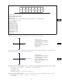
For example,
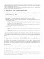
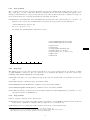
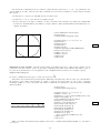
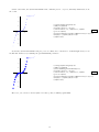
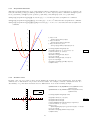
\referencesystem(1,2)(1,0)(0.5,0.5)
sets a new reference system that has its origin in the point O(1, 2) and the coordinate vectors ~u1 = (1, 0) and
~u2 = (1/2, 1/2). The following pictures show this coordinate system built on the standard reference system and
a Cartesian grid refered to the new reference system.
2
1
−2
O
−1
~u2
u1 2
1 ~
−1
−2
3
2
1
−3
−2
−1
1
2
3
−1
−2
−3
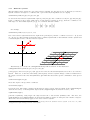
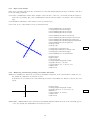
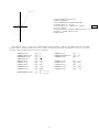
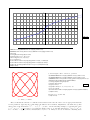
Alternatively, you can use the \changereferencesystem declaration: in the instruction
\changereferencesystem(x0 ,y0 )(x1 ,y1 )(x2 ,y2 )
point (x0 , y0 ) and vectors (x1 , y1 ) i (x2 , y2 ) are not refered to the standard system, but to the active reference
system.1 Moreover, as the more interesting (and frequent) reference system changes consist of translations of
the origin, rotations of the axes and symmetries, xpicture introduces three specific commands to these special
cases:
\translateorigin(x0 ,y0 )
moves the origin to the specified coordinates.
\rotateaxes{angle }
rotates the axes. The angle parameter is interpreted as the rotation angle in radians (if the \radiansangles
declaration is active) or in sexagesimal degrees (if the \degreesangles declaration is active). And
\symmetrize{angle }
performs a symmetry, being angle the angle between the x axis and the symmetry axis. Also here, the
\radiansangles and \degreesangles declarations determine if angles are interpreted as radians or degrees.
These three declarations always apply to the active reference system.
1 In other words, the instruction \referencesystem changes from the standard reference system to the new one, while
\changereferencesystem changes from the active system.
4
1
−1
1
2
3
4
5
6
7
8
9
10
11
12
13
14
−1
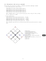
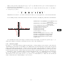
\newcommand{\mypicture}{%
{\thicklines
\xVECTOR(-1,-1)(1,1)
\pictcolor{red}\Circle{1}
\pictcolor{blue}\regularPolygon{1}{4}
\polarreference\degreesangles
\pictcolor{green}\Polygon(1,90)(0,0)(1,-30)}}
\centering
\setlength{\unitlength}{1cm}
\fbox{\begin{Picture}[black!5!white](-1.5,-6.5)(14.5,1.5)
\cartesiangrid(-1,-1)(14,1)
\mypicture
{\referencesystem(3,0)(1,1)(1,0)
\mypicture
\changereferencesystem(0,4)(-1,1)(1,-2)
\mypicture}
\degreesangles
\translateorigin(10,0)
{\rotateaxes{45}
\mypicture}
\translateorigin(3,0)
\symmetrize{45}
\mypicture
\referencesystem(6.5,-4)(7,0)(0,-2)\mypicture
\end{Picture}}
The \standardreferencesystem declaration restores the standard reference.
Changes of reference system can be used inside or outside the Picture environment. In the next sections
we will see what are the effects produced in each case.
3.1.2
Polar coordinates
Instead of Cartesian coordinates, we can refer to a point P using the polar coordinates (r, φ) of this point: r is
the distance from the origin O and φ is the angle between the first coordinate vector and the OP segment. The
\cartesianreference and \polarreference declarations establish the coordinates of one or the other type.
By default, the Cartesian coordinates are used, but in some cases is much easier determine polar coordinates.
Additionally, the \radiansangles and \degreesangles declarations sets angle measuring in radians or in
degrees, respectively (by default, angles are measured in radians).
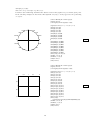
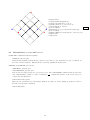
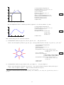
The following example shows a typical situation in which it is more appropriate to use polar coordinates:
the natural way to enter coordinates on a circle is using polar coordinates.
5
Ex. 2
\setlength{\unitlength}{3cm}
\fbox{\begin{Picture}(-1.3,-1.3)(1.3,1.3)
\polarreference
\degreesangles
xii
\renewcommand{\Pictlabelsep}{0.1}
\multiPut(1,0)(0,30){12}{\circle*{0.05}}
% Put twelve dots, one unit apart,
% at 0, 30, 60, ..., 330 degrees
ix
\cPut{90}(1,90){\textsc{xii}}
\cPut{0}(1,0){\textsc{iii}}
\cPut{270}(1,270){\textsc{vi}}
\cPut{180}(1,180){\textsc{ix}}
iii
\pictcolor{blue}\thicklines
\arrowsize{8}{2}
\xtrivVECTOR(0,0)(0.5,37.5)
\xtrivVECTOR(0,0)(0.9,180)
vi
\Put(0,0){\circle*{0.1}}
\linethickness{4pt}
\Circle{1.3}
\end{Picture}}
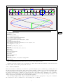
The new commands defined in the xpicture package and requiring some kind of coordinates support polar
coordinates, except the Picture and xpicture environments and the \cartesianaxes and \cartesiangrid
environments.
3.2
The Picture (or xpicture) environment
The xpicture package supports all drawing commands from standard LATEX; in particular, you can use the
picture environment. However, in the expression
\begin{picture}(x ,y )(x0 ,y0 )
the pairs of numbers (x,y ) and (x0,y0 ) always denote standard coordinates, namely, the picture environment only uses the standard reference, thus it defines, as drawing area, the rectangle [x0,x-x0 ]×[y0,y-y0 ],
regardless of whether this is the active reference. If we want draw a picture referring coordinates to an alternative reference system, to determine the appropriate drawing area in absolute coordinates is not obvious (and
often is difficult). However, the Picture environment defines a working area on the active reference system:
the
\begin{Picture}[color ](x0 ,y0 )(x1 ,y1 )
instruction fixes the drawing area [x0,x1 ]×[y0,y1 ], refered to the active reference system. Here, the (x0,y0 )
i (x1,y1 ) coordinates are always rectangular (even when reference in polar coordinates is active). More
precisely, this environment defines a picture box that circumscribes our drawing area. If the optional argument
is used, background is colored in the given color.
Very important: note that the syntax of the picture environment is not analogous to the new environment
Picture: Here two pairs of coordinates are required, (x0,y0 ) and (x1,y1 ), representing two opposite corners
of the drawing area.2 Obviously, if the reference sustem is the standard, expression
\begin{Picture}(0,0)(x ,y )
is equivalent to
\begin{picture}(x ,y )
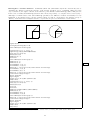
The following example shows the boxes produced by the picture and Picture environments.
2 Although it may seem more logical preserve the syntax of picture environment, it is more natural to define the drawing area
in that way.
6
Ex. 3
3
−3
2
−2
−1
3
−3
−1
2
−2
−2
1
−1
−3
1
2
3
−1
−2
1
1
Ex. 4
2
−3
3
\begin{center}
\setlength{\unitlength}{0.5cm}
\referencesystem(0,0)(1,-1)(1,1)
\fbox{\begin{picture}(6,6)(-3,-3)
\cartesiangrid(-3,-3)(3,3)
\end{picture}}\qquad
\fbox{\begin{Picture}(-3,-3)(3,3)
\cartesiangrid(-3,-3)(3,3)
\end{Picture}}
\end{center}
The left picture does not fit the box. In fact, some elementary geometric considerations shown that a square
box of 12 × 12 units of length must be reserved,
\begin{picture}(12,12)(-6,-6)
The use of the Picture environment frees us to determine the actual dimensions of the drawing.
The new environment xpicture is an alias to the Picture environment. Its sintax and its behavior are
identical.
On the other hand, the \draftPictures declaration disables all the instructions defined in this package,
replacing each picture set in a Picture environment by a parallelogram circumscribed by a white rectangle (the
box that shows the area reserved for the drawing).3
3.3
xpicture
xpicture
\standardreferencesystem
\referencesystem(0,0)(1,0)(0.5,1)
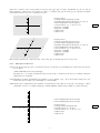
Coordinate axes
Instruction
\cartesianaxes(x0 ,y0 )(x1 ,y1 )
3 If
you use an instruction not directly defined by xpicture (inside of a Picture environment), this instruction may take effect.
7
draws the coordinate axes corresponding to the [x0,x1 ]×[y0,y1 ] rectangle. Arguments x0 , y0 , x1 and y1
must satisfy the conditions x0 <x1 and y0 <y1 . Here, coordinates (x0,y0 ) and (x1,y1 ) are always rectangular
(even when reference in polar coordinates is active).
y
2
1
x
−3
−2
−1
−1
1
2
3
−2
\begin{center}
\setlength{\unitlength}{0.75cm}%
\begin{Picture}[black!10!white](-4,-3)(4,3)
\renewcommand{\Pictlabelsep}{0.2}
\cartesianaxes(-3.5,-2.5)(3.5,2.5)
\Put[r](3.5,0){$x$}
\Put[t](0,2.5){$y$}
\end{Picture}
\end{center}
Ex. 5
\begin{center}
\referencesystem(0,0)(1,0)(0.5,1)
\setlength{\unitlength}{0.75cm}%
\begin{Picture}[black!10!white](-4,-3)(4,3)
\renewcommand{\Pictlabelsep}{0.2}
\cartesianaxes(-3.5,-2.5)(3.5,2.5)
\Put[r](3.5,0){$x$}
\Put[t](0,2.5){$y$}
\end{Picture}
\end{center}
Ex. 6
y
2
1
x
−3
−2
−1
−1
1
2
3
−2
The following parameters control the style of the axes, the cut marks and labels on the axes:
3.3.1
The style of the axes
\axescolor By default, the axes color is black, but we can change it by redefining the \axescolor declaration.
For example,
\renewcommand{\axescolor}{orange}
We must use a color name predefined in the package xcolor or defined by the user (for example, using the
\definecolor command).
\axesthickness Length determining the thickness of axes (default 1 pt). You can modify it using any command that fixes a length (as \setlength or \settowidth).
\xunitdivisions, \yunitdivisions Number of subdivisions of the unit (in each axis). By default, 1. These
arguments can also be redefined using the \renewcommand command (they must be positive integers).
3
2
\renewcommand{\xunitdivisions}{2}
\renewcommand{\yunitdivisions}{3}
1
−3
−2
−1
1
2
\begin{center}
\setlength{\unitlength}{1cm}%
\begin{Picture}(-4,-4)(4,4)
\cartesianaxes(-3.5,-3.5)(3.5,3.5)
\end{Picture}
\end{center}
3
−1
−2
−3
8
Ex. 7
3.3.2
Axes position
The coordinate axes (and also tags and cut marks) are placed by default in the traditional way, on the y = 0
(the x axis) and x = 0 (the y axis) lines. However, sometimes the fact that labels are inside the graphic can be
annoying.4 Alternatively, we can place axes and tags at the lower and left sides of the coordinate rectangle. To
choose between these two options we should use the following declarations:
\internalaxes, \externalaxes If the \internalaxes declaration is active, then axes lies on y = 0 and x = 0.
However, if we activate the \externalaxes declaration, the axes produced by the instruction
\cartesianaxes(x0 ,y0 )(x1 ,y1 )
lies on y = y0 and x = x0 .
By default, the \internalaxes declaration is active.
3
2
\renewcommand{\xunitdivisions}{2}
\renewcommand{\yunitdivisions}{2}
1
\begin{center}
\externalaxes
\setlength{\unitlength}{1cm}%
\begin{Picture}(-4,-4)(4,4)
\cartesianaxes(-3.5,-3.5)(3.5,3.5)
\end{Picture}
\end{center}
0
−1
−2
−3
−3
3.3.3
−2
−1
0
1
2
3
Tags style
The numerical tags on the axes are made in math mode. If you need textual labels, put them in a \mbox
or, using amsmath, a \text box. We can control the color, attributes and distance to the axes of these tags,
redefining (with \renewcommand) the following marks:
\axeslabelcolor The color of the numerical tags on the axes. By default, this color is identical to the axes
color.
\axeslabelsize Size of numerical tags. By default, \small.
\axeslabelmathversion Mathversion of numerical tags. By default, normal.5
\axeslabelmathalphabet Mathalphabet of numerical tags. By default, \mathrm.
\axislabelsep Distance between tags and cut marks, measured in \unitlength units;6 by default, 0.1 (see
later the description of \makenotics).
3.3.4
Tags position
Position of tags is controlled by two declarations:
\xlabelpos{position } change the relative position of labels in x axis. Admissible values are those allowed in
the position argument of command \Put (see subsection 4.1). Default is -90.
\ylabelpos{position } change the relative position of labels in y axis. Default is 180.
4 And
produces strange effects when the origin (0.0) is not in the drawing area.
math versions are normal and bold, but some packages define other math versions.
6 The distance between axes and tags equals \ticssize+\axislabelsep.
5 Standard
9
Ex. 8
3.3.5
Style of cut marks
Units (and, optionally, unit fractions) are marked over axes with small segments, the style of which is controlled
by the following parameters:
\ticssize, \secundaryticssize These lengths control the size of the tics: \ticssize is half the length of
main cuts (by default, 4pt) and \secundaryticssize is half the length of secundary cuts (by default,
2pt).
\ticsthickness Thickness of the marks on axes (by default, 1pt).
\ticscolor Color of the marks on axes (by default, black).
\renewcommand{\axescolor}{blue}
\setlength{\axesthickness}{3pt}
\renewcommand{\xunitdivisions}{2}
\renewcommand{\yunitdivisions}{3}
−4
\renewcommand{\axeslabelcolor}{teal}
\renewcommand{\axeslabelsize}{\footnotesize}
\renewcommand{\axeslabelmathversion}{bold}
\renewcommand{\axeslabelmathalphabet}{\mathsf}
\renewcommand{\axislabelsep}{0.05}
\xlabelpos{ttl}
\ylabelpos{r}
3
−3
2
−2
−1
1
1
\setlength{\ticssize}{0.2cm}
\setlength{\secundaryticssize}{0.1cm}
\setlength{\ticsthickness}{2pt}
\renewcommand{\ticscolor}{blue!50}
2
−1
3
4
−2
−3
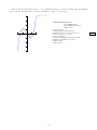
3.3.6
Ex. 9
\begin{center}
\degreesangles
\rotateaxes{-30}
\setlength{\unitlength}{0.75cm}%
\begin{Picture}(-5,-4)(5,4)
\cartesianaxes(-4.5,-3.5)(4.5,3.5)
\end{Picture}
\end{center}
Removing and directly printing cut marks and labels
\maketics, \makenotics These two declarations determine if divisions on the axes should be marked or not.
By default the \maketics declaration is active.
If divisions are not marked, the \axislabelsep declaration determines the distance between axes and
labels.
2
\begin{center}
\setlength{\unitlength}{0.75cm}%
\begin{Picture}(-4.5,-2.5)(4.5,2.5)
\makenotics
\cartesianaxes(-4,-2)(4,2)
\end{Picture}
\end{center}
1
−4
−3
−2
−1
1
2
3
4
−1
−2
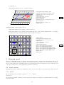
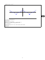
\makelabels, \makenolabels Two declarations determining whether numerical labels on the axes must appear
or not. By default, the \makelabels declaration is active.
10
Ex. 10
\begin{center}
\setlength{\unitlength}{0.75cm}%
\begin{Picture}(-4.5,-2.5)(4.5,2.5)
\makenolabels
\cartesianaxes(-4,-2)(4,2)
\end{Picture}
\end{center}
Ex. 11
Declarations \makenotics and \makenolabels can be useful when you want to show only some specific
coordinates, when the points to be highlighted on the axes are not integers and when you need to print labels
in some special format. In this cases you can plot tics and/or print labels using the following commands.
\plotxtic{x-coor }, \plotytic{y-coor } plot a tic for the given x or y coordinate.
\printxlabel{x-coor }{label }, \printylabel{y-coor }{label } print label for the given x or y coordinate.
Labels are printed in math mode.
\printxticlabel{x-coor }{label }, \printyticlabel{y-coor }{label } plot a tic and print label for the
given x or y coordinate.
\begin{center}
\setlength{\unitlength}{1cm}%
\begin{Picture}(-4.5,-0.5)(4.5,3.5)
\makenolabels
\makenotics
\cartesianaxes(-4,0)(4,3)
\plotytic{0.5}
\printylabel{0.5}{1/2}
\printxticlabel{2}{2}
1/2
\Polyline(2,0)(2,0.5)(0,0,5)
\thicklines
\SCALEfunction{0.125}{\SQUAREfunction}{\F}
\PlotFunction[3]{\F}{-4}{4}
\end{Picture}
\end{center}
2
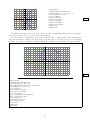
Multiple equally spaced tics and/or labels can be drawn simultaneously:
\plotxtics{firstcoor }{incr }{bound }, \plotytics{firstcoor }{incr }{bound } plot several (x or y) tics,
from the initial coordinate firstcoor ; incr is the distance between consecutive tics, and the last tic is not
in a position greater than bound.
\printxlabels[digits ]{firstcoor }{incr }{bound }, \printylabels[digits ]{firstcoor }{incr }{bound }
print several labels, from the initial coordinate firstcoor ; incr is the distance between consecutive label
positions, and the last position is not greater than bound. The optional argument digits is the number of
decimal digits to be printed (by default, numbers are printed with its natural number of decimals).
\printxticslabels[digits ]{firstcoor }{incr }{bound } plot x tics and labels simultaneously.
\printyticslabels[digits ]{firstcoor }{incr }{bound } plot y tics and labels simultaneously.
11
Ex. 12
\externalaxes
\setlength{\unitlength}{1cm}
\renewcommand{\axeslabelsize}{\tiny}
\referencesystem(0,0)(1.5,0)(0,2)
\begin{center}
\begin{Picture}(-2.5,-1.5)(2.5,1.5)
\makenotics
\makenolabels
\cartesianaxes(-2.25,-1.25)(2.25,1.25)
\printxticslabels[1]{-2}{0.5}{2.25}
\printyticslabels[4]{-1}{0.25}{1}
\end{Picture}
\end{center}
1.0000
0.7500
0.5000
0.2500
0.0000
−0.2500
−0.5000
−0.7500
−1.0000
−2.0
−1.5
−1.0
−0.5
0.0
0.5
1.0
1.5
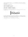
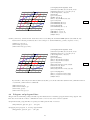
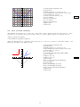
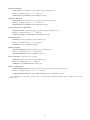
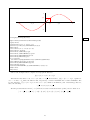
Ex. 13
2.0
2
1.5
1
0.5
−2π
−3π/2
−π
−π/2 −0.5
π/2
π
3π/2
2π
−1
−1.5
−2
\setlength{\unitlength}{1cm}
\begin{center}
\begin{Picture}(-7,-2.5)(7,2.5)
{\referencesystem(0,0)(\numberHALFPI,0)(0,1)
\renewcommand{\xunitdivisions}{2}
\renewcommand{\yunitdivisions}{2}
\makenolabels
\renewcommand{\Pictlabelsep}{0.25}
\cartesianaxes(-4.2,-2.2)(4.2,2.2)
Ex. 14
\printylabels{-2}{0.5}{2}
\highestlabel{$-3\pi/2$}
\printxlabel{-4}{-2\pi}
\printxlabel{-3}{-3\pi/2}
\printxlabel{-2}{-\pi}
\printxlabel{-1}{-\pi/2}
\printxlabel{1}{\pi/2}
\printxlabel{2}{\pi}
\printxlabel{3}{3\pi/2}
\printxlabel{4}{2\pi}
}
\end{Picture}
\end{center}
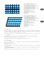
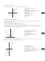
3.4
Cartesian grids
As an alternative to the \cartesianaxes command, we can use \cartesiangrid, to better visualize the coordinates:
\cartesiangrid(x0, y0)(x1, y1)
12
2
1
−3
−2
−1
1
2
3
−1
−2
2
1
0
−1
−2
−3
3.4.1
−2
−1
0
1
2
3
\definecolor{myblue}{cmyk}{1,1,0,0.5}
\renewcommand{\gridcolor}{myblue}
\renewcommand{\secundarygridcolor}{cyan}
\setlength{\gridthickness}{0.5pt}
\setlength{\secundarygridthickness}{0.1pt}
\renewcommand{\xunitdivisions}{5}
\renewcommand{\yunitdivisions}{5}
\renewcommand{\axeslabelsize}{\footnotesize}
\begin{center}
\setlength{\unitlength}{1cm}
\begin{Picture}(-3.5,-2.5)(3.5,2.5)
\cartesiangrid(-3.4,-2.4)(3.4,2.4)
\end{Picture}
\end{center}
Ex. 15
\definecolor{myblue}{cmyk}{1,1,0,0.5}
\renewcommand{\gridcolor}{myblue}
\renewcommand{\secundarygridcolor}{cyan}
\setlength{\gridthickness}{0.5pt}
\setlength{\secundarygridthickness}{0.1pt}
\renewcommand{\xunitdivisions}{5}
\renewcommand{\yunitdivisions}{5}
\renewcommand{\axeslabelsize}{\footnotesize}
\begin{center}
\setlength{\unitlength}{1cm}
\referencesystem(0,0)(1,0)(0.25,1)
\externalaxes
\begin{Picture}(-4,-3)(4,3)
\cartesiangrid(-3.4,-2.4)(3.4,2.4)
\end{Picture}
\end{center}
Ex. 16
Grid style
Note that, in addition to the parameters outlined above, there are the following ones, which control the style
of the grid (as in previous cases, these parameters are changed by redefining them with the \renewcommand
declaration, or using the usual instructions when they are lengths).
\gridcolor determines the color of main divisions in the grid (regardless of the axes color). By default, this
color is gray.
\secundarygridcolor determines the color of secundary divisions in the grid. By default, lightgray).
\gridthickness thickness of main divisions (by default, 0.4pt).
\secundarygridthickness thickness of secundary divisions (by default, 0.2pt).
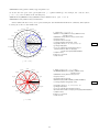
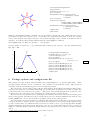
3.5
Polar grids
Finally, instead of Cartesian axes, we can construct a polar grid (obviously, this option will be interesting when
we use polar coordinates).
\polargrid{radius }{circledivs }
(radius and circledivs are, respectively, the radius and the number of divisions of the circle (circledivs must
be a positive integer).
This command supports the same parameters that \cartesianaxes and \cartesiangrid (when they makes
sense), and also the following:
\runitdivisions Number of radial subdivisions of the unit. By default, 1 (it must be a positive integer).
13
π/2
2π/3
π/3
5π/6
π/6
π
1
2
3
7π/6
0
11π/6
4π/3
\renewcommand{\runitdivisions}{2}
\setlength{\unitlength}{0.75cm}
\renewcommand{\gridcolor}{magenta}
\begin{center}
\begin{Picture}(-4,-4)(4,4)
\polargrid{3.5}{12}
\end{Picture}
\end{center}
Ex. 17
\renewcommand{\runitdivisions}{2}
\setlength{\unitlength}{0.75cm}
\renewcommand{\gridcolor}{magenta}
\referencesystem(0,0)(1,-1)(0.5,0.5)
\begin{center}
\begin{Picture}(-3.5,-3.5)(3.5,3.5)
\polargrid{3.5}{12}
\end{Picture}
\end{center}
Ex. 18
5π/3
3π/2
5π/6
π
2π/3
7π/6
π/2
4π/3
π/3
1
3π/2
2
π/6
3
5π/3
0
11π/6
\degreespolarlabels, \radianspolarlabels Arcs are printed, by default, in radians. If you want angular
units mesured in degrees, use the \degreespolarlabels declaration (obviously, \radianspolarlabels
recovers tags in radians).
o
105o
90o
75o
120
60o
135o
45o
150o
30o
165o
\begin{center}
\degreespolarlabels
\setlength{\unitlength}{1cm}
\begin{Picture}(-4,-4)(4,4)
\polargrid{3}{24}
\end{Picture}
\end{center}
15o
180o
1
0o
3
2
195o
345o
210o
330o
225o
315o
240o
255o 270o 285o
300o
14
Ex. 19
\rlabelpos Relative position of labels in polar axis. Admissible values are those allowed in the position
argument of command \Put (see subsection 4.1). Default is bbr.
3π/5
2π/5
4π/5
π/5
π
1
2
6π/5
3
\begin{center}
\setlength{\unitlength}{1cm}
\begin{Picture}(-4,-4)(4,4)
\rlabelpos{b}
\polargrid{3.5}{10}
\end{Picture}
\end{center}
0
Ex. 20
9π/5
7π/5
8π/5
To remove tags on the polar axis and angles you can use the \makenolabels declaration.
4
Alternatives to standard commands \put,\multiput, \line, and \vector
Standard commands used inside the picture environment are not modified by this package (although if we
include these commands in the body of a Picture environment). In particular, there does not affect the
\referencesystem declaration. This package introduces similar commands to those which are sensitive to the
active reference system and give us a greater control over their behavior. These are the instructions described
below.
4.1
Extensions of the \put command
\Put, \cPut, \rPut
\Put[position ](x ,y ){object }
\Put*[position ](x ,y ){object }
\cPut{position }(x ,y ){object }
\rPut{position }(x ,y ){object }
\rPut*{position }(x ,y ){object }
place the drawing pointer in the point of coordinates (x ,y ) with respect to the active reference system
(which may coincide or not with the standard system). These commands differ in the criteria used to
determine the precise position of the object.
Involved parameters are (see below)
\Pictlabelsep{distance }
\defaultPut{c}/\defaultPut{r}
\highestlabel{text }
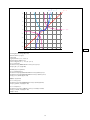
In the following example, the red circle (included as an argument in the \put command) is at the point
of standard coordinates (1, −1); however, in the case of the blue circle, coordinates (1, −1) refer to the
active reference system.
15
\begin{center}
\setlength{\unitlength}{0.75cm}
\referencesystem(0,0)(1,-1)(1,1)
\begin{Picture}(-2.5,-2.5)(2.5,2.5)
\cartesiangrid(-2,-2)(2,2)
\pictcolor{red}
\put(1,-1){\circle*{0.25}}
\pictcolor{blue}
\Put(1,-1){\circle*{0.25}}
\end{Picture}
\end{center}
2
−2
1
−1
−1
1
−2
2
Ex. 21
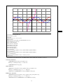
Recall that coordinates can be rectangular or polar, and angles may be measured in radians or in degrees.
\begin{center}
\setlength{\unitlength}{1cm}
\begin{Picture}(-2.5,-2.5)(2.5,2.5)
\cartesiangrid(-2,-2)(2,2)
\polarreference
\pictcolor{blue}
\Put(1,\numberHALFPI){\circle*{0.25}}
\degreesangles
\pictcolor{red}
\Put(1,180){\circle*{0.25}}
\end{Picture}
\end{center}
2
1
−2
−1
1
2
−1
−2
4.1.1
Accurate positioning of the graphical object
The position argument allows us to fix the relative position of object respect to point (x,y ). Note that
this argument is optional in \Put and \Put*, but mandatory in the other commands we are describing.
The purpose of this parameter is to rationalize the disposition of objects, especially when they are not
strictly graphical objects (but labels, text boxes or mathematical formulas). In these cases, the appropriate
choice of coordinates seems a problem that is not well solved with standard instructions, despite the special
syntax of the \makebox command in the picture environment. For example, in this picture (which we
made using only the standard LATEX commands)
cos x
1
sin x
0
π
π/2
−1
16
3π/2
2π
Ex. 22
we have located numerical labels (0, 1, π. . . ) at 0.15\unitlength of its natural position over the axes,
while the reference points of tags “sin x” and “cos x” are just in points (3π/4, sin(3π/4)) and (2π, 1), using
these instructions:
\put(2.356194,0.707107){$\sin x$}
\put(6.283185,1){$\cos x$}
\put(-0.15,-1){\makebox(0,0)[r]{$-1$}}
\put(-0.15,0){\makebox(0,0)[r]{$0$}}
\put(-0.15,1){\makebox(0,0)[r]{$1$}}
\put(1.570796,-0.15){\makebox(0,0)[t]{$\pi/2$}}
\put(3.141593,-0.15){\makebox(0,0)[t]{$\pi$}}
\put(4.712389,-0.15){\makebox(0,0)[t]{$3\pi/2$}}
\put(6.283185,-0.15){\makebox(0,0)[t]{$2\pi$}}
If we change the value of \unitlength, then these values become inappropriate and we need to change
several lines of code.
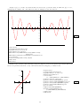
1
0
cos x
sin x
π
π/2
3π/2
2π
−1
Note that, regarding labels along the x axis, instead of aligning them to a fixed distance of this axis,
there would be better to align the baselines (π and 2π should go down); some of these labels should move
slightly to the right or to the left to avoid that it cut the graph. Finally, the tag “cos x” should be vertically
centered (with respect to the curve) and slightly moved to the right.
Using the xpicture package we construct this picture in the following way:
17
1
cos x
sin x
0
π/2
π
3π/2
2π
−1
\MULTIPLY{3}{\numberQUARTERPI}{\numberTQPI}
\SIN{\numberTQPI}{\sinTQPI}
\begin{center}
\setlength{\unitlength}{2cm}
\begin{Picture}(-0.5,-1.5)(6.5,1.5)
{\referencesystem(0,0)(\numberHALFPI,0)(0,1)
\makenolabels
\renewcommand{\Pictlabelsep}{0.1}
\highestlabel{$-3\pi/2$}
\cartesianaxes(0,-1.5)(4.25,1.5)
Ex. 23
\rPut{l}(0,-1){$-1$}
\rPut{l}(0,0){$0$}
\rPut{l}(0,1){$1$}
\rPut*{bbl}(1,0){$\pi/2$}
\rPut*{b}(2,0){$\pi$}
\rPut*{bbr}(3,0){$3\pi/2$}
\rPut*{b}(4,0){$2\pi$}
% put the y-axis labels at left
%
%
%
%
put
put
put
put
"\pi/2" at bbl
"\pi" at bottom
"3\pi/2" at bbr
"2\pi" at bottom
\rPut*{b}(0,0){\pictcolor{gray}\xLINE(0.75,0)(4.25,0)}} % \baseline of x-labels
\PlotFunction[8]{\COSfunction}{0}{\numberTWOPI}
\PlotFunction[8]{\SINfunction}{0}{\numberTWOPI}
\Put[NE](\numberTQPI,\sinTQPI){$\sin x$}
\Put[E](\numberTWOPI,1){$\cos x$}
\end{Picture}
\end{center}
% put "\sin x" at NorthEast
% put "\cos x" at East
Here we used several tools to draw the graphs of the functions. But aside from this, commands \Put,
\rPut and \rPut* have allowed we to determine the logical position of objects in a much more reasonable
way.7
Argument position supports multiple values:
An integer or decimal number, determining the angle (in degrees) where object is placed, with respect to the reference point (x,y ).
7 Regarding to labels on coordinated axes a better choice would be to use other specific commands, as \printxlabels. Here we
have chosen \rPut because we are illustrating this instruction.
18
0
45
90 135
180
225
270
315
360
\begin{center}
\setlength{\unitlength}{1cm}
\begin{Picture}(0,-1)(9,1)
\makenolabels
\renewcommand{\axescolor}{lightgray}\renewcommand{\ticscolor}{lightgray}
\cartesiangrid(0,-1)(8,1)
\pictcolor{blue}
\Put[0](0,0){0}
\Put[45](1,0){45}
\Put[90](2,0){90}
\Put[135](3,0){135}
\Put[180](4,0){180}
\Put[225](5,0){225}
\Put[270](6,0){270}
\Put[315](7,0){315}
\Put[360](8,0){360}
\end{Picture}
\end{center}
Ex. 24
Letter c (from center ), which places the center of object at point (x ,y ).
1
\begin{center}
\setlength{\unitlength}{2cm}
\begin{Picture}(-1,-1)(1,1)
\cartesianaxes(-1,-1)(1,1)
\pictcolor{blue}
\Put[c](0,0){A CENTERED BOX}
\end{Picture}
\end{center}
A CENTERED BOX
−1
1
Ex. 25
−1
Note that this option is not equivalent to the suppression of the optional argument, because in that case
the reference point of object is located in (x ,y ).
1
A NONCENTERED BOX
−1
1
\begin{center}
\setlength{\unitlength}{2cm}
\begin{Picture}(-1,-1)(1,1)
\cartesianaxes(-1,-1)(1,1)
\pictcolor{blue}
\Put(0,0){A NONCENTERED BOX}
\end{Picture}
\end{center}
−1
Letters or letter combinations N, E, S, W, NE, SE, SW, NW, NNE, ENE, ESE, SSE, SSW, WSW, WNW, NNW
Abbreviation of North, East. . . , North-East. . . , North-North-East. . .
For example, the
\Put[NE](0,0){A}
instruction writes “A” at north-east of point (0,0).
Letters o letter combinations t, r, b, l, tr, br, bl, tl, ttr, rtr, rbr, bbr, bbl, lbl, ltl, ttl
Abbreviation of top, right. . . , top-right. . . , top-top-right. . .
For example,
19
Ex. 26
\Put[tr](0,0){A}
writes “A” at top and right of point (0,0).
Parameter \Pictlabelsep determines the distance between the graphical object and the given point.
In the following examples we have made this argument very big to clearly appreciate the positioning
of objects.
\renewcommand{\Pictlabelsep}{1}
\begin{center}
\setlength{\unitlength}{2.5cm}%
NNW
N
\begin{Picture}(-1.5,-1.5)(1.5,1.5)
\Put[N](0,0){N}
\Put[S](0,0){S}
\Put[E](0,0){E}
\Put[W](0,0){W}
\Put[NE](0,0){NE}
\Put[SE](0,0){SE}
\Put[SW](0,0){SW}
\Put[NW](0,0){NW}
%
\Put[NNE](0,0){NNE}
\Put[ENE](0,0){ENE}
\Put[ESE](0,0){ESE}
\Put[SSE](0,0){SSE}
\Put[SSW](0,0){SSW}
\Put[WSW](0,0){WSW}
\Put[WNW](0,0){WNW}
\Put[NNW](0,0){NNW}
\Put(0,0){\Circle{1}}
\xLINE(-1,0)(1,0)
\xLINE(0,-1)(0,1)
\end{Picture}
\end{center}
NNE
NW
NE
WNW
ENE
W
E
WSW
ESE
SW
SE
SSW
S
SSE
Ex. 27
\renewcommand{\Pictlabelsep}{1}
\begin{center}
\setlength{\unitlength}{2.5cm}%
tl
ttl
t
ttr
tr
rtr
ltl
r
l
lbl
bl
\begin{Picture}(-1.5,-1.5)(1.5,1.5)
\Put[t](0,0){t}
\Put[r](0,0){r}
\Put[b](0,0){b}
\Put[l](0,0){l}
\Put[tr](0,0){tr}
\Put[br](0,0){br}
\Put[bl](0,0){bl}
\Put[tl](0,0){tl}
\Put[ttr](0,0){ttr}
\Put[rtr](0,0){rtr}
\Put[rbr](0,0){rbr}
\Put[bbr](0,0){bbr}
\Put[bbl](0,0){bbl}
\Put[lbl](0,0){lbl}
\Put[ltl](0,0){ltl}
\Put[ttl](0,0){ttl}
\Put(0,0){%
\regularPolygon[45]{\numberSQRTTWO}{4}}
\xLINE(-1,0)(1,0)
\xLINE(0,-1)(0,1)
\end{Picture}
\end{center}
rbr
bbl
b
bbr
br
20
Ex. 28
Rectangular o circular distance? Commands \rPut and \cPut differ only in the criterion they use to
determine the distance between the reference point and the graphical object. Command \rPut places the
object (outside of) the square centered at the reference point and side 2\Pictlabelsep, while \cPut places it
in the cercle of radius \Pictlabelsep (letters r and c mean, respectively, a rectangular and circular layout).8
Although, for small values of the \Pictlabelsep parameter, the difference is subtle and usually not very
significant, it is generally best to use the circular version (because it corresponds to the natural concept of
distance) and reserve the rectangular version to objects that are placed on horizontal or vertical lines.
r
c
45o
45o
\Pictlabelsep
\Pictlabelsep
\Pictlabelsep
\begin{center}
\setlength{\unitlength}{1.5cm}
\renewcommand{\Pictlabelsep}{1}
\begin{Picture}(-1.5,-1.5)(2,1.5)
\regularPolygon[45]{\numberSQRTTWO}{4}
\Put(0,0){\circle*{0.1}}
\rPut{45}(0,0){r}
\xLINE(0,0)(0,-1)
\thicklines
\renewcommand{\Pictlabelsep}{0.1}
\xLINE(0,0)(1,1)
\xLINE(0,0)(1,0)
\xtrivVECTOR(0,-1)(1,-1)
\xtrivVECTOR(1,-1)(0,-1)
\rPut{b}(0.5,-1){\footnotesize\textbackslash Pictlabelsep}
\xtrivVECTOR(1,-1)(1,0)
\xtrivVECTOR(1,0)(1,-1)
\rPut{r}(1,-0.5){\footnotesize\textbackslash Pictlabelsep}
\polarreference\degreesangles
\xArc{0.3}{0}{45}
\degreesangles
\Put[22.5](0.3,22.5){$45^{\mathrm o}$}
\end{Picture}
\begin{Picture}(-1.5,-1.5)(2,1.5)
\Put(0,0){\circle*{0.1}}
\cPut{45}(0,0){c}
\Circle{1}
\thicklines
\xLINE(0,0)(\numberCOSXLV,\numberCOSXLV)
\xLINE(0,0)(1,0)
\xtrivVECTOR(0,0)(0,-1)
\xtrivVECTOR(0,-1)(0,0)
\renewcommand{\Pictlabelsep}{0.1}
\rPut{r}(0,-0.5){\footnotesize\textbackslash Pictlabelsep}
\polarreference\degreesangles
\xArc{0.3}{0}{45}
\degreesangles
\Put[22.5](0.3,22.5){$45^{\mathrm o}$}
\end{Picture}
\end{center}
8 For
the mathematicians: command \cPut uses the euclidean norm (or 2-norm), while \rPut uses the infinite norm.
21
Ex. 29
Note that if the commands we use are \rPut or \cPut, then the positioners t, r, tr. . . are equivalent to the
corresponding N, E, NE. . . However, the \Put command choose between rectangular or circular layout following
this criteria:
• Positioners of compass type (like NE) use the circular layout.
• Positioners t, tr, et cetera use the rectangular layout.
• If the positioner is an angle (a number), it uses a default position which is set using the \defaultPut
declaration: \defaultPut{c} determines a circular distance, while \defaultPut{r} determines the rectangular alternative.
\renewcommand{\Pictlabelsep}{1}
\begin{center}
\setlength{\unitlength}{2.5cm}%
r
c
\begin{Picture}(-1.5,-1.5)(1.5,1.5)
\defaultPut{c}
\Put[45](0,0){c}
\defaultPut{r}
\Put[45](0,0){r}
\regularPolygon[45]{\numberSQRTTWO}{4}
\Put(0,0){\Circle{1}}
\xLINE(-1,0)(1,0)
\xLINE(0,-1)(0,1)
\end{Picture}
\end{center}
Ex. 30
Alignment by the baseline Starred versions \Put* and \rPut* allow us to align by the baseline objects
positioned below the reference point. To use these commands, user must decide which is the higher object to
be positioned, and introduce it as an argument of the \highestlabel declaration. For example, typing
\highestlabel{\Huge A}
A
we reserve a sufficient vertical space to write the character
.
It should be noted that starred versions behave differently only when the position of the object stands under
the reference point, with positioners bbl, b or bbr, or with an appropiate angle (as -90 or 300); otherwise
(including S, SSW, et cetera), the \Put* and \rPut* commands are equivalent to the non-starred commands
\Put and \rPut.
\begin{center}
\setlength{\unitlength}{1cm}
A
A
A
A
A
\begin{Picture}(-3.5,-1.5)(3.5,1.5)
\xLINE(-3.5,0)(3.5,0)
\multiPut(-3,-0.1)(1,0){7}{\xLINE(0,0)(0,0.2)}
\highestlabel{\Huge A}
\renewcommand{\Pictlabelsep}{0.2}
\Put*[bbl](-3,0){\small A}
\Put*[b](-2,0){\normalsize A}
\Put*[-100](-1,0){\large A}
\Put*[-90](0,0){\Large A}
\Put*[270](1,0){\LARGE A}
\Put*[300](2,0){\huge A}
\Put*[bbr](3,0){\Huge A}
\Put*[bbl](-3.5,0){%
\pictcolor{gray}\xLINE(0,0)(7,0)}
\end{Picture}
\end{center}
A A
When a Picture environment starts, highest label is set to \normalfont\normalsize$1$ (i.e., the high of
a normal 1).
22
Ex. 31
4.2
Alternatives to the \multiput command
The xpicture package introduces two families of commands to generalize the \multiput command:
1. The natural generalization, with all versions,
\multiPut[position ](x0 ,y0 )(∆x ,∆y ){n }{object }
\multiPut*[position ](x0 ,y0 )(∆x ,∆y ){n }{object }
\multicPut{position }(x0 ,y0 )(∆x ,∆y ){n }{object }
\multirPut{position }(x0 ,y0 )(∆x ,∆y ){n }{object }
\multirPut*{position }(x0 ,y0 )(∆x ,∆y ){n }{object }
These commands compose n copies of object in (x0, y0), (x0 + ∆x, y0 + ∆y), (x0 + 2∆x, y0 + 2∆y),. . . ,
(x0 + (n − 1)∆x, y0 + (n − 1)∆y).
2. A new command group,
\multiPlot[position ]{object }(x0 ,y0 )(x1 ,y1 )...(xn ,yn )
\multiPlot*[position ]{object }(x0 ,y0 )(x1 ,y1 )...(xn ,yn )
\multicPlot{position }{object }(x0 ,y0 )(x1 ,y1 )...(xn ,yn )
\multirPlot{position }{object }(x0 ,y0 )(x1 ,y1 )...(xn ,yn )
\multirPlot*{position }{object }(x0 ,y0 )(x1 ,y1 )...(xn ,yn )
These commands compose the done object in several positions, that are freely entered as a list of coordinate
pairs.
2
\begin{center}
\setlength{\unitlength}{1cm}
\referencesystem(0,0)(1,-1)(1,1)
\begin{Picture}(-2.5,-2.5)(2.5,2.5)
\cartesiangrid(-2,-2)(2,2)
\pictcolor{blue}
\multiPut(-2,-2)(1,1){5}{\circle*{0.25}}
\pictcolor{red}
\multiPlot{\circle*{0.25}}(-1,-2)(2,1)(-2,2)
\end{Picture}
\end{center}
−2
1
−1
−1
1
−2
2
23
Ex. 32
2
\begin{center}
\setlength{\unitlength}{1cm}
\referencesystem(0,0)(1,-1)(1,1)
\begin{Picture}(-2.5,-2.5)(2.5,2.5)
\cartesiangrid(-2,-2)(2,2)
Ex. 33
\pictcolor{blue}
\multiPut[b](-2,-2)(1,1){5}{\circle*{0.25}}
\pictcolor{red}
\multiPlot[NE]{\circle*{0.25}}(-1,-2)(2,1)(-2,2)
\end{Picture}
\end{center}
−2
1
−1
−1
1
−2
2
4.3
Alternatives to \line and \vector
\xLINE This command draws line segments:
\xLINE(x0 ,y0 )(x1 ,y1 )
draws the line segment between the two points (x0 ,y0 ) and (x1 ,y1 ) (Cartesian or polar coordinates, in
the active reference system). This allows us to draw any segment in any direction.
\xVECTOR, \xtrivVECTOR plot arrows:
\xVECTOR(x0 ,y0 )(x1 ,y1 )
\xtrivVECTOR(x0 ,y0 )(x1 ,y1 )
draw an arrow between points (x0 ,y0 ) and (x1 ,y1 ). The \xtrivVECTOR command draw an arrow the
end of which simply consists of a pair of segments ( ). length and aperture of the end of arrow are
controled by the instruction
\arrowsize{xlen }{ylen }
where the two parameters are non-negative numbers: the first one for the length (in points); second for
the half of the aperture. Default is
\arrowsize{5}{2}
24
4
3
2
1
−4
−3
−2
−1
−1
1
2
3
4
−2
−3
−4
\setlength{\unitlength}{0.75cm}
\referencesystem(0,0)(1,0)(0.25,0.75)
\begin{Picture}(-4.5,-4.5)(4.5,4.5)
\cartesiangrid(-4,-4)(4,4)
\thicklines
\pictcolor{blue}
\xLINE(-4,0)(1,4)
\Put(1,-3){\xLINE(0,0)(3,2)}
\pictcolor{red}
\xtrivVECTOR(0,0)(2,3)
\xtrivVECTOR(0,0)(2,0)
\arrowsize{10}{4}
\xtrivVECTOR(0,0)(-2,-1)
Ex. 34
\pictcolor{magenta}
\xVECTOR(-3,-3)(-3,3)
\xVECTOR(-3,-3)(-2,-2)
\end{Picture}
\xline, \xvector, \xtrivvector draw lines and vectors using the standard LATEX syntax (but without any
restriction in allowed parameters, that can be integer or decimal numbers, positive, negative or zero).
\xline(x ,y ){size }
\xvector(x ,y ){size }
\xtrivvector(x ,y ){size }
4
3
2
1
−4
−3
−2
−1
−1
1
2
3
4
−2
−3
−4
\setlength{\unitlength}{0.75cm}
\referencesystem(0,0)(1,0)(0.25,0.75)
\begin{Picture}(-4.5,-4.5)(4.5,4.5)
\cartesiangrid(-4,-4)(4,4)
\thicklines
\pictcolor{blue}
\Put(-4,0){\xline(5,4){5}}
\Put(1,-3){\xline(3,2){3}}
\pictcolor{red}
\Put(0,0){\xtrivvector(2,3){2}}
\xtrivvector(1,0){2}
\arrowsize{10}{4}
\Put(0,0){\xtrivvector(2,1){-2}}
Ex. 35
\pictcolor{magenta}
\Put(-3,-3){\xvector(0,1){6}}
\Put(-3,-3){\xvector(1,1){1}}
\end{Picture}
If you want to draw only an arrowhead (without any line) you can use either the \zerovector/\zerotrivvector
or \xvector/\xtrivvector commands:
\zerovector(x ,y )
\zerotrivvector(x ,y )
\xvector(x ,y ){0}
\xtrivvector(x ,y ){0}
4.4
Polygons anf polygonal lines
The pict2e and curve2e packages include specific instructions for drawing polygonal lines and polygons. We
introduce new versions of these commands in order to refer to the active reference system.
\Polyline draws polygonal lines. Logically, we must pass the list of vertices:
\Polyline(x0 ,y0 )(x1 ,y1 )...(xn ,yn )
\Polygon plots polygons, ie, closed polygonal lines:
\Polygon(x0 ,y0 )(x1 ,y1 )...(xn ,yn )
25
is equivalent to
\Polyline(x0 ,y0 )(x1 ,y1 )...(xn ,yn )(x0 ,y0 )
4
\setlength{\unitlength}{0.75cm}
\referencesystem(0,0)(1,0)(0.25,0.75)
\begin{Picture}(-4.5,-4.5)(4.5,4.5)
\externalaxes
\cartesiangrid(-4,-4)(4,4)
\linethickness{1pt}
\pictcolor{blue}
\Polyline(-2,2)(-3,-1)(0,0)(2,3)(2,2)
\pictcolor{red}
\Polygon(0,0)(1,1)(3,1)(1,-1)
\end{Picture}
3
2
1
0
−1
−2
−3
−4
−4
−3
−2
−1
0
1
2
3
Ex. 36
4
\regularPolygon draws regular polygons:
\regularPolygon[initial angle ]{radius }{sides }
makes the regular polygon with the given radius and sides. The optional argument (zero, by default)
determines the slope of the first vertex, always measured in degrees.
7
6
\begin{center}
\setlength{\unitlength}{0.5cm}
\begin{Picture}(-7.5,-7.5)(7.5,7.5)
\externalaxes
\cartesiangrid(-7,-7)(7,7)
\pictcolor{blue}
\regularPolygon{1}{5}
\Put(-4,0){\regularPolygon{2}{6}}
\Put(3,3){\regularPolygon{2}{4}}
\Put(-4,-4){\regularPolygon[45]{2}{4}}
\Put(4,-4){\regularPolygon[90]{2.5}{11}}
\Put(-4,4){\regularPolygon[90]{3}{3}}
\end{Picture}
\end{center}
5
4
3
2
1
0
−1
−2
−3
−4
−5
−6
−7
−7 −6 −5 −4 −3 −2 −1 0
5
1
2
3
4
5
6
7
Drawing curves
This section highlights the true potentiality of the xpicture package. We will describe the instructions that can
be used to easily (and effectively) represent several interesting curves: Firstly, conic sections and arcs. Then,
any piecewise regular curve (including graphs of real variable functions, in rectangular or polar coordinates, and
—in a more general way— curves defined by parametric equations).
5.1
Conic sections
The xpicture package defines new commands to draw conic sections: ellipses, circles, hyperbolas and parabolas.
5.1.1
Circles
We can draw the circle of implicit equation x2 + y 2 = r2 typing
\Circle{r }
Note than the standard command \circle requeres the diameter as mandatory argument, while here we must
insert the radius.
26
Ex. 37
5.1.2
Ellipses
To draw the ellipse
y2
x2
+ 2 = 1 enter the following instruction:
2
a
b
\Ellipse{a }{b }
4
\setlength{\unitlength}{0.5cm}
\renewcommand{\axeslabelsize}{\footnotesize}
\begin{Picture}(-5.5,-4.5)(5.5,4.5)
\cartesiangrid(-5,-4)(5,4)
\pictcolor{blue}
\Ellipse{4}{3}
\Circle{2}
\end{Picture}
3
2
1
−5 −4 −3 −2 −1
−1
1
2
3
4
5
−2
−3
\referencesystem(0,0)(1,0)(0.5,0.5)
\begin{Picture}(-5.5,-4.5)(5.5,4.5)
\cartesiangrid(-5,-4)(5,4)
\pictcolor{blue}
\Ellipse{4}{3}
\Circle{2}
\end{Picture}
−4
4
3
2
1
−5 −4 −3 −2 −1
−1
−2
−3
−4
5.1.3
1
2
3
4
5
Hyperbolas
Since the hyperbolas and parabolas are not bounded curves, to define the portion of the curve that we want to
draw we need to specify the maximum values for the x and y variables.
\Hyperbola{a }{b }{xmax }{ymax }
x2
y2
draws the hyperbola 2 − 2 = 1, where variables x and y are limited, respectively, to the [-xmax , xmax ]
a
b
and [-ymax , ymax ] intervals. This curve is well defined if the parameter xmax is greater than a . Otherwise,
xpicture returns an error message and does not draw any curve.
x2 y 2
In the following example, we show the hyperbola 2 − 2 = 1 and its asymptotes, using the \xLINE command
5
2
(these asymptotes are lines 2x = ±5y, passing through (±16, ±6.4)).
27
Ex. 38
8
7
6
5
4
3
2
1
−16−15−14−13−12−11−10 −9 −8 −7 −6 −5 −4 −3 −2 −1
−1
1
2
3
4
5
6
7
8
9 10 11 12 13 14 15 16
−2
−3
−4
Ex. 39
−5
−6
−7
−8
\begin{center}
\setlength{\unitlength}{0.5cm}
\begin{Picture}(-17,-9)(17,9)
\renewcommand{\axeslabelsize}{\footnotesize}
\cartesiangrid(-16,-8)(16,8)
\pictcolor{blue}
\Hyperbola{5}{2}{16}{8}
\pictcolor{orange}
\xLINE(16,6.4)(-16,-6.4)
\xLINE(-16,6.4)(16,-6.4)
\end{Picture}
\end{center}
Instructions \lHyperbola and \rHyperbola draw, respectively, only the left or only the right branch of the
given hyperbola (here, is interpreted as right branch this one that belongs to positive values of variable x).
5
4
\begin{center}
\setlength{\unitlength}{0.5cm}
\begin{Picture}(-5.5,-5.5)(5.5,5.5)
\renewcommand{\axeslabelsize}{\footnotesize}
\cartesiangrid(-5,-5)(5,5)
\pictcolor{red}
\lHyperbola{2}{3}{5}{5}
\pictcolor{blue}
\rHyperbola{2}{3}{5}{5}
\end{Picture}
\end{center}
3
2
1
−5 −4 −3 −2 −1
−1
1
2
3
4
5
−2
−3
−4
−5
5.1.4
Parabolas
Instruction
\Parabola{a }{xmax }{ymax }
draw the parabola x = ay 2 , varying x, at most, in the interval [0, xmax ] (if a is positive) or in [−xmax , 0] (for
negative values of a ), and y in [−ymax , ymax ]. Parameters xmax and ymax must be positive.
28
Ex. 40
5
\begin{center}
\setlength{\unitlength}{0.5cm}
\begin{Picture}(-5.5,-5.5)(5.5,5.5)
\cartesiangrid(-5,-5)(5,5)
\pictcolor{blue}
\Parabola{2}{5}{5}
\Parabola{0.2}{5}{5}
\pictcolor{orange}
\Parabola{-2}{5}{5}
\Parabola{-0.2}{5}{5}
\end{Picture}
\end{center}
4
3
2
1
−5 −4 −3 −2 −1
−1
1
2
3
4
5
−2
−3
−4
Ex. 41
−5
All commands drawing conic sections or arcs divide the curve in \defaultplotdivs pieces (8, by default).
To obtain a greather accuracy, you can redefine this parameter.
Note that all these commands draw conic sections centered at the coordinate origin, so that their principal
axes coincide with the coordinate axes. If we want to move his center to any other point, we can do it moving
in advance the origin of coordinates or simply including the command as an argument of the \Put command.
7
6
5
4
3
2
1
−10 −9 −8 −7 −6 −5 −4 −3 −2 −1
−1
1
2
3
4
5
6
7
8
9 10 11
−2
−3
−4
−5
−6
−7
\begin{center}
\setlength{\unitlength}{0.5cm}
\begin{Picture}(-11,-8)(11,8)
\renewcommand{\axeslabelsize}{\footnotesize}
\cartesiangrid(-10,-7)(11,7)
\pictcolor{blue}
\Put(2,3){\Ellipse{4}{3}}
\Put(2,3){\Circle{0.25}}
\pictcolor{orange}
\Put(2,-3){\Hyperbola{5}{2}{9}{3}}
\Put(2,-3){\Circle{0.25}}
\pictcolor{green}
\translateorigin(-10,2)
\Parabola{0.5}{21}{5}
\Circle{0.25}
\end{Picture}
\end{center}
29
Ex. 42
But, if the symmetry axes of our curve are not parallel to the coordinate axes,9 then we will need a rotation of
axes.
7
6
5
4
3
2
1
−10 −9 −8 −7 −6 −5 −4 −3 −2 −1
−1
1
2
3
4
5
6
7
8
9 10
−2
−3
−4
−5
−6
−7
\setlength{\unitlength}{0.5cm}
\begin{center}
\begin{Picture}(-10.5,-7.5)(10.5,7.5)
\renewcommand{\axeslabelsize}{\footnotesize}
\cartesiangrid(-10,-7)(10,7)
{%
\pictcolor{blue}
\translateorigin(5,3)
\rotateaxes{\numberSIXTHPI}
\Ellipse{4}{3}
\xLINE(-4,0)(4,0)
\xLINE(0,-3)(0,3)
}
\degreesangles
{%
\pictcolor{orange}
\translateorigin(-3,0)
\rotateaxes{110}
\Hyperbola{3}{2}{6}{4}
\xLINE(-6,-4)(6,4)
\xLINE(6,-4)(-6,4)
}
\pictcolor{green}
\translateorigin(5,-6)
\rotateaxes{72}
\Parabola{1}{4}{3}
\xLINE(0,-2)(0,2)
\xLINE(0,0)(4,0)
\end{Picture}
\end{center}
Ex. 43
Note that we made a couple of changes of local reference system (one for each curve) within the drawing. We can
y 2 x2
use the recourse to the change of coordinates also to draw the hyperbola 2 − 2 = 1 and the parabola y = ax2 .
a
b
Note than \referencesystem(0,0)(0,1)(1,0) (or \symmetrize{\numberQUARTERPI}) makes vertical the x
axis and horizontal the y axis.10
9 That
10 We
is, in mathematical terms, if the eigenvectors of the underlying quadratic form are not the canonical vectors.
will use this trick later to plot inverse functions.
30
5
\setlength{\unitlength}{0.5cm}
\begin{center}
\begin{Picture}(-5.5,-5.5)(5.5,5,5)
\renewcommand{\axeslabelsize}{\footnotesize}
\cartesiangrid(-5,-5)(5,5)
\referencesystem(0,0)(0,1)(1,0)
\pictcolor{blue}
\Parabola{0.22}{5}{5}
\pictcolor{red}
\Hyperbola{2}{3}{5}{5}
\end{Picture}
\end{center}
4
3
2
1
−5 −4 −3 −2 −1
−1
1
2
3
4
5
−2
−3
−4
Ex. 44
−5
5.2
Arcs (of conic sections)
The instructions described above allow us to draw whole circles, ellipses hyperbolas and parabolas. More
generally, we can represent any portion of these curves, ie, circular, elliptic, hyperbolic and parabolic arcs.
\xArc{r }{angle1 }{angle2 }
\circularArc{r }{angle1 }{angle2 }
These two instructions are equivalent. They draw the arc of the circle centered at (0, 0) with radius r and
limited by the angle1 and angle2 angles.
\setlength{\unitlength}{0.5cm}
\begin{center}
\begin{Picture}(-5.5,-5.5)(5.5,5,5)
\renewcommand{\axeslabelsize}{\footnotesize}
\cartesianaxes(-5,-5)(5,5)
\pictcolor{gray}
\circularArc{3}{\numberPI}{\numberTWOPI}
\pictcolor{red}
\xLINE(-2,2)(-2,5)
\xLINE(-2,2)(-5,2)
\degreesangles
\Put(-2,2){\circularArc{1}{90}{180}}
\pictcolor{blue}
\polarreference
\Put(1,30){\xLINE(0,0)(4,30)}
\Put(1,30){\xLINE(0,0)(4,60)}
\Put(1,30){\circularArc{2}{30}{60}}
\end{Picture}
\end{center}
5
4
3
2
1
−5 −4 −3 −2 −1
−1
1
2
3
4
5
−2
−3
−4
−5
31
Ex. 45
\SUBTRACT{\numberGOLD}{1}{\midaB}
\COPY{1}{\midaA}
\ADD{\midaA}{\midaB}{\Mida}
\setlength{\unitlength}{5cm}
\newcommand{\espiral}{%
\Put(0,0){\begin{Picture}(0,0)(0,0)
\translateorigin(\midaA,0)
\pictcolor{red}
\circularArc{\midaA}{\numberHALFPI}{\numberPI}
\pictcolor{blue}
\xLINE(0,0)(0,\midaA)
\end{Picture}
}
\COPY{\midaA}{\Mida}
\COPY{\midaB}{\midaA}
Ex. 46
\SUBTRACT{\Mida}{\midaA}{\midaB}
\translateorigin(\Mida,\midaB)
\changereferencesystem(0,\midaA)(0,-1)(1,0)
}
\renewcommand{\defaultplotdivs}{2}
\begin{center}
\begin{Picture}(0,0)(\numberGOLD,1)
\Polygon(0,0)(\Mida,0)(\Mida,1)(0,1)
% Plot 8 circular arcs
\espiral\espiral\espiral\espiral
\espiral\espiral\espiral\espiral
\end{Picture}
Golden rectangles and spiral
Golden rectangles and spiral
\end{center}
\ellipticArc{a }{b }{angle1 }{angle2 }
This instruction draws the arc of the ellipse centered at (0, 0) with semiaxes a and b,
angles angle1 and angle2 .
x2
a2
+
y2
b2
= 1, limited by
\setlength{\unitlength}{0.5cm}
\begin{center}
\begin{Picture}(-0.5,-3.5)(5.5,3.5)
\degreesangles
\ellipticArc{2}{3}{-90}{90}
\ellipticArc{5}{3}{-90}{90}
\end{Picture}
\end{center}
Ex. 47
\rhyperbolicArc{a }{b }{y1 }{y2 }
\lhyperbolicArc{a }{b }{y1 }{y2 }
Draw the arc (of the right or left branch, respectively) of the hyperbola
and y = y2 .
x2
a2
−
y2
b2
= 1 included between y = y1
5
4
\setlength{\unitlength}{0.5cm}
\begin{center}
\begin{Picture}(-5.5,-5.5)(5.5,5,5)
\renewcommand{\axeslabelsize}{\footnotesize}
\cartesianaxes(-5,-5)(5,5)
\pictcolor{red}
\lhyperbolicArc{2}{3}{-4}{0}
\pictcolor{blue}
\rhyperbolicArc{2}{3}{-2}{5}
\end{Picture}
\end{center}
3
2
1
−5 −4 −3 −2 −1
−1
1
2
3
4
5
−2
−3
−4
−5
32
Ex. 48
\parabolicArc{a }{y1 }{y2 }
Draw the arc of the parabola x = ay 2 included between y = y1 and y = y2 .
2
\setlength{\unitlength}{1cm}
\begin{center}
\begin{Picture}(-2.5,-2.5)(2.5,2,5)
\renewcommand{\axeslabelsize}{\footnotesize}
\cartesianaxes(-2,-2)(2,2)
\pictcolor{red}
\parabolicArc{-2}{-1}{0}
\pictcolor{blue}
\parabolicArc{0.5}{0}{2}
\end{Picture}
\end{center}
1
−2
−1
1
2
−1
−2
5.3
Ex. 49
Real variable functions
The xpicture package provides us two commands to draw the graph of a function: \PlotFunction and
\PlotPointsOfFunction.
\PlotFunction[n ]{\functionname }{\tzero }{\tone }
\PlotPointsOfFunction{n }{\functionname }{\tzero }{\tone }
Note that the parameter n is optional in one of these instructions and mandatory in the other one. In the
case of \PlotFunction, if we do not use this optional parameter, a quadratic approximation of the function
\functionname in the [\tzero , \tone ] interval is drawn.
f (t) = t2
4
\setlength{\unitlength}{1cm}
\begin{Picture}(-2.5,-0.5)(3.5,4.5)
\cartesianaxes(-2,0)(2,4)
\pictcolor{blue}
\PlotFunction{\SQUAREfunction}{-2}{2}
\Put[E](2,4){$f(t)=t^2$}
\end{Picture}
3
2
1
−2
−1
1
Ex. 50
2
Now, this almost never provides a right graphic. To draw curves with a greater accuracy we should use the
parameter, n , dividing the interval in n subintervals.
f (t) = t3
3
2
\setlength{\unitlength}{1cm}
\CUBE{1.5}{\mymax}
\begin{Picture}(-2,-4)(2,4)
\cartesianaxes(-1.5,-\mymax)(1.5,\mymax)
\pictcolor{blue}
\PlotFunction[8]{\CUBEfunction}{-1.5}{1.5}
\Put[E](1.5,\mymax){$f(t)=t^3$}
\end{Picture}
1
−1
1
−1
−2
−3
33
Ex. 51
On the other hand, the \PlotPointsOfFunction command plots n + 1 points, uniformly distributed about
the x-axis.
f (t) = t3
3
2
\setlength{\unitlength}{1cm}
\CUBE{1.5}{\mymax}
\begin{Picture}(-2,-4)(2,4)
\cartesianaxes(-1.5,-\mymax)(1.5,\mymax)
Ex. 52
\pictcolor{blue}
\PlotPointsOfFunction{24}{\CUBEfunction}{-1.5}{1.5}
\Put[E](1.5,\mymax){$f(t)=t^3$}
\end{Picture}
1
−1
1
−1
−2
−3
By default, \PlotPointsOfFunction plot points as a filled circle of diameter 0.1\unitlength. But you can
modifie this diameter, by redefining the \pointmarkdiam parameter.
f (t) = t3
3
2
\setlength{\unitlength}{1cm}
\CUBE{1.5}{\mymax}
\renewcommand{\pointmarkdiam}{0.3}
\begin{Picture}(-2,-4)(2,4)
Ex. 53
\cartesianaxes(-1.5,-\mymax)(1.5,\mymax)
\pictcolor{blue}
\PlotPointsOfFunction{24}{\CUBEfunction}{-1.5}{1.5}
\Put[E](1.5,\mymax){$f(t)=t^3$}
\end{Picture}
1
−1
1
−1
−2
−3
Moreover, you can select another symbol for these points, redefining \pointmark.
34
f (t) = t3
3
2
\setlength{\unitlength}{1cm}
\CUBE{1.5}{\mymax}
\renewcommand{\pointmark}{$\diamond$}
\begin{Picture}(-2,-4)(2,4)
Ex. 54
\cartesianaxes(-1.5,-\mymax)(1.5,\mymax)
\pictcolor{blue}
\PlotPointsOfFunction{24}{\CUBEfunction}{-1.5}{1.5}
\Put[E](1.5,\mymax){$f(t)=t^3$}
\end{Picture}
1
−1
1
−1
−2
−3
Naturally, in order to apply these commands the function must be defined. xpicture loads the calculus
package, which predefines some of the most common elementary functions and includes several tools to build
new ones. The predefined functions are the following:
\ZEROfunction
\IDENTITYfunction
\SQUAREfunction
\SQRTfunction
\EXPfunction
\COSfunction
\TANfunction
\COSHfunction
\TANHfunction
\HEAVISIDEfunction
f (t) = 0
f (t) = t
f (t) = t√2
f (t) = t
f (t) = exp t
f (t) = cos t
f (t) = tan t
f (t) = cosh t
f (t) = (
tanh t
0 si t < 0
f (t) =
1 si t ≥ 0
35
\ONEfunction
\RECIPROCALfunction
\CUBEfunction
f (t) = 1
f (t) = 1/t
f (t) = t3
\LOGfunction
\SINfunction
\COTfunction
\SINHfunction
\COTHfunction
f (t) = log t
f (t) = sin t
f (t) = cot t
f (t) = sinh t
f (t) = coth t
y = x3 y = x2
y=x
4
3
2
1
y = 1/x
0
−1
−2
−3
−4
−4
−3
−2
−1
0
1
\setlength{\unitlength}{1cm}
\linethickness{1.5pt}
\centering
\begin{Picture}(-5,-5)(6,5)
\externalaxes\makenotics
\cartesiangrid(-4.5,-4.5)(4.5,4.5)
\pictcolor{red}
\PlotFunction{\IDENTITYfunction}{-4.5}{4.5}
\Put[tr](4.5,4.5){$y=x$}
\DIVIDE{1}{4.5}{\minx}
\pictcolor{magenta}
\PlotFunction[10]{\RECIPROCALfunction}{\minx}{4.5}
\PlotFunction[10]{\RECIPROCALfunction}{-\minx}{-4.5}
\Put[r](4.5,\minx){$y=1/x$}
\SQRT{4.5}{\maxx}
\pictcolor{cyan}
\PlotFunction[10]{\SQUAREfunction}{-\maxx}{\maxx}
\Put[tr](\maxx,4.5){$y=x^2$}
\pictcolor{blue}
\PlotFunction[10]{\CUBEfunction}{-1.6509}{1.6509}
\Put[t](1.6509,4.5){$y=x^3$}
\end{Picture}
36
2
3
4
Ex. 55
4
3
2
1
−2π
−π
π
2π
−1
−2
−3
Ex. 56
−4
\setlength{\unitlength}{1cm}
\linethickness{1.5pt}
\centering
\begin{Picture}(-7,-4.5)(7,4.5)
{\makenolabels
\changereferencesystem(0,0)(\numberHALFPI,0)(0,1)
\cartesiangrid(-4,-4)(4,4)
\highestlabel{$2\pi$}
\printylabels{-4}{1}{4}
\printxlabel{-4}{-2\pi}
\printxlabel{-2}{-\pi}
\printxlabel{2}{\pi}
\printxlabel{4}{2\pi}}
\pictcolor{red}
\PlotFunction[16]{\COSfunction}{-\numberTWOPI}{\numberTWOPI}
\pictcolor{blue}
\PlotFunction[16]{\SINfunction}{-\numberTWOPI}{\numberTWOPI}
\pictcolor{magenta}
\PlotFunction[6]{\TANfunction}{-1.3258}{1.3258}
\end{Picture}
From these basic functions we can define many others, using the following operations:
Constant function:
\CONSTANTfunction{k }{\newfunction }
Example: defining the F (t) = 5 function:
\CONSTANTfunction{5}{\F}
Sum function:
\SUMfunction{\function1 }{\function2 }{\newfunction }
Example: defining the F (t) = t2 + t3 function:
\SUMfunction{\SQUAREfunction}{\CUBEfunction}{\F}
Difference function:
\SUBTRACTfunction{\function1 }{\function2 }{\newfunction }
Example: defining the F (t) = t2 − t3 function:
\SUBTRACTfunction\SQUAREfunction\CUBEfunction{\F}
37
Product function:
\PRODUCTfunction{\function1 }{\function2 }{\newfunction }
Example: defining the F (t) = et cos t function:
\PRODUCTfunction\EXPfunction\COSfunction{\F}
Quotient function:
\QUOTIENTfunction{\function1 }{\function2 }{\newfunction }
Example: defining the F (t) = et / cos t function:
\QUOTIENTfunction\EXPfunction\COSfunction{\F}
Composition of two functions:
\COMPOSITIONfunction{\function1 }{\function2 }{\newfunction }
Example: defining the F (t) = ecos t function:
\COMPOSITIONfunction\EXPfunction\COSfunction{\F}
Scaled function:
\SCALEfunction{k }{\function }{\newfunction }
Example: defining the F (t) = 3cos t function:
\SCALEfunction{3}\COSfunction{\F}
Scaled variable:
\SCALEVARIABLEfunction{k }{\function }{\newfunction }
Example: defining the F (t) = cos 3t function:
\SCALEVARIABLEfunction{3}\COSfunction{\F}
Power function: (exponent enter positiu)
\POWERfunction{\function }{n}{\newfunction }
Example: defining the F (t) = t5 function:
\POWERfunction\IDENTITYfunction{5}{\F}
Linear combination:
\LINEARCOMBINATIONfunction{a}{\function1 }{b}{\function2 }{\newfunction }
Example: defining the F (t) = 2t − 3 cos t function:
\LINEARCOMBINATIONfunction{2}\IDENTITYfunction{-3}\COSfunction{\F}
By combining properly these operations, we can draw graphs of many functions. Some examples are shown
in next pages.
38
First, we will draw the function f (t) = t3 − 2t, dividing the interval [−2, 2] in ten subintervals. The simplest
way to construct this function is as a linear combination of f1 (t) = t3 and f2 (t) = t.
4
f (t) = t3 − 2t
3
\LINEARCOMBINATIONfunction
{1}{\CUBEfunction}
{-2}{\IDENTITYfunction}
{\Ffunction}
\begin{center}
\setlength{\unitlength}{1cm}
\begin{Picture}(-2.5,-4.5)(2.5,4.5)
\cartesianaxes(-2,-4)(2,4)
\pictcolor{blue}
\PlotFunction[10]{\Ffunction}{-2}{2}
\Put[rbr](2,4){$f(t)=t^3-2t$}
\end{Picture}
\end{center}
2
1
−2
−1
1
2
−1
−2
−3
−4
39
Ex. 57
Graph of g(t) = t cos t. We multiply the identity and the cosine functions:
10
9
8
7
6
5
4
3
2
1
−10−9 −8 −7 −6 −5 −4 −3 −2 −1
−1
1
2
3
4
5
6
7
8
9 10
−2
−3
−4
−5
−6
−7
−8
−9
−10
\setlength{\unitlength}{0.5cm}
\begin{center}
\begin{Picture}(-11,-11)(11,11)
\cartesianaxes(-10,-10)(10,10)
\PRODUCTfunction{\IDENTITYfunction}{\COSfunction}{\Gfunction}
\pictcolor{red}
\PlotFunction[30]{\Gfunction}{-10}{10}
\end{Picture}
\end{center}
40
Ex. 58
Graph of f (t) = (cos t)3 .
2
1
−6
−5
−4
−3
−2
−1
1
2
3
4
5
6
−1
−2
\setlength{\unitlength}{1cm}
\begin{center}
\begin{Picture}(-7,-3)(7,3)
\cartesianaxes(-\numberTWOPI,-2)(\numberTWOPI,2)
\POWERfunction{\COSfunction}{3}{\Ffunction}
\pictcolor{blue}
\PlotFunction[50]{\Ffunction}{-\numberTWOPI}{\numberTWOPI}
\end{Picture}
\end{center}
41
Ex. 59
Graph of g(t) = t cos t sin t. Note that in this case we have two operations: First, we define the f (t) = t cos t,
multiplying the identity and cosine functions; then, we multiply by the sine function.
5
4
3
2
1
−10 −9
−8
−7
−6
−5
−4
−3
−2
−1
−1
1
2
3
4
5
6
7
8
9
10
−2
−3
Ex. 60
−4
−5
\begin{center}
\setlength{\unitlength}{0.75cm}
\begin{Picture}(-11,-6)(11,6)
\cartesianaxes(-10,-5)(10,5)
\PRODUCTfunction{\IDENTITYfunction}{\COSfunction}{%
\Ffunction}
\PRODUCTfunction{\Ffunction}{\SINfunction}{\Gfunction}
\pictcolor{red}
\PlotFunction[40]{\Gfunction}{-10}{10}
\end{Picture}
\end{center}
Graph of g(t) = arcsin t. The calculus package not support, for now, the inverse trigonometric functions;
but we can plot these functions (or any other inverse function) swapping coordinated axes.
π/2
\begin{center}
\setlength{\unitlength}{2cm}
\begin{Picture}(-1.5,-2)(1.5,2)
\makenolabels\makenotics
\cartesianaxes
(-1,-\numberHALFPI)(1,\numberHALFPI)
\printxticslabels{-1}{0.5}{1}
\printyticlabel{-\numberHALFPI}{-\pi/2}
\printyticlabel{-\numberQUARTERPI}{-\pi/4}
\printyticlabel{\numberQUARTERPI}{\pi/4}
\printyticlabel{\numberHALFPI}{\pi/2}
\pictcolor{red}
\symmetrize{\numberQUARTERPI}
\PlotFunction[4]{\SINfunction}
{-\numberHALFPI}{\numberHALFPI}
\end{Picture}
\end{center}
π/4
−1
−0.5
0.5
1
−π/4
−π/2
42
Ex. 61
5.3.1
Polynomial functions
Although polynomial functions can be easily defined as linear combinations of power functions, to facilitate our
work, the calculus package predefines polynomials of 1, 2, and 3 degrees by these commands: \newlpoly (new
linear polynomial), \newqpoly (new quadratic polynomial), and \newcpoly (new cubic polynomial):
\newlpoly{\newfunction }{a}{b} stores the p(t) = a + b t function in the \newfunction command.
\newqpoly{\newfunction }{a}{b}{c} stores the p(t) = a +b t+c t2 function in the \newfunction command.
\newcpoly{\newfunction }{a}{b}{c}{d } stores the p(t) = a +b t+c t2 +d t3 function in the \newfunction
command.
5
4
3
% F(t)=-1+2t
\newlpoly{\poliF}{-1}{2}
% G(t)=-1+2t+t^2
\newqpoly{\poliG}{-1}{2}{1}
% H(t)=-1+2t+t^2-0,5t^3
\newcpoly{\poliH}{-1}{2}{1}{-0.5}
2
1
−4
−3
−2
−1
1
2
3
4
−1
−2
−3
\setlength{\unitlength}{1cm}
\begin{Picture}(-4.5,-5.5)(4.5,5.5)
\cartesianaxes(-4,-5)(4,5)
\pictcolor{blue}
\PlotFunction{\poliF}{-2}{3}
\pictcolor{red}
\PlotFunction{\poliG}{-3.5}{1.5}
\pictcolor{orange}
\PlotFunction[10]{\poliH}{-2}{3.5}
\end{Picture}
Ex. 62
−4
−5
5.3.2
Possible errors
In many cases you get a fairly accurate graph dividing the domain into several subintervals. But an indiscriminate use of this method can produce erroneous results. For example, if inside a subinterval there is a
discontinuity or a point where the function is not differentiable. Look at the following example.
\SUBTRACTfunction{\SQUAREfunction}{\ONEfunction}
{\Ffunction}
\QUOTIENTfunction{\IDENTITYfunction}{\Ffunction}
{\Gfunction}
5
4
g(t) =
3
t2
t
−1
2
\setlength{\unitlength}{0.5cm}
1
−7 −6 −5 −4 −3 −2 −1
−1
1
2
3
4
5
6
\begin{Picture}(-8,-6)(8,6)
Ex. 63
\def\xunitdivisions{2}
\def\yunitdivisions{2}
\renewcommand{\axeslabelsize}{\scriptsize}
\cartesianaxes(-7,-5)(7,5)
\Put(3,3){%
$\boxed{\displaystyle g(t)=\frac{t}{t^ 2-1}}$}
\pictcolor{red}
\PlotFunction[10]{\Gfunction}{-7}{7}
\end{Picture}
7
−2
−3
−4
−5
43
Where is the problem? Our function is g(t) = t/(t2 − 1); this function has a pair of vertical asymptotes at
t = ±1 (the two zeros of denominator).
We made 10 subdivisions of the [−7, 7] interval. Do, we compute the function in points −7 + (14/10)k =
−7 + (7/5)k, 0 ≤ k ≤ 10, ie,
−7
−
28
5
−
21
5
−
14
5
−
7
5
0
7
5
14
5
21
5
28
5
7
Singularities are between −7/5 and 0, and between 0 and 7/5, So, the graph is not correct in these intervals.
To avoid this problem, we will draw the function in three intervals, excluding the points where it is undefined:
\SUBTRACTfunction{\SQUAREfunction}{\ONEfunction}
{\Ffunction}
\QUOTIENTfunction{\IDENTITYfunction}{\Ffunction}
{\Gfunction}
\renewcommand{\axeslabelsize}{\scriptsize}
\setlength{\unitlength}{0.5cm}
\begin{Picture}(-8,-6)(8,6)
\def\xunitdivisions{2}
Ex. 64
\def\yunitdivisions{2}
\cartesianaxes(-7,-5)(7,5)
\pictcolor{red}
\PlotFunction[5]{\Gfunction}{-7}{-1.105}
\PlotFunction[5]{\Gfunction}{-0.905}{0}
\PlotFunction[5]{\Gfunction}{0}{0.905}
\PlotFunction[5]{\Gfunction}{1.105}{7}
\end{Picture}
5
4
3
2
1
−7 −6 −5 −4 −3 −2 −1
−1
1
2
3
4
5
6
7
−2
−3
−4
−5
(To determine the ends of the ranges of variation ±1.105 and ±0.905, we solved the equation g(t) = 5, to
ensure that asymtotic branches are interrupted at the border of the drawing area).
5.3.3
Accurate graphs
In general, to obtain fairly reliable results we must make a careful analysis of the behavior of the function,
determining the points where it is undefined or not differentiable, the intervals where it is increasing, its extreme
values, points where graph cuts the coordinate axes and, in general, all points where the behavior of function
is significant. From this information, we can chose the appropriate drawing intervals. A careful choice of the
partition subintervals in the domain ensures us that the graph accurately reflects the behavior of the function.
We will see a couple of examples. First, we draw the sine function in [−π, π]. This function ant its derivative
have no discontinuities, but it is convenient to choose a number of partitions being multiple of 4, to carefully
draw function at the kπ/2 points. In fact, a good choice are 24 subdivisions, to ensure also the well known
values of this function for angles multiple of π/6 and π/4.
44
1
1/2
−π
−π/2
π/6
π/2
π
−1
\setlength{\unitlength}{2cm}%
Ex. 65
\highestlabel{\normalfont\normalsize$3\pi/2$}
\begin{center}
\begin{Picture}(-3.5,-1.5)(3.5,1.5)
{\referencesystem(0,0)(\numberHALFPI,0)(0,1)
\makenolabels
\cartesianaxes(-2.2,-1.2)(2.2,1.2)}
\printylabels{-1}{1}{1}
\printxlabel{-\numberPI}{-\pi}
\printxlabel{-\numberHALFPI}{-\pi/2}
\printxlabel{\numberHALFPI}{\pi/2}
\printxlabel{\numberPI}{\pi}
\pictcolor{red}
\PlotFunction[24]{\SINfunction}{-\numberPI}{\numberPI}
\renewcommand{\axeslabelcolor}{red}
\printxlabel{\numberSIXTHPI}{\pi/6}
\printylabel{0.5}{1/2}
\Polyline(\numberSIXTHPI,0)(\numberSIXTHPI,0.5)(0,0.5)
\end{Picture}
\end{center}
Our second example is more complex. Let’s graph the function
f (t) = (t3 /3 − t2 /2 − 2t + 3)/3
√
This function has three roots, at t = 3/2 and t = ± 6. Its derivative, f 0 (t) = (t2 − t − 2)/3, equals zero
at t = −1 and t = 2, where the function has, respectively, a relative maximum and a relative minimum. The
second derivative, f 00 (t) = (2t − 1)/3, is zero at t = 1/2, which is an inflexion point. Interesting points are,
then, the following:
√
√
− 6, −1, 0, 1/2, 3/2, 2, 6
We will plot this function in the [−3, 4] interval (because it includes all these points), but we divide it as
√
√
√
√
[−3, − 6] ∪ [− 6, −1] ∪ [−1, 0] ∪ [0, 1/2] ∪ [1/2, 3/2] ∪ [3/2, 2] ∪ [2, 6] ∪ [ 6, 4]
45
3
2
1
−3
−2
−1
1
2
3
4
−1
Ex. 66
−2
\SQRT{6}{\SQRTSIX}
\newcpoly{\functionf}{1}{-0.66667}{-0.16667}{0.11111}
\setlength{\unitlength}{2cm}
\begin{center}
\begin{Picture}(-3.5,-2.5)(4.5,3.5)
\renewcommand{\xunitdivisions}{10}
\renewcommand{\yunitdivisions}{10}
\cartesiangrid(-3,-2)(4,3)
\pictcolor{red}
\PlotFunction{\functionf}{-3}{-\SQRTSIX}
\PlotFunction[4]{\functionf}{-\SQRTSIX}{-1}
\PlotFunction[4]{\functionf}{-1}{0}
\PlotFunction[4]{\functionf}{0}{0.5}
\PlotFunction[4]{\functionf}{0.5}{1.5}
\PlotFunction[4]{\functionf}{1.5}{2}
\PlotFunction[4]{\functionf}{2}{\SQRTSIX}
\PlotFunction{\functionf}{\SQRTSIX}{4}
\functionf{-1}{\tempf}{\tempDf}
\xLINE(-1,0)(-1,\tempf)
\functionf{2}{\tempf}{\tempDf}
\xLINE(2,0)(2,\tempf)
\functionf{0.5}{\tempf}{\tempDf}
\xLINE(0.5,0)(0.5,\tempf)
\end{Picture}
\end{center}
5.4
Polar coordinates curves
To draw a curve defined in polar form as ρ = f (t), we must declare it as a polar curve, using the \POLARfunction
declaration: writing
46
\POLARfunction{\functionname }{\polarfunction }
we declare the new polar curve \polarfunction ρ = \functionname (t). For example, the cardioide curve,
ρ = 1 + cos t, can be defined in the following way:
\SUMfunction{\ONEfunction}{\COSfunction}{\ffunction} % (y=1 + cos t)
\POLARfunction{\ffunction}{\cardioide}
Curves defined in such a way can be plotted using the \PlotParametricFunction command, which syntax
is analogous to that of \PlotFunction.
7π/12 π/2 5π/12
2π/3
π/3
3π/4
% Cardioide: r = 1+cos t
\SUMfunction{\ONEfunction}{\COSfunction}
{\ffunction}
\POLARfunction{\ffunction}{\cardioide}
\begin{center}
\def\runitdivisions{2}
\setlength{\unitlength}{1.5cm}
\begin{Picture}(-2.5,-2.5)(2.5,2.5)
\polargrid{2}{24}
\pictcolor{blue}\linethickness{1pt}
\PlotParametricFunction[20]{%
\cardioide}{0}{\numberTWOPI}
\end{Picture}
$\rho=1+\cos\phi$
\end{center}
π/4
5π/6
π/6
11π/12
π/12
π
0
2
1
13π/12
23π/12
7π/6
11π/6
5π/4
7π/4
4π/3
5π/3
17π/12 3π/2 19π/12
Ex. 67
ρ = 1 + cos φ
5π/8
π/2
3π/8
3π/4
% Eight petal rose: r = cos(4t)
\SCALEVARIABLEfunction{4}{\COSfunction}
{\ffunction}
\POLARfunction{\ffunction}{\rose}
\begin{center}
\def\runitdivisions{3}
\MULTIPLY{2}{\numberTWOPI}{\numberFOURPI}
\setlength{\unitlength}{2.5cm}
π/4
7π/8
π/8
π
0
1
9π/8
\begin{Picture}(-1.5,-1.5)(1.5,1.5)
\polargrid{1}{16}
\pictcolor{red}\linethickness{1pt}
\PlotParametricFunction[16]\rose{0}{\numberTWOPI}
\end{Picture}
$\rho=\cos 4\phi$
\end{center}
15π/8
5π/4
7π/4
11π/8
3π/2
13π/8
ρ = cos 4φ
47
Ex. 68
% Archimedean spiral: r=0,5t
\SCALEfunction{0.5}{\IDENTITYfunction}{\ffunction}
\POLARfunction{\ffunction}{\archimedes}
\MULTIPLY{2}{\numberTWOPI}{\numberFOURPI}
\setlength{\unitlength}{0.5cm}
\begin{center}
\begin{Picture}(-7,-7)(7,7)
\pictcolor{red}
\PlotParametricFunction[16]{%
\archimedes}{0}{\numberFOURPI}
\end{Picture}
$2\rho=\phi$
\end{center}
Ex. 69
2ρ = φ
\SCALEVARIABLEfunction{3.2}{\SINfunction}{\ffunction}
\SCALEfunction{0.2}{\ffunction}{\gfunction}
\SUMfunction{\ONEfunction}{\gfunction}{\myfunction}
\POLARfunction{\myfunction}{\Rfunction}
\MULTIPLY{10}{\numberPI}{\numberTENPI}
\setlength{\unitlength}{3cm}
\linethickness{2pt}
Ex. 70
\begin{center}
\begin{Picture}(-1.2,-1.2)(1.2,1.2)
\pictcolor{orange}
\PlotParametricFunction[120]\Rfunction{0}{\numberTENPI}
\end{Picture}
$\rho=1+2\sin 3.2\phi$
\end{center}
ρ = 1 + 2 sin 3.2φ
5.5
Parametrically defined curves
Polar curves are a particular case of parametrically defined curves, x = f (t), y = g(t). These curves are declared
by the \PARAMETRICfunction command:
\PARAMETRICfunction{\Xfunction }{\Yfunction }{\parametricfunction }
Once we have defined it, to draw this curve, we use the \PlotParametricFunction as described above.
48
5
x = t5
y = t3
4
3
2
1
−10 −9
−8
−7
−6
−5
−4
−3
−2
−1
−1
1
2
3
4
5
6
7
8
9
10
−2
−3
Ex. 71
−4
−5
\POWERfunction{\IDENTITYfunction}{5}{\xfunction}
\PARAMETRICfunction{\xfunction}{\CUBEfunction}{\myparfunction}
\centering
\setlength{\unitlength}{0.75cm}
\begin{Picture}(-11,-6)(11,6)
\cartesiangrid(-10,-5)(10,5)
\pictcolor{blue}
\PlotParametricFunction[10]{\myparfunction}{-1.5849}{0}
\PlotParametricFunction[10]{\myparfunction}{0}{1.5849}
\Put[E](10,4){$\begin{matrix}x=t^5\\y=t^3\end{matrix}$}
\end{Picture}
% A Lissanjous curve: x=sin 3t, y=sin 4t
\SCALEVARIABLEfunction{3}{\SINfunction}{\ffunction}
\SCALEVARIABLEfunction{4}{\SINfunction}{\gfunction}
\PARAMETRICfunction{\ffunction}{\gfunction}{\myfunction}
\MULTIPLY{10}{\numberPI}{\numberTENPI}
\setlength{\unitlength}{3cm}
\linethickness{2pt}
Ex. 72
\begin{center}
\begin{Picture}(-1.2,-1.2)(1.2,1.2)
\pictcolor{red}
\PlotParametricFunction[24]\myfunction{0}{\numberTWOPI}
\end{Picture}
$x=\sin 3t,\ y=\sin 4t$
\end{center}
x = sin 3t, y = sin 4t
Here, we should also take into account the characteristics of the curve in order to choose appropriate intervals
for the parameter (typically, the points where the function is not defined, singularities, cuts with axes, points
where some of the derivatives x0 , x00 , . . . or y 0 , y 00 . . .) is zero. . . In the following example, to represent the curve
x = t2 −1, y = t3 −t,√we see that x or y equals zero when t is 0, 1 or −1; the first derivatives x0 = 2t, y 0 = 3t2 −1,
in t = 0 and t = ± 3/3, and second derivative of y in t = 0. Thus, we choose an interval containing these
49
values of t, such [−2.2], and this partition of it:
√
√
√
√
[−2, 2] = [−2, −1] ∪ [−1, − 3/3] ∪ [− 3/3, 0] ∪ [0, 3/3] ∪ [ 3/3, 1] ∪ [1, 2]
This same curve was depicted with a single instruction \PlotParametricFunction dividing the interval
[−2.2] into five subintervals. Note that the obtained picture is almost identical, but the fact that partition
not includes zero conceals the fact that the vertical tangent occurs at the point (−1, 0). So, one of the most
significant features of the curve is not correctly displayed.
50
x = t2 − 1
y = t3 − t
6
−3
−2
5
5
4
4
3
3
2
2
1
1
−1
1
2
−3
3
x = t2 − 1
y = t3 − t
6
−2
−1
1
−1
−1
−2
−2
−3
−3
−4
−4
−5
−5
−6
−6
2
3
Ex. 73
\SUBTRACTfunction{\SQUAREfunction}{\ONEfunction}{\Xpart}
\SUBTRACTfunction{\CUBEfunction}{\IDENTITYfunction}{\Ypart}
\PARAMETRICfunction{\Xpart}{\Ypart}{\myparfunction}
\centering
\setlength{\unitlength}{1cm}
\begin{Picture}(-3.5,-6.5)(3.5,6.5)
\cartesiangrid(-3,-6)(3,6)
\pictcolor{blue}
\PlotParametricFunction\myparfunction{-2}{-1}
\PlotParametricFunction\myparfunction{-1}{-0.57735}
\PlotParametricFunction\myparfunction{-0.57735}{0}
\PlotParametricFunction\myparfunction{0}{0.57735}
\PlotParametricFunction\myparfunction{0.57735}{1}
\PlotParametricFunction\myparfunction{1}{2}
\Put[E](3,6){$\begin{matrix}x=t^2-1\\y=t^3-t\end{matrix}$}
\end{Picture}
\qquad
\begin{Picture}(-3.5,-6.5)(3.5,6.5)
\cartesiangrid(-3,-6)(3,6)
\pictcolor{orange}
\PlotParametricFunction[5]\myparfunction{-2}{2}
\Put[E](3,6){$\begin{matrix}x=t^2-1\\y=t^3-t\end{matrix}$}
\end{Picture}
5.5.1
The curve of the front page
To conclude this section we will study in detail the example of the front page of this manual. This example
shows the power, while the simplicity of the package xpicture.
51
It is the transcendent curve named butterfly,
t
5
cos t
x = sin t e
− 2 cos 4t + sin
12
t
y = cos t ecos t − 2 cos 4t + sin5
12
We analyze step by step the code we used:
• First, we calculated some numbers we’ll use later: (a) 1/12, that appears in the definition of functions x
and y; (b) 12 × 2π, to plot the curve in [0, 24π] (twelve laps); and (c) 12 × 64, the number of subdivisions
we will use (64 subintervals for each lap).
\DIVIDE{1}{12}{\invXII}
\MULTIPLY{12}{\numberTWOPI}{\phione}
\MULTIPLY{12}{64}{\divisions}
3
4
5
• In the next block we do the important work: the curve is defined step by step.
– Define the function A(t) = ecos t
7
\COMPOSITIONfunction{\EXPfunction}{\COSfunction}{\Afunction}
– Define B(t) = cos 4t
8
\SCALEVARIABLEfunction{4}{\COSfunction}{\Bfunction}
– Define c(t) = sin t/12
9
\SCALEVARIABLEfunction{\invXII}{\SINfunction}{\cfunction}
– Define C(t) = sin5 t/12
10
\POWERfunction{\cfunction}{5}{\Cfunction}
– Define AB(t) = ecos t − 2 cos 4t
11
\LINEARCOMBINATIONfunction{1}{\Afunction}{-2}{\Bfunction}{\ABfunction}
– Define ABC(t) = ecos t − 2 cos 4t + sin5 t/12
12
\SUMfunction{\ABfunction}{\Cfunction}{\ABCfunction}
– Define the x and y functions
13
\PRODUCTfunction{\SINfunction}{\ABCfunction}{\Xfunction}
14
% x=(sin t)(exp(cos t)-2 cos 4t + (sin(t/12))^5)
15
\PRODUCTfunction{\COSfunction}{\ABCfunction}{\Yfunction}
16
% y=(cos t)(exp(cos t)-2 cos 4t + (sin(t/12))^5)
– And, finally, we declare the parametric curve:
17
\PARAMETRICfunction{\Xfunction}{\Yfunction}{\butterfly}
• Now, the picture composition is trivial (note the use of constants \divisions and \phione we previously
calculated):
19
20
21
5.6
\begin{Picture}(-4,-3)(4,4)
\PlotParametricFunction[\divisions]\butterfly{0}{\phione}
\end{Picture}
Drawing curves from a table of values
All instructions to draw curves described here use the \qCurve command, which draws quadratic Bézier curves:
\qCurve(x0 ,y0 )(u0 ,v0 )(x1 ,y1 )(u1 ,v1 )
draw a smooth curve between the points (x0 , y0 ) and (x1 , y1 ), with tangent vectors (u0 , v0 ) and (u1 , v1 ),
respectively.
52
5
\setlength{\unitlength}{1cm}
\begin{Picture}(-0.5,-0.5)(5.5,5.5)
\cartesianaxes(0,0)(5,5)
\pictcolor{blue}
\qCurve(1,2)(1,2)(4,3)(-1,1)
\pictcolor{gray}
\Put(1,2){\xtrivVECTOR(0,0)(1,2)}
\Put(4,3){\xtrivVECTOR(0,0)(-1,1)}
\Polyline(1,0)(1,2)(0,2)
\Polyline(4,0)(4,3)(0,3)
\end{Picture}
4
3
2
1
1
2
3
4
Ex. 74
5
The \PlotQuadraticCurve command generalizes \qCurve to an arbitrary number of points.
\setlength{\unitlength}{1cm}
\begin{Picture}(-0.5,-0.5)(5.5,3.5)
\cartesianaxes(0,0)(5,3)
\pictcolor{blue}
\PlotQuadraticCurve(0,0)(1,0)%
(1,1)(1,2)%
(3,2)(-1,1)%
(5,2)(0,-1)
\end{Picture}
3
2
1
1
2
3
4
Ex. 75
5
This command supports two alternative syntaxes:
(a) \PlotQuadraticCurve(x0 ,y0 )(u0 ,v0 )(x1 ,y1 )(u1 ,v1 )...(xn ,yn )(un ,vn )
draws a curve through the points (x0 , y0 ), (x1 , y1 ). . . (xn , yn ) with tangent vectors (u0 , v0 ), (u1 , v1 ). . . (un , vn ).11
\setlength{\unitlength}{2cm}
\begin{center}
\begin{Picture}(1,1)(-1,-1)
\pictcolor{red}
\PlotQuadraticCurve(1,0)(1,0)(0,1)(0,1)%
(-1,0)(-1,0)(0,-1)(0,-1)%
(1,0)(1,0)
\pictcolor{blue}
Ex. 76
\referencesystem(0,0)%
(\numberCOSXLV,\numberCOSXLV)%
(-\numberCOSXLV,\numberCOSXLV)
\PlotQuadraticCurve(1,0)(1,0)(0,1)(0,1)%
(-1,0)(-1,0)(0,-1)(0,-1)%
(1,0)(1,0)
\end{Picture}
\end{center}
(b) \PlotQuadraticCurve(x0 ,y0 ){angle0 }(x1 ,y1 ){angle1 }...(xn ,yn ){anglen }
draws a curve through the points (x0 , y0 ), (x1 , y1 ). . . (xn , yn ) the inclination angles of which, with respect
to the x axis, are angle0 , angle1 . . . , angle0 (always measured in degrees).
11 This
command draws a quadratic curve between each pair of adjacent points.
The \Curve command, introduced by the curve2e package, does a similar job, but using cubic approximations, instead of
quadratic.
53
\setlength{\unitlength}{2cm}
\begin{center}
\begin{Picture}(1,1)(-1,-1)
\pictcolor{red}
\PlotQuadraticCurve(1,0){0}(0,1){90}
(-1,0){180}(0,-1){270}
(1,0){360}
\pictcolor{blue}
Ex. 77
\referencesystem(0,0)%
(\numberCOSXLV,\numberCOSXLV)%
(-\numberCOSXLV,\numberCOSXLV)
\PlotQuadraticCurve(1,0){0}(0,1){90}
(-1,0){180}(0,-1){270}
(1,0){360}
\end{Picture}
\end{center}
With the \PlotQuadraticCurve command you can approximate any smooth curve passing through a list of
points when you know the tangent vectors. A particular case, particularly interesting (at least in a calculus
course) is the drawing of the graph a function of real variable knowing a table of values of the function and its
derivative. To facilitate this work xpicture includes the \PlotxyDyData command:
\PlotxyDyData(x0 ,y0 ,Dy0 )(x1 ,y1 ,Dy1 )...(xn ,yn ,Dyn )
plots the graph of a function y = f (x) passing through points (x0 , y0 ), (x1 , y1 ). . . (xn , yn ) with derivatives
Dy0 , Dy1 . . . Dyn .
5
\setlength{\unitlength}{1cm}
\begin{Picture}(-1,-1)(5.5,5.5)
\cartesianaxes(0,0)(5,5)
\pictcolor{blue}
\PlotxyDyData(0,0,2)(1,1,0)(2,2,3)
(3,4,0)(5,1,-2)
\pictcolor{gray}
\Put(0,0){\xtrivVECTOR(0,0)(1,2)}
\Put(1,1){\xtrivVECTOR(0,0)(1,0)}
\Put(2,2){\xtrivVECTOR(0,0)(1,3)}
\Put(3,4){\xtrivVECTOR(0,0)(1,0)}
\Put(5,1){\xtrivVECTOR(0,0)(1,-2)}
\end{Picture}
4
3
2
1
1
6
2
3
4
5
Package options and configuration file
This package is loaded as usual, using the instruction \usepackage{list of options }{xpicture}. Then,
packages pict2e, curve2e, xcolor, calculator, and calculus are automatically loaded. This package is
compatible with any system that supports xcolor and pict2e packages.
The only specific option for this package is draft, which disables all the instructions defined in this package,
replacing each picture set in a Picture environment by a parallelogram circumscribed by a white rectangle (the
box that shows the area reserved for the picture).12 This option is very useful throughout the production of the
document, since the composition of the drawings slows considerably the compilation time.
All other options are passed directly to packages pict2e, curve2e, and xcolor. The most interesting option
(from package pict2e) is pstarrows; if used, arrowheads in vectors are drawn in PSTricks style (instead of the
standard LATEX style). Do not use the hide or original options (from package pict2e).
You can include your preferred values for configurable xpicture parameters (like axes or labels style, radians
or degrees measure for angles, radians or degrees labels in polar grids, et cetera) using the file xpicture.cfg,
because, if exists, this local configuration file is loaded. If you want to use it, copy the file xpicture.cfgxmpl
(which is distributed along with package xpicture), call your copy as xpicture.cfg and put it in your local
texmf tree. Initially, this file contains the default values for all parameters, but you edit it to modify everything
agreed.
12 This
option is equivalent to a global use of the \draftPictures declaration.
54
Ex. 78
7
Compatibility with related packages
As mentioned earlier, this package loads packages pict2e, curve2e, xcolor, calculator, and calculus. Every
command defined in these packages works fine within a Picture environment. The only restriction to take
in account is that colors must be selected with the \pictcolor command, because commands \color and
\textcolor may cause the appearance of unwanted spaces. Picture commands defined in pict2e and curve2e
can be freely used (had in mind, however, that in this case coordinates are interpreted as standard), and you
can use all the techniques for defining and manipulating colors from color and xcolor packages.
Although guidelines for defining and operating with functions explained in subsections 5.3–5.5 may be enough
to compose a lot of graphics, in order to take full advantage of this package you must known packages calculator
and calculus with certain depth. Package calculator will set you free of many tedious calculations.
On the other hand, xpicture is widely compatible with other packages related to the graphics inclusion,
composition or modification. This fact gives us a lot of flexibility when using them together.
For example, a picture drawn by xpicture can include external images loaded with packages graphics/graphicx,
and you can also manipulate the whole picture with the aid of these packages. In a similar way, pgf/tikz pictures can be included inside a xpicture draw. If you use LATEX and dvips to compile your document, you can
combine xpicture with pstricks.
55
Index
\arrowsize, 24
\axescolor, 8
\axeslabelcolor, 9
\axeslabelmathalphabet, 9
\axeslabelmathversion, 9
\axeslabelsize, 9
\axesthickness, 8
\axislabelsep, 9, 10
\LOGfunction, 35
lualatex, 3
\makelabels, 10
\makenolabels, 10, 15
\makenotics, 10
\maketics, 10
\multicPlot, 23
\multicPut, 23
\multiPlot, 23
\multiPut, 23
\multirPlot, 23
\multirPut, 23
calculator (package), 3, 54, 55
calculus (package), 3, 35, 54, 55
\cartesianaxes, 7
\cartesiangrid, 12
\cartesianreference, 5
\changereferencesystem, 4
\Circle, 26
\circularArc, 31
color (package), 55
\COMPOSITIONfunction, 38
\CONSTANTfunction, 37
\COSfunction, 35
\COSHfunction, 35
\COTfunction, 35
\COTHfunction, 35
\cPut, 15
\CUBEfunction, 35
curve2e (package), 3, 54, 55
\newcpoly, 43
\newlpoly, 43
\newqpoly, 43
\ONEfunction, 35
original (package option), 54
\Parabola, 28
\parabolicArc, 33
\PARAMETRICfunction, 48
pdflatex, 3
pgf, 55
pict2e (package), 3, 54, 55
\pictcolor, 3
\Pictlabelsep, 15
Picture (environment), 6
\PlotFunction, 33
\PlotParametricFunction, 47, 48
\PlotPointsOfFunction, 33, 34
\PlotQuadraticCurve, 53
\plotxtic, 11
\plotxtics, 11
\PlotxyDyData, 54
\plotytic, 11
\plotytics, 11
\pointmark, 34
\pointmarkdiam, 34
\POLARfunction, 46
\polargrid, 13
\polarreference, 5
\Polygon, 25
\Polyline, 25
\POWERfunction, 38
\printxlabel, 11
\printxlabels, 11
\printxticslabels, 11
\printylabel, 11
\printylabels, 11
\printyticslabels, 11
\PRODUCTfunction, 38
pstarrows (package option), 54
pstricks (package), 55
\Put, 15
\defaultplotdivs, 29
\defaultPut, 15
\degreesangles, 4, 5
\degreespolarlabels, 14
draft (package option), 54
\draftPictures, 7
dvipdfm, 3
dvips, 3
\Ellipse, 27
\ellipticArc, 32
\EXPfunction, 35
\externalaxes, 9
graphics (package), 55
graphicx (package), 55
\gridcolor, 13
\gridthickness, 13
\HEAVISIDEfunction, 35
hide (package option), 54
\highestlabel, 15, 22
\Hyperbola, 27
\IDENTITYfunction, 35
\internalaxes, 9
latex, 3
\lHyperbola, 28
\lhyperbolicArc, 32
\LINEARCOMBINATIONfunction, 38
\qCurve, 52
56
\QUOTIENTfunction, 38
\radiansangles, 4, 5
\radianspolarlabels, 14
\RECIPROCALfunction, 35
\referencesystem, 4
\regularPolygon, 26
\rHyperbola, 28
\rhyperbolicArc, 32
\rlabelpos, 15
\rotateaxes, 4
\rPut, 15
\runitdivisions, 13
\SCALEfunction, 38
\SCALEVARIABLEfunction, 38
\secundarygridcolor, 13
\secundarygridthickness, 13
\secundaryticssize, 10
\SINfunction, 35
\SINHfunction, 35
\SQRTfunction, 35
\SQUAREfunction, 35
\standardreferencesystem, 5
\SUBTRACTfunction, 37
\SUMfunction, 37
\symmetrize, 4
\TANfunction, 35
\TANHfunction, 35
\ticscolor, 10
\ticssize, 10
\ticsthickness, 10
tikz, 55
\translateorigin, 4
\xArc, 31
xcolor (package), 3, 54, 55
xelatex, 3
\xlabelpos, 9
\xLINE, 24
\xline, 25
xpicture (environment), 7
xpicture.cfg, 54
xpicture.cfgxmpl, 54
\xtrivVECTOR, 24
\xtrivvector, 25
\xunitdivisions, 8
\xVECTOR, 24
\xvector, 25
\ylabelpos, 9
\yunitdivisions, 8
\ZEROfunction, 35
\zerotrivvector, 25
\zerovector, 25
57