Download Hyperion Manual Release 0.9.7 Thomas Robitaille

Hyperion Manual
Release 0.9.7
Thomas Robitaille
August 26, 2015
Contents
1
Introduction
1
2
Note on units and constants
3
3
Documentation
3.1 Installation . . . . . . .
3.2 Important Notes . . . .
3.3 Setting up models . . .
3.4 Running models . . . .
3.5 Post-processing models
3.6 Tutorials . . . . . . . .
3.7 Library of dust models .
4
5
.
.
.
.
.
.
.
.
.
.
.
.
.
.
.
.
.
.
.
.
.
.
.
.
.
.
.
.
.
.
.
.
.
.
.
.
.
.
.
.
.
.
.
.
.
.
.
.
.
.
.
.
.
.
.
.
.
.
.
.
.
.
.
.
.
.
.
.
.
.
.
.
.
.
.
.
.
.
.
.
.
.
.
.
5
5
15
16
43
44
47
80
.
.
.
.
.
.
.
.
.
.
.
.
.
.
.
.
.
.
.
.
.
.
.
.
.
.
.
.
.
.
.
.
.
.
.
.
.
.
.
.
.
.
.
.
.
.
.
.
.
.
.
.
.
.
.
.
.
.
.
.
.
.
.
.
.
.
.
.
.
.
.
.
.
.
.
.
.
.
.
.
.
.
.
.
.
.
.
.
.
.
.
.
.
.
.
.
.
.
.
.
.
.
.
.
.
.
.
.
.
.
.
.
.
.
.
.
.
.
.
.
.
.
.
.
.
.
.
.
.
.
.
.
.
.
.
.
.
.
.
.
.
.
.
.
.
.
.
.
.
.
.
.
.
.
.
.
.
.
.
.
.
.
.
.
.
.
.
.
.
.
.
.
.
.
.
.
.
.
.
.
.
.
.
.
.
.
.
.
.
.
.
.
.
.
.
.
Advanced
4.1 Advanced topics . . . . . . . . . . . . . . . . . .
4.2 Detailed description of objects and functions (API)
4.3 Contributing to Hyperion . . . . . . . . . . . . . .
4.4 Version History . . . . . . . . . . . . . . . . . . .
.
.
.
.
.
.
.
.
.
.
.
.
.
.
.
.
.
.
.
.
.
.
.
.
.
.
.
.
.
.
.
.
.
.
.
.
.
.
.
.
.
.
.
.
.
.
.
.
.
.
.
.
.
.
.
.
.
.
.
.
.
.
.
.
.
.
.
.
.
.
.
.
.
.
.
.
.
.
.
.
.
.
.
.
.
.
.
.
.
.
.
.
.
.
.
.
.
.
.
.
.
.
.
.
85
. 85
. 108
. 178
. 185
Credits
.
.
.
.
.
.
.
191
i
ii
CHAPTER 1
Introduction
This is the documentation for Hyperion, a three-dimensional dust continuum Monte-Carlo radiative transfer code.
Models are set up via Python scripts, and are run using a compiled Fortran code, optionally making use of the Message
Passing Interface (MPI) for parallel computing.
Important: Before you proceed, please make sure you have read the following disclaimers:
• The developers cannot guarantee that the code is bug-free, and users should sign up to the mailing list to ensure
that they are informed as soon as bugs are identified and fixed. The developers cannot be held responsible for
incorrect results, regardless of whether these arise from incorrect usage, a bug in the code, or a mistake in the
documentation.
• Users should read the Important Notes before using Hyperion. In particular, users are fully responsible for
ensuring that parameters such as photon numbers and grid resolution are adequate for the problem being studied.
Hyperion will not raise errors if these inputs are inadequate.
If your work makes use of Hyperion, please cite:
Robitaille, 2011, HYPERION: an open-source parallelized three-dimensional dust continuum radiative transfer code,
Astronomy & Astrophysics 536 A79 (ADS, BibTeX).
If you need consulting on using Hyperion beyond the current documentation, then please contact me with details of
your project.
1
Hyperion Manual, Release 0.9.7
2
Chapter 1. Introduction
CHAPTER 2
Note on units and constants
All quantities in Hyperion are expressed in the cgs system. Throughout the documentation, constants are sometimes
used in place of values (e.g. au, pc). These can be imported (in Python) using:
from hyperion.util.constants import *
or, to control which constants are imported:
from hyperion.util.constants import au, pc, lsun
See hyperion.util.constants for more details.
3
Hyperion Manual, Release 0.9.7
4
Chapter 2. Note on units and constants
CHAPTER 3
Documentation
3.1 Installation
Important: This section contains information on setting up the dependencies for Hyperion as well as Hyperion itself.
If you have any issues with the installation of any of the dependencies or Hyperion, please first talk to your system
administrator to see if they can help you get set up!
3.1.1 Dependencies
First, you will need to install several dependencies. Please follow the instructions at the following pages to make sure
that you have all the dependencies installed.
Fortran code dependencies
Summary of dependencies
The packages required for the Fortran code are:
• A recent Fortran compiler. The following compilers are known to work:
– gfortran 4.3 and later
– ifort 11 and later
– pgfortran 11 and above
• HDF5 1.8.5 or later with the Fortran bindings
• An MPI installation (e.g. MPICH2 or OpenMPI) with the Fortran bindings
Note that often, default installations of HDF5 and MPI packages do not include support for Fortran - this has to be
explicitly enabled as described below.
Fortran compiler
The first dependency is a Fortran compiler. In addition to commercial compilers (e.g. ifort, pgfortran, ...),
there are a couple of free ones, the most common of which is gfortran. If you don’t already have a compiler
installed, you can install gfortran via package managers on Linux machines, or from MacPorts or binary installers
5
Hyperion Manual, Release 0.9.7
on Mac (e.g. http://gcc.gnu.org/wiki/GFortranBinaries). If you are unsure about how to do this, speak to your system
administrator.
Non-root installs
If you do not have root access to the machine you are using, then replace /usr/local in the following instructions
by e.g. $HOME/usr. In addition, you should never include sudo in any of the commands.
Automated Installation
Note: You only need to follow this section if you do not have HDF5 or MPI already installed
The easiest way to install these dependencies correctly is to use the installation script provided with Hyperion. First,
make sure you have downloaded the latest tar file from here, then expand it with:
tar xvzf hyperion-x.x.x.tar.gz
cd hyperion-x.x.x
Then, go to the deps/fortran directory and run the automated install script provided:
cd deps/fortran
python install.py <prefix>
where <prefix> is the folder in which you want to install the MPI and HDF5 libraries. To avoid conflicting with
existing installed versions (that may not have Fortran support), it is best to install these in a dedicated directory such
as /usr/local/hyperion:
python install.py /usr/local/hyperion
and the libraries will be installed in the lib, include, etc. directories inside /usr/local/hyperion. Once the
installation is complete, the installer will instruct you to add certain commands to your startup files.
Note: if you are installing to a location outside your user directory, you will need to run the command with sudo,
i.e.:
sudo python install.py <prefix>
Next, open a new terminal and ensure that the following commands:
which mpif90
which h5fc
return a path that is inside the installation path you specified, for example:
$ which mpif90
/usr/local/hyperion/bin/mpif90
$ which h5fc
/usr/local/hyperion/bin/h5fc
If you get command not found then you have probably not set up your $PATH correctly.
The installation script has a number of options (e.g. to set the compilers) that can be seen with:
python install.py --help
6
Chapter 3. Documentation
Hyperion Manual, Release 0.9.7
If the installation fails, a log will be posted to the Pastebin service. Copy the URL and report it either by email or on
the Github Issues.
If the installation succeeds, you can ignore the rest of this document, and move on to the Python code dependencies.
Manual Installation: MPI
Note: You only need to follow this section if you do not have MPI already installed.
In order to use the parallel version of the radiation transfer code, you will need an installation of MPI that supports
Fortran. By default, MacOS X ships with OpenMPI, but the Fortran bindings are not included. In this section, I have
included instructions to install the MPICH2 library with support for Fortran (though you can in principle use any MPI
distribution).
Installation
Note: If you encounter any errors at any stage, see the Troubleshooting section.
First, download the source for the latest stable release of MPICH2 from the MPI downloads page. Once downloaded,
unpack the file and then go into the source directory:
cd mpich2-x.x.x
and configure the installation:
./configure --enable-fc --prefix=/usr/local/mpich2
In practice, you will probably want to use a specific fortran compiler, which you can specify using the F77 and FC
variables as follows:
./configure F77=ifort FC=ifort --enable-fc --prefix=/usr/local/mpich2
Once the configure script has successfully run, you can then proceed to build the MPI library:
make
If the build is successful, then you can install the library into place using:
sudo make install
Finally, you will need to add the MPICH2 /usr/local/mpich2/bin directory to your $PATH. To check that the
installation was successful, type:
which mpif90
and you should get:
/usr/local/mpich2/bin/mpif90
If this is not the case, then the installation was unsuccessful.
Troubleshooting
MacOS 10.5 and ifort If you get the following error when running ./configure:
3.1. Installation
7
Hyperion Manual, Release 0.9.7
configure: error: **** Incompatible Fortran and C Object File Types! ****
F77 Object File Type produced by "ifort -O2" is : : Mach-O 64-bit object x86_64.
C Object File Type produced by "gcc -O2" is : : Mach-O object i386.
then you are probably using the 64-bit Intel Fortran Compiler on MacOS 10.5.x, but the 32-bit version of gcc. To fix
this, you will need to switch to using the 32-bit Intel Fortran Compiler. First, clean up the installation so far with:
make clean
Then, rerun configure and build using:
./configure F77="ifort -m32" FC="ifort -m32" --enable-fc --prefix=/usr/local/mpich2
make
sudo make install
Manual Installation: HDF5
Note: You only need to follow this section if you do not have HDF5 already installed.
Installation
Note: If you encounter any errors at any stage, see the Troubleshooting section.
To compile the Fortran part of the radiation transfer code, you will need the HDF5 library v1.8.5 or later, with support
for Fortran enabled. While package managers such as Fink and MacPorts include HDF5, they often do not include the
Fortran bindings. Therefore, it is best to install the HDF5 library manually from source.
To start with, download the source code from the HDF5 downloads page, then go into the source code directory:
cd hdf5-x.x.x
and configure the installation:
./configure --enable-fortran --enable-hl --prefix=/usr/local/hdf5_fortran
In practice, you will probably want to use a specific fortran compiler, which you can specify using the FC variable as
follows:
./configure --enable-fortran --enable-hl --prefix=/usr/local/hdf5_fortran FC=ifort
Once the configure script has successfully run, you can then proceed to build the HDF5 library:
make
If the build is successful, then you can install the library into place using:
sudo make install
Finally, you will need to add the HDF5 /usr/local/hdf5_fortan/bin directory to your $PATH. To check
that the installation was successful, type:
which h5fc
and you should get:
/usr/local/hdf5_fortran/bin/h5fc
If this is not the case, then the installation was unsuccessful.
8
Chapter 3. Documentation
Hyperion Manual, Release 0.9.7
Note: The reason we install HDF5 in hdf5_fortran as opposed to simply hdf5 is so as not to conflict with a
possible installation of the library without the Fortran bindings.
Troubleshooting
MacOS 10.5 and ifort If you get the following error when running make:
...
H5f90proto.h:1211: warning: previous declaration of 'H5_FC_FUNC_' was here
H5f90proto.h:1216: error: 'H5_FC_FUNC_' declared as function returning a function
H5f90proto.h:1216: warning: redundant redeclaration of 'H5_FC_FUNC_'
H5f90proto.h:1213: warning: previous declaration of 'H5_FC_FUNC_' was here
H5f90proto.h:1218: error: 'H5_FC_FUNC_' declared as function returning a function
H5f90proto.h:1218: warning: parameter names (without types) in function declaration
H5f90proto.h:1218: warning: redundant redeclaration of 'H5_FC_FUNC_'
H5f90proto.h:1216: warning: previous declaration of 'H5_FC_FUNC_' was here
make[3]: *** [H5f90kit.lo] Error 1
make[2]: *** [all] Error 2
make[1]: *** [all-recursive] Error 1
make: *** [all-recursive] Error 1
then you are probably using the 64-bit Intel Fortran Compiler on MacOS 10.5.x, but the 32-bit version of gcc. To fix
this, you will need to switch to using the 32-bit Intel Fortran Compiler. First, clean up the installation so far with:
make clean
Then, rerun configure and build using:
./configure --enable-fortran --enable-hl --prefix=/usr/local/hdf5_fortran FC="ifort -m32"
make
sudo make install
If this does not work, try cleaning again, and setup the 32-bit ifort using the scripts provided with ifort. For example,
if you are using ifort 11.x, you can do:
make clean
source /opt/intel/Compiler/11.0/056/bin/ia32/ifortvars_ia32.sh
./configure --enable-fortran --enable-hl --prefix=/usr/local/hdf5_fortran FC=ifort
make
sudo make install
NAG f95 If you get the following error when running make:
Error: H5fortran_types.f90, line 39: KIND value (8) does not specify a valid representation method
Errors in declarations, no further processing for H5FORTRAN_TYPES
[f95 error termination]
make[3]: *** [H5fortran_types.lo] Error 1
make[2]: *** [all] Error 2
make[1]: *** [all-recursive] Error 1
make: *** [all-recursive] Error 1
you are using the NAG f95 compiler, which by default does not like statements like real(8) :: a. To fix this,
you will need to specify the -kind=byte option for the f95 compiler. First, clean up the installation so far with:
make clean
Then, rerun configure and build using:
3.1. Installation
9
Hyperion Manual, Release 0.9.7
./configure --enable-fortran --enable-hl --prefix=/usr/local/hdf5_fortan FC="ifort -kind=byte"
make
sudo make install
Python code dependencies
Summary of dependencies
The packages required for the Python code are:
• Python
• NumPy
• Matplotlib
• h5py
• Astropy
Overview
How you install these depends on your operating system, whether you are an existing Python user, and whether you
use package managers. To find out whether any of these are already installed, start up a Python prompt by typing
python on the command line, then try the following commands:
import
import
import
import
numpy
matplotlib
h5py
astropy
If you see this:
>>> import numpy
Traceback (most recent call last):
File "<stdin>", line 1, in <module>
ImportError: No module named numpy
>>>
then the module is not installed. If you see this
>>> import numpy
>>>
then the module is already installed.
Linux
Numpy, Matplotlib, and h5py should be available in most major Linux package managers. If Astropy is not available,
you can easily install it from source. To do this, go to the Astropy homepage and download the latest stable version.
Then, expand the tar file and install using:
tar xvzf astropy-x.x.tar.gz
cd astropy-x.x
python setup.py install
10
Chapter 3. Documentation
Hyperion Manual, Release 0.9.7
Finally, check that Astropy imports cleanly:
~> python
Python 2.7.2 (default, Aug 19 2011, 20:41:43) [GCC] on linux2
Type "help", "copyright", "credits" or "license" for more information.
>>> import astropy
>>>
MacOS X
MacPorts If you are installing Python for the first time, we strongly recommend the use of MacPorts to install a full
Python distribution. If you would like to do this, follow these instructions to get set up. Once you have your Python
distribution installed, make sure all the dependencies for Hyperion are installed:
sudo port selfupdate
sudo port install py27-numpy py27-matplotlib py27-h5py py27-astropy
If this works, you are all set, and you can move on to the actual Hyperion installation instructions.
System/python.org Python
Numpy and Matplotlib If you do not want to use MacPorts, the easiest way to install the two first dependencies is
to download and install the MacOS X dmg files for NumPy and Matplotlib. Use the links at the top of this section to
get the latest dmg files from the different websites. You can of course also install these from source, but this is beyond
the scope of this documentation.
Note: If you get an error saying x can’t be installed on this disk. x requires Python 2.7 from www.python.org to install,
then this means you are probably just using the system Python installation. Go to www.python.org and download the
2.7.2 version of Python, install, and try installing the packages again.
Check that the packages import correctly:
$ python
Python 2.7.2 (default, Jan 31 2012, 22:38:06)
[GCC 4.2.1 (Apple Inc. build 5646)] on darwin
Type "help", "copyright", "credits" or "license" for more information.
>>> import numpy
>>> import matplotlib
>>>
If any of the packages are incorrectly installed, they will not import cleanly as above.
h5py Once Numpy and Matplotlib are installed, you will need to install h5py. First, you will need to install the
HDF5 library. Note that for the Fortran code, you also need to install the HDF5 library, but here we need to create a
clean installation without the fortran bindings, or else h5py will not install properly. Make sure that you perform the
following installation in a different directory from before, to avoid overwriting any files.
To install the plain HDF5 library download the source code from the latest HDF5 downloads (choose the hdf5x.x.x.tar.gz file), then expand the source code:
tar xvzf hdf5-x.x.x.tar.gz
cd hdf5-x.x.x
and carry out the installation:
3.1. Installation
11
Hyperion Manual, Release 0.9.7
./configure --prefix=/usr/local/hdf5
make
sudo make install
Now, download the latest h5py-x.x.x.tar.gz package from the h5py website, and do:
tar xvzf h5py-x.x.x.tar.gz
cd h5py-x.x.x
python setup.py build --api=18 --hdf5=/usr/local/hdf5
python setup.py install
Now, go back to your home directory, and check that h5py imports cleanly:
$ python
Python 2.7.2 (default, Jan 31 2012, 22:38:06)
[GCC 4.2.1 (Apple Inc. build 5646)] on darwin
Type "help", "copyright", "credits" or "license" for more information.
>>> import h5py
>>>
Astropy Finally, if needed, install Astropy by going to the Astropy homepage and downloading the latest stable
version. Then, expand the tar file and install using:
tar xvzf astropy-x.x.tar.gz
cd astropy-x.x
python setup.py install
Finally, check that Astropy imports cleanly:
$ python
Python 2.7.2 (default, Jan 31 2012, 22:38:06)
[GCC 4.2.1 (Apple Inc. build 5646)] on darwin
Type "help", "copyright", "credits" or "license" for more information.
>>> import astropy
>>>
Known issues
On recent versions of MacOS X, you may encounter the following error when trying to install the Python library for
Hyperion:
clang: error: unknown argument: '-mno-fused-madd' [-Wunused-command-line-argument-hard-error-in-futur
If this is the case, try setting the following environment variables before installing it:
export CFLAGS=-Qunused-arguments
export CPPFLAGS=-Qunused-arguments
Alternative CMake build system
An experimental build system for the Fortran binaries based on CMake is now available. The two key advantages with
respect to the default build system are:
• support for parallel builds,
• support for dependency tracking (i.e., if a single file in the Hyperion Fortran source is changed, only that file is
recompiled).
12
Chapter 3. Documentation
Hyperion Manual, Release 0.9.7
At the present time, the CMake build system has been tested only on Linux and OSX with the GNU and intel compilers.
Support for other platforms will be added in the future.
After having installed CMake, as a first step we are going to create a build_cmake directory in the Hyperion root
directory:
mkdir build_cmake
We are going to perform an out-of-source build: all the files generated during the compilation of Hyperion will be kept
inside the build_cmake directory (so that it easy to start from scratch by simply erasing the build directory).
The next step is the invocation of CMake from the build dir:
cd build_cmake
cmake ../
CMake will try to identify the Fortran compiler according to some platform-dependent heuristics. If the detected
compiler is not the desired one, it is possible to set a custom compiler via the FC environment variable. For instance,
from bash:
FC=ifort cmake ../
or:
FC=h5pfc cmake ../
Note: Normally in order to change the compiler it will be necessary to completely erase the contents of the build
directory and start from scratch. This is not necessary when changing other CMake variables such as those discussed
below. The compiler variable is special because CMake uses it as a starting point to detect and setup the compilation
environment.
CMake will try to locate Hyperion’s dependencies (HDF5, MPI) automatically. This usually works fine on Linux
systems (where the installation paths are more or less standardised, especially when relying on the system’s package
manager), but on OSX systems it might be necessary to point CMake to the correct paths. This can be easily done via
the text-based CMake GUI, called ccmake:
ccmake ../
After pressing the letter t to enter advanced mode, it will be possible to set variables such as
HDF5_hdf5_hl_LIBRARY_RELEASE to the correct paths on your system.
You might notice that there are other interesting options selectable from the ccmake GUI. For instance, the variable
CMAKE_BUILD_TYPE selects the type of build to perform. The default build type is Release; while developing,
the Debug mode could be more useful. Note that any variable visualised in the GUI can also be set from the command
line (see below for some examples). Once all the options have been set, we can run CMake again from the GUI by
pressing c twice, followed by g.
The output of a successful CMake run is a set of Makefiles that can now be used via the standard make command
(always from the build directory):
make
make install
It is possible to run the compilation in parallel via the -j switch, e.g.,:
make -j 8
Note that if you edit an existing Fortran file in the Hyperion source tree, you do not need to re-run cmake. Invoking
make as usual will be enough.
3.1. Installation
13
Hyperion Manual, Release 0.9.7
Complete CMake command-line examples
Minimal default configuration:
cmake ../
Override the compiler:
FC=h5pfc cmake ../
Override the compiler and set Debug mode:
FC=h5pfc cmake -DCMAKE_BUILD_TYPE=Debug ../
Override the compiler, set Debug mode and set custom installation prefix:
FC=ifort cmake -DCMAKE_BUILD_TYPE=Debug -DCMAKE_INSTALL_PREFIX=/usr/local ../
Note: For instructions for specific computer clusters, see the specific instead, then proceed to the instructions for
installing Hyperion below.
3.1.2 Hyperion
Download the latest tar file from here, then expand it with:
tar xvzf hyperion-x.x.x.tar.gz
cd hyperion-x.x.x
Python module
Install the Python module with:
python setup.py install
or:
python setup.py install --user
if you do not have root access. Check that the module installed correctly:
$ python
Python 2.7.2 (default, Jan 31 2012, 22:38:06)
[GCC 4.2.1 (Apple Inc. build 5646)] on darwin
Type "help", "copyright", "credits" or "license" for more information.
>>> import hyperion
>>>
and also try typing:
$ hyperion
in your shell. If you get command not found, you need to ensure that the scripts installed by Python are in your
$PATH. If you do not know where these are located, check the last line of the install command above, which should
contain something like this:
14
Chapter 3. Documentation
Hyperion Manual, Release 0.9.7
changing mode of /Users/tom/Library/Python/2.7/bin/hyperion to 755
The path listed (excluding hyperion at the end) should be in your $PATH.
Fortran binaries
Compile the Fortran code with:
./configure
make
make install
By default, the binaries will be written to /usr/local/bin (which will require you to use sudo for the last
command), but you can change this using the --prefix option to configure, for example:
./configure --prefix=/usr/local/hyperion
or:
./configure --prefix=$HOME/usr
To check that the Fortran binaries are correctly installed, try typing:
$ hyperion_sph
Usage: hyperion input_file output_file
If you get:
$ hyperion_sph
hyperion_sph: command not found
then something went wrong in the installation, or the directory to which you installed the binaries is not in your
$PATH. Otherwise, you are all set!
CMake build system
An experimental build system for the Fortran binaries based on CMake is now available. You can find the detailed
instructions on how to use it at the page Alternative CMake build system.
3.2 Important Notes
3.2.1 Gridding
As a user, you are responsible for ensuring that the grid on which the radiative transfer is carried out is adequate
to resolve density and temperature gradients. In the case of the AnalyticalYSOModel class, Hyperion tries to
optimize the gridding of the inner disk to ensure that it is properly resolved, but you still need to ensure that the
number of cells you specificy is adequate.
3.2.2 Number of photons
Similarly to the Gridding, you are responsible for choosing an adequate number of photons to carry out the radiative
transfer. You can read the Choosing the number of photons wisely page for advice, and this page will be expanded
3.2. Important Notes
15
Hyperion Manual, Release 0.9.7
in future, but the best way to ensure that you have enough photons is to check yourself that the results (temperature,
images, SEDs) have converged if you increase the number of photons.
3.2.3 Dust and/or Gas?
While Hyperion is a dust continuum radiative transfer code, you should take care when specifying densities, accretion
rates, etc. as to whether to include the contribution from gas. The guidelines are as follows:
• The core Fortran code does not make any assumptions regarding gas - it simply computes optical depths from
the densities and opacities provided. Therefore, dust opacities and densities have to be consistent as to whether
they are per unit dust mass, or per unit dust+gas mass, and what gas-to-dust ratio they assume.
For example, if the dust opacities are provided per unit dust mass, then the densities specified in the model
should be dust densities. If the dust opacities are provided per unit dust+gas mass, then the densities specified
in the model should be dust+gas densities. For the dust models provided in Library of dust models, each dust
model explicitly states whether it includes gas in the opacities or not. When setting up your own dust models,
you should be aware of whether they are given per unit dust or dust+gas mass and what gas-to-dust ratio was
assumed.
• For the UlrichEnvelope density structure, the infall rate provided is directly related to the density, so that
if the dust opacities are per unit dust mass, the infall rate should be the infall rate of dust.
• For the AlphaDisk density structure, the accretion rate provided does not relate to the density in the model,
but it used to add a source of luminosity. Therefore, it should include the total mass of dust+gas regardless of
how the opacities are expressed. However, the mass or density of the disk should be given depending on the
units of the opacity, as described above.
3.3 Setting up models
The easiest way to set up models is via the Hyperion Python package. To set up models, you will need to create a
Python script, and populate it using the information in this and following sections. Once you have written the script
(e.g. setup_model.py), you can run it using:
python setup_model.py
You should start by choosing the type of model you want to set up. At the moment, you can either set up an arbitrary
model (which allows you to use an arbitrary grid and density structure), or an analytical YSO model, which is specifically models with fixed density structures such as disks, envelopes, bipolar cavities, and defined on a spherical or
cylindrical polar grid. Other kinds of convenience models may be added in future (and contributions are welcome!).
Once you have decided on the type of model, you will need to set up the grid, sources, dust properties, density structure,
image and SED parameters, and choose the settings for the radiative transfer algorithm.
The following pages give instructions on setting up the two main kinds of models:
3.3.1 Arbitrary Models
Note: The current document only shows example use of some methods, and does not discuss all the options available.
To see these, do not hesitate to use the help command, for example help m.write will return more detailed
instructions on using the write method.
To create a general model, you will need to first import the Model class from the Python Hyperion module:
16
Chapter 3. Documentation
Hyperion Manual, Release 0.9.7
from hyperion.model import Model
it is then easy to set up a generic model using:
m = Model()
The model can then be set up using methods of the Model instance. These are described in the following sections.
Preparing dust properties
Arguably one of the most important inputs to the model are the dust properties. At this time, Hyperion supports
anisotropic wavelength-dependent scattering of randomly oriented grains, using a 4-element Mueller matrix (Chandrasekhar 1960; Code & Whitney 1995). See Section 2.1.3 of Robitaille (2011) for more details.
Note: Because the choice of a dust model is very important for the model, no ‘default’ dust models are provided with
Hyperion, as there is no single sensible default. Instead, you can set up any dust model using the instructions below.
In future, a database of published and common dust models will be provided. If you are not sure which dust model to
use, or are not familiar with opacities, albedos, and scattering phase functions, you are strongly encouraged to team
up with someone who is an expert on the topic of dust, as this should not be left to chance!
There are several ways to set up the dust properties that you want to use, and these are detailed in sections below.
In all cases, setting up the dust models is done by first creating an instance of a specific dust class, then setting the
properties, and optionally writing out the dust properties to a file:
from hyperion.dust import SphericalDust
d = SphericalDust()
< set dust properties here >
d.write('mydust.hdf5')
Note: Carefully look at the warnings that are raised when writing the dust file, as these may indicate issues that will
have an impact on the radiative transfer. See Common warnings for more details.
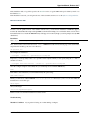
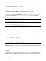
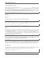
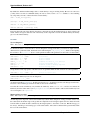
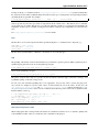
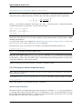
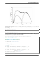
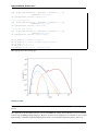
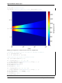
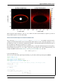
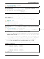
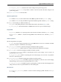
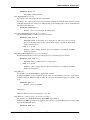
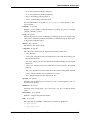
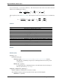
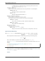
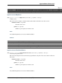
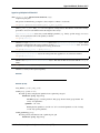
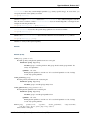
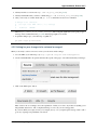
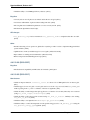
It is also possible to plot the dust properties:
d.plot('mydust.png')
which gives a plot that can be used to get an overview of all the dust properties:
3.3. Setting up models
17
Hyperion Manual, Release 0.9.7
Important note on units
In all of the following sections, quantities should be specified in the cgs system of units (e.g. 𝑐𝑚2 /𝑔 for the opacities).
Whether the opacities are specified per unit mass of dust or gas is not important, as long as the densities specified
when setting up the geometry are consistent. For example, if the opacities are specified per unit dust mass, the
densities specified when setting up the model should be dust densities.
18
Chapter 3. Documentation
Hyperion Manual, Release 0.9.7
Dust with isotropic scattering
Creating a dust object with isotropic scattering properties is very simple. First, import the IsotropicDust class:
from hyperion.dust import IsotropicDust
and create and instance of the class by specifying the frequency, albedo, and opacity to extinction (absorption +
scattering):
d = IsotropicDust(nu, albedo, chi)
where nu, albedo, and chi should be specified as lists or 1-d Numpy arrays, and nu should be monotonically
increasing. The albedo values should all be in the range 0 to 1, and the chi values should be positive. The
scattering matrix elements will be set to give isotropic scattering, and the emissivities and mean opacities will be set
assuming local thermodynamic equilibrium.
Dust with Henyey-Greenstein scattering
Creating a dust object with Henyey-Greenstein scattering properties is very similar to isotropic scattering, with the
exception that the scattering parameters have to be specified. The scattering is anisotropic, and the phase function is
defined by analytical functions (Henyey & Greenstein, 1941).
First, import the HenyeyGreensteinDust class:
from hyperion.dust import HenyeyGreensteinDust
and create an instance of the class by specifying the frequency, albedo, opacity to extinction (absorption + scattering),
and the anisotropy factor and the maximum polarization:
d = HenyeyGreensteinDust(nu, albedo, chi, g, p_lin_max)
where nu, albedo, chi, g and p_lin_max should be specified as lists or 1-d Numpy arrays, and nu should be
monotonically increasing. The albedo values should all be in the range 0 to 1, and the chi values should be positive.
The scattering matrix elements will be set to give the correct phase function for the scattering properties specified, and
the emissivities and mean opacities will be set assuming local thermodynamic equilibrium.
Fully customized 4-element dust
While the Henyey-Greenstein scattering phase function allows for anisotropic scattering, it approximates the phase
function by analytical equations. In some cases, it is desirable to instead use the full numerical phase function which
can be arbitrarily complex.
To set up a fully customized 4-element dust model, first import the SphericalDust class (this actually refers to
any kind of dust that would produce a 4-element scattering matrix, including randomly oriented non-spherical grains):
from hyperion.dust import SphericalDust
Then create an instance of this class:
d = SphericalDust()
Now that you have a dust ‘object’, you will need to set the optical properties of the dust, which include the albedo and
extinction coefficient (in cgs) as a function of frequency (in Hz):
d.optical_properties.nu = nu
d.optical_properties.albedo = albedo
d.optical_properties.chi = chi
3.3. Setting up models
19
Hyperion Manual, Release 0.9.7
where nu, albedo, and chi should be specified as lists or 1-d Numpy arrays, and nu should be monotonically
increasing. The albedo values should all be in the range 0 to 1, and the chi values should be positive.
Once these basic properties are set, you will need to set the scattering properties by setting the matrix elements. These
should be specified as a function of the cosine of the scattering angle, mu. The values of mu should be specified as a
1-d Numpy array:
d.optical_properties.mu = mu
Once nu and mu are set, the values of the scattering matrix elements can be set. These are stored in variables named
using the convention of Code & Whitney (1995): P1 (equivalent to S11), P2 (equivalent to S12), P3 (equivalent to
S44), and P4 (equivalent to -S34). Each of these variables should be specified as a 2-d array with dimensions (n_nu,
n_mu), where n_nu is the number of frequencies, and n_mu is the number of values of the cosine of the scattering
angle:
d.optical_properties.P1
d.optical_properties.P2
d.optical_properties.P3
d.optical_properties.P4
=
=
=
=
P1
P2
P3
P4
Alternatively, it is possible to call:
d.optical_properties.initialize_scattering_matrix()
After which P1, P2, P3, and P4 will be set to arrays with the right dimensions, and with all values set to zero. You
could for example set up an isotropic scattering matrix by setting the values of the arrays:
d.optical_properties.P1[:,
d.optical_properties.P2[:,
d.optical_properties.P3[:,
d.optical_properties.P4[:,
:]
:]
:]
:]
=
=
=
=
1.
0.
1.
0.
If nothing else is specified, the dust emissivity will be set assuming local thermodynamic equilibrium (i.e. it will be
set to the opacity to absorption times Planck functions).
Emissivities
By default, emissivities and mean opacities will be calculated under the assumption of local thermodynamic equilibrium for 1200 dust temperatures between 0.1 and 100000K, but this can be customized, as described below.
LTE emissivities To set the LTE emissivities manually, you can call the set_lte_emissivities method. For
example, to calculate the emissivities for 1000 temperatures between 0.1 and 2000K, you can do:
d.set_lte_emissivities(n_temp=1000,
temp_min=0.1,
temp_max=2000.)
The more temperatures the emissivities are calculated for, the more accurate the radiative transfer (Hyperion interpolates between emissivities, rather the picking the closest one) but the slower the dust file will be to generate and read
into Hyperion.
Custom emissivities If you want to specify fully customized emissivities as a function of specific energy, you can
instead do this by directly accessing the variables, which are stored as attributes to d.emissivities, i.e.:
20
Chapter 3. Documentation
Hyperion Manual, Release 0.9.7
d.emissivities.nu
d.emissivities.var
d.emissivities.jnu
d.emissivities.var_name
The attribute nu should be set to a 1-d array giving the frequencies that the emissivities are specified for, var should
be set to another 1-d array containing the values of the specific energy the emissivities are defined for, and jnu should
be set to a 2-d array with dimensions (len(nu), len(var)) giving the emissivities. In addition, you will need
to set var_name to ’specific_energy’ (in future, other kinds of emissivity variables may be supported). For
example, to set a constant emissivity as a function of frequency and specific energy, you can do:
d.emissivities.nu = np.logspace(8., 16., 100)
d.emissivities.var = np.logspace(-2., 8., 20)
# 100 values between 10^8 and 10^16
# 20 values of the specific energy
# between 10^-2 and 10^8
d.emissivities.jnu = np.ones(100, 20) # constant emissivities
d.emissivities.var_name = 'specific_energy'
Extrapolating optical properties
In some cases (see e.g. Common warnings) it can be necessary to extrapolate the dust properties to shorter and/or
longer wavelengths. While it would be preferable to do this extrapolation properly before passing the values to the
dust objects, in some cases the extrapolation is relatively straightforward, and you can make use of the following
extrapolation convenience functions:
d.optical_properties.extrapolate_wav(0.1, 1000)
d.optical_properties.extrapolate_nu(1.e5, 1.e15)
In the first case, the extrapolation is done by specifying wavelengths in microns, and in the second case by specifying
the frequency (in Hz).
The extrapolation is done in the following way:
• The opacity to extinction (chi) is extrapolated by fitting a power-law to the opacities at the two highest frequencies and following that power law, and similarly at the lowest frequencies. This ensures that the slope of
the opacity remains constant.
• The albedo is extrapolated by assuming that the albedo is constant outside the original range, and is set to the
same value as the values for the lowest and highest frequencies.
• The scattering matrix is extrapolated similarly to the albedo, by simply extending the values for the lowest and
highest frequencies to the new frequency range.
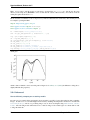
The plots shown higher up on this page have made use of these extrapolation methods.
Common warnings
One of the most common warnings when computing the LTE emissivities or writing out a dust file is the following:
WARNING: Planck function for lowest temperature not completely covered by opacity function
WARNING: Planck function for highest temperature not completely covered by opacity function
The LTE emissivity is set to 𝜅𝜈 𝐵𝜈 (𝑇 ), so you need to ensure that the opacity is defined over a frequency large enough
to allow this to be calculated from the lowest to the highest temperatures used for the LTE emissivities. The default
range is quite large (0.1 to 100000K) so you can either reduce this range (see LTE emissivities) or you should define
the optical properties over a larger frequency range (see Extrapolating optical properties for one way to do this).
3.3. Setting up models
21
Hyperion Manual, Release 0.9.7
More specifically, the frequency range should extend almost three orders of magnitude above the peak frequency for
the coldest temperature, and one order of magnitude below the peak frequency for the hottest temperature. For the
default temperature range for the LTE emissivities (0.1 to 100000K), this means going from about 5e7 to 5e16Hz (or
0.5nm to 5m) which is a huge frequency range, over which dust properties are often not known. However, in most
cases, a sensible extrapolation of the properties you have should be fine - the plots shown higher up on this page show
the values extrapolated to the required range. If you restrict yourself to a smaller temperature range (e.g. 3 to 1600K)
you can also reduce the required range significantly.
Note: If you do not fix this warning, the normalization of the emissivities will be off, and the results from the radiative
transfer may be incorrect!
Writing dust files without the Python library
If for any reason you wish to write the HDF5 dust files directly without using the Hyperion Python library, you can
find a detailed description of the format in Dust HDF5 Format.
Coordinate grids and physical quantities
In general, coordinate grids and density grids are set using methods of the form:
from hyperion.model import Model
m = Model()
m.set_<grid_type>_grid(...)
m.add_density_grid(density, dust)
where <grid_type> is the grid type being used, and dust is a dust file in HDF5 format specified either by filename,
or as a dust object. See Preparing dust properties for more details about creating and using dust files. For example, if
you are using a dust file named kmh.hdf5, you can specify this with:
m.add_density_grid(density, 'kmh.hdf5')
The add_density_grid method can be called multiple times if multiple density arrays are needed (for example if
different dust sizes have different spatial distributions).
Note: If you haven’t already done so, please make sure you read the Important Notes to understand whether to specify
dust or dust+gas densities!
Optionally, a specific energy distribution can also be specified in add_density_grid using the
specific_energy= argument:
m.add_density_grid(density, dust, specific_energy=specific_energy)
where specific_energy is given in the same format as density (see sections below). By default, the specific
energy specified is the initial specific energy used, and if the number of temperature iterations is not zero (see Specific
energy calculation) this specific energy gets replaced with the self-consistently calculated one in later iterations. If
instead you want this specific energy to be added to the self-consistently computed one after each iteration, see Initial
and additional specific energy.
Hyperion currently supports six types of 3-d grids:
• Cartesian grids
• Spherical polar grids
• Cylindrical polar grids
22
Chapter 3. Documentation
Hyperion Manual, Release 0.9.7
• AMR (Adaptive Mesh Refinement) grids
• Octree grids
• Voronoi grids
The following sections show how the different kinds of grids should be set up.
Regular 3-d grids
Geometry In the case of the cartesian and polar grids, you should define the wall position in each of the three directions, using cgs units for the spatial coordinates, and radians for the angular coordinates. These wall positions should
be stored in one 1-d NumPy array for each dimension, with one element more than the number of cells defined. The
walls can then be used to create a coordinate grid using methods of the form set_x_grid(walls_1, walls_2,
walls_3). The following examples demonstrate how to do this for the various grid types
• A 10x10x10 cartesian grid from -1pc to 1pc in each direction:
x = np.linspace(-pc, pc, 11)
y = np.linspace(-pc, pc, 11)
z = np.linspace(-pc, pc, 11)
m.set_cartesian_grid(x, y, z)
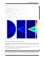
• A 2-d 400x200x1 spherical polar grid with radial grid cells logarithmically spaced between one solar radius and
100AU, and the first grid cell wall located at 0:
r = np.logspace(np.log10(rsun), np.log10(100 * au), 400)
r = np.hstack([0., r]) # add cell wall at r=0
theta = np.linspace(0., pi, 201)
phi = np.array([0., 2 * pi])
m.set_spherical_polar_grid(r, theta, phi)
• A 3-d 100x100x10 cylindrical polar grid with radial grid cells logarithmically spaced between one solar radius
and 100AU, and the first grid cell wall located at 0:
w = np.logspace(np.log10(rsun), np.log10(100 * au), 100)
w = np.hstack([0., w]) # add cell wall at w=0
z = np.linspace(-10 * au, 10 * au, 101)
phi = np.linspace(0, 2 * pi, 11)
m.set_cylindrical_polar_grid(w, z, phi)
Note: Spherical and cylindrical polar grids do not have to start at r=0 or w=0, but you need to make sure that all
sources are located inside the grid. For example, if you place a point source at the origin, you will need the first grid
cell wall to be at r=0 or w=0. In the above cases, since the grid cell walls are distributed logarithmically, the first grid
cell wall has to be added separately, hence the use of hstack, which is used to add a 0 at the start of the array.
Density and Specific Energy For regular cartesian and polar grids, a 3-d NumPy array containing the density array
is required, for example:
m.add_density_grid(np.ones((100,100,100)), 'kmh.hdf5')
for a 100x100x100 grid. Due to Numpy array conventions, the dimensions should be specified in reverse order, i.e.
(n_z, n_y, n_x) for a cartesian grid, (n_phi, n_theta, n_r) for a spherical polar grid, or (n_phi,
n_z, n_r) for a cylindrical polar grid.
Note that once you have set the grid geometry on a model, you can access variables that make it easy (if you wish) to
set up densities from analytical equations:
3.3. Setting up models
23
Hyperion Manual, Release 0.9.7
• m.grid.gx, m.grid.gy, and m.grid.gz for cartesian grids
• m.grid.gr, m.grid.gt, and m.grid.gp for spherical polar grids
• m.grid.gw, m.grid.gz, and m.grid.gp for cylindrical polar grids
These variables are the coordinates of the center of the cells, and each of these variables is a full 3-d array. For
example, m.grid.gx is the x position of the center of all the cells, and has the same shape as the density array needs
to have. In addition, the m.grid.shape variable contains the shape of the grid. This makes it easy to use analytical
prescriptions for the density. For example, to set up a sphere of dust with radius R in a cartesian grid, you could do:
density = np.zeros(m.grid.shape)
density[(m.grid.gx ** 2 + m.grid.gy ** 2 + m.grid.gz ** 2) < R ** 2] = 1.
This grid would have a density of 0 outside R, and 1 inside R. Note that of course you should probably be using a
spherical polar grid if you want to set up a sphere of dust, but the above example can be applied to more complicated
analytical dust structures.
AMR grids
Geometry AMR grids have to be constructed using the AMRGrid class:
from hyperion.grid import AMRGrid
amr = AMRGrid()
Levels can be added with:
level = amr.add_level()
And grids can be added to a level with:
grid = level.add_grid()
Grid objects have the following attributes which should be set:
• xmin - lower x position of the grid
• xmax - upper x position of the grid
• ymin - lower y position of the grid
• ymax - upper y position of the grid
• zmin - lower z position of the grid
• zmax - upper z position of the grid
• nx - number of cells in x direction
• ny - number of cells in y direction
• nz - number of cells in z direction
• quantities - a dictionary containing physical quantities (see below)
Once we have an AMR grid object, which we call amr here, the geometry can be set using:
m.set_amr_grid(amr)
The quantities attribute is unimportant for this step, as long as the geometry is correct.
For more details on how to create or read in an AMR object, and for a list of requirements and restrictions on the
geometry, see AMR Grids.
24
Chapter 3. Documentation
Hyperion Manual, Release 0.9.7
Note: If you load in your simulation data with the yt package, you can make use of the from_yt() method to easily
convert the simulation into a Hyperion AMRGrid object.
Density and Specific Energy Since AMR grids have a more complex structure than regular 3-d arrays, the density
should be added using an AMRGrid object. In this case, the quantity attribute should be set for each grid object.
For each physical quantity in the AMR grid, the dictionary should have an entry of the form:
grid.quantities[<quantity>] = quantity_array
where <quantity> is a string containing the name of the quantity (e.g. density) and quantity_array should
be a Numpy array with dimensions (grid.nz, grid.ny, grid.nx) (see AMR Grids for more details).
When calling add_density_grid, the density should be specified as an item of the AMRGrid object:
m.add_density_grid(amr_object['density'], dust_file)
for example:
m.add_density_grid(amr['density'], 'kmh.hdf5')
Specific energies can be specified using the same kinds of objects and using the specific_energy argument:
m.add_density_grid(amr['density], dust_file,
specific_energy=amr['specific_energy'])
Note that in this example, the amr object contains the geometry, the density, and the specific energy (i.e. it is not
necessary to create a separate AMRGrid object for each one).
Octree grids
Geometry An Octree is a hierarchical grid format where each cell can be divided into eight children cells. At the
top level is a single cell that covers the whole spatial domain being considered. To set up an Octree, the following
information is needed:
• x, y, z - the coordinates of the center of the parent cell
• dx, dy, dz - the size of the parent cell
• refined a 1-d sequence of booleans giving the structure of the grid.
The refined sequence contains all the information regarding the hierarchy of the grid, and is described in Octree
Grids. Once this sequence is set, the geometry can be set with:
m.set_octree_grid(x, y, z, dx, dy, dz, refined)
Density and Specific Energy Densities (and optionally specific energies) should be specified in the same manner as
the regular grids, but should be specified as a 1-d Numpy array with the same length as the refined list, where each
density value corresponds to the equivalent cell in the refined list. Density values for cells with refined set to
True will be ignored, and can be set to zero.
Voronoi grids
Geometry A Voronoi grid is based on the concept of 3D Voronoi diagrams. A Voronoi grid is created from a set
of user-specified seed points. Each seed point corresponds to a single grid cell, and the cell in which a seed point is
located is defined geometrically by the set of all points closer to that seed than to any other.
3.3. Setting up models
25
Hyperion Manual, Release 0.9.7
Voronoi cells are always guaranteed to be convex polyhedra. The number and distribution of the seed points are
arbitrary (clearly, for best results the values of these two parameters should be chosen following some physical intuition
or with a specific goal in mind - e.g., seed points could be more numerous where higher resolution is needed).
In order to set up a Voronoi grid, the following information is needed:
• x, y, z - three 1-d Numpy arrays of equal size representing the coordinates of the seed points. The size of these
arrays implicitly defines the number of seed points.
The geometry can be set with:
m.set_voronoi_grid(x, y, z)
Density and Specific Energy Densities (and optionally specific energies) should be specified in the same manner
as the regular grids, but should be specified as a 1-d Numpy array with the same length as the number of seed points.
Each density value in the array refers to the cell containing the corresponding seed point.
Luminosity sources
General notes
Sources can be added to the model using methods of the form m.add_*_source(). For example adding a point
source can be done with:
source = m.add_point_source()
These methods return a source ‘object’ that can be used to set and modify the source parameters:
source = m.add_point_source()
source.luminosity = lsun
source.temperature = 10000.
source.position = (0., 0., 0.)
Note: It is also possible to specify the parameters using keyword arguments during initialization, e.g.:
m.add_point_source(luminosity=lsun, temperature=10000.,
position=(0., 0., 0.))
though this can be longer to read for sources with many arguments.
All sources require a luminosity, given by the luminosity attribute (or luminosity= argument), and the emission
spectrum can be defined in one of three ways:
• by specifying a spectrum using the spectrum attribute (or spectrum= argument). The spectrum should
either be a (nu, fnu) pair or an instance of an atpy.Table with two columns named ’nu’ and ’fnu’.
For example, given a file spectrum.txt with two columns listing frequency and flux, the spectrum can be
set using:
import numpy
spectrum = np.loadtxt('spectrum.txt', dtype=[('nu', float),
('fnu', float)])
source.spectrum = (spectrum['nu'], spectrum['fnu'])
• by specifying a blackbody temperature using the temperature attribute (or temperature= argument).
This should be a floating point value.
• by using the local dust emissivity if neither a spectrum or temperature are specified.
26
Chapter 3. Documentation
Hyperion Manual, Release 0.9.7
Note: By default, the number of photons emitted is proportional to the luminosity, so in cases where several sources
with very different luminosities are included in the models, some sources might be under-sampled. You can instead
change the configuration to emit equal number of photons from all sources - see Multiple sources for more details.
Point sources
A point source is defined by a luminosity, a 3-d cartesian position (set to the origin by default), and a spectrum or
temperature. The following examples demonstrate adding different point sources:
• Set up a 1 solar luminosity 10,000K point source at the origin:
source = m.add_point_source()
source.luminosity = lsun # [ergs/s]
source.temperature = 10000. # [K]
• Set up two 0.1 solar luminosity 1,300K point sources at +/- 1 AU in the x direction:
# Set up the first source
source1 = m.add_point_source()
source1.luminosity = 0.1 * lsun # [ergs/s]
source1.position = (au, 0, 0) # [cm]
source1.temperature = 1300. # [K]
# Set up the second source
source2 = m.add_point_source()
source2.luminosity = 0.1 * lsun # [ergs/s]
source2.position = (-au, 0, 0) # [cm]
source2.temperature = 1300. # [K]
• Set up a 10 solar luminosity source at the origin with a spectrum read in from a file with two columns giving
wavelength (in microns) and monochromatic flux:
# Use NumPy to read in the spectrum
import numpy as np
data = np.loadtxt('spectrum.txt', dtype=[('wav', float), ('fnu', float)])
# Convert to nu, fnu
nu = c / (data['wav'] * 1.e-4)
fnu = data['fnu']
# Set up the source
source = m.add_point_source()
source.luminosity = 10 * lsun
source.spectrum = (nu, fnu)
# [ergs/s]
Note: Regardless of the grid type, the coordinates for the sources should always be specified in cartesian coordinates,
and in the order (x, y, z).
If you want to set up many point sources (for example for a galaxy model) you may instead want to consider using a
Point source collections.
Spherical sources
Adding spherical sources is very similar to adding point sources, with the exception that a radius can be specified:
3.3. Setting up models
27
Hyperion Manual, Release 0.9.7
source = m.add_spherical_source()
source.luminosity = lsun # [ergs/s]
source.radius = rsun # [cm]
source.temperature = 10000. # [K]
It is possible to add limb darkening, using:
source.limb = True
Spots on spherical sources
Adding spots to a spherical source is straightforward. Spots behave the same as other sources, requiring a luminosity,
spectrum, and additional geometrical parameters:
source = m.add_spherical_source()
source.luminosity = lsun # [ergs/s]
source.radius = rsun # [cm]
source.temperature = 10000. # [K]
spot = source.add_spot()
spot.luminosity = 0.1 * lsun # [ergs/s]
spot.longitude = 45. # [degrees]
spot.latitude = 30. # [degrees]
spot.radius = 5. # [degrees]
spot.temperature = 20000. # [K]
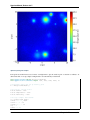
Diffuse sources
Diffuse sources are defined by a total luminosity, and a probability distribution map for the emission, defined on the
same grid as the density. For example, if the grid is defined on a 10x10x10 grid, the following will add a source which
emits photons from all cells equally:
source = m.add_map_source()
source.luminosity = lsun # [ergs/s]
source.map = np.ones((10, 10, 10))
By default, if no spectrum or temperature is provided, photons will be emitted using the local emissivity of the dust.
However, you can also specify either a temperature or a spectrum as for Point Sources and Spherical Sources, e.g:
source.temperature = 10000.
# [K]
or:
source.spectrum = (nu, fnu)
Note: The map array does not need to be normalized.
External sources
There are two kinds of external illumination sources, spherical and box sources - the former being more suited to
spherical polar grids, and the latter to cartesian, AMR, and octree grids (there is no cylindrical external source for
cylindrical grids at this time). In both cases, photons are emitted inwards isotropically. For example, an external
spherical source can be added with:
28
Chapter 3. Documentation
Hyperion Manual, Release 0.9.7
source = m.add_external_spherical_source()
source.luminosity = lsun # [ergs/s]
source.radius = pc # [cm]
source.temperature = 10000. # [K]
As for point and spherical sources, the position of the center can also be set, and defaults to the origin. External box
sources have a bounds attribute instead of radius and position:
source = m.add_external_box_source()
source.luminosity = lsun # [ergs/s]
source.bounds = [[-pc, pc], [-pc, pc], [-pc, pc]]
source.temperature = 10000. # [K]
# [cm]
where the bounds attribute is given as [[xmin, xmax], [ymin, ymax], [zmin, zmax]].
See How to set the luminosity for an external radiation field for information on setting the luminosity correctly in order
to reproduce a given intensity field.
Note: Even though these sources are referred to as ‘external’, they have to be placed inside the outermost walls of the
grid. The sources are not box-shared source or spherical source that can be placed outside the grid, but rather sources
that emit inwards instead of outwards, making it possible to simulate an external radiation field.
Plane parallel sources
Finally, it is possible to add circular plane parallel sources (essentially a circular beam with a given origin and direction):
source = m.add_plane_parallel_source()
source.luminosity = lsun # [ergs/s]
source.radius = rsun # [cm]
source.temperature = 10000. # [K]
source.position = (au, 0., 0.) # [cm]
source.direction = (45., 0.) # [degrees]
where direction is a tuple of (theta, phi) that gives the direction of the beam.
Point source collections
In cases where you want to set up more than a few dozen point sources, it may be worth instead using a point
source collection, which can contain an arbitrary number of point sources with different luminosities, and a common
temperature or spectrum. To add a point source collection, use e.g.:
source = m.add_point_source_collection()
The attributes are the same as for the Point Sources but the source.luminosity attribute should be set to an
array with as many elements as sources, and the source.position attribute should be set to a 2-d array where
the first dimension matches source.luminosity, and with 3 elements in the second dimension (x, y, and z). The
following example shows how to set up 1000 random point sources with random positions from -1au to 1au in all
directions, and with random luminosities between 0 and lsun:
N
x
y
z
=
=
=
=
1000
np.random.uniform(-1., 1, N) * au
np.random.uniform(-1., 1, N) * au
np.random.uniform(-1., 1, N) * au
3.3. Setting up models
29
Hyperion Manual, Release 0.9.7
source = m.add_point_source_collection()
source.luminosity = np.random.random(N) * lsun
source.position = np.vstack([x, y, z]).transpose()
source.temperature = 6000.
In terms of photon sampling, a point source collection acts as a single source with a luminosity given by the sum of
the components - so if you have one point source collection and one spherical source with the same total luminosity,
the number of photons will be evenly split between the two. Within the point source collection, the number of photons
is split according to luminosity.
Setting up images and SEDs
There are two main kinds of images/SEDs that can be produced for each model: images/SEDs computed by binning
the photons as they escape from the density grid, and images/SEDs computed by peeling off photon packets at each
interaction into well defined directions. The latter provide more accurate SEDs and much better signal-to-noise, and
are likely to be more commonly used than the former.
The code currently allows at most one set of binned images, and any number of sets of peeled images. A set is defined
by a wavelength range, image resolution and extent, and any number of viewing angles.
Creating a set of images
To add a set of binned images/SEDs to the model, use:
image = m.add_binned_images()
and to create a set of peeled images/SEDs to the model, use:
image = m.add_peeled_images()
Only one set of binned images can be added, but any number of sets of peeled image can be added. In general, peeled
images are recommended because binned images suffer from low signal-to-noise, and angle averaging of images.
The wavelength range (in microns) for the images/SEDs should be specified using:
image.set_wavelength_range(n_wav, wav_min, wav_max)
The image size in pixels and the extent of the images should be specified using:
image.set_image_size(n_x, n_y)
image.set_image_limits(xmin, xmax, ymin, ymax)
where the image limits should be given in cm. The apertures for the SEDs can be specified using:
image.set_aperture_radii(n_ap, ap_min, ap_max)
where the radii should be given in cm. If this is not specified, the default is to have one aperture with infinite size, i.e.
measuring all the flux.
For binned images, the number of bins in the theta and phi direction should be specified using:
image.set_viewing_bins(10, 10)
whereas for peeled images, the viewing angles should be specified as lists or arrays of theta and phi values, in degrees.
For example, the following produces images from pole-on to edge-on at constant phi using 20 viewing angles:
30
Chapter 3. Documentation
Hyperion Manual, Release 0.9.7
# Set number of viewing angles
n_view = 20
# Generate the viewing angles
theta = np.linspace(0., 90., n_view)
phi = np.repeat(45., n_view)
# Set the viewing angles
image.set_viewing_angles(theta, phi)
Note: For peeled images, the number of viewing angles directly impacts the performance of the code - once the
specific energy/temperature has been computed, the code will then run approximately in a time proportional to the
number of viewing angles.
Uncertainties
Uncertainties can be computed for SEDs/images (doubling the memory/disk space required):
image.set_uncertainties(True)
Stokes components
By default, to save memory and disk space, the Stokes components other than I for the images are not saved. To enable
the storage of the Stokes components other than I, make use of the set_stokes method:
sed.set_stokes(True)
or:
image.set_stokes(True)
If you do not do this, then you will not be able to make use of the stokes= option in get_sed() and
get_image().
Note: In Hyperion 0.9.3 and earlier versions, this option did not exist and Stokes components were all saved by
default. Note that the default behavior is now changed. However, files produced in Hyperion 0.9.3 and earlier will
behave as if the option was set to True for backward-compatibility.
File output
Finally, to save space, images can be written out as 32-bit floats instead of 64-bit floats. To write them out as 32-bit
floats, use:
image.set_output_bytes(4)
and to write them out as 64-bit floats, use:
image.set_output_bytes(8)
3.3. Setting up models
31
Hyperion Manual, Release 0.9.7
Tracking photon origin
SEDs/images can also be split into emitted/thermal or scattered components from sources or dust (4 combinations).
To activate this, use:
image.set_track_origin('basic')
It is also possible to split the SED into individual sources and dust types:
image.set_track_origin('detailed')
For example, if five sources and two dust types are present, there will be 14 components in total: five for photons
emitted from sources, two for photons emitted from dust, five for photons emitted from sources and subsequently
scattered, and two for photons emitted from dust and subsequently scattered.
Finally, it is also possible to split the photons as a function of how many times they scattered:
image.set_track_origin('scatterings', n_scat=5)
where n_scat gives the maxmimum number of scatterings to record.
See Post-processing models for information on how to extract this information from the output files.
Note: If you are using the AnalyticalYSOModel class and are interested in separating the disk, envelope, and
other components, but are using the same dust file for the different components, these will by default be merged prior
to the radiative transfer calculation, so you will need to set merge_if_possible=False when calling write()
to prevent this (see write() for more information).
Disabling SEDs or Images
When adding a set of binned or peeled images, it is possible to disable the SED or image part:
image = m.add_binned_images() # Images and SEDs
image = m.add_binned_images(image=False) # SEDs
image = m.add_binned_images(sed=False) # Images
image = m.add_peeled_images() # Images and SEDs
image = m.add_peeled_images(image=False) # SEDs
image = m.add_peeled_images(sed=False) # Images
Advanced
A few more advanced parameters are available for peeled images, and these are described in Advanced settings for
peeled images.
Example
The following example creates two sets of peeled SEDs/images. The first is used to produce an SED with 250 wavelengths from 0.01 to 5000. microns with uncertainties, and the second is used to produce images at 5 wavelengths
between 10 and 100 microns, with image size 100x100 and extending +/-1pc in each direction:
image1 = m.add_peeled_images(image=False)
image1.set_wavelength_range(250, 0.01, 5000.)
image1.set_uncertainties(True)
32
Chapter 3. Documentation
Hyperion Manual, Release 0.9.7
image2 = m.add_peeled_images(sed=False)
image2.set_wavelength_range(5, 10., 100.)
image2.set_image_size(100, 100)
image2.set_image_limits(-pc, +pc, -pc, +pc)
Radiative transfer settings
Once the coordinate grid, density structure, dust properties, and luminosity sources are set up, all that remains is to
set the parameters for the radiation transfer algorithm, including number of photons to use, or whether to use various
optimization schemes.
Number of photons
The number of photons to run in various iterations is set using the following method:
m.set_n_photons(initial=1000000, imaging=1000000)
where initial is the number of photons to use in the iterations for the specific energy (and therefore temperature),
and imaging is the number of photons for the SED/image calculation, whether using binned images/SEDs or peelingoff.
In addition, the stats= argument can be optionally specified to indicate how often to print out performance statistics
(if it is not specified a sensible default is chosen).
Since the number of photons is crucial to produce good quality results, you can read up more about setting sensible
values at Choosing the number of photons wisely.
Specific energy calculation
To set the number of initial iterations used to compute the dust specific energy, use e.g.:
m.set_n_initial_iterations(5)
Note that this can also be zero, in which case the temperature is not solved, and the radiative transfer calculation
proceeds to the image/SED calculation (this is useful for example if one is making images at wavelengths where
thermal emission is negligible, or if a specific energy/temperature was specified as input).
It is also possible to tell the radiative transfer algorithm to exit these iterations early if the specific energy has converged.
To do this, use:
m.set_convergence(True, percentile=100., absolute=0., relative=0.)
where the boolean value indicates whether to use convergence detection (False by default), and percentile,
absolute, and relative arguments are explained in more detail in Section 2.4 of Robitaille (2011). For the
benchmark problems of that paper, the values were set to:
m.set_convergence(True, percentile=99., absolute=2., relative=1.02)
which are reasonable starting values. Note that if you want to use convergence detection, you should make sure that the
value for set_n_initial_iterations is not too small, otherwise the calculation might stop before converging.
When running the main Hyperion code, convergence statistics are printed out, and it is made clear when the specific
energy has converged.
3.3. Setting up models
33
Hyperion Manual, Release 0.9.7
Initial and additional specific energy
Another option that is related to the specific energy is set_specific_energy_type(). This is used to control
how any specific energy passed to add_density_grid() is used. By default, the specific energy specified is the
initial specific energy used, and if the number of temperature iterations is not zero (see Specific energy calculation)
this specific energy gets replaced with the self-consistently calculated one in later iterations. If instead you want this
specific energy to be added to the self-consistently computed one after each iteration, you can set:
m.set_specific_energy_type('additional')
This can be used for example if you need to take into account an additional source of heating that cannot be modelled
by Hyperion.
Raytracing
To enable raytracing (for source and dust emission, but not scattering), simply use:
m.set_raytracing(True)
This algorithm is described in Section 2.6.3 of Robitaille (2011). If raytracing is used, you will need to add the
raytracing_sources and raytracing_dust arguments to the call to set_n_photons, i.e.:
m.set_n_photons(initial=1000000, imaging=1000000,
raytracing_sources=1000000, raytracing_dust=1000000)
Diffusion
If the model density contains regions of very high density where photons get trapped or do not enter, one can enable
the modified random walk (MRW; Min et al. 2009, Robitaille 2010) in order to group many photon interactions into
one. The MRW requires a parameter gamma which is used to determine when to start using the MRW (see Min et
al. 2009 for more details). By default, this parameter is set to 1. The following example shows how to enable the
modified random walk, and set the gamma parameter to 2:
m.set_mrw(True, gamma=2.)
In some cases (such as protoplanetary disks) very optically thick regions do not receive any radiation. In cases where
the temperature in these regions is important, one can use the partial diffusion approximation (PDA; Min et al. 2009)
to solve the diffusion equation over the grid and find the missing temperatures:
m.set_pda(True)
Note however that if more than 10,000 cells have low photon counts and require the PDA, this can be very slow, so
this option is only recommended in cases where you know it is absolutely needed. In most cases, if photons cannot
reach inside certain cells, these cells are unlikely to be contributing a significant amount of flux to SEDs or images.
Dust sublimation
To set whether and how to sublimate dust, first the dust file needs to be read in (or initialized in the script), the
sublimation parameters should be set, and the dust object should be passed directly to add_density:
from hyperion.dust import SphericalDust
d = SphericalDust('kmh.hdf5')
d.set_sublimation_temperature('fast', temperature=1600.)
34
Chapter 3. Documentation
Hyperion Manual, Release 0.9.7
m.add_density_grid(density, d)
The first argument of set_sublimation_temperature can be none (dust sublimation does not occur), cap
(temperatures in excess of the one specified will be reset to the one given), slow (dust with temperatures in excess of
the one specified will be gradually destroyed), or fast (dust with temperatures in excess of the one specified will be
immediately destroyed). For more information, see Section 2.7.3 of Robitaille (2011).
Multiple sources
By default, the number of photons emitted is proportional to the luminosity of the sources, so in cases where several
sources with very different luminosities are included in the models, some sources might be under-sampled. In some
cases, this will not be a problem, but in some cases you may want to emit equal numbers of photons from each source
instead. For example, if you have two sources that have a bolometric luminosity that is different by a factor of 100, but
at the specific wavelength you are interested in they have the same flux, then you will probably want equal numbers of
photons for both sources. You can enable this with:
m.set_sample_sources_evenly(True)
Note that this does not yet cause point sources within Point source collections to be evenly sampled. For the purposes
of this option, a point source collection counts as a single source.
Outputting physical quantities
It is possible to write out a number of physical arrays for each iteration, or just the last iteration. To do this, you will
need to set the parameters in Models.conf.output:
# Density
m.conf.output.output_density = 'last'
# Density difference (shows where dust was destroyed)
m.conf.output.output_density_diff = 'none'
# Energy absorbed (using pathlengths)
m.conf.output.output_specific_energy = 'last'
# Number of unique photons that passed through the cell
m.conf.output.output_n_photons = 'last'
Each value can be set to all (output all iterations), last (output only after last iteration), or none (do not output).
The default is to output only the last iteration of specific_energy. To find out how to view these values, see
Post-processing models
Advanced parameters
There are a number of more advanced parameters to control the radiative transfer, but since they are not essential
initially, they are described in the Advanced configuration section.
Once the model is set up, you can write it out to the disk for use with the Fortran radiation transfer code:
m.write('example.rtin')
See write() for information about the available options.
3.3. Setting up models
35
Hyperion Manual, Release 0.9.7
3.3.2 Analytical YSO Models
The Arbitrary Models class should allow users to set up arbitrary problems. However, the Python module also provides
classes that build on top of Model that make it easy to specify certain kinds of problems. These classes support all
the methods available for the Model class, and define new ones. The AnalyticalYSOModel makes it easy to set
up sources with flared disks, and rotationally flattened envelopes, optionally with bipolar cavities. To use this class,
you will first need to import it:
from hyperion.model import AnalyticalYSOModel
it is then easy to set up such a model using:
m = AnalyticalYSOModel()
The model can then be set up using methods of the AnalyticalYSOModel instance. This is described in more
detail in the following section:
Setting up a YSO model
Note: If you haven’t already done so, please make sure you read the Important Notes to understand whether to specify
dust or dust+gas densities!
Source parameters
The stellar luminosity and radius should be set via the following attributes:
m.star.luminosity = 5 * lsun
m.star.radius = 2 * rsun
and either the temperature or the spectrum of the source can be set, using:
m.star.temperature = 10000.
or:
m.star.spectrum = (nu, fnu)
Flared disks
Flared disks can be added using the add_flared_disk() method, and capturing the reference to the
FlaredDisk object to set the parameters further:
disk = m.add_flared_disk()
disk.mass = 0.01 * msun
disk.rmin = 10 * rsun
disk.rmax = 300 * au
disk.r_0 = 100. * au
disk.h_0 = 5 * au
disk.p = -1
disk.beta = 1.25
36
#
#
#
#
#
#
#
Disk mass
Inner radius
Outer radius
Radius at which h_0 is defined
Disk scaleheight at r_0
Radial surface density exponent
Disk flaring power
Chapter 3. Documentation
Hyperion Manual, Release 0.9.7
Envelopes
Power-law spherically symmetric envelope The simplest kind of envelope is a spherically symmetric envelope with
a power-law distribution in density. A power-law envelope can be added using the add_power_law_envelope()
method, and capturing the reference to the PowerLawEnvelope object to set the parameters further:
envelope = m.add_power_law_envelope()
envelope.mass = 0.1 * msun
#
envelope.rmin = au
#
envelope.rmax = 10000 * au
#
envelope.power = -2
#
Envelope mass
Inner radius
Outer radius
Radial power
Ulrich rotationally flattened envelope A more complex envelope density distribution is that of Ulrich
(1976), which consists of a rotationally flattened envelope. A power-law envelope can be added using the
add_ulrich_envelope() method, and capturing the reference to the UlrichEnvelope object to set the parameters further:
envelope = m.add_ulrich_envelope()
envelope.mdot = 1e-4 * msun / yr
envelope.rmin = 0.1 * au
envelope.rc = 100 * au
envelope.rmax = 1000 * au
#
#
#
#
Infall rate
Inner radius
Centrifugal radius
Outer radius
As mentioned in the Important Notes, the infall rate mdot is not necessarily the dust+gas infall rate - for instance if
the dust opacities are per unit dust mass, the infall rate specified should only include the dust (because it is only used
to set the density structure, and does not add any accretion luminosity).
Note: the Ulrich (1976) solution is sometimes (incorrectly) referred to as the Terebey, Shu, and Cassen (TSC)
solution, which is much more complex. The Ulrich envelope implemented here is the same envelope type as is often
implemented in other radiation transfer codes.
Bipolar cavities
Once an envelope has been created, bipolar cavities can be carved out in it by calling the add_bipolar_cavities
method on the envelope object, which returns a BipolarCavity instance:
cavity = envelope.add_bipolar_cavities()
cavity.power = 1.5
# Shape exponent z~w^exp
cavity.r_0 = 1.e-20
# Radius to specify rho_0 and theta_0
cavity.theta_0 = 10
# Opening angle at r_0 (degrees)
cavity.rho_0 = 1.e-20
# Density at r_0 in g/cm^3
cavity.rho_exp = 0.
# Vertical density exponent
Ambient medium
In addition to disks and envelopes, it is also possible to add a constant ambient density medium using the
add_ambient_medium() method, which returns an AmbientMedium instance:
ambient = m.add_ambient_medium()
ambient.rmin = 0.1 * au
ambient.rmax = 1000 * au
ambient.rho = 1.e-20
3.3. Setting up models
# Inner radius
# Outer radius
# Ambient density in g/cm^3
37
Hyperion Manual, Release 0.9.7
By default, the ambient medium simply adds a constant density to any pre-existing density. However, in some cases
you may want to use this as a minimum density. In order to do this, set the subtract attribute to a list containing
any component you want to subtract from the constant density:
disk = m.add_flared_disk()
...
envelope = m.add_ulrich_envelope()
...
ambient = m.add_ambient_medium()
...
ambient.subtract = [envelope, disk]
In regions where the sum of the densities from these components exceeds the ambient density, no dust is added to the
model, whereas in regions where the sum of the density of the components is below the ambient density, the density
gets set to the ambient density.
Accretion
Viscous dissipation
Note: This feature is still experimental, please use with caution and report any issues!
To simulate the effects of accretion due to viscous dissipation of energy in the disk, you can use an ‘alpha accretion’
disk instead of a plain flared disk. Such disks can be added using the add_alpha_disk() method, and capturing
the reference to the AlphaDisk object to set the parameters further. The parameters are the same as for flared disks:
disk = m.add_alpha_disk()
disk.mass = 0.01 * msun
disk.rmin = 10 * rsun
disk.rmax = 300 * au
disk.r_0 = 100. * au
disk.h_0 = 5 * au
disk.p = -1
disk.beta = 1.25
#
#
#
#
#
#
#
Disk mass
Inner radius
Outer radius
Radius at which h_0 is defined
Disk scaleheight at r_0
Radial surface density exponent
Disk flaring power
except that the accretion properties of the disk can also be specified. Either the disk accretion rate can be specified:
disk.mdot = 1e-6 * msun / yr
# Disk accretion rate
or the accretion luminosity from viscous dissipation:
disk.lvisc = 0.01 * lsun
As mentioned in the Important Notes, the disk accretion rate mdot should always be the total dust+gas accretion rate,
because it is the total dust+gas accretion rate that sets the accretion luminosity.
Note that this accretion luminosity only includes the luminosity down to disk.rmin, and does not include the
luminosity from the stellar surface (see Magnetospheric accretion). For more details on the accretion luminosity from
viscous dissipation, see AlphaDisk.
Magnetospheric accretion
Note: This feature is still experimental, please use with caution and report any issues!
Another important component of the accretion luminosity is that from the dissipation of energy as matter accretes onto
the central star from the inner edge of the gas disk. In a simplistic model of magnetospheric accretion, matter free-falls
from the radius at which the disk is truncated by the magnetosphere to the surface of the star. Half the energy goes
into X-rays, and half goes into heating spots on the stellar surface, and is then re-emitted with a spectrum hotter than
the rest of the stellar surface.
38
Chapter 3. Documentation
Hyperion Manual, Release 0.9.7
To help set this up, a convenience method setup_magnetospheric_accretion() is provided, which takes
the accretion rate, the radius at which the matter free-falls from, the spot covering fraction, and optionally parameters
describing the X-ray spectrum. For example:
m.setup_magnetospheric_accretion(1.e-6 * msun / yr, 5 * m.star.radius, 0.2)
will set up an X-ray and a hot spot emission component from the central source. The method does not currently
set up actual spots, it assumes that the spots cover the star uniformly, and the spot covering fraction determines the
temperature of the hot spots (a smaller covering fraction results in a larger hot spot temperature for a fixed accretion
rate).
See setup_magnetospheric_accretion() for more details.
Dust
The dust file to use for each component should be specified using the dust attribute for the component, e.g.:
disk.dust = 'www003.hdf5'
envelope.dust = 'kmh.hdf5'
cavity.dust = 'kmh_hdf5'
The dust can be specified either as a filename or an instance of one of the dust types.
Grid
The gridding of the density can done automatically, but you will need to specify a grid size. Either a spherical polar or
cylindrical polar grid can be used. To use the spherical polar grid:
m.set_spherical_polar_grid_auto(n_r, n_theta, n_phi)
and to use the cylindrical polar grid:
m.set_cylindrical_polar_grid_auto(n_w, n_z, n_phi)
The grid is set up in such a way as to provide very fine resolution at the inner edge of the disk or envelope, and
logarithmic spacing of cell walls on large scales.
In some cases, this automated gridding may not be appropriate, and you may want to specify the grid geometry yourself, for example if you have other sources of emission than the one in the center. In this case, the
set_spherical_polar_grid() and set_cylindrical_polar_grid() methods described in Coordinate grids and physical quantities can be used. As a reminder, these take the position of the walls as arguments rather
than the number of cells, e.g.:
r = np.logspace(np.log10(rsun), np.log10(100 * au), 400)
r = np.hstack([0., r]) # add cell wall at r=0
theta = np.linspace(0., pi, 201)
phi = np.array([0., 2 * pi])
m.set_spherical_polar_grid(r, theta, phi)
Optically thin temperature radius
When setting up the disk or envelope inner/outer radii, it can sometimes be useful to set it to a ‘dynamic’ quantity such
as the sublimation radius of dust. A convenience class is available for this purpose:
3.3. Setting up models
39
Hyperion Manual, Release 0.9.7
from hyperion.util.convenience import OptThinRadius
The OptThinRadius class allows you to simply specify a temperature 𝑇𝑑 , and when preparing the model, the code
will pick the radius at which the temperature would be equal to the value specified if the dust was optically thin:
[︂
]︂2 }︃−1/2
𝑇𝑑4 𝜅plank (𝑇𝑑 )
1− 1−2 4
𝑇eff
𝜅⋆
{︃
𝑟 = 𝑟⋆
where 𝑇eff,⋆ is the effective temperature of the central source, and 𝜅⋆) is the mean opacity to a radiation field with the
spectrum of the central source. In practice, you can use this as follows:
disk = m.add_flared_disk()
disk.mass = 0.01 * msun
disk.rmin = OptThinRadius(1600.)
disk.rmax = 300. * au
...
and the inner disk radius will be set to the radius at which the optically thin temperature would have fallen to 1600K,
emulating dust sublimation.
To set up the dust, images, and configuration, see the Preparing dust properties, Setting up images and SEDs, and
Radiative transfer settings sections of the Arbitrary Models description.
Once the model is set up, you can write it out to the disk for use with the Fortran radiation transfer code:
m.write('example.rtin')
See write() for information about the available options.
Note: One of the available options is merge_if_possible=, which if set to True will merge the various density
components into a single one if the dust types match. This allows the code to run faster, but on the other hand means
that if tracking e.g. photon origin, the separate origin of components that have been merged will be lost. This option
is enabled by default, but you may want to disable it.
And the following pages give details and advice on particular configuration settings:
3.3.3 Choosing the number of photons wisely
Note: This section is incomplete at this time, and only covers choosing the photon numbers for the specific energy/temperature calculation.
As described in Radiative transfer settings and Advanced configuration, the number of photons should be set with the:
m.set_n_photons(...)
method. The arguments to specify depend on the type of calculation
Specific Energy/Temperature
The number of photons used in the initial specific energy calculation is set with the initial= keyword argument. A
good starting value for this if the density grid is close to optically thin is to set it to be at least the number of cells in
the grid. If the optical depth is much larger, e.g. in the case of protoplanetary disks, one may need to choose 10 or 100
times the number of cells in order to get a good signal-to-noise.
40
Chapter 3. Documentation
Hyperion Manual, Release 0.9.7
The best way to check whether an adequate value has been chosen is to extract the specific energy or temperature grids
as described in Extracting physical quantities, and to visualize these. The following image shows an example of the
specific energy in an azimuthally symmetric cylindrical grid (i.e. showing z vs r) where the initial number of photons
is too low. Individual photon propagation paths can be seen, and the temperature map is very poorly defined.
If the temperature is increased, then the temperature map becomes smoother, though in the densest regions, the temperature is still very noisy:
3.3. Setting up models
41
Hyperion Manual, Release 0.9.7
Once it is not possible to realistically increase the number of photons without running into computational limitations,
one can instead resort to using the PDA approximation (described in Diffusion) to compute the missing temperature
values in the most optically thick regions.
Note: it is possible to write model input files yourself directly in HDF5 and bypass the Python library entirely (but
42
Chapter 3. Documentation
Hyperion Manual, Release 0.9.7
this is reserved for advanced users!). See Model Input HDF5 Format for more information.
3.4 Running models
3.4.1 Using the hyperion command-line wrapper
Once an .rtin file has been created (see Setting up models), the model can be run using the compiled Fortran code.
Note that the model can be run on a different computer/cluster to the computer on which is was set up, because the
.rtin files are portable.
The easiest way to run a model is to invoke the hyperion command-line utility, specifying the input and output file
(we use the .rtout extensions for output files):
hyperion model.rtin model.rtout
Note: hyperion is a command-line Python wrapper around the Fortran binaries that gets installed with the Python
Hyperion library.
To run Hyperion in parallel, you can use:
hyperion -m <n_processes> model.rtin model.rtout
where <n_processes> is the number of processes to run in parallel (does not need to equal the number of cores in
the computer or cluster). For example, to run the code over 24 processes, you can use:
hyperion -m 24 model.rtin model.rtout
This may not work with all MPI installations. If you have issues, see the next section on calling the Fortran binaries
directly (and report the issue).
3.4.2 Calling the Fortran binaries directly
hyperion is in fact a wrapper to grid specific binaries:
• hyperion_car and hyperion_car_mpi for cartesian grids
• hyperion_cyl and hyperion_cyl_mpi for cylindrical polar grids
• hyperion_sph and hyperion_sph_mpi for spherical polar grids
• hyperion_amr and hyperion_amr_mpi for AMR grids
• hyperion_oct and hyperion_oct_mpi for Oct-tree grids
These binaries can be called directly instead of the hyperion wrapper. For example, to run a model with a cartesian
grid in serial, you would use:
hyperion_car model.rtin model.rtout
To use the parallel version of the code, use the relevant binary, with the _mpi suffix appended, and launch it using the
command relevant to your MPI installation, for example:
mpirun -n 128 hyperion_car_mpi model.rtin model.rtout
This can also be mpiexec or openmpirun or openmpiexec depending on your MPI installation.
3.4. Running models
43
Hyperion Manual, Release 0.9.7
3.4.3 Running the model from the Python scripts
It is also possible to run the serial version of the code directly from the set-up script, by doing:
m = Model()
...
m.write('model.rtin')
m.run('model.rtout')
To run in parallel, simply do:
m.run('model.rtout', mpi=True, n_processes=<n_processes>)
As for the hyperion command-line wrapper, this may not work with all MPI installations.
3.4.4 Overwriting existing output
By default, if the output file already exists, a confirmation message is shown:
WARNING: File exists: test.rtout
The following command will be run:
Do you wish to continue? (y/n)
rm test.rtout
However, this is not always desirable (for example when submitting jobs to clusters). To overwrite an existing output
file, then use the -f option when calling hyperion or on of the hyperion_* commands:
$ hyperion -f input output
of use the overwrite=True argument when using Model.run:
m.run('model.rtout', overwrite=True)
3.5 Post-processing models
You’ve successfully set up and run your model, but now you want to extract the results and do something useful with
them. The following sections describe how to retrieve observables (SEDs and images) and quantities (such as density
and temperature).
3.5.1 Extracting SEDs and Images
The first step to extracting SEDs and images from the models is to create an instance of the ModelOutput class,
giving it the name of the output file:
from hyperion.model import ModelOutput
m = ModelOutput('simple_model.rtout')
SEDs
To extract SEDs, use the get_sed() method:
sed = m.get_sed()
44
Chapter 3. Documentation
Hyperion Manual, Release 0.9.7
A number of arguments can be passed to get_sed(), for example to select specific Stokes parameters, inclinations,
apertures, to scale the SED to a specific distance, to convert it to certain units, to extract the SED originating from
different components, etc. For full details about the available arguments, see the get_sed() documentation. The
method returns a single SED object that contains e.g. the wavelengths (sed.wav), frequencies (sed.nu), values
(i.e. fluxes, flux densities, or polarization values; sed.val), and optionally uncertainties (sed.unc). See SED for
the full list of the available attributes.
By default, the I stokes parameter is returned for all inclinations and apertures, and sed.val is a data cube with
three dimensions (inclinations, apertures, and wavelengths respectively). If an aperture or an inclination is specified,
that dimension is removed from the array. Thus, specifying both inclination and aperture makes sed.val a onedimensional array.
The default units are microns for sed.wav and ergs/s for sed.val. If a distance is specified when extracting the
SED, sed.val is in ergs/cm^2/s by default.
If uncertainties are requested, then sed.unc is set, which is uncertainty array with the same dimensions and units as
sed.val:
sed = m.get_sed(uncertainties=True)
See Plotting and writing out SEDs for an example of extracting SEDs from a model.
Images
To extract images, use the get_image() method:
image = m.get_image()
Similarly to SEDs, a number of arguments can be passed to get_image(). For full details about the available
arguments, see the get_image() documentation. This method returns a single Image object that contains e.g.
the wavelengths (image.wav), frequencies (image.nu), values (i.e. fluxes, flux densities, or polarization values;
image.val), and optionally uncertainties (image.unc). See Image for the full list of the available attributes.
As for SEDs, the attributes of the image will depend on the options specified. The main difference compared to SEDs
is that there are two dimensions for the x and y position in the image instead of the aperture dimension.
See Plotting and writing images for an example of extracting images from a model.
3.5.2 Extracting physical quantities
As described in Radiative transfer settings, it is possible to specify which gridded physical quantities should be output
after the radiative transfer. For example, by default, the values of the specific energy absorbed in each cell are output,
and this can be used to determine the temperature in each cell.
To access these gridded physical quantities, first access the model output file with:
from hyperion.model import ModelOutput
m = ModelOutput('output_file.rtout')
then make use of the get_quantities method to extract a grid object:
grid = m.get_quantities()
By default, this will extract the physical quantities from the last iteration, but it is also possible to extract quantities
from previous iterations, e.g.:
grid = m.get_quantities(iteration=1)
3.5. Post-processing models
45
Hyperion Manual, Release 0.9.7
The value of iteration should be zero-based, so 1 indicates the second iteration.
The grid variable now contains both the geometrical information about the grid, and the quantities output in the
iteration specified. How this information is accessed depends on the grid type, as described below.
Regular 3-d grids
For regular 3-d grids, the position of the center of the cells can be accessed with the x, y, and z attributes for cartesian
grids, the w, z, and p attributes for cylindrical polar grids, and the r, t, and p attributes for spherical polar grids.
These are 1-d arrays, but it is also possible to retrieve 3-d versions of these arrays by adding g in front, e.g. gx, gy,
and gz. It is also possible to retrieve the original wall positions by adding the _wall suffix to the 1-d array names,
e.g. x_wall, y_wall, and z_wall.
The physical quantities are stored in a dictionary called quantities, where each element in the dictionary is a
quantity, and each quantity is stored as a list with as many elements as dust types. Each element is a 3-d Numpy array.
Therefore, you can access for example the specific_energy values for the first dust type with:
values = g.quantities['specific_energy'][0]
However, it is also possible to access this with a more convenient notation:
values = g['specific_energy'][0].array
Although the temperature values are not ever directly present in the output file, if the specific energy values are
present, get_quantities will automatically calculate and make available the temperature quantity which can
be accessed as above with:
values = g['temperature'][0].array
In Visualizing physical quantities for regular 3-d grids, we show how to visualize this information.
AMR grids
When extracting an AMR grid using get_quantities(), an AMRGrid object is returned. This object contains
an attribute named levels that is a list of Level objects. Each Level object contains a grids attribute that is a
list of Grid objects, which in turn have attributes xmin, xmax, ymin, ymax, zmin, zmax, nx, ny, and nz which
give the boundaries and number of cells in each direction in the grid (this format is described in more detail in AMR
Grids).
Since this is not easy to visualize, Hyperion includes an interface to the yt package for AMR grids. If you extracted
the quantities with:
amr = m.get_quantities()
you can call the following method to output a StreamStaticOutput yt object that can be directly used for plotting
in yt:
pf = amr.to_yt()
where pf is a yt StaticOutput object. See Visualizing physical quantities from adaptive grids with yt for more
details and a plotting tutorial.
Octree grids
When extracting an Octree grid using get_quantities(), an OctreeGrid object is returned. The format of
this object is described in detail in Octree Grids.
46
Chapter 3. Documentation
Hyperion Manual, Release 0.9.7
As for AMR grids, Hyperion includes an interface to the yt package for Octree grids. If you extracted the quantities
with:
oct = m.get_quantities()
you can call the following method to output a StreamStaticOutput yt object that can be directly used for plotting
in yt:
pf = oct.to_yt()
where pf is a yt StaticOutput object. See Visualizing physical quantities from adaptive grids with yt for more
details and a plotting tutorial.
The Tutorials section contains a number of examples illustrating how to extract and visualize observables and quantities.
Note: A convenience script is provided to quickly extract image cubes and physical grids for inspection as FITS files:
# Retrieve all images
hyperion2fits --images model.rtout
# Retrieve all physical arrays (only works for regular grids)
hyperion2fits --physics model.rtout
Ds9 version 7 or later is required to be able to navigate FITS cubes with more than 3 dimensions. This is only meant
as a quick look tool. To extract properly scaled and sliced information from the output file, see the sections above.
3.6 Tutorials
3.6.1 Basic Python
If you are not comfortable with writing out files or making plots in Python, the following two sections will help you
get started:
Writing files in Python
Pure Python
The most basic way to write files in Python is to simply open a file with write access:
f = open('file.txt', 'wb')
and to then call the write method to write to the file:
f.write("Hello World")
Line returns have to be explicitly included using \n:
f.write("Line 1\n")
f.write("line 2\n")
And files should be closed with:
f.close()
3.6. Tutorials
47
Hyperion Manual, Release 0.9.7
The best way to write out variables with this technique is to use string formatting which is described in more detail
here. The basic command to format variables into a string is:
format % variables
where format is a string containing the format statements and variables is a tuple of the values, for example:
>>> print "%s %5.2f %10.4e" % ("name", 3.4, 1.e-10)
name 3.40 1.0000e-10
We can use this when writing out files, so if we have two lists or arrays of values a and b we can do:
a = [1,2,3,4,5]
b = [2,6,4,3,2]
f = open('file.txt', 'wb')
for i in range(len(a)):
f.write("%i %5.2f\n" % (a[i], b[i]))
f.close()
which will produce a file containing:
1
2
3
4
5
2.00
6.00
4.00
3.00
2.00
Numpy
Numpy provides a function called savetxt that makes it easy to write out arrays to files. Given two lists or arrays a
and b as above, one can simply do:
import numpy as np
a = [1,2,3,4,5]
b = [2,6,4,3,2]
np.savetxt('file_numpy.txt', zip(a, b), fmt="%i %5.2f")
which produces exactly the same output as above and avoids the for loop.
An introduction to Matplotlib
Before we start plotting SEDs and images, let’s see how Matplotlib works. The first thing we want to do is to import
Matplotlib:
import matplotlib.pyplot as plt
In general, if you are plotting from a script as opposed to interactively, you probably don’t want each figure to pop up
to the screen before being written out to a file. In that case, use:
import matplotlib as mpl
mpl.use('Agg')
import matplotlib.pyplot as plt
This sets the default backend for plotting to Agg, which is a non-interactive backend.
We now want to create a figure, which we do using:
48
Chapter 3. Documentation
Hyperion Manual, Release 0.9.7
fig = plt.figure()
This creates a new figure, which we can now access via the fig variable (fig is just the variable name we chose, you
can use anything you want). The figure is just the container for anything you are going to plot, so we next need to add
a set of axes. The simplest way to do this is:
ax = fig.add_subplot(1,1,1)
The arguments for add_subplot are the number of subplots in the x and y direction, followed by the index of the
current one.
The most basic command you can now type is plot, which draws a line plot. The basic arguments are the x and y
coordinates of the vertices:
ax.plot([1,2,3,4],[2,3,2,1])
Now we can simply save the plot to a figure. A number of file types are supported, including PNG, JPG, EPS, and
PDF. Let’s write our masterpiece out to a PNG file:
fig.savefig('line_plot.png')
Note: If you are using a Mac, then writing out in PNG while you are working on the plot is a good idea, because if
you open it in Preview.app, it will update automatically whenever you run the script (you just need to click on the plot
window to make it update). When you are happy with your plot, you can always switch to EPS.
Our script now looks like:
import matplotlib as mpl
mpl.use('Agg')
import matplotlib.pyplot as plt
fig = plt.figure()
ax = fig.add_subplot(1,1,1)
ax.plot([1,2,3,4],[2,3,2,1])
fig.savefig('line_plot.png')
3.6.2 Post-processing
Plotting and writing out SEDs
So you’ve run a model with SEDs, and you now want to plot them or write the out to files. The plotting library used
in this tutorial is Matplotlib but there is no reason why you can’t use another. The examples below get you to write
Python scripts, but you can also run these interactively in python or ipython if you like.
Example model
As an example, let’s set up a simple model of a star with a blackbody spectrum surrounded by a flared disk using the
AnalyticalYSOModel class.
import numpy as np
from hyperion.model import AnalyticalYSOModel
from hyperion.util.constants import rsun, au, msun, sigma
# Initalize the model
3.6. Tutorials
49
Hyperion Manual, Release 0.9.7
m = AnalyticalYSOModel()
# Set the stellar parameters
m.star.radius = 2. * rsun
m.star.temperature = 4000.
m.star.luminosity = 4 * (2. * rsun) ** 2 * sigma * 4000 ** 4
# Add a flared disk
disk = m.add_flared_disk()
disk.mass = 0.01 * msun
disk.rmin = 10 * m.star.radius
disk.rmax = 200 * au
disk.r_0 = m.star.radius
disk.h_0 = 0.01 * disk.r_0
disk.p = -1.0
disk.beta = 1.25
disk.dust = 'kmh_lite.hdf5'
# Use raytracing to improve s/n of thermal/source emission
m.set_raytracing(True)
# Use the modified random walk
m.set_mrw(True, gamma=2.)
# Set up grid
m.set_spherical_polar_grid_auto(399, 199, 1)
# Set up SED for 10 viewing angles
sed = m.add_peeled_images(sed=True, image=False)
sed.set_viewing_angles(np.linspace(0., 90., 10), np.repeat(45., 10))
sed.set_wavelength_range(150, 0.02, 2000.)
sed.set_track_origin('basic')
# Set number of photons
m.set_n_photons(initial=1e5, imaging=1e6,
raytracing_sources=1e4, raytracing_dust=1e6)
# Set number of temperature iterations
m.set_n_initial_iterations(5)
# Write out file
m.write('class2_sed.rtin')
m.run('class2_sed.rtout', mpi=True)
Note: If you want to run this model you will need to download the kmh_lite.hdf5 dust file into the same directory
as the script above (disclaimer: do not use this dust file outside of these tutorials!).
Note that the subsequent plotting code applies to any model, not just AnalyticalYSOModel models.
Plotting SEDs
Note: If you have never used Matplotlib before, you can first take a look at the An introduction to Matplotlib tutorial.
50
Chapter 3. Documentation
Hyperion Manual, Release 0.9.7
Total flux Once the above model has run, we are ready to make a simple SED plot. The first step is to extract the
SED from the output file from the radiation transfer code. This step is described in detail in Post-processing models.
Combining this with what we learned above about making plots, we can write scripts that will fetch SEDs and plot
them. For example, if we want to plot an SED for the first inclination and the largest aperture, we can do:
import matplotlib.pyplot as plt
from hyperion.model import ModelOutput
from hyperion.util.constants import pc
# Open the model
m = ModelOutput('class2_sed.rtout')
# Create the plot
fig = plt.figure()
ax = fig.add_subplot(1, 1, 1)
# Extract the SED for the smallest inclination and largest aperture, and
# scale to 300pc. In Python, negative indices can be used for lists and
# arrays, and indicate the position from the end. So to get the SED in the
# largest aperture, we set aperture=-1.
sed = m.get_sed(inclination=0, aperture=-1, distance=300 * pc)
# Plot the SED. The loglog command is similar to plot, but automatically
# sets the x and y axes to be on a log scale.
ax.loglog(sed.wav, sed.val)
# Add some axis labels (we are using LaTeX here)
ax.set_xlabel(r'$\lambda$ [$\mu$m]')
ax.set_ylabel(r'$\lambda F_\lambda$ [ergs/s/cm$^2$]')
# Set view limits
ax.set_xlim(0.1, 2000.)
ax.set_ylim(2.e-16, 2.e-9)
# Write out the plot
fig.savefig('class2_sed_plot_single.png')
This script produces the following plot:
3.6. Tutorials
51
Hyperion Manual, Release 0.9.7
Now let’s say that we want to plot the SED for all inclinations. We can either call get_sed() and loglog once for
each inclination, or call it once with inclination=’all’ and then call only loglog once for each inclination:
import matplotlib.pyplot as plt
from hyperion.model import ModelOutput
from hyperion.util.constants import pc
m = ModelOutput('class2_sed.rtout')
fig = plt.figure()
ax = fig.add_subplot(1, 1, 1)
# Extract all SEDs
sed = m.get_sed(inclination='all', aperture=-1, distance=300 * pc)
# Plot SED for each inclination
for i in range(sed.val.shape[0]):
ax.loglog(sed.wav, sed.val[i, :], color='black')
ax.set_xlabel(r'$\lambda$ [$\mu$m]')
ax.set_ylabel(r'$\lambda F_\lambda$ [ergs/s/cm$^2$]')
ax.set_xlim(0.1, 2000.)
ax.set_ylim(2.e-16, 2.e-9)
fig.savefig('class2_sed_plot_incl.png')
This script produces the following plot:
52
Chapter 3. Documentation
Hyperion Manual, Release 0.9.7
Individual SED components
photon tracking:
Now let’s do something a little more fancy. Assuming that you set up the SEDs with
sed.set_track_origin('basic')
or:
sed.set_track_origin('detailed')
you can plot the individual components. Notice that we included the former in the model at the top of this page, so we
can make use of it here to plot separate components of the SED.
The following example retrieves each separate components, and plots it in a different color:
import matplotlib.pyplot as plt
from hyperion.model import ModelOutput
from hyperion.util.constants import pc
m = ModelOutput('class2_sed.rtout')
fig = plt.figure()
ax = fig.add_subplot(1, 1, 1)
# Total SED
sed = m.get_sed(inclination=0, aperture=-1, distance=300 * pc)
ax.loglog(sed.wav, sed.val, color='black', lw=3, alpha=0.5)
# Direct stellar photons
sed = m.get_sed(inclination=0, aperture=-1, distance=300 * pc,
component='source_emit')
ax.loglog(sed.wav, sed.val, color='blue')
# Scattered stellar photons
3.6. Tutorials
53
Hyperion Manual, Release 0.9.7
sed = m.get_sed(inclination=0, aperture=-1, distance=300 * pc,
component='source_scat')
ax.loglog(sed.wav, sed.val, color='teal')
# Direct dust photons
sed = m.get_sed(inclination=0, aperture=-1, distance=300 * pc,
component='dust_emit')
ax.loglog(sed.wav, sed.val, color='red')
# Scattered dust photons
sed = m.get_sed(inclination=0, aperture=-1, distance=300 * pc,
component='dust_scat')
ax.loglog(sed.wav, sed.val, color='orange')
ax.set_xlabel(r'$\lambda$ [$\mu$m]')
ax.set_ylabel(r'$\lambda F_\lambda$ [ergs/s/cm$^2$]')
ax.set_xlim(0.1, 2000.)
ax.set_ylim(2.e-16, 2.e-9)
fig.savefig('class2_sed_plot_components.png')
This script produces the following plot:
Writing out SEDs
Note: If you have never written text files from Python before, you can first take a look at the Writing files in Python
tutorial.
The output files from the radiative transfer code are in the HDF5 file format, and can therefore be accessed directly
from most programming/scripting languages. However, in many cases it might be most convenient to write a small
Python script to extract the required information and to write it out to files that can then be read in to other tools.
54
Chapter 3. Documentation
Hyperion Manual, Release 0.9.7
For instance, you may want to write out the SEDs to ASCII files. To do this, the first step, as for plotting (see Plotting
SEDs above) is to extract the SED from the output file from the radiation transfer code. This step is also described in
detail in Post-processing models. Once we have extracted an SED we can write a script that will write it out to disk.
For example, if we want to write out the SED for the first inclination and the largest aperture from the Example Model,
we can do:
import numpy as np
from hyperion.model import ModelOutput
from hyperion.util.constants import pc
m = ModelOutput('class2_sed.rtout')
sed = m.get_sed(inclination=0, aperture=-1, distance=300 * pc)
np.savetxt('sed.txt', list(zip(sed.wav, sed.val)), fmt="%11.4e %11.4e")
This script produces a file that looks like:
1.9247e+03
1.7825e+03
1.6508e+03
1.5288e+03
1.4159e+03
1.3113e+03
1.2144e+03
1.1247e+03
...
3.2492e-16
4.6943e-16
6.7731e-16
9.7580e-16
1.4036e-15
2.0154e-15
2.8884e-15
4.1310e-15
Plotting and writing images
As mentioned in Plotting and writing out SEDs, the output files from the radiative transfer code are in the HDF5 file
format, and can therefore be accessed directly from most programming/scripting languages. However, in most cases
it is easiest to use the Hyperion Python library to extract the required information and write it out to files. In this
tutorial, we learn how to write out images to FITS files (for an example of writing out SEDs, see Plotting and writing
out SEDs).
Example model
In this example, we set up a simple model that consists of a cube of constant density, with a point source shining
isotropically. A denser cube then causes some of the emission to be blocked, and casts a shadow:
import numpy as np
from hyperion.model import Model
from hyperion.util.constants import pc, lsun
# Initialize model
m = Model()
# Set up 64x64x64 cartesian grid
w = np.linspace(-pc, pc, 64)
m.set_cartesian_grid(w, w, w)
# Add density grid with constant density and add a higher density cube inside to
# cause a shadow.
density = np.ones(m.grid.shape) * 1e-21
density[26:38, 26:38, 26:38] = 1.e-18
3.6. Tutorials
55
Hyperion Manual, Release 0.9.7
m.add_density_grid(density, 'kmh_lite.hdf5')
# Add a point source in the center
s = m.add_point_source()
s.position = (0.4 * pc, 0., 0.)
s.luminosity = 1000 * lsun
s.temperature = 6000.
# Add multi-wavelength image for a single viewing angle
image = m.add_peeled_images(sed=False, image=True)
image.set_wavelength_range(20, 1., 1000.)
image.set_viewing_angles([60.], [80.])
image.set_image_size(400, 400)
image.set_image_limits(-1.5 * pc, 1.5 * pc, -1.5 * pc, 1.5 * pc)
# Set runtime parameters
m.set_n_initial_iterations(5)
m.set_raytracing(True)
m.set_n_photons(initial=4e6, imaging=4e7,
raytracing_sources=1, raytracing_dust=1e7)
# Write out input file
m.write('simple_cube.rtin')
m.run('simple_cube.rtout', mpi=True)
Note: If you want to run this model you will need to download the kmh_lite.hdf5 dust file into the same directory
as the script above (disclaimer: do not use this dust file outside of these tutorials!).
Plotting images
Note: If you have never used Matplotlib before, you can first take a look at the An introduction to Matplotlib tutorial.
The first step is to extract the image cube from the output file (simple_cube.rtout). This step is described in
detail in Post-processing models. We can make a plot of the surface brightness
import numpy as np
import matplotlib.pyplot as plt
from hyperion.model import ModelOutput
from hyperion.util.constants import pc
# Open the model
m = ModelOutput('simple_cube.rtout')
# Extract the image for the first inclination, and scale to 300pc. We
# have to specify group=1 as there is no image in group 0.
image = m.get_image(inclination=0, distance=300 * pc, units='MJy/sr')
# Open figure and create axes
fig = plt.figure(figsize=(8, 8))
# Pre-set maximum for colorscales
VMAX = {}
VMAX[1] = 10.
VMAX[30] = 100.
56
Chapter 3. Documentation
Hyperion Manual, Release 0.9.7
VMAX[100] = 2000.
VMAX[300] = 2000.
# We will now show four sub-plots, each one for a different wavelength
for i, wav in enumerate([1, 30, 100, 300]):
ax = fig.add_subplot(2, 2, i + 1)
# Find the closest wavelength
iwav = np.argmin(np.abs(wav - image.wav))
# Calculate the image width in arcseconds given the distance used above
w = np.degrees((1.5 * pc) / image.distance) * 60.
# This is the command to show the image. The parameters vmin and vmax are
# the min and max levels for the colorscale (remove for default values).
ax.imshow(np.sqrt(image.val[:, :, iwav]), vmin=0, vmax=np.sqrt(VMAX[wav]),
cmap=plt.cm.gist_heat, origin='lower', extent=[-w, w, -w, w])
# Finalize the plot
ax.tick_params(axis='both', which='major', labelsize=10)
ax.set_xlabel('x (arcmin)')
ax.set_ylabel('y (arcmin)')
ax.set_title(str(wav) + ' microns', y=0.88, x=0.5, color='white')
fig.savefig('simple_cube_plot.png', bbox_inches='tight')
This script produces the following plot:
3.6. Tutorials
57
Hyperion Manual, Release 0.9.7
Writing out images
Writing out images to text files does not make much sense, so in this section we see how to write out images extracted
from the radiative transfer code results to a FITS file, and add WCS information. Once a 2D image or 3D wavelength
cube have been extracted as shown in Plotting images, we can write them out to a FITS file using Astropy:
from astropy.io import fits
from hyperion.model import ModelOutput
from hyperion.util.constants import pc
# Retrieve image cube as before
m = ModelOutput('simple_cube.rtout')
image = m.get_image(inclination=0, distance=300 * pc, units='MJy/sr')
# The image extracted above is a 3D array. We can write it out to FITS.
# We need to swap some of the directions around so as to be able to use
# the ds9 slider to change the wavelength of the image.
fits.writeto('simple_cube.fits', image.val.swapaxes(0, 2).swapaxes(1, 2),
clobber=True)
# We can also just output one of the wavelengths
fits.writeto('simple_cube_slice.fits', image.val[:, :, 1], clobber=True)
58
Chapter 3. Documentation
Hyperion Manual, Release 0.9.7
Writing out images with WCS information
Adding World Coordinate System (WCS) information is easy using Astropy:
import numpy as np
from astropy.io import fits
from astropy.wcs import WCS
from hyperion.model import ModelOutput
from hyperion.util.constants import pc
# Retrieve image cube as before
m = ModelOutput('simple_cube.rtout')
image = m.get_image(inclination=0, distance=300 * pc, units='MJy/sr')
# Initialize WCS information
wcs = WCS(naxis=2)
# Use the center of the image as projection center
wcs.wcs.crpix = [image.val.shape[1] / 2. + 0.5,
image.val.shape[0] / 2. + 0.5]
# Set the coordinates of the image center
wcs.wcs.crval = [233.4452, 1.2233]
# Set the pixel scale (in deg/pix)
scale = np.degrees(3. * pc / image.val.shape[0] / image.distance)
wcs.wcs.cdelt = [-scale, scale]
# Set the coordinate system
wcs.wcs.ctype = ['GLON-CAR', 'GLAT-CAR']
# And produce a FITS header
header = wcs.to_header()
# We can also just output one of the wavelengths
fits.writeto('simple_cube_slice_wcs.fits', image.val[:, :, 1],
header=header, clobber=True)
Making 3-color images
Making 3-color images is possible using the Python Imaging Library. The following example demonstrates how to
produce a 3-color PNG of the above model using the scattered light wavelengths:
import numpy as np
from PIL import Image
from hyperion.model import ModelOutput
from hyperion.util.constants import pc
m = ModelOutput('simple_cube.rtout')
image = m.get_image(inclination=0, distance=300 * pc, units='MJy/sr')
# Extract the slices we want to use for red, green, and blue
r = image.val[:, :, 17]
g = image.val[:, :, 18]
3.6. Tutorials
59
Hyperion Manual, Release 0.9.7
b = image.val[:, :, 19]
# Now we need to rescale the values we want to the range 0 to 255, clip values
# outside the range, and convert to unsigned 8-bit integers. We also use a sqrt
# stretch (hence the ** 0.5)
r = np.clip((r / 0.5) ** 0.5 * 255., 0., 255.)
r = np.array(r, dtype=np.uint8)
g = np.clip((g / 2) ** 0.5 * 255., 0., 255.)
g = np.array(g, dtype=np.uint8)
b = np.clip((b / 4.) ** 0.5 * 255., 0., 255.)
b = np.array(b, dtype=np.uint8)
# We now convert to image objects
image_r = Image.fromarray(r)
image_g = Image.fromarray(g)
image_b = Image.fromarray(b)
# And finally merge into a single 3-color image
img = Image.merge("RGB", (image_r, image_g, image_b))
# By default, the image will be flipped, so we need to fix this
img = img.transpose(Image.FLIP_TOP_BOTTOM)
img.save('simple_cube_rgb.png')
which gives:
60
Chapter 3. Documentation
Hyperion Manual, Release 0.9.7
Alternatively, you can write out the required images to FITS format, then use the make_rgb_image function in APLpy
to make the 3-color images.
Making animations
In this tutorial, we will find out how to make animations from Hyperion output.
Example model
To start with we will use a model very similar to Plotting and writing images but this time we only compute the image
in one wavelength bin, but for a number of different viewing angles:
import numpy as np
from hyperion.model import Model
from hyperion.util.constants import pc, lsun
# Initialize model
m = Model()
3.6. Tutorials
61
Hyperion Manual, Release 0.9.7
# Set up 64x64x64 cartesian grid
w = np.linspace(-pc, pc, 64)
m.set_cartesian_grid(w, w, w)
# Add density grid with constant density and add a higher density cube inside to
# cause a shadow.
density = np.ones(m.grid.shape) * 1e-21
density[26:38, 26:38, 26:38] = 1.e-18
m.add_density_grid(density, 'kmh_lite.hdf5')
# Add a point source in the center
s = m.add_point_source()
s.position = (0.4 * pc, 0., 0.)
s.luminosity = 1000 * lsun
s.temperature = 6000.
# Add multi-wavelength image for a single viewing angle
image = m.add_peeled_images(sed=False, image=True)
image.set_wavelength_range(1, 190., 210.)
image.set_viewing_angles(np.repeat(45., 36), np.linspace(5., 355., 36))
image.set_image_size(400, 400)
image.set_image_limits(-1.5 * pc, 1.5 * pc, -1.5 * pc, 1.5 * pc)
# Set runtime parameters. We turn off scattering for the imaging since it is not
# important at these wavelengths.
m.set_n_initial_iterations(5)
m.set_raytracing(True)
m.set_n_photons(initial=4e6, imaging=0,
raytracing_sources=1, raytracing_dust=1e7)
# Write out input file
m.write('flyaround_cube.rtin')
m.run('flyaround_cube.rtout', mpi=True)
Note: If you want to run this model you will need to download the kmh_lite.hdf5 dust file into the same directory
as the script above (disclaimer: do not use this dust file outside of these tutorials!).
Making a fly-around movie
The following script describes how to generate PNG frames for an animation:
import os
import numpy as np
import matplotlib.pyplot as plt
from hyperion.model import ModelOutput
from hyperion.util.constants import pc
# Create output directory if it does not already exist
if not os.path.exists('frames'):
os.mkdir('frames')
# Open model
m = ModelOutput('flyaround_cube.rtout')
62
Chapter 3. Documentation
Hyperion Manual, Release 0.9.7
# Read image from model
image = m.get_image(distance=300 * pc, units='MJy/sr')
# image.val is now an array with four dimensions (n_view, n_y, n_x, n_wav)
for iview in range(image.val.shape[0]):
# Open figure and create axes
fig = plt.figure(figsize=(3, 3))
ax = fig.add_subplot(1, 1, 1)
# This is the command to show the image. The parameters vmin and vmax are
# the min and max levels for the grayscale (remove for default values).
# The colormap is set here to be a heat map. Other possible heat maps
# include plt.cm.gray (grayscale), plt.cm.gist_yarg (inverted grayscale),
# plt.cm.jet (default, colorful). The np.sqrt() is used to plot the
# images on a sqrt stretch.
ax.imshow(np.sqrt(image.val[iview, :, :, 0]), vmin=0, vmax=np.sqrt(2000.),
cmap=plt.cm.gist_heat, origin='lower')
# Save figure. The facecolor='black' and edgecolor='black' are for
# esthetics, and hide the axes
fig.savefig('frames/frame_%05i.png' % iview,
facecolor='black', edgecolor='black')
# Close figure
plt.close(fig)
The frames can then be combined into a GIF animation using ImageMagick:
$ convert -delay 10 -adjoin frames/*.png movie.gif
The delay value is the delay between frames in 1/100ths of a second. The result is the following:
Visualizing physical quantities for regular 3-d grids
As described in Extracting physical quantities, it is easy to extract quantities such as density, specific_energy, and
temperature from the output model files. In this tutorial, we see how to visualize this information efficiently.
Cartesian grid example
We first set up a model of a box containing 100 sources heating up dust:
import random
random.seed('hyperion')
# ensure that random numbers are the same every time
import numpy as np
from hyperion.model import Model
from hyperion.util.constants import pc, lsun
#
x
y
z
Define cell walls
= np.linspace(-10., 10., 101) * pc
= np.linspace(-10., 10., 101) * pc
= np.linspace(-10., 10., 101) * pc
3.6. Tutorials
63
Hyperion Manual, Release 0.9.7
# Initialize model and set up density grid
m = Model()
m.set_cartesian_grid(x, y, z)
m.add_density_grid(np.ones((100, 100, 100)) * 1.e-20, 'kmh_lite.hdf5')
# Generate random sources
for i in range(100):
s = m.add_point_source()
xs = random.uniform(-10., 10.) * pc
ys = random.uniform(-10., 10.) * pc
zs = random.uniform(-10., 10.) * pc
s.position = (xs, ys, zs)
s.luminosity = 10. ** random.uniform(0., 3.) * lsun
s.temperature = random.uniform(3000., 8000.)
# Specify that the specific energy and density are needed
m.conf.output.output_specific_energy = 'last'
m.conf.output.output_density = 'last'
# Set the number of photons
m.set_n_photons(initial=10000000, imaging=0)
# Write output and run model
m.write('quantity_cartesian.rtin')
m.run('quantity_cartesian.rtout', mpi=True)
Note: If you want to run this model you will need to download the kmh_lite.hdf5 dust file into the same directory
as the script above (disclaimer: do not use this dust file outside of these tutorials!).
We can then use the get_quantities method described above to produce a density-weighted temperature map
collapsed in the z direction:
import numpy as np
import matplotlib.pyplot as plt
from hyperion.model import ModelOutput
from hyperion.util.constants import pc
# Read in the model
m = ModelOutput('quantity_cartesian.rtout')
# Extract the quantities
g = m.get_quantities()
# Get the wall positions in pc
xw, yw = g.x_wall / pc, g.y_wall / pc
# Make a 2-d grid of the wall positions (used by pcoloarmesh)
X, Y = np.meshgrid(xw, yw)
# Calculate the density-weighted temperature
weighted_temperature = (np.sum(g['temperature'][0].array
* g['density'][0].array, axis=2)
/ np.sum(g['density'][0].array, axis=2))
# Make the plot
fig = plt.figure()
64
Chapter 3. Documentation
Hyperion Manual, Release 0.9.7
ax = fig.add_subplot(1, 1, 1)
c = ax.pcolormesh(X, Y, weighted_temperature)
ax.set_xlim(xw[0], xw[-1])
ax.set_xlim(yw[0], yw[-1])
ax.set_xlabel('x (pc)')
ax.set_ylabel('y (pc)')
cb = fig.colorbar(c)
cb.set_label('Temperature (K)')
fig.savefig('weighted_temperature_cartesian.png', bbox_inches='tight')
Of course, we can also plot individual slices:
fig = plt.figure()
ax = fig.add_subplot(1, 1, 1)
c = ax.pcolormesh(X, Y, g['temperature'][0].array[:, 49, :])
ax.set_xlim(xw[0], xw[-1])
ax.set_xlim(yw[0], yw[-1])
ax.set_xlabel('x (pc)')
ax.set_ylabel('y (pc)')
cb = fig.colorbar(c)
cb.set_label('Temperature (K)')
fig.savefig('sliced_temperature_cartesian.png', bbox_inches='tight')
3.6. Tutorials
65
Hyperion Manual, Release 0.9.7
Spherical polar grid example
Polar grids are another interest case, because one might want to plot the result in polar or cartesian coordinates. To
demonstrate this, we set up a simple example with a star surrounded by a flared disk:
from hyperion.model import AnalyticalYSOModel
from hyperion.util.constants import lsun, rsun, tsun, msun, au
# Initialize model and set up density grid
m = AnalyticalYSOModel()
# Set up the central source
m.star.radius = rsun
m.star.temperature = tsun
m.star.luminosity = lsun
# Set up a simple flared disk
d = m.add_flared_disk()
d.mass = 0.001 * msun
d.rmin = 0.1 * au
d.rmax = 100. * au
d.p = -1
d.beta = 1.25
66
Chapter 3. Documentation
Hyperion Manual, Release 0.9.7
d.h_0 = 0.01 * au
d.r_0 = au
d.dust = 'kmh_lite.hdf5'
# Specify that the specific energy and density are needed
m.conf.output.output_specific_energy = 'last'
m.conf.output.output_density = 'last'
# Set the number of photons
m.set_n_photons(initial=1000000, imaging=0)
# Set up the grid
m.set_spherical_polar_grid_auto(400, 300, 1)
# Use MRW and PDA
m.set_mrw(True)
m.set_pda(True)
# Write output and run model
m.write('quantity_spherical.rtin')
m.run('quantity_spherical.rtout', mpi=True)
Note: If you want to run this model you will need to download the kmh_lite.hdf5 dust file into the same directory
as the script above (disclaimer: do not use this dust file outside of these tutorials!).
Making a plot of temperature in (r, theta) space is similar to before:
import numpy as np
import matplotlib.pyplot as plt
from hyperion.model import ModelOutput
from hyperion.util.constants import au
# Read in the model
m = ModelOutput('quantity_spherical.rtout')
# Extract the quantities
g = m.get_quantities()
# Get the wall positions for r and theta
rw, tw = g.r_wall / au, g.t_wall
# Make a 2-d grid of the wall positions (used by pcolormesh)
R, T = np.meshgrid(rw, tw)
# Make a plot in (r, theta) space
fig = plt.figure()
ax = fig.add_subplot(1, 1, 1)
c = ax.pcolormesh(R, T, g['temperature'][0].array[0, :, :])
ax.set_xscale('log')
ax.set_xlim(rw[1], rw[-1])
ax.set_ylim(tw[0], tw[-1])
ax.set_xlabel('r (au)')
ax.set_ylabel(r'$\theta$')
ax.set_yticks([np.pi, np.pi * 0.75, np.pi * 0.5, np.pi * 0.25, 0.])
ax.set_yticklabels([r'$\pi$', r'$3\pi/4$', r'$\pi/2$', r'$\pi/4$', r'$0$'])
cb = fig.colorbar(c)
3.6. Tutorials
67
Hyperion Manual, Release 0.9.7
cb.set_label('Temperature (K)')
fig.savefig('temperature_spherical_rt.png', bbox_inches='tight')
Making a plot in spherical coordinates instead is in fact also straightforward:
# Calculate the position of the cell walls in cartesian coordinates
R, T = np.meshgrid(rw, tw)
X, Z = R * np.sin(T), R * np.cos(T)
# Make a plot in (x, z) space for different zooms
fig = plt.figure(figsize=(16, 8))
ax = fig.add_axes([0.1, 0.1, 0.2, 0.8])
c = ax.pcolormesh(X, Z, g['temperature'][0].array[0, :, :])
ax.set_xlim(X.min(), X.max())
ax.set_ylim(Z.min(), Z.max())
ax.set_xlabel('x (au)')
ax.set_ylabel('z (au)')
ax = fig.add_axes([0.32, 0.1, 0.2, 0.8])
c = ax.pcolormesh(X, Z, g['temperature'][0].array[0, :, :])
ax.set_xlim(X.min() / 10., X.max() / 10.)
ax.set_ylim(Z.min() / 10., Z.max() / 10.)
ax.set_xlabel('x (au)')
ax.set_yticklabels('')
68
Chapter 3. Documentation
Hyperion Manual, Release 0.9.7
ax.text(0.1, 0.95, 'Zoom 10x', ha='left', va='center',
transform=ax.transAxes, color='white')
ax = fig.add_axes([0.54, 0.1, 0.2, 0.8])
c = ax.pcolormesh(X, Z, g['temperature'][0].array[0, :, :])
ax.set_xlim(X.min() / 100., X.max() / 100)
ax.set_ylim(Z.min() / 100, Z.max() / 100)
ax.set_xlabel('x (au)')
ax.set_yticklabels('')
ax.text(0.1, 0.95, 'Zoom 100x', ha='left', va='center',
transform=ax.transAxes, color='white')
ax = fig.add_axes([0.75, 0.1, 0.03, 0.8])
cb = fig.colorbar(c, cax=ax)
cb.set_label('Temperature (K)')
fig.savefig('temperature_spherical_xz.png', bbox_inches='tight')
Visualizing physical quantities from adaptive grids with yt
As described in Extracting physical quantities, it is easy to extract quantities such as density, specific_energy, and
temperature from the output model files. In this tutorial, we see how to visualize this information efficiently for AMR
and Octree grids.
Fortunately, we can just make use of the excellent yt package that has been developed for that purpose! Hyperion
includes convenience methods to convert grid objects to objects that you can use in yt.
If you extract quantities from an output file with:
grid = m.get_quantities()
then grid will be an AMRGrid or OctreeGrid grid object. This object contains all the information about the grid
geometry, as well as the physical quantities such as density, temperature, and specific energy (depending on how you
3.6. Tutorials
69
Hyperion Manual, Release 0.9.7
configured the model). You can then simply do:
pf = grid.to_yt()
where pf is a StaticOutput yt object! This can then be used as a normal dataset in yt. For example, we can easily
make projections of density and temperature along the y-axis:
from yt.mods import ProjectionPlot
prj = ProjectionPlot(pf, 'y', ['density', 'temperature'],
center=[0.0, 0.0, 0.0])
prj.set_cmap('temperature', 'gist_heat')
prj.set_cmap('density', 'gist_heat')
prj.set_log('density', True)
prj.save()
The to_yt method is also available for regular cartesian grids, but not for the spherical or cylindrical polar grids.
Note: At the moment, the method used to plot Octrees is very inefficient, so plotting these will be very slow.
Projection plots are just a very small fraction of the functionality of yt - you should have a careful look at their
documentation to find out about all the available functionality!
If we apply this to the output for the radiative transfer model on the hydrodynamical simulation in Robitaille (2011),
the density looks like:
70
Chapter 3. Documentation
Hyperion Manual, Release 0.9.7
and the temperature looks like:
3.6. Tutorials
71
Hyperion Manual, Release 0.9.7
3.6.3 Example models
Typical Analytical YSO Model
The following example model sets up the Class I model from Whitney et al (2003) For now, this model does
not include the accretion luminosity, but this will be added in the future. First, we set up the model using the
AnalyticalYSOModel class:
import numpy as np
from hyperion.model import AnalyticalYSOModel
from hyperion.util.constants import rsun, lsun, au, msun, yr, c
# Initalize the model
m = AnalyticalYSOModel()
# Read in stellar spectrum
wav, fnu = np.loadtxt('kt04000g+3.5z-2.0.ascii', unpack=True)
nu = c / (wav * 1.e-4)
# Set the stellar parameters
m.star.radius = 2.09 * rsun
72
Chapter 3. Documentation
Hyperion Manual, Release 0.9.7
m.star.spectrum = (nu, fnu)
m.star.luminosity = lsun
m.star.mass = 0.5 * msun
# Add a flared disk
disk = m.add_flared_disk()
disk.mass = 0.01 * msun
disk.rmin = 7 * m.star.radius
disk.rmax = 200 * au
disk.r_0 = m.star.radius
disk.h_0 = 0.01 * disk.r_0
disk.p = -1.0
disk.beta = 1.25
disk.dust = 'kmh_lite.hdf5'
# Add an Ulrich envelope
envelope = m.add_ulrich_envelope()
envelope.rc = disk.rmax
envelope.mdot = 5.e-6 * msun / yr
envelope.rmin = 7 * m.star.radius
envelope.rmax = 5000 * au
envelope.dust = 'kmh_lite.hdf5'
# Add a bipolar cavity
cavity = envelope.add_bipolar_cavity()
cavity.power = 1.5
cavity.theta_0 = 20
cavity.r_0 = envelope.rmax
cavity.rho_0 = 5e4 * 3.32e-24
cavity.rho_exp = 0.
cavity.dust = 'kmh_lite.hdf5'
# Use raytracing to improve s/n of thermal/source emission
m.set_raytracing(True)
# Use the modified random walk
m.set_mrw(True, gamma=2.)
# Set up grid
m.set_spherical_polar_grid_auto(399, 199, 1)
# Set up SED
sed = m.add_peeled_images(sed=True, image=False)
sed.set_viewing_angles(np.linspace(0., 90., 10), np.repeat(45., 10))
sed.set_wavelength_range(150, 0.02, 2000.)
# Set number of photons
m.set_n_photons(initial=1e6, imaging=1e6,
raytracing_sources=1e4, raytracing_dust=1e6)
# Set number of temperature iterations and convergence criterion
m.set_n_initial_iterations(10)
m.set_convergence(True, percentile=99.0, absolute=2.0, relative=1.1)
# Write out file
m.write('class1_example.rtin')
m.run('class1_example.rtout', mpi=True)
3.6. Tutorials
73
Hyperion Manual, Release 0.9.7
Note: If you want to run this model you will need to download the kmh_lite.hdf5 dust file into the same
directory as the script above (disclaimer: do not use this dust file outside of these tutorials!). You will also need the
stellar photosphere model from here.
The model takes a few minutes to run on 12 processes (a little less than an hour in serial mode). We can then proceed
for example to plotting the SED:
import matplotlib.pyplot as plt
from hyperion.model import ModelOutput
from hyperion.util.constants import pc
mo = ModelOutput('class1_example.rtout')
sed = mo.get_sed(aperture=-1, distance=140. * pc)
fig = plt.figure(figsize=(5, 4))
ax = fig.add_subplot(1, 1, 1)
ax.loglog(sed.wav, sed.val.transpose(), color='black')
ax.set_xlim(0.03, 2000.)
ax.set_ylim(2.e-15, 1e-8)
ax.set_xlabel(r'$\lambda$ [$\mu$m]')
ax.set_ylabel(r'$\lambda F_\lambda$ [ergs/cm$^2/s$]')
fig.savefig('class1_example_sed.png', bbox_inches='tight')
which gives:
which is almost identical to the bottom left panel of Figure 3a of Whitney et al (2003) (the differences being due to
slightly different dust properties).
3.6.4 Advanced
How to efficiently compute pure scattering models
In some cases, for example if the wavelength is short enough, it is possible to ignore dust emission when computing
images. In such cases, we can make Hyperion run faster by disabling the temperature calculation as described in
Scattered-light images, and also by producing images only at select wavelengths using Monochromatic radiative
transfer. The following model demonstrates how to make an image of the central region of a flared disk in order
to image the inner rim:
74
Chapter 3. Documentation
Hyperion Manual, Release 0.9.7
from hyperion.model import AnalyticalYSOModel
from hyperion.util.constants import au, lsun, rsun, tsun, msun
# Initialize model
m = AnalyticalYSOModel()
# Set up star
m.star.radius = 1.5 * rsun
m.star.temperature = tsun
m.star.luminosity = lsun
# Set up disk
d = m.add_flared_disk()
d.rmin = 10 * rsun
d.rmax = 30. * au
d.mass = 0.01 * msun
d.p = -1
d.beta = 1.25
d.r_0 = 10. * au
d.h_0 = 0.4 * au
d.dust = 'kmh_lite.hdf5'
# Set up grid
m.set_spherical_polar_grid_auto(400, 100, 1)
# Don't compute temperatures
m.set_n_initial_iterations(0)
# Don't re-emit photons
m.set_kill_on_absorb(True)
# Use raytracing (only important for source here, since no dust emission)
m.set_raytracing(True)
# Compute images using monochromatic radiative transfer
m.set_monochromatic(True, wavelengths=[1.])
# Set up image
i = m.add_peeled_images()
i.set_image_limits(-13 * rsun, 13 * rsun, -13. * rsun, 13 * rsun)
i.set_image_size(256, 256)
i.set_viewing_angles([60.], [20.])
i.set_wavelength_index_range(1, 1)
i.set_stokes(True)
# Set number of photons
m.set_n_photons(imaging_sources=10000000, imaging_dust=0,
raytracing_sources=100000, raytracing_dust=0)
# Write out the model and run it in parallel
m.write('pure_scattering.rtin')
m.run('pure_scattering.rtout', mpi=True)
Note: If you want to run this model you will need to download the kmh_lite.hdf5 dust file into the same directory
as the script above (disclaimer: do not use this dust file outside of these tutorials!).
Once this model has run, we can make a plot of the image (including a linear polarization map):
3.6. Tutorials
75
Hyperion Manual, Release 0.9.7
import matplotlib.pyplot as plt
from hyperion.model import ModelOutput
from hyperion.util.constants import pc
mo = ModelOutput('pure_scattering.rtout')
image_fnu = mo.get_image(inclination=0, units='MJy/sr', distance=300. * pc)
image_pol = mo.get_image(inclination=0, stokes='linpol')
fig = plt.figure(figsize=(8, 8))
# Make total intensity sub-plot
ax = fig.add_axes([0.1, 0.3, 0.4, 0.4])
ax.imshow(image_fnu.val[:, :, 0], extent=[-13, 13, -13, 13],
interpolation='none', cmap=plt.cm.gist_heat,
origin='lower', vmin=0., vmax=4e9)
ax.set_xlim(-13., 13.)
ax.set_ylim(-13., 13.)
ax.set_xlabel("x (solar radii)")
ax.set_ylabel("y (solar radii)")
ax.set_title("Surface brightness")
# Make linear polarization sub-plot
ax = fig.add_axes([0.51, 0.3, 0.4, 0.4])
im = ax.imshow(image_pol.val[:, :, 0] * 100., extent=[-13, 13, -13, 13],
interpolation='none', cmap=plt.cm.gist_heat,
origin='lower', vmin=0., vmax=100.)
ax.set_xlim(-13., 13.)
ax.set_ylim(-13., 13.)
ax.set_xlabel("x (solar radii)")
ax.set_title("Linear Polarization")
ax.set_yticklabels('')
axcb = fig.add_axes([0.92, 0.3, 0.02, 0.4])
cb=plt.colorbar(im, cax=axcb)
cb.set_label('%')
fig.savefig('pure_scattering_inner_disk.png', bbox_inches='tight')
which gives:
76
Chapter 3. Documentation
Hyperion Manual, Release 0.9.7
This model takes under 4 minutes to run on 8 cores, which is less than would normally be required to produce an
image with this signal-to-noise in scattered light.
How to set the luminosity for an external radiation field
Two source types, ExternalSphericalSource and ExternalBoxSource are available, and can be used to
simulate an external radiation field (such as the interstellar radiation field or I). One of the tricky parameters to set is
the luminosity, because one often knows what the mean intensity of the interstellar radiation field should be, but not
the total luminosity emitted from a spherical or box surface.
From empirical tests, we find that if one wants a particular value of 𝐽 (the mean intensity integrated over frequency),
then the luminosity should be set to 𝐴𝜋𝐽 where 𝐴 is the area of the external source. We can check this using, as an
example, the ISRF model from Mathis, Mezger, and Panagia (hereafter MMP; 1983), who find
4𝜋𝐽 = 0.0217 erg cm−2 s−1
in the solar neighborhood.
We now set up a model with a spherical grid extending to 1pc in radius, with the spectrum given by MMP83:
import numpy as np
from hyperion.model import Model
from hyperion.util.constants import pc, c
# The following value is taken from Mathis, Mezger, and Panagia (1983)
FOUR_PI_JNU = 0.0217
# Initialize model
m = Model()
# Set up grid
m.set_spherical_polar_grid([0., 1.001 * pc],
[0., np.pi],
[0., 2. * np.pi])
3.6. Tutorials
77
Hyperion Manual, Release 0.9.7
# Read in MMP83 spectrum
wav, jlambda = np.loadtxt('mmp83.txt', unpack=True)
nu = c / (wav * 1.e-4)
jnu = jlambda * wav / nu
# Set up the source - note that the normalization of the spectrum is not
# important - the luminosity is set separately.
s = m.add_external_spherical_source()
s.radius = pc
s.spectrum = (nu, jnu)
s.luminosity = np.pi * pc * pc * FOUR_PI_JNU
# Add an inside observer with an all-sky camera
image = m.add_peeled_images(sed=False, image=True)
image.set_inside_observer((0., 0., 0.))
image.set_image_limits(180., -180., -90., 90.)
image.set_image_size(256, 128)
image.set_wavelength_range(100, 0.01, 1000.)
# Use raytracing for high signal-to-noise
m.set_raytracing(True)
# Don't compute the temperature
m.set_n_initial_iterations(0)
# Only include photons from the source (since there is no dust)
m.set_n_photons(imaging=0,
raytracing_sources=10000000,
raytracing_dust=0)
# Write out and run the model
m.write('example_isrf.rtin')
m.run('example_isrf.rtout')
To run this model, you will need the mmp83.txt file which contains the spectrum of the interstellar radiation field.
We have set up an observer inside the grid to make an all-sky integrated intensity map:
import numpy as np
import matplotlib.pyplot as plt
from hyperion.model import ModelOutput
from hyperion.util.integrate import integrate_loglog
# Use LaTeX for plots
plt.rc('text', usetex=True)
# Open the output file
m = ModelOutput('example_isrf.rtout')
# Get an all-sky flux map
image = m.get_image(units='ergs/cm^2/s/Hz', inclination=0)
# Compute the frequency-integrated flux
fint = np.zeros(image.val.shape[:-1])
for (j, i) in np.ndindex(fint.shape):
fint[j, i] = integrate_loglog(image.nu, image.val[j, i, :])
# Find the area of each pixel
78
Chapter 3. Documentation
Hyperion Manual, Release 0.9.7
l = np.radians(np.linspace(180., -180., fint.shape[1] + 1))
b = np.radians(np.linspace(-90., 90., fint.shape[0] + 1))
dl = l[1:] - l[:-1]
db = np.sin(b[1:]) - np.sin(b[:-1])
DL, DB = np.meshgrid(dl, db)
area = np.abs(DL * DB)
# Compute the intensity
intensity = fint / area
# Intitialize plot
fig = plt.figure()
ax = fig.add_subplot(1, 1, 1, projection='aitoff')
# Show intensity
image = ax.pcolormesh(l, b, intensity, cmap=plt.cm.gist_heat, vmin=0.0, vmax=0.0025)
# Add mean intensity
four_pi_jnu = round(np.sum(intensity * area), 4)
fig.text(0.40, 0.15, r"$4\pi J = %6.4f$ "
r"${\rm erg\,cm^{-2}\,s^{-1}}$" % four_pi_jnu, size=14)
# Add a colorbar
cax = fig.add_axes([0.92, 0.25, 0.02, 0.5])
fig.colorbar(image, cax=cax)
# Add title and improve esthetics
ax.set_title(r"Integrated intensity in a given pixel "
r"(${\rm erg\,cm^{-2}\,s^{-1}\,ster^{-1}}$)", size=12, y=1.1)
ax.grid()
ax.tick_params(axis='both', which='major', labelsize=10)
cax.tick_params(axis='both', which='major', labelsize=10)
# Save the plot
fig.savefig('isrf_intensity.png', bbox_inches='tight')
which gives:
3.6. Tutorials
79
Hyperion Manual, Release 0.9.7
As we can see, the value for 4𝜋𝐽 is almost identical to the value we initially used above.
3.7 Library of dust models
While you are encouraged to prepare your own dust properties file based on the most appropriate dust model for your
problem (see Preparing dust properties), we provide a library of dust models that you can select from. Since dust files
tend to be large, the final files are not directly made available - instead, you should download this file, then expand it,
and run the setup.py script as shown to produce the final dust files:
tar xvzf hyperion-dust-0.1.0.tar.gz
cd hyperion-dust-0.1.0
python setup.py build_dust
The dust files will be generated in the dust_files directory. If Hyperion is updated, it may be necessary to re-run
this script to update the dust files to the latest format. If this is necessary, then this will be made clear in the release
announcement for Hyperion.
Disclaimer
The choice of which dust model to use is entirely yours, and you should make sure that the dust model that
you pick is appropriate for the scientific problem you are trying to solve. In addition, as for the radiative
transfer code itself, we cannot guarantee that the dust files are bug-free - you should sign up to the mailing
list to ensure that you are informed as soon as bugs are identified and fixed.
The available dust files at this time are:
80
Chapter 3. Documentation
Hyperion Manual, Release 0.9.7
3.7.1 Kim, Martin, and Hendry (1994) dust with Henyey-Greenstein scattering
These are dust properties from Kim, Martin, and Hendry (1994), also known as KMH. The dust consists of astronomical silicates, graphite, and carbon and the size distribution was determined using a maximum entropy method. This
dust type is meant to be applicable to the diffuse ISM (for low column densities) in the Galaxy.
Note: The dust properties given here are given per unit mass of gas+dust, assuming a gas-to-dust ratio of 141.84.
This means that when using Hyperion, the total gas+dust densities should be specified.
This version of the dust file is take directly from HOCHUNK, the radiative transfer code developed by B. Whitney et
al. This is the dust you should use if you want to reproduce results from that code, and it approximates the scattering
with a Henyey-Greenstein function. However, if you are interested in the best version of the KMH dust, with full
scattering properties, you can find this under Kim, Martin, and Hendry (1994) dust with full scattering properties.
The dust file is available in the hyperion-dust directory as dust_files/kmh94_3.1_hg.hdf5 (once you
have run python setup.py build_dust).
Rv=3.1 (dust_files/kmh94_3.1_hg.hdf5)
The following plot gives an overview of the dust properties (as described in Preparing dust properties):
3.7.2 Kim, Martin, and Hendry (1994) dust with full scattering properties
These are dust properties from Kim, Martin, and Hendry (1994), also known as KMH. The dust consists of astronomical silicates, graphite, and carbon and the size distribution was determined using a maximum entropy method. This
dust type is meant to be applicable to the diffuse ISM (for low column densities) in the Galaxy.
Note: The dust properties given here are given per unit mass of gas+dust, assuming a gas-to-dust ratio of 141.84.
This means that when using Hyperion, the total densities should be specified.
This version of the dust file was re-computed using the code described in Computing dust properties, and includes the
full numerical scattering matrix. This is different from the version used in HOCHUNK, the radiative transfer code
developed by B. Whitney et al., since that dust approximated the scattering with a Henyey-Greenstein function. If you
are interested in using that dust instead, see Kim, Martin, and Hendry (1994) dust with Henyey-Greenstein scattering.
The dust file is available in the hyperion-dust directory as dust_files/kmh94_3.1_full.hdf5 (once
you have run python setup.py build_dust).
Rv=3.1 (dust_files/kmh94_3.1_full.hdf5)
The following plot gives an overview of the dust properties (as described in Preparing dust properties):
3.7.3 Draine et al. (2003) Milky-Way dust
These dust properties are for the carbonaceous-silicate grain model developed by Bruce Draine and collaborators. The
three dust models are those for the Milky Way size distribution for Rv=3.1, 4.0, and 5.5, and the abundances and grain
size distribution are taken from Weingartner and Draine (2001).
Note: The dust properties given here are given per unit mass of dust, and do not include the gas mass. This means
3.7. Library of dust models
81
Hyperion Manual, Release 0.9.7
that when using Hyperion, the dust densities should be specified, not the total densities.
The Rv=3.1, 4.0, and 5.5 models are those with b_c=60ppm, 40ppm, and 30ppm respectively. The renormalization of
the dust-to-gas ratio mentioned in Draine (2003) is not important here, since we give the dust properties per unit dust
mass.
The dust properties presented here were recomputed with the code described in Computing dust properties, and may
differ slightly from those given by Bruce Draine (we had to recompute them in order to obtain the full scattering
properties which were otherwise not available).
The dust files are available in the hyperion-dust directory as dust_files/d03_3.1_6.0_A.hdf5,
dust_files/d03_4.0_4.0_A.hdf5, and dust_files/d03_5.5_3.0_A.hdf5 (once you have run
python setup.py build_dust), where the first number indicates the Rv, and the second indicates b_c.
Milky-Way dust, Rv=3.1, b_c=6.0 (dust_files/d03_3.1_6.0_A.hdf5)
The following plot gives an overview of the dust properties (as described in Preparing dust properties):
Milky-Way dust, Rv=4.0, b_c=4.0 (dust_files/d03_4.0_4.0_A.hdf5)
The following plot gives an overview of the dust properties (as described in Preparing dust properties):
Milky-Way dust, Rv=5.5, b_c=3.0 (dust_files/d03_5.5_3.0_A.hdf5)
The following plot gives an overview of the dust properties (as described in Preparing dust properties):
If you develop dust models and would like your dust models to feature as one of the available ones on this page, please
let us know!
For advanced users, we provide code and documentation to compute your own dust models:
3.7.4 Computing dust properties
A standard algorithm used to compute scattering and absorption properties by spherical dust particles is that provided
by Bohren and Huffman (1983) (also known as bhmie). As part of the Hyperion development, we have written a
wrapper around the improved version of bhmie.f developed by Bruce Draine that makes it easy to compute the dust
properties for mixes of dust compositions and grain sizes. The program can be found here along with instructions for
installation and usage.
Note that this code is only able to compute properties for simple spherical grains with no mantles.
Disclaimer
We cannot guarantee that the wrapper (or the original bhmie code) are bug-free - you should sign up to
the mailing list to ensure that you are informed as soon as bugs are identified and fixed.
In order to be able to easily read computed properties into Hyperion, the easiest way is to set the format parameter
to 2. Then, if the prefix and format are set to e.g.:
82
Chapter 3. Documentation
Hyperion Manual, Release 0.9.7
'my_dust' = prefix for results
2 = output format (see README)
You can create a Hyperion dust object with:
from hyperion.dust import BHDust
d = BHDust('my_dust')
and as described in Preparing dust properties, you can visualize and write out the dust object with:
d.plot('my_dust.png')
d.write('my_dust.hdf5')
Please let us know if you run into any issues!
3.7. Library of dust models
83
Hyperion Manual, Release 0.9.7
84
Chapter 3. Documentation
CHAPTER 4
Advanced
4.1 Advanced topics
This part of the documentation discusses topics that are more advanced, and offer more control over the input, running,
and output of the radiative transfer.
4.1.1 Re-using previous models
In some cases, it can be useful to re-use the geometry, physical quantities, sources, or other parameters, from a previous
model. For example, one might want to separate the calculation of the temperature/specific energy from the calculation
of the images. A number of methods are available for this, and are described in the sections below.
Re-using a whole model
The simplest case is that you may want to read in a previous model, modify it, and write it out/run it again. The easiest
way to do this is to use the read() method:
m = Model.read('some_model.rtin')
Once the model has been read in, it is possible to modify any of the parameters, add more density grids, sources, and
change the parameters.
It is also possible to read in a model from an output file. In this case, what is read in are the initial parameters/settings/quantities for the model. If you would like to use the final specific energy (and optionally density if
available), you can call read with the only_initial= argument set to False:
m = Model.read(‘some_model.rtout’, only_initial=False)
If, instead of reading in the whole model, you want to re-use only certain aspects of a previous model, see the following
sections.
Geometry
It is possible to re-use the geometry (i.e. the definition of the grid, excluding quantities such as density of specific
energy) from either a previous input or output file by doing:
m = Model()
m.use_geometry(<filename>)
For example, if you create a model with:
85
Hyperion Manual, Release 0.9.7
m1 = Model()
m1.set_cartesian_grid([-1., 1.], [-1., 1.], [-1., 1.])
m1.add_density_grid(np.array([[[1.e-10]]]), 'kmh.hdf5')
s = m1.add_point_source()
s.luminosity = lsun
s.temperature = 6000.
m1.set_n_photons(initial=1000, imaging=1000)
m1.write('model_1.rtin')
and run the model to produce model_1.rtout, then you can create a new model that makes use of the geometry to
set up a model with the same grid, but different density values and source properties by doing:
m2 = Model()
m2.use_geometry('model_1.rtout')
m2.add_density_grid(np.array([[[2.e-10]]]), 'kmh.hdf5')
s = m2.add_point_source()
s.luminosity = 0.5 * lsun
s.temperature = 6000.
m2.set_n_photons(initial=1000, imaging=1000)
m2.write('model_2.rtin')
The use_geometry() method can take either a previous input or output file. See use_geometry() for more
information.
Quantities
Similarly, you can also instruct Hyperion to use the same density grid by doing:
m.use_quantities(<filename>, quantities=<quantities to use>)
As for the geometry, the file can be a previous input or output file from Hyperion. If an input file, then by default
the previous input density (and optionally specific energy) will be used, whereas if an output file, then by default the
final specific energy and the initial density will be used. By default, this will also read in the minimum specific energy
requested for the grids, and the dust properties.
For example, in the example mentioned in Geometry you can do:
m2 = Model()
m2.use_geometry('model_1.rtout')
m2.use_quantities('model_1.rtout')
s = m2.add_point_source()
s.luminosity = lsun
s.temperature = 6000.
m2.set_n_photons(initial=1000, imaging=1000)
m2.write('model_2.rtin')
to use the density, specific energy, and dust from model_1.rtout. If you want to keep the specific energy as-is and
avoid computing it further, you should make sure that you disable the calculation of the specific energy:
m2 = Model()
m2.use_geometry('model_1.rtout')
m2.use_quantities('model_1.rtout')
s = m2.add_point_source()
s.luminosity = lsun
s.temperature = 6000.
m2.set_n_initial_iterations(0) # disable specific energy calculation
m2.set_n_photons(imaging=1000) # don't specify initial number of photons
m2.write('model_2.rtin')
86
Chapter 4. Advanced
Hyperion Manual, Release 0.9.7
Note that you can also use just the density or just the specific energy if you wish, by using the quantities argument,
e.g.:
m2.use_quantities('model_1.rtout', quantities=['density'])
or:
m2.use_quantities('model_1.rtout', quantities=['specific_energy'])
In the case where quantities are being read from an output file, you can also explicitly request that only the input
quantities be read in:
m2.use_quantities('model_1.rtout', only_initial=True)
You can disable using the dust from the previous model (in case you want to change it):
m2.use_quantities('model_1.rtout', use_dust=False)
and you can also disable using the minimum specific energy:
m2.use_quantities('model_1.rtout', use_minimum_specific_energy=False)
If you are computing a model where the density is changing from one iteration to the next (for example due to dust
sublimation), and if you want to use the final density, you will need to make sure that you run the initial model with
the option to output the density at the last iteration:
m1.conf.output.output_density = 'last'
Finally, by default the behavior of use_quantities() is to read in the data, so that it can be modified, but if you
do not plan to modify the density, specific energy, or dust properties, you can also simply link to the previous quantities
by doing:
m2.use_quantities(..., copy=False)
For more information, see use_quantities().
Sources
You can import sources from a previous input or output file with:
m2.use_sources('model_1.rtout')
This will read in the sources, and you can then modify them if needed, or add new ones to the model. For more
information, see use_sources().
Configuration
Several methods are available to read in the image/SED configuration, runtime parameters, and output parameters
from a previous model:
m1.use_image_config(filename)
m1.use_run_config(filename)
m1.use_output_config(filename)
As for the Sources, it is then possible to modify these parameters, and optionally add new images. For more information, see use_image_config(), use_run_config(), and use_output_config().
4.1. Advanced topics
87
Hyperion Manual, Release 0.9.7
4.1.2 Advanced configuration
In Radiative transfer settings, we saw how to set some of the basic parameters that determine how Hyperion is run,
and in this section we discuss some more advanced options.
Monochromatic radiative transfer
By default, when producing images, the radiative transfer is done over all wavelengths where radiation is emitted.
Every emitted photon is propagated, and may be scattered or absorbed and re-emitted (or both) and we follow the
propagation until the photon escapes the grid. When the photon is binned into an image or SED (whether making
images with the binning or peeling-off algorithms), the photon is binned into a wavelength grid.
This means that producing images at exact wavelengths can be very inefficient, because it may be that 99% of the
photons end up at a different wavelength and do not contribute to the images. In order to get around this problem,
Hyperion also implements the concept of monochromatic radiative transfer (see section 2.6.4 of the Hyperion paper).
In short, the way this algorithm works is that since the temperature has already been computed by the time the images
are being computed, it is possible to consider only the propagation, scattering, and absorption of photons at the specific
wavelengths/frequencies of interest.
To enable monochromatic radiative transfer, before setting the number of photons, you should call the
set_monochromatic() method. For example, to compute images at 1, 1.2, and 1.4 microns, you would need
to do:
m.set_monochromatic(True, wavelengths=[1., 1.2, 1.4])
where the wavelength arguments takes a list of wavelengths in microns. It is also possible to specify the frequencies
in Hz:
m.set_monochromatic(True, frequencies=[1.e11, 2.e11])
When using the monochromatic mode, it is then necessary to set the number of photons separately for the photons
emitted from sources and the photons emitted from dust:
m.set_n_photons(..., imaging_sources=1000, imaging_dust=1000, ...)
This should be used instead of the imaging option.
length/frequency.
The number of photons is the number per wave-
Scattered-light images
In some cases, one might want to compute scattered light images at wavelengths where there is no dust emission. In
this case, there is no need to compute the specific energy of the dust, and there is also no need in re-emitting photons
when computing images/SEDs. Therefore, one can set:
m.set_n_initial_iterations(0)
m.set_kill_on_absorb(True)
m.set_raytracing(True)
which turns off the specific energy calculation, kills photons as soon as they are first absorbed, and enables raytracing
for the source emission. For the photon numbers, one can set raytracing_dust=0 to zero, since this is not needed
(there is no dust emission).
Note: This cannot be used for all scattered light images. For example, in a protostar, a K-band image may have a
non-negligeable amount of scattered light flux originating from the inner rim of the disk. This technique can only be
used when there is no dust emission.
88
Chapter 4. Advanced
Hyperion Manual, Release 0.9.7
This can be combined with the Monochromatic radiative transfer option described above to avoid wasting photons at
wavelengths where they are not needed. When treating only scattering, you will then want to set the following options:
m.set_n_photons(imaging_sources=1000, imaging_dust=0,
raytracing_sources=1000, raytracing_dust=0)
where the values should be adjusted to your model, but the important point is that initial is not needed, and
imaging_dust and raytracing_dust can be set to 0.
For a full example of a model computing scattered light images, see How to efficiently compute pure scattering models.
Miscellaneous Settings
Set the maximum number of photon interactions:
m.set_max_interactions(100000)
Set the number of output bytes per floating point value for the physical arrays (4 = 32-bit, 8 = 64-bit):
m.set_output_bytes(4)
To set the minimum temperature for dust:
m.set_minimum_temperature(10.)
m.set_minimum_temperature([10., 5., 20.])
If a scalar value is specified, the same value is used for all dust types. If a list is specified, the list should have as many
items as dust types, and each item corresponds to the minimum temperature for each dust type.
Similarly, to set the minimum specific energy:
m.set_minimum_specific_energy(1.e-4)
m.set_minimum_specific_energy([1.e-4, 1.e-5, 2.e-5])
By default, photon positions and cells are double-checked every 1 in 1000 cell crossings. This can be changed with
set_propagation_check_frequency():
m.set_propagation_check_frequency(0.01)
Note that values higher than 0.001 (the default) will cause the code to slow down.
4.1.3 Reducing file sizes
By default, and to be safe, links between HDF5 files are not used, since they would potentially break if the files being
referred to were moved or deleted. However, this means that in a few cases, data is duplicated. There are two places
where this occurs, described below.
Linking when calling Model.write
When writing out a model, the dust properties (and optionally the specific energy from a previous run) are copied into
the input HDF5 file. To use links instead, you can use:
m = Model(...)
...
m.write(..., copy=False)
4.1. Advanced topics
89
Hyperion Manual, Release 0.9.7
An additional argument, absolute_paths, can be used to specify whether to use links that are relative (to the input
file) or absolute. The default is to use relative links, but you can use absolute links with:
m = Model(...)
...
m.write(..., copy=False, absolute_paths=True)
Linking to input files in output files
Once the Fortran code has computed an output HDF5 file, it will copy the contents of the input file into an Input/
group in the output file, as certain information such as grid geometry can be useful in post-processing. To link to the
input file instead, you can use the following method when setting up the model in your Python script:
m = Model(...)
...
m.set_copy_input(False)
In the above example, the Fortran code will now link to the input instead of copying it. In this case, the path used is
the same as the path to the input file specifying when calling the Hyperion Fortran code.
4.1.4 Octree Grids
Setting up an octree grid programmatically
Octrees are hierarchical in nature, and therefore it is easiest to think about setting them up in a recursive manner. To
set up an octree, we want to populate a list of booleans (referred to as refined).
The first value indicates whether the parent cell is sub-divided. If it is, then the the second element indicates whether
the first cell of the parent cell is sub-divided. If it isn’t, then the next value indicates whether the second cell of the
parent cell is sub-divided. If it is, then we need to specify the booleans for all the children of that cell before we move
to the third cell of the parent cell.
For example, the simplest grid is a single cell that is not sub-divided:
refined = [False]
The next simplest grid is a single grid cell that is only sub-divided once:
refined = [True, False, False, False, False, False, False, False, False]
It is easier to picture this as a hierarchy:
refined = [True,
False,
False,
False,
False,
False,
False,
False,
False,
]
If we sub-divide the third sub-cell in the parent cell into cells that are themselves not sub-divided, we get:
90
Chapter 4. Advanced
Hyperion Manual, Release 0.9.7
refined = [True,
False,
False,
True,
False,
False,
False,
False,
False,
False,
False,
False,
False,
False,
False,
False,
False,
]
and so on. The order of the sub-cells is first along x, then along y, then along z.
In practice, we can make use of a recursive function to set up such a grid. The following example demonstrates this:
# Set the random seed to make this example predictable
import random
random.seed('octree-demo')
def construct_octree(refined=[True]):
# Loop over subcells
for subcell in range(8):
# Insert criterion for whether cell should be sub-divided. Here we
# just use a random number to demonstrate.
divide = random.random() < 0.12
# Append boolean to overall list
refined.append(divide)
# If the cell is sub-divided, recursively divide it further
if divide:
construct_octree(refined)
return refined
oct = construct_octree()
which gives a refined grid with 65 cells and sub-cells. The length of the list should always be one plus a multiple of 8.
Constructing an Octree from a set of SPH particles
Note: This functionality is currently experimental, so use with care!
Hyperion includes a function, construct_octree, which makes it easy to produce an Octree for a set of SPH
particles, including computing the densities inside each cell. The function is used as follows:
4.1. Advanced topics
91
Hyperion Manual, Release 0.9.7
from hyperion.importers.sph import construct_octree
octree = construct_octree(x, y, z, dx, dy, dz, px, py, pz, sigma, mass)
The arguments are:
• the center of the octree grid (x, y, z, which should be floating-point values)
• the half-width of the octree grid (dx, dy, dz, which should be floating-point values)
• the positions of the particles (px, py, pz, which should be 1-d Numpy arrays)
• the sigmas of the Gaussian kernel (sigma, which should be a 1-d Numpy array)
• the masses of the particles (mass, which should be a 1-d Numpy array)
Note that only Gaussian kernels are supported at this time. All values should be given in cgs. The function returns an
OctreeGrid object. This can then be used to set the geometry and the density grid:
m.set_grid(octree)
m.add_density_grid(octree['density'][0], dust_file)
A criterion can be specified to halt the refinement of cells. By default, cells are no longer refined if they contain
two or fewer particles. This can be changed by passing a custom function to construct_octree using the
stopping_criterion argument. The function passed should take ten arguments, which are x, y, z, dx, dy,
dz for the current cell, and the positions and sigmas px, py, pz, and sigma for the particles in the cell. The function
should return False if the cell should be refined further, and True otherwise. For example, the default function can
be written as:
def DEFAULT_STOPPING_CRITERION(x, y, z, dx, dy, dz, px, py, pz, sigma):
return len(px) <= 2
In addition, the construct_octree function can take a n_levels argument to indicate the maximum number
of levels of refinement to allow.
Writing and Reading Octree grids to disk
Computing an Octree can be a computationally expensive operation, so once it has been computed, you can write it
out to disk using:
import h5py
f = h5py.File('my_octree_grid.hdf5', 'w')
octree.write(f)
f.close()
You can then read it into a separate script (e.g. the script setting up the actual model) using:
import h5py
from hyperion.grid import OctreeGrid
f = h5py.File('my_octree_grid.hdf5', 'r')
octree = OctreeGrid()
octree.read(f)
f.close()
4.1.5 AMR Grids
AMR grids are specified by nested objects in the Python, with a layout described in Coordinate grids and physical
quantities. These objects can be built in several ways:
92
Chapter 4. Advanced
Hyperion Manual, Release 0.9.7
Programmatically
The following example demonstrates how an AMR grid can be built programmatically from scratch:
from hyperion.grid import AMRGrid
amr = AMRGrid()
for ilevel in range(nlevels):
level = amr.add_level()
for igrid in range(ngrids):
grid = level.add_grid()
grid.xmin, grid.xmax = ..., ...
grid.ymin, grid.ymax = ..., ...
grid.zmin, grid.zmax = ..., ...
grid.nx, grid.ny, grid.nz = ..., ..., ...
grid.quantities['density'] = np.array(...)
where nlevels is the number of levels in the AMR grid, and ngrids is the number of grids each each level. The
dimensions of the np.array(...) on the last line should be (nz, ny, nx).
Requirements
The following geometrical requirements have to be respected:
• In a given level, all grids should have the same x, y, and z resolutions, i.e. the resolution in each direction can
be different, but the resolution along a particular direction has to be the same for all grids in the level.
• In a given level, the edges of all grids have to line up with a common grid defined by the widths in each direction.
For example, if the cell width is 1.0 in the x direction, one cannot have a grid with xmin=0.0 and one with
xmin=0.5 since the cell walls in the x direction for these two grids do not line up on a common grid.
• The refinement ratio between two levels (the ratio of widths of cells in a direction from one level to the next)
should be a whole number. The refinement ratio can be different for different directions, and can be greater than
2.
• The boundaries of grids in a given level have to line up with cell walls in the parent level.
If these conditions are not met, then the Fortran Hyperion code will raise an error.
From simulation output
Importing functions are available in hyperion.importers to convert simulation output to the AMR structure
required. At this time, only output from the Orion code can be read in. If the output is contained in a directory
directory, then the AMR structure can be retrieved with:
from hyperion.importers import parse_orion
amr, stars = parse_orion('directory')
The stars variable is a list of Star instances. These Star instances have several attributes, which include:
• x, y, and z - the position of the star
• m, r - the mass and radius of the star
• mdot - the infall rate onto the star
These can be used for example to set up sources of emission in the model:
4.1. Advanced topics
93
Hyperion Manual, Release 0.9.7
# Set up the stars
for star in stars:
source = m.add_point_source()
source.luminosity = lsun
source.position = (star.x, star.y, star.z)
source.temperature = 6000.
The above just creates sources with equal temperatures and luminosities, but these can also be set depending on m, r,
and mdot.
4.1.6 Filtering logging messages in Python scripts
All messages printed by the Hyperion Python routines use the built-in logging module. This means that it is possible
to filter messages based on importance. Messages can have one of several levels:
• DEBUG (10): detailed information, typically of interest only when diagnosing problems.
• INFO (20): confirmation that things are working as expected
• WARNING (30): An indication that something unexpected happened, or indicative of some problem in the near
future. The program is still working as expected.
• ERROR (40): due to a more serious problem, the program has not been able to perform some function (but no
exception is being raised).
• CRITICAL (50): a serious error, indicating that the program itself may be unable to continue running (but no
exception is being raised).
Note that the CRITICAL level is unlikely to be used, since critical errors should raise Exceptions in practice.
It is possible to specify a threshold for logging messages. Messages which are less severe than this threshold will be
ignored. The default threshold in Hyperion is 20 (INFO), indicating that all the above messages will be shown except
DEBUG. Using 40 for example would cause only ERROR and CRITICAL messages to be shown.
By directly accessing the Hyperion logger
If you want to filter different messages in different scripts, you can directly access the logger and set the level manually:
from hyperion.util.logger import logger
logger.setLevel(10)
Using the Hyperion configuration file
If you want to always filter the same messages for all projects on a given computer, you can create a .hyperionrc
file in your home directory, containing the following entries related to logging:
[logging]
color:yes
level:0
94
Chapter 4. Advanced
Hyperion Manual, Release 0.9.7
4.1.7 Advanced settings for peeled images
Peeloff origin
First, it is possible to change the origin relative to which the peeling-off, and therefore the image extent, are defined.
This is set to (0., 0., 0.) by default, but you can change it using:
image.set_peeloff_origin((x, y, z))
where x, y, and z are floating-point values giving the cartesian coordinates of the peeloff origin. This can be used
for example when doing radiative transfer calculations on a simulation, in order to create images centered on different
sources.
Inside observers
It is also possible to specify that the images should be calculated from the point of view of an observer that is inside
the coordinate grid, rather than at infinity. For example, if you are calculating a model of the Milky-Way Galaxy, you
could place yourself at the position of the Sun using:
from hyperion.util.constants import kpc
image.set_inside_observer((8.5 * kpc, 0., 0.))
Note that in this case, the peeloff origin cannot be set, and the image limits, rather than being in cm, should be given
in degrees on the sky. Note also that, like sky coordinates, the x range of the image limits should be inverted. For
example:
image.set_image_limits(65., -65., -1., 1.)
will produce an image going from l=65 to l=-65, and from b=-1 to b=1.
Image depth
Finally, it is possible to restrict the depth along the line of sight from which photons should be included, with the
default being:
image.set_depth(-np.inf, np.inf)
The minimum and maximum depth are measured in cm. For standard images, the depth is taken relative to the plane
passing through the origin of the peeling-off. For images calculated for an observer inside the grid, the default is:
image.set_depth(0., np.inf)
where the depth is measured relative and away from the observer.
Note that in this mode, the optical depth used to calculate the peeling off is the total optical depth to the observer, not
just the optical depth in the slab considered. The slab is only used to determine which emission or scattering events
should be included in the image.
4.1.8 Using grids from HDF5 files
In the case of large grids, it may in some cases compute once and for all an HDF5 file containing the grid geometry and quantities, and avoid reading it when setting up the rest of the model. This can be done using
use_grid_from_file(), for example:
4.1. Advanced topics
95
Hyperion Manual, Release 0.9.7
from hyperion.model import Model
m = Model()
...
m.use_grid_from_file('the_grid.hdf5', dust=['kmh.hdf5'])
The first argument should be the name of the HDF5 file, and the dust argument should be a list of dust files to use,
one for each dust index in the grid on disk. Once this has been done, you should not set the grid geometry nor call
add_density_grid().
The HDF5 file should be in the format that is written by the write methods on grid objects. You can do for example:
from hyperion.grid import CartesianGrid
g = CartesianGrid(...)
# optionally add physical quantities here
then write it out with:
import h5py
f = h5py.File('the_grid.hdf5', 'w')
g.write(f)
f.close()
4.1.9 Sampling in Voronoi grids
In RT computations, the need to uniformly sample points in the cells of a grid often arises. A typical example is that
of the evaluation of the average value of a function (e.g., a density function) within a cell.
Whereas this task is relatively simple in regular grids, the situation is more complicated in Voronoi grids. Cells
in Voronoi grids are indeed convex polyhedra with an arbitrary number of faces, whose shapes and volumes are
determined by the intial distribution of sites.
The Voronoi helper class in Hyperion contains support for producing a list of sampling points for each cell.
Simple case: averaging of function
In the simplest case, we might want to evaluate a function in all cells (for example a function to find the density), and
rather than using only the position of the sites, we want to use several random samples in each cell.
The easiest way to do this is to make use of the top-level VoronoiGrid
evaluate_function_average() method. Suppose we have a density function defined as
class
and
the
def density_func(x,y,z):
# Density is proportional to the inverse
# square of the distance from the origin.
density = 1 / (x*x + y*y + z*z)
return density
We can now generate some random sites:
>>>
>>>
>>>
>>>
>>>
import numpy as np
N = 100000
x = np.random.uniform(size=N)
y = np.random.uniform(size=N)
z = np.random.uniform(size=N)
and set up a voronoi grid:
96
Chapter 4. Advanced
Hyperion Manual, Release 0.9.7
>>> from hyperion.grid import VoronoiGrid
>>> g = VoronoiGrid(x, y, z)
We can then simply call the evaluate_function_average() method to evaluate the function at n_samples
sites in total, with a minimum of min_cell_samples samples in each cell:
>>> dens = g.evaluate_function_average(density_func,
n_samples=1000000,
min_cell_samples=5)
Advanced: accessing the random samples directly
In this example, we now show how to manually get the random samples in each cell and show to how to do the same
function evaluation as above.
As before, we first initialise a cubic domain with unitary edge, and we fill it with randomly-placed points:
>>>
>>>
>>>
>>>
>>>
>>>
import numpy as np
N = 100000
x = np.random.uniform(size=N)
y = np.random.uniform(size=N)
z = np.random.uniform(size=N)
sites_arr = np.array([x, y, z]).transpose()
Next, we import the voronoi_helpers module and we compute the Voronoi grid g generated by the points in
sites_arr:
>>> from hyperion.grid import voronoi_helpers as vh
>>> g = vh.voronoi_grid(sites_arr, np.array([[0, 1.], [0, 1], [0, 1]]),n_samples=1000000,min_cell_sam
INFO: Computing the tessellation via voro++ [hyperion.grid.voronoi_helpers]
Here we have passed to voronoi_grid two extra parameters related to the sampling:
• n_samples is the (approximate) total number of sampling points to be produced. For each cell, the algorithm
will produce a number of sampling points that is proportional to the cell volume: larger cells will be sampled
with more points than smaller cells;
• min_cell_samples is the minimum number of sampling points per cell. If a cell is small enough, it could
be that no sampling points are allotted to it. This parameters forces the minimum number of sampling points to
be allocated to a cell, regardless of its volume. The default value for this parameter, if omitted, is 10.
When a Voronoi grid is constructed with a positive n_samples parameters, it will expose two properties:
• samples is a list of three-dimensional vectors representing all sampling points in the domain;
• samples_idx is a list of indices describing, in sparse format, to which cell the points in samples belong.
For instance, in the example above:
>>> g.samples
array([[ 0.57565603, 0.9219989 , 0.15469812],
[ 0.58406352, 0.91473664, 0.15834503],
[ 0.57642814, 0.93045367, 0.16361907],
...,
[ 0.80025712, 0.18526818, 0.61809793],
[ 0.78721772, 0.18366617, 0.62582103],
[ 0.79493898, 0.17735752, 0.62803905]])
>>> g.samples_idx
array([
0,
10,
20, ..., 1147105, 1147115, 1147131], dtype=int32)
4.1. Advanced topics
97
Hyperion Manual, Release 0.9.7
This means that the sampling points for the first cell have indices 0 to 10 in g.samples, the sampling points for the
second cell have indices 10 to 20 in g.samples, and so on.
If now we suppose to have a density function defined as
def density_func(x,y,z):
# Density is proportional to the inverse
# square of the distance from the origin.
density = 1 / (x*x + y*y + z*z)
return density
where x, y and z are 1-D numpy arrays of coordinates, we can then first compute the density at all sampling points
like this:
>>> dens_all = density_func(g.samples[:,0],g.samples[:,1],g.samples[:,2])
We can then compute the average density per cell with:
>>> dens_average = np.add.reduceat(dens_all, g.samples_idx[:-1]) / np.diff(g.samples_idx)
That is, dens_average will be an array of 1E5 elements each containing the average value of density_func()
for each cell of the grid:
>>> dens_average
array([ 0.8288213 , 3.24626334, 0.74344873, ...,
0.64962755, 0.96117706])
>>> len(dens_average)
100000
2.98673651,
The following features are experimental:
4.1.10 Convolution with transmission curves
Warning: This feature is currently experimental - use at your own risk!
A new experimental feature has been added to Hyperion in recent releases, which is the ability to do on-the-fly
convolution with spectral transmission curves. Until this feature was released, the only way to convolve the output
from Hyperion with spectral transmission curves was to output a spectral cube with high spectral resolution and do
the convolution outside of Hyperion. In most cases this is sufficient, but in cases where the images are high resolution
and/or for multiple viewing angles, the memory requirements increase fast.
It is now possible to instead request that the spectral transmission convolution is done inside of Hyperion. In Hyperion,
we use the term filter to refer to spectral transmission curves, but these can also be total system spectral transmission
curves. Care must be taken when using this feature because it requires a good understanding of how the input spectral
transmission curves are defined in order to obtain accurate results.
When setting up images using e.g.:
i = m.add_peeled_images(sed=True, image=False)
filters can be added by using:
f = i.add_filter()
instead of doing:
i.set_wavelength_range(...)
98
Chapter 4. Advanced
Hyperion Manual, Release 0.9.7
It is important to note that the two are incompatible - a given image group can either use filters, or a fixed wavelength
range. However, multiple filters can be added to a single image group. The filter properties are then set using e.g.:
from astropy import units as u
f = i.add_filter()
f.name = 'F2'
f.spectral_coord = [2, 2.1, 2.2, 2.3, 2.4] * u.micron
f.transmission = [0., 50, 100, 60, 0.] * u.percent
f.detector_type = 'energy'
f.alpha = 1.
f.central_spectral_coord = 2.15 * u.micron
The attributes to set are the following:
• the name should simple be a string that can be used later to refer to the output in that particular filter.
• the spectral_coord attribute should be set to the x-axis of the spectral transmission curve, and can be in
frequency, wavelength, or energy.
• the transmission attribute should be given as an array or a list of values. The absolute values do not
matter, because they are re-normalized before being used in Hyperion, but the values should give the relative
transmission as a function of frequency. This should not already be multiplied or divided by the frequency. It
should simply give at a given frequency or wavelength, the relative probability that an energy packet will pass
through the filter/system.
• the detector_type attribute should be set to either ’energy’ or ’photons’. This is important because
for a given input spectral shape for the emission, if a detector simply measures photons, then proportionally
more photons will be detected at longer wavelengths relative to shorter wavelengths compared to the ratio of
the energy detected at longer wavelengths to shorter wavelengths. When using the measurement made with the
detector, it is therefore important to know whether to take into account this bias.
• the alpha attribute is also related to a subtle issue, which is that when measuring a flux through a given filter,
what is measured is a total amount of energy or photons, but in order to convert this to a monochromatic flux 𝐹𝜈 ,
assumptions need to be made about the underlying spectral shape. Examples of this are given in the appendix
of Robitaille et al. (2007). The parameter alpha is used to indicate that the underlying spectral shape is
𝜈 𝛼 𝐹𝜈 ∝ const.
• the central_spectral_coord attribute gives the spectral coordinate at which the monochromatic flux
should be given.
Once the filters have been set up, Hyperion runs as usual. The output SEDs and images will be defined at the central
wavelengths of the filters.
Note that filter convolution cannot be used in conjunction with raytracing, nor with monochromatic radiative transfer.
Finally, the two following topics are reserved for coding ninjas! They explain the HDF5 file format used for the dust
files and the model files so that you can write your own library, and bypass the Python library altogether.
4.1.11 Dust HDF5 Format
Overview
Hyperion requires information on the dust properties, such as the albedo, opacity, mean opacities, and emissivities.
These need to be packaged in an HDF5 format that is described below. In most cases you do not need to create
these files from scratch, and you can instead use the Hyperion Python library to produce these (see Preparing dust
properties). If however you want to write the files directly without the Python library, this section is for you!
4.1. Advanced topics
99
Hyperion Manual, Release 0.9.7
Dust file HDF5 format specification
An HDF5 dust file should contain 5 datasets. The root of the file should contain the following attributes:
• emissvar: whether the emissivity is specified as a function of specific energy absorbed in each cell (E) or
another quantity (but this is not supported at this time).
• version: this should be set to 1 - the version described in this section.
• type: the dust file type. At the moment, the only kind of dust file supported is one giving the four unique
elements of the scattering matrix of dust as a function of scattering angle (1). In future, other types of dust, such
as aligned grains, which require the full 16 elements, will be implemented.
• lte: whether the dust emissivities assume local thermodynamic equilibrium (LTE).
• python_version: the version of the Python Hyperion library used to generate the file. Set this to ‘0.8.7’ if
you are writing files yourself rather than using the Hyperion library.
The datasets present should be the following:
optical_properties
This dataset should consist of a table with the basic optical properties of the dust as a function of frequency, in a binary
table. The columns should be:
• nu: The frequency, in Hz.
• albedo: The albedo of the dust.
• chi: The opacity of the dust to extinction, in cm^2/g.
• P1, P2, P3, and P4: The four elements of the scattering matrix. These columns should be vector columns, with
each table cell containing the elements for as many angles as specified in scattering_angles.
scattering_angles
This dataset should consist of a single-column table. The column should be mu, and should give the values of the
cosine of the scattering angle for which the matrix elements are tabulated in the Optical properties dataset.
mean_opacities
This dataset should consist of a table with pre-computed mean opacities for the dust. The columns should be:
• specific energy: The specific energy for which the mean opacities are given
• chi_planck: The Plank mean opacity to extinction, in cm^2/g
• chi_rosseland: The Rosseland mean opacity to extinction, in cm^2/g
• kappa_planck: The Plank mean opacity to absorption, in cm^2/g
• kappa_rosseland: The Rosseland mean opacity to absorption, in cm^2/g
The temperatures specified should range from 0.1K (or less) to a temperature safely above the maximum temperature
expected for the dust in the system.
100
Chapter 4. Advanced
Hyperion Manual, Release 0.9.7
emissivities
This dataset should consist of a table specifying the emissivities. The columns should be:
• nu: The frequencies at which the emissivity is specified.
• j_nu: The emissivity for the specified frequency, as a function of specific energy. This should be a vector
column, where the width of the column is the number of values specified in the emissivity_variable
dataset.
emissivity_variable
This dataset should consist of a single-column table. The column should be specific_energy and should give
the specific energies for which the emissivities are tabulated in the emissivities dataset.
4.1.12 Model Input HDF5 Format
Introduction
The radiation transfer code reads in an HDF5 file as input. The contents of the file have to follow a specific layout.
To differentiate this format from other HDF5 files, we use the .rtin extension for input files to the radiation transfer
code.
An .rtin file should contain the following four groups:
Dust/
Grid/
Sources/
Output/
These are described in Dust, Grid, Sources, and Output respectively. In addition, a number of attributes should be set
at the root level, and these are described in Root-level attributes.
Dust
The Dust group should contain as many groups (or external/internal links to groups) as dust types. The groups should
be named:
dust_001/
dust_002/
...
Each group should have the layout described in Dust HDF5 Format or should be an external HDF5 link to an actual
dust file.
Grid
The Grid group should contain two sub-groups, Geometry, and Physics, which are described below.
4.1. Advanced topics
101
Hyperion Manual, Release 0.9.7
Geometry
This group describes the geometry of the model (what type of grid is used, and the position of the cell walls). The
group should have an attribute, grid_type, giving the type of grid as a string which can be:
• car: cartesian grid
• sph_pol: spherical polar grid
• cyl_pol: cylindrical polar grid
• amr: adaptive mesh refinement grid (AMR)
• oct: octree grid
The content of the group then depends on the type of grid:
Cartesian (car) The Geometry group should contain three tabular datasets named walls_1, walls_2, and
walls_3, which should each contain one column. The walls_1 table should contain a column x giving the x
position of the cell walls as floating point values. Similarly, walls_2 and walls_3 should contain one column
each, named y and z respectively, giving the y and z position of the grid cell walls.
Spherical Polar (sph_pol) The Geometry group should contain three tabular datasets named walls_1,
walls_2, and walls_3, which should each contain one column. The walls_1 table should contain a column
r giving the radial position of the cell walls as floating point values. Similarly, walls_2 and walls_3 should
contain one column each, named t and p respectively, giving the theta and phi position of the grid cell walls.
Cylindrical Polar (cyl_pol) The Geometry group should contain three tabular datasets named walls_1,
walls_2, and walls_3, which should each contain one column. The walls_1 table should contain a column
w giving the radial position of the cell walls as floating point values. Similarly, walls_2 and walls_3 should
contain one column each, named z and p respectively, giving the z and phi position of the grid cell walls.
AMR (amr) The Geometry group should contain an attribute nlevels giving the number of levels in the grid, as
an integer, as well as one sub-group per level. These groups should be formatted as level_%05d (i.e. level_00001,
level_00002, etc.) starting at level_00001.
Each level_* group should then contain an attribute ngrids giving the number of grids in the level, as an integer, as
well as one sub-group per grid in the level. The sub-groups should be formatted as grid_%05d (e.g. grid_00001,
grid_00002) starting at grid_00001.
Each grid_* group should contain the following attributes:
• xmin, xmax, ymin, ymax, zmin, zmax: the boundaries of the grid, as floating point values.
• n1, n2, n3: the number of cells (not walls) in each direction, as integers.
Octree (oct) The Geometry group should contain the following attributes:
• x, y, z: the coordinates of the center of the parent cell, as floating point values, in cm
• dx, dy, dz: the size of the parent cell, as floating point values, in cm
In addition, the group should contain a 1-d array representing the refined array described in Octree Grids. The
array should be given as an integer array instead of a boolean array.
102
Chapter 4. Advanced
Hyperion Manual, Release 0.9.7
Physics
This group describes the input quantities such as the density and optionally the specific energy of the dust. In all
cases where a density array should be specified, you may also give a specific_energy array with the same
dimensions - this can be used as the initial temperature, or can be used as the temperature to use for the images/SED
if the number of temperature iterations is set to zero.
Cartesian The Physics group should contain a 4-d dataset array named density giving the density in c.g.s in each
cell. The dimensions of the array should be (n_dust, n_z, n_y, n_x).
Spherical Polar The Physics group should contain a 4-d dataset array named density giving the density in c.g.s
in each cell. The dimensions of the array should be (n_dust, n_p, n_t, n_r).
Cartesian The Physics group should contain a 4-d dataset array named density giving the density in c.g.s in each
cell. The dimensions of the array should be (n_dust, n_p, n_z, n_w).
AMR The Physics group should contain a structure similar to that used to represent the geometry. The nlevels
and ngrids attributes are not needed, only the nested level_* and grid_* groups. Each grid_* group should then
contain a 4-d dataset array named density giving the density in c.g.s in each cell. The dimensions of the array
should be (n_dust, n_z, n_y, n_x).
Octree The Physics group should contain a 1-d dataset array named density giving the density in c.g.s in each
cell. Each cell in this array should match a cell in the refined array discussed in Geometry.
Sources
This should contain one group per source. The name of the groups is not important, and the Python code uses names
such as source_00001. Each sub-group will contain certain attributes and datasets depending on the source type, as
described below.
Common attributes
All sources should have the following attributes:
• type: the type of the source, given as a string. This can be point (for point sources), sphere (for spherical
sources), map (for diffuse sources), extern_sph (for external spherical illumination), extern_box (for
external illumination from a box), or plane_parallel (for a plane-parallel beam).
• luminosity: the luminosity of the source, as a floating point value, in c.g.s
• peeloff: whether to include the source when computing images with peeling-off, as a string that should be
either yes or no.
• spectrum: the type of spectrum to use, as a string. This can be either:
– spectrum, to indicate that a spectrum has been numerically specified. In this case, the group representing the source should also contain a tabular dataset with two columns: nu, the frequency in Hz, and
fnu, the monochromatic flux per frequency (the exact units are not important, because the spectrum is
renormalized).
– temperature, to specify that a temperature has been specified. In this case, the temperature should be
given as an attribute temperature, as a floating-point value.
4.1. Advanced topics
103
Hyperion Manual, Release 0.9.7
– lte, to indicate that the source should emit from the dust emissivities in the cell (this is used mainly for
diffuse sources). In this case, no addition attributes need to be specified.
Point sources (point)
A group representing a point source should contain the following attributes in addition to the Common attributes
discussed above:
• x, y, and z: the cartesian position of the source, as floating point values, in cm
Spherical sources (sphere)
A group representing a spherical source should contain the following attributes in addition to the Common attributes
discussed above:
• x, y, and z: the cartesian position of the center of the source, as floating-point values, in cm
• r: the radius of the sphere, as a floating point value, in cm
• limb: whether to include limb darkening, as a string that can be either yes or no.
Diffuse sources (map)
In addition to the Common attributes discussed above, a group representing a diffuse source should contain a dataset
called Luminosity map containing the relative luminosity of each cell as a 3-d array. The dimensions of the grid
should be identical to the density grid (see Grid).
External spherical sources (extern_sph)
A group representing external illumination from a spherical source should contain the following attributes in addition
to the Common attributes discussed above:
• x, y, and z: the cartesian position of the center of the source, as floating-point values, in cm
• r: the radius of the sphere, as a floating point value, in cm
External box sources (extern_box)
A group representing external illumination from a box source should contain the following attributes in addition to the
Common attributes discussed above:
• xmin, xmax, ymin, ymax, zmin, zmax: the lower and upper bounds definining the box, as floating-point
values, in cm.
Plane parallel sources (plane_parallel)
A group representing a plane-parallel beam source should contain the following attributes in addition to the Common
attributes discussed above:
• x, y, and z: the cartesian position of the center of the source, as floating-point values, in cm
• r: the radius of the sphere, as a floating point value, in cm
104
Chapter 4. Advanced
Hyperion Manual, Release 0.9.7
• theta, phi: the 3-d angle giving the direction of the beam in spherical polar coordinates, as floating point
values, in degrees.
Output
The Output group should have four attributes output_density, output_density_diff, output_n_photons, and output_specific_energy, which should be set to a string to indicate whether to output the quantity after the last iteration (last), after every iteration (all), or never (none). The density_diff quantity is the density difference
compared to the input density (which will be non-zero in cases for example where one uses dust sublimation).
In addition, the Output group should contain two sub-groups, Binned and Peeled, that can be used to specify the
parameters of the output images/SEDs. Both groups should always be present, even if they are empty. The content of
these groups is described in the following two sections:
Binned
If you want to compute images using binning of escaping photons (not recommended in most cases as it is inefficient
and causes angle-averaging of outputs), then set the n_theta and n_phi parameters, which should be used to
indicate, as integers, the number of bins in the theta and phi directions respectively.
Peeled
This group should contain as many sub-groups as image/SED sets you want to compute (the name of the sub-groups
is unimportant). Each sub-group should then contain the following attributes:
• n_view: the number of viewing angles for the image/SED, given as an integer.
• compute_image: whether to compute images, given as a string that can be yes or no. If this is yes, then
the following attributes should also be specified:
– n_x and n_y: the dimensions of the image, as integers
– x_min, x_max, y_min, and y_max: the lower and upper bounds of the image as floating point values,
in cm
• compute_sed: whether to compute SEDs, given as a string that can be yes or no. If this is yes, then the
following attributes should also be specified:
– n_ap: the number of apertures to compute the SED for
– ap_min, ap_max: the smallest and largest apertures to use. If n_ap is 1, then ap_min should be the
same as ap_max.
• track_origin: indicates whether the origin of the photon (e.g. emission vs scattering, or which source it
originated from) should be retained in the output image. This can be:
– no: no photon tracking is done
– basic: photons are split into ones emitted or scattered, and whether they were last emitted from a source
or from the dust.
– detailed: as for basic, but also keeping the ID of the source or dust population last emitted from.
– scatterings: photons are split into ones emmitted by sources or dust, and split by the number of times
they scatter.
• track_n_scat: an integer giving the maximum number of scatterings to record if track_origin is set to
scatterings.
4.1. Advanced topics
105
Hyperion Manual, Release 0.9.7
• uncertainties: whether to compute and output uncertainties on the images and/or SEDs. This should be
specified as a string that can be yes or no.
• n_wav: the number of wavelengths/frequencies to compute the images and/or SEDs for.
– If using monochromatic radiative transfer, then the minimum and maximum frequency of the image and/or
SED should be specified with two attributes inu_min and inu_max, which should be given as integers
giving the indices to the frequencies array (the first array element should be 1).
– If not using monochromatic radiative transfer, then the minimum and maximum wavelengths of the image
and/or SED should be specified with two attributes wav_min and wav_max, which should be given as
floating point values, in microns.
• d_min and d_max: these give the minimum and maxium depth within which to use photons for the image/SED.
Unless you need this and understand the implications, you should set this to -inf and +inf respectively if
inside_observer is no, and 0 and +inf respectively if inside_observer is yes.
• inside_observer: whether to compute the image from an observer located inside the grid, or from an
observer at infinity. This should be given as a string that can be either yes or no. In most cases you will likely
want to use no.
• ignore_optical_depth: whether to ignore optical depth effects when computing the image/SED. This
should be given as a string that can be either yes or no, and should be set to no in most cases. This can be
useful for debugging and for understanding how much optical depth effects are affecting an image or SED.
• If inside_observer is yes, then the position of the observer should be given with the observer_x,
observer_y, and observer_z attributes, as floating point values, in cm.
• If inside_observer is no, then the origin for the peeling-off should be given with the peeloff_x,
peeloff_y, and peeloff_z attributes, as floating point values, in cm. In most cases, these should be
set to zero.
In addition, the group should contain a table dataset with two columns, theta and phi, giving the viewing angles as
floating point values, in degrees.
Root-level attributes
The overall configuration for the model should be specified as attributes for the root group in the HDF5 file. The
parameters needed are described in the following sub-sections.
General
• python_version: the version of the Hyperion Python library used to generate the file. If you are not
generating the file with the Hyperion Python library (which is probably the case if you are reading this page)
then set it to ‘0.8.7’ since that is the version for which the format in this page is described.
• physics_io_bytes: whether to write out the physical quantities using 4- or 8-byte floating point values.
Should be either 4 or 8 (integer).
Iterations
• n_lucy_iter: Number of temperature-calculating Lucy iterations (integer)
• check_convergence: Whether to check for convergence in the specific energy calculation. Should be yes
or no (string).
• convergence_absolute: the threshold for absolute changes in the specific energy (float).
106
Chapter 4. Advanced
Hyperion Manual, Release 0.9.7
• convergence_relative: the threshold for relative changes in the specific energy (float).
• convergence_percentile: the percentile at which to check the absolute and relative changes in the
specific energy (float).
See Specific energy calculation for the latter three.
Diffusion approximation
• mrw: Whether or not to use the modified random walk (MRW) algorithm. Should be yes or no (string).
• pda: Whether or not to use the partial diffusion approximation (PDA) algorithm. Should be yes or no (string).
If mrw is yes, the following two attributes should be set:
• mrw_gamma: The gamma parameter for the modified random walk as described in Diffusion (float).
• n_inter_mrw_max: The maximum number of MRW interactions before a photon is killed (integer).
Images/SEDs
• raytracing: Whether to do a raytracing iteration at the end of the calculation. Should be yes or no (string).
• monochromatic: Whether to calculate the images/SEDs in monochromatic mode. Should be yes or no
(string).
Number of photons
The following attributes are required:
• n_stats: how often to display performance stats. For the MPI-enabled code, this also determines the chunk
of photons to dispatch to each thread at a time (integer).
If n_initial_iter is non-zero, then the following photon number should be specified:
• n_initial_photons: number of photons to emit per iteration in the initial iterations (integer).
If raytracing is yes, then the following photon numbers should be specified:
• n_ray_photons_sources: number of raytracing photons from sources (integer). Does not need to be
specified if there are no sources.
• n_ray_photons_dust: number of raytracing photons from dust (integer). Does not need to be specified if
there are no dust density grids.
If monochromatic is yes, then the following photon numbers should be specified:
• n_last_photons_sources: the number of photons (per frequency) to emit from sources in the imaging
iteration (integer). Does not need to be specified if there are no sources.
• n_last_photons_dust: the number of photons (per frequency) to emit from dust in the imaging iteration
(integer). Does not need to be specified if there are no dust density grids.
Miscellaneous
• forced_first_scattering: whether to use the forced first scattering algorithm. Should be one of yes
or no (string).
4.1. Advanced topics
107
Hyperion Manual, Release 0.9.7
• kill_on_absorb: whether to kill photons when they are absorbed rather than re-emitting them (useful for
scattering-only calculations). Should be one of yes or no (string).
• n_inter_max: the maximum number of interactions a photon can have before being it is killed (integer).
• n_reabs_max: the maximum number of times a photon can be re-absorbed before it is killed (integer).
Optional
The following attributes are optional:
• sample_sources_evenly: whether to emit the same number of photons from each source (as opposed to
emitting a number of photons proportional to the luminosity). Should be yes or no (string). Defaults to no.
• enforce_energy_range: whether to always reset values below the minimum and above the maximum
specific energy to the bounds of the range. Should be yes or no (string). Defaults to yes.
4.2 Detailed description of objects and functions (API)
4.2.1 Utilities
hyperion.util.constants
The hyperion.util.constants module contains a number of useful physical constants that can be used when
setting up or postprocessing models. All constants are defined in the cgs system. Since all attributes for objects
(sources, images, etc.) required parameters to be specified in the cgs system, one can therefore do:
from hyperion.util.constants import au, pc
e = m.add_power_law_envelope()
e.rmin = 0.1 * au
e.rmax = pc
which is equivalent to writing:
e = m.add_power_law_envelope()
e.rmin = 1.49598e12
e.rmax = 3.08568025e18
but the former is more readable. The available constants are described below:
Fundamental constants
hyperion.util.constants.h = 6.626068e-27
Planck constant (erg.s)
hyperion.util.constants.k = 1.3806503e-16
Boltzmann constant (erg/K)
hyperion.util.constants.c = 29979245800.0
Speed of light (cm/s)
hyperion.util.constants.G = 6.673e-08
Gravitational constant (cm^3/g/s^2)
hyperion.util.constants.sigma = 5.67051e-05
Stefan-Boltzmann constant (erg/cm^2/K^4/s)
108
Chapter 4. Advanced
Hyperion Manual, Release 0.9.7
hyperion.util.constants.m_h = 1.6733e-24
Mass of a hydrogen atom (g)
Solar constants
hyperion.util.constants.lsun = 3.846e+33
Luminosity of the Sun (erg/s)
hyperion.util.constants.msun = 1.989e+33
Mass of the Sun (g)
hyperion.util.constants.rsun = 69550800000.0
Radius of the Sun (cm)
hyperion.util.constants.tsun = 5778.0
Effective temperature of the Sun (K)
Common Astronomical constants
hyperion.util.constants.au = 14959800000000.0
One Astronomical Unit (cm)
hyperion.util.constants.pc = 3.08568025e+18
One parsec (cm)
hyperion.util.constants.kpc = 3.08568025e+21
One kiloparsec (cm)
hyperion.util.constants.year = 31557600.0
Length of a year (s)
4.2.2 Models
hyperion.model.Model
class hyperion.model.Model(name=None)
Adding sources
Setting the grid
Setting quantities
Images/SEDs
4.2. Detailed description of objects and functions (API)
109
Hyperion Manual, Release 0.9.7
Configuration
Running
Using grids from files
Re-using previous models
Methods (detail)
add_source(source)
add_point_source(*args, **kwargs)
add_spherical_source(*args, **kwargs)
add_external_spherical_source(*args, **kwargs)
add_external_box_source(*args, **kwargs)
add_map_source(*args, **kwargs)
add_plane_parallel_source(*args, **kwargs)
set_grid(grid)
set_cartesian_grid(x_wall, y_wall, z_wall)
set_cylindrical_polar_grid(w_wall, z_wall, p_wall)
set_spherical_polar_grid(r_wall, t_wall, p_wall)
set_octree_grid(x, y, z, dx, dy, dz, refined)
set_amr_grid(description)
add_density_grid(density, dust, specific_energy=None, merge_if_possible=False)
Add a density grid to the model
Parameters density : np.ndarray or grid quantity
The density of the dust. This can be specified either as a 3-d Numpy array for cartesian, cylindrical polar, or spherical polar grids, as a 1-d array for octree grids, or as a
grid quantity object for all grid types. Grid quantity objects are obtained by taking an
instance of a grid class (e.g. AMRGrid, CartesianGrid, ...) and specifying the
quantity as an index, e.g. amr[’density’] where amr is an AMRGrid object.
dust : str or dust instance
110
Chapter 4. Advanced
Hyperion Manual, Release 0.9.7
The dust properties, specified either as a string giving the filename of the dust properties,
or a as an instance of a dust class (e.g. SphericalDust, IsotropicDust, ...).
specific_energy : np.ndarray or grid quantity, optional
The specific energy of the density grid. Note that in order for this to be useful, the number of initial iterations should be set to zero, otherwise these values will be overwritten
after the first initial iteration.
merge_if_possible : bool
Whether to merge density arrays that have the same dust type
add_peeled_images(sed=True, image=True)
Define a set of (peeled) images/SEDs.
This returns a PeeledImageConf instance that can be used to set the image/SED parameters.
Parameters sed : bool, optional
Whether to compute a set of SEDs
image : bool, optional
Whether to compute a set of images
Returns image_conf : PeeledImageConf instance
Instance that can be used to set the image/SED parameters
Examples
>>> image = m.add_peeled_images(sed=False, image=True)
>>> image.set_wavelength_range(250, 0.01, 1000.)
>>> ...
add_binned_images(sed=True, image=True)
Define a set of (binned) images/SEDs.
This returns a BinnedImageConf instance that can be used to set the image/SED parameters.
Parameters sed : bool, optional
Whether to compute a set of SEDs
image : bool, optional
Whether to compute a set of images
Returns image_conf : BinnedImageConf instance
Instance that can be used to set the image/SED parameters
Examples
>>> image = m.add_binned_images(sed=False, image=True)
>>> image.set_wavelength_range(250, 0.01, 1000.)
>>> ...
set_seed(seed)
Set the seed for the random number generation
Parameters seed : int
4.2. Detailed description of objects and functions (API)
111
Hyperion Manual, Release 0.9.7
The seed with which to initialize the random number generation. This should be negative.
set_propagation_check_frequency(frequency)
Set how often to check that the photon is in the right cell
During photon propagation, it is possible that floating point issues cause a photon to end up in the wrong
cell. By default, the code will randomly double check the position and cell of a photon for every 1 in 1000
cell wall crossings, but this can be adjusted with this method. Note that values higher than around 0.001
will cause the code to slow down.
Parameters frequency : float
How often the photon position and cell should be double-checked (1 is always, 0 is
never).
set_monochromatic(monochromatic, wavelengths=None, frequencies=None)
Set whether to do the radiation transfer at specific wavelengths.
Parameters monochromatic : bool
Whether to carry out radiation transfer at specific frequencies or wavelengths
wavelengths : iterable of floats, optional
The wavelengths to compute the radiation transfer for, in microns
If ‘monochromatic‘ is True then ‘wavelengths‘ is required :
set_minimum_temperature(temperature)
Set the minimum temperature for the dust
Parameters temperature : float, list, tuple, or Numpy array
Notes
This method should not be used in conjunction with set_minimum_specific_energy - only one
of the two should be used.
set_minimum_specific_energy(specific_energy)
Set the minimum specific energy for the dust
Parameters specific_energy : float, list, tuple, or Numpy array
Notes
This method should not be used in conjunction with set_minimum_temperature - only one of the
two should be used.
set_specific_energy_type(specific_energy_type)
Set whether to use the specific specific energy as an initial value or an additional component at each
iteration.
This only has an effect if a specific energy was specified during add_density_grid.
Parameters specific_energy_type : str
Can be ’initial’ (use only as initial value) or ’additional’ (add at every iteration)
set_n_initial_iterations(n_iter)
Set the number of initial iterations for computing the specific energy in each cell.
112
Chapter 4. Advanced
Hyperion Manual, Release 0.9.7
Parameters n_iter : int
The number of initial iterations
set_raytracing(raytracing)
Set whether to use raytracing for the non-scattered flux
If enabled, only scattered photons are peeled off in the iteration following the initial iterations, and an
additional final iteration is carrried out, with raytracing of the remaining flux (sources and thermal and
non-thermal dust emission).
Parameters raytracing : bool
Whether or not to use raytracing in the final iteration
set_max_interactions(inter_max, warn=True)
Set the maximum number of interactions a photon can have.
Parameters inter_max : int
Maximum number of interactions for a single photon. This can be used to prevent
photons from getting stuck in very optically thick regions, especially if the modified
random walk is not used.
warn : bool, optional
Whether to emit a warning whenever photons are killed for exceeding the maximum
number of iterations.
set_max_reabsorptions(reabs_max, warn=True)
Set the maximum number of successive reabsorptions by a source that a photon can have.
Parameters reabs_max : int
Maximum number of reabsorptions for a single photon.
warn : bool, optional
Whether to emit a warning whenever photons are killed for exceeding the maximum
number of reabsorptions.
set_pda(pda)
Set whether to use the Partial Diffusion Approximation (PDA)
If enabled, the PDA is used to compute the specific energy in cells which have seen few or no photons by
formally solving the diffusion equations, using the cells with valid specific energies as boundary conditions.
Parameters pda : bool
Whether or not to use the PDA
References
Min et al. 2009, Astronomy and Astrophysics, 497, 155
set_mrw(mrw, gamma=1.0, inter_max=1000, warn=True)
Set whether to use the Modified Random Walk (MRW) approximation
If enabled, the MRW speeds up the propagation of photons in very optically thick regions by locally setting
up a spherical diffusion region.
Parameters mrw : bool
4.2. Detailed description of objects and functions (API)
113
Hyperion Manual, Release 0.9.7
Whether or not to use the MRW
gamma : float, optional
The parameter describing the starting criterion for the MRW. The MRW is carried out
if the distance to the closest cell is larger than gamma times the Rosseland mean free
path.
inter_max : int, optional
Maximum number of interactions during a single random walk. This can be used to
prevent photons from getting stuck in the corners of cells in very optically thick regions,
where the MRW stars to become inefficient itself.
warn : bool, optional
Whether to emit a warning whenever photons are killed for exceeding the maximum
number of mrw steps.
References
Min et al. 2009, Astronomy and Astrophysics, 497, 155
set_convergence(convergence, percentile=100.0, absolute=0.0, relative=0.0)
Set whether to check for convergence over the initial iterations
If enabled, the code will check whether the specific energy absorbed in each cell has converged. First,
the ratio between the previous and current specific energy absorbed in each cell is computed in each cell,
and the value at the specified percentile (percentile) is found. Then, convergence has been achieved if this
value is less than an absolute threshold (absolute), and if it changed by less than a relative threshold ratio
(relative).
Parameters convergence : bool
Whether or not to check for convergence.
percentile : float, optional
The percentile at which to check for convergence.
absolute : float, optional
The abolute threshold below which the percentile value of the ratio has to be for convergence.
relative : float, optional
The relative threshold below which the ratio in the percentile value has to be for convergence.
set_kill_on_absorb(kill_on_absorb)
Set whether to kill absorbed photons
Parameters kill_on_absorb : bool
Whether to kill absorbed photons
set_forced_first_scattering(forced_first_scattering)
Set whether to ensure that photons scatter at least once before escaping the grid.
Parameters forced_first_scattering : bool
Whether to force at least one scattering before escaping the grid
114
Chapter 4. Advanced
Hyperion Manual, Release 0.9.7
References
Wood & Reynolds, 1999, The Astrophysical Journal, 525, 799
set_output_bytes(io_bytes)
Set whether to output physical quantity arrays in 32-bit or 64-bit
Parameters io_bytes : int
The number of bytes for the output. This should be either 4 (for 32-bit) or 8 (for 64-bit).
set_sample_sources_evenly(sample_sources_evenly)
If set to ‘True’, sample evenly from all sources and apply probability weight based on relative luminosities.
Otherwise, sample equal energy photons from sources with probability given by relative luminosities.
Parameters sample_evenly : bool
Whether to sample different sources evenly
set_enforce_energy_range(enforce)
Set how to deal with cells that have specific energy rates that are below or above that provided in the mean
opacities and emissivities.
Parameters enforce : bool
Whether or not to reset specific energies that are above or below the range of values used
to specify the mean opacities and emissivities to the maximum or minimum value of the
range. Setting this to True modifies the energy in the simulation, but ensures that the
emissivities are consistent with the energy in the cells. Setting this to False means that
the total energy in the grid will be correct, but that the emissivities may be inconsistent
with the energy in the cells (if an energy is out of range, the code will pick the closest
available one). In both cases, warnings will be displayed to notify the user whether this
is happening.
set_copy_input(copy)
Set whether to copy the input data into the output file.
Parameters copy : bool
Whether to copy the input data into the output file (True) or whether to link to it (False)
write(filename=None, compression=True, copy=True, absolute_paths=False, wall_dtype=<type
‘float’>, physics_dtype=<type ‘float’>, overwrite=True)
Write the model input parameters to an HDF5 file
Parameters filename : str
The name of the input file to write. If no name is specified, the filename is constructed
from the model name.
compression : bool
Whether to compress the datasets inside the HDF5 file.
copy : bool
Whether to copy all external content into the input file, or whether to just link to external
content.
absolute_paths : bool
If copy=False, then if absolute_paths is True, absolute filenames are used in the link,
otherwise the path relative to the input file is used.
wall_dtype : type
4.2. Detailed description of objects and functions (API)
115
Hyperion Manual, Release 0.9.7
Numerical type to use for wall positions.
physics_dtype : type
Numerical type to use for physical grids.
overwrite : bool
Whether to overwrite any pre-existing file
run(filename=None, logfile=None, mpi=False, n_processes=4, overwrite=False)
Run the model (should be called after write()).
Parameters filename : str, optional
The output filename for the model. If not specified, then if the input file name contains
.rtin, then this is replaced with .rtout, and otherwise .rtout is appended to the
input filename.
logfile : str, optional
If specified, the standard output and errors will be output to this log file
mpi : bool, optional
Whether to run the model using the parallel (MPI) version of Hyperion.
n_processes : int, optional
If mpi is set to True, this can be used to specify the number of processes to run
Hyperion on.
overwrite : bool, optional
If set to True, the output file is overwritten without warning.
use_grid_from_file(filename, path=’/’, dust=[])
Use a grid from disk and don’t read it in.
Parameters filename : str
The name of the file to read from
path : str, optional
The path where the grid is located inside the file
dust : list, optional
A list containing a dust file or object for each dust index in the grid
classmethod read(filename, only_initial=True)
Read in a previous model file
This can be used to read in a previous input file, or the input in an output file (which is possible because
the input to a model is stored or linked in an output file).
If you are interested in re-using the final specific energy (and final density, if present) of a previously run
model, you can use:
>>> m = Model.read('previous_model.rtout', only_initial=False)
Parameters filename : str
The name of the file to read the input data from
only_initial : bool, optional
116
Chapter 4. Advanced
Hyperion Manual, Release 0.9.7
Whether to use only the initial quantities, or whether the final specific energy (and
optionally density) from the previous model can be used. By default, only the input
density (and specific energy, if present) are read in.
use_geometry(filename)
Use the grid from an existing output or input file
Parameters filename : str
The file to read the grid from. This can be either the input or output file from a radiation
transfer run.
use_quantities(filename,
quantities=[’density’,
‘specific_energy’],
use_minimum_specific_energy=True,
use_dust=True,
copy=True,
only_initial=False)
Use physical quantities from an existing output file
Parameters filename : str
The file to read the quantities from. This should be the output file of a radiation transfer
run.
quantities : list
Which physical quantities to read in. Can include ‘density’ and ‘specific_energy’.
copy : bool
Whether to copy the quantities into the new input file, or whether to just link to them.
use_minimum_specific_energy : bool
Whether to also use the minimum specific energy values from the file specified
use_dust : bool
Whether to also use the dust properties from the file specified
copy : bool
Whether to read in a copy of the data. If set to False, then the physical quantities will
only be links to the specified HDF5 file, and can therefore not be modified.
only_initial : bool, optional
Whether to use only the initial quantities, or whether the final specific energy (and
optionally density) from the previous model can be used. By default, only the input
density (and specific energy, if present) are read in.
use_sources(filename)
Use sources from an existing output file
Parameters filename : str
The file to read the sources from. This should be the input or output file of a radiation
transfer run.
use_image_config(filename)
Use image configuration from an existing output or input file
Parameters filename : str
The file to read the parameters from. This can be either the input or output file from a
radiation transfer run.
4.2. Detailed description of objects and functions (API)
117
Hyperion Manual, Release 0.9.7
use_run_config(filename)
Use runtime configuration from an existing output or input file
Parameters filename : str
The file to read the parameters from. This can be either the input or output file from a
radiation transfer run.
use_output_config(filename)
Use output configuration from an existing output or input file
Parameters filename : str
The file to read the parameters from. This can be either the input or output file from a
radiation transfer run.
hyperion.model.AnalyticalYSOModel
AnalyticalYSOModel inherits from Model, so all methods and attributes present in the latter can be used with
the former, but they are not listed here.
class hyperion.model.AnalyticalYSOModel(name=None)
Adding density structures
Setting the grid automatically
Miscellaneous
Writing
Methods (detail)
add_flared_disk()
Add a flared disk to the model
Returns disk : FlaredDisk
A FlaredDisk instance.
Examples
To add a flared disk to the model, you can do:
118
Chapter 4. Advanced
Hyperion Manual, Release 0.9.7
>>> disk = m.add_flared_disk()
then set the disk properties using e.g.:
>>> disk.mass = 1.e30 # g
>>> disk.rmin = 1e10 # cm
>>> disk.rmax = 1e14 # cm
See the FlaredDisk documentation to see which parameters can be set.
add_alpha_disk()
Add an alpha disk to the geometry
This is similar to a flared disk, but with accretion luminosity. See AlphaDisk for more details.
Returns disk : AlphaDisk
A AlphaDisk instance.
Examples
To add an alpha disk to the model, you can do:
>>> disk = m.add_alpha_disk()
then set the disk properties using e.g.:
>>> disk.mass = 1.e30 # g
>>> disk.rmin = 1e10 # cm
>>> disk.rmax = 1e14 # cm
See the AlphaDisk documentation to see which parameters can be set.
add_power_law_envelope()
Add a spherically symmetric power-law envelope to the model
Returns env : PowerLawEnvelope
A PowerLawEnvelope instance.
Examples
To add a power-law envelope to the model, you can do:
>>> env = m.add_power_law_envelope()
then set the envelope properties using e.g.:
>>>
>>>
>>>
>>>
from hyperion.util.constants import msun, au
env.mass = 0.1 * msun # g/s
env.rmin = 0.1 * au # cm
env.rmax = 10000. * au # cm
See the PowerLawEnvelope documentation to see which parameters can be set.
add_ulrich_envelope()
Add an infalling rotationally flatted envelope to the model
Returns env : UlrichEnvelope
An UlrichEnvelope instance.
4.2. Detailed description of objects and functions (API)
119
Hyperion Manual, Release 0.9.7
Examples
To add an infalling envelope to the model, you can do:
>>> env = m.add_ulrich_envelope()
then set the envelope properties using e.g.:
>>>
>>>
>>>
>>>
from hyperion.util.constants import msun, yr, au
env.mdot = 1.e-6 * msun / yr # g/s
env.rmin = 0.1 * au # cm
env.rmax = 10000. * au # cm
See the UlrichEnvelope documentation to see which parameters can be set.
add_ambient_medium(subtract=[])
Add an ambient density medium to the model
Parameters subtract : list
Components to subtract from the ambient density medium (see notes below).
Returns ambient : AmbientMedium
An AmbientMedium instance.
Notes
By default, the ambient medium simply adds a constant density rho of dust to the whole model between
the inner and outer radius. However, it is possible to pass components that should be subtracted from the
constant density using the subtract= argument. In the following example:
>>> e = m.add_power_law_envelope()
>>> m.add_ambient_medium(subtract=[e])
the ambient medium does not simply add a constant density rho of dust everywhere, but it adds dust
such that the density never falls below rho between rmin and rmax - that is, it subtracts the density of
component e from the rho, with a minimum of zero. In regions where the density of component of e is
larger than rho, no dust is added.
Examples
To add an ambient medium to the model, you can do:
>>> ambient = m.add_ambient_medium()
then set the ambient medium properties using e.g.:
>>>
>>>
>>>
>>>
from hyperion.util.constants import au, pc
ambient.rho = 1.e-20 # cgs
ambient.rmin = 0.1 * au # cm
ambient.rmax = pc # cm
See the AmbientMedium documentation to see which parameters can be set.
set_spherical_polar_grid_auto(n_r, n_theta, n_phi, rmax=None, min_spacing=1e-08)
Set the grid to be spherical polar with automated resolution.
Parameters n_r, n_theta, n_phi : int
120
Chapter 4. Advanced
Hyperion Manual, Release 0.9.7
Number of cells to use in the radial, theta, and azimuthal directions.
rmax : float, optional
The maximum radius to extend out to. If not specified, this is set to the maximum
spherical radius of the dust geometry in the mid-plane. Note that if you are including
a disk with a cylindrical outer edge, this should be set to a value larger than the disk
radius, otherwise the disk will be truncated with a spherical edge.
min_spacing : float, optional
The minimum spacing (in relative terms) for the inner cell walls. The spacing from rmin
to the next cell wall cannot be smaller than rmin * (1 + min_spacing).
set_cylindrical_polar_grid_auto(n_w, n_z, n_phi, wmin=None, wmax=None, zmin=None,
zmax=None, min_spacing=1e-08)
Set the grid to be cylindrical polar with automated resolution.
Parameters n_w, n_z, n_phi : int
Number of cells to use in the radial, vertical, and azimuthal directions.
wmax : float, optional
The maximum radius to extend out to. If not specified, this is set to the maximum
cylindrical radius of the dust geometry in the mid-plane.
zmax : float, optional
The maximum height above and below the midplane to extend to. If not specified, this
is set to the maximum cylindrical radius of the dust geometry.
min_spacing : float, optional
The minimum spacing (in relative terms) for the inner cell walls. The spacing from rmin
to the next cell wall cannot be smaller than rmin * (1 + min_spacing).
setup_magnetospheric_accretion(mdot, rtrunc, fspot, xwav_min=0.001, xwav_max=0.01)
Set up the model for magnetospheric accretion
Parameters mdot : float
The accretion rate onto the star in cgs
rtrunc : float
The magnetospheric truncation radius of the disk in cgs
fspot : float
The spot coverage fraction. Photons will be emitted uniformly from the star, the coverage fraction fspot will determine the spectrum of the hot spot emission (smaller
covering fractions will lead to a hotter spectrum).
Notes
This method only takes into account the hot spot and X-ray emission from the stellar surface. To
simulate the viscous accretion luminosity in the disk, add an AlphaDisk to the model using
add_alpha_disk() and set the accretion rate or luminosity accordingly.
write(filename=None, compression=True, copy=True, absolute_paths=False, wall_dtype=<type
‘float’>, physics_dtype=<type ‘float’>, overwrite=True, merge_if_possible=True)
Write the model input parameters to an HDF5 file
4.2. Detailed description of objects and functions (API)
121
Hyperion Manual, Release 0.9.7
Parameters filename : str
The name of the input file to write. If no name is specified, the filename is constructed
from the model name.
compression : bool
Whether to compress the datasets inside the HDF5 file.
copy : bool
Whether to copy all external content into the input file, or whether to just link to external
content.
absolute_paths : bool
If copy=False, then if absolute_paths is True, absolute filenames are used in the link,
otherwise the path relative to the input file is used.
wall_dtype : type
Numerical type to use for wall positions.
physics_dtype : type
Numerical type to use for physical grids.
overwrite : bool
Whether to overwrite any pre-existing file
merge_if_possible : bool
Whether to merge density arrays that have the same dust type
hyperion.model.ModelOutput
class hyperion.model.ModelOutput(filename)
A class that can be used to access data in the output file from radiative transfer models.
Parameters name : str
The name of the model output file (including extension)
Methods
Methods (detail)
get_sed(stokes=’I’, group=0, technique=’peeled’, distance=None, component=’total’, inclination=’all’, aperture=’all’, uncertainties=False, units=None, source_id=None, dust_id=None,
n_scat=None)
Retrieve SEDs for a specific image group and Stokes component.
Parameters stokes : str, optional
The Stokes component to return. This can be:
• ‘I’: Total intensity [default]
• ‘Q’: Q Stokes parameter (linear polarization)
122
Chapter 4. Advanced
Hyperion Manual, Release 0.9.7
• ‘U’: U Stokes parameter (linear polarization)
• ‘V’: V Stokes parameter (circular polarization)
• ‘linpol’: Total linear polarization fraction
• ‘circpol’: Total circular polariation fraction
Note that if the SED was set up with set_stokes(False), then only the I component is available.
technique : str, optional
Whether to retrieve SED(s) computed with photon peeling-off (‘peeled’) or binning
(‘binned’). Default is ‘peeled’.
group : int, optional
The peeloff group (zero-based). If multiple peeloff image groups were requested, this
can be used to select between them. The default is to return the first group. This option
is only used if technique=’peeled’.
distance : float, optional
The distance to the observer, in cm.
component : str, optional
The component to return based on origin and last interaction. This can be:
• ‘total’: Total flux
• ‘source_emit’: The photons were last emitted from a source and did not undergo any
subsequent interactions.
• ‘dust_emit’: The photons were last emitted dust and did not undergo any subsequent
interactions
• ‘source_scat’: The photons were last emitted from a source and were subsequently
scattered
• ‘dust_scat’: The photons were last emitted from dust and were subsequently scattered
• ‘source’: The photons that were last emitted from a source
• ‘dust’: The photons that were last emitted from dust
aperture : int, optional
The index of the aperture to plot (zero-based). Use ‘all’ to return all apertures, and -1 to
show the largest aperture.
inclination : int, optional
The index of the viewing angle to plot (zero-based). Use ‘all’ to return all viewing
angles.
uncertainties : bool, optional
Whether to compute and return uncertainties
units : str, optional
The output units for the SED(s). Valid options if a distance is specified are:
• ’ergs/cm^2/s’
• ’ergs/cm^2/s/Hz’
4.2. Detailed description of objects and functions (API)
123
Hyperion Manual, Release 0.9.7
• ’Jy’
• ’mJy’
The default is ’ergs/cm^2/s’. If a distance is not specified, then this option is
ignored, and the output units are ergs/s.
source_id, dust_id : int or str, optional
If the output file was made with track_origin=’detailed’, a specific source and dust component can be specified (where 0 is the first source or dust type). If ‘all’ is specified,
then all components are returned individually. If neither of these are not specified, then
the total component requested for all sources or dust types is returned. For sources, it is
also possible to specify a source name as a string, if the source name was set during the
set-up.
n_scat : int, optional
If the output file was made with track_origin=’scatterings’, the number of scatterings
can be specified here. If specified, the image is constructed only from photons that have
scattered n_scat times since being last emitted.
Returns wav : numpy.ndarray
The wavelengths for which the SEDs are defined, in microns
flux or degree of polarization : numpy.ndarray
The flux or degree of polarization. This is a data cube which has at most three dimensions (n_inclinations, n_apertures, n_wavelengths). If an aperture or inclination is
specified, this reduces the number of dimensions in the flux cube. If stokes is one of
‘I’, ‘Q’, ‘U’, or ‘V’, the flux is either returned in ergs/s (if distance is not specified) or
in the units specified by units= (if distance is specified). If stokes is one of ‘linpol’ or
‘circpol’, the degree of polarization is returned as a fraction in the range 0 to 1.
uncertainty : numpy.ndarray
The uncertainties on the flux or degree of polarization. This has the same dimensions
as the flux or degree of polarization array. This is only returned if uncertainties were
requested.
get_image(stokes=’I’, group=0, technique=’peeled’, distance=None, component=’total’, inclination=’all’, uncertainties=False, units=None, source_id=None, dust_id=None,
n_scat=None)
Retrieve images for a specific image group and Stokes component.
Parameters stokes : str, optional
The Stokes component to return. This can be:
• ‘I’: Total intensity [default]
• ‘Q’: Q Stokes parameter (linear polarization)
• ‘U’: U Stokes parameter (linear polarization)
• ‘V’: V Stokes parameter (circular polarization)
• ‘linpol’: Total linear polarization fraction
• ‘circpol’: Total circular polariation fraction
Note that if the image was set up with set_stokes(False), then only the I component is available.
technique : str, optional
124
Chapter 4. Advanced
Hyperion Manual, Release 0.9.7
Whether to retrieve an image computed with photon peeling-off (‘peeled’) or binning
(‘binned’). Default is ‘peeled’.
group : int, optional
The peeloff group (zero-based). If multiple peeloff image groups were requested, this
can be used to select between them. The default is to return the first group. This option
is only used if technique=’peeled’.
distance : float, optional
The distance to the observer, in cm.
component : str, optional
The component to return based on origin and last interaction. This can be:
• ‘total’: Total flux
• ‘source_emit’: The photons were last emitted from a source and did not undergo any
subsequent interactions.
• ‘dust_emit’: The photons were last emitted dust and did not undergo any subsequent
interactions
• ‘source_scat’: The photons were last emitted from a source and were subsequently
scattered
• ‘dust_scat’: The photons were last emitted from dust and were subsequently scattered
• ‘source’: The photons that were last emitted from a source
• ‘dust’: The photons that were last emitted from dust
inclination : int, optional
The index of the viewing angle to plot (zero-based). Use ‘all’ to return all viewing
angles.
uncertainties : bool, optional
Whether to compute and return uncertainties
units : str, optional
The output units for the image(s). Valid options if a distance is specified are:
• ’ergs/cm^2/s’
• ’ergs/cm^2/s/Hz’
• ’Jy’
• ’mJy’
• ’MJy/sr’
The default is ’ergs/cm^2/s’. If a distance is not specified, then this option is
ignored, and the output units are ergs/s.
source_id, dust_id : int or str, optional
If the output file was made with track_origin=’detailed’, a specific source and dust component can be specified (where 0 is the first source or dust type). If ‘all’ is specified,
then all components are returned individually. If neither of these are not specified, then
the total component requested for all sources or dust types is returned. For sources, it is
4.2. Detailed description of objects and functions (API)
125
Hyperion Manual, Release 0.9.7
also possible to specify a source name as a string, if the source name was set during the
set-up.
n_scat : int, optional
If the output file was made with track_origin=’scatterings’, the number of scatterings
can be specified here. If specified, the image is constructed only from photons that have
scattered n_scat times since being last emitted.
Returns wav : numpy.ndarray
The wavelengths for which the SEDs are defined, in microns
flux or degree of polarization : numpy.ndarray
The flux or degree of polarization. This is a data cube which has at most three dimensions (n_inclinations, n_wavelengths). If an aperture or inclination is specified, this
reduces the number of dimensions in the flux cube. If stokes is one of ‘I’, ‘Q’, ‘U’,
or ‘V’, the flux is either returned in ergs/s (if distance is not specified) or in the units
specified by units= (if distance is specified). If stokes is one of ‘linpol’ or ‘circpol’, the
degree of polarization is returned as a fraction in the range 0 to 1.
uncertainty : numpy.ndarray
The uncertainties on the flux or degree of polarization. This has the same dimensions
as the flux or degree of polarization array. This is only returned if uncertainties were
requested.
get_quantities(iteration=-1)
Retrieve one of the physical grids for the model
Parameters iteration : integer, optional
The iteration to retrieve the quantities for. The default is to return the grid for the last
iteration.
Returns grid : Grid instance
An object containing information about the geometry and quantities
get_available_sources()
Find out what sources are available in the output image (useful if detailed tracking was used)
hyperion.model.helpers
hyperion.model.helpers.run_with_vertical_hseq(prefix, model, n_iter=10, mpi=False,
n_processes=4, overwrite=False)
Run a model with vertical hydrostatic equilibrium.
Note: this is an experimental function that is currently in development. Please use with care!
The hydrostatic equilibrium condition is only applied to the disk components. The following requirements must
be met:
•The model should be an AnalyticalYSOModel
•The model should be defined on a cylindrical polar grid
•The stellar mass should be set
•The model should include at least one disk
126
Chapter 4. Advanced
Hyperion Manual, Release 0.9.7
The dust properties for the model can be specified as dust or dust+gas densities as this does not have an impact on this calculation - however, the hydrostatic equilibrium is computed assuming an H2 + He mix of gas
(i.e. mu=2.279). Note that this calculation also ignores the effects of self-gravity in the disk, which might be
important for more massive disks.
Parameters prefix : str
The prefix for the output
model : ~hyperion.model.analytical_yso_model.AnalyticalYSOModel
The model to run
n_iter : int, optional
The number of iterations to run the model for
mpi : bool, optional
Whether to run the model in parallel
n_processes : int, optional
The number of processes to use if mpi is True
overwrite : bool, optional
Whether to overwrite previous files
hyperion.model.helpers.tau_to_radius(model, tau, wav)
Given a Model instance with a spherical polar coordinate grid, find the radius from which the optical depth to
escape radially is a fixed value.
This only works for spherical polar grids, but works for 1-, 2-, and 3-d grids.
Parameters model : ~hyperion.model.Model instance
tau : float
The optical depth for which to find the surface
wav : float
The wavelength at which the optical depth is defined
Returns r : np.ndarray
The radius or radii at which the optical depth to escape radially is tau at wav. This is
a scalar, a 1-d, or a 2-d array depending on the dimensionality of the grid.
4.2.3 Density structures
hyperion.densities.FlaredDisk
class hyperion.densities.FlaredDisk(mass=None, rho_0=None, rmin=None, rmax=None,
p=-1, beta=-1.25, h_0=None, r_0=None, cylindrical_inner_rim=True,
cylindrical_outer_rim=True,
star=None, dust=None)
This class implements the density structure for a flared axisymmatric disk, with a density given by:
[︃
(︂
)︂2 ]︃
(︂ )︂𝛽−𝑝
1
𝑧
𝑅0
disk
exp −
𝜌(𝑅, 𝑧, 𝜑) = 𝜌0
𝑅
2 ℎ(𝑅)
4.2. Detailed description of objects and functions (API)
127
Hyperion Manual, Release 0.9.7
where
(︂
ℎ(𝑅) = ℎ0
𝑅
𝑅0
)︂𝛽
The 𝜌disk
parameter does not need to be set directly (although it can be), and is instead automatically calculated
0
when you set the disk mass. The exact equation relating 𝜌disk
to the disk mass can be found by integrating the
0
equation for 𝜌(𝑅, 𝑧, 𝜑) over three dimensions and setting the result equal to the disk mass.
Once the FlaredDisk class has been instantiated, the parameters for the density structure can be set via
attributes:
>>>
>>>
>>>
>>>
>>>
>>>
from hyperion.util.constants import msun, au
from hyperion.densities.flared_disk import FlaredDisk
disk = FlaredDisk()
disk.mass = 2. * msun
disk.rmin = 0.1 * au
disk.rmax = 100 * au
Attributes
mass
rho_0
rmin
rmax
p
beta
h_0
r_0
cylindrical_inner_rim
cylindrical_outer_rim
dust
Total disk mass (g)
Scale-factor for the disk density (g/cm^3)
inner radius (cm)
outer radius (cm)
surface density power-law exponent
scaleheight power-law exponent
scaleheight of the disk at r_0 (cm)
radius at which h_0 is defined (cm)
Whether the inner edge of the disk should be defined as a truncation
Whether the outer edge of the disk should be defined as a truncation
dust properties (filename or dust object)
Methods
Methods (detail)
density(grid)
Return the density grid
Parameters grid : SphericalPolarGrid or CylindricalPolarGrid instance.
The spherical or cylindrical polar grid object containing information about the position
of the grid cells.
Returns rho : np.ndarray
A 3-dimensional array containing the density of the disk inside each cell. The shape of
this array is the same as grid.shape.
midplane_cumulative_density(r)
Find the cumulative column density as a function of radius.
128
Chapter 4. Advanced
Hyperion Manual, Release 0.9.7
The cumulative density is measured outwards from the origin, and in the midplane.
Parameters r : np.ndarray
Array of values of the radius up to which to tabulate the cumulative density.
Returns rho : np.ndarray
Array of values of the cumulative density.
vertical_cumulative_density(r, theta)
Find the cumulative column density as a function of theta.
Parameters r : float
The spherical radius at which to calculate the cumulative density.
theta : np.ndarray
The theta values at which to tabulate the cumulative density.
Returns rho : np.ndarray
Array of values of the cumulative density.
hyperion.densities.AlphaDisk
class hyperion.densities.AlphaDisk(mass=None, rho_0=None, rmin=None, rmax=None,
p=-1, beta=-1.25, h_0=None, r_0=None, cylindrical_inner_rim=True,
cylindrical_outer_rim=True,
mdot=None, lvisc=None, star=None, dust=None)
This class implements the density structure for an alpha-accretion disk as implemented in Whitney et al. (2003),
with a density given by:
[︃
(︃
√︂ )︃ (︂ )︂𝛽−𝑝
(︂
)︂2 ]︃
𝑅⋆
𝑅0
1
𝑧
disk
exp −
𝜌(𝑅, 𝑧, 𝜑) = 𝜌0
1−
𝑅
𝑅
2 ℎ(𝑅)
where
(︂
ℎ(𝑅) = ℎ0
𝑅
𝑅0
)︂𝛽
The 𝜌disk
parameter does not need to be set directly (although it can be), and is instead automatically calculated
0
when you set the disk mass. The exact equation relating 𝜌disk
to the disk mass can be found by integrating the
0
equation for 𝜌(𝑅, 𝑧, 𝜑) over three dimensions and setting the result equal to the disk mass.
Once the AlphaDisk class has been instantiated, the parameters for the density structure can be set via attributes:
>>>
>>>
>>>
>>>
>>>
>>>
from hyperion.util.constants import msun, au
from hyperion.densities.alpha_disk import AlphaDisk
disk = AlphaDisk()
disk.mass = 2. * msun
disk.rmin = 0.1 * au
disk.rmax = 100 * au
The difference √︀
between FlaredDisk and AlphaDisk is that the latter includes an extra term in the density
equation (1 − 𝑅0 /𝑅) but most importantly that it allows for viscous accretion luminosity, specified either
4.2. Detailed description of objects and functions (API)
129
Hyperion Manual, Release 0.9.7
via an accretion rate, or an accretion luminosity. The relation between the accretion rate and the accretion
luminosity in an infinitesimal volume is:
[︃
(︃
√︂ )︃
(︂
)︂2 ]︃
1
3𝐺𝑀⋆ 𝑀˙ acc
𝑅⋆
𝑧
𝑑𝐸˙ acc
1−
exp −
=√
𝑑𝑉
𝑅
2 ℎ(𝑅)
32𝜋 3 𝑅3 ℎ(𝑅)
This is equation (4) from Whitney et al. (2003). Once integrated over the whole disk, this gives a total luminosity
of:
√︃
[︃ (︂
)︃]︃
(︃√︃
)︂
𝐺 𝑀⋆ 𝑀acc
1
𝑅⋆
𝑅⋆
1
𝐿acc =
3
−
−
−2
3
3
2
𝑅min
𝑅max
𝑅min
𝑅max
Attributes
mass
rho_0
rmin
rmax
p
beta
h_0
r_0
cylindrical_inner_rim
cylindrical_outer_rim
mdot
lvisc
star
dust
Total disk mass (g)
Scale-factor for the disk density (g/cm^3)
inner radius (cm)
outer radius (cm)
surface density power-law exponent
scaleheight power-law exponent
scaleheight of the disk at r_0 (cm)
radius at which h_0 is defined (cm)
Whether the inner edge of the disk should be defined as a truncation
Whether the outer edge of the disk should be defined as a truncation
accretion rate (g/s)
viscous accretion luminosity (ergs/s)
central star instance (needs mass and radius attributes)
dust properties (filename or dust object)
Methods
Methods (detail)
density(grid)
Return the density grid
Parameters grid : SphericalPolarGrid or CylindricalPolarGrid instance.
The spherical or cylindrical polar grid object containing information about the position
of the grid cells.
Returns rho : np.ndarray
A 3-dimensional array containing the density of the disk inside each cell. The shape of
this array is the same as grid.shape.
midplane_cumulative_density(r)
Find the cumulative column density as a function of radius.
The cumulative density is measured outwards from the origin, and in the midplane.
Parameters r : np.ndarray
130
Chapter 4. Advanced
Hyperion Manual, Release 0.9.7
Array of values of the radius up to which to tabulate the cumulative density.
Returns rho : np.ndarray
Array of values of the cumulative density.
vertical_cumulative_density(r, theta)
Find the cumulative column density as a function of theta.
Parameters r : float
The spherical radius at which to calculate the cumulative density.
theta : np.ndarray
The theta values at which to tabulate the cumulative density.
Returns rho : np.ndarray
Array of values of the cumulative density.
accretion_luminosity(grid)
Return the viscous accretion luminosity grid
Parameters grid : SphericalPolarGrid or CylindricalPolarGrid instance.
The spherical or cylindrical polar grid object containing information about the position
of the grid cells.
Returns lvisc : np.ndarray
A 3-dimensional array containing the viscous accretion luminosity of the disk inside
each cell. The shape of this array is the same as grid.shape.
hyperion.densities.PowerLawEnvelope
class hyperion.densities.PowerLawEnvelope
This class implements the density structure for a spherically symmetric power-law envelope, with a density
given by:
(︂ )︂𝛾
𝑟
env
𝜌(𝑟) = 𝜌0
𝑟0
Once the PowerLawEnvelope class has been instantiated, the parameters for the density structure can be set
via attributes:
>>>
>>>
>>>
>>>
>>>
>>>
from hyperion.util.constants import msun, au, pc
from hyperion.densities.power_law_envelope import PowerLawEnvelope
envelope = PowerLawEnvelope()
envelope.mass = msun
envelope.rmin = 0.1 * au
envelope.rmax = pc
PowerLawEnvelope instances can only be used with spherical polar grids at this time.
Attributes
mass
rho_0
total mass (g)
density at r_0 (g/cm^3)
Continued on next page
4.2. Detailed description of objects and functions (API)
131
Hyperion Manual, Release 0.9.7
Table 4.18 – continued from previous page
r_0
radius at which rho_0 is defined (cm)
rmax
outer radius (cm)
rmin
inner radius (cm)
power density power-law exponent
dust
dust properties (filename or dust object)
Methods
Methods (detail)
density(grid, ignore_cavity=False)
Return the density grid
Parameters grid : SphericalPolarGrid or CylindricalPolarGrid instance.
The spherical polar grid object containing information about the position of the grid
cells.
Returns rho : np.ndarray
A 3-dimensional array containing the density of the envelope inside each cell. The
shape of this array is the same as grid.shape.
outermost_radius(rho)
Find the outermost radius at which the density of the envelope has fallen to rho.
Parameters rho : float
The density for which to determine the radius
Returns r : float
The radius at which the density has fallen to rho
midplane_cumulative_density(r)
Find the cumulative column density as a function of radius.
The cumulative density is measured outwards from the origin, and in the midplane.
Parameters r : np.ndarray
Array of values of the radius up to which to tabulate the cumulative density.
Returns rho : np.ndarray
Array of values of the cumulative density.
add_bipolar_cavity()
Add a bipolar cavity to the envelope.
Returns cavity : BipolarCavity instance
The bipolar cavity instance, which can then be used to set the parameters of the cavity.
132
Chapter 4. Advanced
Hyperion Manual, Release 0.9.7
hyperion.densities.UlrichEnvelope
class hyperion.densities.UlrichEnvelope(mdot=None, rho_0=None, rmin=None, rmax=None,
rc=None, ambient_density=0.0, star=None)
This class implements the density structure for a rotationally flattened and infalling envelope, with a density
given by:
𝜌(𝑟, 𝜃) =
𝑀˙ env
(︂
4𝜋 (𝐺𝑀⋆ 𝑅c3 )
1/2
𝑟
𝑅c
)︂−3/2 (︂
1+
𝜇
𝜇0
)︂−1/2 (︂
𝜇
2𝜇2 𝑅c
+ 0
𝜇0
𝑟
)︂−1
= 𝜌env
0
(︂
𝑟
𝑅c
)︂−3/2 (︂
1+
𝜇
𝜇0
)︂−1/2 (︂
where $mu_0$ is given by the equation for the streamline:
(︂
)︂
(︂ )︂
𝑟
𝑟
𝜇30 + 𝜇0
−1 −𝜇
=0
𝑅c
𝑅c
Once the UlrichEnvelope class has been instantiated, the parameters for the density structure can be set via
attributes:
>>>
>>>
>>>
>>>
>>>
>>>
from hyperion.util.constants import msun, au, pc
from hyperion.densities.ulrich_envelope import UlrichEnvelope
envelope = UlrichEnvelope()
envelope.rho_0 = 1.e-19
envelope.rmin = 0.1 * au
envelope.rmax = pc
UlrichEnvelope instances can only be used with spherical polar grids at this time.
Attributes
mdot
rho_0
rmin
rc
rmax
cavity
star
dust
infall rate (g/s)
density factor (g/cm^3)
inner radius (cm)
inner radius (cm)
outer radius (cm)
BipolarCavity instance
central star instance (needs a mass attribute)
dust properties (filename or dust object)
Methods
Methods (detail)
density(grid, ignore_cavity=False)
Return the density grid
Parameters grid : SphericalPolarGrid or CylindricalPolarGrid instance.
The spherical polar grid object containing information about the position of the grid
cells.
Returns rho : np.ndarray
4.2. Detailed description of objects and functions (API)
133
𝜇
2𝜇2 𝑅c
+ 0
𝜇0
𝑟
)︂
Hyperion Manual, Release 0.9.7
A 3-dimensional array containing the density of the envelope inside each cell. The
shape of this array is the same as grid.shape.
outermost_radius(rho)
Find the outermost radius at which the density of the envelope has fallen to rho (in the midplane).
Parameters rho : float
The density for which to determine the radius
Returns r : float
The radius at which the density has fallen to rho
midplane_cumulative_density(r)
Find the cumulative column density as a function of radius.
The cumulative density is measured outwards from the origin, and in the midplane.
Parameters r : np.ndarray
Array of values of the radius up to which to tabulate the cumulative density.
Returns rho : np.ndarray
Array of values of the cumulative density.
add_bipolar_cavity()
Add a bipolar cavity to the envelope.
Returns cavity : BipolarCavity instance
The bipolar cavity instance, which can then be used to set the parameters of the cavity.
hyperion.densities.BipolarCavity
class hyperion.densities.BipolarCavity(theta_0=None, power=None, r_0=None, rho_0=None,
rho_exp=0.0,
cap_to_envelope_density=False,
dust=None)
This class implements the density structure for a bipolar cavity in an envelope, with a density given by:
(︂
𝜌(𝑟) = 𝜌0
𝑟
𝑟0
)︂−𝑒
inside a volume defined by two parabolic surfaces with half-opening angle theta_0 at r_0.
Once the BipolarCavity class has been instantiated, the parameters for the density structure can be set via
attributes:
>>>
>>>
>>>
>>>
from hyperion.densities.bipolar_cavity import BipolarCavity
cavity = BipolarCavity()
cavity.theta_0 = 10.
cavity.power = 0.
In most cases however, you should not have to instantiate a BipolarCavity class directly, but instead you should
use the add_bipolar_cavity method on the Envelope classes (see for example UlrichEnvelope or
PowerLawEnvelope classes).
Attributes
134
Chapter 4. Advanced
Hyperion Manual, Release 0.9.7
r_0
theta_0
rho_0
power
rho_exp
dust
radius at which theta_0 and rho_0 are defined (cm)
Cavity half-opening angle at r_0
density at r_0 (g/cm^3)
Power of the cavity shape
density power-law exponent
dust properties (filename or dust object)
Methods
Methods (detail)
density(grid)
Return the density grid
Parameters grid : SphericalPolarGrid or CylindricalPolarGrid instance.
The spherical or cylindrical polar grid object containing information about the position
of the grid cells.
Returns rho : np.ndarray
A 3-dimensional array containing the density of the bipolar cavity inside each cell. The
shape of this array is the same as grid.shape.
mask(grid)
Compute the shape of the bipolar cavity.
Parameters grid : SphericalPolarGrid or CylindricalPolarGrid instance.
The spherical or cylindrical polar grid object containing information about the position
of the grid cells.
Returns mask : np.ndarray
A 3-dimensional booleand array indicating whether we are inside or outside the bipolar
cavity (True is inside). The shape of this array is the same as grid.shape.
hyperion.densities.AmbientMedium
class hyperion.densities.AmbientMedium(rho=None, rmin=None, rmax=None, subtract=[])
This class implements the density structure for an ambient density medium defined by a constant density, and
an inner and outer radius.
Once the AmbientMedium class has been instantiated, the parameters for the density structure can be set via
attributes:
>>>
>>>
>>>
>>>
>>>
>>>
from hyperion.util.constants import au, pc
from hyperion.densities.ambient_medium import AmbientMedium
ambient = AmbientMedium()
ambient.rho = 1.e-20 # cgs
ambient.rmin = 0.1 * au # cm
ambient.rmax = pc # cm
AmbientMedium instances can only be used with spherical polar grids at this time.
4.2. Detailed description of objects and functions (API)
135
Hyperion Manual, Release 0.9.7
By default, the ambient medium simply adds a constant density rho of dust to the whole model between the
inner and outer radius. However, it is possible to pass components that should be subtracted from the constant
density using the subtract= argument. In the following example:
>>> e = PowerLawEnvelope()
>>> AmbientMedium(subtract=[e])
the ambient medium does not simply add a constant density rho of dust everywhere, but it adds dust such that
the density never falls below rho between rmin and rmax - that is, it subtracts the density of component e
from the rho, with a minimum of zero. In regions where the density of component of e is larger than rho, no
dust is added.
Attributes
rho
rmin
rmax
Density of the ambient medium (g/cm^3)
inner radius (cm)
outer radius (cm)
Methods
Methods (detail)
density(grid)
Return the density grid
Parameters grid : SphericalPolarGrid instance.
The spherical polar grid object containing information about the position of the grid
cells.
Returns rho : np.ndarray
A 3-dimensional array containing the density of the envelope inside each cell. The
shape of this array is the same as grid.shape.
4.2.4 Sources
hyperion.sources.PointSource
class hyperion.sources.PointSource(name=None, peeloff=True, **kwargs)
A point source.
Parameters name : str, optional
The name of the source
peeloff : bool, optional
Whether to peel-off photons from this source
136
Chapter 4. Advanced
Hyperion Manual, Release 0.9.7
Notes
Any additional arguments are are used to initialize attributes.
Attributes
name
luminosity
temperature
spectrum
position
A string identifying the source (optional)
The bolometric luminosity of the source (ergs/s)
The temperature of the source (K)
The spectrum of the source, specified either as an astropy.table.Table instance with ’nu’ and ’fnu’ columns, or
The cartesian position of the source (x, y, z) as a sequence of three floating-point values (cm)
hyperion.sources.SphericalSource
class hyperion.sources.SphericalSource(name=None, peeloff=True, **kwargs)
A spherical source
Parameters name : str, optional
The name of the source
peeloff : bool, optional
Whether to peel-off photons from this source
Notes
Any additional arguments are are used to initialize attributes.
Attributes
name
luminosity
temperature
spectrum
position
radius
limb
A string identifying the source (optional)
The bolometric luminosity of the source (ergs/s)
The temperature of the source (K)
The spectrum of the source, specified either as an astropy.table.Table instance with ’nu’ and ’fnu’ columns, or
The cartesian position of the source (x, y, z) as a sequence of three floating-point values (cm)
The radius of the source (cm)
Whether to include limb darkening
Methods
Methods (detail)
add_spot(*args, **kwargs)
Add a spot to the source.
All arguments are passed to SpotSource, so see that class for more details
4.2. Detailed description of objects and functions (API)
137
Hyperion Manual, Release 0.9.7
hyperion.sources.ExternalSphericalSource
class hyperion.sources.ExternalSphericalSource(name=None, peeloff=True, **kwargs)
An spherical external source.
This can be used for example to simulate the interstellar radiation field.
SphericalSource but emits photons inwards.
This source is similar to
Parameters name : str, optional
The name of the source
peeloff : bool, optional
Whether to peel-off photons from this source
Notes
Any additional arguments are are used to initialize attributes.
Attributes
name
luminosity
temperature
spectrum
position
radius
A string identifying the source (optional)
The bolometric luminosity of the source (ergs/s)
The temperature of the source (K)
The spectrum of the source, specified either as an astropy.table.Table instance with ’nu’ and ’fnu’ columns, or
The cartesian position of the source (x, y, z) as a sequence of three floating-point values (cm)
The radius of the source (cm)
hyperion.sources.ExternalBoxSource
class hyperion.sources.ExternalBoxSource(name=None, peeloff=True, **kwargs)
An rectangular external source.
This can be used for example to simulate the interstellar radiation field. This source emits inwards.
Parameters name : str, optional
The name of the source
peeloff : bool, optional
Whether to peel-off photons from this source
Notes
Any additional arguments are are used to initialize attributes.
Attributes
name
luminosity
138
A string identifying the source (optional)
The bolometric luminosity of the source (ergs/s)
Chapter 4. Advanced
Hyperion Manual, Release 0.9.7
temperature
spectrum
bounds
Table 4.3
The temperature of the source (K)
The spectrum of the source, specified either as an astropy.table.Table instance with ’nu’ and ’fnu’ columns, or
The cartesian boundaries of the rectangular box specified as [[xmin, xmax], [ymin, ymax], [zmin, z
hyperion.sources.MapSource
class hyperion.sources.MapSource(name=None, peeloff=True, **kwargs)
A diffuse source.
This can be used for example to simulate the interstellar radiation field. This source emits inwards.
Parameters name : str, optional
The name of the source
peeloff : bool, optional
Whether to peel-off photons from this source
Notes
Any additional arguments are are used to initialize attributes.
Attributes
name
luminosity
temperature
spectrum
map
A string identifying the source (optional)
The bolometric luminosity of the source (ergs/s)
The temperature of the source (K)
The spectrum of the source, specified either as an astropy.table.Table instance with ’nu’ and ’fnu’ columns, or
The relative luminosity in each cell, given as a Numpy array or an AMRGridView instance
hyperion.sources.PlaneParallelSource
class hyperion.sources.PlaneParallelSource(name=None, peeloff=False, **kwargs)
A circular plane-parallel source.
This source emits all photons in the same direction perpendicular to the plane of the source, and in one direction,
like a beam.
Parameters name : str, optional
The name of the source
peeloff : bool, optional
Whether to peel-off photons from this source
Notes
Any additional arguments are are used to initialize attributes.
4.2. Detailed description of objects and functions (API)
139
Hyperion Manual, Release 0.9.7
Attributes
140
Chapter 4. Advanced
Hyperion Manual, Release 0.9.7
name
luminosity
temperature
spectrum
position
radius
direction
A string identifying the source (optional)
The bolometric luminosity of the source (ergs/s)
The temperature of the source (K)
The spectrum of the source, specified either as an astropy.table.Table instance with ’nu’ and ’fnu’ columns, or
The cartesian position of the source (x, y, z) as a sequence of three floating-point values (cm)
The radius of the source (cm)
The direction the photons should be emitted in (theta, phi) where theta and phi are spherical polar angle
hyperion.sources.PointSourceCollection
class hyperion.sources.PointSourceCollection(name=None, peeloff=True, **kwargs)
A point source.
Parameters name : str, optional
The name of the source
peeloff : bool, optional
Whether to peel-off photons from this source
Notes
Any additional arguments are are used to initialize attributes.
Attributes
name
luminosity
temperature
spectrum
position
A string identifying the source (optional)
The bolometric luminosity for the N sources as a 1-D Numpy array (ergs/s)
The temperature of the source (K)
The spectrum of the source, specified either as an astropy.table.Table instance with ’nu’ and ’fnu’ columns, or
The cartesian position of the N sources (x, y, z) as a 2-D Numpy array with shape Nx3 (cm)
4.2.5 Grid
hyperion.grid.CartesianGrid
class hyperion.grid.CartesianGrid(*args)
A cartesian grid.
The grid can be initialized by passing the x, y, and z coordinates of cell walls:
>>> grid = CartesianGrid(x_wall, y_wall, z_wall)
where x_wall, y_wall, and z_wall are 1-d sequences of wall positions. The number of cells in the resulting
grid will be one less in each dimension that the length of these arrays.
CartesianGrid objects may contain multiple quantities (e.g. density, specific energy). To access these, you
can specify the name of the quantity as an item:
>>> grid['density']
4.2. Detailed description of objects and functions (API)
141
Hyperion Manual, Release 0.9.7
which is no longer a CartesianGrid object, but a CartesianGridView object. When setting this for the
first time, this can be set either to another CartesianGridView object, an external h5py link, or an empty
list. For example, the following should work:
>>> grid['density_new'] = grid['density']
CartesianGridView objects allow the specific dust population to be selected as an index:
>>> grid['density'][0]
Which is also a CartesianGridView object. The data can then be accessed with the array attribute:
>>> grid['density'][0].array
which is a 3-d array of the requested quantity.
Methods
Methods (detail)
set_walls(x_wall, y_wall, z_wall)
read(group, quantities=’all’)
Read the geometry and physical quantities from a cartesian grid
Parameters group : h5py.Group
The HDF5 group to read the grid from. This group should contain groups named ‘Geometry’ and ‘Quantities’.
quantities : ‘all’ or list
Which physical quantities to read in. Use ‘all’ to read in all quantities or a list of strings
to read only specific quantities.
read_geometry(group)
Read in geometry information from a cartesian grid
Parameters group : h5py.Group
The HDF5 group to read the grid geometry from.
read_quantities(group, quantities=’all’)
Read in physical quantities from a cartesian grid
Parameters group : h5py.Group
The HDF5 group to read the grid quantities from
quantities : ‘all’ or list
Which physical quantities to read in. Use ‘all’ to read in all quantities or a list of strings
to read only specific quantities.
write(group,
quantities=’all’,
copy=True,
absolute_paths=False,
wall_dtype=<type ‘float’>, physics_dtype=<type ‘float’>)
Write out the cartesian grid
compression=True,
Parameters group : h5py.Group
142
Chapter 4. Advanced
Hyperion Manual, Release 0.9.7
The HDF5 group to write the grid to
quantities : ‘all’ or list
Which physical quantities to write out. Use ‘all’ to write out all quantities or a list of
strings to write only specific quantities.
copy : bool
Whether to copy external links, or leave them as links.
absolute_paths : bool
If copy is False, then this indicates whether to use absolute or relative paths for links.
compression : bool
Whether to compress the arrays in the HDF5 file
wall_dtype : type
The datatype to use to write the wall positions
physics_dtype : type
The datatype to use to write the physical quantities
write_single_array(group, name, array, copy=True, absolute_paths=False, compression=True,
physics_dtype=<type ‘float’>)
Write out a single quantity, checking for consistency with geometry
Parameters group : h5py.Group
The HDF5 group to write the grid to
name : str
The name of the array in the group
array : np.ndarray
The array to write out
copy : bool
Whether to copy external links, or leave them as links.
absolute_paths : bool
If copy is False, then this indicates whether to use absolute or relative paths for links.
compression : bool
Whether to compress the arrays in the HDF5 file
wall_dtype : type
The datatype to use to write the wall positions
physics_dtype : type
The datatype to use to write the physical quantities
add_derived_quantity(name, function)
to_yt(dust_id=0)
Convert cartesian grid to a yt object (requires yt)
This can only be used for regular cartesian grids
Parameters dust_id : int, optional
4.2. Detailed description of objects and functions (API)
143
Hyperion Manual, Release 0.9.7
The ID of the dust population to extract. If not set, this defaults to 0 (the first dust
population).
class hyperion.grid.CartesianGridView(grid, quantity)
Methods
Methods (detail)
append(grid)
Used to append quantities from another grid
Parameters grid : 3D Numpy array or CartesianGridView instance
The grid to copy the quantity from
add(grid)
Used to add quantities from another grid
Parameters grid : 3D Numpy array or CartesianGridView instance
The grid to copy the quantity from
hyperion.grid.CylindricalPolarGrid
class hyperion.grid.CylindricalPolarGrid(*args)
A cylindrical polar grid.
The grid can be initialized by passing the w, z, and phi coordinates of cell walls:
>>> grid = CylindricalPolarGrid(w_wall, z_wall, p_wall)
where w_wall, z_wall, and p_wall are 1-d sequences of wall positions. The number of cells in the resulting
grid will be one less in each dimension that the length of these arrays.
CylindricalPolarGrid objects may contain multiple quantities (e.g. density, specific energy). To access
these, you can specify the name of the quantity as an item:
>>> grid['density']
which is no longer a CylindricalPolarGrid object, but a CylindricalPolarGridView object.
When setting this for the first time, this can be set either to another CylindricalPolarGridView object,
an external h5py link, or an empty list. For example, the following should work:
>>> grid['density_new'] = grid['density']
CylindricalPolarGridView objects allow the specific dust population to be selected as an index:
>>> grid['density'][0]
Which is also a CylindricalPolarGridView object. The data can then be accessed with the array
attribute:
>>> grid['density'][0].array
which is a 3-d array of the requested quantity.
144
Chapter 4. Advanced
Hyperion Manual, Release 0.9.7
Methods
Methods (detail)
set_walls(w_wall, z_wall, p_wall)
read(group, quantities=’all’)
Read the geometry and physical quantities from a cylindrical polar grid
Parameters group : h5py.Group
The HDF5 group to read the grid from. This group should contain groups named ‘Geometry’ and ‘Quantities’.
quantities : ‘all’ or list
Which physical quantities to read in. Use ‘all’ to read in all quantities or a list of strings
to read only specific quantities.
read_geometry(group)
Read in geometry information from a cylindrical polar grid
Parameters group : h5py.Group
The HDF5 group to read the grid geometry from.
read_quantities(group, quantities=’all’)
Read in physical quantities from a cylindrical polar grid
Parameters group : h5py.Group
The HDF5 group to read the grid quantities from
quantities : ‘all’ or list
Which physical quantities to read in. Use ‘all’ to read in all quantities or a list of strings
to read only specific quantities.
write(group,
quantities=’all’,
copy=True,
absolute_paths=False,
wall_dtype=<type ‘float’>, physics_dtype=<type ‘float’>)
Write out the cylindrical polar grid
compression=True,
Parameters group : h5py.Group
The HDF5 group to write the grid to
quantities : ‘all’ or list
Which physical quantities to write out. Use ‘all’ to write out all quantities or a list of
strings to write only specific quantities.
copy : bool
Whether to copy external links, or leave them as links.
absolute_paths : bool
If copy is False, then this indicates whether to use absolute or relative paths for links.
compression : bool
Whether to compress the arrays in the HDF5 file
wall_dtype : type
4.2. Detailed description of objects and functions (API)
145
Hyperion Manual, Release 0.9.7
The datatype to use to write the wall positions
physics_dtype : type
The datatype to use to write the physical quantities
write_single_array(group, name, array, copy=True, absolute_paths=False, compression=True,
physics_dtype=<type ‘float’>)
Write out a single quantity, checking for consistency with geometry
Parameters group : h5py.Group
The HDF5 group to write the grid to
name : str
The name of the array in the group
array : np.ndarray
The array to write out
copy : bool
Whether to copy external links, or leave them as links.
absolute_paths : bool
If copy is False, then this indicates whether to use absolute or relative paths for links.
compression : bool
Whether to compress the arrays in the HDF5 file
wall_dtype : type
The datatype to use to write the wall positions
physics_dtype : type
The datatype to use to write the physical quantities
add_derived_quantity(name, function)
class hyperion.grid.CylindricalPolarGridView(grid, quantity)
Methods
Methods (detail)
append(grid)
Used to append quantities from another grid
Parameters grid : 3D Numpy array or CylindricalPolarGridView instance
The grid to copy the quantity from
add(grid)
Used to add quantities from another grid
Parameters grid : 3D Numpy array or CylindricalPolarGridView instance
The grid to copy the quantity from
146
Chapter 4. Advanced
Hyperion Manual, Release 0.9.7
hyperion.grid.SphericalPolarGrid
class hyperion.grid.SphericalPolarGrid(*args)
A spherical polar grid.
The grid can be initialized by passing the r, theta, and phi coordinates of cell walls:
>>> grid = SphericalPolarGrid(r_wall, t_wall, p_wall)
where r_wall, t_wall, and p_wall are 1-d sequences of wall positions. The number of cells in the resulting
grid will be one less in each dimension that the length of these arrays.
SphericalPolarGrid objects may contain multiple quantities (e.g. density, specific energy). To access
these, you can specify the name of the quantity as an item:
>>> grid['density']
which is no longer a SphericalPolarGrid object, but a SphericalPolarGridView object. When
setting this for the first time, this can be set either to another SphericalPolarGridView object, an external
h5py link, or an empty list. For example, the following should work:
>>> grid['density_new'] = grid['density']
SphericalPolarGridView objects allow the specific dust population to be selected as an index:
>>> grid['density'][0]
Which is also a SphericalPolarGridView object. The data can then be accessed with the array attribute:
>>> grid['density'][0].array
which is a 3-d array of the requested quantity.
Methods
Methods (detail)
set_walls(r_wall, t_wall, p_wall)
read(group, quantities=’all’)
Read the geometry and physical quantities from a spherical polar grid
Parameters group : h5py.Group
The HDF5 group to read the grid from. This group should contain groups named ‘Geometry’ and ‘Quantities’.
quantities : ‘all’ or list
Which physical quantities to read in. Use ‘all’ to read in all quantities or a list of strings
to read only specific quantities.
read_geometry(group)
Read in geometry information from a spherical polar grid
Parameters group : h5py.Group
4.2. Detailed description of objects and functions (API)
147
Hyperion Manual, Release 0.9.7
The HDF5 group to read the grid geometry from.
read_quantities(group, quantities=’all’)
Read in physical quantities from a spherical polar grid
Parameters group : h5py.Group
The HDF5 group to read the grid quantities from
quantities : ‘all’ or list
Which physical quantities to read in. Use ‘all’ to read in all quantities or a list of strings
to read only specific quantities.
write(group,
quantities=’all’,
copy=True,
absolute_paths=False,
wall_dtype=<type ‘float’>, physics_dtype=<type ‘float’>)
Write out the spherical polar grid
compression=True,
Parameters group : h5py.Group
The HDF5 group to write the grid to
quantities : ‘all’ or list
Which physical quantities to write out. Use ‘all’ to write out all quantities or a list of
strings to write only specific quantities.
copy : bool
Whether to copy external links, or leave them as links.
absolute_paths : bool
If copy is False, then this indicates whether to use absolute or relative paths for links.
compression : bool
Whether to compress the arrays in the HDF5 file
wall_dtype : type
The datatype to use to write the wall positions
physics_dtype : type
The datatype to use to write the physical quantities
write_single_array(group, name, array, copy=True, absolute_paths=False, compression=True,
physics_dtype=<type ‘float’>)
Write out a single quantity, checking for consistency with geometry
Parameters group : h5py.Group
The HDF5 group to write the grid to
name : str
The name of the array in the group
array : np.ndarray
The array to write out
copy : bool
Whether to copy external links, or leave them as links.
absolute_paths : bool
If copy is False, then this indicates whether to use absolute or relative paths for links.
148
Chapter 4. Advanced
Hyperion Manual, Release 0.9.7
compression : bool
Whether to compress the arrays in the HDF5 file
wall_dtype : type
The datatype to use to write the wall positions
physics_dtype : type
The datatype to use to write the physical quantities
add_derived_quantity(name, function)
class hyperion.grid.SphericalPolarGridView(grid, quantity)
Methods
Methods (detail)
append(grid)
Used to append quantities from another grid
Parameters grid : 3D Numpy array or SphericalPolarGridView instance
The grid to copy the quantity from
add(grid)
Used to add quantities from another grid
Parameters grid : 3D Numpy array or SphericalPolarGridView instance
The grid to copy the quantity from
hyperion.grid.AMRGrid
class hyperion.grid.AMRGrid(amr_grid=None)
An AMR grid.
Levels are stored in the levels attribute, which is a list of hyperion.grid.amr_grid.Level objects,
which in turn contain a grids attribute which is a list of Grid objects.
Levels can be added with:
level = amr.add_level()
And grids can be added to a level with:
grid = level.add_grid()
Grid objects have the following attributes which should be set:
•xmin - lower x position of the grid
•xmax - upper x position of the grid
•ymin - lower y position of the grid
•ymax - upper y position of the grid
4.2. Detailed description of objects and functions (API)
149
Hyperion Manual, Release 0.9.7
•zmin - lower z position of the grid
•zmax - upper z position of the grid
•nx - number of cells in x direction
•ny - number of cells in y direction
•nz - number of cells in z direction
•quantities - a dictionary containing physical quantities (see below)
AMRGrid objects may contain multiple quantities (e.g. density, specific energy). To access these, you can
specify the name of the quantity as an item:
>>> grid['density']
which is no longer an AMRGrid object, but a AMRGridView object. When setting this for the first time, this
can be set either to another AMRGridView object, an external h5py link, or an empty list. For example, the
following should work:
>>> grid['density_new'] = grid['density']
AMRGridView objects allow the specific dust population to be selected as an index:
>>> grid['density'][0]
Which is also an AMRGridView object.
Methods
Methods (detail)
read(group, quantities=’all’)
Read the geometry and physical quantities from an AMR grid
Parameters group : h5py.Group
The HDF5 group to read the grid from. This group should contain groups named ‘Geometry’ and ‘Quantities’.
quantities : ‘all’ or list
Which physical quantities to read in. Use ‘all’ to read in all quantities or a list of strings
to read only specific quantities.
read_geometry(group)
Read in geometry information from an AMR grid
Parameters group : h5py.Group
The HDF5 group to read the geometry from
read_quantities(group, quantities=’all’)
Read in physical quantities from an AMR grid
Parameters group : h5py.Group
The HDF5 group to read the grid quantities from
quantities : ‘all’ or list
150
Chapter 4. Advanced
Hyperion Manual, Release 0.9.7
Which physical quantities to read in. Use ‘all’ to read in all quantities or a list of strings
to read only specific quantities.
write(group,
quantities=’all’,
copy=True,
absolute_paths=False,
wall_dtype=<type ‘float’>, physics_dtype=<type ‘float’>)
Write out the AMR grid
compression=True,
Parameters group : h5py.Group
The HDF5 group to write the grid to
quantities : ‘all’ or list
Which physical quantities to write out. Use ‘all’ to write out all quantities or a list of
strings to write only specific quantities.
copy : bool
Whether to copy external links, or leave them as links.
absolute_paths : bool
If copy is False, then this indicates whether to use absolute or relative paths for links.
compression : bool
Whether to compress the arrays in the HDF5 file
wall_dtype : type
The datatype to use to write the wall positions
physics_dtype : type
The datatype to use to write the physical quantities
write_single_array(group, name, amr_grid, copy=True, absolute_paths=False, compression=True, physics_dtype=<type ‘float’>)
Write out a single quantity, checking for consistency with geometry
Parameters group : h5py.Group
The HDF5 group to write the grid to
name : str
The name of the array in the group
amr_grid : AMRGridView
The array to write out
copy : bool
Whether to copy external links, or leave them as links.
absolute_paths : bool
If copy is False, then this indicates whether to use absolute or relative paths for links.
compression : bool
Whether to compress the arrays in the HDF5 file
wall_dtype : type
The datatype to use to write the wall positions
physics_dtype : type
4.2. Detailed description of objects and functions (API)
151
Hyperion Manual, Release 0.9.7
The datatype to use to write the physical quantities
add_derived_quantity(name, function)
to_yt(dust_id=0)
Convert AMR grid to a yt object (requires yt)
Parameters dust_id : int, optional
The ID of the dust population to extract. If not set, this defaults to 0 (the first dust
population).
classmethod from_yt(ds, quantity_mapping={})
Convert a yt dataset to a Hyperion AMRGrid object
Note: This method requires yt 3.0 or later
Parameters ds : yt Dataset
The yt dataset
quantity_mapping : dict
A dictionary mapping the name of the quantity to use in Hyperion (the key) to the name
of the field to extract in yt (the value).
Notes
The domain is always re-centered so that the position at ds.domain_center in yt becomes the origin in
Hyperion.
Examples
Assuming that your dust opacities are defined per unit gas mass, and the simulation density is given in
gas densities, converting is straightfoward (in this case we assume the density field is called (’gas’,
’density’)):
>>>
>>>
>>>
>>>
from yt import load
from hyperion.grid import AMRGrid
ds = load('DD0010/moving7_0010')
amr = AMRGrid.from_yt(ds, quantity_mapping={'density':('gas', 'density')})
However, you will need to take care if your dust opacities are defined in dust mass units. If the yt dataset
does not contain dust densities, you can add a field yourself, for example:
>>>
>>>
>>>
>>>
...
>>>
from yt import load
from hyperion.grid import AMRGrid
ds = load('DD0010/moving7_0010')
def _dust_density(field, data):
return data[('gas', 'density')].in_units('g/cm**3') * 0.01
ds.add_field(('gas', 'dust_density'), function=_dust_density, units='g/cm**3')
>>> amr = AMRGrid.from_yt(ds, quantity_mapping={'density':('gas', 'dust_density')})
class hyperion.grid.AMRGridView(amr_grid, quantity)
152
Chapter 4. Advanced
Hyperion Manual, Release 0.9.7
Methods
Methods (detail)
append(amr_grid_view)
Used to append quantities from another grid
Parameters amr_grid : AMRGridView instance
The grid to copy the quantity from
add(amr_grid_view)
Used to add quantities from another grid
Parameters amr_grid : AMRGridView instance
The grid to copy the quantity from
hyperion.grid.OctreeGrid
class hyperion.grid.OctreeGrid(*args)
An octree grid.
To initialize an Octree object, use:
>>> grid = OctreeGrid(x, y, z, dx, dy, dz, refined)
where x, y, and z are the cartesian coordinates of the center of the grid, dx, dy, and dz are the half-widths of
the grid, and refined is a sequence of boolean values that indicate whether a given cell is refined.
The first value of the refined sequence indicates whether the parent cell is sub-divided. If it is, then the the
second element indicates whether the first cell of the parent cell is sub-divided. If it isn’t, then the next value
indicates whether the second cell of the parent cell is sub-divided. If it is, then we need to specify the booleans
for all the children of that cell before we move to the third cell of the parent cell.
For example, the simplest grid is a single cell that is not sub-divided:
refined = [False]
The next simplest grid is a single grid cell that is only sub-divided once:
refined = [True, False, False, False, False, False, False, False, False]
It is easier to picture this as a hierarchy:
refined = [True,
False,
False,
False,
False,
False,
False,
False,
False,
]
If we sub-divide the third sub-cell in the parent cell into cells that are themselves not sub-divided, we get:
4.2. Detailed description of objects and functions (API)
153
Hyperion Manual, Release 0.9.7
refined = [True,
False,
False,
True,
False,
False,
False,
False,
False,
False,
False,
False,
False,
False,
False,
False,
False,
]
and so on. The order of the sub-cells is first along x, then along y, then along z.
OctreeGrid objects may contain multiple quantities (e.g. density, specific energy). To access these, you can
specify the name of the quantity as an item:
>>> grid['density']
which is no longer an OctreeGrid object, but a OctreeGridView object. When setting this for the first
time, this can be set either to another OctreeGridView object, an external h5py link, or an empty list. For
example, the following should work:
>>> grid['density_new'] = grid['density']
OctreeGridView objects allow the specific dust population to be selected as an index:
>>> grid['density'][0]
Which is also an OctreeGridView object.
Methods
Methods (detail)
set_walls(x, y, z, dx, dy, dz, refined)
read(group, quantities=’all’)
Read the geometry and physical quantities from an octree grid
Parameters group : h5py.Group
The HDF5 group to read the grid from. This group should contain groups named ‘Geometry’ and ‘Quantities’.
quantities : ‘all’ or list
Which physical quantities to read in. Use ‘all’ to read in all quantities or a list of strings
to read only specific quantities.
154
Chapter 4. Advanced
Hyperion Manual, Release 0.9.7
read_geometry(group)
Read in geometry information from a cartesian grid
Parameters group : h5py.Group
The HDF5 group to read the grid geometry from.
read_quantities(group, quantities=’all’)
Read in physical quantities from a cartesian grid
Parameters group : h5py.Group
The HDF5 group to read the grid quantities from
quantities : ‘all’ or list
Which physical quantities to read in. Use ‘all’ to read in all quantities or a list of strings
to read only specific quantities.
write(group,
quantities=’all’,
copy=True,
absolute_paths=False,
wall_dtype=<type ‘float’>, physics_dtype=<type ‘float’>)
Write out the octree grid
compression=True,
Parameters group : h5py.Group
The HDF5 group to write the grid to
quantities : ‘all’ or list
Which physical quantities to write out. Use ‘all’ to write out all quantities or a list of
strings to write only specific quantities.
copy : bool
Whether to copy external links, or leave them as links.
absolute_paths : bool
If copy is False, then this indicates whether to use absolute or relative paths for links.
compression : bool
Whether to compress the arrays in the HDF5 file
wall_dtype : type
The datatype to use to write the wall positions (ignored for this kind of grid)
physics_dtype : type
The datatype to use to write the physical quantities
write_single_array(group, name, array, copy=True, absolute_paths=False, compression=True,
physics_dtype=<type ‘float’>)
Write out a single quantity, checking for consistency with geometry
Parameters group : h5py.Group
The HDF5 group to write the grid to
name : str
The name of the array in the group
array : np.ndarray
The array to write out
copy : bool
4.2. Detailed description of objects and functions (API)
155
Hyperion Manual, Release 0.9.7
Whether to copy external links, or leave them as links.
absolute_paths : bool
If copy is False, then this indicates whether to use absolute or relative paths for links.
compression : bool
Whether to compress the arrays in the HDF5 file
wall_dtype : type
The datatype to use to write the wall positions
physics_dtype : type
The datatype to use to write the physical quantities
add_derived_quantity(name, function)
to_yt(dust_id=0)
Convert AMR grid to a yt object (requires yt)
Parameters dust_id : int, optional
The ID of the dust population to extract. If not set, this defaults to 0 (the first dust
population).
class hyperion.grid.OctreeGridView(grid, quantity)
Methods
Methods (detail)
append(grid)
Used to append quantities from another grid
Parameters grid : 1D Numpy array or OctreeGridView instance
The grid to copy the quantity from
add(grid)
Used to add quantities from another grid
Parameters grid : 1D Numpy array or OctreeGridView instance
The grid to copy the quantity from
hyperion.grid.VoronoiGrid
class hyperion.grid.VoronoiGrid(*args, **kwargs)
A voronoi mesh.
The mesh can be initialized by passing the x, y, and z coordinates of the points used to compute the mesh:
>>> grid = Voronoi(x, y, z)
where x, y, and z are 1-d sequences of point positions.
156
Chapter 4. Advanced
Hyperion Manual, Release 0.9.7
VoronoiGrid objects may contain multiple quantities (e.g. density, specific energy). To access these, you
can specify the name of the quantity as an item:
>>> grid['density']
which is no longer a VoronoiGrid object, but a VoronoiGridView object. When setting this for the first
time, this can be set either to another VoronoiGridView object, an external h5py link, or an empty list. For
example, the following should work:
>>> grid['density_new'] = grid['density']
VoronoiGridView objects allow the specific dust population to be selected as an index:
>>> grid['density'][0]
Which is also a VoronoiGridView object. The data can then be accessed with the array attribute:
>>> grid['density'][0].array
which is a 1-d array of the requested quantity.
Methods
Methods (detail)
read(group, quantities=’all’)
Read the geometry and physical quantities from an voronoi grid
Parameters group : h5py.Group
The HDF5 group to read the grid from. This group should contain groups named ‘Geometry’ and ‘Quantities’.
quantities : ‘all’ or list
Which physical quantities to read in. Use ‘all’ to read in all quantities or a list of strings
to read only specific quantities.
read_geometry(group)
Read in geometry information from a cartesian grid
Parameters group : h5py.Group
The HDF5 group to read the grid geometry from.
read_quantities(group, quantities=’all’)
Read in physical quantities from a cartesian grid
Parameters group : h5py.Group
The HDF5 group to read the grid quantities from
quantities : ‘all’ or list
Which physical quantities to read in. Use ‘all’ to read in all quantities or a list of strings
to read only specific quantities.
write(group,
quantities=’all’,
copy=True,
absolute_paths=False,
wall_dtype=<type ‘float’>, physics_dtype=<type ‘float’>)
Write out the voronoi grid
4.2. Detailed description of objects and functions (API)
compression=True,
157
Hyperion Manual, Release 0.9.7
Parameters group : h5py.Group
The HDF5 group to write the grid to
quantities : ‘all’ or list
Which physical quantities to write out. Use ‘all’ to write out all quantities or a list of
strings to write only specific quantities.
copy : bool
Whether to copy external links, or leave them as links.
absolute_paths : bool
If copy is False, then this indicates whether to use absolute or relative paths for links.
compression : bool
Whether to compress the arrays in the HDF5 file
wall_dtype : type
The datatype to use to write the wall positions (ignored for this kind of grid)
physics_dtype : type
The datatype to use to write the physical quantities
write_single_array(group, name, array, copy=True, absolute_paths=False, compression=True,
physics_dtype=<type ‘float’>)
Write out a single quantity, checking for consistency with geometry
Parameters group : h5py.Group
The HDF5 group to write the grid to
name : str
The name of the array in the group
array : np.ndarray
The array to write out
copy : bool
Whether to copy external links, or leave them as links.
absolute_paths : bool
If copy is False, then this indicates whether to use absolute or relative paths for links.
compression : bool
Whether to compress the arrays in the HDF5 file
wall_dtype : type
The datatype to use to write the wall positions
physics_dtype : type
The datatype to use to write the physical quantities
add_derived_quantity(name, function)
158
Chapter 4. Advanced
Hyperion Manual, Release 0.9.7
evaluate_function_average(func, n_samples=None, min_cell_samples=None)
Evaluate the average of a function inside each cell using randomly sampled points inside each cell.
Note: This feature is still experimental, use with caution
Parameters func : function
The function to evaluate in each cell. This should take three 1-d arrays of x, y, and z
and return a 1-d array of values.
n_samples : int
The total number of points to sample within the domain. Points will be uniformly
sampled in each Voronoi cell so that at least n_samples total points will be produced.
Each cell will contain a number of samples proportional to its volume (but at least
min_cell_samples points will always be sampled in each cell).
min_cell_samples : int
The minimum number of samples per cell.
class hyperion.grid.VoronoiGridView(grid, quantity)
Methods
Methods (detail)
append(grid)
Used to append quantities from another grid
Parameters grid : 1D Numpy array or VoronoiGridView instance
The grid to copy the quantity from
add(grid)
Used to add quantities from another grid
Parameters grid : 1D Numpy array or VoronoiGridView instance
The grid to copy the quantity from
Images and SED configuration
hyperion.conf.PeeledImageConf
class hyperion.conf.PeeledImageConf(**kwargs)
Method
4.2. Detailed description of objects and functions (API)
159
Hyperion Manual, Release 0.9.7
Methods (detail)
set_aperture_radii(n_ap, ap_min, ap_max)
Set the range of apertures to use for SEDs/Images
Parameters n_ap : int
The number of apertures to compute SEDs in
ap_min, ap_max : float
The smallest and largest aperture to use, in cm
set_depth(d_min, d_max)
Set the minimum and maximum distance between which photons should be peeled off.
By default, d_min and d_max are set to -inf and +inf respectively. This option can be useful to compute
for example models in a spherical polar grid, but including only the photons in a slab.
Parameters d_min, d_max : float
The minimum and maximum distance between which photons should be peeled-off.
Distance increases away from the observer, and d_min and d_max are the distances
closest and furthest from the observer respectively. The origin is the position of the
observer if inside the model, otherwise it is the origin of the grid.
set_ignore_optical_depth(ignore_optical_depth)
Ingore optical depth when creating images.
This is useful in cases where one wants to understand how much the optical depth is affecting a set of
images.
Parameters ignore_optical_depth : bool
Whether to ignore optical depth effects (default is False)
set_image_limits(xmin, xmax, ymin, ymax)
Set the extent of the output images
Parameters xmin, xmax, ymin, ymax : float
The extent of the images, which are either in cm (if using standard binned images or
peeloff images) or in degrees (if using peeling off to a point inside the model).
set_image_size(n_x, n_y)
Set the size of the output images
Parameters n_x, n_y : int
The number of pixels in the x and y directions
set_inside_observer(position)
Set the observer to be inside the model
Parameters position : tuple of 3 floats
The spatial coordinates of the observer, in cm
set_output_bytes(io_bytes)
Set whether to output images/SEDs in 32-bit or 64-bit.
Parameters io_bytes : int
The number of bytes for the output. This should be either 4 (for 32-bit) or 8 (for 64-bit).
160
Chapter 4. Advanced
Hyperion Manual, Release 0.9.7
set_peeloff_origin(position)
Set the origin for the peeloff.
Parameters position : tuple of 3 floats
The coordinates of the origin of the peeling-off, in cm
set_stokes(stokes)
Set whether to save the full Stokes vector for the images/SEDs.
If set to False, only the I component is saved.
Parameters stokes : bool
Whether to save the full Stokes vector for the images/SEDs.
set_track_origin(track_origin, n_scat=None)
Set whether to track the origin of the photons. The options are:
‘no’ - does not split up the images/SEDs by origin
‘basic’ - this splits up the images/SEDs into:
•The photons last emitted from a source and did not undergo any subsequent interactions.
•The photons last emitted from dust and did not undergo any subsequent interactions
•The photons last emitted from a source and subsequently scattered
•The photons last emitted from dust and subsequently scattered
‘detailed’ - as above, but in each category, the origin is further refined into each individual source and
dust type.
‘scatterings’ - as for ‘basic’, but splitting the scatterings into the images for 1, 2, 3, ..., n_scat scatterings since the last emission.
Parameters track_origin : bool
Whether to track the origin of the photons as described above.
set_uncertainties(uncertainties)
Set whether to compute uncertainties on the images/SEDs
Parameters uncertainties : bool
Whether to compute uncertainties on the images/SEDs.
set_viewing_angles(theta, phi)
Set the viewing angles to use
Parameters theta, phi : iterable of floats
The viewing angles to compute SEDs for.
Examples
Set viewing angles using lists of well-defined angles:
>>> image.set_viewing_angles([30.,55.,87.],[22.,44.,34.])
Set viewing angles using generated numpy arrays:
4.2. Detailed description of objects and functions (API)
161
Hyperion Manual, Release 0.9.7
>>> image.set_viewing_angles(np.linspace(0.,90.,10), np.repeat(30.,10))
Set a single viewing direction:
>>> image.set_viewing_angles([77.],[25.])
set_wavelength_index_range(iwav_min, iwav_max)
Set the range of wavelengths to use for SEDs/Images
This is intended to be used when the monochromatic option is turned on.
Parameters iwav_min, iwav_max : int
The index of the first and last frequency to compute SEDs/Images for. This is the index
in the array of wavelengths used when calling set_monochromatic.
set_wavelength_range(n_wav, wav_min, wav_max)
Set the range of wavelengths to use for SEDs/Images
Parameters n_wav : int
The number of wavelengths to compute SEDs/Images for
wav_min, wav_max : float
The smallest and largest wavelength to use, in microns
hyperion.conf.BinnedImageConf
class hyperion.conf.BinnedImageConf(n_theta=None, n_phi=None, **kwargs)
Method
Methods (detail)
set_aperture_radii(n_ap, ap_min, ap_max)
Set the range of apertures to use for SEDs/Images
Parameters n_ap : int
The number of apertures to compute SEDs in
ap_min, ap_max : float
The smallest and largest aperture to use, in cm
set_image_limits(xmin, xmax, ymin, ymax)
Set the extent of the output images
Parameters xmin, xmax, ymin, ymax : float
The extent of the images, which are either in cm (if using standard binned images or
peeloff images) or in degrees (if using peeling off to a point inside the model).
set_image_size(n_x, n_y)
Set the size of the output images
Parameters n_x, n_y : int
162
Chapter 4. Advanced
Hyperion Manual, Release 0.9.7
The number of pixels in the x and y directions
set_output_bytes(io_bytes)
Set whether to output images/SEDs in 32-bit or 64-bit.
Parameters io_bytes : int
The number of bytes for the output. This should be either 4 (for 32-bit) or 8 (for 64-bit).
set_stokes(stokes)
Set whether to save the full Stokes vector for the images/SEDs.
If set to False, only the I component is saved.
Parameters stokes : bool
Whether to save the full Stokes vector for the images/SEDs.
set_track_origin(track_origin, n_scat=None)
Set whether to track the origin of the photons. The options are:
‘no’ - does not split up the images/SEDs by origin
‘basic’ - this splits up the images/SEDs into:
•The photons last emitted from a source and did not undergo any subsequent interactions.
•The photons last emitted from dust and did not undergo any subsequent interactions
•The photons last emitted from a source and subsequently scattered
•The photons last emitted from dust and subsequently scattered
‘detailed’ - as above, but in each category, the origin is further refined into each individual source and
dust type.
‘scatterings’ - as for ‘basic’, but splitting the scatterings into the images for 1, 2, 3, ..., n_scat scatterings since the last emission.
Parameters track_origin : bool
Whether to track the origin of the photons as described above.
set_uncertainties(uncertainties)
Set whether to compute uncertainties on the images/SEDs
Parameters uncertainties : bool
Whether to compute uncertainties on the images/SEDs.
set_viewing_bins(n_theta, n_phi)
Set the number of viewing angles to use
Parameters n_theta, n_phi :
The number of viewing angles to use in the theta and phi directions respectively.
set_wavelength_index_range(iwav_min, iwav_max)
Set the range of wavelengths to use for SEDs/Images
This is intended to be used when the monochromatic option is turned on.
Parameters iwav_min, iwav_max : int
The index of the first and last frequency to compute SEDs/Images for. This is the index
in the array of wavelengths used when calling set_monochromatic.
4.2. Detailed description of objects and functions (API)
163
Hyperion Manual, Release 0.9.7
set_wavelength_range(n_wav, wav_min, wav_max)
Set the range of wavelengths to use for SEDs/Images
Parameters n_wav : int
The number of wavelengths to compute SEDs/Images for
wav_min, wav_max : float
The smallest and largest wavelength to use, in microns
4.2.6 Outputs
hyperion.model.SED
class hyperion.model.SED(nu, val=None, unc=None, units=None)
Class to represent an SED or set of SEDs
Parameters nu : ndarray
The frequencies at which the SED is defined, in Hz
val : ndarray, optional
The values for the SED. The last dimensions should match the number of frequencies.
unc : ndarray, optional
The uncertainties for the SED values. The last dimensions should match the number of
frequencies.
units : str
The units of the values
Attributes
wav
nu
val
unc
unit
ap_min
ap_max
distance
inside_observer
The wavelengths for which the SED is defined (in microns).
The frequencies for which the SED is defined (in Hz)
The SED values (fluxes, flux densities, surface brightness, or polarization) in the units given by the .unit p
The uncertainties on the SED values in the units given by the .unit property.
The units of the SED values.
Minimum aperture used to define the SEDs (in cm).
Maximum aperture used to define the SEDs (in cm).
Distance assumed for the image (in cm).
Whether the image was from an inside observer.
hyperion.model.Image
class hyperion.model.Image(nu, val=None, unc=None, units=None)
Class to represent an image or set of images
Parameters nu : ndarray
The frequencies at which the image is defined, in Hz
val : ndarray, optional
164
Chapter 4. Advanced
Hyperion Manual, Release 0.9.7
The values for the image. The last dimensions should match the number of frequencies.
unc : ndarray, optional
The uncertainties for the image values. The last dimensions should match the number
of frequencies.
units : str
The units of the values
Attributes
wav
nu
val
unc
unit
x_min
x_max
y_min
y_max
lon_min
lon_max
lat_min
lat_max
distance
pix_area_sr
inside_observer
The wavelengths for which the image is defined (in microns).
The frequencies for which the image is defined (in Hz).
The image values (fluxes, flux densities, surface brightness, or polarization) in the units given by the .unit
The uncertainties on the image values in the units given by the .unit property.
The units of the image values.
Lower extent of the image in the x direction (in cm).
Upper extent of the image in the x direction (in cm).
Lower extent of the image in the y direction (in cm).
Upper extent of the image in the y direction (in cm).
Lower extent of the image in the x direction (in degrees).
Upper extent of the image in the x direction (in degrees).
Lower extent of the image in the y direction (in degrees).
Upper extent of the image in the y direction (in degrees).
Distance assumed for the image (in cm).
Pixel area (in steradians).
Whether the image was from an inside observer.
4.2.7 Dust
hyperion.dust.SphericalDust
class hyperion.dust.SphericalDust(*args)
This class should be used in cases where fully arbitrary dust properties need to be specified, within the framework
of randomly oriented grains, which means that the scattering phase function has the general form:
⎡
⎤
𝑃1 𝑃2 0
0
⎢ 𝑃2 𝑃1 0
0 ⎥
⎥
𝑅(𝜃) = ⎢
⎣ 0
0 𝑃3 −𝑃4 ⎦
0
0 𝑃4 𝑃 3
This class is initialized with:
d = SphericalDust()
and the properties should then be set manually. See here for a description of the available properties and how to
set them.
Method
4.2. Detailed description of objects and functions (API)
165
Hyperion Manual, Release 0.9.7
Methods (detail)
set_sublimation_temperature(mode, temperature=0.0)
Set the dust sublimation mode and temperature.
Parameters mode : str
The dust sublimation mode, which can be:
• ‘no’ - no sublimation
• ‘fast’ - remove all dust in cells exceeding the sublimation temperature
• ‘slow’ - reduce the dust in cells exceeding the sublimation temperature
• ‘cap’ - any temperature exceeding the sublimation temperature is reset to the
sublimation temperature.
temperature : float, optional
The dust sublimation temperature, in K
set_sublimation_specific_energy(mode, specific_energy=0.0)
Set the dust sublimation mode and specific energy.
Parameters mode : str
The dust sublimation mode, which can be:
• ‘no’ - no sublimation
• ‘fast’ - remove all dust in cells exceeding the sublimation
energy
specific
• ‘slow’ - reduce the dust in cells exceeding the sublimation specific
energy
• ‘cap’ - any specific energy exceeding the sublimation specific
energy is reset to the sublimation specific energy.
specific_energy : float, optional
The dust sublimation specific energy, in cgs
set_lte_emissivities(n_temp=1200, temp_min=0.1, temp_max=100000.0)
Calculate the emissivities assuming LTE
Parameters n_temp : int, optional
The number of temperatures to calculate the emissivities for
temp_min : float, optional
The minimum temperature to calculate the emissivities for
temp_max : float, optional
The maximum temperature to calculate the emissivities for
plot(filename)
read(filename)
Read in from a standard dust file
166
Chapter 4. Advanced
Hyperion Manual, Release 0.9.7
write(filename, compression=True)
Write out to a standard dust file, including calculations of the mean opacities and optionally thermal
emissivities.
temperature2specific_energy(temperature)
Convert a temperature to its corresponding specific energy value.
Parameters temperature : float or array_like
The temperature to convert
Returns specific_energy : float or array_like
The specific energy corresponding to the input temperature
specific_energy2temperature(specific_energy)
Convert a specific energy value to its corresponding temperature.
Parameters specific_energy : float or array_like
The specific energy to convert
Returns temperature : float or array_like
The temperature corresponding to the input specific energy
chi_nu_temperature(temperature)
Compute the mean opacity to extinction for a blackbody at a given temperature.
Parameters temperature : float
The temperature of the blackbody to use
Returns chi_nu_mean : float
The mean opacity to extinction
kappa_nu_temperature(temperature)
Compute the mean opacity to absorption for a blackbody at a given temperature.
Parameters temperature : float
The temperature of the blackbody to use
Returns kappa_nu_mean : float
The mean opacity to absorption
chi_nu_spectrum(nu, fnu)
Compute the mean opacity to extinction for a given spectrum.
Parameters nu : array_like
The frequencies, in Hz
fnu : array_like
The monochromatic fluxes per unit frequency. Units are unimportant since
proportionality constants are cancelled out in the computation.
Returns chi_nu_mean : float
The mean opacity to extinction
kappa_nu_spectrum(nu, fnu)
Compute the mean opacity to absorption for a given spectrum.
Parameters nu : array_like
4.2. Detailed description of objects and functions (API)
167
Hyperion Manual, Release 0.9.7
The frequencies, in Hz
fnu : array_like
The monochromatic fluxes per unit frequency. Units are unimportant since
proportionality constants are cancelled out in the computation.
Returns kappa_nu_mean : float
The mean opacity to absorption
hyperion.dust.IsotropicDust
class hyperion.dust.IsotropicDust(nu, albedo, chi)
This class should be used for dust properties that include isotropic scattering. The dust properties should be
instatiated as:
d = IsotropicDust(nu, albedo, chi)
where nu, albedo, and chi are 1-D Numpy arrays containing the frequencies, albedo, and opacity to extinction respectively.
Method
Methods (detail)
set_sublimation_temperature(mode, temperature=0.0)
Set the dust sublimation mode and temperature.
Parameters mode : str
The dust sublimation mode, which can be:
• ‘no’ - no sublimation
• ‘fast’ - remove all dust in cells exceeding the sublimation temperature
• ‘slow’ - reduce the dust in cells exceeding the sublimation temperature
• ‘cap’ - any temperature exceeding the sublimation temperature is
reset to the sublimation temperature.
temperature : float, optional
The dust sublimation temperature, in K
set_sublimation_specific_energy(mode, specific_energy=0.0)
Set the dust sublimation mode and specific energy.
Parameters mode : str
The dust sublimation mode, which can be:
• ‘no’ - no sublimation
168
Chapter 4. Advanced
Hyperion Manual, Release 0.9.7
• ‘fast’ - remove all dust in cells exceeding the sublimation
energy
specific
• ‘slow’ - reduce the dust in cells exceeding the sublimation specific
energy
• ‘cap’ - any specific energy exceeding the sublimation specific
energy is reset to the sublimation specific energy.
specific_energy : float, optional
The dust sublimation specific energy, in cgs
set_lte_emissivities(n_temp=1200, temp_min=0.1, temp_max=100000.0)
Calculate the emissivities assuming LTE
Parameters n_temp : int, optional
The number of temperatures to calculate the emissivities for
temp_min : float, optional
The minimum temperature to calculate the emissivities for
temp_max : float, optional
The maximum temperature to calculate the emissivities for
plot(filename)
read(filename)
Read in from a standard dust file
write(filename, compression=True)
Write out to a standard dust file, including calculations of the mean opacities and optionally thermal
emissivities.
temperature2specific_energy(temperature)
Convert a temperature to its corresponding specific energy value.
Parameters temperature : float or array_like
The temperature to convert
Returns specific_energy : float or array_like
The specific energy corresponding to the input temperature
specific_energy2temperature(specific_energy)
Convert a specific energy value to its corresponding temperature.
Parameters specific_energy : float or array_like
The specific energy to convert
Returns temperature : float or array_like
The temperature corresponding to the input specific energy
chi_nu_temperature(temperature)
Compute the mean opacity to extinction for a blackbody at a given temperature.
Parameters temperature : float
The temperature of the blackbody to use
Returns chi_nu_mean : float
4.2. Detailed description of objects and functions (API)
169
Hyperion Manual, Release 0.9.7
The mean opacity to extinction
kappa_nu_temperature(temperature)
Compute the mean opacity to absorption for a blackbody at a given temperature.
Parameters temperature : float
The temperature of the blackbody to use
Returns kappa_nu_mean : float
The mean opacity to absorption
chi_nu_spectrum(nu, fnu)
Compute the mean opacity to extinction for a given spectrum.
Parameters nu : array_like
The frequencies, in Hz
fnu : array_like
The monochromatic fluxes per unit frequency. Units are unimportant since
proportionality constants are cancelled out in the computation.
Returns chi_nu_mean : float
The mean opacity to extinction
kappa_nu_spectrum(nu, fnu)
Compute the mean opacity to absorption for a given spectrum.
Parameters nu : array_like
The frequencies, in Hz
fnu : array_like
The monochromatic fluxes per unit frequency. Units are unimportant since
proportionality constants are cancelled out in the computation.
Returns kappa_nu_mean : float
The mean opacity to absorption
hyperion.dust.HenyeyGreensteinDust
class hyperion.dust.HenyeyGreensteinDust(nu, albedo, chi, g, p_lin_max)
This class should be used for dust properties that include scattering parameterized by the Henyey-Greenstein,
1941 function. The dust properties should be instatiated as:
d = HenyeyGreensteinDust(nu, albedo, chi, g, p_lin_max)
where nu, albedo, and chi are 1-D Numpy arrays containing the frequencies, albedo, and opacity to extinction respectively, and g and p_lin_max are also 1-D Numpy arrays containing the asymmetry parameter and
the maximum linear polarization.
Method
170
Chapter 4. Advanced
Hyperion Manual, Release 0.9.7
Methods (detail)
set_sublimation_temperature(mode, temperature=0.0)
Set the dust sublimation mode and temperature.
Parameters mode : str
The dust sublimation mode, which can be:
• ‘no’ - no sublimation
• ‘fast’ - remove all dust in cells exceeding the sublimation temperature
• ‘slow’ - reduce the dust in cells exceeding the sublimation temperature
• ‘cap’ - any temperature exceeding the sublimation temperature is
reset to the sublimation temperature.
temperature : float, optional
The dust sublimation temperature, in K
set_sublimation_specific_energy(mode, specific_energy=0.0)
Set the dust sublimation mode and specific energy.
Parameters mode : str
The dust sublimation mode, which can be:
• ‘no’ - no sublimation
• ‘fast’ - remove all dust in cells exceeding the sublimation
energy
specific
• ‘slow’ - reduce the dust in cells exceeding the sublimation specific
energy
• ‘cap’ - any specific energy exceeding the sublimation specific
energy is reset to the sublimation specific energy.
specific_energy : float, optional
The dust sublimation specific energy, in cgs
set_lte_emissivities(n_temp=1200, temp_min=0.1, temp_max=100000.0)
Calculate the emissivities assuming LTE
Parameters n_temp : int, optional
The number of temperatures to calculate the emissivities for
temp_min : float, optional
The minimum temperature to calculate the emissivities for
temp_max : float, optional
The maximum temperature to calculate the emissivities for
plot(filename)
read(filename)
Read in from a standard dust file
4.2. Detailed description of objects and functions (API)
171
Hyperion Manual, Release 0.9.7
write(filename, compression=True)
Write out to a standard dust file, including calculations of the mean opacities and optionally thermal
emissivities.
temperature2specific_energy(temperature)
Convert a temperature to its corresponding specific energy value.
Parameters temperature : float or array_like
The temperature to convert
Returns specific_energy : float or array_like
The specific energy corresponding to the input temperature
specific_energy2temperature(specific_energy)
Convert a specific energy value to its corresponding temperature.
Parameters specific_energy : float or array_like
The specific energy to convert
Returns temperature : float or array_like
The temperature corresponding to the input specific energy
chi_nu_temperature(temperature)
Compute the mean opacity to extinction for a blackbody at a given temperature.
Parameters temperature : float
The temperature of the blackbody to use
Returns chi_nu_mean : float
The mean opacity to extinction
kappa_nu_temperature(temperature)
Compute the mean opacity to absorption for a blackbody at a given temperature.
Parameters temperature : float
The temperature of the blackbody to use
Returns kappa_nu_mean : float
The mean opacity to absorption
chi_nu_spectrum(nu, fnu)
Compute the mean opacity to extinction for a given spectrum.
Parameters nu : array_like
The frequencies, in Hz
fnu : array_like
The monochromatic fluxes per unit frequency. Units are unimportant since
proportionality constants are cancelled out in the computation.
Returns chi_nu_mean : float
The mean opacity to extinction
kappa_nu_spectrum(nu, fnu)
Compute the mean opacity to absorption for a given spectrum.
Parameters nu : array_like
172
Chapter 4. Advanced
Hyperion Manual, Release 0.9.7
The frequencies, in Hz
fnu : array_like
The monochromatic fluxes per unit frequency. Units are unimportant since
proportionality constants are cancelled out in the computation.
Returns kappa_nu_mean : float
The mean opacity to absorption
hyperion.dust.HOCHUNKDust
class hyperion.dust.HOCHUNKDust(filename)
This class should be used for dust properties that include scattering parameterized by the Henyey-Greenstein,
1941 function, which are formatted for the HOCHUNK code. The dust properties should be instatiated as:
d = HOCHUNKDust(filename)
where filename is the name of the file containing the dust properties in the HOCHUNK format.
Method
Methods (detail)
set_sublimation_temperature(mode, temperature=0.0)
Set the dust sublimation mode and temperature.
Parameters mode : str
The dust sublimation mode, which can be:
• ‘no’ - no sublimation
• ‘fast’ - remove all dust in cells exceeding the sublimation temperature
• ‘slow’ - reduce the dust in cells exceeding the sublimation temperature
• ‘cap’ - any temperature exceeding the sublimation temperature is
reset to the sublimation temperature.
temperature : float, optional
The dust sublimation temperature, in K
set_sublimation_specific_energy(mode, specific_energy=0.0)
Set the dust sublimation mode and specific energy.
Parameters mode : str
The dust sublimation mode, which can be:
• ‘no’ - no sublimation
• ‘fast’ - remove all dust in cells exceeding the sublimation
energy
4.2. Detailed description of objects and functions (API)
specific
173
Hyperion Manual, Release 0.9.7
• ‘slow’ - reduce the dust in cells exceeding the sublimation specific
energy
• ‘cap’ - any specific energy exceeding the sublimation specific
energy is reset to the sublimation specific energy.
specific_energy : float, optional
The dust sublimation specific energy, in cgs
set_lte_emissivities(n_temp=1200, temp_min=0.1, temp_max=100000.0)
Calculate the emissivities assuming LTE
Parameters n_temp : int, optional
The number of temperatures to calculate the emissivities for
temp_min : float, optional
The minimum temperature to calculate the emissivities for
temp_max : float, optional
The maximum temperature to calculate the emissivities for
plot(filename)
read(filename)
Read in from a standard dust file
write(filename, compression=True)
Write out to a standard dust file, including calculations of the mean opacities and optionally thermal
emissivities.
temperature2specific_energy(temperature)
Convert a temperature to its corresponding specific energy value.
Parameters temperature : float or array_like
The temperature to convert
Returns specific_energy : float or array_like
The specific energy corresponding to the input temperature
specific_energy2temperature(specific_energy)
Convert a specific energy value to its corresponding temperature.
Parameters specific_energy : float or array_like
The specific energy to convert
Returns temperature : float or array_like
The temperature corresponding to the input specific energy
chi_nu_temperature(temperature)
Compute the mean opacity to extinction for a blackbody at a given temperature.
Parameters temperature : float
The temperature of the blackbody to use
Returns chi_nu_mean : float
The mean opacity to extinction
174
Chapter 4. Advanced
Hyperion Manual, Release 0.9.7
kappa_nu_temperature(temperature)
Compute the mean opacity to absorption for a blackbody at a given temperature.
Parameters temperature : float
The temperature of the blackbody to use
Returns kappa_nu_mean : float
The mean opacity to absorption
chi_nu_spectrum(nu, fnu)
Compute the mean opacity to extinction for a given spectrum.
Parameters nu : array_like
The frequencies, in Hz
fnu : array_like
The monochromatic fluxes per unit frequency. Units are unimportant since
proportionality constants are cancelled out in the computation.
Returns chi_nu_mean : float
The mean opacity to extinction
kappa_nu_spectrum(nu, fnu)
Compute the mean opacity to absorption for a given spectrum.
Parameters nu : array_like
The frequencies, in Hz
fnu : array_like
The monochromatic fluxes per unit frequency. Units are unimportant since
proportionality constants are cancelled out in the computation.
Returns kappa_nu_mean : float
The mean opacity to absorption
hyperion.dust.BHDust
class hyperion.dust.BHDust(model)
This class should be used for dust properties that were computed using this dust calculation code which is a
wrapper to the bhmie routine originally written by C.F. Bohren and D. Huffman and improved by B. Draine.
When using the bhmie code, you should set the output format to 2, which will create a number of files ending
in .wav, .mu, .alb, etc. Then, instantiate this class with the name of the directory containing these output
files along with the prefix used. For example, if you use directory/mydust as a prefix in bhmie, you can
import this dust with:
>>> from hyperion.dust import BHDust
>>> d = BHDust('directory/mydust')
Method
4.2. Detailed description of objects and functions (API)
175
Hyperion Manual, Release 0.9.7
Methods (detail)
set_sublimation_temperature(mode, temperature=0.0)
Set the dust sublimation mode and temperature.
Parameters mode : str
The dust sublimation mode, which can be:
• ‘no’ - no sublimation
• ‘fast’ - remove all dust in cells exceeding the sublimation temperature
• ‘slow’ - reduce the dust in cells exceeding the sublimation temperature
• ‘cap’ - any temperature exceeding the sublimation temperature is
reset to the sublimation temperature.
temperature : float, optional
The dust sublimation temperature, in K
set_sublimation_specific_energy(mode, specific_energy=0.0)
Set the dust sublimation mode and specific energy.
Parameters mode : str
The dust sublimation mode, which can be:
• ‘no’ - no sublimation
• ‘fast’ - remove all dust in cells exceeding the sublimation
energy
specific
• ‘slow’ - reduce the dust in cells exceeding the sublimation specific
energy
• ‘cap’ - any specific energy exceeding the sublimation specific
energy is reset to the sublimation specific energy.
specific_energy : float, optional
The dust sublimation specific energy, in cgs
set_lte_emissivities(n_temp=1200, temp_min=0.1, temp_max=100000.0)
Calculate the emissivities assuming LTE
Parameters n_temp : int, optional
The number of temperatures to calculate the emissivities for
temp_min : float, optional
The minimum temperature to calculate the emissivities for
temp_max : float, optional
The maximum temperature to calculate the emissivities for
plot(filename)
read(filename)
Read in from a standard dust file
176
Chapter 4. Advanced
Hyperion Manual, Release 0.9.7
write(filename, compression=True)
Write out to a standard dust file, including calculations of the mean opacities and optionally thermal
emissivities.
temperature2specific_energy(temperature)
Convert a temperature to its corresponding specific energy value.
Parameters temperature : float or array_like
The temperature to convert
Returns specific_energy : float or array_like
The specific energy corresponding to the input temperature
specific_energy2temperature(specific_energy)
Convert a specific energy value to its corresponding temperature.
Parameters specific_energy : float or array_like
The specific energy to convert
Returns temperature : float or array_like
The temperature corresponding to the input specific energy
chi_nu_temperature(temperature)
Compute the mean opacity to extinction for a blackbody at a given temperature.
Parameters temperature : float
The temperature of the blackbody to use
Returns chi_nu_mean : float
The mean opacity to extinction
kappa_nu_temperature(temperature)
Compute the mean opacity to absorption for a blackbody at a given temperature.
Parameters temperature : float
The temperature of the blackbody to use
Returns kappa_nu_mean : float
The mean opacity to absorption
chi_nu_spectrum(nu, fnu)
Compute the mean opacity to extinction for a given spectrum.
Parameters nu : array_like
The frequencies, in Hz
fnu : array_like
The monochromatic fluxes per unit frequency. Units are unimportant since
proportionality constants are cancelled out in the computation.
Returns chi_nu_mean : float
The mean opacity to extinction
kappa_nu_spectrum(nu, fnu)
Compute the mean opacity to absorption for a given spectrum.
Parameters nu : array_like
4.2. Detailed description of objects and functions (API)
177
Hyperion Manual, Release 0.9.7
The frequencies, in Hz
fnu : array_like
The monochromatic fluxes per unit frequency. Units are unimportant since
proportionality constants are cancelled out in the computation.
Returns kappa_nu_mean : float
The mean opacity to absorption
4.3 Contributing to Hyperion
Whether you are interested in contributing a bug or typo fix, improved documentation, tutorials, or new features, you
can follow the instructions on this page!
The method described below is the preferred way of contributing to Hyperion. By following these instructions, you
will ensure that you are properly credited for the changes in the Hyperion repository, and it will be much easier for the
developers to review and merge in the changes. Therefore, please be patient and follow the step-by-step instructions
and let us know if anything is unclear. If you are unable to follow these instructions for any reason, you can send us a
tar file with updated code, but it will take a while to review the changes.
The instructions described here assume that you have git installed. We use the term trunk to refer to the main Hyperion
repository.
Note: New to git? Fear not! Github has an excellent interactive tutorial here.
4.3.1 Creating a fork
You only need to do this the first time you want to start working on the Hyperion code.
Set up and configure a GitHub account
If you don’t have a GitHub account, go to the GitHub page, and make one.
You then need to configure your account to allow write access - see the Generating SSH keys help on GitHub Help.
Create your own fork of a repository
1. Log into your GitHub account.
2. Go to the Hyperion GitHub home.
3. Click on the fork button:
Now, after a short pause and some ‘Hardcore forking action’, you should find yourself at the home page for your
own forked copy of Hyperion.
178
Chapter 4. Advanced
Hyperion Manual, Release 0.9.7
Setting up the fork to work on
1. Clone your fork to the local computer:
git clone [email protected]:your-user-name/hyperion.git
2. Change directory to your new repo:
cd hyperion
Then type:
git branch -a
to show you all branches. You’ll get something like:
* master
remotes/origin/master
This tells you that you are currently on the master branch, and that you also have a remote connection to
origin/master. What remote repository is remote/origin? Try git remote -v to see the URLs
for the remote. They will point to your GitHub fork.
Now you want to connect to the Hyperion repository, so you can merge in changes from the trunk:
cd hyperion
git remote add upstream git://github.com/hyperion/hyperion.git
upstream here is just the arbitrary name we’re using to refer to the main Hyperion repository.
Note that we’ve used git:// for the URL rather than git@. The git:// URL is read only. This means we
that we can’t accidentally (or deliberately) write to the upstream repo, and we are only going to use it to merge
into our own code.
Just for your own satisfaction, show yourself that you now have a new ‘remote’, with git remote -v show,
giving you something like:
upstream
upstream
origin
origin
git://github.com/hyperion-rt/hyperion.git (fetch)
git://github.com/hyperion-rt/hyperion.git (push)
[email protected]:your-user-name/hyperion.git (fetch)
[email protected]:your-user-name/hyperion.git (push)
Your fork is now set up correctly, and you are ready to hack away.
Deleting your master branch
It may sound strange, but deleting your own master branch can help reduce confusion about which branch you are
on:
git branch -D master
See deleting master on github for details.
4.3. Contributing to Hyperion
179
Hyperion Manual, Release 0.9.7
4.3.2 Updating the mirror of trunk
From time to time you should fetch the upstream (trunk) changes from github:
git fetch upstream
This will pull down any commits you don’t have, and set the remote branches to point to the right commit. For
example, ‘trunk’ is the branch referred to by (remote/branchname) upstream/master - and if there have been
commits since you last checked, upstream/master will change after you do the fetch.
4.3.3 Making a new feature branch
When you are ready to make some changes to the code, you should start a new branch. Branches that are for a
collection of related edits are often called ‘feature branches’.
Making an new branch for each set of related changes will make it easier for someone reviewing your branch to see
what you are doing.
Choose an informative name for the branch to remind yourself and the rest of us what the changes in the branch are
for. For example add-ability-to-fly, or buxfix-for-issue-42.
# Update the mirror of trunk
git fetch upstream
# Make new feature branch starting at current trunk
git branch my-new-feature upstream/master
git checkout my-new-feature
Generally, you will want to keep your feature branches on your public github fork. To do this, you git push this new
branch up to your github repo. Generally (if you followed the instructions in these pages, and by default), git will have
a link to your GitHub repo, called origin. You push up to your own repo on GitHub with:
git push origin my-new-feature
4.3.4 The editing workflow
1. Make some changes
2. See which files have changed with git status (see git status). You’ll see a listing like this one:
# On branch ny-new-feature
# Changed but not updated:
#
(use "git add <file>..." to update what will be committed)
#
(use "git checkout -- <file>..." to discard changes in working directory)
#
#
modified:
README
#
# Untracked files:
#
(use "git add <file>..." to include in what will be committed)
#
#
INSTALL
no changes added to commit (use "git add" and/or "git commit -a")
3. Check what the actual changes are with git diff (git diff).
180
Chapter 4. Advanced
Hyperion Manual, Release 0.9.7
4. Add any new files to version control git add new_file_name (see git add).
5. Add any modified files that you want to commit using git add modified_file_name (see git add).
6. Once you are ready to commit, check with git status which files are about to be committed:
# Changes to be committed:
#
(use "git reset HEAD <file>..." to unstage)
#
#
modified:
README
Then use git commit -m ’A commit message’. The m flag just signals that you’re going to type a
message on the command line. The git commit manual page might also be useful.
7. To push the changes up to your forked repo on github, do:
git push origin my-new-feature
4.3.5 Asking for your changes to be reviewed or merged
When you are ready to ask for someone to review your code and consider a merge:
1. Go to the URL of your forked repo, say http://github.com/your-user-name/hyperion.
2. Use the ‘Switch Branches’ dropdown menu near the top left of the page to select the branch with your changes:
3. Click on the ‘Pull request’ button:
Enter a title for the set of changes, and some explanation of what you’ve done. Say if there is anything you’d
like particular attention for - like a complicated change or some code you are not happy with.
If you don’t think your request is ready to be merged, just say so in your pull request message. This is still a
good way of getting some preliminary code review.
4.3. Contributing to Hyperion
181
Hyperion Manual, Release 0.9.7
4.3.6 Some other things you might want to do (advanced)
Delete a branch on github
# change to the master branch (if you still have one, otherwise change to
# another branch)
git checkout master
# delete branch locally
git branch -D my-unwanted-branch
# delete branch on github
git push origin :my-unwanted-branch
(Note the colon : before test-branch. See also: http://github.com/guides/remove-a-remote-branch
Several people sharing a single repository
If you want to work on some stuff with other people, where you are all committing into the same repository, or even
the same branch, then just share it via github.
First fork Hyperion into your account, as from Creating a fork.
Then, go to your forked repository GitHub page, say http://github.com/your-user-name/hyperion
Click on the ‘Admin’ button, and add anyone else to the repo as a collaborator:
Now all those people can do:
git clone [email protected]:your-user-name/hyperion.git
Remember that links starting with git@ use the ssh protocol and are read-write; links starting with git:// are
read-only.
Your collaborators can then commit directly into that repo with the usual:
git commit -am 'ENH - much better code'
git push origin master # pushes directly into your repo
Rebasing on trunk
Let’s say you thought of some work you’d like to do. You Updating the mirror of trunk and Making a new feature
branch called cool-feature. At this stage trunk is at some commit, let’s call it E. Now you make some new
commits on your cool-feature branch, let’s call them A, B, C. Maybe your changes take a while, or you come
back to them after a while. In the meantime, trunk has progressed from commit E to commit (say) G:
182
Chapter 4. Advanced
Hyperion Manual, Release 0.9.7
A---B---C cool-feature
/
D---E---F---G trunk
At this stage you consider merging trunk into your feature branch, and you remember that this here page sternly
advises you not to do that, because the history will get messy. Most of the time you can just ask for a review, and not
worry that trunk has got a little ahead. But sometimes, the changes in trunk might affect your changes, and you need
to harmonize them. In this situation you may prefer to do a rebase.
Rebase takes your changes (A, B, C) and replays them as if they had been made to the current state of trunk. In
other words, in this case, it takes the changes represented by A, B, C and replays them on top of G. After the rebase,
your history will look like this:
A'--B'--C' cool-feature
/
D---E---F---G trunk
See rebase without tears for more detail.
To do a rebase on trunk:
# Update the mirror of trunk
git fetch upstream
# Go to the feature branch
git checkout cool-feature
# Make a backup in case you mess up
git branch tmp cool-feature
# Rebase cool-feature onto trunk
git rebase --onto upstream/master upstream/master cool-feature
In this situation, where you are already on branch cool-feature, the last command can be written more succinctly
as:
git rebase upstream/master
When all looks good you can delete your backup branch:
git branch -D tmp
If it doesn’t look good you may need to have a look at Recovering from mess-ups.
If you have made changes to files that have also changed in trunk, this may generate merge conflicts that you need
to resolve - see the git rebase man page for some instructions at the end of the “Description” section. There is some
related help on merging in the git user manual - see resolving a merge.
Recovering from mess-ups
Sometimes, you mess up merges or rebases. Luckily, in git it is relatively straightforward to recover from such
mistakes.
If you mess up during a rebase:
4.3. Contributing to Hyperion
183
Hyperion Manual, Release 0.9.7
git rebase --abort
If you notice you messed up after the rebase:
# Reset branch back to the saved point
git reset --hard tmp
If you forgot to make a backup branch:
# Look at the reflog of the branch
git reflog show cool-feature
8630830 cool-feature@{0}: commit: BUG: io: close file handles immediately
278dd2a cool-feature@{1}: rebase finished: refs/heads/my-feature-branch onto 11ee694744f2552d
26aa21a cool-feature@{2}: commit: BUG: lib: make seek_gzip_factory not leak gzip obj
...
# Reset the branch to where it was before the botched rebase
git reset --hard cool-feature@{2}
Rewriting commit history
Note: Do this only for your own feature branches.
There’s an embarrassing typo in a commit you made? Or perhaps the you made several false starts you would like the
posterity not to see.
This can be done via interactive rebasing.
Suppose that the commit history looks like this:
git log
eadc391
a815645
2dec1ac
13d7934
6ad92e5
29001ed
...
--oneline
Fix some remaining bugs
Modify it so that it works
Fix a few bugs + disable
First implementation
* masked is now an instance of a new object, MaskedConstant
Add pre-nep for a copule of structured_array_extensions.
and 6ad92e5 is the last commit in the cool-feature branch. Suppose we want to make the following changes:
• Rewrite the commit message for 13d7934 to something more sensible.
• Combine the commits 2dec1ac, a815645, eadc391 into a single one.
We do as follows:
# make a backup of the current state
git branch tmp HEAD
# interactive rebase
git rebase -i 6ad92e5
This will open an editor with the following text in it:
184
Chapter 4. Advanced
Hyperion Manual, Release 0.9.7
pick
pick
pick
pick
#
#
#
#
#
#
#
#
#
#
#
#
13d7934
2dec1ac
a815645
eadc391
First implementation
Fix a few bugs + disable
Modify it so that it works
Fix some remaining bugs
Rebase 6ad92e5..eadc391 onto 6ad92e5
Commands:
p, pick = use commit
r, reword = use commit, but edit the commit message
e, edit = use commit, but stop for amending
s, squash = use commit, but meld into previous commit
f, fixup = like "squash", but discard this commit's log message
If you remove a line here THAT COMMIT WILL BE LOST.
However, if you remove everything, the rebase will be aborted.
To achieve what we want, we will make the following changes to it:
r 13d7934 First implementation
pick 2dec1ac Fix a few bugs + disable
f a815645 Modify it so that it works
f eadc391 Fix some remaining bugs
This means that (i) we want to edit the commit message for 13d7934, and (ii) collapse the last three commits into
one. Now we save and quit the editor.
Git will then immediately bring up an editor for editing the commit message. After revising it, we get the output:
[detached HEAD 721fc64] FOO: First implementation
2 files changed, 199 insertions(+), 66 deletions(-)
[detached HEAD 0f22701] Fix a few bugs + disable
1 files changed, 79 insertions(+), 61 deletions(-)
Successfully rebased and updated refs/heads/my-feature-branch.
and the history looks now like this:
0f22701 Fix a few bugs + disable
721fc64 ENH: Sophisticated feature
6ad92e5 * masked is now an instance of a new object, MaskedConstant
If it went wrong, recovery is again possible as explained above.
4.4 Version History
4.4.1 0.9.7 (2015-08-22)
New features
• Added support for on-the-fly filter convolution. [#119]
• Power-law and Ulrich envelopes can now be used on cylindrical polar grids. [#136]
• Provide a way to sample random positions inside Voronoi cells. [#134, #151]
4.4. Version History
185
Hyperion Manual, Release 0.9.7
• Added the ability to load AMR grids from yt datasets. [#148]
Bug fixes
• Correctly raise an error if photons are emitted outside the Voronoi grid. [#127]
• Avoid issues with number of photons when reading in models. [#145]
• Fix a bug that caused sublimation parameters to not be correctly read in. [#133]
• Fixed Fortran dependencies install script.
API changes
• set_aperture_range has been renamed to set_aperture_radii to emphasize that these are radii.
[#132]
Other
• Internal refactoring of how spectra are gridded for raytracing to make it easier to implement Doppler-shifted
spectra in future. [#126]
• Optimizations to memory and disk usage for Voronoi grids. [#128, #154, #156]
• Improvements to warnings and documentation. [#54, #98, #125]
• Removed deprecated mctherm2hyperion script. [#144]
4.4.2 0.9.6 (2015-02-27)
Bug fixes
• Fixed backward compatibility with files that don’t include d_min/d_max
4.4.3 0.9.5 (2015-02-17)
New features
• Added an importer function, construct_octree, to convert a list of SPH particles into an Octree grid.
[#67]
• Addded support for Voronoi grids. Voronoi grids can be set via the ~hyperion.model.Model.set_voronoi_grid
method, passing in the x, y and z coordinates of the sites as arguments. [#92]
• Added the ability to make images that split up photons as a function of how many times they were scattered
(using set_track_origin(’scatterings’)). [#99]
• Added the ability to kill photons when scattered using set_kill_on_scatter, similarly to the existing
set_kill_on_absorb. [#101]
• Added the ability to use input files in ModelOutput.get_quantities. [#106]
• Added the ability to control the interpretation of the specific energy passed to add_density_grid using the
set_specific_energy_type argument. [#117]
186
Chapter 4. Advanced
Hyperion Manual, Release 0.9.7
• Added the ability to use a grid from an HDF5 file on disk without reading it into the Python code, using
use_grid_from_file. [#116]
• Added support for cmake. [#112]
• Image and SED objects now include attributes d_min and d_max that indicate the depth of the region used to
contruct the image or SED. [#121]
• Fixed a bug in the computation of the Rosseland mean opacity (it was in fact the Planck reciprocal mean opacity).
Dust files have now been updated to version 2 to include both the Rosseland mean opacity and the Planck
reciprocal mean opacity. [#123]
Bug fixes
• Fixed a minor bug in the logic for killing photons that have had too many interactions. [#100]
• Fixed a bug that meant that BipolarCavity instances could not be subtracted from AmbientMedium instances.
[#106]
Other improvements
• The to_yt() methods are now compatible with yt 3.x (3.0.1 and later recommended). [#113]
• The uncertainties=True mode for get_sed and get_image has now been properly vectorized and
should be faster by a factor of a few when requesting polarization results. [#114]
4.4.4 0.9.4 (2014-01-29)
New features
• Image and SED groups now have a set_stokes option that allows users to specify whether to save Stokes
componenets other than I. Prior to this version, all Stokes components were always saved, but this resulted in an
unecessarily high memory usage in many cases, so the default is now set to False, and users have to explicitly
set set_stokes(True) in order to save all Stokes components. [#61]
• It is now possible to turn off the warnings that occur when photons are killed due to too many interactions, using
the warn=True/False option for the set_max_interactions() method (and other similar methods).
[#68]
Bug fixes
• Fix Fortran dependency installer for gfortran 4.5 and earlier
• Fixed a bug that caused models using the monochromatic radiative transfer settings to not be read in correctly
by read(). [#78]
API Changes
• When using the monochromatic radiative transfer mode,
users should now use
set_wavelength_index_range() method instead of set_wavelength_range(). [#78]
4.4. Version History
the
187
Hyperion Manual, Release 0.9.7
4.4.5 0.9.3 (2013-11-14)
New features
• For models that require many point sources with a common spectrum, a new source type (point source collection)
is now available. To add a point source collection, use:
source = m.add_point_source_collection()
The source.luminosity attribute should be set to an array with as many elements as sources,
and the source.position attribute should be set to a 2-d array where the first dimension matches
source.luminosity, and with 3 elements in the second dimension (x, y, and z).
• Sources can now be given names as strings, which can then be used as an argument to source_id in
get_sed() and get_image() (when using photon tracking).
• Improved documentation to explain better in which cases dust and total densities should be used. This is summarized in Important Notes.
• Added an option to specify the minimum (relative) radial cell spacing for the AnalyticalYSOModel class.
• Fixed bug that prevented users from setting the grid manually with the AnalyticalYSOModel class.
• It is now possible to include multiple ambient mediums with different dust properties (this was limited to a
single ambient medium property previously).
• The add_density_grid() method can now be called with a grid view for all grid types (previously this
was only possible for AMR grids).
• Added dust classes to the API documentation.
• Fixed a typo in the equation for the AlphaDisk class, and added definitions of the scaleheight for AlphaDisk
and FlaredDisk.
• Improve the reliability of the configure script.
4.4.6 0.9.2 (2013-08-16)
New Features
• get_sed() and get_image() now return SED and Image objects that contain meta-data in addition to
the data itself. For example, images contain information about the field of view (in physical/angular units,
where appropriate), and information about the units is also included. The old syntax of wav, nufnu =
m.get_sed(...) will still work, but the meta-data will not be accessible in those cases.
• New library of dust models, accessible in Library of dust models
• It is now possible to read in previous models completely, including the density structure, geometry,
sources, dust, and configuration, using the read() method. In addition, new methods individual methods
use_sources(), use_image_config(), use_run_config(), and use_output_config() allow more detailed control over reading in parameters from previous models.
• It is now possible to force overwrite Hyperion output from the command-line using the -f option:
hyperion -f input output
or when using the individual fortran binaries:
188
Chapter 4. Advanced
Hyperion Manual, Release 0.9.7
mpirun -n 8 hyperion_car_mpi -f input output
This will likely be useful for users of computer clusters who don’t want a job to fail just because the output file
already exists.
• Regular Cartesian grids can now also be exported for viewing in yt (as was previously possible for AMR and
Octree grids).
• A new function, run_with_vertical_hseq(), is available to help with the calculation of vertical Hydrostatic equilibrium in disks. Note that this feature is still experimental and should be used with care.
• A new function, tau_to_radius(), is available to compute, for spherical polar grids, the optical depth from
infinity to a given radius.
Improvements
• PyFITS, PyWCS, and ATpy are no longer required for Hyperion. Instead, the Astropy package is now required
as a dependency.
• Updated download link for MPICH2
• The rho_0 attribute for disks is now a property, not a method, and can be set by the user instead of the disk
mass.
• The documentation has been improved and fixed in places thanks to user feedback.
• AnalyticalYSOModel instances are no longer ‘static’ once they have been written out (this means one can write
out a model, change a parameter, and write out a new different model, which was not possible previously).
• The Fortran code now reads in dust models faster because it computes all cumulative distribution functions more
efficiently.
• Statistics for killed photons are now kept for each iteration rather than just summing all of them.
Bug fixes
• Fix compatibility with Numpy 1.8.0.dev
• Fix coverage testing for Python 3
• Fixed an issue which caused temporary files to not be deleted after running tests.
API changes
• The AnalyticalYSOModel.evaluate_optically_thin_radii() method has been removed.
4.4.7 0.9.1 (2012-10-26)
New Features
• Updated hyperion2fits to extract binned images
• Added wmax= option for AnalyticalYSOModel.set_cylindrical_grid_auto
4.4. Version History
189
Hyperion Manual, Release 0.9.7
Improvements
• Made deps/fortran/install.py script more robust to architecture, and to lack of zlib library.
• Ensure that spectrum always gets converted to floating-point values
• Give a more explicit error message if optical properties for dust are not set.
Bug fixes
• Fixed bug that prevented BipolarCavity from being used
• Ensure that get_quantities works even if no initial iterations were computed
• Fix scattering for cases where P2=0. The code could sometimes crash if a mix of isotropic and non-isotropic
dust was used (reported by M. Wolff).
• Fix a bug that occurred when outputting multiple images with the depth option (reported and fixed by T. Bowers)
[#21, #22]
4.4.8 0.9.0 (2012-07-27)
• Initial public release.
190
Chapter 4. Advanced
CHAPTER 5
Credits
Hyperion is currently being developed by Thomas Robitaille.
Interested in contributing fixes or patches to the code or documentation? Read Contributing to Hyperion for more
details! If you are interested in developing new features, contact me and we can discuss how to coordinate efforts.
A great thanks to the following users whose help with testing early versions of Hyperion was invaluable:
• Katharine Johnston
• Nils Lippok
• Stella Offner
• Sarah Ragan
• Andrew Schechtman-Rook
• Amy Stutz
• Barbara Whitney
• Mike Wolff
191
Hyperion Manual, Release 0.9.7
192
Chapter 5. Credits
Index
A
accretion_luminosity()
(hyperion.densities.AlphaDisk
method), 131
add() (hyperion.grid.AMRGridView method), 153
add() (hyperion.grid.CartesianGridView method), 144
add() (hyperion.grid.CylindricalPolarGridView method),
146
add() (hyperion.grid.OctreeGridView method), 156
add() (hyperion.grid.SphericalPolarGridView method),
149
add() (hyperion.grid.VoronoiGridView method), 159
add_alpha_disk() (hyperion.model.AnalyticalYSOModel
method), 119
add_ambient_medium()
(hyperion.model.AnalyticalYSOModel
method),
120
add_binned_images() (hyperion.model.Model method),
111
add_bipolar_cavity()
(hyperion.densities.PowerLawEnvelope
method),
132
add_bipolar_cavity() (hyperion.densities.UlrichEnvelope
method), 134
add_density_grid() (hyperion.model.Model method), 110
add_derived_quantity()
(hyperion.grid.AMRGrid
method), 152
add_derived_quantity()
(hyperion.grid.CartesianGrid
method), 143
add_derived_quantity()
(hyperion.grid.CylindricalPolarGrid method), 146
add_derived_quantity()
(hyperion.grid.OctreeGrid
method), 156
add_derived_quantity()
(hyperion.grid.SphericalPolarGrid method), 149
add_derived_quantity()
(hyperion.grid.VoronoiGrid
method), 158
add_external_box_source()
(hyperion.model.Model
method), 110
add_external_spherical_source() (hyperion.model.Model
method), 110
add_flared_disk() (hyperion.model.AnalyticalYSOModel
method), 118
add_map_source() (hyperion.model.Model method), 110
add_peeled_images() (hyperion.model.Model method),
111
add_plane_parallel_source()
(hyperion.model.Model
method), 110
add_point_source() (hyperion.model.Model method), 110
add_power_law_envelope()
(hyperion.model.AnalyticalYSOModel
method),
119
add_source() (hyperion.model.Model method), 110
add_spherical_source() (hyperion.model.Model method),
110
add_spot() (hyperion.sources.SphericalSource method),
137
add_ulrich_envelope()
(hyperion.model.AnalyticalYSOModel
method),
119
AlphaDisk (class in hyperion.densities), 129
AmbientMedium (class in hyperion.densities), 135
AMRGrid (class in hyperion.grid), 149
AMRGridView (class in hyperion.grid), 152
AnalyticalYSOModel (class in hyperion.model), 118
append() (hyperion.grid.AMRGridView method), 153
append() (hyperion.grid.CartesianGridView method), 144
append()
(hyperion.grid.CylindricalPolarGridView
method), 146
append() (hyperion.grid.OctreeGridView method), 156
append()
(hyperion.grid.SphericalPolarGridView
method), 149
append() (hyperion.grid.VoronoiGridView method), 159
au (in module hyperion.util.constants), 109
B
BHDust (class in hyperion.dust), 175
BinnedImageConf (class in hyperion.conf), 162
BipolarCavity (class in hyperion.densities), 134
C
c (in module hyperion.util.constants), 108
193
Hyperion Manual, Release 0.9.7
CartesianGrid (class in hyperion.grid), 141
CartesianGridView (class in hyperion.grid), 144
chi_nu_spectrum() (hyperion.dust.BHDust method), 177
chi_nu_spectrum()
(hyperion.dust.HenyeyGreensteinDust
method),
172
chi_nu_spectrum()
(hyperion.dust.HOCHUNKDust
method), 175
chi_nu_spectrum()
(hyperion.dust.IsotropicDust
method), 170
chi_nu_spectrum()
(hyperion.dust.SphericalDust
method), 167
chi_nu_temperature() (hyperion.dust.BHDust method),
177
chi_nu_temperature()
(hyperion.dust.HenyeyGreensteinDust
method),
172
chi_nu_temperature() (hyperion.dust.HOCHUNKDust
method), 174
chi_nu_temperature()
(hyperion.dust.IsotropicDust
method), 169
chi_nu_temperature()
(hyperion.dust.SphericalDust
method), 167
CylindricalPolarGrid (class in hyperion.grid), 144
CylindricalPolarGridView (class in hyperion.grid), 146
get_sed() (hyperion.model.ModelOutput method), 122
H
h (in module hyperion.util.constants), 108
HenyeyGreensteinDust (class in hyperion.dust), 170
HOCHUNKDust (class in hyperion.dust), 173
I
Image (class in hyperion.model), 164
IsotropicDust (class in hyperion.dust), 168
K
k (in module hyperion.util.constants), 108
kappa_nu_spectrum() (hyperion.dust.BHDust method),
177
kappa_nu_spectrum()
(hyperion.dust.HenyeyGreensteinDust
method),
172
kappa_nu_spectrum() (hyperion.dust.HOCHUNKDust
method), 175
kappa_nu_spectrum()
(hyperion.dust.IsotropicDust
method), 170
kappa_nu_spectrum()
(hyperion.dust.SphericalDust
method), 167
kappa_nu_temperature()
(hyperion.dust.BHDust
method),
177
D
kappa_nu_temperature()
(hyperdensity() (hyperion.densities.AlphaDisk method), 130
ion.dust.HenyeyGreensteinDust
method),
density() (hyperion.densities.AmbientMedium method),
172
136
kappa_nu_temperature() (hyperion.dust.HOCHUNKDust
density() (hyperion.densities.BipolarCavity method), 135
method), 174
density() (hyperion.densities.FlaredDisk method), 128
kappa_nu_temperature()
(hyperion.dust.IsotropicDust
density()
(hyperion.densities.PowerLawEnvelope
method), 170
method), 132
kappa_nu_temperature() (hyperion.dust.SphericalDust
density() (hyperion.densities.UlrichEnvelope method),
method), 167
133
kpc (in module hyperion.util.constants), 109
E
L
evaluate_function_average() (hyperion.grid.VoronoiGrid
lsun (in module hyperion.util.constants), 109
method), 158
ExternalBoxSource (class in hyperion.sources), 138
ExternalSphericalSource (class in hyperion.sources), 138 M
m_h (in module hyperion.util.constants), 109
MapSource (class in hyperion.sources), 139
F
mask() (hyperion.densities.BipolarCavity method), 135
FlaredDisk (class in hyperion.densities), 127
midplane_cumulative_density()
(hyperfrom_yt() (hyperion.grid.AMRGrid class method), 152
ion.densities.AlphaDisk method), 130
midplane_cumulative_density()
(hyperG
ion.densities.FlaredDisk method), 128
G (in module hyperion.util.constants), 108
midplane_cumulative_density()
(hyperget_available_sources() (hyperion.model.ModelOutput
ion.densities.PowerLawEnvelope
method),
method), 126
132
get_image() (hyperion.model.ModelOutput method), 124
midplane_cumulative_density()
(hyperget_quantities() (hyperion.model.ModelOutput method),
ion.densities.UlrichEnvelope method), 134
126
194
Index
Hyperion Manual, Release 0.9.7
Model (class in hyperion.model), 109
ModelOutput (class in hyperion.model), 122
msun (in module hyperion.util.constants), 109
read_quantities()
(hyperion.grid.CylindricalPolarGrid
method), 145
read_quantities() (hyperion.grid.OctreeGrid method), 155
read_quantities()
(hyperion.grid.SphericalPolarGrid
O
method), 148
read_quantities() (hyperion.grid.VoronoiGrid method),
OctreeGrid (class in hyperion.grid), 153
157
OctreeGridView (class in hyperion.grid), 156
outermost_radius()
(hyper- rsun (in module hyperion.util.constants), 109
ion.densities.PowerLawEnvelope
method), run() (hyperion.model.Model method), 116
run_with_vertical_hseq()
(in
module
hyper132
ion.model.helpers), 126
outermost_radius() (hyperion.densities.UlrichEnvelope
method), 134
P
pc (in module hyperion.util.constants), 109
PeeledImageConf (class in hyperion.conf), 159
PlaneParallelSource (class in hyperion.sources), 139
plot() (hyperion.dust.BHDust method), 176
plot() (hyperion.dust.HenyeyGreensteinDust method),
171
plot() (hyperion.dust.HOCHUNKDust method), 174
plot() (hyperion.dust.IsotropicDust method), 169
plot() (hyperion.dust.SphericalDust method), 166
PointSource (class in hyperion.sources), 136
PointSourceCollection (class in hyperion.sources), 141
PowerLawEnvelope (class in hyperion.densities), 131
R
read() (hyperion.dust.BHDust method), 176
read() (hyperion.dust.HenyeyGreensteinDust method),
171
read() (hyperion.dust.HOCHUNKDust method), 174
read() (hyperion.dust.IsotropicDust method), 169
read() (hyperion.dust.SphericalDust method), 166
read() (hyperion.grid.AMRGrid method), 150
read() (hyperion.grid.CartesianGrid method), 142
read() (hyperion.grid.CylindricalPolarGrid method), 145
read() (hyperion.grid.OctreeGrid method), 154
read() (hyperion.grid.SphericalPolarGrid method), 147
read() (hyperion.grid.VoronoiGrid method), 157
read() (hyperion.model.Model class method), 116
read_geometry() (hyperion.grid.AMRGrid method), 150
read_geometry() (hyperion.grid.CartesianGrid method),
142
read_geometry()
(hyperion.grid.CylindricalPolarGrid
method), 145
read_geometry() (hyperion.grid.OctreeGrid method), 154
read_geometry()
(hyperion.grid.SphericalPolarGrid
method), 147
read_geometry() (hyperion.grid.VoronoiGrid method),
157
read_quantities() (hyperion.grid.AMRGrid method), 150
read_quantities() (hyperion.grid.CartesianGrid method),
142
Index
S
SED (class in hyperion.model), 164
set_amr_grid() (hyperion.model.Model method), 110
set_aperture_radii()
(hyperion.conf.BinnedImageConf
method), 162
set_aperture_radii()
(hyperion.conf.PeeledImageConf
method), 160
set_cartesian_grid() (hyperion.model.Model method),
110
set_convergence() (hyperion.model.Model method), 114
set_copy_input() (hyperion.model.Model method), 115
set_cylindrical_polar_grid()
(hyperion.model.Model
method), 110
set_cylindrical_polar_grid_auto()
(hyperion.model.AnalyticalYSOModel
method),
121
set_depth() (hyperion.conf.PeeledImageConf method),
160
set_enforce_energy_range()
(hyperion.model.Model
method), 115
set_forced_first_scattering()
(hyperion.model.Model
method), 114
set_grid() (hyperion.model.Model method), 110
set_ignore_optical_depth()
(hyperion.conf.PeeledImageConf method), 160
set_image_limits()
(hyperion.conf.BinnedImageConf
method), 162
set_image_limits()
(hyperion.conf.PeeledImageConf
method), 160
set_image_size()
(hyperion.conf.BinnedImageConf
method), 162
set_image_size()
(hyperion.conf.PeeledImageConf
method), 160
set_inside_observer() (hyperion.conf.PeeledImageConf
method), 160
set_kill_on_absorb() (hyperion.model.Model method),
114
set_lte_emissivities() (hyperion.dust.BHDust method),
176
set_lte_emissivities()
(hyperion.dust.HenyeyGreensteinDust
method),
171
195
Hyperion Manual, Release 0.9.7
set_lte_emissivities()
(hyperion.dust.HOCHUNKDust
method), 174
set_lte_emissivities()
(hyperion.dust.IsotropicDust
method), 169
set_lte_emissivities()
(hyperion.dust.SphericalDust
method), 166
set_max_interactions() (hyperion.model.Model method),
113
set_max_reabsorptions()
(hyperion.model.Model
method), 113
set_minimum_specific_energy() (hyperion.model.Model
method), 112
set_minimum_temperature()
(hyperion.model.Model
method), 112
set_monochromatic() (hyperion.model.Model method),
112
set_mrw() (hyperion.model.Model method), 113
set_n_initial_iterations()
(hyperion.model.Model
method), 112
set_octree_grid() (hyperion.model.Model method), 110
set_output_bytes()
(hyperion.conf.BinnedImageConf
method), 163
set_output_bytes()
(hyperion.conf.PeeledImageConf
method), 160
set_output_bytes() (hyperion.model.Model method), 115
set_pda() (hyperion.model.Model method), 113
set_peeloff_origin()
(hyperion.conf.PeeledImageConf
method), 160
set_propagation_check_frequency()
(hyperion.model.Model method), 112
set_raytracing() (hyperion.model.Model method), 113
set_sample_sources_evenly()
(hyperion.model.Model
method), 115
set_seed() (hyperion.model.Model method), 111
set_specific_energy_type()
(hyperion.model.Model
method), 112
set_spherical_polar_grid()
(hyperion.model.Model
method), 110
set_spherical_polar_grid_auto()
(hyperion.model.AnalyticalYSOModel
method),
120
set_stokes() (hyperion.conf.BinnedImageConf method),
163
set_stokes() (hyperion.conf.PeeledImageConf method),
161
set_sublimation_specific_energy()
(hyperion.dust.BHDust method), 176
set_sublimation_specific_energy()
(hyperion.dust.HenyeyGreensteinDust
method),
171
set_sublimation_specific_energy()
(hyperion.dust.HOCHUNKDust method), 173
set_sublimation_specific_energy()
(hyperion.dust.IsotropicDust method), 168
196
set_sublimation_specific_energy()
(hyperion.dust.SphericalDust method), 166
set_sublimation_temperature() (hyperion.dust.BHDust
method), 176
set_sublimation_temperature()
(hyperion.dust.HenyeyGreensteinDust
method),
171
set_sublimation_temperature()
(hyperion.dust.HOCHUNKDust method), 173
set_sublimation_temperature()
(hyperion.dust.IsotropicDust method), 168
set_sublimation_temperature()
(hyperion.dust.SphericalDust method), 166
set_track_origin()
(hyperion.conf.BinnedImageConf
method), 163
set_track_origin()
(hyperion.conf.PeeledImageConf
method), 161
set_uncertainties()
(hyperion.conf.BinnedImageConf
method), 163
set_uncertainties()
(hyperion.conf.PeeledImageConf
method), 161
set_viewing_angles() (hyperion.conf.PeeledImageConf
method), 161
set_viewing_bins()
(hyperion.conf.BinnedImageConf
method), 163
set_walls() (hyperion.grid.CartesianGrid method), 142
set_walls() (hyperion.grid.CylindricalPolarGrid method),
145
set_walls() (hyperion.grid.OctreeGrid method), 154
set_walls() (hyperion.grid.SphericalPolarGrid method),
147
set_wavelength_index_range()
(hyperion.conf.BinnedImageConf method), 163
set_wavelength_index_range()
(hyperion.conf.PeeledImageConf method), 162
set_wavelength_range()
(hyperion.conf.BinnedImageConf method), 163
set_wavelength_range()
(hyperion.conf.PeeledImageConf method), 162
setup_magnetospheric_accretion()
(hyperion.model.AnalyticalYSOModel
method),
121
sigma (in module hyperion.util.constants), 108
specific_energy2temperature() (hyperion.dust.BHDust
method), 177
specific_energy2temperature()
(hyperion.dust.HenyeyGreensteinDust
method),
172
specific_energy2temperature()
(hyperion.dust.HOCHUNKDust method), 174
specific_energy2temperature()
(hyperion.dust.IsotropicDust method), 169
specific_energy2temperature()
(hyperion.dust.SphericalDust method), 167
Index
Hyperion Manual, Release 0.9.7
SphericalDust (class in hyperion.dust), 165
SphericalPolarGrid (class in hyperion.grid), 147
SphericalPolarGridView (class in hyperion.grid), 149
SphericalSource (class in hyperion.sources), 137
T
write() (hyperion.grid.CylindricalPolarGrid method), 145
write() (hyperion.grid.OctreeGrid method), 155
write() (hyperion.grid.SphericalPolarGrid method), 148
write() (hyperion.grid.VoronoiGrid method), 157
write() (hyperion.model.AnalyticalYSOModel method),
121
write() (hyperion.model.Model method), 115
write_single_array() (hyperion.grid.AMRGrid method),
151
write_single_array()
(hyperion.grid.CartesianGrid
method), 143
write_single_array() (hyperion.grid.CylindricalPolarGrid
method), 146
write_single_array() (hyperion.grid.OctreeGrid method),
155
write_single_array() (hyperion.grid.SphericalPolarGrid
method), 148
write_single_array()
(hyperion.grid.VoronoiGrid
method), 158
tau_to_radius() (in module hyperion.model.helpers), 127
temperature2specific_energy() (hyperion.dust.BHDust
method), 177
temperature2specific_energy()
(hyperion.dust.HenyeyGreensteinDust
method),
172
temperature2specific_energy()
(hyperion.dust.HOCHUNKDust method), 174
temperature2specific_energy()
(hyperion.dust.IsotropicDust method), 169
temperature2specific_energy()
(hyperion.dust.SphericalDust method), 167
to_yt() (hyperion.grid.AMRGrid method), 152
to_yt() (hyperion.grid.CartesianGrid method), 143
Y
to_yt() (hyperion.grid.OctreeGrid method), 156
year (in module hyperion.util.constants), 109
tsun (in module hyperion.util.constants), 109
U
UlrichEnvelope (class in hyperion.densities), 133
use_geometry() (hyperion.model.Model method), 117
use_grid_from_file() (hyperion.model.Model method),
116
use_image_config() (hyperion.model.Model method),
117
use_output_config() (hyperion.model.Model method),
118
use_quantities() (hyperion.model.Model method), 117
use_run_config() (hyperion.model.Model method), 117
use_sources() (hyperion.model.Model method), 117
V
vertical_cumulative_density()
(hyperion.densities.AlphaDisk method), 131
vertical_cumulative_density()
(hyperion.densities.FlaredDisk method), 129
VoronoiGrid (class in hyperion.grid), 156
VoronoiGridView (class in hyperion.grid), 159
W
write() (hyperion.dust.BHDust method), 176
write() (hyperion.dust.HenyeyGreensteinDust method),
171
write() (hyperion.dust.HOCHUNKDust method), 174
write() (hyperion.dust.IsotropicDust method), 169
write() (hyperion.dust.SphericalDust method), 166
write() (hyperion.grid.AMRGrid method), 151
write() (hyperion.grid.CartesianGrid method), 142
Index
197