Download 7-page version - University of Wisconsin–Madison

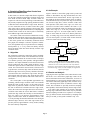
Dynamic Kernel Code Optimization1
Ariel Tamches
Barton P. Miller
VERITAS Software Corporation
350 Ellis Street
Mountain View, CA 94043-2237
Computer Sciences Department
University of Wisconsin
Madison, WI 53706-1685
[email protected]
[email protected]
Abstract
We have developed a facility for run-time optimization of a
commodity operating system kernel. Our infrastructure,
currently implemented on UltraSPARC Solaris 7, includes
the ability to do a detailed analysis of the running kernel's
binary code, dynamically insert and remove code patches,
and dynamically install new versions of kernel functions. As
a first use of this technology, we have implemented a runtime kernel version of the code positioning I-cache optimizations. We performed run-time code positioning on the kernel’s TCP read-side processing routine while running a Web
client benchmark, reducing the I-cache miss stall time of
this function by 35.4% and improved the function’s overall
performance by 21.3%.
The primary contributions of this paper are the first
run-time kernel implementation of code positioning, and an
infrastructure for run-time kernel optimizations. A further
contribution is made in performance measurement. We provide a simple and effective algorithm for deriving control
flow edge execution counts from basic block execution
counts, which contradicts the widely held belief that edge
counts cannot be derived from block counts.
1 Introduction
This paper studies dynamic optimization of a commodity
operating system kernel. We describe a mechanism for
replacing the code of almost any kernel function with an
alternate implementation, enabling installation of run-time
optimizations. As a proof of concept, we demonstrate a
dynamic kernel implementation of Pettis and Hansen’s code
positioning I-cache optimizations [10]. We applied code
positioning to Solaris TCP kernel code while running a Web
client benchmark, reducing the I-cache stall time of the TCP
read-side processing routine by 35.4%. This led to a 21.3%
speedup in each invocation of tcp_rput_data and a 7.1%
speedup in the benchmark’s elapsed run-time, demonstrating that even I/O workloads can incur enough CPU time to
benefit from I-cache optimization.
Pettis and Hansen implemented code positioning in a
feedback-directed customized compiler for user code,
applying the optimizations off-line and across an entire program. In contrast, our implementation is performed on ker-
nel code and entirely at run-time. The dynamic nature of our
infrastructure allows the optimization to be focused on a
desired portion of the kernel’s code; there is no need to optimize the entire system en masse, as is common with static
techniques.
Our implementation is the first on-line kernel version of
code positioning. In the bigger picture, our dynamic kernel
optimization framework is a first step toward evolving operating system kernels, which dynamically modify their code
at their own behest in response to their environment.
2 Algorithm
As a demonstration of the mechanisms necessary to support
an evolving kernel, we have implemented run-time kernel
code positioning within the KernInst dynamic kernel instrumentation system [15]. KernInst contains three components: a high-level GUI kperfmon which generates
instrumentation code for performance measurement, a lowlevel privileged kernel instrumentation server kerninstd, and
a small pseudo device driver /dev/kerninst which aids kerninstd when the need arises to operate from within the kernel’s address space. Kerninstd also performs a structural
analysis of the kernel’s machine code, calculating control
flow graphs and a call graph, as well as performing an interprocedural live register analysis.
We perform code positioning as follows: (1) A function
to optimize is chosen. This is the only step requiring user
involvement. (2) KernInst determines if the function has an
I-cache bottleneck. If so, basic block execution counts are
gathered for this function and its frequently called descendants. From these counts, a group of functions to optimize
is chosen. (3) An optimized re-ordering of these functions is
chosen and installed into the running kernel. Interestingly,
once the optimized code is installed, the entire code positioning optimization is repeated (once) – optimizing the
optimized code – for reasons discussed in Section 2.1.3.
2.1 Measurement Steps
The first measurement phase determines whether an I-cache
bottleneck exists, making code positioning worthwhile.
Next, basic block execution counts are collected for the
user-specified function and a subset of its descendants.
1. This work is supported in part by Department of Energy Grant DE-FG02-93ER25176, Lawrence Livermore National Lab grant B504964, NSF grants
CDA-9623632 and EIA-9870684, and VERITAS Software Corporation. The U.S. Government is authorized to reproduce and distribute reprints for Governmental purposes notwithstanding any copyright notation thereon.
Page 1
Code positioning is performed not only on the userspecified function, but also the subset of its call graph
descendants that significantly affects its I-cache performance. We call the collective set of functions a function
group; the user-specified function is the group’s root function. The intuitive basis for the function group is to gain
control over I-cache behavior while the root function executes. Because the group contains the hot subset of the root
function’s descendants, once the group is entered via a call
to its root function, control will likely stay within the group
until the root function returns.
2.1.1 Is There an I-Cache Bottleneck?
The first measurement step checks whether code positioning might help. KernInst instruments the kernel to obtain
the root function’s I-cache stall time and its CPU time. If
the ratio of these measurements is above a user-definable
threshold (10% by default), then the algorithm continues.
KernInst collects timing information for a desired code
resource (function or basic block) by inserting instrumentation code that starts a timer at the code’s entry point, and
stops the timer at the code’s exit point(s). The entry instrumentation reads and stores the current time, such as the processor’s cycle counter. The exit instrumentation re-reads the
time and adds the delta to an accumulated total. Changing
the underlying event counter that is read on entry and exit
(e.g. using the UltraSPARC I-cache stall cycle counter [14])
enables measurements other than timing.
Measurements made using this framework are inclusive;
any events that occur in calls made by the code being measured are included. This inclusion is vital when measuring
I-cache stall time, because a function’s callees contribute to
its I-cache behavior. By contrast, sampling-based profilers
can collect inclusive time measurements only by performing an expensive stack back-trace on each sample.
Another key aspect of this framework is that it accumulates wall time events, not CPU time events. That is, it continues to accumulate events when context switched out.
This trait is desirable for certain metrics (particularly I/O
latency), but not for metrics such as I-cache stall time and
CPU execution time. Fortunately, this problem can be
solved with additional kernel instrumentation – of the lowlevel context switch handlers – to exclude events that occur
while context-switched out. The complete version of this
paper [16] describes this process.
2.1.2 Collecting Basic Block Execution Counts
The second measurement phase performs a breadth-first call
graph traversal, collecting basic block execution counts of
any function that is called at least once while the root function is active (on the call stack). The block counts are used
to determine which functions are hot (these are included in
the group), and to divide basic blocks into hot and cold sets.
The traversal begins by dynamically instrumenting the
root function to collect its basic block counts. After the
instrumented kernel runs for a short time (the default is 20
seconds), the instrumentation is removed and the block
counts are examined. The set of statically identifiable
callees of this function then have their block counts measured in the same way. Pruning is applied to the call graph
traversal in two cases: a function that has already had its
block execution counts collected is not re-measured, and a
function that is only called from within a basic block whose
execution count is zero is not measured.
Because KernInst does not currently keep indirect function calls (i.e., through a function pointer) in its call graph, a
function called only indirectly will not have its block counts
measured. Ramifications are discussed in Section 5.4.
2.1.3 Measuring Block Counts Only When Called by
the Root Function
When collecting basic block execution counts for the root
function’s descendants, we wish to count only those executions that affect the root function’s I-cache behavior. In particular, a descendant function that is called by the root
function may also be called from elsewhere in the kernel
having nothing to do with the root function.
KernInst achieves this more selective block counting by
performing code positioning twice – re-optimizing the optimized code. Because code replacement, the installation of a
new version of a function (Section 3), is performed solely
on the root function, non-root group functions only are
invoked while the optimized root function is on the call
stack. This invariant ensures that measured block counts
during re-optimization include only executions when the
root function is on the call stack; instrumentation code need
not explicitly perform this check.
2.2 Choosing the Block Ordering: Code
Positioning
Among the functions whose basic block execution counts
were measured, the optimized group contains those with at
least one hot block. A hot basic block is one whose measured execution frequency, when the root function is on the
call stack, is greater than 5% of the frequency that the root
function is called. (The threshold is user-adjustable.)
Procedure splitting is performed first. Each group function is segregated into hot and cold chunks; a chunk is a
contiguous layout of either all of the hot, or all of the cold,
basic blocks of a function. We always place a function’s
entry block at the beginning of its hot chunk, for simplicity.
To aid optimization, not only are the hot and cold blocks
of a single function segregated, but all group-wide hot
blocks are segregated from the group-wide cold blocks. In
other words, procedure splitting is applied group-wide.
Basic block positioning chooses a layout ordering for
the basic blocks within a chunk. Edge execution counts,
Page 2
derived using the algorithm in Section 4, are used to choose
an ordering for a chunk’s basic blocks that facilitates
straight-lined execution in the common case. Through a
weighted traversal of these edge counts, each basic block of
the function’s hot chunk is placed in a chain, a sequence of
contiguous blocks that is optimized for straight-lined execution [10]. The motivation behind chains is to place the more
frequently taken successor block immediately after the
block containing a branch. In this way, some unconditional
branches can be eliminated. For a conditional branch, placing the likeliest of the two successors immediately after the
branch allows the fall-through case to be the more commonly executed path (after reversing the conditional being
tested by the branch instruction, if appropriate). In general,
the number of basic blocks (or instructions) in a chain gives
the expected distance between taken branches. The more
instructions between taken branches, the better the I-cache
utilization and the lower the mispredicted branch penalty.
Ideally, a function’s hot chunk is covered by a single chain.
2.3 Emitting and Installing the Optimized Code
After ordering the group’s contents, KernInst generates the
optimized code and installs it into the running kernel.
In order to emit functions with a new ordering, KernInst
first parses each function’s machine code into a relocatable
representation. Next, it emits the group code, which must be
relocatable, because its kernel address has not yet been
determined. Procedure calls are treated specially; if the
callee is a group function, then the call is redirected to the
group’s version of that function. Kerninstd then allocates
space for the code and resolves relocatable elements, much
like a dynamic linker. Further details are in the longer version of this paper [16].
After installation via code replacement (Section 3) on
the group’s root function, KernInst analyzes the group’s
functions like all other kernel functions. This analysis
includes parsing function control-flow graphs, performing a
live-register analysis, and updating the call graph. The firstclass treatment of runtime-generated code allows the new
functions to be instrumented (so the speedup achieved by
the optimization can be measured, for example) and even
re-optimized (a requirement, as discussed in Section 2.1.3).
3 Code Replacement
Code replacement is the primary mechanism that enables
run-time kernel optimization, allowing the code of any kernel function to be dynamically replaced (en masse) with an
alternate implementation.
Code replacement is implemented on top of KernInst’s
splicing primitive [15]. The entry point of the original function is spliced to jump to the new version of the function.
Code replacement takes about 68 µs if the original function
resides in the kernel nucleus and about 38 µs otherwise.
(The Solaris nucleus is a 4 MB range covered by a single
I-TLB entry.) If a single branch instruction cannot jump
from the original function to the new version of the function, then a springboard [15] is used to achieve sufficient
displacement. If a springboard is required, then a further
170 µs is required if the springboard resides in the nucleus,
and 120 µs otherwise.
The above framework incurs overhead each time the
function is called. This overhead often can be avoided, by
patching calls to the original function to directly call the
new version of the function. This optimization can be
applied for all statically identifiable call sites, but not to
indirect calls through a function pointer. Replacing one call
site takes about 36 µs if it resides in the nucleus, and about
18 µs otherwise. To give a large-scale example, replacing
the function kmem_alloc, including patching of its 466 call
sites, takes about 14 ms. Kernel-wide, functions are called
an average of 5.9 times, with a standard deviation of 0.8.
(This figure excludes indirect calls, which cannot be analyzed statically.)
The cost of installing the code replacement (and of later
restoring it) is higher than you might expect, because
/dev/kerninst performs an expensive undoable write for each
call site. Undoable writes are logged by /dev/kerninst, which
reverts code to its original value by if the front-end GUI or
kerninstd exit unexpectedly.
Kerninstd analyzes the replacement (new) version of a
function at run-time, creating a control flow graph, calculating a live register analysis, and updating the call graph in
the same manner as kernel code that was recognized at
kerninstd startup. This uniformity is important because it
allows tools built on top of kerninstd to treat the replacement function as first-class. For example, when kperfmon is
informed of a replacement function, it updates its code
resource display, and allows the user to measure and even
re-optimize the replacement function as any other.
Dynamic code replacement is undone by restoring the
patched call sites, then un-instrumenting the jump from the
entry of the original function to the entry of the new version. This ordering ensures atomicity; until code replacement undoing has completed, the replacement function is
still invoked due to the jump from the original to new version. Basic code replacement, when no call sites were
patched, is undone in 65 µs if the original function lies in
the nucleus, and 40 µs otherwise. If a springboard was used
to reach the replacement function, then it is removed in a
further 85 µs if it resided in the nucleus, and 40 µs otherwise. Each patched call site is restored in 30 µs if it resided
in the nucleus, and 16 µs otherwise.
Page 3
4 Calculating Edge Execution Counts from
Block Execution Counts
4.2 An Example
In this section, we describe a simple and effective algorithm
for deriving control flow graph edge execution counts from
basic block execution counts. Edge execution counts are
required for effective block positioning, but KernInst does
not presently implement an edge splicing mechanism which
would allow direct measurement of edge counts. However,
we have found that 99.6% of Solaris control flow graph
edge counts can be derived from basic block counts. This
result implies that simple instrumentation (or sampling) that
measures block counts can be used in place of technically
more difficult edge count measurements.
The results of this section tend to contradict the widelyheld belief that while block counts can be derived from edge
counts, the converse does not hold. Although that limitation
is true in the general case of arbitrarily structured control
flow graphs, our technique is effective in practice. Furthermore, the algorithm may be of special interest to samplingbased profilers [1, 7, 8, 18], which can directly measure
block execution counts but cannot directly measure edge
execution counts.
Figure 1 contains a control flow graph used by Pettis and
Hansen to demonstrate why edge measurements are more
useful than block measurements. Precise edge counts for
this graph can be derived from its block counts, as follows.
First, block B has only one predecessor edge (A,B) and only
one successor edge (B,D), whose execution counts must
each equal B’s count (1000). Now, edge (A,C) is the only
successor of A whose count is unknown. Its count is 1 (A’s
count of 1001 minus the count of its known successor edge,
1000). Next, edge (C,C) is the only remaining unknown
predecessor edge of C. Its count equals 2000 (C’s block
count of 2001 minus the count of its known predecessor
edge, 1). Finally, edge (C,D) is the only unknown successor
of C. Its count equals 1 (C’s block count of 2001 minus the
count of its known successor edge, 2000).
A
block count=1001
1000
2000
1
B
C
block count=1000
block count=2001
4.1 Algorithm
1000
We assume that a function’s control flow graph is available,
along with execution counts of the function’s basic blocks.
Our algorithm calculates the execution counts of all edges
of a function, precisely when possible, and approximated
otherwise. Two simple formulas are used: the sum of a basic
block’s predecessor edge counts equals the block’s count,
which also equals the sum of that block’s successor edge
counts. For a block whose count is known, if all but one of
its predecessor (successor) edge counts are known, then the
unknown edge count can be precisely calculated: the block
count minus the sum of the known edge counts. The algorithm repeats until convergence, after which all edge counts
that could be precisely derived from block counts were so
calculated.
The second phase of the algorithm approximates any
remaining, unknown edge execution counts. Two formulas
bound the count of such an edge: (1) the count can be no
larger than its predecessor block’s execution count minus
the sum of that block’s calculated successor edge counts,
and (2) the count can be no larger than its successor block’s
execution count minus the sum of that block’s calculated
predecessor edge counts. We currently use the minimum of
these two values as an imprecise approximation of that
edge’s execution count. There are alternative choices, such
as evenly dividing the maximum allowable value among all
unknown edges. However, since most edge counts can be
precisely derived, approximation is rarely needed, making
the issue relatively unimportant.
1
D
block count=1001
Figure 1: Deriving Edge Counts From Block Counts
The count for edge (X, Y) can be calculated if it is the only
unknown successor count of block X, or the only unknown
predecessor count of block Y. Repeated application can often
calculate all edge counts, as in this example (an augmented
Figure 3 from [10]).
4.3 Results and Analysis
Applying the above algorithm to the Solaris kernel reveals
that 99.6% of its control flow graph edge counts can be
derived from basic block counts. Furthermore, for 97.8% of
kernel functions, we can precisely calculate counts for every
one of their control flow graph edges. Thus, with few exceptions, collecting block counts is sufficient to derive edge
counts. This conclusion is especially useful for samplingbased profilers, which cannot directly measure edge counts.
Even where edge counting can be directly measured,
deriving edge counts from block counts may be preferable
because sampling can make it less expensive. For example,
dcpi [1] obtains accurate measurements by sampling 5200
times per second, yet the system overhead is only 1-3%.
Page 4
5 Experimental Results
As a concrete demonstration of the efficacy of run-time kernel code positioning, this section presents initial results in
optimizing the I-cache performance of the Solaris kernel
while running a Web client benchmark. We study the performance of tcp_rput_data (and its callees), which processes
incoming network data. tcp_rput_data is called thousands of
times per second in the benchmark, and has poor I-cache
performance: about 36% of its time is spent in I-cache
misses. Using our prototype implementation of code positioning, we reduced the time per invocation of tcp_rput_data
in our benchmark from 6.6 µs to 5.44 µs, a speedup of
21.3%. (We concentrate on optimizing the per invocation
cost of tcp_rput_data, to achieve an improvement that scales
with its execution frequency.)
5.1 Benchmark
We used the GNU wget tool [6] to fetch 34 files totaling
about 28 MB of data, largely comprised of Postscript, compressed Postscript, and PDF files. The benchmark contained
ten simultaneous connections, each running the wget program as described over a 100 MB/sec LAN. The client
machine had a 440 MHz UltraSPARC-IIi processor.
The benchmark spends much of its time in the read side
of TCP code, especially tcp_rput_data. We chose to perform
code positioning on tcp_rput_data because of its size (about
12K bytes of code across 681 basic blocks), which suggests
there is room for I-cache improvement.
5.2 tcp_rput_data Performance: Before
other words, tcp_rput_data spends about 36% of its execution time in I-cache miss processing.
The measured basic block execution counts of
tcp_rput_data and its descendants estimate the hot set of
basic blocks during the benchmark’s run. The measured
counts are an approximation, both because code reached via
an indirect call is not measured, and because the measurement includes block executions without regard to whether
the group’s root function is on the call stack. These approximate block counts were used to estimate the likely I-cache
layout of the subset of these blocks that are hot (those which
are executed over 5% as frequently as tcp_rput_data is
called). The estimate is shown in Figure 2a.
Two conclusions about I-cache performance can be
drawn from Figure 2a. First, having greater than 2-way set
associativity in the I-cache would have helped, because the
hot subset of tcp_rput_data and its descendants cannot execute without I-cache conflict misses. Second, even if the
I-cache were fully associative, it may be too small to effectively run the benchmark. The bottom of Figure 2a estimates that 244 I-cache blocks (about 7.8K) are needed to
hold the hot basic blocks of tcp_rput_data and its descendants, which is about half of the total I-cache size. Because
other code, particularly Ethernet and IP processing code
that invokes tcp_rput_data, is also executed thousands of
times per second, the total set of hot basic blocks likely
exceeds the capacity of the I-cache.
5.3 tcp_rput_data Performance: After
To determine whether tcp_rput_data is likely to benefit from
code positioning, we measured the inclusive CPU time that
it spends in I-cache misses. The result is surprisingly high;
each invocation of tcp_rput_data takes about 6.6 µs, of
which about 2.4 µs is idled waiting for I-cache misses. In
We performed code positioning to improve the inclusive
I-cache performance of tcp_rput_data. Figure 2b presents
the I-cache layout of the optimized code, estimated in the
same way as in Figure 2a. There are no I-cache conflicts
among the group’s hot basic blocks, which could have fit
comfortably within an 8K direct-mapped I-cache.
0 0 0 0 1 1 1 0 1 1 0 0 0
1 1 2 2 2 2 2 2 2 1 1 1 1
1 1 1 2 2 2 1 0 0 0 0 0 1
1 1 1 1 1 1 1 1 1 1 1 0 0
0 0 1 1 2 0 1 1 3 2 2 1 1
2 2 0 0 0 0 0 1 1 1 1 2 2
2 1 1 2 2 2 0 1 1 3 3 3 3
1 3 2 1 1 0 1 1 1 0 0 0 0
0 0 0 2 1 1 1 1 1 1 1 1 1
2 2 3 2 2 1 2 2 1 0 0 1 1
1 0 0 0 0 0 0 0 0 0 1 0 0
0 0 0 0 0 0 0 1 0 1 0 0 1
1 1 0 0 0 0 0 0 0 0 1 0 0
0 0 0 0 1 2 1 1 1 1 2 2 1
3 3 4 4 4 3 4 4 4 3 2 1 0
0 0 0 0 0 0 0 1 1 1 1 0 0
Total # of cache blocks: 244 (47.7% of the I-Cache size)
(a) Before Optimization
0 1 1 1 1 1 1 1 1 1 1 1 1
1 1 1 1 1 1 1 1 1 1 1 1 1
1 1 1 1 1 1 1 1 1 1 1 1 1
1 1 1 1 1 1 1 1 1 1 1 1 1
1 1 1 1 1 1 1 1 1 1 1 1 1
1 1 1 1 1 1 1 1 1 1 1 1 1
1 1 1 1 1 1 1 1 1 1 1 1 1
1 1 1 1 1 1 1 1 1 1 1 1 1
1 1 1 1 1 0 0 0 0 0 0 0 0
0 0 0 0 0 0 0 0 0 0 0 0 0
0 0 0 0 0 0 0 0 0 0 0 0 0
0 0 0 0 0 0 0 0 0 0 0 0 0
0 0 0 0 0 0 0 0 0 0 0 0 0
0 0 0 0 0 0 0 0 0 0 0 0 0
0 0 0 0 0 0 0 0 0 0 0 0 0
0 0 0 0 0 0 0 0 0 0 0 0 0
Total # of cache blocks: 132 (25.8% of the I-Cache size)
(b) After Optimization
1
1
2
0
1
2
1
0
0
1
0
0
0
2
2
0
2
1
2
0
1
1
2
0
0
1
0
1
0
1
2
0
2
0
1
0
1
2
3
0
1
1
0
1
0
2
1
0
1
1
1
1
1
1
1
1
0
0
0
0
0
0
0
0
1
1
1
1
1
1
1
1
0
0
0
0
0
0
0
0
Figure 2: I-cache Layout of the Hot Blocks of tcp_rput_data and its Descendants (Before and After Optimization)
Each cell represents a 32-byte I-cache block with a count of how many hot basic blocks with distinct I-cache tags, reside there. The
UltraSPARC I-cache is 16K, 2-way set associative; highlighted cells (those with counts greater than two) indicate a likely conflict.
Page 5
1
1
1
1
1
1
1
1
0
0
0
0
0
0
0
0
Figure 3 shows the functions in the optimized group
along with the relative sizes of the hot and cold chunks. The
figure demonstrates that procedure splitting is effective,
with 77.4% of the group’s code consisting of cold basic
blocks. Block positioning is also effective, with the hot
chunk of most group functions covered by a single chain.
Function
tcp/tcp_rput_data
unix/mutex_enter
unix/putnext
unix/lock_set_spl_spin
genunix/canputnext
genunix/strwakeq
genunix/isuioq
ip/mi_timer
ip/ip_cksum
tcp/tcp_ack_mp
genunix/pollwakeup
genunix/timeout
genunix/.div
unix/ip_ocsum
genunix/allocb
unix/mutex_tryenter
genunix/cv_signal
genunix/pollnotify
genunix/timeout_common
genunix/kmem_cache_alloc
unix/disp_lock_enter
unix/disp_lock_exit
Totals
Jump
Table
Data
56
0
0
0
0
0
0
0
0
0
0
0
0
0
0
0
0
0
0
0
0
0
56
Hot # Chains Cold
Chunk in Hot Chunk
bytes
Chunk bytes
1980
44
160
32
60
108
40
156
200
248
156
40
28
372
132
24
36
64
204
112
28
36
4260
10
1
1
1
1
1
1
1
1
1
1
1
1
4
1
1
1
1
1
1
1
1
34
11152
0
132
276
96
296
36
168
840
444
152
0
0
80
44
20
104
0
52
700
12
20
14624
Figure 3: The Optimized tcp_rput_data Group
The group contains a new version of tcp_rput_data, and the hot
subset of its statically identifiable call graph descendants, with
code positioning applied. The group’s layout consists of 56 bytes of
jump table data, followed by 4,260 bytes of hot code, and finally
14,624 bytes of cold code. (Although mutex_enter is in the group,
mutex_exit is not, because a Solaris trap handler tests the PC
register against mutex_exit’s code bounds. To avoid confusing this
test, KernInst excludes mutex_exit from group code.)
Code positioning resulted in a 7.1% speedup in the
benchmark’s end-to-end run-time, from 36.0 seconds to
33.6 seconds. To explain the speedup, we used kperfmon to
measure the performance improvement in each invocation
of tcp_rput_data. Pre- and post-optimization numbers are
shown in Figure 4.
5.4 Analysis of Code Positioning Limitations
Code positioning performs well unless there are indirect
function calls among the hot basic blocks of the group. This
section analyzes the limitations that indirect calls placed on
the optimization of tcp_rput_data (and System V streams
code in general), to quantify how the present inability to
optimize across indirect calls constrains code positioning.
The System V streams code has enough indirect calls to
limit what can presently be optimized to a single streams
Measurement
I-$ stall time/invoc
Branch mispredict
stall time/invoc
IPC (instrucs/cycle)
Original
2.40 µs
Optimized
1.55 µs
Change
0.38 µs
0.20 µs
-47.4%
0.28
0.38
+35.7%
6.60 µs
5.44 µs
21.3% speedup
CPU time/invoc
-35.4%
Figure 4: Measured Performance Improvements in
tcp_rput_data After Code Positioning
The performance of tcp_rput_data has improved by 21.3%, mostly
due to fewer I-cache stalls and fewer branch mispredict stalls.
module (TCP, IP, or Ethernet). Among the measured hot
code of tcp_rput_data and its descendants, there are two frequently-executed indirect function calls. Both calls are
made from putnext, a stub routine that forwards data to the
next upstream queue by indirectly calling the next module’s
stream “put” procedure. This call is made when TCP has
completed its data processing (verifying check sums and
stripping off the TCP header from the data block), and is
ready to forward the processed data upstream. Because
callees reached by hot indirect function calls cannot currently be optimized, we miss the opportunity to include the
remaining upstream processing code in the group. At the
other end of the System V stream, by using TCP’s data processing function as the root of the optimized group, we
missed the opportunity to include downstream data processing code performed by the Ethernet and IP processing.
Across the entire kernel, functions make an average of
6.0 direct calls (standard deviation 10.6) and just 0.2 indirect calls (standard deviation 0.8). However, because indirect calls tend to exist routines that are invoked throughout
the kernel, any large function group will likely contain at
least one such call.
6 Related Work
6.1 Measurement
An alternative to our instrumentation is sampling [1, 7, 8,
18]. Sampling measures CPU time events by periodically
reading the PC, and assigning the time since the last sample
at that location. Although it is simple and has constant perturbation, sampling has several limitations. First, modern
CPUs having imprecise exceptions with variable delay may
require hardware support to accurately assign events to
instructions [5]. Second, while sampling can measure CPU
time, it can only measure wall time with a prohibitive call
stack back-trace of all blocked threads per sample. Third,
sampling can only measure inclusive metrics by assigning
time for all routines on the call stack for each sample. Aside
from the expense, stack back-traces can be inaccurate due to
tail-call optimizations, in which a caller removes its stack
frame (and thus its call stack entry) before transferring control to the callee. Tail-call optimizations are common, found
about 3,800 times in Solaris kernel code.
Page 6
6.2 Dynamic Optimization
References
Previous work has been performed on I-cache kernel optimization of kernel code [9, 12, 13, 17], although the focus
has been on static, not dynamic, optimization.
Dynamo [2] is a user-level run-time optimization system
for HP-UX programs. Dynamo initially interprets code to
collect hot instruction sequences, which are then placed in a
software cache for execution at full speed. Similar in spirit
to KernInst’s evolving framework, Dynamo has several differences. First, it only runs on user-level code. It would be
difficult to port Dynamo to a kernel because interpreting a
kernel is more difficult. Even if possible, the overhead of
kernel interpretation may be unacceptable, because the
entire system is affected by a kernel slowdown. Second,
Dynamo expands entire hot paths, so the same basic block
can appear multiple times. This expansion can result in a
code explosion when the number of executed paths is high.
The PA8000 on which Dynamo runs may be able to handle
code explosion, because it has an unusually large I-cache
(1 MB). The same is not likely to be true for the UltraSPARC-II’s 16K I-cache.
Synthetix [11] performs specialization on a modified
commodity kernel. However, it requires specialized code
templates to be pre-compiled into the kernel. Synthetix also
requires a pre-existing level of indirection (a call through a
pointer) to change implementations of a function, which
incurs a slight performance penalty whether or not specialized code has been installed, and limits the number of
points that can be specialized.
[1] J.M. Anderson et al. Continuous Profiling: Where Have All
the Cycles Gone? 16th ACM Symp. on Operating System
Principles (SOSP), Saint-Malo, France, October 1997.
[2] V. Bala, E. Duesterwald, and S. Banerjia. Dynamo: A
Transparent Dynamic Optimization System. ACM SIGPLAN
Conf. on Programming Language Design and Implementation
(PLDI), Vancouver, BC, June 2000.
[3] H. Cain, B.P. Miller, and B.J.N. Wylie. A Callgraph-Based
Search Strategy for Automated Performance Diagnosis.
European Conf. on Parallel Computing (Euro-Par), Munich,
Germany, August 2000.
[4] R. Cohn and P.G. Lowney. Hot Cold Optimization of Large
Windows/NT Applications. IEEE/ACM International Symp.
on Microarchitecture (MICRO-29), Paris, December 1996.
[5] J. Dean, et. al. ProfileMe: Hardware Support for InstructionLevel Profiling on Out-of-Order Processors. 30th Annual
IEEE/ACM International Symp. on Microarchitecture
(MICRO-30), Research Park Triangle, NC, December 1997.
[6] Free Software Foundation. GNU wget: The Non-Interactive
Downloading Utility.
http://www.gnu.org/software/wget/wget.html.
[7] S.L. Graham, P.B. Kessler, and M.K. McKusick. gprof: a Call
Graph Execution Profiler. SIGPLAN 1982 Symp. on Compiler
Construction, Boston, MA, June 1982.
[8] Intel Corporation. VTune Performance Analyzer 4.5.
7 Future Work
Our basic block counting overhead could be lowered by
combining block sampling and Section 4’s algorithm for
deriving edge counts. We note that KernInst’s optimization
is orthogonal to the means of measurement, because the
logic for analyzing machine code, re-ordering it, and installing it into a running kernel is orthogonal to how the new
ordering is obtained.
With additional kernel instrumentation at indirect call
sites, the call graph can be updated when a heretofore
unseen callee is encountered, allowing indirect callees to be
included in an optimized group [3].
User involvement in choosing the group’s root function
can be removed by automating the search for functions having poor I-cache performance. Such a search can be performed by traversing the call graph using inclusive
measurements [3].
Because non-root group functions are always invoked
while the root function is on the call stack, certain invariants
may hold that enable further optimizations [4]. For example, a variable may be constant, allowing constant propagation and dead code elimination. Other optimizations include
inlining, specialization, and super-blocks.
http://developer.intel.com/vtune/analyzer/index.htm.
[9] D. Mosberger et. al. Analysis of Techniques to Improve
Protocol Processing Latency. ACM Applications,
Technologies, Architectures and Protocols for Computer
Communication (SIGCOMM), Stanford, CA, August 1996.
[10] K. Pettis and R.C. Hansen. Profile Guided Code Positioning.
ACM SIGPLAN Conf. on Programming Language Design and
Implementation (PLDI), White Plains, NY, June 1990.
[11] C. Pu, et. al. Optimistic Incremental Specialization:
Streamlining a Commercial Operating System. 15th ACM
Symp. on Operating Systems Principles (SOSP), Copper
Mountain, CO, December 1995.
[12] W.J. Schmidt et. al. Profile-directed Restructuring of
Operating System Code. IBM Systems Journal 37(2), 1998.
[13] S.E. Speer, R. Kumar, and C. Partridge. Improving UNIX
Kernel Performance Using Profile Based Optimization. 1994
Winter USENIX Conf., San Francisco, CA, 1994.
[14] Sun Microsystems. UltraSPARC-IIi User’s Manual.
www.sun.com/microelectronics/manuals.
[15] A. Tamches and B.P. Miller. Fine-Grained Dynamic
Instrumentation of Commodity Operating System Kernels.
3rd USENIX Symp. on Operating Systems Design and
Implementation (OSDI), New Orleans, LA, February 1999.
[16] A. Tamches and B.P. Miller. Dynamic Kernel Code
Optimization. 3rd Workshop on Binary Translation (WBT).
Barcelona, Spain, September 2001.
[17] J. Torrellas, C. Xia, and R. Daigle. Optimizing the Instruction
Cache Performance of the Operating System. IEEE
Transactions on Computers, 47(12), December 1998.
[18] X. Zhang, et. al. System Support for Automatic Profiling and
Optimization. 16th ACM Symp. on Operating System
Principles (SOSP), Saint-Malo, France, October 1997.
Page 7