Download Using a Manufacturer`s Specification as a Type B Error Contribution

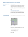
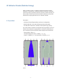
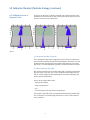
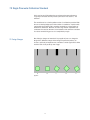
Using a Manufacturer’s Specification
as a Type B Error Contribution
White Paper
Robert L Brown, Agilent Technologies
Presented at 2006 NCSL International Workshop and Symposium
Abstract
Manufacturers’ specifications are a complicated interplay of consumer demand,
contractual agreement and definition of “fitness for use” warranty. To better
understand the implications of using manufacturers’ specifications in an uncertainty analysis, we will explore technical topics such as the following ...
• How specifications are created and managed
• Advantage of using specification
• Statistic versus managed specification
• Stationary and non-stationary random processes
• GUM concepts like “safe”
• Issue and definition of pseudo systematic error
This exploration will be done using no advanced math or statistics. This paper
examines these issues in the informal context of a Pachinko gambling device.
As a result, it will become clear why an uncertainty analysis (employing TYPE B
data) is a worst case analysis. This can affect how calibration laboratories use
uncertainty data in the quality system and on customer facing documents and
training.
1.0 Introduction
Why are manufacturers’ specifications allowed in uncertainty calculation regimens such as those discussed in GUM and E4/02? The answer is simply, “convenience.” A full ANOVA would require very specific knowledge about modern
standards. Much of this paper is dedicated to the types of error contributions
that are encapsulated in manufacturers’ specifications. These ideas are presented in a way that makes very complicated subjects easier to communicate.
2.0 Nature of a Manufacturers’ Specification
It is important to be aware of the conflict between manufacturers’ needs and
those of a metrologist seeking a statistic.
2.1 Manufacturers’ Needs
The manufacturer needs to communicate the definition of “fitness for use.”
2.2 Customers’ (End User)
Needs
The customer wants to depend upon the manufacturer’s specification. The
customer needs to know (User Manual) how to get the promised performance
and what obligations that he has (environment, calibration interval, etc.). The
customer wants to be able to substitute a “stock” instrument in his system
with confidence that it will perform as well as the one replaced. The customer
often wants a maintenance contract. Product specifications provide the required
“meeting of the minds” to indicate those repairs that are (or are not) covered by
that maintenance contract.
2.3 Metrologists’ Uncertainty
Needs
When using specifications as Type B contributors, metrologists’ needs are the
same as the End User (2.2). However, if an application uses characterized data
to obtain better performance than published specifications, then that application
is not supported by the manufacturer (and is beyond the scope of this paper).
However, some of the concepts in this paper are useful for those characterized
applications.
2.4 Managed Specifications
The specification is therefore a promise. Manufacturers do collect statistics
as they design for manufacturing. However, in the end, the manufacturer must
decide what he can promise to deliver for a period of many years. In section
7.0 we will discuss the incredibly large margins required to make that promise
cost effective. GUM [1] sections E.2.1 and E.2.2, make a case for a realistic
uncertainty with a confidence interval. However, the use of specifications in
an uncertainty analysis will in most cases make the analysis conservative (and
in conflict with E.2). It is impossible to predict, at the time the specification
is defined, when and for which (future) serial numbers the specification will
be realistic. The flexibility that is afforded to manufacturing (due to process
margins Cpk and Cp) actually makes the price of many modern standards (especially multi-parameter) much less expensive. Robust engineering designs allow
manufacturing to make the promise, and manage to the specification.
2
3.0 Pachinko Machine Error Contribution Types
To identify the major types of error contributions, we will examine a device
designed to create randomness: the Pachinko gambling machine. We will identify types by how they need to be handled rather than by source or root cause.
This discussion will emphasize the difficult issue of “time.”
3.1 Pachinko Machine Metrics
For our analysis purposes (Figure 1A) the machine will be outfitted with a coordinate system. The horizontal scale is in units of peg spacing. Note that zero
indicates the initial position of every ball that is dropped into the array of pegs.
The vertical scale is in units of months, Jan = 1, Feb = 2, etc.
3.2 Combined Uncertainty
When describing randomness, we will consider one sigma numbers in this
example. The question to answer is, “What is the combined uncertainty of
the machine?” A Pachinko machine (Figure 1A) features a binning mechanism
that creates a histogram of Pachinko balls. You can see by inspection that the
standard deviation is approximately 3.9 units.
A
Figure 1.
3
B
3.0 Pachinko Machine Error Contribution Types (continued)
3.3 Potential Variation Shapes
Uncertainty in the actual path of a ball is represented graphically by a dark
shaded shape. The top of the shape indicates the assumed entry point. The
width of the base of the shape indicates the standard uncertainty of the exit.
The names given (Figure 1B) to these shapes were chosen to make the analogy
to a calibration standard more convenient later in this paper. The line down the
center indicates the expected (most likely) path of the ball. When the analogy is
complete, and an infinitely dense lattice of pegs is assumed, this expected path
is a straight line.
3.3.1 Calibration Shape
The top (Figure 1B) shape (isosceles triangle) indicates that a ball that enters at
the top (they all do) will be distributed at the bottom by a standard uncertainty
indicated by the width of the base. The base was calculated by making a table
of the space into which the first 100 balls fell. (The two most likely spaces
got the value 0.5, the next 1.5, etc). Then the standard deviation of those 100
observations was calculated to be 2.32 units. The width of the base reflects this
value. For the purpose of analogy, the vertical distance is not interesting in units
of time. The shape only indicates the input and the output of the calibration
process.
3.3.2 Drift Shape
The middle (Figure 1B) shape (dome) indicates the randomness in a ball’s path
caused by the pegs. The base width was calculated in a similar way to the
calibration uncertainty. The 100 data points indicated where a ball exited the
maze relative to the space that it entered. Then the standard deviation of those
100 observations was calculated to be 2.91 units. The width of the base reflects
this value.
In this shape, the vertical distance is significant and measured in units of
months. The dome shape is also significant. We know that the ball is equally
likely to move left or right at each peg. If the ball never moved more than one
space left or right then the result of this path is the Binomial Distribution and
the variance of the drift shape would be np(1-p) = n/4. However, it is clear from
watching the simulation that horizontal motion of multiple spaces is common.
As long as the expected (average) horizontal motion is constant, the variance
will increase linearly with n. Since we are indicating the standard deviation, the
dome shape width indicates that standard deviation at each height.
Sigma = SQRT(2.415 * t)
where t is in months
4
Equation 1
3.0 Pachinko Machine Error Contribution Types (continued)
3.3 Potential Variation Shapes
(continued)
3.3.3 Reproducibility Shape
The lower (Figure 1B) shape (isosceles triangle) indicates the randomness in
a ball’s path exiting the pegs at an other than vertical angle. Note that there
is additional uncertainty caused by the histogram binning. As in the previous
cases, a table of 100 values was constructed by noticing which bin captured the
ball. The value is the horizontal displacement of the bin relative to the space
where the ball exited the lattice. The width of the base reflects the standard
deviation of the 100 observations. The vertical distance is not significant in units
of time.
3.3.4 Total Combined Standard Uncertainty Bar
The shaded bar at the bottom indicates the combined effect of the three
Potential Variation Shapes discussed above. The width of this bar is simply the
RSS (root sum of squares) combination of the three standard uncertainties,
approximately 3.9 units as expected.
3.4 Using Potential Variation
Shapes
What if we repeatedly drop balls into the middle of the lattice? Can we use what
we have learned to predict the result?
Figure 2.
What if we drop balls into the lattice at the X (Figure 2) on the 15th of March.
What will be the Combined Standard Uncertainty of the Total result?
• There will be no Calibration contributor
• The Drift contribution will be 1 month’s worth;
(Equation 1) UD = SQRT(2.415 * 1) = 1.55
• The Repeatability will be as in 3.3.3, UR = 1.1
Total sigma = SQRT(UD2 + UR2) = 1.9 units
The mean = –5 units
5
4.0 Calibration Standard (Pachinko Analogy)
Unlike a Pachinko machine, a calibration standard is designed to minimize
randomness. The purpose of a calibration standard is to preserve a parameter.
It needs to transport a parameter value from one place to another and from one
time to another. We will use the obvious Pachinko randomness to help model
the difficult to manage, tight tolerances of a calibration standard.
4.1 Simple Model
Assumptions:
• Calibration, Drift and Reproducibility contributors are independent
• No (left/right) bias in the random walk (peg symmetry horizontally)
• The drift/time random walk is relatively constant (uniform peg spacing)
As a result of these assumptions, the expected value of population is zero error.
If these same assumptions are appropriate for a calibration standard that you
use or manufacture, then the Pachinko model will apply to that standard also.
Expected Value = Mean = 0
Combined Standard Uncertainty = SQRT(UC2 + UD2 +UR2)
where UD = SQRT(k * t), t = cal interval and k = (variance at t = 1)
A
Figure 3.
6
B
4.0 Calibration Standard (Pachinko Analogy) (continued)
4.1 Simple Model (continued)
To help adapt to the Calibration Standard, we will allow only a small number of
balls. Each ball will be stenciled with a year, beginning with year 2000 and ending this year. (Figure 3B) This models a calibration standard that was purchased
and calibrated Jan 1, 2000. With a calibration standard we get to drop only one
single ball each year on Jan 1 (beginning of the one year calibration cycle).
Figure 4.
4.2 Pseudo Systematic Error
Customers who use this standard earlier in the year will experience less pseudo
systematic error than near the end of the calibration cycle (Figure 4). In this
model, the actual value of the standard was low by 7 units on July 15, 2000 but,
4 units high on July 15, 2001. The user has no way of knowing the actual error.
The user will believe that the standard is still accurate with a visible random
variation, equal to the reproducibility contribution. The pseudo systematic error
appears to be trapped in time and is sometimes referred to as a “time trap”.
For novice metrologists, Pseudo Systematic errors are easier to grasp than the
concept of random variables in the frequency domain.
In the absence of Delta Environment Systematic Errors (4.3.3), total Pseudo
Systematic Error can be measured, with an uncertainty of the calibration contribution. This is the motivation for time series analysis of the “incoming” data
from the calibration reports.
Keep in mind, that the calibration contribution includes a component similar to
the Reproducibility component and time traps of its own. If the traceability path
is very long, you could easily be getting a value from the Standards Lab that was
sampled at the National Laboratory many years ago.
7
4.0 Calibration Standard (Pachinko Analogy) (continued)
4.3 Full Model (Inclusion of
Systematic Error)
In practice, the design of a calibration standard must include systematic errors.
Systematic errors are those errors that cause the expected (or mean) error to be
non-zero. Those errors are of three types.
A
B
C
Figure 5.
4.3.1 Asymmetric Drift Bias: (Figure 5A)
This is analogous to pegs that are slightly off center. This bias is related to the
size of the drift uncertainty (look up binomial distribution). Since there is no way
to distinguish this linear drift (due to Asymmetric Drift Bias) from non-random
drift (4.3.2), it is recommended that asymmetric random drift never be assumed.
4.3.2 Non-random Drift: (Figure 5B)
Non-random drift without an associated random drift is analogous to binding the
pegs into chutes, using wire. This can be considered to be the regression function (as in linear regression) when separating the random drift (residuals) from
the non-random drift (function).
Sources of non-random drift include:
• Aging of the standard
• Wear-out mechanisms
• Use
• Tension releasing from last mechanical adjustment
The example in Figure 5B shows non-random drift dominating the random drift.
This can happen in a standard weight. Each time it is used, a small amount of
mass is removed.
8
4.0 Calibration Standard (Pachinko Analogy) (continued)
4.3 Full Model (Inclusion of
Systematic Error) (continued)
4.3.3 Offset: (Figure 5C)
This type of systematic error, represented in Figure 5C, cannot be realized with
pegs and balls as depicted. However, the figure does better communicate the
nature of the offset error in a calibration standard. In a balls and pegs machine,
it would be an offset in the top and bottom scales in the diagram.
The illustration in Figure 5C was chosen to emphasize that Offset should be
considered the non-random calibration error contributor. This reminds us that
the most difficult and often undiagnosed Offset errors are “Delta Environment”
errors.
Sources of Delta Environment errors include:
• Equipment used at a different temperature, humidity, or altitude than when
calibrated
• Uncorrected offsets when used that were corrected when calibrated
• Procedure for using the standard is very different than the calibration
procedure used
The full model will include a constant term that represents the offset error.
4.3.4 Full Model Error Equation
Summarizing what has been said above,
Error( t ) = EO + E * t + C + D + R
Equation 2
EO = Delta Environment and uncorrected offsets (often assumed = 0)
E = Systematic drift of the standard (often assumed = 0)
C = Calibration random variable with expectation = 0, sigma = UC
D = Drift random variable with expectation = 0, sigma = UD = SQRT(k * t)
R = Reproducibility random variable with expectation = 0, sigma = UR
If we could know (we can’t) the value of each term at the precise instant, t, that
a standard is used, then we would have the exact error and know the “true”
value spoken about in GUM.
9
5.0 Using a Calibration Standard
When a calibration laboratory uses GUM to estimate the uncertainties of the
calibration procedures, it is required to:
1.Identify the significant systematic errors
2.Correct the significant systematic errors
3.Add an error contribution for each of the correction factors
Random errors are to be expected values, not “safe” or worst case.
5.1 Systematic Errors
To the extent that some systematic errors are “hidden” in the manufacturer’s
specification, this requirement cannot always be met. For example, there is
usually a temperature requirement in the user manual, but no indication of the
amount or direction of the error when using the calibration standard near the
edge of the requirement.
5.2 Random Errors
In practice, no one recommends that the expected value of the drift component
be used, even if it is the dominant contributor. If the expected value were used,
then the variance, UD(t)2, would be multiplied by the probability distribution of
calibration events, P(t), and integrated over the standard’s calibration interval
to obtain the expected drift variance (the expected value of the variance is an
unbiased estimator).
If (as is most common) the standard is used uniformly throughout the year,
then the corrected UD is given by UD/SQRT(2). In fact, no one objects to using
the worst case UD and many would likely object to this reduction in favor of the
worst case number.
10
6.0 Multi-Function Electronic Standards
Multiple parameters can effect the uncertainty budget in subtle ways.
6.1 Accumulated Effect of
Many Uncorrelated Parameters
To illustrate the problem of multiple sources for error, let’s consider a multifunction voltmeter. Assume that the specification for each functional parameter
is 95% confidence. Remember that only one parameter needs to fail to get an
Out Of Tolerance for the entire box. If each of the 100 parameters was uncorrelated with the others, then the expected number of failures per calibration
would be 5. This won’t do. All functioning boxes will fail “incoming” data when
in for calibration.
It is easy to see that for confidence of 95%, each of the 100 independent
parameters would require: Parameter Confidence = 0.95(1/100) = 0.950.01 = 0.99949.
This problem is mitigated in the design by making the parameters correlated. A
good example is a self-calibrating multimeter or calibrator that depends primarily
on the accuracy of only 2 high precision (internal) standards and an extremely
linear A/D converter. This multi-function dynamic is one of the reasons that
the true performance is typically much better than the product specification.
A single parameter may have a budget tighter than the parameter’s published
specification.
6.2 Highly Correlated
Parameters
To illustrate the problem of correlated sources for error, let us consider the
flatness of a radio frequency standard. Suppose that adjustment of the highest
frequency gain is correlated with the lowest frequency in that band. If the
calibration procedure can only minimize the difference (but never achieve zero),
then the adjustment of absolute gain may (by design) require one parameter to
be high and the other low. This offset, in effect, removes that difference from
the available specification budget.
11
7.0 Single Parameter Calibration Standard
In this section we will be explore the second reason that true performance
is typically much better than the product specification. That reason is, “the
unknown.”
The manufacturer has a similar problem to that of a calibration procedure. Both
have an uncertainty budget and a finite number of contributors. A product with
cutting-edge specifications (like a metrology standard) has a large number of
known error contributors. But there are also a large number of potential error
contributors that may be unknown. Accommodation of the unknown contributor
in a robust manufacturing process is accomplished by margin.
7.1 Design Changes
Not all design changes are intentional. Any supplier of parts can change the
design. Also, deliberate changes in the design to improve the product, can
uncover a previously unimportant error contributor. Consider again the Pachinko
machine. Look closely at the top row of pegs.
A
B
Figure 6.
12
C
D
E
7.0 Single Parameter Calibration Standard (continued)
7.1 Design Changes (continued)
7.1.1 Parts Change – Square Pegs
The supplier of pegs begins shipping pegs with flat contact surfaces. There is
now a variability in the drift distribution. Drift now depends upon the orientation
of the peg when inserted by production assembly workers.
• Peg A: Original design: no bias
• Peg B: Horizontal: no bias
• Peg C: Tilt: right bounce bias
• Peg D: Edge: no bias
• Peg E: Tilt: left bounce bias
There is an increase in the drift variability, but the dominant contributor to drift
variability is still peg spacing. Peg spacing is in good control and maintained by
the accurate physical distance between holes in the back plane. The product
has less margin but still meets specifications.
7.1.2 Process Change – Robotics
The Pachinko machine manufacturer soon finds the need to automate in order
to keep up with the increasing demand. Robotics are installed to achieve faster
peg placement and more consistent results. However, insufficient attention is
paid to peg orientation and pegs are ALL placed as in Figure 6E.
The minor variability in the drift standard uncertainty disappeared, and became
slightly less than the original design sigma. However, a significant bias was also
introduced in the expected value toward the left. Then gamblers (noticing that
more balls fall to the left of zero) can gain an advantage over the house odds.
Fortunately, this process flaw was identified as an out of control value for E
(Equation 2).
E = Systematic drift of the standard (often assumed = 0)
The batch of first production machines for the new robot assembly line was
re-worked, with careful registration of pegs as in Figure 6B. The peg supplier
contract was amended, specifying round pegs for future peg orders.
13
8.0 Using the Standard
The customer purchases a calibration standard because the instrument’s specifications are sufficient for the procedure(s) in which it will be used.
8.1 What is the Standard
Uncertainty Contribution
It has become convention to use (Specification Limit) / SQRT(3) as the standard uncertainty. That is a reasonable estimate of the worst case (when not
stated conservatively) published specification. It is beyond the scope of this
paper debate which worst case probability distribution to assume. However,
we have discussed the difficulties in predicting and controlling the D term in
Equation 2 (4.3.4). If you encounter the worst case condition from a factory,
it will likely be caused by uncertainty in the value of UD and ability to control
UD. This can result in a relatively uniform distribution in the value of UD but
certainly not the value of Total Error. It is the recommendation of this author
to use (Specification Limit) / SQRT(3) as the standard uncertainty and treat the
contributor as if it were Gaussian Normal. If there is reason in the specification to assume otherwise (such as a resolution specification), then use that
information.
8.2 Monitoring a Calibration
Standard
A calibration and maintenance contract is an effective way to manage costs
and guarantee the product specification of a Calibration Standard. There are
additional risks that are the responsibility of the ETE manager and Calibration
System manager.
• Units get damaged
• Units age
• Units get repaired with side effects
A well managed calibration standard can avoid the consequences of these
types of defects. By monitoring your customers’ calibration results, using check
standards and monitoring calibration histories of your standards, you can avoid
a great number of potential problems.
8.2.1 Out of Tolerance Reports
If the standard receives an OOT report from a calibration event, the lab that
owns the equipment will have a process to evaluate the impact and take
appropriate action for its customers. Even though the instrument was adjusted
and has a compliant calibration for “out going” data, this unit may not be
operational. The lab should check the previous calibration for an OOT on the
same parameter. In this case, the unit should be repaired; it does not meet the
manufacturer’s specification. It is not a good policy to shorten the calibration
interval. Shortening the calibration interval can mask an accelerating problem,
where early detection could minimize the impact.
8.2.2 Shipping the Standard
It is not a good policy to allow a standard out of the calibration laboratory. This
is especially true of primary standards that are calibrated by a higher echelon
laboratory. A check standard is critical when shipping for external calibration.
Compare the standard to the check standard before shipping and again, immediately upon its return.
14
8.0 Using the Standard (continued)
8.3 Adjustment Strategy
If you are using a return to factory calibration service, then the factory recommend practice will be optimal. You can determine the adjustment strategy by
monitoring the calibration report history for your standard. Adjustment for offset
(8.3.3) may require additional attention if you are claiming compliance with GUM
in the uncertainty analysis.
8.3.1 Adjust to Nominal Value
This is the most common adjustment. This is for standards that have a value of
zero for terms EO and E in Equation 2 (4.3.4). You can identify this adjustment by
no bias in the “out going” validation data report (Figure 1B).
8.3.2 Adjust for Drift
This compensates for the effect of a non-zero value for E in Equation 2 (4.3.4).
You can identify this adjustment by a bias in “out going” validation report data
and a bias in the opposite direction when reviewing the “incoming” data at the
next calibration event (Figure 5B). The manufacturer has included the uncertainty of this correction in the published specification.
8.3.2 Unadjusted Offset
Small offsets are often not accommodated by an (other than nominal) adjustment strategy. Rarely, however you may see a dominant offset that is not
adjusted out. This is usually due to the adverse effect on another parameter
(6.2). This has the effect of radically tightening the manufacturer’s error budget
and treating this more like a one sided test limit.
8.3.3 DUTs
As a commercial standard is used to calibrate a “Device Under Test”, you have
a similar adjust policy problem. This problem is greater when there is no written
adjust policy available from the manufacturer of the DUT. You can validate your
own adjust policy by monitoring the DUT calibration histories for the same
model (8.2).
8.4 GUM Compliance
When using the specification as a type B contributor to the standard’s uncertainty, the unadjusted offset (8.3.2) is not consistent with GUM. In practice this
condition is usually ignored and the standard uncertainty is usually (8.1) entered
as (Specification Limit) / SQRT(3). However, if you encounter the unadjusted
offset in your own DUT calibration procedure, it will require special attention
(much better than 4:1 TUR) in the same way that a manufacturer attends to this
case (8.3.2).
15
9.0 Summary
Although the true performance is typically much better than the product
specification, it is guaranteed that some parameters for some serial numbers
will be represented accurately without margin. Most customers and all manufacturers intend for specifications to be treated as the statistic for worst case
performance.
The typical performance of a calibration parameter is often much better than the
specification, except when it is not. The problem statement is, “when is it not?”
This does not matter to owner of the standard unless the owner is depending
upon “better than specification” performance. If the owner is using characterized data or extended calibration intervals, then a very thorough risk analysis is
indicated.
Acknowledgement
The author thanks Brad Jolly of Agilent Technologies for reading the manuscript
and providing many useful suggestions.
References
[1] Guide to the Expression of Uncertainty in measurement, International
Organization for Standardization, 1993
16
www.agilent.com
myAgilent
www.agilent.com/find/myagilent
A personalized view into the information
most relevant to you.
For more information on Agilent
Technologies’ products, applications or
services, please contact your local Agilent
office. The complete list is available at:
www.agilent.com/find/contactus
Americas
Canada
Brazil Mexico
United States
(877) 894 4414
(11) 4197 3600
01800 5064 800
(800) 829 4444
Asia Pacific
Australia 1 800 629 485
China
800 810 0189
Hong Kong 800 938 693
India 1 800 112 929
Japan
0120 (421) 345
Korea
080 769 0800
Malaysia 1 800 888 848
Singapore 1 800 375 8100
Taiwan
0800 047 866
Other AP Countries (65) 375 8100
Europe & Middle East
Belgium 32 (0) 2 404 93 40
Denmark
45 45 80 12 15
Finland
358 (0) 10 855 2100
France
0825 010 700*
*0.125 €/minute
Germany
49 (0) 7031 464 6333
Ireland
1890 924 204
Israel972-3-9288-504/544
Italy
39 02 92 60 8484
Netherlands
31 (0) 20 547 2111
Spain
34 (91) 631 3300
Sweden
0200-88 22 55
United Kingdom 44 (0) 118 927 6201
For other unlisted countries:
www.agilent.com/find/contactus
Revised: October 11, 2012
Product specifications and descriptions
in this document subject to change
without notice.
This white paper was originally
presented at 2006 NCSL International
Workshop & Symposium and has been
republished but not updated in 2012.
© Agilent Technologies, Inc. 2012
Published in USA, December 3, 2012
5991-1264EN