Download Generating Finite Integral Relation Algebras

Generating Finite Integral Relation Algebras
by
© Si
Zhang
Submitted in partial fulfihnent
of the requirements for the degree of
Master of Science
Department of Computer Science
Brock University
July 2010
St. Catharines, Ontario
Abstract
Relation algebras and categories of relations in particular have proven to be extremely useful as a fundamental tool in mathematics and computer science. Since
relation algebras are Boolean algebras with some well-behaved operations, every such
algebra provides an atom structure, i.e., a relational structure on its set of atoms. In
the case of complete and atomic structure (e.g. finite algebras), the original algebra
can be recovered from its atom structure by using the complex algebra construction.
This gives a representation of relation algebras as the complex algebra of a certain
relational structure. This property is of particular interest because storing the atom
structure requires less space than the entire algebra.
In this thesis I want to introduce and implement three structures representing
atom structures of integral heterogeneous relation algebras, i.e., categorical versions
of relation algebras. The first structure will simply embed a homogeneous atom
structure of a relation algebra into the heterogeneous context. The second structure
is obtained by splitting all symmetric idempotent relations. This new algebra is in
almost all cases an heterogeneous structure having more objects than the original
one. Finally, I will define two different union operations to combine two algebras into
a single one.
ii
Acknowledgements
I treasure the memory of the many discussion sessions I have had with Professor
Michael Winter who has not only directed me to this area of research but also provided me edifying experience. I would not have come this far without his unfailing
encouragement and guidance. He always makes time and efforts when I need his help.
I thank him for his patience, his constant support and assistance for the duration of
my thesis.
Besides my supervisor, I would like to thank the rest of my supervisory committee:
Dr. S. Houghten and Dr. B. Ross, who reviewed my work, asked me good questions,
and gave insightful comments. I thank Brock University for the financial support
during the course of this work.
Let me also say thank you to my dear friends: Yifeng Li, Jing Sun, Liang He, Fan
Zhang, Xiang Yin, Wei Wei, Huan Zhang, Chen Han and Yusi Cheng. Without their
help, I could not finish my studies.
Last, but certainly not least, I thank my parents, Zhigang Zhang, and Huanzhen
Dong, for giving me life in the first place, and for their enduring support. I would like
to thank my wife, Yutong Zhou for all the love and support she has given me during
my years of graduate studies at Brock University.
iii
Contents
Abstract
ii
Acknowledgements
iii
List of Tables
vii
List of Figures
viii
1 Introduction
1
1.1
Motivation.
1
1.2
Goals ..
3
1.3
Outline.
3
2 Background
5
2.1
Boolean Algebras
6
2.2
Category Theory
9
2.3
Heterogeneous Relation Algebras
11
2.3.1
IntegralObject . . . . . .
14
2.3.2
Symmetric Idempotent Relation.
15
iv
2.4 Homogeneous Relation Algebras .
29
2.4.1
Atom Structure .
29
2.4.2
Complex Algebra
31
3 Three Structures representing Relation Algebras
35
3.1 The Structure HomNA
35
3.2 The Structure SplitNA
37
3.3 CombineNA Structure
39
4 Implementation
4.1
41
Overview . . . ......
41
4.2 Atom Structure Module
43
4.3 NA Structure . . . . . .
45
4.3.1
46
HomNA Module
4.3.2 SplitNA Module.
48
4.3.3
49
CombineNA Module
4.4 HetNA Module
50
4.5 MyTable Module
52
4.6 CUI . . . . . . .
55
5 User Manual
5.1
58
58
Overview .
5.2 User Instruction.
59
5.3 File Organization
62
5.4 Example . . . . .
62
v
6
Conclusions
70
6.1
Summary
70
6.2
Future Work.
71
73
Bib'liography
vi
List of Tables
1.1
Space Compare: Algebra vs. Atom
2
4.1 Functions of HomN A
47
4.2 Functions of SplitNA
49
4.3 Functions of CombineNA .
50
4.4 Operation Functions of HetN A
51
4.5 MyTable .. . . . . . . . . . . .
52
vii
List of Figures
2.1
Cycle law for binary relations.
30
2.2
Associativity for composition.
33
3.1
The Structure SplitNA ..
38
3.2
CombineNA Structure ..
40
4.1
The Relationship of Modules.
42
4.2
The Framework of GUI .
56
4.3
Running Process ....
57
5.1
Graphic User Interface ..
59
5.2
User Input Area.
60
5.3
List Store Area. .
61
5.4
HomNA 6@(4,2)
63
5.5
SplitNA 3@(3,1) .
64
5.6
CombineNA .
65
66
5.7 ProductHNA
viii
C'h apter 1
Introduction
1.1
Motivation
Relation algebras have proven to be extremely useful as a fundamental tool in mathematics and computer science, e.g., program semantics, specification, derivation, set
theory, and logic (see for example [2, 10, 11, 13]).
The major advantage of relation algebras is that any property formulated in firstorder logic with at most 3 variables can be translated into an equation in the language
of relation algebras. Requiring some extra structure such as relational products this
translation can be extended to formulas with arbitrarily many variables. Since the
theory of relation algebras is equational, proofs of arbitrary properties become algebraic manipulations of equations similar to the kind of manipulation known from high
school. For this reason, relation algebras are considered to be part of algebraic logic.
However, since proving theorems can be difficult anyone facing such a task appreciates any tool assisting him/her. In particular, having a vast amount of examples,
1
e.g., a collection of finite relation algebras, on which to test properties and to find
counterexamples is extremely useful.
Since relation algebras are Boolean algebras with some well-behaved operations,
.
every such algebra provides an atom structure. If the given relation algebra is complete and atomic, then the original algebra can be recovered from its atom structure
by using the complex algebra construction. This gives a representation of relation
algebras as the complex algebra of a certain relational structure (on its set of atoms
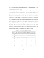
[9]). This property is of particular interest because storing the atom structure requires exponentially less space than the entire algebra. An example of this reduction
is given in Table 1.1. The first column represents the number of atoms of the relation algebra. The second column represents the size of the composition table, which
contains the largest portion of data needed to store relation algebra. Finally, the last
column represents the size of the composition table reduced to atoms.
Table 1.1: Space Compare: Algebra vs. Atom
Atoms in RA
The composition table size
Reduced to atoms size
1
4
1
2
16
4
3
64
9
4
256
16
5
1024
25
n
2n x 2n
nxn
2
In addition to reduction above it can be shown that considering so-called integral
algebras is sufficient. In fact, every relation algebra is equivalent to a matrix algebra
over a basis built from integral algebras [14, 15].
1.2
Goals
In this thesis I want to introduce and implement three structures representing atom
structures of integral heterogeneous relation algebras, i.e., categorical versions of relation algebras. As already mentioned above those algebras are sufficient to generate
all finite heterogeneous relation algebras. The first structure will simply embed a homogeneous atom structure of a relation algebra into the heterogeneous context. The
second structure is obtained by splitting all symmetric idempotent relations. This
new algebra is in almost all cases an heterogeneous structure having more objects
than the original one. Finally, I will define two different union operations to combine
two algebras into a single one.
1.3
Outline
Now, we outline the contents of the subsequent chapters.
Chapter 2: presents the necessary background required for the thesis, including an
introduction of heterogeneous relation algebras, and an overview of homogeneous relation algebras.
Chapter 3: describes three methods of generating finite integral heterogeneous relation algebras.
3
Chapter 4: presents a system which has implemented those three methods designed
in the previous chapter.
Chapter 5: offers a detailed user manual for the system.
Chapter 6: contains some concluding remarks, and some ideas about future work.
Parts of the thesis have been published in a conference [17]. In this paper the three
structures for
gen~rating
finite integral relation algebras as described in Chapter 3
are introduced. In addition the implementation which is presented in Chapter 4.3
was outlined.
4
Chapter 2
Background
Relation algebras have been studied since the latter half of the nineteenth century.
De Morgan (1864) and Peirce (1870) first founded the calculus of binary relations.
Schroder (1890 - 1905) carried on with their work. More than forty years later, Tarski
(1941) gave a first formal introduction to relation algebras. For more information,
see [9].
Originally, the theory of relations is homogeneous, i.e., every relation is considered
to be defined on a single and fixed universe U. In recent years a variant of this
theory based on category theory was developed in order to include relations with
different source and target. These approaches can be called heterogenous. Unlike the
homogeneous relation algebras, relations act between different sets in heterogeneous
relation algebras, e.g., the relation 'is-Illarried_to' which is a relation between the two
different sets of men and women. A classical (homogeneous) relation algebra can be
seen as a heterogeneous relation algebra with just one object (or single universe).
We have attempted to keep our notation and conventions in agreement with those
5
of the closely related subject of relation algebras, especially as presented in Maddux's
Relation Algebras [9j. We assume that the reader is familiar with the basic notions
from set theory and the theory of lattices.
In this chapter, first we will introduce the basic concepts of Boolean algebras and
category theory. Secondly, we will introduce heterogeneous relation algebras. Last,
we will review some fundamentals on (homogeneous) relation algebras.
2.1
Boolean Algebras
Since a relation algebra is based on a Boolean algebra, it is useful to review some
basic properties of Boolean algebras as well. For further reference see [3, 7, 9j.
Definition 1. An algebraic structure of the form Q3
and
=
(B, U, -) where U is a binary
is a unary operation is called a Boolean algebra if and only if it satisfies the
following three axioms (for all x, y, z E B):
1. xUy=yUx.
2. xU(yUz)=(xUy)Uz.
3. xUYUxUy=x.
The operation U is called union, and the operation
is called complementation.
In addition to the union (U) and complementation (-) operation of a Boolean
algebra one may define intersection (n) by x n y = xU y. Furthermore, there are two
constants, the zero or empty element 0 and the one or universal element 1, which
are defined by 0 = x n x and 1 = x U x for an arbitrary x E B, respectively. A
6
~
Boolean algebra is also equipped with a partial order defined by: x
if x U y
=
y. Notice that the property xU y
=
y if and only
y is equivalent to x n y
=
x. The
element xU y is the greatest lower bound of x and y with respect to the order
~,
i.e.,
xU y ~ x and xU y ~ y and whenever z ~ x and z ~ y, then xU y ~ z. Analogously,
,
x n y is the least upper bound of x and y. The concept of a greatest lower and a
least upper bound extends to any finite subset of B by iterating the operations
n, respectively. A Boolean algebra
~
U
and
is called complete iffl every subset of B has a
greatest lower and a least upper bound. Not every Boolean algebra is complete. For
an example we refer to [3, 7].
Any Boolean algebra is a distributive lattice, i.e., the equations x n (y U z)
(x
n y) U (x n z)
and xU (y
nz)
= (x U
y)
n (x u z)
hold for all x, y and z.
The powerset P(A) of a set A is an example of a Boolean algebra. The operation
(U) and the operation ( ) are given by union and complementation (relative to the
set A) of sets.
Definition 2. An element x of ~ is called an atom of ~ iff x
nonzero element of
At(~)
~
= {x I x =f o,x
is below x. We denote by
At~
i=
0 and there is no
the set of atoms
E ~ and Vy(y E ~,y ~ x =? Y = x or y
of~,
i.e.,
= O)}.
For example, when B is the Boolean algebra with two elements 0 and 1 with 0
~
1,
then 1 is the only atom in the algebra. The singleton sets are the atoms in the power
set. There are also Boolean algebras that contain no atoms but we will not consider
these algebras throughout this thesis.
Definition 3. A Boolean algebra is atomic if for every element x
IThroughout this thesis we will use 'iff' as a shorthand for 'if and only if'.
7
=f
0 there is an
atom a with a !;;;; x.
In particular every finite Boolean algebra is atomic. As already mentioned above
there are also non-atomic Boolean algebras but since we are mainly interested in finite
algebras we will only consider atomic ones.
In order to compare two different Boolean algebras the notion of a homomorphism,
i.e., a function preserving the structure of Boolean algebras, is of particular interest.
f
between two Boolean algebras
~l
and
function which preserves the Boolean operations, i.e., for all x, Y E
~l
we have
Definition 4. A homomorphism
~2
is a
1. f(x U y) = f(x) U f(y),
2. f(x) = f(x).
If it is possible to obtain a Boolean algebra from a given one by simply renaming
the elements, we consider the two algebras as being essentially the same, i.e., they
are isomorphic.
Definition 5. A homomorphism
a bijective homomorphism.
from
~l
to
~l
f : ~l
and
~2
---t ~2
is called an isomorphism iff it is
are isomorphic iff there is an isomorphism
~2.
For example, if Al = {Xl , ... ,xn }, A2 = {YI, '" ,Yn} are two sets, then there is a
bijective function j : Al
---t
A2 defined by j(Xi)
can be extended to an isomorphism k : P(A 1 )
P(At} and P(A 2 ) by k(B) = {j(x)
IX
E B}.
8
=
Yi for all! :::; i :::; n. This function j
---t
P(A 2 ) between the Boolean algebras
2.2
Category Theory
Later in Chapter 2.3, we will introduce a variant form of relation algebras whose
definition is based on category theory. In this variant of the theory relations are
heterogeneous, i.e., they may have different source and target such as the relation
'is_married_to' already mentioned at the beginning of this chapter.
Definition 6. A category C consists of the following two collections:
1. A class of objects Objcj
2. A class of morphisms Morc. Each morphism f has a source object A and a
target object B, which is usually indicated by the notation
f :A
--t
B. The
collection of all morphisms with source A and target B is denoted by C[A, B].
C is called locally small if C[A, B] is a set for every pair of objects A and B.
In addition, a category has a binary operation which is called composition (;). Composition is defined for each pair of morphisms
a morphism, f; g : A
--t
f :A
--t
Band g : B
--t
C, and yields
C. The following axioms are valid:
Identity: For every object A, there is a morphism ITA, called the identity morphism
for A, such that for every morphism f : A
Associativity: For all f : A
--t
B, g : B
--t
--t
B, we have f; ITA = IT B ; f = f·
C, and h : C
--t
D, we have f; (g; h)
=
(j; g); h.
In the definition above composition of morphisms has to be read from left to right,
i.e., f; g means first f, then g.
Below we have listed some typical examples of concrete categories:
9
Set: The category with sets as objects and functions as morphisms.
Vee: The category with vector spaces as objects and linear maps as morphisms.
Top: The category with topological spaces as objects and continuous functions as
morphisms.
There are also examples of categories that are not based on functions between
some (structured) sets. For instance, any ordered set is a category, where the objects
are elements of the set and there is exactly one morphism with source x and target
y iff x ::; y. The axioms of a category are satisfied because the reflexivity of the
order induces the identity morphisms and its transitivity implies the associativity of
composition.
A homomorphism between categories is called a functor.
Definition 7. Let C1 and C2 be categories. A functor F : C1
operations
FObj :
Objcl
-+
Objc2' F'Mor : Morcl
-+
FObj(B)
-+
-+
C2 is a pair of
Morc2 such that for each f : A
-+
B,g:B-+CinC1 ,
• FMor(f) : FObj(A)
• FMor(f; g) = FMor(f); FMor(g)
A functor F is called full if for all A, BE Objcl and every i E C2 [F(A), F(B)] there
is fECI [A, B] such that i = F(f).
F is called faithful if for all A , B E Objcl and for all f, h E CdA, BJ, F(f) =
F(h) implies f
=
h.
10
In category theory the weaker notion of equivalent categories is usually used instead of the stronger notion of isomorphism. However, since we are mainly interested
in finite structures we will use the stronger concept of isomorphism.
Definition 8. A functor is called an isomorphism iff it is full, faithful and bijective
on objects. Two categories C1 and C2 are isomorphic if there exists an isomorphism
F: C1
~
C2 •
Two isomorphic categories share all properties that are defined in terms of category
theory.
2.3
Heterogeneous Relation Algebras
In this section we recall some fundamentals on heterogeneous relation algebras. For
further details we refer to [5, 11, 10].
Definition 9. A heterogeneous relation algebra is a locally small category R. Its
morphisms are usually called relations. In addition, there is a unary operation
R[A, B]
---t
~B
:
R[B, A] between the sets of morphisms, called conversion. The opera-
tions satisfy the following rules:
1. Every set R[A, B] carries the structure of a complete atomic Boolean algebra
with operations UAB, nAB, - AB, zero elementJLAB, universal elementlrAB, and
inclusion ordering
~AB'
2. The Schroder equivalences
Q; R ~AC S
<=>
Q ~; S ~BC R
11
<=> S; R~
~AB Q
hold for relations Q : A
-t
B, R: B
-t
C, and S : A
-t
C.
The definition of heterogeneous relation algebras is based on category theory. All
the indices of elements and operations are usually omitted for brevity and can easily
be reinvented.
Let ReI be the relation algebra which has sets as objects and concrete binary
relations as morphisms. A concrete binary relation R between A and B is a set of
pairs from A and B, i.e., R
~
A x B where A x B is the cartesian product of the
sets A and B . In the remainder of this thesis we will also write xQy for (x, y) E Q.
Suppose Q, S
Converse:
~
Q~
A x Band R
= {(y,x)
E
~
B x C. Then the operations are defined as follows:
B x A I xQy},
Complement: Q = {(x, y) E A x B I (x , y)
rf. Q},
Union: Q U S = {(x, y) E A x B I xQy or xSy},
Intersection: Q n S = {(x, y) E A x B I xQy and xSy} ,
Composition: Q; R = {(x, z) E A x C I (:3y E B) xQy and yRz}.
The following is an example of a composition in the heterogenous relation algebra
Rel.
Suppose A = {I, 2, 3} , B = {a , b, c}, C = {True , False} are objects in ReI, and
Q
= {(I, True), (2, True), (3 , False)},S
=
{(False , a), (False, b), (True,c)}, T
{(I , c), (2, c), (3, a), (3, b)} are relations with Q : A
-t
C, S: C
-t
Band T : A
-t
=
B.
Relations in ReI can alternatively be represented by Boolean matrices. For example, the first matrix below represents Q in the following sense. The three rows
12
represent the three elements in A, and the two columns the two elements in C.
Therefore, the 1 in the upper left corner indicates that the first element of A, the
element 1, is in relation Q with the first element of C, the element True. Analogously,
the 0 in the lower left corner indicates that (3, True) ¢ Q.
,
Then
1 0
Q;8=
1 0
;
(:
0 0 1
0
1
0 1
Lemma 1. Given relations R : A
P :A
-t
-t
:)
B, Q : A
0 0 1
=T
1 1 0
-t
B, 8 : B
-t
C, T : B
-t
C,
C, then we have:
(a) R; (8 n T)
r;;, R; 8 n R; T
(b) R;8npr;;,R;(8nR~;p) andR;8npr;;,(Rnp;8~);8
(c) R; (8 U T)
= R; 8 U R; T
(d) (R; 8)~ =
8~; R~
The proof of this lemma can be found in either of [9, 10, 11].
Since a heterogeneous relation algebra is a locally small category, where every
hom-set is a Boolean algebra, we define homomorphisms between relation algebras
based on functors and homomorphisms of Boolean algebras.
Definition 10. A homomorphism between two relation algebras Rl and R2 is a
functor F : Rl
-t
R2 so that the function induced by F between Rl [A, B] and
13
R 2[F(A), F(B)] is a homomorphism between Boolean algebras for every pair of objects
A and B .
Definition 11. A homomorphism F : Rl
--7
'R2 is called an isomorphism iff it is
full" faithful and bijective on objects. Two relation algebras Rl and R2 are isomorphic
(Rl
~ R 2), iff there is an isomorphism from
Notice that if F : Rl
--7
Rl to'R 2.
R2 is an isomorphism between relation algebras, then the
induced function between R1[A, B] to R 2[F(A), F(B)] is an isomorphism between
Boolean algebras for every pair of objects A and B .
2.3.1
Integral Object
Integral objects are of particular interest since it can be shown that certain heterogenous relation algebras are equivalent to matrix algebras with coefficients given by
relations between integral objects. For further detail see [14].
Following the notion used in algebra, we call an object A integral if there are no
zero divisors within the subalgebra R[A, A]. Later on, the class of integral objects
will define the basis of R.
Definition 12. An object A of a relation algebra is called integral iff JLAA
for all Q, R E R[A, A] the equation Q; R
-I-lrAA
and
= JLAA implies either Q = JLAA or R = JLA A .
The following example shows that not all objects are integral.
Let A = {1,2} be an object of ReI, and Q
R[A,A].
14
= {(I, I)} , S = {(2, I)} be relations in
Then
However, neither Q = JL nor S = JL, i.e., the object A is not integral. Actually,
the integral objects in ReI are the singleton sets.
It can be shown [14, 15] that the property of being integral is equivalent to the
properties 'llA is an atom' or 'every relation not equal JLAA is total'.
The basis Bn of R is defined as the full subcategory given by the class of all
integral objects.
2.3.2
Symmetric Idempotent Relation
The notion of a splitting combines subobjects (or subsets) and the set of equivalence
cla..')ses of an equivalence relation into one concept [5]. In order to define this concept
we first need the notion of a partial equivalence or a symmetric idempotent relation.
Definition 13. A relation X : A
X~ =
X and X; X
=
-t
A is called a symmetric idempotent relation, iff
X.
Suppose A = {Peter, Jon, Mary, Paul, Carly, Anna, Debbie, Dave} is a set of persons and an object in ReI. Let X : A
--1
A be the relation on this set of persons that re-
lates two persons if they went to the same country for vacation this year. We have X
=
{(Peter, Peter), (Peter, Mary), (Peter, Paul), (Jon, Jon), (Mary, Peter), (Mary, Mary),
(Mary, Paul), (Paul, Peter), (Paul, Mary), (Paul, Paul), (Anna, Debbie), (Anna, Anna),
15
(Debbie, Debbie), (Debbie, Anna)} or as a Boolean matrix:
Carly Anna Debbie Dave
Peter
Jon
Mary
Paul
Peter
1
0
1
1
0
0
0
0
Jon
0
1
0
0
0
0
0
0
Mary
1
0
1
1
0
0
0
0
Paul
1
0
1
1
0
0
0
0
Carly
0
0
0
0
0
0
0
0
Anna
0
0
0
0
0
1
1
0
Debbie
0
0
0
0
0
1
1
0
Dave
0
0
0
0
0
0
0
0
Notice that Carly and Dave did not go on vacation this year so that they are not in
relation to themselves. X is a partial equivalence relation that has three equivalence
classes - the sets {Peter, Mary, Paul}, {Jon} and {Anna, Debbie} - and two elements
that do not belong to any equivalence class - the elements Carly and Dave.
Some basic properties of symmetric idempotent relations needed throughout the
thesis are listed in the following lemma.
Lemma 2. If X : A
---7
A and Y : B
---7
B are symmetric idempotent relations, then
(a) X;(QnR);Y=X;Q;YnX;R;Y JorallQ,R:A---7B withX;Q;YJ;;;;Q,
(b) X;X;Q;Y;Y J;;;; Q Jar all Q: A
(c) Q J;;;; X; Q; Y or all Q : A
---7
---7
B,
B with X; Q; Y
(d) X;X;Q;Y;Y = Q for all Q: A
---7
~
Q,
B with X;Q;Y = Q.
16
Proof. (a) We have X; (Q
n R); Y !;;:; X; Q; Y n X; R; Y
Lemma 1 (a)
For the converse inclusion we have
X;Q;Y nX;R;Y!;;:; X; (X~;X;Q;Y n R;Y)
X~=X
=x;(X;Q;YnR;Y)
!;;:; X; (X; Q; Y; Y~
Lemma 1 (b)
n R); Y
andX;X=X
Lemma 1 (b)
=X;(X;Q;YnR);Y
Y~=YandY;Y=Y
!;;:;X;(QnR);Y
X;Q;Y!;;:;Q
(b) The assumption follows from
X'Q'Y
, , C- X'Q'Y
, ,
{:}
X'Q'Y'Y~
C
"
-
,
Schroder equivalences
X'Q
,
Y~=Y
{:} X;Q;Y;Y!;;:; X;Q
{:} X'Q
, -C X'Q'Y'Y
, , ,
{:}
, X'Q'Y'Y
, , ,
X~·
Schroder equivalences
C
- Q
{:}X'X'Q'Y'YCQ
, , , , -
X~=X
17
(c) We have
Assumption
X;Q;Y!;;;;;Q
{:}
Q;Y~!;;;;;
X;Q
Schroder equivalences
{:}Q;Y!;;;;;X;Q
{:}X;Q!;;;;;Q;Y
{:}X~;Q;Y!;;;;;Q
Schroder equivalences
{:} X;Q;Y!;;;;; Q
X~=X
{:} Q!;;;;; X;Q;Y
(d) From (b) , we obtain the inclusion!;;;;; . The converse inclusion follows from Q =
o
X;Q;Y!;;;;; X;X; Q;Y; Y using (c).
Now, we are ready to define the concept of a splitting.
Definition 14. Let
n
be a relation algebra, and X : A
-t
A be a symmetric idem-
potent relation. Then an object B together with a relation R : B
splitting of X iff R; R~
-t
A is called a
= IB and R~; R = X.
Consider again the set A of persons and the symmetric and idempotent relation
X : A
-t
A from above. The object B of the splitting of X is the set of the
equivalence classes, Le., it is the set containing the three sets {Peter, Mary, Paul},
{Jon} and {Anna, Debbie}. The splitting R : B
18
-t
A is the relation that relates
every equivalence class to its elements, i.e., it is given by R
=
Peter
Jon
Mary
Paul
Carly
Anna
Debbie
Dave
{Peter, Mary, Paul}
1
0
1
1
0
0
0
0
{Jon}
0
1
0
0
0
0
0
0
{Anna, Debbie}
0
0
0
0
0
1
1
0
Theorem 1. Every relation algebra can be faithfully embedded into an algebra that
provides all splittings.
Proof. Let n be a relation algebra, and define a relation algebra n+ as follows. The
class of object Obh.+ is the class of all SID (symmetric idempotent relations) from
n.
Given two SID X : A ---+ A and Y : B ---+ B, the set of relations between X and
Y in n+ is defined by n+[X, Y] = {R : A ---+ B
I X; R; Y
=
R}. All operations
except complement are inherited from n. The complement of S E n+[X, Y] is given
by X; S; Y. Therefore, given T , S E n+[X, YJ, Q E n+[Y, Z] and R E n+[X, Z] we
need to show:
1. X;T;Q; Z = T;Q,
2. X ; (TnS);Y=TnS,
3. X;(TUS);Y=TUS,
4. The operation U together with the complement X; S; Y for S E n+ [X, Y] forms
a Boolean algebra, i.e., we have X; X; Q; Y U X; R; Y; Y U X; X; Q; Y U R; Y
Q for all Q, R
E n+[X, Y].
19
=
6. lIx =X,
7. The Schroder equivalences are valid, i.e.,
We now show each of Equations 1-7 above:
1. Suppose T E n+[X, Y] and Q E n+[Y, Z]. Then we have
X'T'Q'Z=X'X'T'Y'Y'Q'Z'Z
,
""'"
"
, , and Q = Y'Q'Z
, ,
T = X·T·Y
, , , , ,
=X'T'Y'Y'Q'Z
x
=T;Q
, , = T and Y'Q'
, ,Z = Q
X'T'Y
= X; X and Z = Z; Z
2. Suppose T, S E n+[X, Y]. Then we have
X;(TnS);Y=X;T;YnX;S;Y
= Tn S
Lemma 2 (a)
T = X; T; Y and S = X; S; Y
TnS=X;T;YnS
T=X;T;Y
~
X; (T; Y n X~; S)
Lemma 1 (b)
~
X; (T n X~; S; Y~); Y
Lemma 1 (b)
=X;(TnX;S;Y);Y
X=X~andY=Y~
=X;(TnS);Y
S=X;S;Y
20
3. Suppose T, S E R+[X, Y]. Then we have
X·, (T U S)·, Y
(X·,TuX ·" S)· Y
Lemma 1 (c)
= X;T;YUX;S;Y
Lemma 1 (c)
=TuS
T=X;T;YandS=X;S;Y
=
4. X;X;Q;YUX;R;Y;YUX;X;Q;YuR;Y
Definition of
= X· (x·Q·YnX·R·Y)·YUX· (X·Q·YnR)·Y
, "
'"
'"
,
n
= (X;X;Q;Y;Y nX;X;R;Y;Y) U (X;X;Q;Y;Y nX;R;Y) Lemma 2 (a)
= (QnR) U (QnX;R;Y)
Lemma 2 (d)
= Q n (R U X; R; Y)
Definition of U
= Q n (X;R;Y UX;R;Y)
Lemma 1 (c)
=QnX;(RUR);Y
= X;Q;Y nX; (RU R);Y
= X;
Lemma 2 (a)
(Q n (RU R));Y
=X;Q;Y
=Q
5. Suppose S E R+[X, Y]. Then we have
X
=X;S;Y~
=
X~
and Y =
Lemma 1 (d)
21
Y~
6. Suppose 8 E n+[X, Y]. We have to show that X; 8 = 8 for all 8 E n+[X, Y]
and T;X = T for all T E n+[z, X].
X;8=X;X;8;Y
7. 8;Q
~
8=X;8;Y
=X;8;Y
X=X;X
=8
X;8;Y=8
R
Schroder equivalences
::::} y., 8~', R-, Z -C y., Q', Z
{:} y., y ,. 8~', X·, R-, Z C
- y., Q', Z
{:}
Y;8~;X;X;R;Z ~
{:}
8~'
, X·, R-, Z C-
Y;Q;Z
y., Q', Z
(5)
Y; Y = Y and X; X
=X
(5)
The converse implication is shown by
C y.Q.
, , R-Z·
, ,, ,Z
8~'X'
{:}8'Y'Q'ZCX'R-Z
, , , - , ,
Schroder equivalences
::::} X'8'Y
, , ', Q'Z'
, ,Z C
- X·, X·, R-Z'Z
, ,
{:} X;X;8;Y;Y;Q;Z;Z
~
X;X;R;Z;Z
X;8;Y
=
8
{:} X;8;Y;Y;Y;Q;Z;Z ~ X;X ; R;Z;Z
XiX = X and Y;Y = Y
{:} X; 8; Y ; Q ~ R
Lemma 2 (d)
{:}8;Q~R
X;8;Y=8
The second equivalence is shown analogously.
22
We have just shown that R+ is a relation algebra, which inherits all operations
from R. The next thing we have to prove is that R can be faithfully embedded into
R+.
Define a functor F : R
F(T)
--t
R+ by F(A) = ITA for every object A in R, and
= T for every relation. This functor is obviously full and faithful.
The last thing we have to show is that R+ provides all splittings. Let U be SID
in R+, where U : X
X; U; X
X. By definition we know that U~
--t
= U, U; U = U and
= U Therefore U is also an object in R+. Furthermore, we have
U;U;X = U;X
U;U=U
=X;U;X;X
U=X;U;X
=X;U;X
X;X=X
=U
X;U;X=U
i.e., U E R+[U,X]. From
U;
U~
= U = ITu and
U~;
U
=U
We conclude that the object U and the relation U E R+ [U, X] is a splitting of
U E R+[X,X].
0
Later, in Chapter 3, we will use the concept of symmetric idempotent relations to
define one structure that represents atom structures of heterogenous relation algebras.
Definition 15. Given two relation algebras Rl and R 2 , define their direct sum
Rl +0 R2 as follows:
• The class of object
Obj(Rl+oR2)
is the union of all objects from Rl and R 2 •
23
• The set of relations between objects A and B is defined by:
'R.dA, B], A, B
('R.1 +0 'R. 2 )[A, B]
E
Obj'R1
'R. 2 [A, BJ, A, B E Obj'R2
=
otherwise .
• For Q : A
~
B, S: B
~
C, the composition (;) is defined by:
Q;S,
Q;8=
{ JL ,
AC
otherwise.
Theorem 2. The directed sum of two relation algebras is also a relation algebra, and
the given relation algebras can be embedded into it.
Proof. Since 'R. 1 and 'R. 2 are relation algebras, and JL is the only element between
objects of different inner relation algebras, each set ('R. 1 +0 'R. 2 ) [A, B] is a Boolean
algebra.
For each triple of morphisms T E ('R. 1
+0
'R. 2 )[A, BJ, 8 E ('R. 1
+0
'R. 2 )[B, C] and
Q E ('R. 1 +0 'R. 2 )[C, D]; the associativity (T; 8); Q = T; (8; Q) holds if A, B, C, Dare
all either from 'R. 1 or'R.2 . Otherwise one of the relations T,8 or Q equals JL Assume
T = JLAB , then we have
(T; 8); Q
=
(JLAB; 8); Q
T; (8; Q) =JLAB ; (8; Q)
24
The other cases are similar.
Therefore (T; 8); Q = T; (8; Q), and the associativity is valid.
If all relations are in one of the relation algebras R1 or R 2, the Schroder equiva-
lences are vaild. Otherwise assume T E (R1 +0 R 2)[X, Yl, 8 E (R1 +0 R 2)[X, Zl and
.
T;Q
= T;JLyz
the definition of composition
=JLxz
[;;;xz
+0 R 2) [X, Zl
8 E (R1
+0 R 2) [X, Z]
the definition of composition
=JLyZ
[;;;YZ
E (R1
8
8
Q
Therefore T; Q [;;;xz 8 {:} T~; S
[;;;YZ
Q. The other equivalences are shown analo-
gously.
R1 and R2 are embedded into (R1
+0 R 2) because the class of object Obj('Rl+o'R2)
is the union of all objects from R1 and R 2.
o
In the case of integral relation algebras the directed sum can be enlarged by using
a two-element Boolean algebra instead of the trivial one-element Boolean algebra as
the intermediate morphism sets.
Definition 16. Given two integral relation algebras R1 and R21 define their en-
larged sum R1 +1 R2 as follows:
• The class of object Obj('Rl+l'R2) is the union of all objects from R1 and R 2.
25
• The set of relations between objects A and B is defined by:
(R1 +1 R 2 )[A, B]
• For Q : A
---t
B, S: B
---t
=
R 1 [A, B],
A,B
R 2 [A, B],
A,B E Objn2
E
Objnl
C, the composition (;) is defined by:
Q; S, A, B, C E Objnl or A, B, C E Objn2
Q; S
=
= JLAB
JLAC ,
Q
T AC ,
otherwise
or S
= JLBc
Theorem 3. The enlarged sum of two integral relation algebras is also a relation
algebra, and the given relation algebras can be embedded into it.
Proof. The proof of this theorem is very similar to the proof of Theorem 2. Therefore,
we just show the Schroder equivalences as an example.
Suppose T E (R1 +1 R 2 )[X, Y], S E (R1 +1 R 2 )[X, Zj and Q E (R1 +1 R 2 )[Y, Z],
where X, Y E Obk1 and Z E Objn2'
If Q =JLyZ, then we obtain
T;Q
= T;JLyz
the definition of composition
=JLxz
I;;:xz
S E (R1 +1 R 2 )[X,Zj
S
Lemma 1 (b)
= T'~;JLxz
T;Q !;xz S
=JLyZ
the definition of composition
26
If T
=
JLXY , then
T;Q =JLXy;Q
the definition of composition
=JLxz
[;;;xz S
T~; S =JLyX ; S
the definition of composition
=JLyZ
Otherwise we get
T;Q
T~; S
= T;lryz
=lrxz
the definition of composition
[;;;xz S
S E (R1 +1 R 2) [X, Z]
= T~;lrxz
S E (R1 +1 R 2) [X, Z]
=lryZ
the definition of composition
[;;;YZ
Therefore T; Q [;;;xz S
Q
{?
T~; S
[;;;YZ
Q. The other equivalences are shown analo-
~~
D
Another way of constructing a relation algebra from given ones is to consider pairs
of relations.
Definition 17. Given two relation algebras R1 and R 2, their product R1 x R2 is
defined by:
• The class of object Obj(1'-lX'R2) = {(A,B)IA E Obj'R1,B E Obj'R2}
27
• The set of relations in R1 x R2 is a set of pairs, the first element is a relation
from R1 and the second element is a relation from R 2.
• The composition is inherited from R1 and R2 and applied componentwise.
Theorem 4. The product of two relation algebras is also a relation algebra.
Proof. Given two relation algebras R1 and R 2, and we define the product of two
relation algebras R1 x R2 by following its definition. The set of relations in R1 x R2
carries the structure of a complete atomic Boolean algebra.
For each set of morphisms in R1 x R 2, we need to show the associativity. Let
Q1 : Xl
---->
Yl,8 1 : Y1
Q2 : X 2 ----> Y2, 8 2 : Y2
---->
---->
Zl, and T1 : Zl
Z2, and T2 : Z2
(Q1, Q2); ((81 ,82 ); (T1' T2))
---->
Xl, where Xl, Yl, Zl E ObjRl; and
---->
X 2, where X 2, 12, Z2
=
(Q1, Q2); (81 ; T 1, 8 2 ; T 2)
=
(Q1; 8 1 ; T 1, Q2; 8 2 ; T2)
E
Obj R2·
((Ql, Q2); (81 ,82 )); (T1' T2) = (Q1; 8 1 , Q2; 8 2 ); (T1' T 2)
Therefore (Q1, Q2); ((81 ,82 ); (Tl, T2))
=
(Q1; 8 1 ; T 1, Q2; 8 2 ; T2)
=
((Q1, Q2); (81 ,82 )); (T1' T2)
Now we need to show the Schroder equivalences.
(Q1, Q2); (81 , 8 2 ) ~ (T1' T2) {:} (Q1; 8 1 , Q2; 8 2 ) ~ (T1' T 2)
{:} Q1; 8 1
{:}
~
T1 and Q2; 8 2
Q1~;81 ~
The other equivalences follow analogously.
28
T1 and
~
T2
Q2~;82 ~
T2
o
2.4
Homogeneous Relation Algebras
In this section we review the basic concepts of homogeneous relation algebras. For
further details we refer to [9, 4]. A homogeneous relation algebra is a heterogenous
relation algebra with one object.
2.4.1
Atom Structure
Every relation algebra provides an atom structure, i.e., a relational structure on its
set of atoms. For further details not mentioned in this chapter we refer to [8].
The operations of the underlying Boolean algebra correspond to the set-theoretic
operations of union, intersection and complement on sets of atoms. Some additional
structure on atoms is needed to recover composition and converse of the relations.
Notice that the converse of an atom is an atom again. For a proof see [8].
Definition 18. Let R be a finite homogenous relation algebra. The atom structure
ofR is a structure of form Q(.t(R) = (At(R),C,~,I), where At(R) is the set of
atoms ofR, C = {(x,y,z) : z ~ x;y} is a ternary relation on At(R), i.e., C ~
At(R) x At(R) x At(R) and I = {x : x E At(R) , x ~ lI}.
We need to prove the following theorem in order to define the concept of a cycle.
This concept can be used to represent the ternary relation C in a more compact
manner.
Theorem 5. Let Q(.t(R) be the atom structure of a finite homogeneous relation algebra.
Then (x, y, z) E C iff (x, z, y) E C iff (y, '1, x) E C iff (V, x, '1) E C iff ('1, x, V) E C iff
(z,V,x) E C.
29
Proof. (x, y, Z) E C
{:} Z ~
{:} z
x; y
n x; y of- 0
{:} x;y g
z is an atom.
z
Boolean algebra property.
Schroder equivalences.
Boolean algebra property.
y is an atom.
(x~,z,y) E
C
o
All other implications are shown analogously.
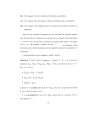
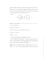
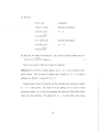
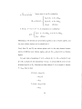
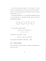
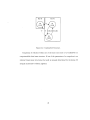
Due to the theorem, we define a cycle [x,y,z] by
[x, y, z] = {(x, y, z), (y, z, x), (z, 1), x)(x, z, y), (1), x, z), (z, x, 1))}
A cycle can nicely be visualized by the following diagrams.
x
z
1\z•
y
1\£
z.II
x
1'\
..
y-
Figure 2.1: Cycle law for binary relations.
30
If one of the directed triangles in Figure 2.1 is in the relation C of an atom
structure of a relation algebra, then so are the others. In other words, the relation C
is the union of certain cycles. Furthermore, it is sufficient to store only one element
as the representative of a cycle.
For an example consider the set A
=
{I, 2} and the relation algebra R with object
A and all binary relations on A. Represented as Boolean matrices, the atoms of R
are the following four relations:
The atom structure is, therefore, given by
At(~) =
Ii
{a,b,e,d}, and
=
a,
b=
I(~) =
e, C= b,
d=
{a,d}.
d.
By the definition of cycle structures, we obtain
C(~)
= {[a, a, a], [b, e, a], [e, b, d], [d, d, d]}.
The atom structure of ~ is QH(~) = (At(~), C(~),
2.4.2
~,I(~)).
Complex Algebra
We are now interested in the converse process, i.e., defining a relation algebra if an
atom structure is given.
31
Definition 19. Let be 6 = (U, C, f, J) a relational structure such that C
~
UxUx
U, f : U --+ U and J ~ U. The complex algebra of6 is ctm(6) = (P(U), U, -,;, ~,J),
where X; Y
=
{z : (:3x E X)(:3y E Y)( (x, y, z) E C)}, and
any subset X, Y
.
~
X~ =
{Jx : x E X}, for
U.
We continue with the example which was given in the previous section. In this
case, the given relational structure is 6 =
Q(t(~)
=
(At(~), C(~),
~,J(~)).
A finite relation algebra is completely determined by the action of composition on
its atoms. The cycles completely determine the composition operation.
Let X = {a, b}, Y = {c, d}, we have {a, b}; {c, d} = {a, b} by the definition of the
relation C(B). This corresponds to the composition of the following two matrices in
the original algebra.
By the definition of the relation C(B), and
{a,b}~ =
{Ja,fb}
=
{a,c}. This
corresponds to the union of the following two matrices in the original algebra.
(: :) u (::)
(::)
The connections between atom structures and complex algebras have been presented in [8] as following: If Q( is a complete and atomic relation algebra, then
Q(
~
and
ctm(Q(t(Q()). Furthermore, any two complete and atomic relation algebras Q(
~,
Q(
~ ~
iff Q(t(Q()
~ 5.2(t(~).
32
It is well-known that every atomic relation algebra induces a particular structure
on its atoms: its atom structure. In particular, composition is represented by a set of
triples of atoms, i.e., by a ternary relation. Conversely, given an atom structure one
may form the complex algebra thereof. The structure obtained is, in general, neither
integral nor a relation algebra.
Following properties in [9] characterize the atom structure that lead to a relation
algebra.
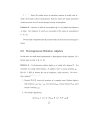
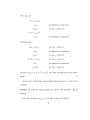
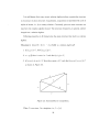
Theorem 6. Given Qt
=
(U, C,
~,
I), Itm(Qt) is a relation algebra iff
1. if (x, y, z) E C, then [x, y, z] ~ C.
2. x = y iff there is some i E I such that (x, i, y) E C,
3. if (v, w, x), (x, y, z) E C then there exists u E U such that (w, y, u), (v, u, z) E C
as shown in Figure 2.2.
u
v
Figure 2.2: Associativity for composition.
When I' is an atom, I is a singleton, i.e., I = {e}.
33
Theorem 7. Given Qt
(U,C,
=
~,{e}),
• Itm(Qt) is integral iffQt satisfies condition (a) .
• Itm(Qt) is a relation algebra, iff Qt satisfies conditions (a) and (b).
(a) if x
=1=
y then there is some w E U
(b) if (v,w,x), (x,y,z)
E
C and v
=1=
rv
z,
{e} such that (x, w, y) E C .
w =1=
y then there exists u E U
rv
{e} such
that (w,y,u), (v,u,z) E C.
Later, in Chapter 4, we will use these properties to check whether the complex
algebra of a given relational structure on a set is a relation algebra .
34
Chapter 3
Three Structures representing
Relation Algebras
In this chapter we want to introduce three structures representing atom structures
of integral heterogenous relation algebras. The first structure simply embeds a homogeneous atom structure into the heterogenous context. The second structure is
obtained by splitting all symmetric idempotent relations. Finally, we define a structure representing the direct and the enlarged sum of two algebras.
3.1
The Structure HomNA
In this section we define the structure HornN A. Recall that this structure resembles
the atom structure of a relation algebra. The abbreviation NA stands for nonassociative. If condition (b) of Theorem 7 is not satisfied, then the composition in the
complex algebra is not associative, and hence, the use of this name.
The following structures and operations were implemented in the programming
35
language Haskell. Therefore, we present the structures in a Haskell-pseudocode, i.e.,
using constructors and tuple notation to represent structures.
Definition 20. The structure RNA (name, n, s , i , eye, i sRA) is called a H omNA where
• n
is the number of atoms,
• s is the number of symmetric atoms, i.e., 1 :::; s :::; n,
• i is the index of the structure within all possible structures with n atoms and s
symmetric atoms,
• eye is the ternary relation for composition given by cycles (cf. [9]),
• isRA is true iff the structure is an integral relation algebra.
As a representation of the atoms we use natural numbers 1, . . . , n with the following conventions. The identity, which is an atom in an integral structure, will always
be atom 1. The atoms 1, ... , s are symmetric, and the remaining atoms s
are non-symmetric with
m~
= m + 1 if m - s is odd and
m~
+ 1, ... , n
= m - 1 if m - s is
even. Consequently, n - s must be even.
The Boolean part of the complex algebra of an HomNA is defined as usual, and
the converse operation on sets is defined componentwise. In the following we want
to briefly explain how to compute composition in the complex algebra. First of all,
the ternary relation eye is given by cycles [9J . Recall that a cycle is a triple of atoms
[x, y, zJ representing up to six triples, i.e.,
36
Furthermore, we omit the cycles involving the identity, i.e., the cycles [x, 1, xl for
every atom x. eye can now be computed as the union of the identity cycles and the
cycles of the structure.
We want to illustrate the whole concept by an example. Consider the HomNA
HNA (4,2,98, {[2, 2,2] , [2,2,3] , [3,3, 3J} , True). This structure has 4 atoms with
the following converse operation
1~ = 1,
2~
= 2,
3~
= 4, 4~ = 3.
Expanding the set of cycles we get
eye
= {(1,1,1),(2,1,2),(2,2,1),(1,2,2),(3,1,3),(4,3,1),(1,4,4),(4,1,4),
(3,4,1), (1,3,3),(2,2,2), (2,2,3), (2,3,2),(3,2,2),(2,2,4), (2,4,2),
(4,2,2),(3,3,3),(4,3,3),(3,4,3),(4,4,4),(3,4,4),(4,3,4)}.
Composition in the complex algebra is now defined by
X ;Y:= {zlx
E
X , y E Y,(x,y,z)
E eye}.
Now, consider the sets of atoms A = {2, 3} and B = {2}. Then we have
A~
3.2
=
{2~, 3~}
= {2, 4}, A; B = {2; 2} U{3; 2} = {1, 2, 3, 4}.
The Structure SplitN A
In this section we want to introduce the structure SplitNA. A SplitNA is generated by
splitting all symmetric idempotent relations of a HomNA. For each of the additional
objects of this category according to the embedding sketched in Section 3.1 a HomNA
37
is computed and stored in the new structure. In addition, for each heterogeneous homsets, i.e., the sets of relation with different source and target, the number of atoms is
computed. For each such number its extension, i.e., the original relation, is stored.
Definition 21. The structure SNA(root,objs,atoms) is called a SplitNA where
• root is a HomNA (the root of this structure),
• obj s is a set of HomNAs representing the objects,
• atoms is a function mapping hom-set to a list of relations of the root object.
Notice that in the actual implementation the elements of objs are in fact just
triples consisting of n, sand i. This information together with the enumeration
algorithm implemented is sufficient to identify the corresponding HomNA.
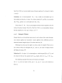
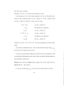
We illustrate this structure by an example. The whole SplitNA including the
function atoms is visualized in the Diagram 3.1:
.3}
Figure 3.1: The Structure SplitNA.
38
We start with the HomNA with n = 3, s = 1 and i = 1 as the root object. This algebra has exactly three symmetric and idempotent relations: the identity, the empty and the universal relation. The identity generates the original algeb~a
as an object of SplitNA. The other two relations generate HomNAs with
n = 0, s =
°
and i =
°
and n = 1, s = 1 and i = 0, respectively. Therefore objs
=
[(0,0,0), (3, 1, 1), (1, 1,0)] and we indicate each object by its index in objs. In this
case, atoms = [((0,0), [J),( (0,1), [J),( (0,2) ,[J), ((1,0) ,[J),( (1,1) ,[[1 J, [2],[3]]), ((1,2), [[1,2,3]]),
(( 2,0), [J), ((2,1), [[1 ,2,3]]), ((2,2), [[1 ,2,3]])].
For example, there are no atoms between the objects (0,0,0) (index 0) and (3 ,1,1)
(index 1). On the other hand, there is exactly one atom between (1,1,0) and itself.
This atom is the the union of the atom 1,2 and 3 of the original relation algebra, i.e,
the object (3,1,1).
3.3
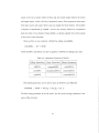
CombineNA Structure
In this section we introduce the structure CombineNA. This structure implements
the directed as well as the enlarged sum of two algebras as defined in Section 2.
Therefore, it consists of a list of inner NAs, i.e., each element is a HomNA, SplitNA
or CombineNA. Furthermore, it indicates whether the hom-sets between objects of
different inner NAs has
°
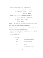
or 1 atom. The structure is visualized in Figure 3.2. In
this example there are two NAs. NA#O is a HomNA, and NA#l is a SplitNA. The
CombineNA was generated by specifying that there should be
°
atoms in the hom-sets
between objects of different inner NAs (dashed arrows). Le., that we use the direct
sum construction.
39
NA #1
NA #0
Figure 3.2: CombineNA Structure.
Composition of relations within one of the inner structures of a CombineNA is
computed within that inner structure. If one of the parameters of a composition is a
relation between inner structures, the result is uniquely determined by the axioms of
integral nonassociative relation algebras.
40
,
Chapter 4
Implementation
4.1
Overview
In this chapter, we present the implementation of our work. In general, the system
is capable of doing the following three tasks.
1. Compute all relation algebras with n atoms and s symmetric atoms. This works
using the tables on the disk. We first divide the table entries into two parts:
non-isomorphic NAs and isomorphic NAs. For isomorphic NAs entries, we just
need to check isRA property for the first element in the isomorphic list, and
the rest is filled automatically. Conversely, non-isomorphic NAs entries have to
check the i sRA property all the time.
2. Provide a user interface in which a user can design a basis using the three
structures from Chapter 3. During this process the structure, i.e., how the
basis is built, is kept.
41
3. Export a basis as a heterogeneous algebra suitable to be used by another program. The algebras are stored in XML. This format can be used by the ReAlM
system [1]. The additional information of how the basis was constructed is not
stored.
The system has been developed using the functional programming language Haskell.
A Haskell program consists of a collection of modules. A module defines a collection
of values, datatypes, type synonyms, classes, etc. We will discuss how each module
of the system relates to our work. Figure 4.1 shows the dependencies between the
modules of the system. The user interface has been developed by using GTK and
Figure 4.1: The Relationship of Modules.
the Haskell library Gtk2Hs. The graphic has been generated by Graphviz which is a
graph visualization software. Throughout this chapter we assume that the reader is
familiar with the language Haskell and its standard libraries.
42
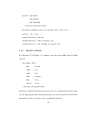
4.2
Atom Structure Module
The Atom Structure Module groups a set of related functionalities into a single
package and manages them. It exports some of these resources and makes them
available for other modules, e.g., HomNA, HetNA.
In Chapter 2, we introduced the atom structure, which is a relational structure
on a set of atoms of a finite relation algebra. In our module, atoms are integers from
1 to n, where 1 is the identity. The atoms 1, ... , s are symmetric, and the remaining
atoms s + 1, ... , n are non-symmetric with m ~
=
m+ 1 if m - s is odd and m ~
=
m-1
if m - s is even. Consequently, n - s must be even, in order to obtain a well-defined
converse operation.
We also define three data types:
type Ternary = (lnt,lnt,lnt)
type Cycle = [Ternary]
type lsoMap = lORef (M.Map (lnt,lnt) [[lnt]])
As a representation of the atoms we use the integer numbers; therefore Ternary is
a triple of Int. Recall that a cycle is a triple of atoms, which are related by the
property of Theorem 5. We use a list of Ternary to represent a Cycle. IsoMap is
an IO Reference that helps to access the data from files. It makes the data on disk
available to other programs that might be reading it concurrently. Given nand s,
the system will load the list of [Int] from a file , each [Int1represents an isomorphism.
With the converse operation and the type Cycle, we can define the cycle structure
by its definition.
cycleSet :: Eq a => (a->a) -> (a,a,a) -> [(a,a,a)]
43
cycleSet f (x,y,z) = nub [(x,y,z),(f x,z,y),(y,f z,f x),
(f y,f x,f z),(f z,x,f y),(z,f y,x)]
In order to determine whether a given atom structure leads to a relation algebra, we
need to implement the two properties mentioned at the end of Chapter 2.
isRA :: (Num a, Enum a) => (a->a) -> a -> [(a,a,a)] -> Bool
isRA f n na = (is Integral f n na) && (and
[all (existU f n na) (match f tl t2)1 tl<-na, t2<-na])
The islntegral function implements property (a) from Theorem 7.
isIntegral :: (Num a, Enum a) => (a->a) -> a -> [(a,a,a)] -> Bool
is Integral f n c = and [any (\w -> cycElem f (x,w,y) c) [2 .. n]
I x<-[2 .. n], y<-[2 .. n], x/=y]
The existU function implements property (b) from Theorem 7.
existU :: (Num a,Enum a) =>
(a->a) -> a -> [(a,a,a)] -> (a,a,a,a,a) -> Bool
existU f n c (v,w,x,y,z) = any (\u -> (isIn (w,y,u) c) &&
(isIn (v,u,z) c»
[2 .. n]
where isIn = cycElem f
Recall that a homogeneous relation algebra can be seen as a heterogeneous relation
algebra with just one object. In HomNA module, atoms are simply integers; however
each atom has a source object and a target object in HetNA module. Since atom
structures are a commonly used module in our system, all functions are implemented
polymorphically, i.e., they are universally quantified in some way over all types.
44
For instance, function cycleSet takes a polymorphic function f as a parameter.
This function represents the converse operation of the algebra. In the case of a
HomNA atoms are simply integers and one might pass function converse applied to
the numbers n and s. On the other hand, if we work with any of the heterogeneous
structures, the atoms are triples consisting of source and target object and the number
of the atom so that we have to use a different converse operation.
4.3
N A Structure
The implementation of the modules HomNAs, Spli tNAs, and CombineNAs follow the
same pattern. There is only a difference in the way they are organized. For example,
we are able to represent atoms by integers in HomN A structure, i.e., a relation is an
element of the datatype (Set lnt). We have to distinguish each object and represent
atoms by adding a source object and a target object in the SplitNA structure, i.e., an
atom is of the form (lnt, lnt, lnt) where the first two integers indicate the objects
and the third integer the actual atom. Consequently, a relation is of type (lnt,
lnt, Set lnt). In CombineNA structure, the source object and the target object are
represented by a pair of integers instead, i.e., ((lnt, lnt), (lnt, lnt), Set lnt). If
the source object and target object are from the same category, then the first integers
in the pairs are the same. The second integer in the pair is the index of objects in
the category. So that we declare a new type called NA, and use case expressions to
handle the differences.
There are three ways to create an NA. We can create an NA by being given a
HomNA, a SplitNA, or a CombineNA.
45
data NA
= NaH HomNA
NaS SplitNA
NaC CombineNA
deriving (Ord,Eq,Show,Read)
The function checkRA is used to test whether a NA is a RA or not .
checkRA :: NA -> Boo1
checkRA (NaH hna)
beRA hna
checkRA (NaS sna)
beRA (rootObject sna)
checkRA (NaC cna)
and [checkRA xlx<-naList cna]
4.3.1
HomNA Module
By Definition 20 in Chapter 3, we defined a new data type HomNA using the data
keyword.
data HomNA
HNA {
name
String,
atomN
Int,
atomS
Int,
index
Integer,
beRA
Boo1,
cycList
Cycle
} deriving (Ord,Eq,Show,Read)
Recall that a HomNA resembles the atom structure of a nonassociative relation algebra. By importing the Atom Structure module, the user only needs to provide three
parameters in order to construct such a complicated structure.
46
createHNA :: Int -> Int -> Integer -> HomNA
The user can produce a new HomN A out of two given HomN As by calling the function
prodHNA.
prodHNA :: HomNA -> HomNA -> HomNA
Given a HomNA, the following operations are defined.
Table 4.1: Functions of HomNA
Nullary Operations
Unary Operations
Binary Operations
idHNA
converseHN A
unionHNA
zeroHNA
complementHNA
intersectHNA
compositHNA
topHNA
Following Definition 14 in Chapter 2, we defined a function which returns all
symmetric idempotent relations for a given HomNA. We first check symmetry and
idempotent then find the relations that satisfy the predicate among all relations of
the given HomNA.
allSidHNA :: HomNA -> Set (Set Int)
allSidHNA na = filter (\r -> (converseHNA na r)==r
&& (compositHNA na r r)==r
) (allRelationsHNA na)
The method homToDot is a simple mechanism for translating a Haskell date type
into a Dot-Format text string. The string will be used by Graphviz to create a graph
representation for this Haskell date type.
47
HomNA -> String
homToDot
4.3.2
SplitNA Module
By Definition 21 in Chapter 3, we defined a new data type Spli tNA using the data
keyword.
data SplitNA
=
SNA {
rootObject
HomNA,
splitObjects
[Object] ,
atomCorresp
[((Int,Int),[S.Set Int])]
} deriving (Ord,Eq,Show,Read)
The object type is just a triple consisting of n, sand i. It is sufficient to identify the
corresponding HomNA.
type Object
= (Int,Int,Integer)
Recall that a SplitNA is generated by splitting all symmetric idempotent relations of a
HomNA. By importing the HomNA module, the user can generate a SplitNA structure
easily.
createSNA :: HomNA -> SplitNA
The user can produce a new SplitNA out of two given SplitNAs by calling the function
prodSNA.
prodSNA :: SplitNA -> SplitNA -> SplitNA
Given a SplitNA, the following operations are defined.
48
Table 4.2: Functions of SplitNA
Nullary Operations
Unary Operations
Binary Operations
idSNA
converseSN A
unionSNA
zeroSNA
complementSNA
intersectSNA
compositSN A
topSNA
Since two different SplitNAs may contain the same HomNAs as objects, the user
should give a name in order to distinguish one from another. Compared with the
homToDot function, there is one more string parameter.
splitToDot :: SplitNA -> String -> String
4.3.3
CombineN A Module
In Chapter 3, we introduced the direct sum and the enlarged sum as unions of relation
algebras. The structure CombineNA is their representation in Haskell.
data CombineNA
= CNA {
naList
[NA] ,
interAtoms
Int
} deriving (Ord,Eq,Show,Read)
For each of the two versions of a sum of relation algebras, there is a corresponding
operation to create an instance of a CombineNA: createCombO, createComb1.
createCombO
[NA] -> CombineNA
createCombl
[NA] -> CombineNA
49
Table 4.3: Functions of CombineNA
Nullary Operations
Unary Operations
Binary Operations
idCNA
converseCN A
unionCNA
zeroCNA
complementCNA
intersectCNA
topCNA
compositCNA
Given a CombineNA, the operations above are defined.
As usual, there is a function for translating a Haskell date type into a Dot-Format
text string. There is an integer list as a parameter, because it will be used for
displaying each member of the CombineNA in the same cluster when Graphviz creates
the graph.
combToDot
4.4
CombineNA -> [Int] -> String -> String
HetNA Module
Following Definition 9 in Chapter 2, we defined the data type HetNA as follows:
data HetNA
= HtNA {
nList
[(Int,Int,Int)] ,
sList
[(Int,Int)] ,
objNum
Int,
cList
[Triple] ,
raVal
Bool
} deriving (Ord,Eq,Show)
50
nList is the list of atoms where the first and the second integer denote the source
and target object. sList is the list of symmetric atoms. Since symmetric atoms must
have same source and target there is just one integer for those objects. The number
of objects is represented by objNum. cList is the ternary relation for composition
given by cycles. If an element of type HetNA is a relation algebra then raVal equals
to true and to false otherwise.
Given an NA, we can construct a HetNA by calling createHtNA.
createHtNA :: NA -> HetNA
Those HomNA's operations can also be applied to HetNAs by adding type rules.
Table 4.4: Operation Functions of HetNA
Nullary Operations
Unary Operations
Binary Operations
idHtNA
converseHtNA
unionHtNA
zeroHtNA
complementHtNA
intersectHtNA
topHtNA
compositHtNA
The following function can be used to store an HetN A in an XML file:
saveHetNA :: HetNA -> String -> String -> IO ()
The first string parameter is the file name, and the second string parameter is the
name of the structure.
51
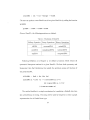
4.5
MyTable Module
The system is capable of computing all integral homogeneous relation algebras with
n atoms and s symmetric atoms. In order to do so, the system checks the properties
of Theorem 7 for all possible sets of cycles. The result is saved in a list on the hard
disc.
During the computing process, the system could be stopped at any point. If we did
not save our data before the system was halted, we would have to compute the same
data again. For optimization reasons, the system is designed to handle unexpected
halt.
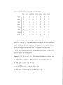
We imagine that there is a table in our system like Figure 4.5. Given nand s,
there are 2Q (n,s) possible sets of cycles where Q( n, 8)
= ~ (n
- 1) [( n - 1)2 + 38 - 1] are
described in [8]. The first column stores the indices of 2Q(n,s) atom structures. The
second column stores the Boolean values which indicates whether the atom structure
leads to a relation algebra. The third column stores the list indices of atom structures
that are isomorphic to the current one.
Table 4.5: MyTable
Index I isRA I Isomorphic List I
1
T
[2]
2
T
[1]
3
F
[18,19,20]
2Q (n,s)
F
[]
52
Recall that any two complete and atomic relation algebras are isomorphic to each
other if and only if their atom structures are isomorphic. In our example in Figure
4.5, we already have computed the first row and it is isomorphic to the second row,
so that
it is not necessary to compute the Boolean value isRA for this atom structure
,
again.
Our implementation does not use the same kind of table as in Figure 4.5, since
such a table would become extremely large for larger numbers of atoms. We only
use one byte to represent one row in the table above and we write them in sequential
order.
So far we have just computed this table for n
=
6 and s
=
2. For further comments
on the limitation of the system with respect to the value of nand s see Chapter 6.
Since there are 2Q (n,s) possible sets of cycles, it is easy to represent the index of
atom structures in Q(n, s) binary form.
For example, given n = 4 and s = 2, then the set of all possible cycles is:
[(2,2,2), (2, 2, 3), (2,3,3), (2,3,4), (2,4,4), (3,3,3), (3,3,4)]
where each ternary in the set represents its own cycle set.
The atom structure [(2,4,4), (3, 3, 3), (3,3,4)] has index 7, which is 0000111 in
binary form.
Given an index, the indexTo function finds the corresponding ternary list.
indexTo :: Int -> Int -> Integer -> Cycle
indexTo n s i
where list
len
I i«2-len)
= [tl(b,t) <- list,b ==
1]
= zip (bList len (binary i)) (allCycles (converse n s) n)
= qNS
n s
53
Given a ternary list, the fromlndex function finds the corresponding index number.
fromIndex :: Int -> Int -> Cycle -> Integer
.fromIndex n s ts
ts
[]
ts /= []
where list
len
= 0
= decimal [bl(b,t) <-(update n s ts list)]
= zip (bList len (binary 0)) (allCycles (converse n s) n)
= qNS n s
We implemented the isomorphic list in the following steps: First, find the atom
structures at the given index and convert the given index to a Q(n, s) binary form.
Secondly, find all map functions for atoms, then apply every map function on each
cycle of the atom structures componentwise; after that we will receive a list of new
atom structures. Finally, find the indices for each new atom structures and sort the
list, so that the first element is the minimum isomorphic index.
Note that we obtain all map functions by calling mapFunctions. It simply combines the direct product of the symmetric atoms' permutation list and the asymmetric
atoms' permutation list.
mapFunctions :: Int -> Int -> [[Int]]
mapFunctions n s
where sList
= sList
'combine' asList [[x,x+1] I x <- [s+1,s+3 .. n]]
= permutations [2 .. s]
asList 1 = concatMap (\x->foldl combine [[]] (map permutations x))
(permutations 1)
In the MyTable module, we define a new data type Table by given a handle and
a start position of the file.
54
newtype Table
type RATable
= Tab (Handle,Int)
= MVar Table
We will create a new Table without filling the isRA field if no such a file exists.
Otherwise we will load a Table from an existing file.
Haskell I/O Handle allows us to perform specific operations at any locations in
the file.
The function getRAValue will return isRA value in the given Table at the index
getRAValue :: RATable -> Integer -> 10 (Maybe Bool)
Given a Table, Handle Position, isRA Value, the function updateRATable updates
the Table value at the file position
updateRATable :: RATable -> Integer -> Bool -> 10 ()
Haskell maintains internal buffers for files. Our data may not be flushed out to
the operating system until we call closeRATable.
closeRATable :: RATable -> 10 ()
4.6
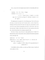
GUI
The framework of the graphic user interface is developed using Glade which is an
interface designer that allows the user to graphically layout an application window
and its dialogs. Below in Figure 4.2 there is a screenshot of Glade during the design
of the graphical user interface of our system. Glade saves the interface in XML files,
that will be loaded by the application at runtime.
The library Gtk2Hs is the Haskell binding for GTK and Glade.
55
(~
Figure 4.2: The Framework of GUI
import qualified Graphics.UI.Gtk.Glade as Glade
Just xml <- Glade .xmlNew "My_GUI.glade"
window <- Glade.xmlGetWidget xml Gtk.castToWindow "window!"
The Haskell code above shows how to import and use the user interface designed
in Glade. First, we have to import the module Graphics. UI. Gtk. Glade. The XML
file generated by Glade is loaded in the next line, and finally, the main window is
created using its name used within Glade. For further details of developing and using
graphical user interfaces with Glade and Haskell we refer to [12] .
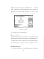
The system interface is made up of four main parts: the graph display area, the
system message box, the internal list of algebras created so far , and the user input
area.
The graph display area shows result pictures which are corresponding to the user
inputs. By selecting an item in the NA list store,the corresponding picture will be
displayed in the graph display area. Each NA structure has a to String method that
56
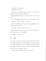
can convert the data type into the Dot language. Figure 4.3 shows the running
process. The Dot language is used by Graphviz (a graph visualization software) to
generate pictures. For further details we refer to [6].
Graphviz
Create Graphs
Figure 4.3: Running Process
The system message box shows system messages which helps the user to understand each step of the system operations. It displays error messages, file location
messages, and user Input/Output messages.
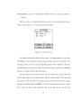
The internal list of algebras store presents the internal process results. It allow
the user to choose items in the list. Those chosen items can be used for creating a
CombineNA structure, deleting, or saving as a xml file.
57
,
Chapter 5
User Manual
In this chapter, we present how to use our system. We start by giving a brief overview
of the system. After that we describe how we organize the system documents. At the
end, we give a thorough example to demonstrate our system.
5.1
Overview
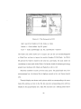
The system was intended for generating finite integral relation algebras using Windows operating system. It provides graph representations to visualize different structures of finite integral relation algebras. The system has interrupt capability to handle
unexpected halting. It allows the users to save their final results as files in xml format. The intermediate results and structure graphs are available for reloading. The
system has an easy to use graphical user interface. Figure 5.1 is a screenshot of the
system's graphical user interface.
58
.,
~
'SplitNA
~
CCimbintNAO *'.3
~
Coml:intNAl
#2
#"
~:~,;::~:e::t,~";7::'~~~,~:!i~~l':='I'l~won Argtbras.
'~,"'on
'",m",'\i, ""':l
Figure 5.1: Graphic User Interface.
5.2
User Instruction
In order to run our system properly, the user has to install a GUI library which is
called Gtk2Hs. The user should consult the gtk2hs downloads site at
http://www.haskell.org/gtk2hs/downloadj.
In order to create a homogeneous relation algebra, the user should specify the
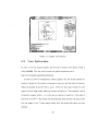
number of atoms (n), the number of symmetric atoms (s), and the index of structure
within all possible structures with nand s. There are three spin buttons for user
input in the top right corner which can be seen in Figure 5.2. Two numbers nand n
are positive integers which n - s is even and n is greater or equal to s. The index is
start from 0 to 2Q (n,s). The system will automatically check whether the input index
is in the range or not. If user inputs invalid data, the system will report an error
message:
59
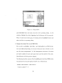
Figure 5.2: User Input Area.
"Invalid Input Data. (1<=S<=N && even (N-S) &&
O<=i<2~Q(N,S»"
The messages will be displayed by the system message box at the bottom left
corner of the GUI. Furthermore, when the user applies any kind of operations, the
system message box will also display the correspondent messages. Below the user
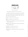
input area, there are eight operation buttons.
HomNA: create a HomNA and save in the NA list below.
SplitNA: create a SpiitNA and save in the NA list below.
CombineNAO: create a CombineNA which has 0 inter atom in the hom-sets between
objects of different inner NAs.
CombineNAl: create a CombineNA which has 1 inter atom in the hom-sets between
objects of different inner NAs.
ProductHNA: given two HomNAs, produce a new one.
ProductSNA: given two SplitNAs, produce a new one.
ProductCNAO: given two CombineNAs which both have 0 inter atom, produce a
new one.
60
ProductCNAl: given two CombineNAs which both have 1 inter atom, produce a
new one.
There is a view on the right side which shows all the NAs currently stored in the
system, like in Figure 5.3. In our case, there are two NAs.
The list ·of NAs
~~>()ice 0> TXp~.o ....,. .. !rI.dic;~ .
li¥J HomNA # 1
~
SplitNA
#2.
Figure 5.3: List Store Area.
The Choice indicates whether the NA is chosen. The Type means the type of NA.
The Indices is the current NA's index amount all NAs be stored in the system. By
selecting an item in the view, the corresponding picture will be displayed. The user
has the freedom to choose a list of NAs which would be used for creating a CombineNA
structure or would be deleted from the system.
The user also is free to choose an NA to save as an XML file , and the XML file
will be used as inputs of the other system which is called ReIAIM. When the user
saves a NA to a file, the system will ask for the file name and the name of the output
structure (the default name is hetRel). Not only is the user able to save the current
list to a file , but also to load a list from a file. At the end, the user can close the
61
program by clicking on the Quit button.
5.3
File Organization
,
There are two root directories. The first one is System, the second one is Algebras.
The System contains all the intermediate files are created by the system during the
generation of the finite relation algebras. These files are only used by the system.
Docs: contains the Haskell source code documentation of the system.
IsoMap: contains all Isomorphisms of the given RA.
RAs: contains the RA tables.
Algebras contains all the intermediate files created by the system during the
representation of the finite relation algebras. These files may be used by an external
program.
Dot File: contains dot files used by an external program . .
Graph: contains graph representations for NA Structures.
NaList: contains the lists of NA which are loaded by the system.
XML: contains the information about heterogeneous relation algebras.
5.4
Example
In this section we provide a thorough example for the use of the system. In this
example we apply all kinds of operations and save the result in different formats.
62
1. Create a HomNA:
First, we are going to create a homogeneous relation algebra. After selecting
n=4 and s=2 in the input area on the top right corner of the graphical user interface, the proper index range, i.e., 0-127, is displayed. We select 6 as the index
and press the button labeled 'HomNA'. The system creates the corresponding
structure, adds it to the list of structures in the lower left corner, and displays
the result as shown in Figure 5.4.
HomNA
~
j'l Progran, th.tgenfrating Finit~ Jntf9r.l Re.lation Algebra5.
he- Tot.1 number of Non hcnlorphic RAt: 37
tf.ateaHomNA.
Figure 5.4: HomNA 6@(4,2)
If this is the first time ever that a homogeneous relation algebra with 4 atoms
and 2 symmetric atoms is generated, the system will generate the files 'IsoMapA_2'
in the folder 'IsoMap' and the file 'RAsA_2 ' in the folder 'RAs ' as described
in Chapter 4. Notice that this may take some time depending on Nand S. In
addition, the system will produce two file related to the image shown in Figure
5.4. These files are the file 'HomNA1.dot' in the folder 'DotFile', and the file
'HomNA1.png' in the folder 'Graph'.
63
2. Create a SplitNA:
Secondly, we create an instance of the SpiitNA structure. Similar to creation
of the first structure we enter N=3 and S=1 on the top right corner. Again,
the proper index range (0-3) is displayed, and we select 3. This time we press
the button labeled 'SplitNA'. As before the system generates the structure and
displays it as a graph as seen in Figure 5.5. The system will generate similar files
SplitNA
i~ iI
Program that grnerating Finitl! Integr~1 Relatiol1 Ai gebra~.
=
he Total numb6 of Non I~omorphic RAs 3
tutl: • .sp~tNA
Figure 5.5: SplitNA 3@(3,1)
as in our first example on the disc. This time the files are called 'IsoMap_3_1',
'RAs3_1', 'SplitNA2.dot' and 'SplitNA2.png', of course.
3. Create a CombineN A:
So far, we have created two algebras which are stored in the internal list of
algebras. Now we use those algebras in order to build a more complex structure. First, we select the previous two structures in the list of algebras in the
lower right corner of the application. Then we press the button labeled 'Com-
64
BineNAO', and the system will create a CombinNAO structure. A new algebra
called 'ComBineNAO #3' is created and added to the list . We select this new
algebra and press the button labeled 'CombineNA1'. The result is shown in
Figure 5.6. This time the system only generates the dot and png files for the
i, I Program lhat'genua6ng Fi~ite in1egrill Refation.Alg~bfiS.
Totil nunlbf:r Qf rfon.lso.n lorphic RAs., 37
bf N'on ls"pmorphic ItA!; =,3
Figure 5.6: CombineNA
two new algebras in the corresponding folders.
4. Product of two NAs:
In order to demonstrate the product functions, the user should have already
created at least two structures of the same type. For example in Figure 5.7
the algebras HomNA 1@(2,2) and HomNA 3@(3,1) have already been created,
and the algebra HomNA 20503@(6,2) was obtained by using the ProductHNA
function. As before, dot and png files were created during this process.
5. Save and Load NA List:
The system has created seven NAs in the list since its inception. To save them,
65
HomNA
,is,. P~fam ~t generating finitelntt.~ril~RdlJtion A1g~t.s.
he lotJlnunibu ~f Nonl!omorp,hic RAs= 2
t9te.aHorylNA
he 1.tlti!'1 "'Imber cf Non Jsomo~t: RAs ::: 3
reatellHomNA
.
1>:~:~;:~~;:;~;::GmNAi'Pfl9
I~
"nlNAl.p.ng
reate a new HomNA which i5.'produc.t-of twit ~e_[ ed~ !.Iomt:-jAs
Figure 5.7: ProductHNA
press SaveList button and name your file in the upcoming dialog. In the
subfolder NaList of the folder Algebras the file NAseven will be generated.
When we need to use the list again, we should press the LoadList button and
select the file in the upcoming dialog.
6. Output the chosen NA as an XML File:
We are able to save HomNAs, Spli tNAs, and CombineNAs in an XML format.
The only difference depending on the kind of structure that is stored is in the
way the atoms are represented. In the heterogeneous structures, the atoms
are triples consisting of source and target object and the number of the atom.
(Recall Section 4.3 of the previous chapter).
The following shows the content of the file hetH.xml in the folder XML which
was generated by saving the algebra HomNA #1 in XML format.
<hetRel name="hetRel#1" isRA="False">
<objects number="1" />
66
<atoms source="O" target="O" number="4" symmetric="2" />
<cycles>
«0,0,1),(0,0,1),(0,0,1»
«0,0,1),(0,0,2),(0,0,2»
«0,0,1),(0,0,3),(0,0,3»
«0,0,1),(0,0,4),(0,0,4»
«0,0,2),(0,0,4),(0,0,4»
«0,0,3),(0,0,3),(0,0,3»
</cycles>
</hetRel>
The next example shows the content of the file 'hetS.xml' which was generated
by saving the algebra SplitNA #2 in XML format.
<hetRel name="hetRel#2" isRA="True">
<objects number="3" />
<atoms source="O" target="O" number="O" symmetric="O" />
<atoms source="O" target=" 1" number="O" />
<atoms source="O" target="2" number="O" />
<atoms source="1" target="O" number="O" />
<atoms source="1" target="l" number="3" symmetric="1" />
<atoms source="1" target="2" number="l" />
<atoms source="2" target="O" number="O" />
<atoms source="2" target="l" number="l" />
<atoms source="2" target="2" number="l" symmetric="l" />
<cycles>
«1,1,1),(1,1,1),(1,1,1»
«1,1,1),(1,1,2),(1,1,2»
«1,1,1),(1,1,3),(1,1,3»
«1,1,1),(1,2,1),(1,2,1»
«1,1,2),(1,1,1),(1,1,2»
«1,1,2),(1,1,2),(1,1,2»
67
«1,1,2),(1,1,2),(1,1,3)) «1,1,2),(1,1,3),(1,1,1))
«1,1,2),(1,1,3),(1,1,2)) «1,1,2),(1,1,3),(1,1,3))
«1,1,2),(1,2,1),(1,2,1)) «1,1,3),(1,1,1),(1,1,3))
«1,1,3),(1,1,2),(1,1,1)) «1,1,3),(1,1,2),(1,1,2))
«1,1,3),(1,1,2),(1,1,3)) «1,1,3),(1,1,3),(1,1,2))
«1,1,3),(1,1,3),(1,1,3)) «1,1,3),(1,2,1),(1,2,1))
«1,2,1),(2,1,1),(1,1,1)) «1,2,1),(2,1,1),(1,1,2))
«1,2,1),(2,1,1),(1,1,3)) «1,2,1),(2,2,1),(1,2,1))
«2,1,1),(1,1,1),(2,1,1)) «2,1,1),(1,1,2),(2,1,1))
«2,1,1),(1,1,3),(2,1,1)) «2,1,1),(1,2,1),(2,2,1))
«2,2,1),(2,1,1),(2,1,1)) «2,2,1),(2,2,1),(2,2,1))
</cycles>
</hetRel>
Our final example shows the content of the file 'hetC.xml' which was generated
by saving the algebra CombineNAO #3 in XML format.
<hetRel name="hetRel#3" isRA="False">
<objects number="4" />
<atoms source="O" target="O" number="4" symmetric="2" />
<atoms source="1" target="1" number="O" symmetric="O" />
<atoms source="1" target="2" number="O" />
<atoms source=" 1" target="3" number="O" />
<atoms source="2" target="1" number="O" />
<atoms source="2" target="2" number="3" symmetric="1" />
<atoms source="2" target="3" number="1" />
68
<atoms source="3" target="l" number="O" />
<atoms source="3" target="2" number="l" />
<atoms source="3" target="3" number="l" symmetric="l" />
<cycles>
«0,0,1),(0,0,1),(0,0,1)) «0,0,1),(0,0,2),(0,0,2))
«0,0,1),(0,0,3),(0,0,3)) «0,0,1),(0,0,4),(0,0,4))
«0,0,2),(0,0,4),(0,0,4)) «0,0,3),(0,0,3),(0,0,3))
«2,2,1),(2,2,1),(2,2,1)) «2,2,1),(2,2,2),(2,2,2))
«2,2,1),(2,2,3),(2,2,3)) «2,2,1),(2,3,1),(2,3,1))
«2,2,2),(2,2,1),(2,2,2)) «2,2,2),(2,2,2),(2,2,2))
«2,2,2),(2,2,2),(2,2,3)) «2,2,2),(2,2,3),(2,2,1))
«2,2,2),(2,2,3),(2,2,2)) «2,2,2),(2,2,3),(2,2,3))
«2,2,2),(2,3,1),(2,3,1)) «2,2,3),(2,2,1),(2,2,3))
«2,2,3),(2,2,2),(2,2,1)) «2,2,3),(2,2,2),(2,2,2))
«2,2,3),(2,2,2),(2,2,3)) «2,2,3),(2,2,3),(2,2,2))
«2,2,3),(2,2,3),(2,2,3)) «2,2,3),(2,3,1),(2,3,1))
«2,3,1),(3,2,1),(2,2,1)) «2,3,1),(3,2,1),(2,2,2))
«2,3,1),(3,2,1),(2,2,3)) «2,3,1),(3,3,1),(2,3,1))
«3,2,1),(2,2,1),(3,2,1)) «3,2,1),(2,2,2),(3,2,1))
«3,2,1),(2,2,3),(3,2,1)) «3,2,1),(2,3,1),(3,3,1))
«3,3,1),(3,2,1),(3,2,1)) «3,3,1),(3,3,1),(3,3,1))
</cycles>
</hetRel>
69
Chapter 6
Conclusions
This chapter begins with a summary of the work in this thesis and the conclusions
reached. This is followed by a discussion of the areas that require further investigation
and the work planned in the future.
6.1
Summary
In this thesis, we focused on generating atom structures of finite integral heterogeneous relation algebras. We were able to define three new data types and operations
representing such structures. Following the theoretical work, we have implemented
a Haskell library which can be used to compute atom structures of finite integral
relation algebras. In addition, we have developed a system with a graphical user interface that allows users to create, visualize, and store such atom structures for later
use. Except for a simple program enumerating the non-isomorphic integral homogenous relation algebras up to six atoms [9], the system developed in this thesis is the
first of its kind. In particular, there is no system that generates any heterogeneous
70
structures. However, the results of our system, i.e., the algebras constructed, can
be used by the system developed by Z. Ahmed in [1]. His program allows users to
execute computations in matrix algebras where the coefficients are relations from a
heterogeneous integral relation algebra. Recall that every algebra is equivalent to a
matrix algebra.
6.2
Future Work
The current system also has its limitations. The huge amount of homogenous integral
relation algebras for n > 5 makes it almost impossible to use any algebras of that
size. In fact, the number of non-isomorphic relation algebras with n
= 6 and s = 6 is
already 3,849,820. For any n > 6 the number of algebras is still unknown [9].
Although we have accomplished a lot in this thesis, there is room for additional
work, which can be built on the current implementation. Some of these ideas are
presented below.
Concurrency: The computation of all atom structures with n atoms could be done
using multiple threads or even multiple computers in order to gain a significant
speed up. The current state of concurrency in Haskell did not allow us to
implement this feature so far.
External implementation: This point is related to the first one. Instead of using
the concurrency of Haskell, one could implement the search of all atom structures with n atoms in a different language. Since efficiency is crucial in that task
a suitable language could be C or
C++. The functionality of those programs
71
could be utilized within Haskell by using the foreign function interface FFI. In
addition, this C or C++ program could be a parallel program.
More kinds of unions: We have implemented two kinds of unions of heterogenous
, relation algebras, the direct and the enlarged sum. These two structures introduce 0 and 1 atom in between the input algebras, respectively. There are
examples of a basis that has larger intermediate structures. For example, the
number ofrelations between two objects A and B in a SplitNA is usually larger
than 2. These objects are HomNAs themselves so that it should be possible to
create the algebra consisting of A and B and all relations between using a sum.
How to create such algebras in general is unknown so far, and subject of further
research.
72
,
Bibliography
[1] Z. Ahmed. Realm - a system to manipulate relations. Master's thesis, Brock
University, 2009.
[2] R. Bird and O. de Moor. Algebra of Programming. Prentice-Hall, 1997.
[3] G. Brikhoff. Lattice Theory. AMS, third edition, 1995.
[4] 1. Diintsch. Relation algebras and their application in temporal and spatial
reasoning. Artificial Inteligence Review, 23:315-357, 2005.
[5] P. Freyd and A. Scedrov. Categories, Allegories. North-Holland, 1990.
[6] E. Gansner, E. Koutsofios, and S. North. Drawing graphs with dot, January 2006.
[7] S. Koppelberg. General Theory of Boolean Algebras. North Holland, 1989.
[8] R. D. Maddux. Finite integral relation algebras. In Lecture Notes in Mathematics
1149, pages 175-197. Springer-Verlag, 1985.
[9J R. D. Maddux. Relation Algebras, volume 150 of Studies in Logic and the Foundations of Mathematics. Elsevier Science, 2006.
73
[10] G. Schmidt, C. Hattensperger, and M. Winter. Heterogeneous relation alge-
bras. In C.Brink, W.Kahl, and G.Schmidt, editors, Relational Methods in Computer Science, Advances In Computing Science, chapter 2, pages 39-53. Springer-
Verlag, 1997.
[11] G. Schmidt and T. Strohlein. Relations and Graphs. Discrete Mathematics for
Computer Scientists. EATCS Monographs in Theoretical Computer Science.
Springer-Verlag, 1993.
[12] B. O. Sullivan, J. Goerzen, and D. Stewart. Real World Haskell. Oreilly, first
edition, November 2008.
[13] A. Tarski and S. Givant.
A Formalization of Set Theory without Variables.
Handbook of Boolean Algebras (Vol. 1). AMS, 1988.
[14] M. Winter. Relation algebras are matrix algebras over a suitable basis. Technical
Report 1998-05, UniversiUit der Bundeswehr Miinchen, November 1998.
[15] M. Winter. A pseudo representation theorem for various categories of relations.
TAC Theory and Applications of Categories, 7(2):23-37, 2000.
[16] M. Winter. Products in categories of relations. The Journal of Logic and Algebraic Programming, pages 145- 159, 2008.
[17] S. Zhang and M. Winter. Three structures for generating finite integral relation
algebras. PhD Program of RelMiCSjAKA, pages 28-32, 2009.
74