Download Computational Solid State Chemistry

Computational Solid State Chemistry 1 1 Computer Experiment 16: Computational Solid State Chemistry 1.1 Background This experiment gives an introduction to the quantum chemical simulation of solids and surfaces. The goal of the experiment is to show the characteristics of the methods and models used in solid state chemistry which differ from those in molecular quantum chemistry. 1.1.1
Periodic models The aim of theoretical solid state chemistry is to predict the properties of condensed matter. In reality solids are always of finite size. However, at the atomic scale the macroscopic dimensions of real crystals and crystallites (usually with diameters in the range µm to cm) are so large that they can be assumed as infinite. At the same time the number of atoms even of the smallest crystallites (at least 109) is prohibitively large to be fully treated by molecular quantum chemical techniques. The problem can be solved if high long-­‐range order is assumed as it is the case in many crystalline solids. In that case the atoms form a periodic lattice. Its basic building block is a finite arrangement of atoms, the so-­‐called repeat unit. For a perfect solid without defects or impurities the smallest possible repeat unit, the primitive unit cell, can be used. It contains by definition the smallest possible number of atoms that fully build up the lattice by an infinite number of translations in three dimensions in terms of three primitive lattice vectors (a, b and c). The vectors connect translationally equivalent atoms. Depending on the relative size of the three vectors and the angles (α, β, γ) between them, the corresponding lattices are classified into seven crystal systems (cubic, hexagonal, rhombohedral, tetragonal, orthorhombic, monoclinic, triclinic). 1.1.2
Bloch functions The consequence for quantum chemistry is that the nuclear potential V of the Hamilton operator contains an infinite number of nuclei in a periodic arrangement. In terms of a general lattice vector T= naa + nbb + ncc which connects two primitive unit cells it follows that V(R +T ) =V(R) (R is a position vector in the three-­‐dimensional space). Therefore the wavefunction is necessarily also periodic. It must obey the following periodic boundary condition formulated by Bloch as Bloch theorem. It states that the Computational Solid State Chemistry 2 wavefunction Ψ in two unit cells is identical except a phase factor (the “complex 1”) e ik•T : !(R +T ) = e ik•T !(R) . Here k is the so-­‐called wave vector (note the scalar product). The wavefunction can be expressed as a product of a periodic function Φ, called Bloch function and a phase factor in Cartesian space: ! = e ik•R "(R) with !(R +T ) = !(R) . In principle, the components of the wave vector k can assume any value resulting in an infinite number of Bloch functions. In practical periodic calculations, however, one restricts the k vectors to a finite number in a limited space, the irreducible Brillouin zone. The basic idea is that a large but finite region (the main region with translation vectors P = N aa + N bb + N cc ; the Ni are large integer numbers) is considered as a representative for the periodic lattice. The wavefunction of this region is periodic in Cartesian space !(R + P) = !(R) (Born-­‐von Kármán condition). The condition e ik•P = 1 implies that the special k vectors κ fulfil the following relation: !=
sa
Na
a '+
sb
Nb
b '+
sc
Nc
c ' where the si are integer numbers ranging from 0 to Ni-­‐1, and a’, b’ and c’ are vectors of the reciprocal space. They are defined as a ' =
2!
(b !c) etc. V
where V is the primitive cell volume. There are special schemes (e.g. by Monkhorst and Pack) for the selection of special κ vectors. For the calculation of wavefunction-­‐based properties the integration over an infinite number of k vectors is replaced by a summation over the special κ vectors: 1
V
#
dk !
1
N
N
"!
j
j
. In practice this means that the choice of the Ni will affect the results of the calculation. Since for each κ vector a wavefunction has to be calculated in a self-­‐consistent-­‐field procedure similar to molecular quantum chemical methods, the total number N= Na Nb Nc will linearly increase the computational effort. On the other hand, a larger number of κ vectors will lead to more accurate results. In every case convergence tests have to be performed. 1.1.3
Cyclic cluster model There are two equivalent ways to reach convergence with the number of κ vectors (also called κ points): in usual periodic calculations for perfect crystals as described above one starts from the primitive unit cell and increases the main region via the Na, Nb, Nc. An alternative is to increase the size of the repeat unit. A supercell consists of several primitive unit cells. The translation vectors of the supercell are multiples of the Computational Solid State Chemistry 3 primitive lattice vectors. Accordingly, the factors Na, Nb, Nc become smaller and therefore the number of κ vectors of a supercell can be smaller than in a primitive cell to reach the same accuracy. Of course, this is at the cost of larger matrices for the calculation of the wavefunction in the supercell compared to the primitive cell, similar as for molecular systems. In the extreme case the supercell contains Na×Nb×Nc primitive unit cells and is identical to the main region. In this limit it is sufficient to use only a single κ vector ! = 0 , the so-­‐called Gamma (Γ) point. This is exactly the basic idea of the cyclic cluster model. A large supercell is taken as model for the crystalline solid and a Gamma-­‐only periodic calculation is performed. All quantities (orbital coefficients, matrix elements) are real numbers. The main difference between cyclic cluster and conventional periodic Gamma-­‐only calculations is the definition of the interaction regions. In conventional periodic calculations many-­‐center integrals (e.g. nuclear attraction or Coulomb integrals) that involve a particular atom are calculated within a spherical region. Its radius is defined by a preselected cut-­‐off value for certain types of integrals (in most cases overlap integrals). Again the choice of this threshold is crucial for the quality of the results and its convergence behaviour must be carefully checked in each case. At variance, in the cyclic cluster model the interaction region around each atom is precisely defined by the translation vectors of the supercell. They are used to define a Wigner-­‐Seitz cell around each atom. Each point within a Wigner-­‐Seitz cell is by construction closer to the central lattice point than to any translationally equivalent lattice point outside. For this reason convergence of calculated properties with respect to the size of the cyclic cluster must be checked for each system under investigation. (Further reading: C. Kittel, Quantum Theory of Solids, John Wiley & Sons, 1987) 1.1.4
MSINDO CCM calculations The Cyclic Cluster Model (CCM) has so far been implemented only in semiempirical methods due to the large computational effort of the large supercell wavefunction calculation. A recent example is the MSINDO implementation (for literature see section 1.3). 1.2 Description of the Experiment In principle the input specification of a cyclic cluster is the same as for a molecule. A few additional keywords are required in section 1: Computational Solid State Chemistry 4 # Section 1: keywords for CCM
CCM CUBIC3D # For three-dimensional periodic cyclic
# cluster calculations of cubic lattices
VECTA(NA1,NA2) VECTB(NB1,NB2) VECTC(NC1,NC2)
# The three supercell translation vectors a,b,c
# They are defined by two atoms Nx1 and Nx2
# according to their numbers in the input.
The at most 6 atoms (with numbers NA1, NA2, NB1, NB2, NC1, NC2; note that it is possible but not necessary to set NA1=NB1=NC1) used for the definition of the translation vectors must be dummy atoms (with atomic symbol X or atomic number 0). This is particularly important for geometry optimizations where normal atoms change their positions which will also change the translation vectors in an unwanted way. The positions of dummy atoms are not changed during optimizations. The cyclic cluster must not contain translationally equivalent atoms. Therefore the three vectors must point “outside” the cluster. It is convenient to place one dummy atom (the starting point of a vector) “above” one of the normal cluster atoms and to place the second at the position of the nearest translationally equivalent lattice point outside the cluster. If the cluster atoms are defined by a Z-­‐Matrix input, the additional dummy atoms must be defined with the same set of internal coordinates as the corresponding “real” cluster atoms. In the following the smallest possible CCM for cubic magnesium oxide (MgO) is shown. MgO 2x2x2 minimal 3D CCM :NEW
RHF
CCM CUBIC3D VECTA(9,10) VECTB(9,11) VECTC(9,12)
OPT (ANALY cannot be used for CCM internal optimization)
:END
1 Mg
1 2 O RMgO
1 2 3 Mg RMgO 90
1 2 3 4 O RMgO 90
0
3 2 1 5 O RMgO 90 90
4 3 2 6 Mg RMgO 90 90
1 4 3 7 O RMgO 90 90
2 1 4 8 Mg RMgO 90 90
4 3 2 9 X RMgO 90
0
# X9 is above Mg1
3 1 2 10 X RMgO 180 180
# end point of vector a
3 1 4 11 X RMgO 180 180
# end point of vector b
3 1 5 12 X RMgO 180 180
# end point of vector c
:END
RMgO = 2.15 # the conventional lattice vector is 2*RMgO
:END
END
From such a calculation the MgO lattice constant a=2 RMgO (experimental value: a=4.212 Ǻ [CRC]) and the energy of atomization !a E can be determined. !a E is the Computational Solid State Chemistry 5 CCM Binding Energy (with respect to the free gas phase atoms) as given in the output (after optimization!) devided by the number of formula units (in the present example 4). In the literature it is given in kJ/mol. MSINDO prints energies in atomic units (Hartrees). The experimental heat of atomization to which the calculated results is to be compared can be obtained from experimental heats of formation of MgO and the free Mg and O atoms (e.g. from the NIST web page http://webbook.nist.gov/chemistry/form-­‐ser.html). !a H exp (MgO,c) = "! f H exp (MgO,c) + ! f H exp (Mg,g) + ! f H exp (O,g) = 601.6+147.1+249.2 = 997.9 kJ/mol As spectroscopic property MSINDO CCM provides an approximation of the smallest optical transition energy, he so-­‐called band gap. It is approximated as energy difference between the highest occupied crystalline orbital (HOCO) and the smallest of all corrected virtual orbital energies (expectation values of IVO-­‐operator for excitation from HOCO). The Huzinaga correction corresponds to a minimal configuration interaction of the HOCO and the corresponding virtual orbital. The experimental band gap of crystalline MgO is 7.8 eV. It cannot be expected that the small cyclic cluster given above provides accurate results, not even within the limits of the approximate semiempirical scheme. Therefore the computer experiment consists of a convergence test of the mentioned observables with cyclic cluster size. For this purpose the program mgoinp is available for the construction of MgO clusters. However, this program only generates molecular clusters. The CCM keywords and translation vectors have to be added accordingly. The same cluster model can be used to obtain structural and energetic information from the most prominent MgO(001) surface. Here the three ciphers correspond to Miller indices. (001) indicates that the surface is parallel to the ab plane. In the cubic rocksalt structure which is common for, e.g., MgO, CaO, NaCl, KBr, (100), (010) and (001) planes are equivalent. The necessary changes in the MSINDO CCM input are rather small: Computational Solid State Chemistry 6 MgO 2x2x2 minimal (001) 2D CCM :NEW
RHF
CCM CUBIC2D VECTA(9,10) VECTB(9,11) VECTC(9,12)
CARTOPT ANALY LSTE=100 # No. of Cartesian opt. steps
:END
1 Mg
1 2 O RMgO
1 2 3 Mg RMgO 90
1 2 3 4 O RMgO 90
0
3 2 1 5 O RMgO 90 90
4 3 2 6 Mg RMgO 90 90
1 4 3 7 O RMgO 90 90
2 1 4 8 Mg RMgO 90 90
4 3 2 9 X RMgO 90
0
3 1 2 10 X RMgO 180 180
3 1 4 11 X RMgO 180 180
3 1 5 12 X RMgO 180 180
:END
RMgO = 1.9672 # must be the 3D optimized value of the same
# cluster
:END
END
In CCM surface calculations one must be aware that the model is finite in the dimension normal to the surface plane (a so-­‐called slab model). In general the number of layers has an important effect on all calculated surface properties, and convergence must be checked. Of general interest are three properties, the surface energy Es , the relaxation δd, and rumpling Δ. The surface energy is the difference between the CCM Binding energies of the (optimized!) two-­‐dimensional and three-­‐dimensional cyclic clusters, normalized to the surface area A of the 2D cluster (given in the output file). Es = (E B2D ! E B3D ) / 2A The factor of 2 comes from the fact that the model has two surfaces. Since the stabilization of surface atoms by chemical bonds and electrostatic interactions (Madelung field) is in general smaller as in the 3D bulk, the surface energy is positive. Conversion factor from Hartree/Ǻ2 to SI unit J/m2: 436.0
Surface relaxation is defined as the relative change of the vertical distance between the first and second layer d12 compared to the corresponding interlayer distance d in the bulk (here: d=RMgO as optimized in the 3D CCM calculation). The final Cartesian coordinates of all cluster atoms can be found in the file fort.9 after the 2D CCM calculation has successfully finished. The order of the atoms corresponds to that of the input. Dummy atoms are not printed there, but the additional atoms that were necessary to define the Wigner-­‐Seitz cells around the cluster atoms. These are indicated by atomic numbers that are increased by 100. In the 2D surface optimization it is important to use precisely the optimized RMgO value as obtained from the same cyclic cluster in the 3D Computational Solid State Chemistry 7 bulk optimization. The physical background is that the crystal lattice parameter is determined by the vast majority of “inner” bulk atoms and does not change significantly when a real crystal is cut. Any surface property calculated with another internal bond length is meaningless. In a successful surface calculation the z coordinates (normal to the surface plane) of first-­‐layer atoms of the same kind are identical. Thus there are only two zi values for each layer i, namely zi(Mg) and zi(O) in the present case. If this is not the case, it is very likely that the input contains an error. With these data, relaxation δd 12 and rumpling Δ are defined as follows: d12 = [z1(Mg) + z1(O)! z 2(Mg)! z 2(O)] / 2 !d12 = (d12 !d) / d "100 ! = [z1(O)" z1(Mg)] / d #100 In the literature both values are given in percent of the bulk interlayer distance. Experimental values for δd 12 range from -­‐0.6 to -­‐1.0 %, Δ is reported as +0.5 to +1.1 % indicating that the surface oxygen is above the surface magnesium, Es is between 55 and 63 J/m2. If the calculated bulk and surface properties are in reasonable agreement with experiment, confidence is gained that the underlying model and method of calculation is sufficiently accurate to model the more difficult task of adsorption of molecules at the surface. A particular example is the adsorption of a rather simple molecule, CO, on the MgO(001) surface. Over two decades the measured and calculated adsorption energy, and even the adsorption structure, as published in the literature, changed dramatically from year to year. Now there is general agreement that at low coverages CO sits vertically above a surface magnesium and is bonded via the carbon atom with an adsorption energy of about 15 kJ/mol. At higher coverages overlayer structures due to tilting of the CO molecules are observed. With MSINDO CCM the adsorption of molecules at surfaces requires only moderate changes in the input. Starting from the 2D calculation as described above, the CO molecule can be added to atoms in the first layer by expanding the Z-­‐Matrix correspondingly. Some help can be obtained from the Molden Z-­‐
Matrix editor; unfortunately it does not give the MSINDO Z-­‐Matrix convention as output. But it can be used to check the correct orientation of a selected set of internal coordinates. Since it is known that CO sits vertically above the surface, a convenient Computational Solid State Chemistry 8 definition is via pairs of subsurface and surface atoms with 180 degrees angles. Besides the adsorption structure the most interesting property is the adsorption energy Eads, defined as difference of the 2D-­‐CCM Binding Energies of the combined system (MgO)n+CO and the free MgO surface, plus the binding energy of the free gas phase CO molecule (after optimization of RCO). For the simulation of adsorption at surfaces, a slightly different optimization strategy must be applied in the 2D CCM calculations. Since the molecule is adsorbed only on one side of the slab model, the opposite side can be used in a different sense as before. It is common use in adsorption calculations to fix the positions of those atomic layers of the slab model that are “opposite” to the adsorbed molecule so that they simulate the bulk rather than a second surface exposed to vacuum. In MSINDO it is possible to perform such restricted surface optimizations in the following way: MgO 2x2x2 minimal (001) 2D CCM first-layer relax. :NEW
RHF
CCM CUBIC2D VECTA(9,10) VECTB(9,11) VECTC(9,12)
CARTOPT CARTSLCT ANALY LSTE=100 # Opt. of selected atoms
:END
… as above
:END
RMgO = 1.9672 # must be the 3D optimized value of the same
# cluster
:END
# Total number of optimized atoms
1 2 3 4
# 4 atoms of the first layer
END
Since the number of degrees of freedom is reduced, the final CCM energy of the restricted optimization will always be higher (less negative) than that of a corresponding full Cartesian optimization of the same cluster. The same strategy (first-­‐
layer optimization only) is applied to the MgO:CO system where the C and O atoms are to be included in the optimization. Under these conditions the adsorption energy is defined as: Eads = E B2D[(MgO)n :CO]! E B2D[(MgO)n]! E gas
[CO] B
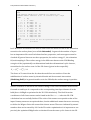
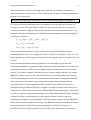
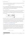
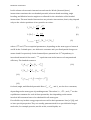
The computational experiment consists of three parts. 1. Select one of the following systems with rocksalt structure (MgO, CaO, NaCl, KCl) and calculate the bulk lattice constant, the atomization energy per unit, and the optical band gap. Be aware that reasonable starting values for RMX are required. Optimizations may fail if ones starts too far off. Use the program mgoinp in any case and modify the atomic numbers according to the system of your choice. Investigate the size convergence of the calculated bulk properties using the Computational Solid State Chemistry 9 sequence 4×4×4, 6×6×6, 8×8×8, and, if possible, 10×10×10. At which cluster size are the three bulk properties converged? Reasonable convergence thresholds are 1 kJ/mol for EB, 0.001 Ǻ for RMX, and 0.01 eV for the band gap. 2. Investigate the model dependence of the calculated surface energy, relaxation and rumpling for the sequences n×n×4, n×n×6, n×n×8 with n=4, 6, 8. Which is the smallest reasonable model? Here the criteria are 0.01 J/m2 and 0.1%. 3. Take the smallest possible model as obtained in part 2 and investigate the adsorption of CO on the (001) surface in the small coverage regime (one molecule per surface). Four possible starting structures (perpendicular above O or metal, C-­‐down or O-­‐down) are suggested, but many other are possible. What is the preferred adsorption structure for your system? 1.3 Literature 1. Roald Hoffmann, Solids and Surfaces, Wiley-­‐VCH 1989. 2. Thomas Bredow, Robert A. Evarestov, Karl Jug, Implementation of the Cyclic Cluster Model in Hartree-­‐Fock LCAO Calculations of Crystalline Systems, Phys. Stat. Sol. B 222, 495-­‐516 (2000) 3. Thomas Bredow, Gerald Geudtner, Karl Jug, Development of the cyclic cluster method for ionic systems, J. Comput. Chem. 22, 89-­‐101 (2001) 4. Florian Janetzko, Thomas Bredow, Karl Jug, Effects of Long Range Interactions in Cyclic Cluster Calculations of Metal Oxides, J. Chem. Phys. 116, 8994-­‐9004 (2002) 5. Karl Jug, Thomas Bredow, Feature Article: Models for the treatment of crystalline solids and surfaces, J. Comput. Chem. 25, 1551-­‐1567 (2004). Molecular Simulations 10 2 Computer Experiment 17: Molecular Simulations 2.1 Background Most areas of high level quantum chemistry today deal with molecules in the gas-­‐phase at zero Kelvin temperature, that is, these methods assume a rigid nuclear framework and solve the electronic structure problem in this frame. However, this point of view ignores an important fact: Real systems are subject to finite temperature, and thus, the atoms themselves exhibit dynamics! Figure 1: the water box used in the simulations. The phase behaviour of liquids, the folding of proteins, the progression of a reaction are properties that depend on the dynamics of system. With the computer capacities available today it is possible to simulate these properties in microscopic detail by following the atomic motion through time. The bridge between the dynamics of single atoms and macroscopic properties is established by applying the rules of statistical thermodynamics to the dynamic system. This experiment starts with a short introduction into how the atomic motion is treated (Newtonian dynamics), how a system is coupled to finite temperature and pressure and how the interactions between molecules are treated. In priunciple, it is possible to perform such dynamics calculations using all of the approximate methods that we have treated so far in this course. Dynamics combined with DFT methods leads to the field of “first-­‐principles dynamics”. Such calculations require extensive computer resources. We will therefore in this experiment replace the approximate solution of the electronic structure problem at fixed geometry with a much simpler approach: molecular mechanics. That is, we do not calculate the interatomic forces explicitly but instead use Molecular Simulations 11 parameterized functions that are suppose to approximate these forces and provide reasonable potential energy surfaces. The computational part of the experiment will be performed with the GROMACS package [1]. The first example will be the heating and freezing of water and an analysis of its structurural properties. In the next part a biological macromolecule is created. It is studied what happens if the system is treated either in vacuum or in solution at different temperatures. In this way protein folding will be directly visible in atomic detail. In the third part of the experiment a real protein from the protein database is simulated and analyzed. Figure 2: The helix used in the simulations. 2.1.1
Classical Dynamics The movement of particles can be described by the classical Newtonian equations of motion. A system of M atoms can be written in Cartesian space with position vectors R A = {X A,YA,Z A } for atom A. The potential energy U is a function of the position of all atoms, collectively described by R
(N )
and can so be written as ( ( )) U =U R
N
(1) The force acting on atom A , FA , is the negative partial derivative of the potential energy with respect to the nuclear coordiantes FA = !
"U
"R A
(2) Molecular Simulations 12 Since we now know the force that acts on each atom, we can use the Newtonian laws of motion in order to find the atoms trajectories:1 !! = F M AR
A
A
(3) !! the second derivative of the nuclear with M A being the mass of atom A and R
A
coordinates with respect to time. Solving this differential equation system makes it possible to propagate a system of particles through time. 2.1.2
Time Integration Having calculated the force on a particle at time t one can solve for the configuration at a future time point t + !t . There are several schemes which can be used for this purpose. The one used in the GROMACS package is the so-­‐called ‘leap-­‐frog’ algorithm. It runs as follows: "
"
!t %'
!t %' F (t )
'' = VA $$t (
'' +
VA $$$t +
!t $#
2 '&
2 '&
m
#
(4) "
!t %'
'' !t R A (t + !t ) = R A (t )+ VA $$t +
$#
2 '&
(5) Note that the velocities VA are evaluated at different points than the positions R A . This method is called leap-­‐frog algorithm because positions and velocities seem to jump over each other along the time axis. The algorithm is time reversible and fulfills certain conservation laws; Moreover, it is easy to implement and equivalent to the popular ‘Verlet’ algorithm (for a more detailed discussion see [3]). 2.1.3
Forcefield and Potential Energy Calculation The former description only states that the potential energy is a function of all atomic coordinates but does not specify how to calculate this energy. In classical molecular dynamics the energy is calculated with the aid of a ‘forcefield’. In this approach the energy depends on the atomic positions via an empirical expression of the energy. In case of the GROMACS forcefield these are seperated into bonded and non-­‐bonded interactions: U = Vbonded +Vnon!bonded 1
A trajectory is defined by the particles position
of time.
(6) ! ( t ) ) as a function
R A ( t ) and momenta (velocities VA ! R
A
Molecular Simulations 13 In this scheme electrostatic interactions and van-­‐der-­‐Waals (Lennard-­‐Jones) interactions constitute the non-­‐bonded potential, whereas bond stretching, angle bending, and dihedral torsion angles are collected for the calculation of the bonded interactions. The non-­‐bonded interactions are pairwise interactions, that is, they depend only on the relative positions of two particles at a time: (12)
VLJ (RAB ) =
VC (RAB ) =
1 q Aq B
4!"0 "r RAB
!
C AB
(7) (8) "V (R )+V (R ) (9) 12
RAB
Vnon!bonded =
(12)
(6)
C AB
LJ
A<B
6
RAB
AB
C
AB
(6)
where C AB and C AB are empirical parameters, depending on the atom-­‐types of atoms A and B. In the Coulomb part ! are dielectric constants and q are fixed partial charges on !12
atoms A and B respectively. In the Lennard Jones potential an RAB
dependency is introduced instead of the usual e
!R
AB
repulsion term in the interest of computational efficiency. The bonded terms are (
)
2
1 b
(0)
Vb (RAB ) = kAB
RAB !bAB 2
Va (!ABC ) =
(
1 !
(0)
kABC !ABC ! !ABC
2
)) ) 2
(10) (11) (
(
Vd (!ABCD ) = k! 1+ cos n! !!
(0)
(12) b
!
for bond, angle, and dihedral potential. Here kAB
, kABC
, and k! are the force constants, (0)
(0)
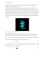
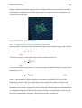
depending on the atom types of partaking atoms. The values bAB , !ABC , and ! are the equilibrium constants for each of these potentials, also depending on the atoms involved. All constants have to be tabulated for all atom types. Forcefields vary in their energy expression as well as their parameter lists (cf. [4]), and so have special properties. They are usually parameterized for a special kind of target molecules, for example proteins, nucleic acids, certain liquids, etc. Molecular Simulations 14 Using a molecular dynamics program the forcefield parameters represent the static part of the data the simulation needs. The dynamic part is comprised of the coordinates and velocities of the particles. Figure 3: A solvated protein used in the simulations. 2.1.4
Temperature and Pressure in Molecular Simulations Moving particles not only possess potential energy but also kinetic energy, both of which sum up to the total energy of the system E = K +U (13) The kinetic energy is connected to the velocities of the particles via K=
1 M
M AVA2 !
2 A=1
(14) From statistical thermodynamics it is well known that the kinetic energy is related to the temperature T via K=
1
N kT 2 eff
(15) with N eff the number of effective degrees of freedom (in principle 3N-­‐6), and k the Boltzmann constant. Thus the temperature of the systems has a direct relation to the velocity of the particles. To start with a system at a definite temperature a Maxwellian distribution of velocities is generated. Due to different effects during the simulation, that is, during the integration of Newtons Equation of motion, the temperature of the system has to be regulated time and again. This heat flow can be described as Molecular Simulations dT T0 !T
=
dt
!
15 (16) This is easily done by scaling all atom velocities in order to reach a preset Temperature T0 with a time-­‐dependent factor ! : #
&(
%%
((
((
T0
!t %%%
! = 1+
"1(( %% #
"T % %
!t &( (((
( (
%%T %t "
%$ %$
2 ((' (('
(17) where !T is the preset coupling constant. The scheme constitutes a heat bath with which heat can flow into but also out of the system. This weak coupling scheme conserves the average temperature of the system, but not the correct velocity distribution (for a detailed discussion of constant temperature methods, cf [3]). To simulate an NPT ensemble it is first necessary to define what constitutes pressure on the microscopic level. For now let us assume that we can describe our system as an ideal system with an additional term dealing with internal interactions: P=
NkBT
V
+
!
V
(18) The first term on the right hand side represents the well known external pressure , whereas the additional term ! is called the virial (here, only scalar quantity in case of a triclinic system). As already mentioned it is related to internal interactions and indeed is described as the internal pressure of a system and is defined as !=
1 M
" R F 3 A<B AB AB
(19) As with the temperature we can now assign a pressure P0 to a system. Again we can describe the change in pressure by dP P0 ! P
=
dt
!P
(20) Molecular Simulations 16 but instead of scaling the velocities, now the coordinates are scaled by a factor ! , which is equivalent to changes of the system box size: ! = 1 ! "T
"t
(P ! P ) #P 0
(21) where !T is the isothermal compressibility of the system and !P the pressure coupling constant. These methods are fundamental parts of a molecular dynamics engine. There are many more aspects which might be necessary but are not mentioned here [5]. 2.2 Description of the Experiment All experiments are performed within the framework of the GROMACS program package. For data visualization xgrace or xmgr are used, as is gOpenMol and pyMol for viewing the molecular structure. The principle workflow in the next experiments is roughly the same in each one. As already mentioned, the necessary information for the simulation is seperated into a static topology and dynamic coordinates. To combine these for actually running a simulation the follwing worksteps take place: 1. Some molecular structure has to be obtained or created In case of proteins, these can be obtained from a databank or just sketched with some molecular builder 2. Topology generation Usually generated from a molecular structure with the program pdb2gmx. Can be ommited if the system is simple, for example in the water dynamics case studied below. 3. Specification of simulation details These are specified in the .mdp file and contain essential data like, number of simulation steps, time per step, treatment of non-­‐bonding interactions, temperature and pressure, and how often a structure should be written to a file (cf. GROMACS manual). Molecular Simulations 17 4. Combining topolgy, structure, and simulation specifications This is done with the program grompp and creates a topol.tpr file which contains all information from these three files. 5. Starting the simulation Using the program mdrun the actual simulation is started. 2.2.1
Structure and Dynamics of Water In this experiment a periodic system of water molecules is observed under different conditions. The dynamic properties are investigated via analysis of hydrogen bonds and pair distribution functions. Condensation of water is also examined. 2.2.1.1 Waterbox Generation The GROMACS package comes with a package to create a box of water with definable size. The usage of the command can be displayed by entering genbox -­‐h. Create a box of dimension 2.5x2.5x2.5 nm. What water density is created in this way? Does the strucuture look peculiar in some way (viewing with the programs pyMol or gOpenMol). A .pdb file can always be created from a .gro file with the program editconf. 2.2.1.2 Detailed Water-­‐Dynamics Setting out from the generated waterbox a first simulation is started. The number of moleucles in the waterbox has to be added to the file topol.top using a texteditor. This line has to contain SOL
<number of molecules>
as the last line. The simulation parameters are in the file md_highdetail.mdp. Here the duration of the simulation, the temperature and the non-­‐bonded interactions, and the time-­‐integrator are specified. The full details of these options can be viewed in the GROMACS user manual. The simulation is started via grompp -v -t topol.top -f md_highdetail.mdp -c waterbox.gro
mdrun -v -s topol.tpr -nice 0
This is a short example of 5000 time steps of 0.5fs. Which criteria might apply for choosing a proper timestep? In this example, what happens with water molecules at the edges? Molecular Simulations 18 2.2.1.3 Statistical Properties of Water The previous simulation was too short to represent a statistical average of the system. For this a larger timespace has to be sampled during the simulation. To do so, a simulation with a timestop of 2fs for 50000 steps, resulting in a 100ps duration simulation is set up. Two properties are examined here, namely, the radial distribution function and the number of hydrogen bonds per molecule. The first property can be examined by applying the program g_rdf to the calculated trajectory. It calculates the radial distribution function between a group of molecules or their centres of mass along the trajectory. The output can be viewed using xmgr. What does the radial distribution show? The number of hydrogen bonds can be analyzed using g_hbond. This program determines the number of hydrogen bonds between a group of molecules along the trajectory. The criteria for this are an angle larger than 150 degrees and a distance of heavy donor-­‐acceptor smaller than 0.35 nm. How many hydrogen bonds does one water molecule form on average? Does this correspond to experimental evidence? 2.2.1.4 Freezing the Box By using the temperature regulation it is also possible to set a reference temperature of 0 Kelvin, essentially freezing the water. Using the md.mdp file as a template and setting the temperature to 0 it is possible to oberserve the freezing of the molecules. How does the molecular structure change? What is the average number of hydrogen bonds then? 2.2.2
The Alpha-­‐Helix One of the best analyzed systems in molecular dynamics is the alpha helix. The alpha-­‐
helix is a small polypeptide, usually constructed with 10 alanin residues. Almost all techniques have been applied to this small polypeptide as a first test case. In this exercise the stability of the alpha-­‐helix is compared to a linear polypeptide chain. 2.2.2.1 Generation of the Peptide Chain Simple polypeptides can be created using the progrom PyMol. Opening PyMol and just pressing ALT-­‐a ten times generates a linear structure of 10 alanine residues. The structure can be saved via File-­‐>Save Molecule in PDB format. By selecting alpha helix from Build-­‐>Residues an alpha helix can also be constructed. Molecular Simulations 19 Beside the molecular structure, that is, the atomic coordinates the necessary force field parameters for the polypeptide have to be obtained. This is done with the command pdb2gmx via pdb2gmx -f <helixfilename> -ignh
and the forcefield to be used is the GROMACS forcefield. Thus the files conf.gro, topol.top, and posre.itp are created. The forcefield parameters are present in the file topol.top, the coordinates in conf.gro (which is just a different file format for coordinates, but can also contain velocities per atom). All these files can be viewed with a text editor. For technical reasons the polypetptide has to be put in an imaginary large box. For this use the command: editconf -f conf.gro -box 10 10 10 -c -o conf.gro
The simulation details again are in the file md.mdp. The simulation takes place in vacuum. What happens during the simulation? The behaviour can be quantiatively described using the radius of gyration which is defined as !1
Rg = M tot
" A RA2 M A (22) where RA is the distance of atom A to the center of mass and Mtot is the total mass of the molecule. the command is g_gyrate and is to be applied to the calculated trajectory. The output file is called gyrate.xvg. What is the reason for the behaviour of the polypeptide? To demonstrate this, choose neutral ends for a second simulation by pdb2gmx -f <filname>.pdb -ignh -ter
In what way do these two simulations differ? For ambitious people: Does the simulation change when the helix is immersed in water? The solvent box is generated by genbox, using editconf -f conf.gro -d 1.5 -c -o conf.gro
genbox -cp conf.gro -cs spc216.gro -p topol.top -o conf_watered.gro
2.2.3
Real Protein Simulation The computational power available today makes simulations of whole biological systems reality. In this part a crystal structure of a protein is used for a simulation under physiological conditions. Molecular Simulations 20 2.2.3.1 System-­‐Setup The system-­‐setup is performed in the same way as with the alpha helix example. In this case the structure is taken from the protein structure file 1CRN.pdb, which can also be aquired through the protein data bank, Brookhaven (http://www.pdb.org). The forcefield topology is again generated via pdb2gmx -f 1CRN.pdb -ignh
and the simulationbox is setup using editconf -f conf.gro -d 1.0 -c -o conf.gro
which creates a box with a protein boxwall distance of 1nm. The protein is solvated using genbox -cp conf.gro -cs spc216.gro -o conf_watered.gro -p topol.top
In contrast to the systems in the previous sections, the strucure might not be so 'good', this means, not all bond lengths are correctly designed, and, in the worst case, even some atoms might be overlapping. An energy minimization run corrects this. Insted of an integrator md a steepest descent method is chosen for minimizing the energy (file em.mdp). The simulation is again prepared using grompp -f em.mdp -c conf_watered.gro -p topol.top
and started mdrun -v -nice 0 -s topol.tpr
Does the structure change in the minimization process? In the case of crambin, no ions have to be added as the system is already neutral (c. f. output of pdb2gmx). 2.2.3.2 Simulation Having setup the system the simulation can be started in the now familiar way via grompp -v -c conf_watered_minimized.gro -f md.mdp -p topol.top
mdrun -v -nice 0 -s topol.tpr
The trajectory can be viewed using gOpenMol. What can be said about the dynamics? A more quantitative analysis is an rms distance analysis. RMS is for Root Mean Square deviation and is defined as RMSD (t1,t2 ) =
1
M
(
)
2
" M A RA (t1 ) ! RA (t2 ) A
(23) where t2 is some kind of reference structure and at a point t1 the value is calculated. So an rmsd can be calculated over the whole trajctory with respect to its start structure, for Molecular Simulations 21 example. This results in a measure as to how far the structure has deformed from its start structure. The program is called using g_rms .
The structure is fit back to the reference structure (usually c-­‐alpha backbone) and so removes possible translational and rotational movements, which are not helpful if one is interested in changes in internal protein structure. What can be inferred from this analysis? 2.2.3.3 Essential Dynamics Looking at the trajectory or analyzing the RMSD it becomes obvious, that there is a lof of noise in the protein movement, that is, there are lots of fast to and from movements and the overall motion is hard to observe. Of couse this can be done by comparing the final structure to the start structure, but the essential modes of deformation are not distinguishable by this. To achieve this goal one can use covariance anlysis. The covariance matrix correlates the motion of two atomic coordinates in the 3N set of coordinates: (
)
(
C AB = M A1/2 X A ! X A M B1/2 X B ! X B
)
(24) Diagonalizing this matrix results in a set of eigenvectors and eigenvalues. The eigenvectors represent the principal motions of the protein, that is, the motion of the protein can be best described with these vectors. The main eigenvectors are usually sorted by their eigenvalues which is a measure as to how much an eigenvector mode contributed to the overall motion. This analysis can be performed by calling g_covar -v -s topol.tpr -f traj.trr
to generate the covariance matrix and diagonalization. The resulting eigenvectors can by examined using g_anaeig: g_anaeig -s topol.tpr -v eigenvec.trr -eig eigenval.xvg -3d
which produces an pdb file where the protein movement is projected onto the three main eigenvectors and displayed in three dimensions. What other information can be obtained by an analysis like this? 2.3 Literature 1. Lindahl, E., Hess, B., van der Spoel, D. Gromacs 3.0: A package for molecular simulation and trajectory analysis. J. Mol. Mod. 7:306–317, 2001. Molecular Simulations 22 2. GROMACS User Manual (http://www.gromacs.org/) in Documentation 3. Berendsen, H. J. C., van Gunsteren, W. F. Practical algorithms for dynamics simulations. 4. Mackerell, J. of. Comp. Chem., Vol. 25, 13, 1584-­‐-­‐1604 5. Allen, Tildesley, Computer Simulation of Liquids, Oxford University Press, New York, 1987